Telling Data Stories: Essential Dialogues for ... Data Stories: Essential Dialogues for Comparative...

Journal of Statistics Education, Volume 18, Number 1 (2010)

1

T elling Data Stories: Essential Dialogues for Comparative Reasoning Maxine Pfannkuch, Matt Regan, and Chris Wild The University of Auckland, New Zealand Nicholas J. Horton Smith College, Northampton, MA, USA Journal of Statistics Education Volume 18, Number 1 (2010), www.amstat.org/publications/jse/v18n1/pfannkuch.pdf Copyright © 2010 by Maxine Pfannkuch, Matt Regan, Chris Wild, and Nicholas J. Horton all rights reserved. This text may be freely shared among individuals, but it may not be republished in any medium without express written consent from the author and advance notification of the editor. K ey Words: Conceptual schema; Interpreting box plots; Language; Thinking routines; Verbalization. Abstract Language and the telling of data stories have fundamental roles in advancing the GAISE agenda of shifting the emphasis in statistics education from the operation of sets of procedures towards conceptual understanding and communication. In this paper we discuss some of the major issues surrounding story telling in statistics, challenge current practices, open debates about what constitutes good verbalization of structure in graphical and numerical summaries, and attempt to clarify what underlying concepts should be brought to students’ attention, and how. Narrowing in on the particular problem of comparing groups, we propose that instead of simply reading and interpreting coded information from graphs, students should engage in understanding and verbalizing the rich conceptual repertoire underpinning comparisons using plots. These essential data-dialogues include paying attention to language, invoking descriptive and inferential thoughts, and determining informally whether claims can be made about the underlying populations from the sample data. A detailed teacher guide on comparative reasoning is presented and discussed. 1. Statistics and Story T elling As statistics education moves away from the mechanistic, or algorithmic, aspects of statistics and works more seriously through the GAISE (Guidelines for Assessment and Instruction in Statistics Education at http://www.amstat.org/education/gaise/) reform agenda of developing

http://www.amstat.org/education/gaise/


2

statistical thinking and stressing conceptual understanding, we move further and further into statistics as a liberal art (Moore, 1998). The primary means of communication in liberal arts, and the primary means by which concepts are built up, is via language. For almost all statistics teachers this is foreign territory, at least as it applies to the core work that we do. We were educated and have worked in a procedural world where what mattered most was gaining an understanding of algorithms, when and how to apply them, and developing the abilities to specialise, adapt or generalise them. Now we need to begin to acquire unfamiliar verbal skills. The skills we discuss in this paper are those required for telling stories, and teaching others to tell stories, about data. We are not talking about entertaining anecdotes or even stories about research that are highly motivating for students. We are talking about forms of story telling that get to the core of the conceptual frameworks we are trying to establish. With notable exceptions such as Hans Rosling, no one can show us how to tell data stories. We have to work out how to do it, collectively, for ourselves. (Concerning Hans Rosling (2006, 2007), see http://www.gapminder.org/videos and in particular his TED Lectures, “Debunking myths about the ‘Third world’” and “The seemingly impossible is possible.”) While anchoring our discussion to major advances by GAISE is important, there are other considerations as well. In thinking about designing sequences of courses for the education of statisticians who will be useful practitioners in the real world, Forster and Wild (2010) developed the following capability criteria for statistics courses. They believe we should think in terms of the whole course sequence and what students should be capable of doing by the end of them. Ideally, each course in the sequence will:

Increase each student’s technical capability (traditionally, “the content”) Increase each student’s recognitive capability (for recognising where their tools are

likely to prove useful; see Wild, 2007, Section 3) Increase each student’s integrative capability (ability to interlink all they have learned

so far) Increase each student’s distillatory capability (for distilling information and extracting

meaning; see Wild & Pfannkuch, 1999, Section 2.3) Increase each student’s communicative capability.

Teaching strategies are required in order to progressively build these capabilities. Almost all of pedagogical attention in statistics, however, is focussed on the first and easiest, the technical capability. The latter three of these capabilities, namely integration, distillation and communication are addressed at a fundamental level by telling stories about data. But what do we actually do about writing or other forms of story telling about data? While this is not entirely “don’t do” territory, it is largely “don’t ask, don’t tell”. As far as student writing is concerned, we have to overcome ideas in some teachers that “it’s obvious” and that we can “leave it for homework”. Francis (2005, p. 1) talks about the implicit assumption, “that report writing will come naturally, picked up by a process of osmosis, or that someone else will teach them how to do that – after all, what do mathematicians know about teaching writing skills!” The extent of the problem can be gauged by the finding of Francis (2005, p. 2) that students often do not even believe that their statistical stories need to make sense. There is little written about telling stories except in the context of project courses (e.g., Starkings, 1997; Holmes, 1997; MacGillivray, 2005). The discussion is always at a very high level and is concentrated on intent, logistics and scoring rubrics. We want to dig right down to the nuts and bolts level. We have looked at many of the most prominent elementary statistics textbooks and there is no modelling of the telling of

http://www.gapminder.org/videos


3

data stories. The focus on technical capability leads to by-topic organization of the books, which further leads to everything being dismembered in examples – in one chapter we have a couple of sentences giving a description, several chapters later a statement that translates the result of a significance test, and so on. There is no holistic, from beginning-to-end telling of stories. Effective story telling relies on more than just the structure of stories. Statistics educators will also have to learn to lean more and more heavily upon the intricacies of the language itself. On the positive side, the subtle shadings of language will allow us to communicate fine nuances of meaning, but on the negative side, its attendant ambiguities give rise to misunderstandings. We are caught in an unavoidable dilemma between technical language with agreed, specialised meanings (jargon) and natural (or everyday) language with all its ambiguities. Our traditional laments about misunderstandings caused by jargon versus natural-language usages of a handful of words with reasonably precise technical statistical meanings like “association”, “random”, “significance”, “representative sample”, “confidence”, and so on, are just the tiny tip of an enormously larger iceberg. The next layer down, though leaving us still well above water level, contains what we might think of as the “demi-jargon” words such as “centre”, “spread” and “shape” – loosely defined pieces of jargon that we have adapted from natural language to try to convey the essence of a few very broad ideas. We do this borrowing for a very compelling reason; there is a familiar natural-language meaning that, from the outset, gets the listener very close to the more technical idea we wish to establish. The statistics education community needs to follow the lead of Kaplan, Fisher and Rogness (2009) and start conducting research into language, and open up wider debates about language, about examples of successful verbal (including written) communication and the strategies that underpin them, and about conflicts between messages ostensibly conveyed and messages actually received. The introduction and literature review of Kaplan et al. (2009), which reaches outside statistics into education, mathematics education and science education, provides an excellent starting point. The use of dense, legalese-like jargon creates a barrier to understanding and to the development and operation of intuition. Using natural language opens us up to the problems caused by ambiguity. There can be no perfect solutions in this arena. There can only be reasonably workable compromises that trade-off the relative advantages of natural language with those of shared meanings – factors that are in essential conflict. Intuition is such an important factor in building conceptual understandings that it makes sense to operate as closely as possible to natural language but with some compromises around shared meanings. Going beyond language ambiguities, why are data-dialogues so hard for students? There are a myriad of concepts interacting simultaneously in relation to data. As soon as you start to write a story, in contrast to a couple of sentences in response to a very narrow question, all of these complexities and difficulties start to surface. Students do not have the words, they do not know what to pay attention to and when, and they often have the concepts scrambled. Moreover, there is a big difference between learning to tell a story that is reasonably logical and correct and learning to tell stories in such a way that the act of telling them constantly reinforces the central statistical concepts and networks of concepts that we seek to build (see Forster & Wild, 2010). The first conception of telling a story is worthy but limited. The second is what we really need in statistics education and directly addresses what Cobb (2007) refers to as “transfer”. We need students to take questions that are conceived in natural language all the way through


4

the empirical enquiry cycle to conclusions written in natural language (this is the “English in, English out” of Wild, 1994). Why must they be able to start with questions posed in natural language? Because that is the world in which they do and will live, the world in which they will meet opportunities for statistical investigation and meet stories that draw on statistical investigations. For there to be any chance of invoking the statistics they have learned in their daily and professional lives, they must be able to proceed from questions that occur to them first in natural language terms. The need to be able to frame conclusions in natural language terms is rather more obvious. It relates chiefly to the need to be able to communicate findings to others, but there are also second order effects in terms of improved quality of understanding within the communicator (see Forster & Wild, 2010). In Section 2 we will build the following case. First, students have problems when attempting to tell data stories. Second, teachers themselves often find it very difficult to verbalise about data and to know what to draw attention to in order to provide illuminating running commentaries about “what is going through my mind about this data right now, and why.” Third, there are deficiencies even in the ways that leaders in statistics education tell stories which lead, inadvertently, to sending out confused messages. We believe the way forward is to come up with communication strategies with detailed exemplars, thus opening the way up for general debates on the pros and cons of the choices made and alternatives to them. In Section 3 we introduce one set of strategies for addressing these problems and an exemplar via a teacher guide. The setting we do this for is the simple setting of comparing two groups. Our exemplar was originally written for the high-school level but, as the referees have noted, most of its contents are also very relevant to the first university course. In Section 4 we amplify and discuss some issues and strategies used in the production of the teacher guide. Our need to seriously confront the telling of data stories was prompted by the imminent roll out of an exciting but ambitious new statistics curriculum in New Zealand (Ministry of Education, 2007) – a curriculum based on real investigations and real data –and the need for it to be a success despite requiring teachers to increase their skills in data analysis and communicative capability. The title of this paper refers to essential dialogues. The essential dialogues discussed include those between: story teller and data, teacher and student, those providing leadership in statistics education and teachers. Additionally there are internal dialogues within the story teller and within the teacher. 2. Overview of the Problem A multiplicity of problems complicates teaching comparative reasoning. One of the main problems is associated with the underlying concepts implicitly expressed in statistical plots. Biehler (1997, p. 179-180) catalogues many obstacles that students encounter when reasoning from the comparison of box plots. These include consideration of sample size, random variation in a sample, interpretation of differences in spread, as well as properties of distributions such as symmetry, which can be ill-defined in an empirical distribution. He also points out that “experts are able to change data and shift distributions conceptually in their minds.” Moreover, as Biehler (1997, p. 188) found when considering transcripts of interviews with students “verbalizing structure in graphs is a problem not only for students but for the interviewers and teachers as well.” He believes that “an adequate verbalisation is difficult to achieve and the precise wording of it is often critical (p. 176).”


5

Such inadequacy of verbalization and inadequacy of conceptual schema are also noted by Pfannkuch (2005) and Pfannkuch and Horring (2005) from their detailed observations of interactions between a teacher and her students. Students were required to draw a conclusion from the comparison of box plots and justify their conclusion with evidence. Pfannkuch (2005) found that the students were basing their conclusions that condition A tended to have bigger values than condition B by: comparing the medians only; comparing corresponding five-number summary statistics; using the fact that 75% of the data from condition A is above a particular value compared to 50% of the data from condition B; or comparing the ranges or spreads. When presenting these findings to many other teachers they confirmed their students were reasoning from box plots in a similar fashion. Also, Bakker, Biehler, and Konold (2005, p. 170) report that 15 year-old students in a study tended to compare all the five numbers, regarding each as equally important. Furthermore, “when all the five numbers of the box plot of one group were higher than the corresponding numbers from the other group, the students would conclude that one group had “larger values” than the other … when these differences were not all in the same direction, they did not know what to conclude.”

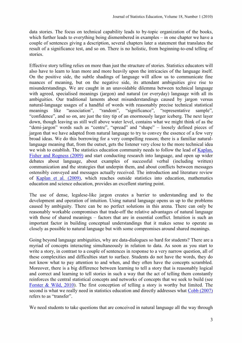
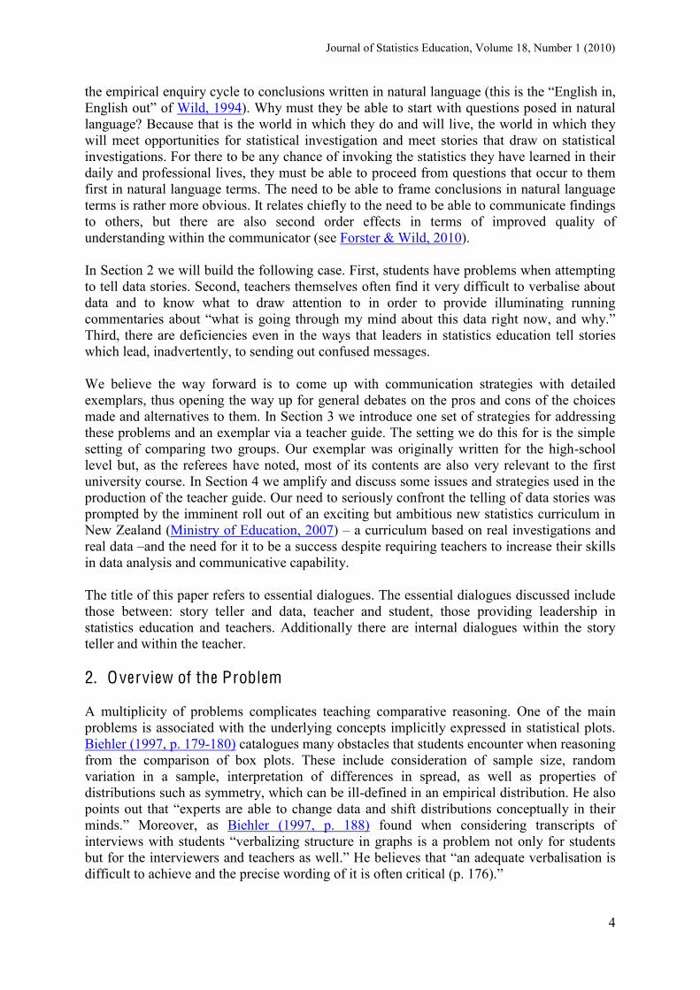
Pfannkuch and Horring (2005, p. 212) note that the teacher in their study avoided drawing conclusions and verbalizing her reasoning when comparing box plots. They conjecture that such a situation arose because textbooks and teaching compare or describe features of distributions and do not draw a conclusion since formal statistical inference is not introduced in New Zealand until the final year of school. To test this conjecture we searched through some introductory statistics textbooks (e.g., Wild & Seber, 2000; Moore & McCabe, 2003; de Veaux & Velleman, 2004; Agresti & Franklin, 2007; Moore, 2007; Utts & Heckard, 2007; Peck, Olsen, & Devore, 2008). We noted that all the books have a similar structure. The beginning chapters are devoted to constructing and reading plots descriptively, while the end chapters are focused on the procedures and technical aspects of conducting formal statistical inference. Not one of the books clearly demonstrated reasoning comparatively all of the way from looking at the plots, unlocking the story and the underlying concepts, and synthesising the whole data story through a transparent reasoning process. Rather, the focus is on the procedures to carry out and possible worries such as outliers, using the mean, and so forth. Pfannkuch and Horring (2005) conclude that articulating the messages contained in plots and justifying inferences either verbally or in writing are difficult problems to resolve for younger students but we believe that the problem should be tackled, discussed, debated and not be swept aside. Consider the following excerpt from the GAISE K-12 Report (2007, p. 47) describing the comparison of two box plots (Fig. 1). There is no investigative question posed, nor any conclusion drawn: just a commentary on the plots.

Figure 1. Sodium content of hot dogs. “The median sodium content for poultry hot dogs is 430 mg, almost 50mg more than the median sodium content for beef hot dogs. The medians indicate that a typical value for the sodium content of poultry hot dogs is greater than a typical value for beef hot dogs. The range for the beef hot dogs is 392 mg, versus 231 mg for the poultry hot dogs. The ranges indicate that, overall, there is more spread (variation) in the sodium content of beef hot dogs than poultry hot dogs.”

Poultry Beef

250 300 350 400 450 500 550 600 650 Sodium (mg)


6

We note a mix of descriptive statements about the sample distributions and inferential statements regarding the population distributions. This commentary seems to typify a tendency of statisticians to repeatedly switch between describing what they see in the samples and inferring what may be occurring in the underlying populations. A similar drift between descriptive and inferential thinking occurs in Utts and Heckard (2007, p. 469), de Veaux and Velleman (2004 , p. 459), Wild and Seber (2000, p. 429), and Moore (2007, p. 154, p. 158) when they attempt to introduce more of a story about the data. (This issue does not arise in many textbooks simply because of the way the chapters are partitioned into descriptive and inferential statistics procedures.) While statisticians accomplish such shuttling between thinking modes with unconscious ease, novices, including teachers, often do not recognise these two distinct ways of thinking, and when and why to engage in them. For example, Pfannkuch (2006, 2007) notes that, where the teacher was deliberately articulating her comparative reasoning, the teacher did not make the distinction between samples and populations with some of her statements being made about the sample, and some about the population from the sample. We have since found this problem is quite widespread. Pratt, Johnston-Wilder, Ainley and Mason (2008) also report teachers and students are confused about whether they are reasoning about the data as if it were the whole population or about a population from which the data are a sample. Other concepts emerge in the GAISE K-12 Report (2007, p. 48) in statements such as: “Considering the degree of variation in the data and the amount of overlap in the box plots, a difference of 50 mg between the medians is not really that large.”

Does this statement presuppose some fundamental experience of sampling variability and the sample size effect (sample sizes are 20 and 17) to be able to judge that the difference in centres is “not really that large” relative to the variability? Pfannkuch (2006) notes that students often misunderstand the term overlap, and that the teacher in her study used her “eye” and “feeling” to make a similar statements and judgments. Even though this teacher talked about sampling variability hypothetically, an analysis of students’ assessment responses suggested that her discourse was insufficient for student understanding of such statements (Pfannkuch, 2007). Or is the statement by the GAISE K-12 Report more about a “practical difference” in sodium content and made without consideration of sampling variability? Watson (2008) notes in her research that students seemed to be making judgments on perceived practical differences, which is similar to Makar and Confrey’s (2004) findings in their research on secondary teachers. We therefore question how the rich conceptual repertoire needed for interpreting statistical plots is built up in students’ understandings and experiences over the school years. As Chance, delMas, and Garfield (2004) and Makar and Confrey (2004) report, tertiary (university) students and teachers’ statistical inferential reasoning will continue to be limited unless ways of addressing verbalization and the building of a conceptual schema are developed in statistics teaching. The problem is particularly difficult as there are many concepts to attend to and simply addressing one concept is insufficient. For example, Pfannkuch (2008) experimented with developing 14 year-old students’ concepts of sampling variability using two web applications. The teacher and students knew about sampling variability and the links between sample and population but the problem of judging whether condition A tends to have bigger values than condition B still remained as the students and teacher continued to draw conclusions based on the difference between the medians without considering sampling variability. That is, they had no other criteria on which to base their decisions or ways of verbalizing what they had experienced.


7

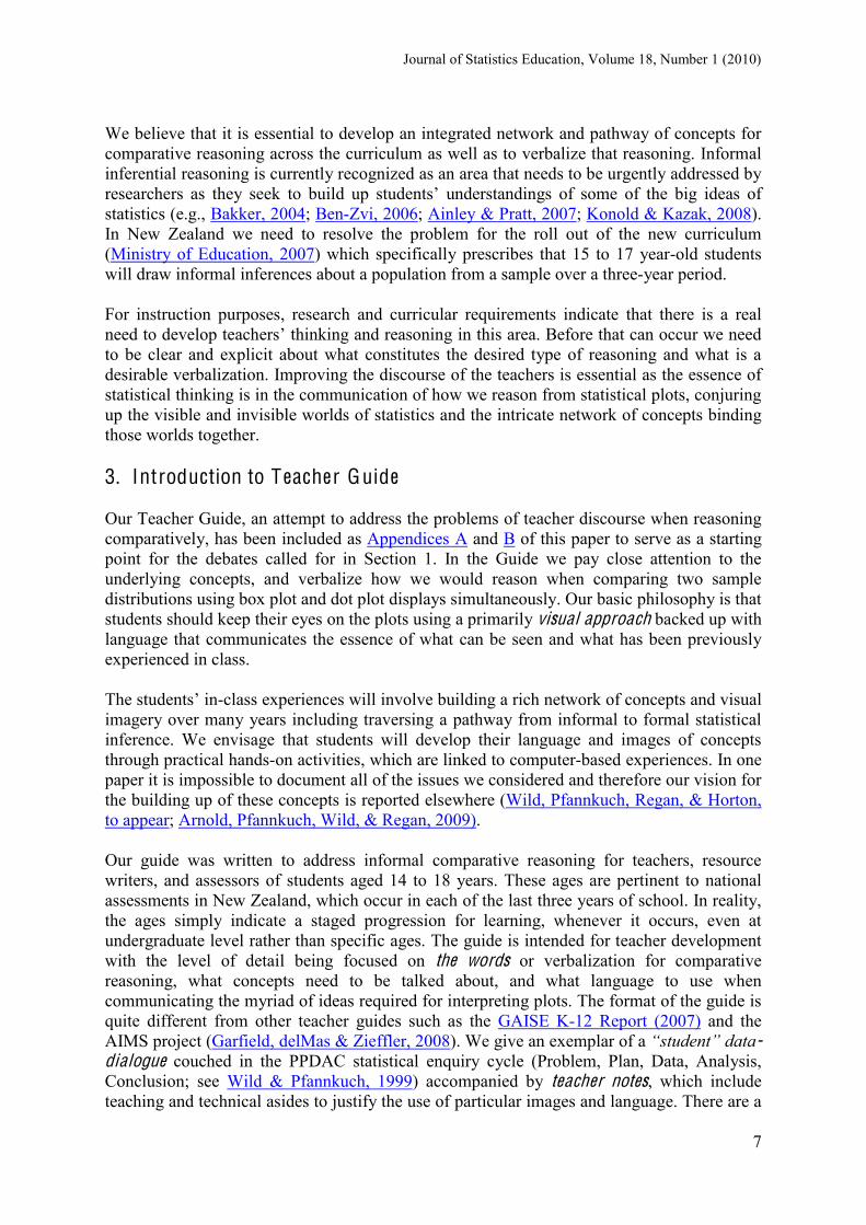
We believe that it is essential to develop an integrated network and pathway of concepts for comparative reasoning across the curriculum as well as to verbalize that reasoning. Informal inferential reasoning is currently recognized as an area that needs to be urgently addressed by researchers as they seek to build up students’ understandings of some of the big ideas of statistics (e.g., Bakker, 2004; Ben-Zvi, 2006; Ainley & Pratt, 2007; Konold & Kazak, 2008). In New Zealand we need to resolve the problem for the roll out of the new curriculum (Ministry of Education, 2007) which specifically prescribes that 15 to 17 year-old students will draw informal inferences about a population from a sample over a three-year period. For instruction purposes, research and curricular requirements indicate that there is a real need to develop teachers’ thinking and reasoning in this area. Before that can occur we need to be clear and explicit about what constitutes the desired type of reasoning and what is a desirable verbalization. Improving the discourse of the teachers is essential as the essence of statistical thinking is in the communication of how we reason from statistical plots, conjuring up the visible and invisible worlds of statistics and the intricate network of concepts binding those worlds together. 3. Introduction to Teacher Guide Our Teacher Guide, an attempt to address the problems of teacher discourse when reasoning comparatively, has been included as Appendices A and B of this paper to serve as a starting point for the debates called for in Section 1. In the Guide we pay close attention to the underlying concepts, and verbalize how we would reason when comparing two sample distributions using box plot and dot plot displays simultaneously. Our basic philosophy is that students should keep their eyes on the plots using a primarily visual approach backed up with language that communicates the essence of what can be seen and what has been previously experienced in class. The students’ in-class experiences will involve building a rich network of concepts and visual imagery over many years including traversing a pathway from informal to formal statistical inference. We envisage that students will develop their language and images of concepts through practical hands-on activities, which are linked to computer-based experiences. In one paper it is impossible to document all of the issues we considered and therefore our vision for the building up of these concepts is reported elsewhere (Wild, Pfannkuch, Regan, & Horton, to appear; Arnold, Pfannkuch, Wild, & Regan, 2009). Our guide was written to address informal comparative reasoning for teachers, resource writers, and assessors of students aged 14 to 18 years. These ages are pertinent to national assessments in New Zealand, which occur in each of the last three years of school. In reality, the ages simply indicate a staged progression for learning, whenever it occurs, even at undergraduate level rather than specific ages. The guide is intended for teacher development with the level of detail being focused on the words or verbalization for comparative reasoning, what concepts need to be talked about, and what language to use when communicating the myriad of ideas required for interpreting plots. The format of the guide is quite different from other teacher guides such as the GAISE K-12 Report (2007) and the AIMS project (Garfield, delMas & Zieffler, 2008). We give an exemplar of a “student” data-dialogue couched in the PPDAC statistical enquiry cycle (Problem, Plan, Data, Analysis, Conclusion; see Wild & Pfannkuch, 1999) accompanied by teacher notes, which include teaching and technical asides to justify the use of particular images and language. There are a


8

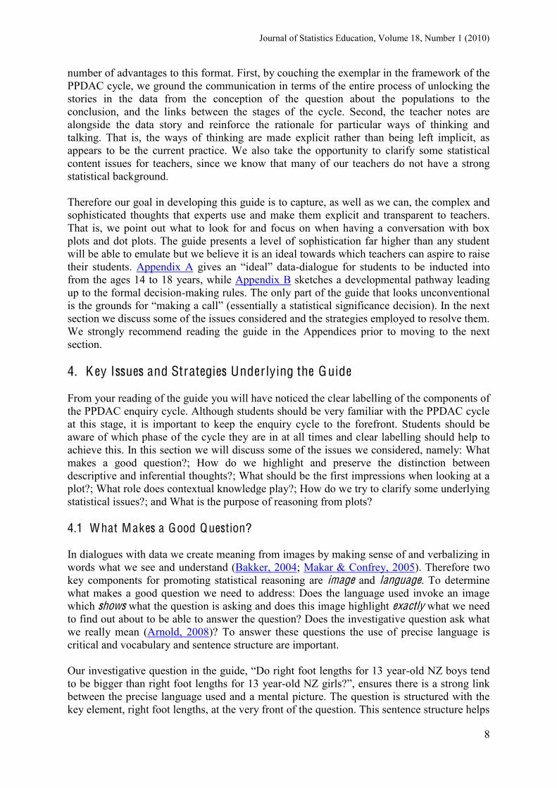
number of advantages to this format. First, by couching the exemplar in the framework of the PPDAC cycle, we ground the communication in terms of the entire process of unlocking the stories in the data from the conception of the question about the populations to the conclusion, and the links between the stages of the cycle. Second, the teacher notes are alongside the data story and reinforce the rationale for particular ways of thinking and talking. That is, the ways of thinking are made explicit rather than being left implicit, as appears to be the current practice. We also take the opportunity to clarify some statistical content issues for teachers, since we know that many of our teachers do not have a strong statistical background. Therefore our goal in developing this guide is to capture, as well as we can, the complex and sophisticated thoughts that experts use and make them explicit and transparent to teachers. That is, we point out what to look for and focus on when having a conversation with box plots and dot plots. The guide presents a level of sophistication far higher than any student will be able to emulate but we believe it is an ideal towards which teachers can aspire to raise their students. Appendix A gives an “ideal” data-dialogue for students to be inducted into from the ages 14 to 18 years, while Appendix B sketches a developmental pathway leading up to the formal decision-making rules. The only part of the guide that looks unconventional is the grounds for “making a call” (essentially a statistical significance decision). In the next section we discuss some of the issues considered and the strategies employed to resolve them. We strongly recommend reading the guide in the Appendices prior to moving to the next section. 4. K ey Issues and Strategies Under lying the Guide From your reading of the guide you will have noticed the clear labelling of the components of the PPDAC enquiry cycle. Although students should be very familiar with the PPDAC cycle at this stage, it is important to keep the enquiry cycle to the forefront. Students should be aware of which phase of the cycle they are in at all times and clear labelling should help to achieve this. In this section we will discuss some of the issues we considered, namely: What makes a good question?; How do we highlight and preserve the distinction between descriptive and inferential thoughts?; What should be the first impressions when looking at a plot?; What role does contextual knowledge play?; How do we try to clarify some underlying statistical issues?; and What is the purpose of reasoning from plots? 4.1 What Makes a Good Question? In dialogues with data we create meaning from images by making sense of and verbalizing in words what we see and understand (Bakker, 2004; Makar & Confrey, 2005). Therefore two key components for promoting statistical reasoning are image and language. To determine what makes a good question we need to address: Does the language used invoke an image which shows what the question is asking and does this image highlight exactly what we need to find out about to be able to answer the question? Does the investigative question ask what we really mean (Arnold, 2008)? To answer these questions the use of precise language is critical and vocabulary and sentence structure are important. Our investigative question in the guide, “Do right foot lengths for 13 year-old NZ boys tend to be bigger than right foot lengths for 13 year-old NZ girls?”, ensures there is a strong link between the precise language used and a mental picture. The question is structured with the key element, right foot lengths, at the very front of the question. This sentence structure helps


9

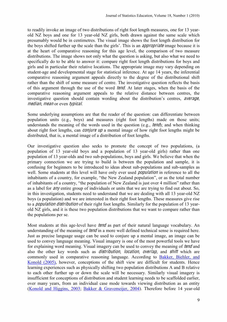
to readily invoke an image of two distributions of right foot length measures, one for 13 year-old NZ boys and one for 13 year-old NZ girls, both drawn against the same scale which presumably would be in centimetres. The visual image shows the foot length distribution for the boys shifted further up the scale than the girls’. This is an appropriate image because it is at the heart of comparative reasoning for this age level, the comparison of two measure distributions. The image shows not only what the question is asking, but also what we need to specifically do to be able to answer it: compare right foot length distributions for boys and girls and in particular their relative locations. The appropriate image may vary depending on student-age and developmental stage for statistical inference. At age 14 years, the inferential comparative reasoning argument appeals directly to the degree of the distributional shift rather than the shift of some measure of centre. The investigative question reflects the basis of this argument through the use of the word tend. At later stages, when the basis of the comparative reasoning argument appeals to the relative distance between centres, the investigative question should contain wording about the distribution’s centres, average, median, mean or even typical. Some underlying assumptions are that the reader of the question: can differentiate between population units (e.g., boys) and measures (right foot lengths) made on those units; understands the meaning of the words used in the question (e.g., tend); and when thinking about right foot lengths, can conjure up a mental image of how right foot lengths might be distributed, that is, a mental image of a distribution of foot lengths. Our investigative question also seeks to promote the concept of two populations, (a population of 13 year-old boys and a population of 13 year-old girls) rather than one population of 13 year-olds and two sub-populations, boys and girls. We believe that when the primary connection we are trying to build is between the population and sample, it is confusing for beginners to be introduced to ideas about sub-populations and sub-samples as well. Some students at this level will have only ever used population in reference to all the inhabitants of a country, for example, “the New Zealand population”, or as the total number of inhabitants of a country, “the population of New Zealand is just over 4 million” rather than as a label for any entire group of individuals or units that we are trying to find out about. So, in this investigation, students need to understand that we are dealing with all 13 year-old NZ boys (a population) and we are interested in their right foot lengths. These measures give rise to a population distribution of their right foot lengths. Similarly for the population of 13 year-old NZ girls, and it is these two population distributions that we want to compare rather than the populations per se. Most students at this age-level have tend as part of their natural language vocabulary. An understanding of the meaning of tend in a more well defined technical sense is required here. Just as precise language usage can be used to conjure up a mental image, an image can be used to convey language meaning. Visual imagery is one of the most powerful tools we have for explaining word meaning. Visual imagery can be used to convey the meaning of tend and also the other key words such as distribution, location, overlap, and shift which are commonly used in comparative reasoning language. According to Bakker, Biehler, and Konold (2005), however, conceptions of the shift view are difficult for students. Hence learning experiences such as physically shifting two population distributions A and B relative to each other further up or down the scale will be necessary. Similarly visual imagery is insufficient for conceptions of distribution and student learning needs to be scaffolded earlier, over many years, from an individual case mode towards viewing distribution as an entity (Konold and Higgins, 2003; Bakker & Gravemeijer, 2004). Therefore before 14 year-old


10

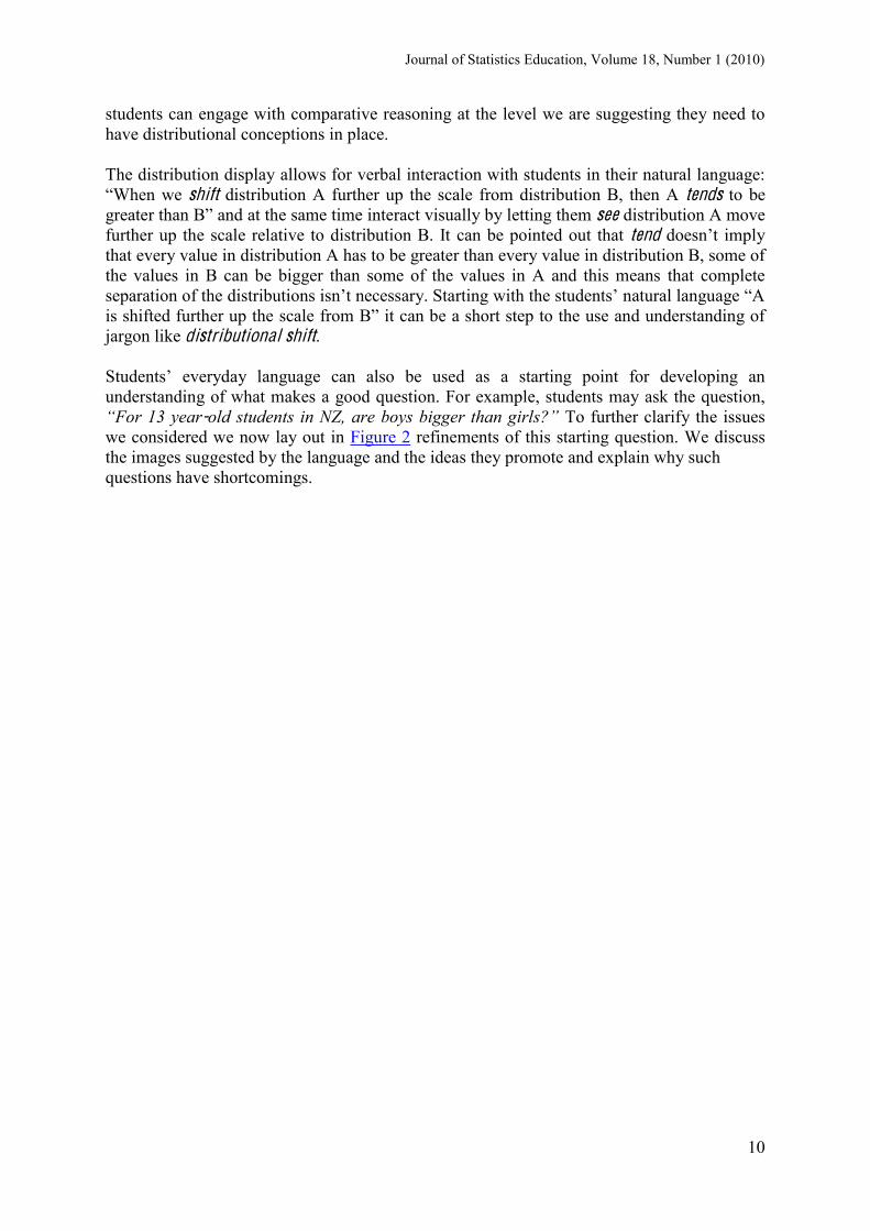
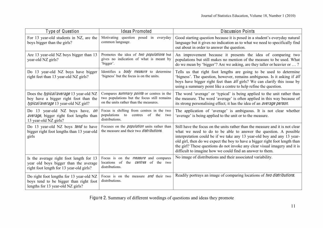
students can engage with comparative reasoning at the level we are suggesting they need to have distributional conceptions in place. The distribution display allows for verbal interaction with students in their natural language: “When we shift distribution A further up the scale from distribution B, then A tends to be greater than B” and at the same time interact visually by letting them see distribution A move further up the scale relative to distribution B. It can be pointed out that tend doesn’t imply that every value in distribution A has to be greater than every value in distribution B, some of the values in B can be bigger than some of the values in A and this means that complete separation of the distributions isn’t necessary. Starting with the students’ natural language “A is shifted further up the scale from B” it can be a short step to the use and understanding of jargon like distributional shift. Students’ everyday language can also be used as a starting point for developing an understanding of what makes a good question. For example, students may ask the question, “For 13 year-old students in NZ, are boys bigger than girls?” To further clarify the issues we considered we now lay out in Figure 2 refinements of this starting question. We discuss the images suggested by the language and the ideas they promote and explain why such questions have shortcomings.


11

Type of Question Ideas Promoted Discussion Points

For 13 year-old students in NZ, are the boys bigger than the girls?

Motivating question posed in everyday common language.

Good starting question because it is posed in a student’s everyday natural language but it gives no indication as to what we need to specifically find out about in order to answer the question.

Are 13 year-old NZ boys bigger than 13 year-old NZ girls?

Promotes the idea of two populations but gives no indication of what is meant by ‘bigger’.

An improvement because it presents the idea of comparing two populations but still makes no mention of the measure to be used. What do we mean by ‘bigger’? Are we asking, are they taller or heavier or … ?

Do 13 year-old NZ boys have bigger right feet than 13 year-old NZ girls?

Identifies a body measure to determine ‘bigness’ but the focus is on the units.

Tells us that right foot lengths are going to be used to determine ‘bigness’. The question, however, remains ambiguous. Is it asking if all boys have bigger right feet than all girls? We can clarify this issue by using a summary point like a centre to help refine the question.

Does the typical/average 13 year-old NZ boy have a bigger right foot than the typical/average 13 year-old NZ girl?

Compares summary points or centres in the two populations but the focus still remains on the units rather than the measures.

The word ‘average’ or ‘typical’ is being applied to the unit rather than the measure. The word ‘average’ is often applied in this way because of its strong personalising effect; it has the idea of an average person.

Do 13 year-old NZ boys have, on average, bigger right foot lengths than 13 year-old NZ girls?

Focus is shifting from centres in the two populations to centres of the two distributions.

The application of ‘average’ is ambiguous. It is not clear whether ‘average’ is being applied to the unit or to the measure.

Do 13 year-old NZ boys tend to have bigger right foot lengths than 13 year-old girls

Focuses on the population units rather than the measure and their two distributions.

Still have the focus on the units rather than the measure and it is not clear what we need to do to be able to answer the question. A possible interpretation could be if we take any 13 year-old boy and any 13 year-old girl, then do we expect the boy to have a bigger right foot length than the girl? These questions do not invoke any clear visual imagery and it is difficult to imagine how we could find an answer to them.

Is the average right foot length for 13 year old boys bigger than the average right foot length for 13 year-old girls?

Focus is on the measure and compares locations of the centres of the two distributions.

No image of distributions and their associated variability.

Do right foot lengths for 13 year-old NZ boys tend to be bigger than right foot lengths for 13 year-old NZ girls?

Focus is on the measure and their two distributions.

Readily portrays an image of comparing locations of two distributions.

F igure 2. Summary of different wordings of questions and ideas they promote


12

4.2 How do we H ighlight and Preserve the Distinction between Descr iptive and Inferential Thoughts?

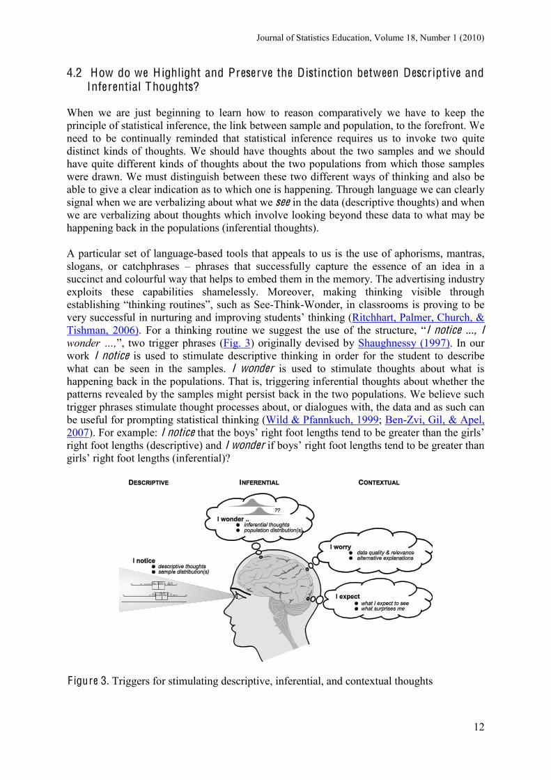
When we are just beginning to learn how to reason comparatively we have to keep the principle of statistical inference, the link between sample and population, to the forefront. We need to be continually reminded that statistical inference requires us to invoke two quite distinct kinds of thoughts. We should have thoughts about the two samples and we should have quite different kinds of thoughts about the two populations from which those samples were drawn. We must distinguish between these two different ways of thinking and also be able to give a clear indication as to which one is happening. Through language we can clearly signal when we are verbalizing about what we see in the data (descriptive thoughts) and when we are verbalizing about thoughts which involve looking beyond these data to what may be happening back in the populations (inferential thoughts). A particular set of language-based tools that appeals to us is the use of aphorisms, mantras, slogans, or catchphrases – phrases that successfully capture the essence of an idea in a succinct and colourful way that helps to embed them in the memory. The advertising industry exploits these capabilities shamelessly. Moreover, making thinking visible through establishing “thinking routines”, such as See-Think-Wonder, in classrooms is proving to be very successful in nurturing and improving students’ thinking (Ritchhart, Palmer, Church, & Tishman, 2006). For a thinking routine we suggest the use of the structure, “I notice ..., I wonder …,”, two trigger phrases (Fig. 3) originally devised by Shaughnessy (1997). In our work I notice is used to stimulate descriptive thinking in order for the student to describe what can be seen in the samples. I wonder is used to stimulate thoughts about what is happening back in the populations. That is, triggering inferential thoughts about whether the patterns revealed by the samples might persist back in the two populations. We believe such trigger phrases stimulate thought processes about, or dialogues with, the data and as such can be useful for prompting statistical thinking (Wild & Pfannkuch, 1999; Ben-Zvi, Gil, & Apel, 2007). For example: I notice that the boys’ right foot lengths tend to be greater than the girls’ right foot lengths (descriptive) and I wonder if boys’ right foot lengths tend to be greater than girls’ right foot lengths (inferential)?

F igure 3. Triggers for stimulating descriptive, inferential, and contextual thoughts


13

I notice stresses that we are making a statement about what we see regarding the foot lengths of the boys and the girls in our samples, that is, for these particular boys and these particular girls. In the language we signal that we are describing patterns for these particular boys and girls with the use of the definite article the (or even these) which is absent from the I wonder statement. The distinction between descriptive and inferential thoughts is so critical that we recommend that when we verbalise inferential thoughts in comparative reasoning we should, in the beginning, always add the phrase “back in the two populations”. For example “I wonder if boys’ foot lengths tend to be bigger than girls’ back in the two populations”. It is an opportunity to repetitively stress that inferential thoughts involve a conjecture about two population distributions and not a description of comparison of the two sample distributions. Repetitive use of the phrase should further cement in the concepts and imagery involved when comparing two population distributions. The language may appear awkward but that awkwardness should attract students’ attention and help them to remember the phrase which in turn will repeatedly trigger these ideas, concepts, and imagery. This structure will not only serve as a trigger as to when it is appropriate to have these kinds of thoughts but the I wonder prefix will also protect us from using language which, strictly speaking, describes what is happening back in the population rather than making conjectures or suggestions. For example: “Boys’ foot lengths tend to be greater than girls’ foot lengths” leaves us in doubt as to whether this is just the use of loose language in an attempt to make a descriptive statement comparing the sample distributions or whether in fact it is intended to be a conclusive statement about the population distributions based on “what you see in the data is what is happening in the populations.” That is, having no regard for sampling variability. The ‘I wonder’ statement begs a response and therefore leads on naturally to some form of testing the conjecture. An alternative is to use suggestive-type language. For example, “The sample distributions suggest that boys’ foot lengths tend to be bigger than girls”. Suggestive language can be seen to be more terminating in the sense that it does not seem to invite a response and therefore may be more appropriate in the very first introductions to informal statistical inference. The suggestive nature of the language serves as an acknowledgement of uncertainty due to sampling variability and therefore acknowledges that both descriptive and inferential thinking have occurred. Other suggestive-type phrases are: “It appears that boys’ foot lengths tend to be bigger than girls ”, “It seems that...”, “It looks as if...” or even “The sample distributions indicate that boys’ foot lengths tend to be bigger than girls”. We would prefer not to use “indicate” as it is a lot less suggestive than the other examples and is quite close in meaning to “show” which is confirmatory rather than suggestive. It would be necessary, however, to draw students’ attention to the use of suggestive language and how it is used to suggest what might be happening back in the populations based on what has been observed in the sample data and should not used when simply making descriptive statements about sample data. A disadvantage of using the I notice, I wonder structure is that, in reality, there is strong interplay between descriptive and inferential thoughts. There is a continual and rapid switching back and forth between these two kinds of thoughts. It is not the case, as the I notice, I wonder structure suggests that we have descriptive thoughts which are then followed by inferential thoughts. In fact, our descriptive thoughts are largely influenced by inferential thoughts and vice versa. For example, what actually gets recorded or commented on


14

descriptively are the remarkable features in the data, the “remarkableness” being largely determined from inferential thinking. I notice invites students to comment on every single feature including small gaps, hints of skewness and naming all of the statistical summaries, which is not statistical thinking. As Wild (2006, p. 20) points out statistical thinking occurs when “we move beyond name calling” and “relate features we can see and name in our data set, and believe will persist” in the population. However, we think the advantages of the structure as discussed in the preceding paragraphs far outweigh these disadvantages. 4.3 What Should be the F irst Impressions When Looking at a Plot? As well as keeping the sample and population ideas to the forefront we also wish to capture the main features – overlap, shift, and unusual features – of the sample plots before any other analysis is conducted. The reason for the attention to these main features is because overlap and shift notions are fundamental in making an inferential claim about whether one group tends to have higher values than the other. Unusual features, such as outliers, are often the first features noticed intuitively by students. We acknowledge this intuitive noticing at the first reading of the data and address it later under the individual reasoning element using the trigger I worry to turn attention to measurement issues, whether the data should be cleaned or not, or further investigated (Fig. 3). Attention to these three features reinforces that comparisons are made between groups and within each group, something that teachers are not good at elucidating (Pfannkuch, 2006). Once students notice the overlap, shift, and unusual features using an overall visual approach, they can then start a more detailed analysis or dialogue with the sample data. The analysis seeks to activate different ways of looking at the plots through splitting the desired reasoning into components. These components of reasoning are based on a model developed by Pfannkuch (2006, 2007), which Watson (2008) also adapted to assess students’ comparative reasoning. Such a structure can assist teachers to develop the many aspects of comparative reasoning. We envisage that students will build up these reasoning components over a number of years. Starting at ages 9 and 10 years in the new New Zealand curriculum (Ministry of Education, 2007), students will describe features of dot plots, and at ages 11 to 13 students will make descriptive statements about two samples through visually comparing dot plots. Therefore, the reasoning elements described in the Analysis section of this document (Overall visual comparisons; Shift and overlap; Summary; Spread; Shape, Individual, and Gaps/Clusters) should already be embedded into students’ thinking to some extent. By stressing all the reasoning components involved in comparison we wish to emphasize that point estimates and zeroing in on immediately making a call are insufficient and only a very small part of the underlying rich conceptual repertoire and data-dialogue. 4.4 What Role does Contextual K nowledge Play? Within the reasoning components, as well as the whole PPDAC cycle, contextual knowledge plays an important role in the data-dialogue (Wild & Pfannkuch, 1999). For example, consider the following excerpt from the GAISE K-12 Report (2007, p. 48) (see Fig. 1)

“The IQRs suggest that the spread within the middle half of the data for beef hot dogs is similar to the spread within the middle half of the data for poultry hot dogs. The boxplots also suggest that each distribution is somewhat skewed right.”

In order to believe whether these features do or do not persist back in the two populations we need to draw on our statistical knowledge about sampling variability and on our contextual knowledge to determine whether further investigation of the data is warranted. Recognizing


15

and thinking about why a sample distribution might depart from what is expected is a key aspect of reasoning from data. Our strategy for acknowledging that contextual knowledge is used for determining whether a pattern persists back in the population is to use the words I expect so (Fig. 3). We also realised that students may not have the contextual knowledge needed to allow them to have expectations about the nature of the population distribution so we suggested that students sketch plausible distribution shapes and the relative location of the populations when initially posing the investigative question. Other reasons for such an approach are that teachers can observe students’ prior conceptions and images such as whether they draw similar shaped distributions in the same location with one distribution having a higher mound than the other or draw similar shaped distributions with different locations. Furthermore, teachers report to us that they do not currently build up in students a sense of the shape of distributions they might expect for different measurement variables (see also Bakker & Gravemeijer, 2004). 4.5 How do we T ry to C larify Some Under lying Statistical Issues? The interquartile range is mentioned by the GAISE K-12 Report (2007, p. 47) as “another measure of spread that should be introduced at Level B” but no rationale for its introduction is given. A similar situation exists in teaching where students simply learn calculations for the five-number summaries but not how or why these summaries assist in reasoning comparatively. Since many teachers do not have strong background knowledge in statistics, our strategy is to clearly state why the IQR is a more robust measure of spread than the range in the teacher dialogue and to demote the use of range by using faint text in the student dialogue. We have used faint text in other parts of the guide as well, for example, as a signal that we noticed a hint of bimodality in the data but we should not read much into it. You will have noticed Teaching Tips in the commentary section of the guide. A number of these teaching tips have an accompanying Technical Note. We have used Technical Notes to attempt to explain the rationale behind the teaching tip. We also use technical notes to give some background statistical information on issues which we have identified as being problematic for some teachers. 4.6 What is the Purpose of Reasoning from Plots? The GAISE K-12 Report (2007) creates a pathway through the curriculum by focusing on different aspects of comparative reasoning through a pre-K-12 curriculum framework with Levels A, B, and C. At Level C they use re-sampling methods to enable students to make a claim. However, we believe that decision-making should be an earlier goal for students, otherwise reasoning from data seems to lack purpose and direction and thus results in a lowering of the interest-factor level for students. We have two main strategies to provide purpose to comparative reasoning. Our first strategy is to structure comparative reasoning around the statistical enquiry cycle. In this way we can highlight the purpose of the comparison by starting with an investigative question. Furthermore, we can stress that the question or problem is about the population (Arnold, 2008), as well as emphasize the thinking that is incurred before the analysis stage. After making a call, the conclusion stage, we acknowledge that statistical enquiry requires us to determine whether the findings make sense with what we know about the real situation from our contextual knowledge (Pfannkuch, 2006). Our strategy is to deal with sampling variability first, make the appropriate call, and then use contextual knowledge to think of


16

other factors or alternative explanations that might explain what has been seen (Fig. 3). Our second strategy for facilitating purposeful comparative reasoning is to concentrate on sampling variability by creating a pathway through the curriculum for 14 to 18 year-olds on ways to make a decision under uncertainty. The pathway begins inference simply and then moves to increasingly sophisticated tools and ideas. These developmental “decision-rules” (Appendix B), backed up by in depth experiences of sampling variability, will enable students to make a judgment on or make a call on which population tends to have bigger values. We deliberately use which is bigger rather than are they different or the same in an attempt to eliminate thinking under the null from beginning experiences of inference and no difference misconceptions (see Wild et al., to appear, Section 2.5). If we cannot make a call because we are unsure of the direction of the population patterns, we simply state we are not prepared to make a call on the basis of the information provided. Whereas use of the terms difference or same invites students to make the claim that two populations are the same. 5. Concluding Remarks In general, textbooks do not demonstrate reasoning comparatively from looking at the plots, unlocking the story, attending to the underlying concepts, and synthesising the whole data story through a transparent reasoning process. In the teacher guide we attempted to highlight the importance of looking at plots and to explicate the extent of the rich conceptual repertoire that needs to be prompted when unlocking stories in data. We uncovered some of the essential dialogues for facilitating the synthesizing of the whole data story which are currently implicit (e.g., GAISE K-12 Report, 2007) or not addressed because textbooks are partitioned into descriptive and inferential procedures. Technology is freeing teachers from the task of focusing their teaching on the construction of plots. Instead teachers can enhance and promote the true purpose of statistics: to learn more about real-world situations. This involves drawing inferences from sample data about a wider universe taking sampling variability into account and making a decision under uncertainty. Because comparative reasoning is so complex its development should take place in students over many years. In this transition, however, from teaching construction of plots to attending to conceptual reasoning from plots, the reasoning of teachers will also need to be developed. Without a guide on the essential data-dialogue that needs to be engaged in when reasoning comparatively, teachers will be cast adrift not knowing how rich the concepts are and how to adequately verbalize those concepts. The issues we have raised in the production of this guide and our strategies to deal with them are only a small part of the robust debates and discussions we have had. We hope that the guide will raise some issues and provoke detailed debates about desirable ways of reasoning comparatively and desirable verbalizations. Let the debates begin! Acknowledgements This work is supported by a grant from the Teaching and Learning Research Initiative (http://www.tlri.org.nz/). We thank the referees for their very helpful comments.

http://www.tlri.org.nz/


17

References Agresti, A., & Franklin, C. (2007). Statistics: The art and science of learning from data. Upper Saddle River, NJ: Pearson Prentice Hall. Arnold, P. (2008). What about the P in the PPDAC cycle? An initial look at posing questions for statistical investigation. In Proceedings of the 11th International Congress of Mathematics Education. Monterrey, Mexico, 6-13 July, 2008, http://tsg.icme11.org/tsg/show/15

Arnold, P., Pfannkuch, M., Wild, C.J., & Regan, M. (2009). Sampling variation for informal inference: F rom physical activities to computer animations. Unpublished paper.

Ainley, J., &. Pratt, D. (Eds.) (2007). Proceedings of the F ifth International Research Forum on Statistical Reasoning, Thinking and Literacy: Reasoning about Statistical Inference: Innovative Ways of Connecting Chance and Data. The University of Warwick, 11-17 November 2007.

Bakker, A. (2004). Reasoning about shape as a pattern in variability. Statistics Education Research Journal, 3(2), 64-83, http://www.stat.auckland.ac.nz/serj

Bakker, A., Biehler, R., & Konold, C. (2005). Should young students learn about boxplots? In G. Burrill & M. Camden (Eds.), Curricular development in statistics education: International Association for Statistical Education (IASE) Roundtable, Lund, Sweden 28 June-3 July 2004, (pp. 163-173). Voorburg, The Netherlands: International Statistical Institute. Online: http://www.stat.auckland.ac.nz/~iase/publications.php

Bakker, A., & Gravemeijer, K. (2004). Learning to reason about distribution. In D. Ben-Zvi & J. Garfield (Eds.), The challenge of developing statistical literacy, reasoning, and thinking (pp. 147−168). Dordrecht, The Netherlands: Kluwer Academic Publishers. Ben-Zvi, D. (2006). Scaffolding students’ informal inference and argumentation. In A. Rossman & B. Chance (Eds.), Proceedings of the Seventh International Conference on Teaching Statistics, Salvador, Brazil, July, 2006: Working cooperatively in statistics education. [CD-ROM]. Voorburg, The Netherlands: International Statistical Institute. Online: http://www.stat.auckland.ac.nz/~iase/publications.php

Ben-Zvi, D., Gil, E., & Apel, N. (2007). What is hidden beyond the data? Helping young students to reason and argue about some wider universe. In J. Ainley and D. Pratt (Eds.), Proceedings of the F ifth International Research Forum on Statistical Reasoning, Thinking and Literacy: Reasoning about Statistical Inference: Innovative Ways of Connecting Chance and Data. The University of Warwick, (1-26), 11-17 November 2007. Biehler, R. (1997). Students’ difficulties in practicing computer-supported data analysis:

http://www.stat.auckland.ac.nz/~iase/publications.php

http://tsg.icme11.org/tsg/show/15

http://www.stat.auckland.ac.nz/serj



18

Some hypothetical generalizations from results of two exploratory studies. In J. Garfield & G. Burrill (Eds.), Research on the role of technology in teaching and learning statistics (pp. 169-190). Voorburg, The Netherlands: International Statistical Institute. Online: http://www.stat.auckland.ac.nz/~iase/publications.php Chance, B., delMas, R., & Garfield, J. (2004). Reasoning about sampling distributions. In D. Ben-Zvi and J. Garfield (Eds.), The challenge of developing statistical literacy, reasoning and thinking (pp. 295-324). Dordrecht, The Netherlands: Kluwer Academic Publishers.

Cobb, G. (2007). One possible frame for thinking about experiential learning. International Statistical Review, 75(3), 336-347.

De Veaux, R., & Velleman, P. (2004). Intro Stats. New York: Pearson Addison Wesley.

Forster, M., & Wild, C.J. (In press - 2010). Writing about findings: Integrating teaching and assessment. In P. Bidgood, N. Hunt, F. Jolliffe (Eds.), Variety in Statistics Assessment. New York: Wiley-Blackwell.

Francis, (2005). An approach to report writing in statistics courses. In B. Phillips & K.L. Weldon (Eds.). Proceedings of the IASE Satellite Conference on Statistics Education and the Communication of Statistics. Voorburg, The Netherlands : International Statistical Institute. Online: http://www.stat.auckland.ac.nz/~iase/publications.php?show=14

GAISE K-12 Report (2007). Guidelines for assessment and instruction in statistics education (GAISE) report: a pre-k-12 curriculum framework. Alexandria, VA: American Statistical Association. Online: http://www.amstat.org/education/gaise

Garfield, J., delMas, R., & Zieffler, A. (2008). AIMS Project Adapting and Implementing Innovative Material in Statistics: Aims topics. Online: http://www.tc.umn.edu/~aims/aimstopics.htm

Holmes, P. (1997). Assessing project work by external examiners. In I. Gal and J. Garfield (Eds.), The assessment challenge in statistics education (pp. 153-164). Amsterdam: IOS Press.

Kaplan, J.J., Fisher, D. & Rogness, N. (2009). Lexical Ambiguity in Statistics: What do students know about the words: association, average, confidence, random and spread? Journal of Statistics Education, 17(3), http://www.amstat.org/publications/jse/contents_2009.html

Konold, C., & Higgins, T. (2003). Reasoning about data. In J. Kilpatrick, W. G. Martin, & D. Schifter, (Eds.), A research companion to Principles and Standards for School Mathematics (pp. 193-214). Reston, VA: National Council of Teachers of Mathematics.

Konold, C., & Kazak, S. (2008). Reconnecting data and chance. Technology Innovations in Statistics Education, 2(1). Online: http://repositories.cdlib.org/uclastat/cts/tise/vol2/iss1/art1/

http://repositories.cdlib.org/uclastat/cts/tise/vol2/iss1/art1/


http://www.stat.auckland.ac.nz/~iase/publications.php?show=14

http://www.amstat.org/education/gaise

http://www.tc.umn.edu/~aims/aimstopics.htm

http://www.amstat.org/publications/jse/contents_2009.html


19

MacGillivray, H. (2005). Helping Students Find Their Statistical Voices. In B. Phillips & K.L. Weldon (Eds.). Proceedings of the IASE Satellite Conference on Statistics Education and the Communication of Statistics. Voorburg, The Netherlands: International Statistical Institute. Online: http://www.stat.auckland.ac.nz/~iase/publications.php?show=14

Makar, K., & Confrey, A. (2004). Secondary teachers’ statistical reasoning in comparing two groups. In D. Ben-Zvi & J. Garfield (Eds.), The challenge of developing statistical literacy, reasoning, and thinking (pp. 353−373). Dordrecht, The Netherlands: Kluwer Academic Publishers.

Makar, K., & Confrey, J. (2005). “Variation-Talk”: Articulating meaning in statistics. Statistics Education Research Journal, 4(1), 27-54, http://www.stat.auckland.ac.nz/serj

Ministry of Education (2007). The New Zealand Curriculum. Wellington, New Zealand: Learning Media Limited.

Moore, D. (1998). Statistics among the liberal arts. Journal of the American Statistical Association, 93(444), 1253-1259.

Moore, D. (2007). The basic practice of statistics (4th edition). New York: W. H. Freeman and Company.

Moore, D., & McCabe, G. (2003). Introduction to the practice of statistics (4th edition). New York: W. H. Freeman and Company.

Peck, R., Olsen, C., & Devore, J. (2008). Introduction to statistics and data analysis (3rd edition). Belmont, CA: Thomson Brooks/Cole.

Pfannkuch, M. (2005). Probability and statistical inference: How can teachers enable learners to make the connection? In G. Jones (Ed.), Exploring probability in school: Challenges for teaching and learning, (pp. 267-294). New York: Springer.

Pfannkuch, M. (2006). Comparing box plot distributions: A teacher’s reasoning. Statistics Education Research Journal, 5(2), 27-45, http://www.stat.auckland.ac.nz/serj

Pfannkuch, M. (2007). Year 11 students’ informal inferential reasoning: A case study about the interpretation of box plots. International Electronic Journal of Mathematics Education, 2(3), 149-167, http://www.iejme.com/

Pfannkuch, M. (2008). Building sampling concepts for statistical inference: A case study. In ICME-11 Proceedings, Monterrey, Mexico, July 2008, http://tsg.icme11.org/tsg/show/15.

Pfannkuch, M., & Horring, J. (2005). Developing statistical thinking in a secondary school: A collaborative curriculum development. In G. Burrill & M. Camden (Eds.), Curricular development in statistics education: International Association for Statistical Education

http://tsg.icme11.org/tsg/show/15

http://www.stat.auckland.ac.nz/~iase/publications.php?show=14



http://www.iejme.com/


20

(IASE) Roundtable, Lund, Sweden 28 June-3 July 2004, (pp. 204-218). Voorburg, The Netherlands: International Statistical Institute.

Pratt, D., Johnston-Wilder, P., Ainley, J., & Mason, J. (2008). Local and global thinking in statistical inference. Statistics Education Research Journal, 7(2), 107-129, http://www.stat.auckland.ac.nz/serj

Ritchhart, R., Palmer, P., Church, M., & Tishman, S. (2006). Thinking routines: Establishing patterns of thinking in the classroom. Paper presented at The American Educational Research Association (AERA) Annual Conference, Chicago, April, 2006.

Rosling, H. (2006). Debunking myths about the ‘Third world’. TED2006 conference. Online: www.gapminder.org/videos/ted-talks/hans-rosling-ted-2006-debunking-myths-about-the-third-world/ Rosling, H. (2007). The seemingly impossible is possible. TED2007 conference. Online: www.gapminder.org/videos/ted-talks/hans-rosling-ted-talk-2007-seemingly-impossible-is-possible/

Shaughnessy, J. M. (1997). Missed opportunities in research on the teaching and learning of data and chance. In F. Biddulph & K. Carr (Eds.), Proceedings of the 20th Annual Conference of the Mathematics Education Research Group of Australasia, Rotorua, New Zealand, July, 2007: People in mathematics education (Vol.1, pp. 6-22). Sydney: MERGA.

Starkings, S. (1997). Assessing student projects. In I. Gal and J. Garfield (Eds.), The assessment challenge in statistics education (pp. 139-152). Amsterdam: IOS Press.

Utts, J., & Heckard, R. (2007). Mind on statistics (3rd edition). Belmont, CA: Thomson Brooks/Cole.

Watson, J. (2008). Exploring beginning inference with novice grade 7 students. Statistics Education Research Journal, 7(2), 59-82, http://www.stat.auckland.ac.nz/serj

Wild, C.J. (1994). Embracing the “wider view” of statistics. The American Statistician, 48(2), 163-171

Wild, C.J. (2006). The concept of distribution. Statistics Education Research Journal, 5(2), 10-26, http://www.stat.auckland.ac.nz/serj

Wild, C.J. (2007). Virtual environments and the acceleration of experiential learning. International Statistical Review, 75(3), 322-335.

Wild, C.J. & Pfannkuch, M. (1999). Statistical Thinking in Empirical Enquiry (with discussion). International Statistical Review, 67(3), 223-265.



http://www.gapminder.org/videos/ted-talks/hans-rosling-ted-2006-debunking-myths-about-the-third-world/

http://www.gapminder.org/videos/ted-talks/hans-rosling-ted-2006-debunking-myths-about-the-third-world/

http://www.gapminder.org/videos/ted-talks/hans-rosling-ted-talk-2007-seemingly-impossible-is-possible/

http://www.gapminder.org/videos/ted-talks/hans-rosling-ted-talk-2007-seemingly-impossible-is-possible/



21

Wild, C.J., Pfannkuch, M., Regan, M., & Horton, N.J. (to appear – accepted, not yet in press). Towards more accessible conceptions of statistical inference. Journal of the Royal Statistical Society Series A.

Wild, C.J., & Seber, G.A.F. (2000). Chance encounters: A first course in data analysis and inference. New York: John Wiley and Sons.


22

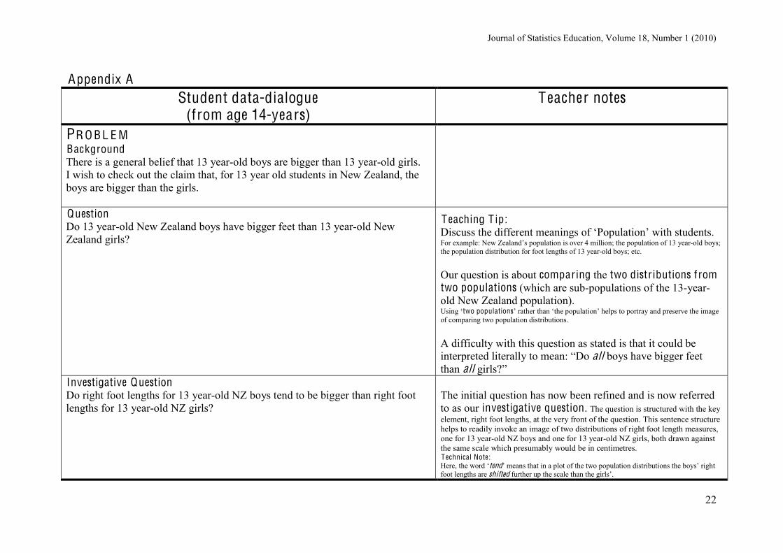
Appendix A Student data-dialogue

(from age 14-years) T eacher notes

PR O B L E M Background There is a general belief that 13 year-old boys are bigger than 13 year-old girls. I wish to check out the claim that, for 13 year old students in New Zealand, the boys are bigger than the girls.

Question Do 13 year-old New Zealand boys have bigger feet than 13 year-old New Zealand girls?

T eaching T ip: Discuss the different meanings of ‘Population’ with students. For example: New Zealand’s population is over 4 million; the population of 13 year-old boys; the population distribution for foot lengths of 13 year-old boys; etc. Our question is about comparing the two distr ibutions from two populations (which are sub-populations of the 13-year-old New Zealand population). Using ‘two populations’ rather than ‘the population’ helps to portray and preserve the image of comparing two population distributions. A difficulty with this question as stated is that it could be interpreted literally to mean: “Do all boys have bigger feet than all girls?”

Investigative Question Do right foot lengths for 13 year-old NZ boys tend to be bigger than right foot lengths for 13 year-old NZ girls?

The initial question has now been refined and is now referred to as our investigative question. The question is structured with the key element, right foot lengths, at the very front of the question. This sentence structure helps to readily invoke an image of two distributions of right foot length measures, one for 13 year-old NZ boys and one for 13 year-old NZ girls, both drawn against the same scale which presumably would be in centimetres. T echnical Note: Here, the word ‘tend’ means that in a plot of the two population distributions the boys’ right foot lengths are shifted further up the scale than the girls’.


23

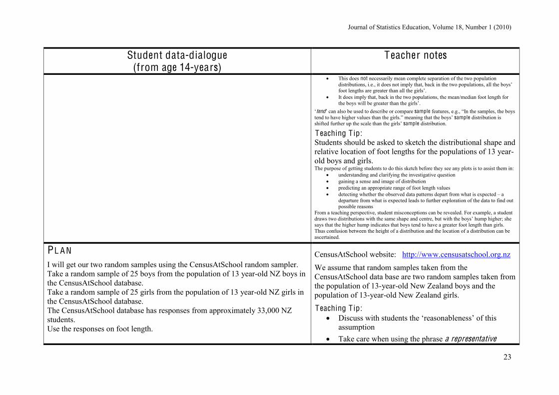
Student data-dialogue (from age 14-years)

T eacher notes

This does not necessarily mean complete separation of the two population distributions, i.e., it does not imply that, back in the two populations, all the boys’ foot lengths are greater than all the girls’.

It does imply that, back in the two populations, the mean/median foot length for the boys will be greater than the girls’.

‘tend’ can also be used to describe or compare sample features, e.g., “In the samples, the boys tend to have higher values than the girls.” meaning that the boys’ sample distribution is shifted further up the scale than the girls’ sample distribution.

T eaching T ip: Students should be asked to sketch the distributional shape and relative location of foot lengths for the populations of 13 year-old boys and girls. The purpose of getting students to do this sketch before they see any plots is to assist them in:

understanding and clarifying the investigative question gaining a sense and image of distribution predicting an appropriate range of foot length values detecting whether the observed data patterns depart from what is expected – a

departure from what is expected leads to further exploration of the data to find out possible reasons

From a teaching perspective, student misconceptions can be revealed. For example, a student draws two distributions with the same shape and centre, but with the boys’ hump higher; she says that the higher hump indicates that boys tend to have a greater foot length than girls. Thus confusion between the height of a distribution and the location of a distribution can be ascertained.

PL A N I will get our two random samples using the CensusAtSchool random sampler. Take a random sample of 25 boys from the population of 13 year-old NZ boys in the CensusAtSchool database. Take a random sample of 25 girls from the population of 13 year-old NZ girls in the CensusAtSchool database. The CensusAtSchool database has responses from approximately 33,000 NZ students. Use the responses on foot length.

CensusAtSchool website: http://www.censusatschool.org.nz

We assume that random samples taken from the CensusAtSchool data base are two random samples taken from the population of 13-year-old New Zealand boys and the population of 13-year-old New Zealand girls.

T eaching T ip: Discuss with students the ‘reasonableness’ of this

assumption Take care when using the phrase a representative

http://www.censusatschool.org.nz/


24


T eacher notes

sample T echnical Note: The goal in a sampling process is to obtain a sample to represent the population of interest. In common language usage, a sample is representative of the population if characteristics in the sample are a reflection of those in the parent population. Under this meaning, a truly representative sample almost never exists. In statistical jargon a representative sample means that the sampling process produces samples in which there is no tendency for certain characteristics to differ from those in the population in some systematic manner, e.g., all random samples could be viewed as representative samples. Sometimes representative sample is used as jargon simply to signal that some form of stratification has been used in the sampling process.

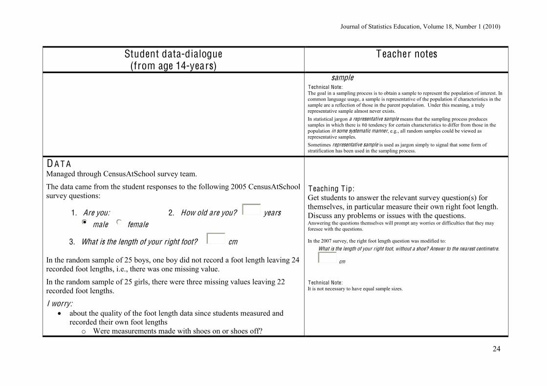
D A T A Managed through CensusAtSchool survey team.

The data came from the student responses to the following 2005 CensusAtSchool survey questions:

1. Are you: 2. How old are you? years male female

3. What is the length of your right foot? cm

In the random sample of 25 boys, one boy did not record a foot length leaving 24 recorded foot lengths, i.e., there was one missing value.

In the random sample of 25 girls, there were three missing values leaving 22 recorded foot lengths.

I worry: about the quality of the foot length data since students measured and

recorded their own foot lengths o Were measurements made with shoes on or shoes off?

T eaching T ip: Get students to answer the relevant survey question(s) for themselves, in particular measure their own right foot length. Discuss any problems or issues with the questions. Answering the questions themselves will prompt any worries or difficulties that they may foresee with the questions. In the 2007 survey, the right foot length question was modified to:

What is the length of your right foot, without a shoe? Answer to the nearest centimetre.

cm

T echnical Note: It is not necessary to have equal sample sizes.


25


T eacher notes

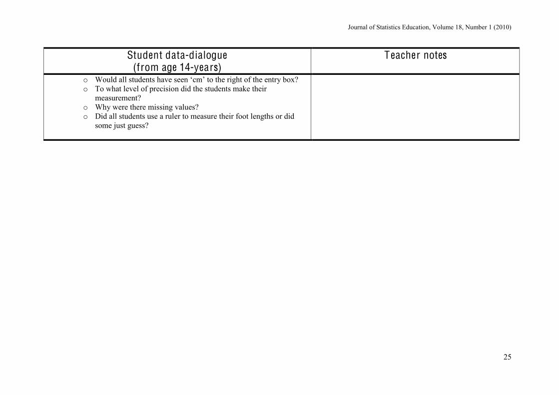
o Would all students have seen ‘cm’ to the right of the entry box? o To what level of precision did the students make their

measurement? o Why were there missing values? o Did all students use a ruler to measure their foot lengths or did

some just guess?

26


T eacher Notes

A N A L YSIS

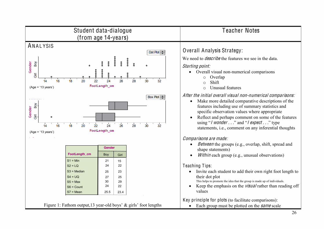
Figure 1: Fathom output,13 year-old boys’ & girls’ foot lengths

Overall Analysis Strategy: We need to describe the features we see in the data.

Starting point: Overall visual non-numerical comparisons

o Overlap o Shift o Unusual features

After the initial overall visual non-numerical comparisons: Make more detailed comparative descriptions of the

features including use of summary statistics and specific observation values where appropriate

Reflect and perhaps comment on some of the features using “I wonder . . .” and “I expect . . .” type statements, i.e., comment on any inferential thoughts

Comparisons are made:

Between the groups (e.g., overlap, shift, spread and shape statements)

Within each group (e.g., unusual observations) T eaching T ips:

Invite each student to add their own right foot length to their dot plot This helps to promote the idea that the group is made up of individuals.

Keep the emphasis on the visual rather than reading off values

K ey principle for plots (to facilitate comparisons):

Each group must be plotted on the same scale

(Age = ‘13 years’)

(Age = ‘13 years’)

Row Summary Girl

Gender

Boy FootLength_cm

21 24

25

27 30 24

25.5

15 22

23

25 29 22

23.4

15 23

24.5

27 30 46

24.5

S1 = Min S2 = LQ

S3 = Median

S4 = UQ S5 = Max S6 = Count S7 = Mean

27


T eacher Notes

T echnical Note: Dot plots:

preserve the idea that the group is made up of individuals keep the idea that we are talking about data to the forefront show the shape of the distribution (e.g., modes, skewness, subgroups) of the data suggest the shape of the underlying (population) distribution

Box plots: allow for quick visual comparisons allow for approximate reading of summary statistics (detailed reading of values

from plots should not be a major focus) obscure the individual which may increase the risk of students treating the boxes as

pictures or mistakenly interpreting the areas of segments of the box using their fraction knowledge or histogram frequency knowledge

give limited information about the shape of the distribution (symmetry/skewness) of the sample data or population

don’t show modality are not good for summarising small samples (n ≤ 15 or so)

Overall visual comparisons

I notice: there is a lot of overlap between the boys’ and girls’ foot lengths the boys’ foot lengths are shifted further up the scale one of the girls has a recorded foot length far shorter than any other girl

T eaching T ip: Ensure students know what is meant by ‘overlap’

Perhaps best explained to students visually, e.g., moving dot or box plots around on whiteboard or paper .

Shift and overlap

I notice: the middle 50% of the boys’ foot lengths (the box) is shifted much further along the scale than the middle 50% of the girls’

there is some overlap for the middle 50% of the boys’ right foot lengths and the middle 50% of the girls’

some of the boys have bigger right foot lengths than some of the girls and vice versa

T echnical Note:

The key idea is to use a central proportion to remove the influence of the relatively few high and low values, i.e., use the central bulk of the data

The ‘50%’ central proportion ties in with the box of the box plot summary.

Summary (looking at summary statistics)

I notice: the boys’ median foot length is bigger than the girls’ median by 2cm

Use the plots and the numerical summaries to compare appropriate summary statistics. Interpret statements where

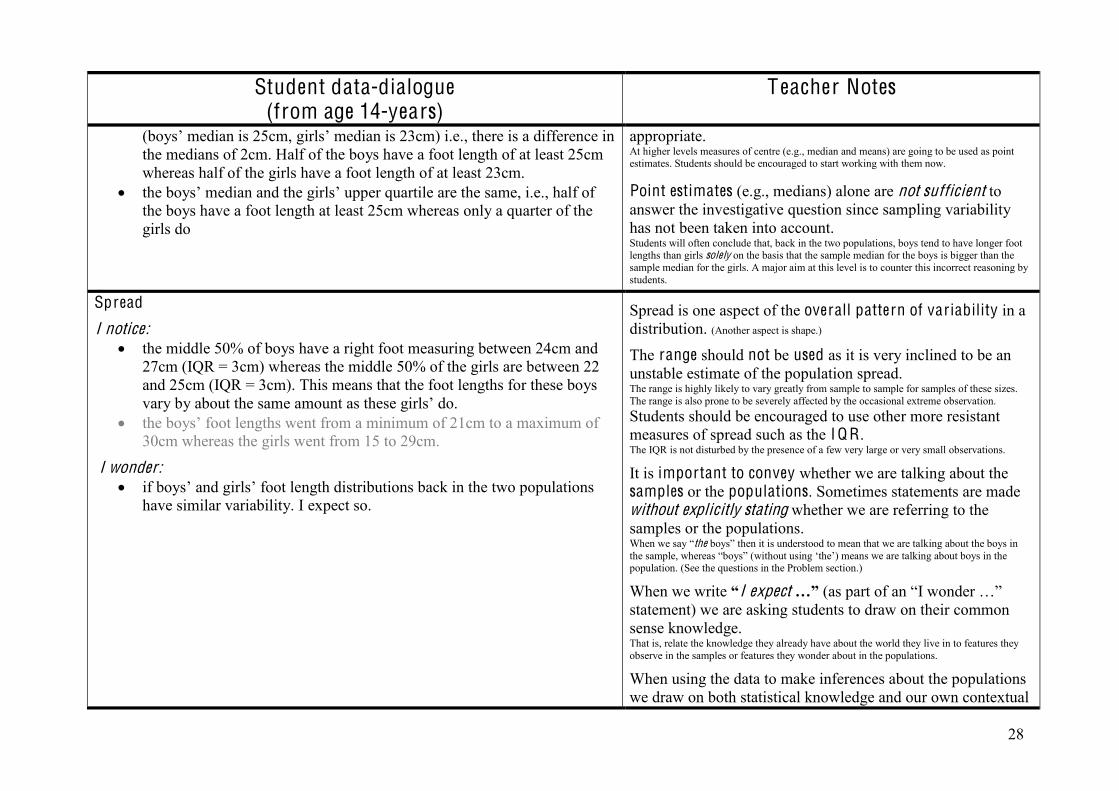
28


T eacher Notes

(boys’ median is 25cm, girls’ median is 23cm) i.e., there is a difference in the medians of 2cm. Half of the boys have a foot length of at least 25cm whereas half of the girls have a foot length of at least 23cm.

the boys’ median and the girls’ upper quartile are the same, i.e., half of the boys have a foot length at least 25cm whereas only a quarter of the girls do

appropriate. At higher levels measures of centre (e.g., median and means) are going to be used as point estimates. Students should be encouraged to start working with them now. Point estimates (e.g., medians) alone are not sufficient to answer the investigative question since sampling variability has not been taken into account. Students will often conclude that, back in the two populations, boys tend to have longer foot lengths than girls solely on the basis that the sample median for the boys is bigger than the sample median for the girls. A major aim at this level is to counter this incorrect reasoning by students.

Spread

I notice: the middle 50% of boys have a right foot measuring between 24cm and

27cm (IQR = 3cm) whereas the middle 50% of the girls are between 22 and 25cm (IQR = 3cm). This means that the foot lengths for these boys vary by about the same amount as these girls’ do.

the boys’ foot lengths went from a minimum of 21cm to a maximum of 30cm whereas the girls went from 15 to 29cm.

I wonder: if boys’ and girls’ foot length distributions back in the two populations

have similar variability. I expect so.

Spread is one aspect of the overall pattern of variability in a distribution. (Another aspect is shape.)

The range should not be used as it is very inclined to be an unstable estimate of the population spread. The range is highly likely to vary greatly from sample to sample for samples of these sizes. The range is also prone to be severely affected by the occasional extreme observation. Students should be encouraged to use other more resistant measures of spread such as the I Q R. The IQR is not disturbed by the presence of a few very large or very small observations.

It is important to convey whether we are talking about the samples or the populations. Sometimes statements are made without explicitly stating whether we are referring to the samples or the populations. When we say “the boys” then it is understood to mean that we are talking about the boys in the sample, whereas “boys” (without using ‘the’) means we are talking about boys in the population. (See the questions in the Problem section.)

When we write “I expect …” (as part of an “I wonder …” statement) we are asking students to draw on their common sense knowledge. That is, relate the knowledge they already have about the world they live in to features they observe in the samples or features they wonder about in the populations.

When using the data to make inferences about the populations we draw on both statistical knowledge and our own contextual

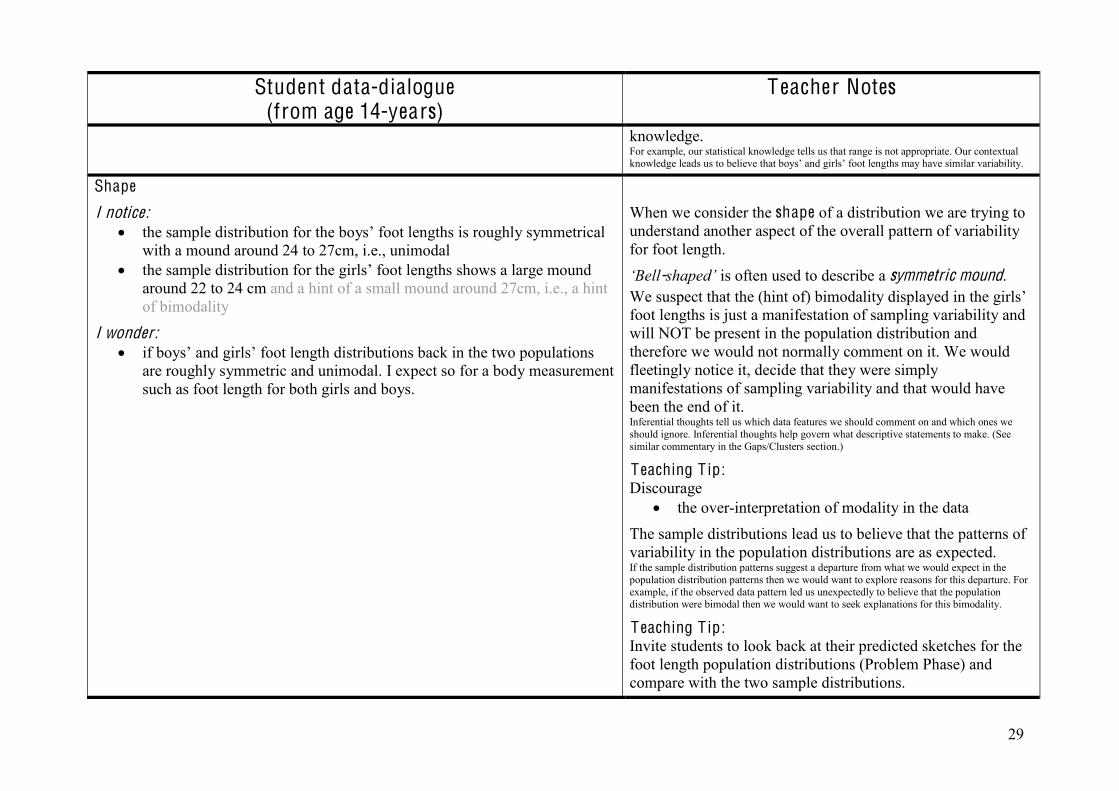
29


T eacher Notes

knowledge. For example, our statistical knowledge tells us that range is not appropriate. Our contextual knowledge leads us to believe that boys’ and girls’ foot lengths may have similar variability.

Shape

I notice: the sample distribution for the boys’ foot lengths is roughly symmetrical

with a mound around 24 to 27cm, i.e., unimodal the sample distribution for the girls’ foot lengths shows a large mound

around 22 to 24 cm and a hint of a small mound around 27cm, i.e., a hint of bimodality

I wonder: if boys’ and girls’ foot length distributions back in the two populations

are roughly symmetric and unimodal. I expect so for a body measurement such as foot length for both girls and boys.

When we consider the shape of a distribution we are trying to understand another aspect of the overall pattern of variability for foot length.

‘Bell-shaped’ is often used to describe a symmetric mound. We suspect that the (hint of) bimodality displayed in the girls’ foot lengths is just a manifestation of sampling variability and will NOT be present in the population distribution and therefore we would not normally comment on it. We would fleetingly notice it, decide that they were simply manifestations of sampling variability and that would have been the end of it. Inferential thoughts tell us which data features we should comment on and which ones we should ignore. Inferential thoughts help govern what descriptive statements to make. (See similar commentary in the Gaps/Clusters section.)

T eaching T ip: Discourage

the over-interpretation of modality in the data The sample distributions lead us to believe that the patterns of variability in the population distributions are as expected. If the sample distribution patterns suggest a departure from what we would expect in the population distribution patterns then we would want to explore reasons for this departure. For example, if the observed data pattern led us unexpectedly to believe that the population distribution were bimodal then we would want to seek explanations for this bimodality.

T eaching T ip: Invite students to look back at their predicted sketches for the foot length population distributions (Problem Phase) and compare with the two sample distributions.

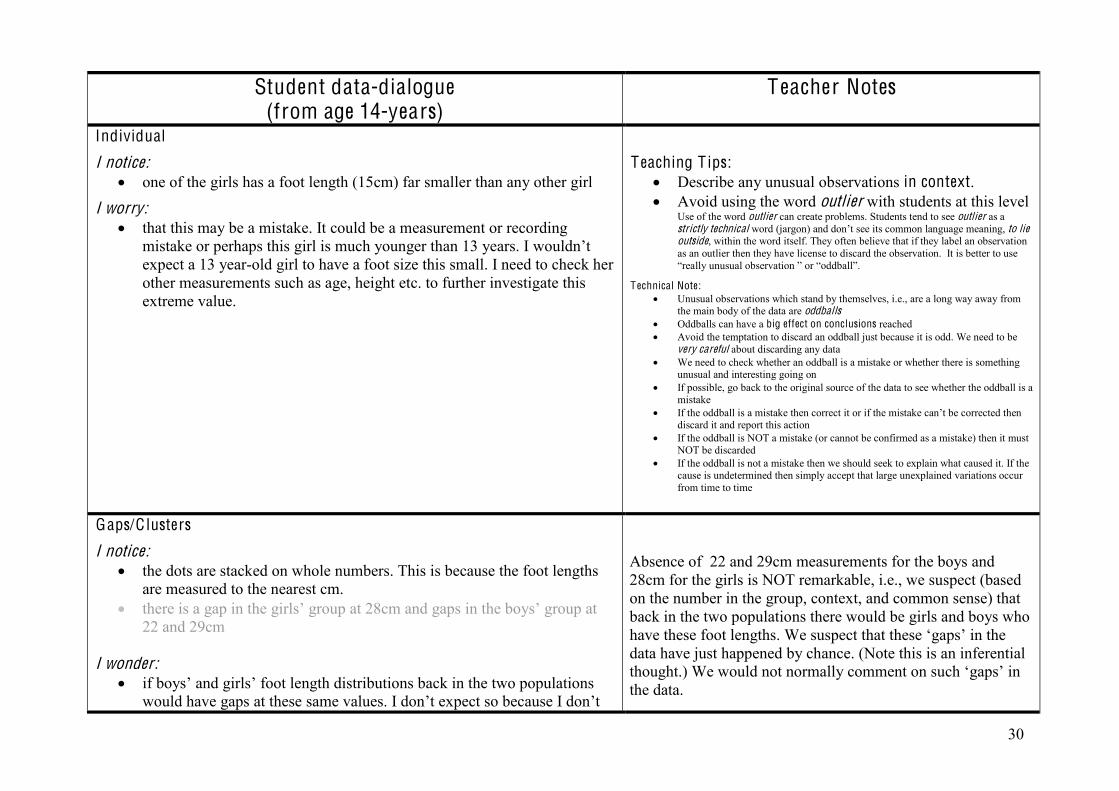
30


T eacher Notes

Individual

I notice: one of the girls has a foot length (15cm) far smaller than any other girl

I worry: that this may be a mistake. It could be a measurement or recording mistake or perhaps this girl is much younger than 13 years. I wouldn’t expect a 13 year-old girl to have a foot size this small. I need to check her other measurements such as age, height etc. to further investigate this extreme value.

T eaching T ips: Describe any unusual observations in context. Avoid using the word outlier with students at this level

Use of the word outlier can create problems. Students tend to see outlier as a strictly technical word (jargon) and don’t see its common language meaning, to lie outside, within the word itself. They often believe that if they label an observation as an outlier then they have license to discard the observation. It is better to use “really unusual observation ” or “oddball”.

T echnical Note: Unusual observations which stand by themselves, i.e., are a long way away from

the main body of the data are oddballs Oddballs can have a big effect on conclusions reached Avoid the temptation to discard an oddball just because it is odd. We need to be

very careful about discarding any data We need to check whether an oddball is a mistake or whether there is something

unusual and interesting going on If possible, go back to the original source of the data to see whether the oddball is a

mistake If the oddball is a mistake then correct it or if the mistake can’t be corrected then

discard it and report this action If the oddball is NOT a mistake (or cannot be confirmed as a mistake) then it must

NOT be discarded If the oddball is not a mistake then we should seek to explain what caused it. If the

cause is undetermined then simply accept that large unexplained variations occur from time to time

Gaps/Clusters

I notice: the dots are stacked on whole numbers. This is because the foot lengths

are measured to the nearest cm. there is a gap in the girls’ group at 28cm and gaps in the boys’ group at

22 and 29cm I wonder:

if boys’ and girls’ foot length distributions back in the two populations would have gaps at these same values. I don’t expect so because I don’t

Absence of 22 and 29cm measurements for the boys and 28cm for the girls is NOT remarkable, i.e., we suspect (based on the number in the group, context, and common sense) that back in the two populations there would be girls and boys who have these foot lengths. We suspect that these ‘gaps’ in the data have just happened by chance. (Note this is an inferential thought.) We would not normally comment on such ‘gaps’ in the data.

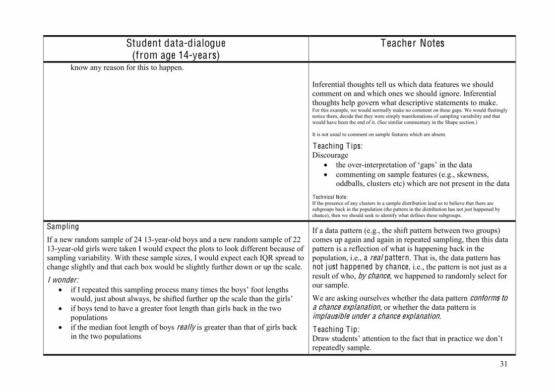
31


T eacher Notes

know any reason for this to happen.

Inferential thoughts tell us which data features we should comment on and which ones we should ignore. Inferential thoughts help govern what descriptive statements to make. For this example, we would normally make no comment on these gaps. We would fleetingly notice them, decide that they were simply manifestations of sampling variability and that would have been the end of it. (See similar commentary in the Shape section.) It is not usual to comment on sample features which are absent.

T eaching T ips: Discourage

the over-interpretation of ‘gaps’ in the data commenting on sample features (e.g., skewness,

oddballs, clusters etc) which are not present in the data T echnical Note: If the presence of any clusters in a sample distribution lead us to believe that there are subgroups back in the population (the pattern in the distribution has not just happened by chance), then we should seek to identify what defines these subgroups.

Sampling

If a new random sample of 24 13-year-old boys and a new random sample of 22 13-year-old girls were taken I would expect the plots to look different because of sampling variability. With these sample sizes, I would expect each IQR spread to change slightly and that each box would be slightly further down or up the scale.

I wonder: if I repeated this sampling process many times the boys’ foot lengths would, just about always, be shifted further up the scale than the girls’

if boys tend to have a greater foot length than girls back in the two populations

if the median foot length of boys really is greater than that of girls back in the two populations

If a data pattern (e.g., the shift pattern between two groups) comes up again and again in repeated sampling, then this data pattern is a reflection of what is happening back in the population, i.e., a real pattern. That is, the data pattern has not just happened by chance, i.e., the pattern is not just as a result of who, by chance, we happened to randomly select for our sample.

We are asking ourselves whether the data pattern conforms to a chance explanation, or whether the data pattern is implausible under a chance explanation.

T eaching T ip: Draw students’ attention to the fact that in practice we don’t repeatedly sample.

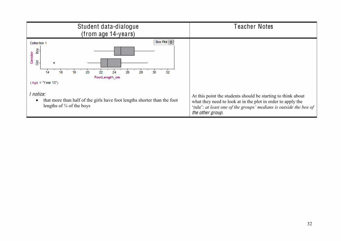
32


T eacher Notes

I notice:

that more than half of the girls have foot lengths shorter than the foot lengths of ¾ of the boys

At this point the students should be starting to think about what they need to look at in the plot in order to apply the ‘rule’: at least one of the groups’ medians is outside the box of the other group.

33


T eacher Notes

C O N C L USI O N The shift in these two samples makes me want to claim that right foot lengths of 13 year-old New Zealand tend to be longer than right foot lengths of 13 year-old New Zealand girls back in the two populations. I am prepared to make this call because, in my data, the difference between the boys’ and the girls’ foot lengths is big enough for my two sample sizes. To make this call, with sample sizes between 20 and 40, the rule requires that more than half of the girls’ foot lengths must be smaller than ¾ of the boys’ (or more than half of the boys’ foot lengths must be longer than ¾ of the girls’), i.e., the median foot length for the girls must be outside the box for the boys.

By making the call, I am saying that, in my data, the pattern of the boys tending to have longer foot lengths than the girls is not just due to who happened to be randomly selected in the girls’ group and who happened to be randomly selected in the boys’ group, i.e., has not just happened by chance. I claim that this pattern in the data is real, i.e., that this pattern persists back in the two populations.

We use ‘… right foot lengths …’ because the investigative question asks about the right foot length.

Using statistics there is always the possibility that the calls (decisions) that we make are wrong, i.e., we are making calls in the face of uncertainty. For example, we want to make a call on who tends to be taller (back in the two populations), 13 year-old boys or 13 year-old girls. We may make the call that it’s 13 year-old boys when in fact it’s girls who tend to be taller. Or, we may not want to make a call even though boys tend to be taller than girls. T echnical Note:

Making a call versus making a claim versus making a conclusion At this level we prefer to use the phrase making a call because it has a strong connotation of making a decision through a weighing-up or an on-balance type reasoning and, inherent in that, is the possibility of the ‘call’ being wrong. The phrase making a claim has, albeit to a slightly lesser extent, the same connotation. The phrase I conclude has greater connotations of certainty and therefore its use, at this level, runs the risk of the students losing sight of the fact any so called ‘conclusions’ are made in the face of uncertainty.

Explanatory

I expected boys to have bigger feet than girls. This study gives me enough information to be able to make the call that 13 year-old boys tend to have bigger feet than 13 year-old girls.

I can’t think of any other factor which can explain the difference in foot size other than gender.

In this explanatory element we ask ourselves if our conclusion makes sense with what we know, i.e., whether our contextual knowledge matches our conclusions.

We must try to think of other factors which may lead to alternative explanations when measuring foot lengths. These suggestions should also be present in the conclusion. As another example, samples from the NZ Year 5 to Year 10 Census At School database may lead us to claim that students who own a cell phone tend to have less hours of sleep per night than students who don’t. However, the explanation for the number of hours slept per night might not be cell phone ownership but rather the age of the students. That is, those students who own cell phones tend to be older students and older students tend to sleep less.

Sometimes we will not be able to think of any other factors that should be taken into account and we simply say that.

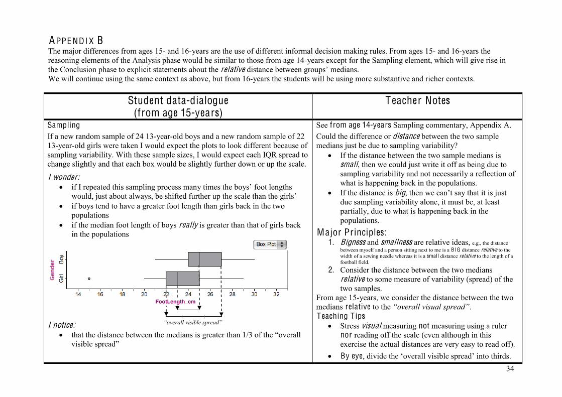
34

APPE NDI X B The major differences from ages 15- and 16-years are the use of different informal decision making rules. From ages 15- and 16-years the reasoning elements of the Analysis phase would be similar to those from age 14-years except for the Sampling element, which will give rise in the Conclusion phase to explicit statements about the relative distance between groups’ medians. We will continue using the same context as above, but from 16-years the students will be using more substantive and richer contexts.


T eacher Notes

Sampling If a new random sample of 24 13-year-old boys and a new random sample of 22 13-year-old girls were taken I would expect the plots to look different because of sampling variability. With these sample sizes, I would expect each IQR spread to change slightly and that each box would be slightly further down or up the scale.



if the median foot length of boys really is greater than that of girls back in the populations

I notice:

that the distance between the medians is greater than 1/3 of the “overall visible spread”

See from age 14-years Sampling commentary, Appendix A. Could the difference or distance between the two sample medians just be due to sampling variability?

If the distance between the two sample medians is small, then we could just write it off as being due to sampling variability and not necessarily a reflection of what is happening back in the populations.

If the distance is big, then we can’t say that it is just due sampling variability alone, it must be, at least partially, due to what is happening back in the populations.

Major Principles: 1. Bigness and smallness are relative ideas, e.g., the distance

between myself and a person sitting next to me is a BIG distance relative to the width of a sewing needle whereas it is a small distance relative to the length of a football field.

2. Consider the distance between the two medians relative to some measure of variability (spread) of the two samples.

From age 15-years, we consider the distance between the two medians relative to the “overall visual spread”. T eaching T ips

Stress visual measuring not measuring using a ruler nor reading off the scale (even although in this exercise the actual distances are very easy to read off).

By eye, divide the ‘overall visible spread’ into thirds.

“overall visible spread”

FootLength_cm

35


T eacher Notes

C O N C L USI O N I am going to claim that the right foot lengths of 13 year-old New Zealand boys tend to be longer than the right foot lengths of 13 year-old New Zealand girls back in the two populations. I am prepared to make this call because, in my data, the distance between the boys’ and the girls’ median foot lengths is big relative to the overall visible spread. To make this call, with sample sizes of around 30, the difference between the two foot length medians needs to be more than about 1/3 of the overall visible spread. This is true for my data.

I don’t believe that the pattern in my data of the boys tending to have longer foot lengths than the girls is just due to who happened to be randomly selected in the girls’ group and who happened to be randomly selected in the boys’ group, i.e., I don’t believe this data pattern has just happened by chance. I am prepared to claim that this pattern in the data is real, i.e., that this pattern persists back in the two populations.

See from age 14-years Conclusion commentary, Appendix A.

Explanatory

I expected that boys tend to have bigger feet than girls back in the populations and the information I collected (my data) supports this belief.


See from age 14-years Explanatory commentary, Appendix A.

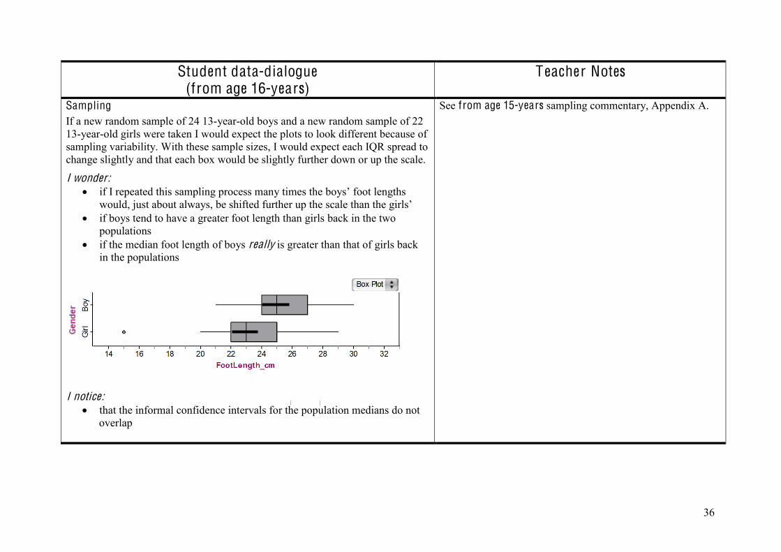
36


T eacher Notes

Sampling If a new random sample of 24 13-year-old boys and a new random sample of 22 13-year-old girls were taken I would expect the plots to look different because of sampling variability. With these sample sizes, I would expect each IQR spread to change slightly and that each box would be slightly further down or up the scale.



if the median foot length of boys really is greater than that of girls back in the populations

I notice:

that the informal confidence intervals for the population medians do not overlap

See from age 15-years sampling commentary, Appendix A.

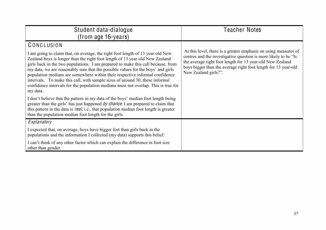
37


T eacher Notes

C O N C L USI O N I am going to claim that, on average, the right foot length of 13 year-old New Zealand boys is longer than the right foot length of 13 year-old New Zealand girls back in the two populations. I am prepared to make this call because, from my data, we are reasonably sure that the possible values for the boys’ and girls population medians are somewhere within their respective informal confidence intervals. To make this call, with sample sizes of around 30, these informal confidence intervals for the population medians must not overlap. This is true for my data.

I don’t believe that the pattern in my data of the boys’ median foot length being greater than the girls’ has just happened by chance. I am prepared to claim that this pattern in the data is real, i.e., that population median foot length is greater than the population median foot length for the girls.

At this level, there is a greater emphasis on using measures of centres and the investigative question is more likely to be “Is the average right foot length for 13 year-old New Zealand boys bigger than the average right foot length for 13 year-old New Zealand girls?”.

Explanatory

I expected that, on average, boys have bigger feet than girls back in the populations and the information I collected (my data) supports this belief.


38

Maxine Pfannkuch Department of Statistics The University of Auckland Auckland, New Zealand [email protected] +64 9 923 8794 Matt Regan Department of Statistics The University of Auckland Auckland, New Zealand [email protected] Chris Wild Department of Statistics The University of Auckland Auckland, New Zealand [email protected] Nicholas J. Horton Smith College Northampton, MA, USA [email protected]

Volume 18 (2010) | Archive | Index | Data Archive | Resources | Editorial Board | Guidelines for Authors | Guidelines for Data Contributors | Home Page | Contact JSE | ASA Publications

http://www.amstat.org/publications/

mailto:[email protected]




http://www.amstat.org/publications/jse/contents_2010.htm

http://www.amstat.org/publications/jse/jse_archive.htm

http://www.amstat.org/publications/jse/jse_index.htm

http://www.amstat.org/publications/jse/jse_data_archive.htm

http://www.amstat.org/publications/jse/jse_info_service.htm

http://www.amstat.org/publications/jse/jse_board.htm

http://www.amstat.org/publications/jse/jse_author_info.htm

http://www.amstat.org/publications/jse/jse_data_contributor_info.htm

http://www.amstat.org/publications/jse/jse_data_contributor_info.htm

http://www.amstat.org/publications/jse/.%20/


Telling Data Stories: Essential Dialogues for ... Data Stories: Essential Dialogues for Comparative...

Documents

Transcript of Telling Data Stories: Essential Dialogues for ... Data Stories: Essential Dialogues for Comparative...