Telecom Environment - Worcester Polytechnic Institute · The telecom model browser presents a...

Chapter 3Telecom Environment

The telecom modeling facilities in the netWorks application were originally designedto investigate performance issues in connection-oriented networks, such as a tele-phone network. The focus was on simulating and measuring transmission impair-ments such as transmission delay, noise, and error rates [Bell Labs 1983] and thesimulated traffic generation functions were fairly basic. The application has beenenhanced to address issues of network capacity, reliability, and availability, and thetraffic generators have been improved as well.

In a typical telecom modeling scenario you have various geographic locations withstation equipment (telsets, faxes, and so forth) interconnected through a switchednetwork. You create a model network in the drawing panel using telecom equip-ment models and then, using the Attribute palette, select the performance attributesyou want to investigate in your simulation. You must also identify the paths throughyour model that are of interest; depending on the size and scope of your model net-work, a subset of paths may be more appropriate for your simulation than studyingall possible paths. Once the path identification is completed, you can start generatingsimulated traffic over your model network and begin collecting data.

Telecom Equipment Models

Models and Systems

As discussed in Chapter??, “??,” there are two types of equipment models in net-Works—simple and compound. To be consistent with telecom terminology, com-pound equipment models are referred to assystemsin the telecom environment. Asystem configuration may be fairly simple like the Echo Canceler model or a bit moredetailed like the Digital Tandem Switching System. See Figure 3.1.

16 � Chapter 3. Telecom Environment

Figure 3.1. Telecom System Examples

As mentioned in Chapter??, “??,” only simple equipment models have attributesassociated with them and only simple equipment models can be connected by arcs.The primary purpose of systems (compound models) is to speed the model networkcreation process and add visual cues to the network representation.

Both families of simple equipment models and systems employ the notions of hierar-chy and inheritance. These hierarchies can be represented as trees, with the simplermodels serving as building blocks for the more detailed models. Figure 3.2 shows thesimple equipment model hierarchy.

SAS OnlineDoc: Version 8

Models and Systems � 17

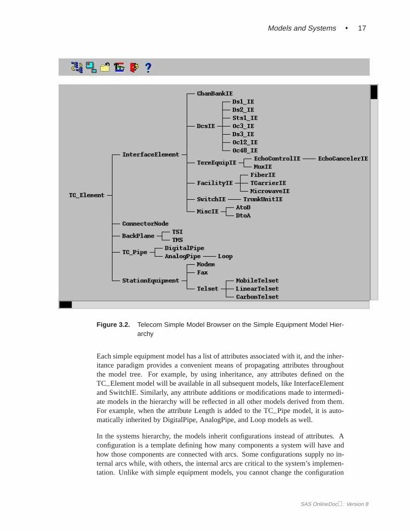
Figure 3.2. Telecom Simple Model Browser on the Simple Equipment Model Hier-archy

Each simple equipment model has a list of attributes associated with it, and the inher-itance paradigm provides a convenient means of propagating attributes throughoutthe model tree. For example, by using inheritance, any attributes defined on theTC–Element model will be available in all subsequent models, like InterfaceElementand SwitchIE. Similarly, any attribute additions or modifications made to intermedi-ate models in the hierarchy will be reflected in all other models derived from them.For example, when the attribute Length is added to the TC–Pipe model, it is auto-matically inherited by DigitalPipe, AnalogPipe, and Loop models as well.

In the systems hierarchy, the models inherit configurations instead of attributes. Aconfiguration is a template defining how many components a system will have andhow those components are connected with arcs. Some configurations supply no in-ternal arcs while, with others, the internal arcs are critical to the system’s implemen-tation. Unlike with simple equipment models, you cannot change the configuration



of a system—the location of a system in the systems hierarchy determines its config-uration. The default systems hierarchy is shown in Figure 3.3.

Figure 3.3. Telecom Systems Browser on the Systems Configurations Hierarchy


Browsers � 19

Two-Wire versus Four-Wire Equipment

In real telecommunication networks, some equipment uses the same wiring to trans-mit and receive information while other equipment might require separate wiring fortransmitting and receiving data. This distinction is commonly referred to as two-wireversus four-wire equipment. An ordinary telephone set is an example of a two-wirepiece of equipment whereas a lightwave carrier system is a four-wire facility.

These distinctions are carried through in the netWorks application. Two types of arcsare provided to accommodate bidirectional and unidirectional traffic between equip-ment models. And while it is the your responsibility to provide the right type of arcbetween models, in some cases netWorks will try to help you make the right choice.The wrong type of arc between equipment models will affect the path generationprocess discussed in the “Paths” section.

Browsers

Given the multitude and proliferation of telecommunications equipment in the mar-ketplace, it is virtually impossible for any tool to enumerate all your networking op-tions, let alone provide models for all available equipment. The netWorks applicationinstead provides models for generic categories of equipment and systems models thatyou can modify and extend to meet your needs. You can create your own permanentequipment models or systems models, or you can edit existing models using the tele-com equipment browsers. The model and system browsers are accessible through thedrawing panel pop-up menu.

The telecom model browser presents a hierarchical view of all the default simpleequipment models available in the application. (See Figure 3.2.) Using its pop-upmenu, you can invoke routines for editing the default attributes associated with amodel or create a new model derived from one of the existing models. You can useyour new or modified equipment models in your model network as soon as you exitthe browser, or you can save your changes in a SAS data set for use in subsequent net-Works sessions. Most often you will use the equipment model browser in conjunctionwith the systems browser.

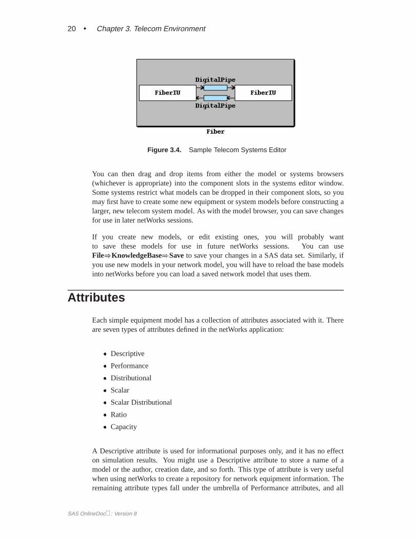
The systems browser also displays its information using a hierarchical format (seeFigure 3.3), and you create new systems using a routine similar to that in the sim-ple equipment models browser. However, the editing process for a system model isvery different from a simple equipment model. As mentioned earlier, a system modelenforces a predefined component configuration; that is, the system has well-definedpositions for holding specific types of models. To modify the default componentsin a system model, you first invoke the Edit routine on the system model in the sys-tems browser through its pop-up menu. This generates a new window displaying theconfiguration of that system. (See Figure 3.4.)



Figure 3.4. Sample Telecom Systems Editor

You can then drag and drop items from either the model or systems browsers(whichever is appropriate) into the component slots in the systems editor window.Some systems restrict what models can be dropped in their component slots, so youmay first have to create some new equipment or system models before constructing alarger, new telecom system model. As with the model browser, you can save changesfor use in later netWorks sessions.

If you create new models, or edit existing ones, you will probably wantto save these models for use in future netWorks sessions. You can useFile)KnowledgeBase)Saveto save your changes in a SAS data set. Similarly, ifyou use new models in your network model, you will have to reload the base modelsinto netWorks before you can load a saved network model that uses them.

Attributes

Each simple equipment model has a collection of attributes associated with it. Thereare seven types of attributes defined in the netWorks application:

� Descriptive

� Performance

� Distributional

� Scalar

� Scalar Distributional

� Ratio

� Capacity

A Descriptive attribute is used for informational purposes only, and it has no effecton simulation results. You might use a Descriptive attribute to store a name of amodel or the author, creation date, and so forth. This type of attribute is very usefulwhen using netWorks to create a repository for network equipment information. Theremaining attribute types fall under the umbrella of Performance attributes, and all


Distributional Attribute � 21

of these have some form of numeric value(s) associated with them. These attributescan have an impact on your network simulation results. The primary difference be-tween the various types of Performance attributes is how their associated numericvalues are calculated. The following sections present a brief synopsis of the familyof Performance attributes.

Performance Attribute

The Performance attribute provides the base for the entire family of Performanceattributes. In addition to its name, it stores four pieces of information about theattribute:

� minimum value(lowest possible numeric value allowed)

� maximum value(largest possible numeric value allowed)

� current value

� concatenation rule(algorithm to "add" two attributes of this type)

A Performance attribute returns the number stored in its current value slot when youretrieve the attribute’s value. You have to manually edit a Performance attribute tochange its current value. The minimum and maximum value numbers are used asconstraints when you edit the current value slot.

The default Performance attributes in the netWorks application are

� Constant (default:1)

� Cost (default:1)

� Loss (default:0)

� C–NotchNoise (default:0, max:95)

� Length (default:0)

� ROLR (default:0)

� TOLR (default:0)

� Capacity (min:0, max:10000)

� CallsAttempted (default:0)

� CallsBlocked (default:0)

The definitions for the specific attributes can be found in [Bell Labs 1983], [Fennick1988], and [Bell Labs 1982].



Distributional Attribute

A Distributional attribute stores a statistical distribution as well as all the Performanceattribute information. When a model queries the value of a Distributional attribute,it samples from its statistical distribution and returns that value, subject to its mini-mum value and maximum value constraints. The statistical distributions available innetWorks are described in Appendix??, “??,”.

The default Distributional attributes in the netWorks application are

� C–MsgNoise (default:Exponential(1), max:90)

� BitErrorRate (default:Exponential(1))

� BlockErrorRate (default:Exponential(1))

� ErrorFreeSeconds (default:Exponential(1))

� TimeToFailure (default:Exponential(10000))

� TimeToRestore (default:Exponential(1))

� CallHoldingTime (default:Exponential(1))

� InterCallTime (default:Exponential(1))

Scalar Attribute

A Scalar attribute uses the value of another attribute,factor, as well as the value itstores in its current value slot to compute the value to return upon a query. That is,when a Scalar attribute gets a request for its value, it first retrieves the value fromsome other attribute (factor) and then returns the product of this number and thenumber stored in its current value slot. A common use of this type of attribute is whenan equipment model has an attribute named Length associated with it. For example,the transmission delay associated with a lightwave facility could be calculated usinga Scalar attribute that stores a delay per kilometer value and uses it along with thevalue of the Length attribute to calculate the total transmission delay for the facility.In this case, the value of factor would be Length.

Scalar Distributional Attribute

A Scalar Distributional attribute combines the functionality of a Scalar and Distri-butional attribute. When it is queried for its value, a Scalar Distributional attributereturns the product of some other attribute (factor) and a sample from its own statis-tical distribution.

The default Scalar Distributional attributes in the netWorks application are

� AbsoluteDelay (default:Exponential(1), factor:Constant)


Browser � 23

Ratio Attribute

A Ratio attribute has two other attribute names associated with it. When you querythe value of a Ratio attribute, it retrieves the values of these two attributes and returnsthe result of dividing the first attribute value by the second attribute value.

The default Ratio attribute in the netWorks application is

� BlockingRate (numerator:CallsBlocked, denominator:CallsAttempted)

Capacity Attribute

A Capacity attribute also uses another attribute to determine the value it returns uponquery. This type of attribute retrieves the value of another attribute, along with theother attribute’s maximum value, and returns the result of their division.

The default Capacity attribute in the netWorks application is

� Utilization (factor:Capacity)

Concatenation Rules

Simple addition is not always the appropriate technique to “add” two values fromattributes of the same type together. Concatenation rules provide algorithms to addvarious types of attributes. The five attribute concatenation rules available in net-Works are as follows:

� Sum (+)r = a1 + a2

� PowerSum (� )r = 10 � log10(10

a1

10 + 10a2

10 )

� NegPowerSum ( )

r = �10 � log10(10�a1

10 + 10�a2

10 )

� LengthFactorr = a1 + (a2 � Length)

� NoiseLossr = (noise1 � noise2)� loss2

Browser

As with the telecom equipment models, you may need attributes other than those al-ready provided in the netWorks application, or the default values for a given attribute



may not be appropriate for your simulation. You can modify existing attributes, orcreate new ones, using the Attribute registry browser. It is accessible with the drawingpanel pop-up menu, and it is shown in Figure 3.5. Its usage is fairly straightforward.

Figure 3.5. Attribute Registry Browser

Building a Telecom Network Model

You build a telecom network model as described in Chapter??, “??,” ensuring thatfour-wire and two-wire equipment models are connected with the appropriate typesof arcs. The Telecom Equipment palette (Figure 3.6) provides quick access to someof the more commonly used telecom models.


Paths � 25

Figure 3.6. Telecom Palette

If your network model will be used for simulation purposes (as opposed to docu-mentation purposes only), it is important to include station equipment models (forexample, telsets) in your network model. These models provide the primary trafficgenerators for a simulation. (More on traffic generation in the “Traffic Generators”section.)

Running a Telecom Simulation

Before you can successfully run a simulation on your network model, the followingcriteria must be met:

� The equipment models must be connected properly.

� You must have identified which paths through the network you want to investi-gate.

� Your network model must have traffic generators.

� You must have selected attributes to be investigated during the simulation.

Paths

Path Terminology

A path in the telecom environment of netWorks is defined as an ordered series ofproperly connected equipment models with each model instance appearing only once.



Note that paths are one-directional. Any simple equipment model can be the head orsource of the path and likewise for the tail or destination. Each equipment model hasan attribute named Capacity associated with it, and any given path’s Capacity will bethe minimum Capacity value of any equipment model in the path. Equipment modelsalso have the property of beingin-serviceor out-of-service. A path is considered in-service when all of its equipment models are in-service. The netWorks applicationborrows the notions of seizing and releasing a path from telecom terminology. Beforea path can be seized, it must be available; that is, the path must be below its maximumcapacity and in-service. When a path is seized, the value of the capacity attribute foreach equipment model in the path is incremented, and when a path is released, thisvalue is decremented.

Path Generation

Before you can run a simulation in netWorks telecom environment, you must identifythe paths of interest through your network model. You accomplish this using the

Paths dialog box (Figure 3.7), which appears when you select the button inthe command panel.


Paths � 27

Figure 3.7. Paths Dialog Box

This dialog box provides two approaches for generating paths through your modelnetwork. One way is to select all of the endpoints (simple equipment models) be-tween which you want to simulate traffic and then let the netWorks identify all possi-ble pairwise paths between them. The other approach is to use the Create Path featureand select the source and destination of each path individually, then let netWorks de-termine the intermediate equipment models.

Different network models require different approaches to path generation, but themost common technique is to use endpoint selection through theCategories listbox in the Paths dialog box. You select a class (or classes) of equipment models inthe list box and then click theGenerate Pathsbutton. This creates all possible pathsbetween any instances of the selected equipment model types. A note of caution—itis possible to select any simple equipment model as a source or destination of a path,but the interpretation of the simulation results may be a bit more difficult if you do



not restrict the endpoints to similar classes of equipment (for example, all stationequipment models).

It is possible for netWorks to identify paths through a model network that could notpossibly occur in a real telecom network. For example, in Figure 3.8, there is nothingapparent that prevents the highlighted path from being generated even though it couldnever happen in a real telecom network.

Figure 3.8. Invalid Path Example

The netWorks application uses a concept ofantidromesto address this issue. The“??” section of Appendix??, “??,” provides a detailed description of antidromes andtheir usage.

Traffic Generators

When a path has been identified by the application, it attaches a traffic generator tothe source endpoint (simple equipment model) of the path. (A path would be of littlevalue to the simulation if you could not cause traffic to traverse it.) A traffic generatorgives you control over the rate at which simulated calls are generated from this sourceand also how long the calls last. If you can call multiple destinations from this source(that is, there are multiple paths from this source), you can also set the probabilitythat the call will be placed to each possible destination through the traffic generator.

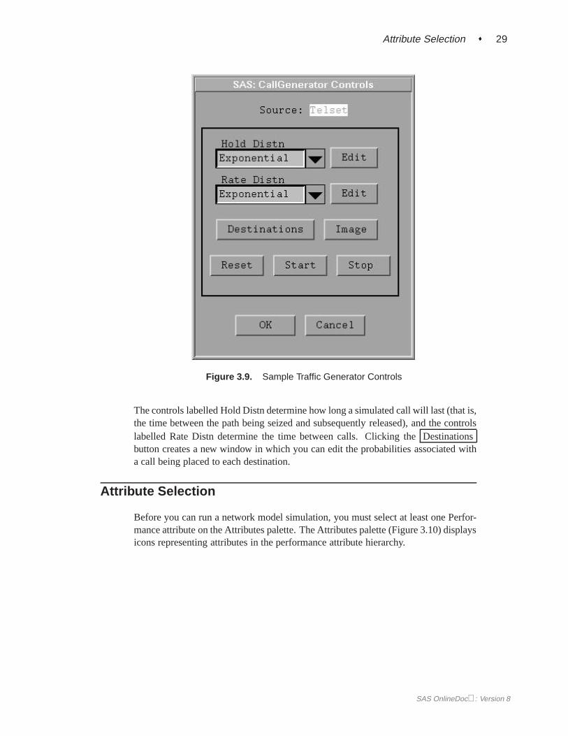
When an equipment model has a traffic generator attached to it, the Edit Attributesdialog box will have a push button for displaying the generator’s control panel. Asample traffic generator control panel is shown in Figure 3.9.


Attribute Selection � 29

Figure 3.9. Sample Traffic Generator Controls

The controls labelled Hold Distn determine how long a simulated call will last (that is,the time between the path being seized and subsequently released), and the controlslabelled Rate Distn determine the time between calls. Clicking theDestinationsbutton creates a new window in which you can edit the probabilities associated witha call being placed to each destination.

Attribute Selection

Before you can run a network model simulation, you must select at least one Perfor-mance attribute on the Attributes palette. The Attributes palette (Figure 3.10) displaysicons representing attributes in the performance attribute hierarchy.



Figure 3.10. Attributes Palette

Different icons are used to identify different types of performance attributes. For

example, is used to denote a Distributional attribute and indicates aScalar attribute. Unique icons are not yet available for Ratio or Capacity attributes.

To include an attribute in your simulation, position the cursor over the attribute’s iconand click the left mouse button. A red box appears around the icon to indicate itsselection. (Note that, even though an attribute has been selected in the Attributespalette, it is of no value to your simulation if none of the equipment models in yourpaths contain that attribute.) Once an attribute is selected (sometimes referred toasactivated), you can access the attribute’s control panel through its pop-up menu.Its control panel provides options for saving path traversal values of this attributecalculated during a simulation in a SAS data set. There is also an option to changethe size of the temporary buffer used to store the most recent values of this attributeso you can display more values in plots of this attribute.

One attribute icon in the Attributes palette always has a “$” drawn on it. This in-dicates that the attribute is being used as thecost measure when calculating paths


Animation � 31

through the network. The optimum (shortest) path between two points in a modelnetwork is the one exhibiting the lowest cost. You can change which attribute is usedas a cost attribute through the pop-up menu on the attribute’s icon.

Starting a Simulation

After the simulation paths and attributes are identified and the traffic generators arein place, you can start running the simulation; that is, you can begin generating sim-ulated traffic on your model network. There are two ways to do this.

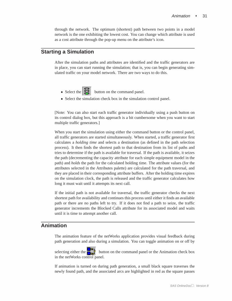
� Select the button on the command panel.

� Select the simulation check box in the simulation control panel.

[Note: You can also start each traffic generator individually using a push button onits control dialog box, but this approach is a bit cumbersome when you want to startmultiple traffic generators.]

When you start the simulation using either the command button or the control panel,all traffic generators are started simultaneously. When started, a traffic generator firstcalculates aholding timeand selects a destination (as defined in the path selectionprocess). It then finds the shortest path to that destination from its list of paths andtries to determine if the path is available for traversal. If the path is available, it seizesthe path (decrementing the capacity attribute for each simple equipment model in thepath) andholdsthe path for the calculated holding time. The attribute values (for theattributes selected in the Attributes palette) are calculated for the path traversal, andthey are placed in their corresponding attribute buffers. After the holding time expireson the simulation clock, the path is released and the traffic generator calculates howlong it must wait until it attempts its next call.

If the initial path is not available for traversal, the traffic generator checks the nextshortest path for availability and continues this process until either it finds an availablepath or there are no paths left to try. If it does not find a path to seize, the trafficgenerator increments the Blocked Calls attribute for its associated model and waitsuntil it is time to attempt another call.

Animation

The animation feature of the netWorks application provides visual feedback duringpath generation and also during a simulation. You can toggle animation on or off by

selecting either the button on the command panel or the Animation check boxin the netWorks control panel.

If animation is turned on during path generation, a small black square traverses thenewly found path, and the associated arcs are highlighted in red as the square passes


The correct bibliographic citation for this manual is as follows: SAS Institute Inc.,SAS/OR Software: The netWorks Application, Version 8, Cary, NC: SAS Institute Inc., 1999.89 pp.

SAS/OR Software: The netWorks Application, Version 8

Copyright 1999 by SAS Institute Inc., Cary, NC, USA.

ISBN 1-58025-487-X

All rights reserved. Printed in the United States of America. No part of this publication maybe reproduced, stored in a retrieval system, or transmitted, in any form or by any means,electronic, mechanical, photocopying, or otherwise, without the prior written permission ofthe publisher, SAS Institute Inc.

U.S. Government Restricted Rights NoticeUse, duplication, or disclosure of this software and related documentation by the U.S.government is subject to the Agreement with SAS Institute and the restrictions set forth inFAR 52.227-19, Commercial Computer Software - Restricted Rights (June 1987).

SAS Institute Inc., SAS Campus Drive, Cary, North Carolina 27513.

1st printing, October 1999

SAS and all other SAS Institute Inc. product or service names are registered trademarks ortrademarks of SAS Institute Inc. in the USA and other countries. indicates USAregistration.

Other brand and product names are trademarks of their respective companies.

The Institute is a private company devoted to the support and further development of itssoftware and related services.

Telecom Environment - Worcester Polytechnic Institute · The telecom model browser presents a...

Documents

Transcript of Telecom Environment - Worcester Polytechnic Institute · The telecom model browser presents a...