Techniques for Maintaining Connectivity in Wireless Ad-hoc Networks Under Energy Constraints

Techniques for Maintaining Connectivity inWireless Ad-hoc Networks UnderEnergy Constraints

FARINAZ KOUSHANFAR

Rice University

ABHIJIT DAVARE, DAVID T. NGUYEN, andALBERTO SANGIOVANNI-VINCENTELLI

University of California Berkeley

and

MIODRAG POTKONJAK

University of California Los Angeles

Distributed wireless systems (DWSs) are emerging as the enabler for next-generation wireless

applications. There is a consensus that DWS-based applications, such as pervasive computing,

sensor networks, wireless information networks, and speech and data communication networks,

will form the backbone of the next technological revolution. Simultaneously, with great economic,

industrial, consumer, and scientific potential, DWSs pose numerous technical challenges. Among

them, two are widely considered as crucial: autonomous localized operation and minimization

of energy consumption. We address the fundamental problem of how to maximize the lifetime

of the network using only local information, while preserving network connectivity. We start by

introducing the care-free sleep (CS) Theorem that provides provably optimal conditions for a node

to go into sleep mode while ensuring that global connectivity is not affected. The CS theorem is the

basis for an efficient localized algorithm that decides which nodes will go to into sleep mode and

for how long. We have also developed mechanisms for collecting neighborhood information and for

the coordination of distributed energy minimization protocols. The effectiveness of the approach is

demonstrated using a comprehensive study of the performance of the algorithm over a wide range

of network parameters. Another important highlight is the first mathematical and Monte Carlo

analysis that establishes the importance of considering nodes within a small number of hops in

order to preserve energy.

Categories and Subject Descriptors: C.3 [Special-Purpose and Application-Based Sys-tems]: Real-Time and Embedded Systems; C.2 [Computer-Communication Networks]; C.2.3

Authors’ addresses: Farinaz Koushanfar, ECE Department, Rice University, Houston, Texas 77005;

email: [email protected], Abhijit Davare, David T. Nguyen, and A. Sangiovanni-Vincentelli, EECS

Department, University of California at Berkeley, Berkeley, California 94720; Miodrag Potkonjak,

University of California at Los Angeles, Los Angeles, California 90024.

Permission to make digital or hard copies of part or all of this work for personal or classroom use is

granted without fee provided that copies are not made or distributed for profit or direct commercial

advantage and that copies show this notice on the first page or initial screen of a display along

with the full citation. Copyrights for components of this work owned by others than ACM must be

honored. Abstracting with credit is permitted. To copy otherwise, to republish, to post on servers,

to redistribute to lists, or to use any component of this work in other works requires prior specific

permission and/or a fee. Permissions may be requested from Publications Dept., ACM, Inc., 2 Penn

Plaza, Suite 701, New York, NY 10121-0701 USA, fax +1 (212) 869-0481, or [email protected]© 2007 ACM 1539-9087/2007/07-ART16 $5.00 DOI 10.1145/1275986.1275988 http://doi.acm.org/

10.1145/1275986.1275988

ACM Transactions on Embedded Computing Systems, Vol. 6, No. 3, Article 16, Publication date: July 2007.

2 • F. Koushanfar et al.

[Network Operations]: Network Management; D.4.4 [Communications Management]: Net-

work communication; D.4.7 [Organization and Design]: Distributed Systems, Real-Time Sys-

tems, and Embedded Systems

General Terms: Performance, Reliability

Additional Key Words and Phrases: Low power, sleeping coordination, connectivity, power man-

agement, energy management, ad-hoc networks

ACM Reference Format:Koushanfar, F., Davare, A,m Nguyen, D. T., Sangiovanni-Vincentelli, A., and Potkonjak,

M. 2007. Techniques for Maintaining Connectivity in Wireless Ad-hoc Networks Under

Energy Constraints. ACM Trans. Embedd. Comput. Syst. 6, 3, Article 16 (July 2007), 22 pages.

DOI = 10.1145/1275986.1275988 http://doi.acm.org/ 10.1145/1275986.1275988

1. INTRODUCTION

Wireless ad-hoc networks (WANs) are distributed embedded systems consist-ing of a large number of nodes each equipped with computational, storage,communication, and, in some cases, sensing and actuating, subsystems. WANsare widely perceived as the implementation platform of choice for numerousimportant distributed wireless systems (DWSs), such as pervasive computing,sensor networks, WWW-based information networks, and voice and multime-dia communication networks. While WANs and DWSs open up numerous, high-impact research and economic opportunities, they simultaneously pose severalnew challenging technical problems. There is wide consensus that among theseproblems, two are of dominating importance: (1) low-energy design and oper-ation, and (2) autonomous localized operation and decision making. The mosteffective method for energy minimization in DWSs is to put a large percentageof nodes into sleep mode, ensuring that the sleeping nodes are not required foraddressing the current needs.

Although there have been a number of efforts to determine the conditionsfor a node to enter sleep mode using only locally available information, whilepreserving the overall connectivity of the network, only heuristic answers havebeen presented [Xu et al. 2001; Chen et al. 2002; Cerpa and Estrin 2002]. Wepropose necessary and sufficient conditions to maintain network connectivitywhile putting a number of nodes in sleep mode. It is interesting to note that somewidely used localized heuristics do not correctly preserve network connectivity.Therefore, our main objective is to propose a fundamentally sound and effectivelocalized technique for power minimization in WANs.1

To introduce the core problem of determining when a node can go to sleepwhile maintaining the connectivity requirements, we present a small and il-lustrative example. Figures 1a and b show a part of a network. It is assumedthat nodes M , L, J , I , H, F , G, D, and N are connected to other nodes inthe network that are not shown, for the sake of simplicity. A square indicatesan awake node and a triangle denotes a sleeping node. The edge between twonodes indicates that they can communicate directly if both nodes are awake. We

1This article extends the results presented in the International Symposium on Low Power Elec-

tronic Designs [Koushanfar et al. 2003].


Techniques for Maintaining Connectivity in Wireless Ad-hoc Networks • 3

Fig. 1. Motivational figure.

assume that each node has information only about its neighbors’ existence andthe neighbors’ awake/sleep status. In this example, our goal is to determine ifnode A can go into sleep mode. Assuming that communication has a dominatingenergy cost, the objective is to contact as few nodes as possible, which limitsus to collect and use only local information. The key observation (as proved inSection 4) is that this task can be done locally: all that is needed is to check ifthere is a path through awake nodes that visits all awake neighbors of node Aand that does not contain node A. In Figure 1a, one such path is highlighted.It is interesting to note that no previous approach for this task was able tocorrectly derive this condition. In Figure 1b, there are no such paths; thus,node A should not go into sleep mode. The reason is that if node A goes to sleep,nodes C and B will become disconnected from the rest of the network. Note thatthe only difference between the two networks is that in Figure 1a node N isawake and in Figure 1b it is in sleep mode. In the rest of the paper, we demon-strate how this observation can form the basis for an efficient method to opti-mize the lifetime of a network.

2. RELATED WORK

We survey only a small sample of important efforts, mainly those whichstarted particular lines of research that have most influenced our work. Low-power research started its systematic rapid growth with two events: the firstcomprehensive set of techniques for energy modeling [Ghosh et al. 1992]and the establishment of principles for power minimization in CMOS design[Chandrakasan et al. 1992]. After that, optimization-intensive techniques havebeen first proposed for behavioral synthesis in statically scheduled systems[Chandrakasan et al. 1995]. Next, techniques have been proposed for powerminimization in systems with dynamic behavior and for operating system-levelpower programmable systems [Macii et al. 1997]. In addition, variable voltagetechniques started to gain in popularity [Yao et al. 1995; Hong et al. 1999].More recently, centralized techniques for power minimization attracted a greatdeal of attention [Simunic et al. 2001], as have several approaches that useonly local information for power management in WANs. Our goal is to exactlyaddress these limitations.

A number of power-minimization methods using a sleeping strategy wereproposed for wireless ad-hoc networks. GAF [Xu et al. 2001] is a conservativeenergy conservation scheme that superimposes a virtual grid proportional to



the communication radius of the nodes onto the network. Since nodes in onegrid block are equal from the routing perspective, the redundant nodes withina grid block can be turned off. SPAN [Chen et al. 2002] is a distributed random-ized algorithm that attempts to preserve connectivity and capacity in wirelessnetworks, but does not provide a proof of necessary and sufficient conditionsfor guaranteeing this preservation of connectivity. ASCENT [Cerpa and Estrin2002] proposes adaptive self-configuration algorithms for wireless networksthat enable online tuning of the system parameters, such as sleep time of thenodes, to extend the lifetime of the overall system. STEM [Schurgers et al.2002] suggests another power-saving strategy that does not try to preserve thecapacity of the network. STEM works by putting an increasing number of nodesinto sleep mode and then encountering the latency to set up a multihop path.Nodes in STEM must have an extra low-power radio called a paging channelthat does not go into sleep mode and constantly monitors the network to wakethe node up in cases of an interesting event.

The connected dominating set problem seeks to find a connected set withminimal cardinality with the property that each node in the network is eithera member of the set or has a neighbor that is a member of the dominating set.The dominating connected set is often used in WANs for abstracting several im-portant problems [Dai and Wu 2005; Han et al. 2004; Stojmenovic et al. 2002;Wu and Li 1999; Zheng and Kravets 2005]. The topology management underthe energy constraints is different from the problem of finding the connecteddominating set in two aspects. First, topology management is not a static prob-lem and keeps changing the set of awake nodes. The set of awake nodes arenot necessarily minimal. Second, at each point in time, the topology manage-ment under energy constraints seeks to identify the maximum number of kdisjoint connected sets in an asynchronous and localized way. The disjoint setsare selected to be placed in the sleep state.

Hence, the relationship between the two problems (i.e., topology manage-ment and minimal connected dominating set) is analogous to the relationshipbetween the maximal independent set and graph coloring. While both prob-lems are NP-complete, it is well known that it is much easier to solve maximalindependent set optimally using implicit enumeration or ILP. Also, it is wellknown that using maximal independent set iteratively to color a graph veryoften results in a very low-quality solution [Leighton 1979]. Our conjecture isthat the stated observations also hold for the relationship between the con-nected dominating set problem and the problem of maximizing the lifetime ofthe multihop wireless networks. Therefore, although connected dominating setis a very important problem in its own right and has a wide application do-main in wireless multihop networks, it is not applicable when the goal is todynamically maximize the lifetime of wireless ad-hoc networks using topologymanagement techniques.

We extend the results of the care-free sleeping theorem that we introducedbefore [Koushanfar et al. 2003]. We provide a more comprehensive set ofevaluation results and use mathematical and Monte Carlo analysis to pro-vide a deeper understanding and application range of the care-free sleepingtheorem.



3. PRELIMINARIES

3.1 Wireless Ad-hoc Networks

We assume an ad-hoc wireless network where there is no fixed infrastructure orcentralized wireless control. Because of the limited energy sources, a node onlycommunicates directly to other nodes within its short-range distance. If twonodes are not within the short-range distances of each other, they communicateusing other nodes as intermediate relays. Although we have used the short-range communication model in our simulations, our algorithm is generic in thatit can work with any communication model as long as the network is connected.The network is assumed to be fully connected initially, i.e., we assume that thereis at least one path between every two nodes in the network. Once some nodesdisappear from the network’s topology because of power depletion, the networkmight become disconnected. The communication between the nodes is in theform of local broadcasting. Also, a node that is not in the sleep state periodicallybroadcasts a POLLING messages that contains information about that node,which includes its ID, current token group (see Subsection 6.3), location, andstate (described in the energy model) along with a list of its current neighbors.Our algorithm is operating above the link layer and medium access (MAC)layers of the network, so it can take advantage of the power-saving strategiesproposed for those levels.

3.2 Energy Models

A node can be in one of the three following states. (1) A node is assumed to bein sleep state, if its radio is off and, hence, it is disconnected from the commu-nication topology graph. (2) A listening node that has its radio on, but is notusing it for communication, and is assumed to be in idle state. (3) A node that iscommunicating with other nodes using its radio is in active state. When a nodeis in active state, it can be either in transmitting or receiving state. A node canswitch its state from time to time and the energy usage of a node depends on itscurrent state. We assume an energy model where a node’s energy consumptionin sleep state is much lower than the energy consumed in other states and theidle state has energy consumption on the same order of magnitude as the activestate. We further distinguish between the energy consumed for transmissionand reception. We employ a random traffic model in our simulations for thecommunication between the nodes.

4. PROBLEM FORMULATION AND FOUNDATIONS

In this section, we present informal and formal definitions of the overall ad-dressed problem—localized WANs life-time optimization. We refer to the prob-lem as the max lifetime problem.

4.1 Problem Formulation and Complexity

An ad-hoc network with n nodes that forms a connected graph is given. Initially,each node i has an amount of energy Ei. If a node is in sleep mode, it spendsenergy Es per unit of time. If a node is in the active mode, it spends energy Ea



per unit of time. Ea is significantly higher than Es. Our goal is to maximizethe lifetime of the network in such a way that at each point of time all awakenodes can communicate to each other using multihop communication and thateach sleeping node has at least one awake neighbor. The rationale behind thefirst condition of this formulation is to allow all awake nodes to communicate.The rationale of the second condition is twofold. First, when a node wakes up,it can immediately access information that was sent to it through one of theawake neighbors. Second, if a node has to wake-up, the node can immediatelycommunicate to any awake node.

Formally the max lifetime (MLT) problem can be stated in the following way.

INSTANCE: Graph G = (V , E), function W (i), for all i elements of V , and aninteger T .

QUESTION: Is there a mapping F (i, t) to binary domain s.t. for each t eachnodes i s.t. F (i, t) = 1 have a path between them that consists only of nodes withproperty that F (i, t) = 1, and that for each node j that has F ( j , t) = 0, there isan edge to a node k that has F (k, t) = 1. In addition, for each node in the graph∑

t(F (i, t) ≤ W (i)), and t ≥ T.

Note that W (i) is the total energy at node i and the function F (i, t) indicatesthe state of node i at time t. If F (i, t) = 0 the node i is sleep at time t whereasif F (i, t) = 1, node i is awake at time t. The problem can be generalized in astraightforward way to account for wake-up cost. We have proved that the MLTproblem is an NP-complete problem by transforming the connected dominatingset problem [Garey and Johnson 1979] into a special case of the MLT problem.For the sake of brevity and because of space limitations the proof is omitted.Therefore, it is extremely unlikely that an optimal polynomial time algorithmfor the MLT problem can be developed. At the core of the MLT problem is acare-free sleep subproblem that provides the conditions that must be satisfiedbefore a node can go into sleep mode, while the connectivity of the network isstill maintained. We address this core subproblem in the next subsection.

4.2 Care-Free Sleep Theorem

We term a node that is in sleep mode as a sleeping node and a node that is intransmitter/ receiving mode as an awake node. We denote a node being con-sidered for sleep by A. We assume that when all nodes in the network areawake, they form a single connected graph. In addition, a specified number oftokens is initially generated. The number of generated tokens is smaller thanthe number of nodes in the network. The node that is the owner of a tokenis being denoted as a token node. Each token node initiates the procedure forevaluating the conditions for changing its operational mode from active intosleep state. Once the procedure is completed, the current token node passes itstoken to one of its randomly selected neighbors. Finally, we assume availabilityof a synchronization mechanism (one such protocol is presented in Section 6.3),which enforces that each node in the network is simultaneously considered by,at most, one procedure initiated by one of the concurrent tokens. Consequently,the considered neighborhood of the nodes that simultaneously have a token willbe disjoint.



Care-Free Sleep Theorem: An arbitrary node A can go into sleep if, and only if,there exists a path consisting only of awake nodes that does not contain node Aand that visits all of its awake neighbors and each of its sleeping neighbors haveat least one other awake neighbor.

PROOF. The proof is presented using a reductio ad absurdum strategy.If: Suppose that the conditions are satisfied. Note that the existence of a

path that visits all the neighboring nodes is equivalent to and therefore impliesa path between any pair of neighbors. Let us denote two arbitrary nodes inthe network by S and D. Assume that there is a path P between S and Dand that the path P is through node A. Obviously, path P is incoming to nodeA from one of its neighbors and leaving through another neighbor. We denotethese neighbors as Ni and No. After node A goes to sleep, by the conditionof the theorem, there is still a path Pio from Ni to NO that does not containA. If we replace the original subpath Ni → A → No by a subpath Pio, thelater subpath will form a path from S to D with the reminder of the path P(P \ ((Ni → A → No)). Furthermore, since each of the sleeping neighbors ofnode A has another neighbor awake, the second condition will be also satisfiedafter node A goes to sleep.

Only if: Suppose that the conditions are not satisfied. Therefore, there is apair of neighbors Ni and No that do not have path between them after the nodeA goes to sleep or there is a neighbor node Ns in sleep mode that has A as itsonly awake neighbor. The first condition implies that Ni or No (or both) will beisolated (not connected to the rest of the network) after node A goes to sleep.The second condition implies that node Ns will not have an awake neighbor.Therefore, node A must stay awake.

5. PROBABILISTIC PERFORMANCE EVALUATION

In this section, we present mathematical and Monte Carlo simulation-basedanalysis of small instances of networks that consist of a single node and a num-ber of its one-hop or small number of hops neighbors. The goal of the analysisis to evaluate and justify the applications of the care-free sleep theorem as apractical tool for selecting the eligible node for entering the sleep mode by an-alyzing the node’s small radius neighborhood. The analysis is conducted underthe assumption that the awake nodes are uniformly randomly distributed.

Therefore, the purpose of the results of this section is not to establish themathematical and simulation-based proofs that in uniformly distributed wire-less ad-hoc networks it is sufficient with a very high probability to consider onlythe two-hop neighborhood to evaluate the eligibility of one node to enter thesleep state. The objective of the section is only to provide an intuition behindthe expected size of the local search region. In many cases, one could expectthat considering only a small immediate neighborhood is sufficient to make acorrect decision for placing a particular node in the sleep state.

5.1 Mathematical Performance Analysis

In this subsection, we calculate the probability that a node can go to sleepwhen it has only two neighbors under the condition that there is a direct path



Fig. 2. Calculating the shared area between the ranges of A and B, while node B is at the distance

x(x < r) from A.

between its neighbors. Assume that we have three nodes A, B, and C, wherenode A can directly communicate with both nodes B and C. Figure 2 illustratesthis scenario. Under the stated assumptions, node A can only go into sleep modeif there is an edge between B and C, which implies that the distance between Band C is smaller than the communication range r. Therefore, our goal is to cal-culate the probability of having direct communication between nodes B and C.

We follow a uniform random distribution scheme for the placement of nodesin the area. Hence, the probability that a node exists in a given area is propor-tional to the size of the area. In order to calculate the probability that nodes Band C can directly communicate, we make two observations. The first is basedon symmetry for all points that are the same distance x from node A. All of thesepoints have the same probability of the targeted event. The second is that theprobability that node B is distance x from node A is linearly proportional to x.

Therefore, we study the case where we move node B within the range ofnode A. For each placement of node B, we calculate the area shared betweenthe communication ranges of A and B. If node C belongs to this area, thereis direct communication between nodes B and C. This area corresponds to theintersection of two circles and is the nonshaded area of the circle A in Figure 2.If we denote the intersection points of the of circles A and B by M and M ′, thenthe line M M ′ has length y that can be calculated using the following equation.

y = 2

√r2 + (x/2)2 =

√4r2 − x2 (1)

The angle � MAM ′ is denoted by α and is calculated in the following equation.

� (α/2) = arccos(x/2r)

⇒ � α = 2 arccos(x/2r) (2)

We consider the area that is shared between the circles A and Bby Area(shared). Using the calculated values for y and α, we calculateArea(shared) for each placement of B at the distance x of the node A (x < r) asfollows.

Area(M̂AM ′) = αr2/2 (3)



Area(MAM ′) = x y/4 = x√

4r2 − x2/4 (4)

Area(shared) = 2(Area(M̂AM ′) − Area(MAM ′))= 2r2 arccos(x/2r) − x

√4r2 − x2/2

The probability that an edge exists between B and C, given that node Bis distance x from node A is the same as the probability of C being in theArea(shared), given that AB = x. Since we assumed a uniform distribution ofnodes, where C can be placed anywhere within the circle A with radius r, theprobability of C being in Area(shared), given that AB = x can be calculated inthe following way.

Prob(C ∈ Area(shared)|AB = x) (5)

= Area(shared)/Area(circle)

= (2r2 arccos(x/2r) − x√

4r2 − x2/2)/πr2

In order to calculate the probability of an edge between B and C, we needto find the integral of the Prob(C ∈ Area(shared) as the node B moves withinthe range 0 to r inside the circle centered at A. This probability is calculatedas follows.

Prob(C ∈ Area(shared)) (6)

= Prob(C ∈ Area(shared)|AB = x).Prob(AB = x)

Since we follow the uniform random distribution of nodes B and C withinthe circle, we need to take the integral with respect to x.dx to transform theuniformly distributed x and y from the Cartesian coordinates to the polar coor-dinates. Therefore, we calculate the targeted integral as follows.

Prob(BC ≤ r) (7)

=∫ r

0

(2(2r2 arccos(x/2r) − x

√4r2 − x2/2)

πr4

)xdx

= 2

πr4

∫ r

0

(2r2 arccos(x/2r) − x√

4r2 − x2/2)xdx

For calculation of the integral in the Eq. (7), we used the symbolic Integratorfrom the Mathematica 4.1 software package [WolframResearch 2001]. We thenused the same package to calculate the value of the integral at each of theendpoints of the interval and, therefore, to obtain the probability of an edge be-tween the nodes B and C. The result and the probabilities are shown in Eq. (8).

Prob(BC ≤ r) (8)

= 2

πr4.

[ −2r

6√

4r2 − x2.

[3r2x

√4r2 − x2

√1 − x2/4r2

− 6r2x2

√1 − x2/4r2 arccos(x/2r)

− 12r4

√1 − x2/4r2 arcsin(x/2r)

+ x3√

4r2 − x2Hypergeometric2F1

(1.5, −0.5, 2.5,

x2

4r2

)]]r

0

= 0.5865



Fig. 3. The probability of an alternative path among the neighbors of the node A versus N, number

of neighbors of A.

Thus, if a node has two neighbors, each placed according to the uniform randomdistribution, the probability of having an edge between the two neighbors is0.5865.

5.2 Monte Carlo Performance Analysis

In order to study the cases where there are more than two nodes within therange of node A, we conduct Monte Carlo simulations. For each study, we gener-ate random instances of node A with N neighbors. The neighbors are generatedwith a uniform random distribution within the circle of communication rangeof the node A. We vary the number N from 2 to 14. For each value of N, weperform 1,000,000 simulations and gather statistics on the existence of a pathamong all the neighbors of A that does not pass through node A. The resultsare shown in Figure 3. In order to gain additional insights, we extended theMonte Carlo simulation studies in 3-dimensional (3D) space. Now the commu-nication domain of each wireless node has a spherical shape. The results forthe probability of an alternative path in 3D space are shown in Figure 4. Thekey observation is that the changes for probabilities of paths are proportionalto the probabilities obtained for the two dimensional scenarios. The only differ-ence is that now we have smaller absolute probabilities. This can be explainedby the larger average distances between the uniformly randomly distributednodes within a sphere than within a circle of identical radius. Therefore, thekey consequence is that in the 3D case it is even more important to consider thenodes outside of the communication range of a sleep candidate node to achievethe maximal lifetime of the network.

The first interesting and important observation is that for N = 2, the proba-bility of a direct path between two neighbors is 0.5859. Since the Monte Carloconverges at rate

√n, where n is the number of iterations, we expect that about

3.5 digits are correct after one million tries [Haber 1970; Rubinstein 1981].Therefore, we have full agreement with the value that was derived in Eq. (8)



Fig. 4. The probability of an alternative path among the neighbors of the node A versus N, number

of neighbor of A for 3D cases.

and full confirmation of the analysis in Subsection 5.1. The second interestingobservation is that the graph in Figure 3 is nonmonotonic and the probabil-ity of having a path between three neighbors is 0.544, which is lower thanthe probability of having a path between two neighbors. This is unexpected, atfirst glance, since it seems that there is greater probability of having a pathbetween three neighbors than between two neighbors. However, the study in-dicates that for three neighbors the probability is lower, because of the largernumber of direct paths that are needed.

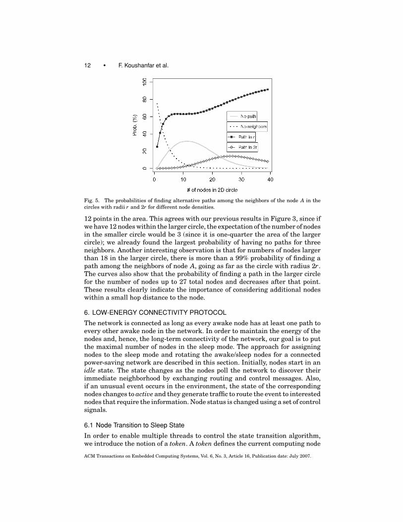
Another study that we have conducted using the Monte Carlo simulationsattempts to find the required locality of the search to determine an alternativepath among the neighbors. In this study, the deployment area is a circle withradius 2r. Node A, which has the intention of entering sleep mode, is in thecenter of this circle. The communication range of node A remains r. We varythe density of the nodes in the circle with radius 2r. For every number of nodesin the larger circle between 0 and 40, 1,000,000 experiments were run. Foreach density, we estimate the probability of finding a path that connects all theneighbors of node A and lies inside the communication range of node A. Also, foreach density, we estimate the probability of finding a path among the neighborsof node A going to the larger circle. The results are shown in Figure 5. Thedashed curve (Figure 5) indicates the probability of node A having no neighborsis very high for a low number of nodes in the 2r circle. The curve with the squarepoints shows the percentage of time the path among the neighbors can be foundin the range of node A. The curve with the empty diamond points indicates thepercentage of time we could find a path among the neighbors of node A, only byconsidering nodes in the outer circle (with the radius 2r). The last curve (theplain curve) is a function of the previous two curves and shows the percentageof time there are no paths among the neighbor nodes to node A, even aftergoing to the second circle. We can observe that the probability of an alternativepath in the smaller circle stays constant for the node densities between 5 and15. The probability of having no path is a function that has a maximum of



Fig. 5. The probabilities of finding alternative paths among the neighbors of the node A in the

circles with radii r and 2r for different node densities.

12 points in the area. This agrees with our previous results in Figure 3, since ifwe have 12 nodes within the larger circle, the expectation of the number of nodesin the smaller circle would be 3 (since it is one-quarter the area of the largercircle); we already found the largest probability of having no paths for threeneighbors. Another interesting observation is that for numbers of nodes largerthan 18 in the larger circle, there is more than a 99% probability of finding apath among the neighbors of node A, going as far as the circle with radius 2r.The curves also show that the probability of finding a path in the larger circlefor the number of nodes up to 27 total nodes and decreases after that point.These results clearly indicate the importance of considering additional nodeswithin a small hop distance to the node.

6. LOW-ENERGY CONNECTIVITY PROTOCOL

The network is connected as long as every awake node has at least one path toevery other awake node in the network. In order to maintain the energy of thenodes and, hence, the long-term connectivity of the network, our goal is to putthe maximal number of nodes in the sleep mode. The approach for assigningnodes to the sleep mode and rotating the awake/sleep nodes for a connectedpower-saving network are described in this section. Initially, nodes start in anidle state. The state changes as the nodes poll the network to discover theirimmediate neighborhood by exchanging routing and control messages. Also,if an unusual event occurs in the environment, the state of the correspondingnodes changes to active and they generate traffic to route the event to interestednodes that require the information. Node status is changed using a set of controlsignals.

6.1 Node Transition to Sleep State

In order to enable multiple threads to control the state transition algorithm,we introduce the notion of a token. A token defines the current computing node



Fig. 6. Pseudocode for the localized strategy to select nodes for standby state.

(CCN) that has the control of the power-saving procedure. Since the procedurehas a localized scope and a distributed nature, there can be multiple tokensoperating in different places in the network. The tokens are assigned to nodesand handshaking between the tokens is done using the protocol presented inSubsection 6.3. Pseudocode of the procedure for putting a node to sleep is sum-marized in Figure 6. A CCN makes an evaluation of itself and its current neigh-bor nodes in order to decide which one of them is the best choice for transition tosleep mode. As shown in Figure 6, each CCN node makes that decision for thenodes within its local neighborhood (Step 1). Before making any decisions, theprocedure has to update the information about the routes in the k-hop neighbor-hood of the CCN (Step 3). The updating is accomplished with local broadcastingto the neighbors and selective flooding to the CCN node. The procedure reservesa variable named BEST-CANDIDATE consisting of a node’s ID and its criticalenergy at the CCN and assigns the value zero to critical energy and nil to ID(Step 4). While the computation is still conducted at CCN, the procedure eval-uates CCN and each of its neighbors to determine the best candidate for thesleep state (Steps 5–17). Note that all the computation at the CCN requiresonly information from the k-hop routing table gathered in Step 3. The eval-uation process for a NODE(i) starts by computing the shortest path betweeneach pair of its neighbors using the standard Floyd–Warshall algorithm, with-out using NODE(i) on the path (Step 7). If there are pair of neighbor nodes



that do not have a path between them, NODE(i) cannot go to sleep state (Steps8–9). Otherwise, the procedure selects the pair of neighbors to the NODE(i)with the longest path between them and saves the path information in MAX-SHORTEST(i) (Steps 10–12). Next, the node with the minimum energy on theshortest path is selected as the critical node and its information is saved inCRITICAL-E(i) (Step 13). This node is critical, since alteration of its mode cancause the alternative path to become disconnected. Since the goal is to maximizethe network lifetime, if the alternative path to a sleeping node is critical withrespect to energy, that node is not a good candidate for sleep state. Therefore,BEST-CANDIDATE always stores the node with the maximum CRITICAL-E(i)(Step 18). After that, the CCN has to decide the next token node from amongits neighbors. The procedure selects an awake neighbor that has not receivedthe token for the longest time (Step 19). The CCN node then broadcasts itsdecision about the sleep transition, frees the nodes in its k-hop neighborhood,and passes the control of the procedure to the next token node (Step 20).

6.2 Sleep to Idle Transition

A node that transitions into a sleep state, sets a self-timer and remains in thisstate for Ts time units. After the interval Ts, the node wakes up and sendsPOLLING messages to the nodes in its proximity. An important parameterin the effectiveness of the algorithm is the length of sleep time for at leastthree reasons. First, the longer the sleep time Ts, the higher the power savings.Note that the transition from sleep mode to active mode is usually very energyintensive. Second, there is an uncertainty in estimating the rate of energy con-sumption of the nodes on the alternative paths, because of the nonlinearity ofbattery discharging and also the random traffic patterns in the network, and,hence, the network might become disconnected if the length of Ts is long. Third,the shorter the length of Ts, the more flexible the network is to dynamic net-work topologies (e.g., handling node mobility). We determine Ts as a functionof energy of the alternative paths to the node, the expected traffic energy con-sumption, and the length of the alternative paths to one node. For this task, weadopt the results of our experiments for tuning the parameter with respect todifferent metrics in the network. In our experiments, we tune Ts with respect todensity, the overall lifetime of the network, and the percentage of tokens usedby our sleep strategy.

6.3 Synchronization Protocols

Tokens are assigned to nodes during the network setup and are further updatedvia the POLLING mechanism. Initially, a number of nodes each randomly gen-erate a token with a user-specified probability. In order to resolve any conflictsbetween the assignment of nodes to token groups, the generator node’s ID (orits location) is used as the name of its group. Next, the token node invites thenodes in its neighborhood to join its group, unless they have already joinedanother token group. The token invitation continues to propagate further untilthere is no node adjacent to the nodes in the group without a token. If a tokengroup ends up as a single node group, it randomly merges itself into one of its



Fig. 7. An example of token synchronization between three token groups. T1, T2, and T3 denote

the CCN nodes in the corresponding groups, while L1, L2, and L3 are the nodes locked by T1, T2

and T3, respectively.

adjacent token groups. A node stays in a token group as long as it has at leastone neighbor that belongs to the same token group. Otherwise, the node sendsa nil in its POLLING message and searches for a token group in its proximityto join.

At each point of time, each token makes a localized decision for the nodesin its group that may also use the information from other token groups thatare within the k-hop neighborhood of the CCN node (Step 3 of Figure 6). Thismight cause a conflict between the tokens as there might be shared nodes thatare within the k-hop neighborhood of two CCN’s from two different tokens. Inorder to solve this problem, our algorithms adapts a semaphore-based [Dijkstra1968; Silberschatz et al. 2003] synchronization and resource allocation strat-egy, where the shared resources are only assigned to one token group at a time.During the k-hop neighborhood discovery in Step 3, the node only gathers in-formation from unlocked nodes, which are the ones that are not in use by othertokens. Each token locks the nodes that are not locked in its k-hop neighbor-hood before making the decision as to which node to put to sleep in Steps 5–20.In order for the semaphore strategy to work, there should be a priority schemeamong the tokens. We give priority to the token group with the smaller ID.A small example for token synchronization and locking mechanisms is shownin Figure 7. The members of the groups are shown using different colors. Thenodes denoted by T1, T2, and T3 are CCN’s for G1, G2, and G3, respectively.In order for the example to be small, the CCN nodes consider only their 2-hopneighborhood. The black labels L1, L2, and L3 show the nodes that are cur-rently locked by T1, T2, and T3, respectively. Hence, tokens can lock the nodesin other groups and use them in their alternative paths, although a token can-not assign state to a node that belongs to another token group.

6.4 Experimental Results

In this section, we present our experimental results for evaluation of our lo-calized power saving sleeping strategy. The simulation environment consistsof more than 3000 lines of simulation code in C++. Since there are a num-ber of parameters involved in this study, we gathered a large database withmore than 10,000 random instances to statistically study the performance of



Table I. Experimental Results, Showing the Relationship

between Number of Nodes, Number of Tokens, Sleeping Time

(Ts), and the Lifetime of the Network

# of Nodes % of Tokens Ts (%) Lifetime Increase (%)

100 15 20 1.32

200 15 30 51.24

400 15 40 373.46

100 25 20 0.29

200 25 30 82.11

400 25 40 462.67

100 30 20 0.13

200 30 30 73.63

400 30 40 341.30

our algorithm. We study the lifetime of the network and measure how long thenetwork is operational before it becomes partitioned into several disconnectedparts. We show this measure as a percentage increase over the lifetime of thenetwork without the sleeping strategy. Note that previous research in this area,such as SPAN [Chen et al. 2002] and GAF [Xu et al. 2001], have used a differentmetric for measuring the lifetime of the network, i.e., the fraction of nodes withnonzero energy. We did not adopt this metric, since we believe that the networkbecomes nonfunctional as soon as disconnections occur. We have considered avariety of k-hop neighborhood scopes for each token in Step 3 of Figure 6, al-though, in the studies shown here, we use only a 3-hop neighborhood. We alsoevaluated the new approach on both multihop networks with lossless and lossylinks.

The placement of nodes in the network is generated by uniformly randomlyplacing the nodes in a 1 × 1 unit square. The communication range of thenodes is specified by the user. Since changing the ranges and the number ofpoints in a fixed area both generate scaled versions of the same density, wefixed the ranges to 0.13 units in these experiments and only altered the num-ber of nodes to change the density. Initially, every node has an energy of 500J.We assume a traffic model that consists of a continuous bit rate (CBR) trafficgenerator that spreads the traffic randomly among 15% of the nodes. The sleep-ing time, Ts, is defined as a function of the percentage of the expected energydepletion from the nodes on the alternative paths to the node under considera-tion. The number of tokens is also calculated as a percentage of the number ofnodes in the network. For the energy consumption model, we adopted the num-bers from the study in Kasten [2001], from results obtained from the Digitan2Mb/s 802.11 wireless LAN. The power consumption numbers according to thismodel are: transmission (1.9 W), reception (1.5 W), listening (0.75 W), and sleep(0.025 W).

Table I shows the average performance of our approach over a range of dif-ferent node densities, various numbers of tokens, and different sleeping times.In Table I, the first column shows the number of nodes, the second columnshows the number of tokens used by the algorithm, the third column shows thesleeping time, and the last column shows the lifetime of the network, averagedover at least 200 instances for each of the settings. As can be seen in the table,



Fig. 8. Effect of the network density and sleeping time of the nodes on the lifetime of the network.

although the lifetime increases with increasing network density, there is a widerange of variation over the different parameters involved. The network life-time also increase between 50–100% for medium to average densities (around200 nodes in the area) and more than 200% for slightly larger densities (around300 nodes or more).

In order to more carefully analyze these relationships and dependencies, wehave used 3D plots of the lifetime of the network, based on the three param-eters involved, i.e., number of tokens, sleeping time, and the density of thenetwork. Figures 8 and 9 demonstrate these relationships. As we can see in thefigures, almost all our experiments are confirming the result that our algorithmis capable of placing a large percentage of nodes to sleep as the density of thenodes increases and, as a result, an increased network lifetime. It is interestingto note that this trend is in contrast to the SPAN [Chen et al. 2002] algorithmthat has lower, but comparable power savings to ours in the lower densities,but does not scale well with increasing density. Since our stopping criteria iswhen the network is partitioned in two or more disconnected components, ex-istence of a large number of nodes in sleep mode can make the connectivity ofthe network very dependent on a few awake nodes. Once the power of thosefew nodes depletes, the network will disconnect even though sleep nodes canmake a connection between the partitions when they wake up. For this reason,although sleeping times longer than 50% can potentially save more power, theyare not practical, since they might cause temporary partitions in the network,



Fig. 9. Effect of network density and percentage of tokens on the lifetime of the network.

which can be seen in Figure 8. The best results for power saving are of sleepingtimes of around 25%.

Figure 9 shows the variation of the lifetime of the network when the den-sity and the percentage of tokens changes. One important observation is thenetwork saves more power for smaller percentage of tokens. This is becauselarge number of tokens implies large number of awake nodes. For example, ifthe number of tokens is equal to 50% of nodes in the network, the expected ofnumber of nodes in each group is 2. At each point of time, at least one memberof each token group must stay awake, which means around 50% of the nodes.However, there is a minimum number of tokens required for each density toensure that nodes can schedule their sleeping schedule on time by receivingtokens sufficiently often. Thus, a good engineering practice is to tune the per-centage of tokens to different node densities.

It is always interesting and important to compare a new approach for aparticular task against already available approaches. Although there are alarge number of approaches that address topology management in wireless ad-hoc networks under energy constraints, many of them have drastically differentassumptions with respect to the architecture of the network, properties of thecommunication traffic, energy models, objectives, and constraints. For example,the SPAN system developed at MIT has as an objective of maintaining multihopconnectivity between a set of source and destination nodes where all the sourcenodes are deployed on one side of the square, and all destination nodes are



positioned on the opposite side of the square. The nodes on the square aremobile and follow random waypoint mobility models [Broch et al. 1998].

There is at least one system that has the same assumptions and objectives asthe approach presented in this paper. This approach is the geographic adaptivefidelity (GAF). It is interesting to note that it is not just possible to compare thetwo approaches, but one could also mathematically prove that our approach issuperior to GAF. GAF imposes a virtual grid over the deployed wireless ad-hocnetwork. Virtual grids consists of a square that are r units long. The size of theedge of the square r is selected in such a way that any node in one square can talkto any node in a square that is placed left, right, above or below the square. Theelementary geometry calculations indicates that if this condition is satisfied,the relationship between the size of the square r and the communication rangeR has to be r ≤ R√

5.

Simple calculation indicates that under the conditions of our simulations,where the area of the node’s deployment is a 1 × 1 square and the communi-cation range of 0.13, GAF would superimpose a total of 324 squares. There-fore, GAF would not even operate for the networks with less than 324 gridboxes. In reality, due to the estimates provided by the coupon-collector prob-lem [Mosteller 1965], a significantly larger number of nodes are required justto make the GAF power-saving mechanisms applicable. The analysis indicatesthat unless the density of the nodes is high, there will be a significant discrep-ancy between the number of nodes placed in each square. On the other hand, asindicated by Table I in our experimental results section, our approach is alreadyoperational when only 100 nodes are placed in the 1 × 1 square. Furthermore,our proposed technique improves the lifetime of the network by a factor of al-most three times when 324 nodes are placed in the network. Therefore, we canconclude that there is often an order of magnitude or more improvement in life-time of the wireless ad-hoc network provided by the new approach comparedto GAF. Even when we restrict our attention to very dense networks, GAF in-duces significantly higher overhead. For example, it is easy to see that in verydense networks where our approach achieves perfect energy balancing, GAF isinferior by at least factor sqrt(5).

6.5 Experiments on Wireless Networks with Lossy Links

In this subsection, we present modifications and the analysis of the approachfor maintaining connectivity of wireless ad-hoc networks under energy con-straints. We start by introducing the experimental set-up that is used for col-lecting communication data traces. We also present a simulator that is used forthe evaluation of the wireless connectivity on large networks and summarizethe conceptual issues pertinent to addressing the sleeping coordination prob-lem in wireless networks with lossy links. We introduce minor modifications tothe presented care-free sleeping approach, to make the sleeping coordinationstrategy suitable for lossy links.

It is well known that the unit disc communication model is often not repre-sentative for the behavior of low-power wireless links. In order to evaluate theeffectiveness of the proposed approach for maximizing the life time of wireless



Table II. Experimental Results of Networks with Lossy Linksa

# of Nodes % of Tokens Ts LI ≥ 90 LI ≥ 80 LI ≥ 70

54 5 20 5.52 5.89 6.18

54 10 25 5.76 6.02 6.50

54 15 30 5.70 6.00 6.44

aLI ≥ 70, LI ≥ 80, and LI ≥ 90 indicate instances where only links with reception

rate above 70, 80, and 90% are considered. The numbers in columns 4–6 indicates

a factor of improvement.

Table III. Experimental Results of Networks with Lossy Linksa

# of Nodes % of tokens Ts (%) LI ≥ 90 LI ≥ 80 LI ≥ 70

100 15 20 27.72 33.54 49.27

200 15 30 108.81 142.31 167.52

400 15 40 517.42 543.83 556.87

100 25 20 17.88 25.65 39.90

200 25 30 110.92 138.72 162.87

400 25 40 567.02 589.81 594.46

100 30 20 10.24 18.82 19.98

200 30 30 118.92 130.89 135.76

400 30 40 522.82 546.72 560.76

aLI ≥ 70, LI ≥ 80, and LI ≥ 90 indicate instances where only links with reception

rates above 70, 80, and 90% are considered.

networks, we utilize the traces of actually deployed wireless ad-hoc sensor net-works. Specifically, we use the network test beds deployed at the LECS researchlabs that consist of 54 nodes embedded in the ceiling of the labs as describedby Cerpa et al. [2005a]. We used TR-1000 radios set to the following param-eters: Transmission (TX) power -5 dBM, packet size 200 bytes, and antennaheight 0.25 ft. The network has been used for collecting data that was previ-ously analyzed using statistical techniques to establish the properties of theultralow-power multihop communication in wireless ad-hoc networks. The de-tailed presentation of the experimental set-up and the obtained and validatedstatistical model for generators of lossy links as a function of distance betweennodes that also takes into account radio variability is presented in Cerpa et al.[2005a, 2005b].

Note that once the lossy links are considered, the full correspondence be-tween geometric and communication neighborhoods is no longer valid. There-fore, there is need for a slight modification of the approach for maintainingconnectivity in wireless ad-hoc networks under energy constraints: instead ofconsidering all nodes in a given area for evaluation of the care-free sleep theo-rem, we only consider the nodes that are at most k-hop distance from the nodewith the token. In our experiments, we used k = 2 for networks with 100 or lessnodes and k = 3 for networks with more than 100 nodes.

In our experimental evaluation, to form communication paths, we only con-sidered the links that had a reception rate above a specified threshold. Specifi-cally, we conducted three series of experiments when we considered only linksthat have reception rates above 70, above 80, and above 90% respectively.

For the small networks (with less than 100 nodes) the results are presentedin Table II. For larger networks, the results are presented in Table III. In the



Table II, we use the actual communication ranges and actual node placements.Note that, since the communication ranges for the deployed nodes are relativelylarge, the improvements in the lifetime of the network are consistently high.In Table III, we place nodes in such a way that the average communicationrange was identical to the ones used in networks with unit disc communicationmodel.

7. CONCLUSION

We have developed a new localized, distributed approach for power minimiza-tion in distributed, wireless systems under a set of communication functionalityconstraints. By leveraging the care-free sleep theorem that states provably op-timal, necessary, and sufficient conditions for nodes to be placed in sleep mode,we have developed algorithms and synchronization protocols that efficiently ex-ploit the tradeoff between the localized nature of operation and the effectivenessof optimization techniques. The effectiveness of the approach is demonstratedusing comprehensive simulation and Monte Carlo simulation-based probabilis-tic analysis.

REFERENCES

BROCH, J., MALTZ, D., JOHNSON, D., HU, Y., AND JETCHEVA, J. 1998. A performance comparison of

multi-hop wireless ad hoc network routing protocols. In ACM/IEEE International ConferenceOn Mobile computing and networking (MobiCom). 85–97.

CERPA, A. AND ESTRIN, D. 2002. Ascent: Adaptive self-configuring sensor networks topologies. In

IEEE Infocom. vol. 3. 1278–1287.

CERPA, A., WONG, J., KUANG, L., POTKONJAK, M., AND ESTRIN, D. 2005a. Statistical model of lossy

links in wireless sensor networks. In Information Processing in Sensor Networks (IPSN). 81–88.

CERPA, A., WONG, J., POTKONJAK, M., AND ESTRIN, D. 2005b. Temporal properties of low-power wire-

less links: Modeling and implications on multi-hop routing. In ACM International Symposiumon Mobile Ad Hoc networking & Computing (MobiHoc). 414–425.

CHANDRAKASAN, A., SHENG, S., AND BRODERSEN, R. 1992. Low-power cmos digital design. IEEEJournal of Solid-State Circuits (JSSC) 27, 4, 473–484.

CHANDRAKASAN, A., POTKONJAK, M., MEHRA, R., RABAEY, J., AND BRODERSEN, R. 1995. Optimizing

power using transformations. IEEE Transactions on CAD 14, 1, 12–31.

CHEN, B., JAMIESON, K., BALAKRISHNAN, H., AND MORRIS, R. 2002. Span: An energy-efficient coordi-

nation algorithm for topology maintenance in ad hoc wireless networks. Wireless Networks 8, 5,

481–494.

DAI, F. AND WU, J. 2005. On constructing k-connected k-dominating set in wireless networks. In

IEEE International Parallel and Distributed Processing Symposium (IPDPS).DIJKSTRA, E. 1968. The structure of the ‘t.h.e.’ multiprogramming system. Communications of

the ACM 18, 8, 453–457.

GAREY, M. AND JOHNSON, D. 1979. Computer And Intractability: A Guide To The Theory Of NP-Completeness. W. H. Freeman, San Francisco, CA.

GHOSH, A., DEVADAS, S., KEUTZER, K., AND WHITE, J. 1992. Estimation of average switching activity

in combinational and sequential circuits. In ACM/IEEE Design Automation Conference (DAC).253–259.

HABER, S. 1970. Numerical evaluation of multiple integrals. SIAM Review 12, 481–526.

HAN, B., FU, H., LIN, L., AND JIA, W. 2004. Efficient construction of connected dominating set

in wireless ad hoc networks. In IEEE International Conference on Mobile Ad-hoc and SensorSystems. 570–572.

HONG, I., KIROVSKI, D., QU, G., POTKONJAK, M., AND SRIVASTAVA, M. 1999. Power optimization of

variable voltage core-based systems. IEEE Transaction on CAD 18, 12, 1702–1714.



KASTEN, O. 2001. Measurements of energy consumption for digitan 2 mbps wireless lan module

(ieee 802.11/ 2mbps). http://www.inf.ethz.ch/ kasten/research.

KOUSHANFAR, F., DAVARE, A., NGUYEN, D., POTKONJAK, M., AND SANGIOVANNI-VINCENTELLI, A. 2003. Low

power coordination in wireless ad-hoc networks. In International Symposium on Low PowerElectronics and Design (ISLPED). 475–480.

LEIGHTON, F. 1979. A graph coloring algorithm for large scheduling problems. Journal of Researchof the National Bureau of Standards 84, 489–506.

MACII, E., PEDRAM, M., AND SOMENZI, F. 1997. High-level power modeling, estimation, and opti-

mization. In ACM/IEEE Design Automation Conference (DAC). 504–511.

MOSTELLER, F. 1965. Fifty Challenging Problems in Probability With Solutions. Addison-Wesley,

Reading, MA.

RUBINSTEIN, R. 1981. Simulation and the Monte Carlo Method. Wiley, New York.

SCHURGERS, C., TSIATSIS, V., GANERIWAL, S., AND SRIVASTAVA, M. 2002. Topology management for

sensor networks: Exploiting latency and density. In ACM International Symposium on MobileAd Hoc Networking & Computing (MobiHoc). 135–145.

SILBERSCHATZ, A., GALVIN, P., AND GAGNE, G. 2003. Operating system concepts: Windows xp update.

SIMUNIC, T., L., B., ACQUAVIVA, A., GLYNN, P., AND DEMICHELI, G. 2001. Dynamic voltage scaling and

power management for portable systems. In ACM/IEEE Design Automation Conference (DAC).524–529.

STOJMENOVIC, I., SEDDIGH, M., AND ZUNIC, J. 2002. Dominating sets and neighbor elimination-based

broadcasting algorithms in wireless networks. IEEE Transactions on Parallel and DistributedSystems 13, 1, 14–25.

WOLFRAMRESEARCH. 2001. Mathematica 4.1, symbolic programming. http://www.wolfram.com/

products/mathematica/index.html.

WU, J. AND LI, H. 1999. On calculating connected dominating set for efficient routing in ad hoc

wireless networks. In Workshop on Discrete Algorithms and Methods for MOBILE Computingand Communications. 7–14.

XU, Y., HEIDEMANN, J., AND ESTRIN, D. 2001. Geography-informed energy conservation for ad hoc

routing. In ACM/IEEE International Conference on Mobile Computing and Networking (Mobi-com). 70–84.

YAO, F., DEMERS, A., AND SHENKER, S. 1995. A scheduling model for reduced cpu energy. In Sym-posium on Foundations of Computer Science (FOCS). 374–382.

ZHENG, R. AND KRAVETS, R. 2005. On-demand power management for ad hoc networks. Ad HocNetworks 3, 1, 51–68.

Received March 2005; revised September 2005; accepted April 2006


Techniques for Maintaining Connectivity in Wireless Ad-hoc Networks Under Energy Constraints

Documents

Transcript of Techniques for Maintaining Connectivity in Wireless Ad-hoc Networks Under Energy Constraints