Technical Report No. UniTS-DI3.2001.1

Robust Minimum-time Constrained Control of

Nonlinear Discrete-Time Systems: New Results

Gilberto Pin and Thomas Parisini

Abstract

This work is concerned with the analysis and the design of robust minimum-time control laws for

nonlinear discrete-time systems with possibly non robustly controllable target sets. We will show that,

given a Lipschitz nonlinear transition map with bounded control inputs, the reachability properties of the

target set can be used to assess the existence of a robust positively controllable set which includes the

target in its interior. This result will be exploited to formulate a robustified minimum-time control scheme

capable to ensure the ultimate boundedness of the trajectories in presence of bounded uncertainties even

if the target set is not robust positively controllable.

I. INTRODUCTION

The Minimum-time control problem consists in steering the state of a controlled system from

an initial pointx0 ∈ Rn to a given closed setΞ ⊂ R

n (the so-called “target” set) in minimum

time.

The solution of the minimum-time problem is well-known in the case of linear systems with

compact target sets (see [1], [2], [3], [4], [5], the survey paper [6] and the references therein),

G. Pin is with Danieli Automation S.p.A, Udine, Italy(g.pin@dca.it); T. Parisini is with the Dept. of Electrical and

Electronic Engineering at the Imperial College London, UK and also with the Dept. of Industrial and Information Engineering

at the University of Trieste, Italy(t.parisini@paperplaza.net).

April 5, 2011 DRAFT

1

while further investigations are needed both to characterize the stability properties of nominal

minimum-time control laws in a nonlinear setting, and to design minimum-time controllers robust

with respect to unmodelled nonlinearities and unknown external disurbances (see [7] and [8],

[9] for two robust formulations based on dynamic programming and invariant-set theory for

linear systems). Indeed, since the mathematical models available for the control design are often

subjected to uncertainty and the system may be affected by exogenous not measurable inputs

(disturbances) which are not a-priori known, in practice the synthesis of the control scheme is

performed with incomplete informations.

As for the linear case, it can be proven that if the target set is robust positively controllable (i.e.,

the target set can be rendered robust positively invariant by some control law veryfing the input

constraints, [10]), then the nonlinear minimum-time control ensures the uniform boundedness

of the closed-loop trajectories for a suitable set of initial conditions, [11], [12], [6]. In addition,

we will show that the ultimate boundedness property can be preserved even if the target set is

not one-step robust positively controllable, by suitably modifying the nominal minimum-time

control law. As far as it is known to the authors, the problem of guaranteeing the boundedness

of the trajectories by minimum-time cotrol with non controllable terminal sets has never been

addressed in the current literature.

On the other side, the Minimum-Time control problem, in the discrete-time nonlinear context,

is stricly connected to the Finite-Horizon Optimal ControlProblem (FHOCP) with terminal

set constraints, that is the optimization scheme which conventional Nonlinear Model Predictive

Control (NMPC) relies on (see e.g. [13], [14], [15], [16] and[17] among the vast literature on

the subject). The NMPC technique consists in solving the FHOCP repeatedly along system’s

trajectories, with respect to a sequence of control actions, and in applying to the controlled system

only the first control move computed by each optimization. Inthe NMPC framework the terminal

constraint is introduced with the only aim of providing robust stability guarantees, therefore it is

usually chosen as an arbitrary robust positively controllable set, [18], [19], [20]. The inclusion of

April 5, 2011 DRAFT

2

such a supplementary terminal condition introduces some conservatism and raises the additional

issue of the recursive feasibility with respect to the new constraint (see [21], [22]). Conversely,

in the minimum-time control setting the terminal set represents it by itself the objective of the

control design. If the specified target set is not control invariant, then, to achieve closed-loop

robustness, the minimum-time control law is usually computed by imposing a different terminal

constraint, chosen as an invariant subset of the nominal target set. In this case, the finite-time

reachability of the target set , as well as the ultimate boundedness of the trajectories, can be

guaranteed by set-theoretic arguments (see [5]). Nonetheless, the contraction of the target set

represents a conservative provision for achieving the robust trajectory boundedness and the finite-

time reach of the target in absence of uncertainties. In particular, the robust stability properties

of the modified minimum-time problem with a restricted terminal region are achieved at the cost

of a smaller feasible region, that is, a smaller capture basin.

Exploiting some ideas originally conceived by the author infield of NMPC (see [22]), an

alternative design procedure is therefore proposed in thiswork to reduce the conservatism of

the conventionl minimum-time formulation, that allows to retain the original target set without

restrictions. Moreover, when the target is robustly controllable, the devised methods guarantees

the same robust performance (minimum reach-time and maximal admissible uncertainty for

trajectory boundedness) of standard approaches.

The paper is organized as follows. In Section II we will introduce the notation and some

preliminary technical result. In Section III the minimum-time control problem for nonlinear

systems will be formalized and discussed. In Section IV the properties of the nominal minimum-

time control, in dependence of its design parameters (with particular focus on the target set),

will be analyzed. Finally, in Section V, a control scheme will be proposed to guarantee the

boundedness of the trajectories despite the presence of bounded uncertainties and possibly non

robust positively controllable target sets.

April 5, 2011 DRAFT

3

II. PRELIMINARIES

In the following, the notation that will be used throughout the paper will be introduced,

together with the basic assumptions and the technical results that will be needed to derive the

main theorems.

A. Notation

LetR,R≥0,Z, andZ≥0 denote the real, the non-negative real, the integer, and thenon-negative

integer sets of numbers, respectively. The Euclidean norm is denoted as| · |. Given a signals,

let s[t1,t2] be a sequence defined from timet1 to time t2. In order to simplify the notation, when

it is inferrable from the context, the subscript of the sequence is omitted. The set of discrete-

time sequences ofs taking values in some subsetΥ ⊂ Rn is denoted byMΥ. Moreover let us

define||s|| , supk≥0{|sk|} and||s[t1,t2]|| , supt1≤k≤t2{|sk|}, wheresk denotes the value that the

sequences takes on in correspondence with the indexk. Given a compact setA ⊆ Rn, let ∂A

denote the boundary ofA. Given a vectorx∈Rn, d(x,A), inf {|ξ−x| , ξ∈A} is the point-to-set

distance fromx∈Rn to A, while Φ(x,A),{ d(x, ∂A) if x∈A, −d(x, ∂A) if x /∈A } denotes

the signed distance function. Given two setsA⊆Rn, B⊆R

n, dist(A,B), inf {d(ζ, A), ζ∈B}

is the minimal set-to-set distance. The difference betweentwo given setsA⊆Rn andB⊆R

n,

with B⊆A, is denoted asA\B,{x : x ∈A, x /∈B}. Given two setsA⊆Rn, B⊆R

n, then the

Pontryagin difference setC is defined asC =A ∽B, {x∈ Rn : x+ξ∈A, ∀ξ∈ B}, while the

Minkowski sum set is defined asS=A⊕B,{x∈Rn : x=ξ+η, ξ∈A, η∈B}. Given a vector

η∈Rn and a positive scalarρ∈R>0, the closed ball centered inη and of radiusρ is denoted as

Bn(η, ρ), {ξ∈Rn : |ξ−η|≤ρ}. The shorthandBn(ρ) is used when the ball is centered in the

origin. A functionα : R≥0→R≥0 belongs to classK if it is continuous, zero at zero, and strictly

increasing. A functionγ(·) : R≥0 → R≥0 belongs to classK (K-function) if it is continuous,

zero at zero, and strictly increasing.

April 5, 2011 DRAFT

4

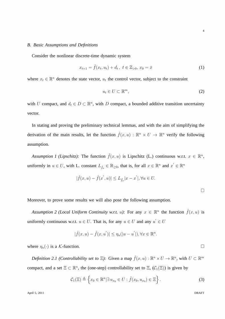
B. Basic Assumptions and Definitions

Consider the nonlinear discrete-time dynamic system

xt+1 = f(xt, ut) + dt , t ∈ Z>0, x0 = x (1)

wherext ∈ Rn denotes the state vector,ut the control vector, subject to the constraint

ut ∈ U ⊂ Rm, (2)

with U compact, anddt ∈ D ⊂ Rn, with D compact, a bounded additive transition uncertainty

vector.

In stating and proving the preliminary technical lemmas, and with the aim of simplifying the

derivation of the main results, let the functionf(x, u) : Rn × U → Rn verify the following

assumption.

Assumption 1 (Lipschitz):The function f(x, u) is Lipschitz (L.) continuous w.r.t.x ∈ Rn,

uniformly in u ∈ U , with L. constantLfx∈ R≥0, that is, for allx ∈ R

n andx′ ∈ R

n

|f(x, u)− f(x′

, u)| ≤ Lfx|x− x

′ |, ∀u ∈ U.

�

Moreover, to prove some results we will also pose the following assumption.

Assumption 2 (Local Uniform Continuity w.r.t.u): For any x ∈ Rn the function f(x, u) is

uniformly continuous w.r.t.u ∈ U . That is, for anyu ∈ U and anyu′ ∈ U

|f(x, u)− f(x, u′

)| ≤ ηu(|u− u′|), ∀x ∈ R

n.

whereηu(·) is aK-function. �

Definition 2.1 (Controllability set toΞ): Given a mapf(x, u) : Rn×U → Rn, with U ⊂ R

m

compact, and a setΞ ⊂ Rn, the (one-step) controllability set toΞ, (C1(Ξ)) is given by

C1(Ξ) ,{

x0 ∈ Rn|∃ ux0 ∈ U : f(x0, ux0) ∈ Ξ

}

. (3)

April 5, 2011 DRAFT

5

�

Definition 2.2 (Predecessor set ofΞ): Given the mapg(x) : Rn → Rn and a setΞ ⊂ R

n, the

(one-step) predecessor ofΞ, (P1(Ξ)) is given by

P1(Ξ) , {x0 ∈ Rn|g(x0) ∈ Ξ} . (4)

�

Definition 2.3 (i-steps Controllability Set toΞ): Given a mapf(x, u) : Rn × U → Rn, with

U ⊂ Rm compact, and a setΞ ⊂ R

n, the i-steps controllability set toΞ, (Ci(Ξ)) is given by

Ci(Ξ) ,{

x0 ∈ Rn|∃ux0 ∈ U i : x(i, x,ux0) ∈ Ξ

}

. (5)

that is,Ci(Ξ) is the set o initial statesx0 ∈ Rn from whichΞ can be reached in exacti steps.�

Definition 2.4 (i-steps Predecessor ofΞ): Given a mapg(x) : Rn → Rn and a setΞ ⊂ R

n,

the i-steps predecessor ofΞ, (Pi(Ξ)) is given by

Pi(Ξ) ,{

x0 ∈ Rn|gi(x0) ∈ Ξ

}

. (6)

�

Definition 2.5 (i-steps Capture Basin toΞ): Given a mapf(x, u) : Rn ×U → Rn, with U ⊂

Rm compact, and a setΞ ⊂ R

n, the i-steps capture basin toΞ, (Capti(Ξ)) is given by

Capti(Ξ) ,i⋃

j=1

Ci(Ξ). (7)

that is,Capti(Ξ) is the set o initial statesx0 ∈ Rn such thatΞ is reached in at mosti steps (i.e.,

∃ux0 ∈ U j : x(j, x0,ux0) ∈ Ξ for at least onej ∈ [1, . . . , i− 1], before possibly leavingΞ. �

Moreover, the following property holds for controllability sets.

Proposition 2.1:Given two setsΞ1 ⊂ Rn andΞ2 ⊂ R

n, thenC1(Ξ1 ∪Ξ2) = C1(Ξ1)∪C1(Ξ2).

�

Proof: From Definition 2.1 we have that

April 5, 2011 DRAFT

6

C1(Ξ1 ∪ Ξ2) , {x ∈ Rn| ∃ux : f(x, ux) ∈ (Ξ1 ∪ Ξ2)}

= {ξ ∈ Rn| ∃uξ : f(ξ, uξ) ∈ (Ξ1)}

∪{x ∈ Rn| ∃ux : f(x, ux) ∈ (Ξ2)}

= C1(Ξ1) ∪ C1(Ξ2),

thus proving the statement.

Definition 2.6 (RC,d1-RC): A compact setΞ⊂Rn is Robustly Controllable (RC) under the

map f(x, u), with u ∈ U , if Ξ ⊆ C1 (int(Ξ)).

A compact setΞ⊂Rn is Robustly Controllable in one-step w.r.t. additive perturbationsd∈

Bn(d1) (d1-RC) if (Ξ∽Bn (d1)) is not empty andΞ⊆C1(Ξ∽Bn (d1)). �

Definition 2.7 (RPI): A compact setΞ⊂ Rn is Robust Positively Invariant (RPI) under the

map g(x), if Ξ ⊆ P1 (int(Ξ)). �

Definition 2.8 (quasi-RPI):A compact setΞ⊂Rn is quasi-Robust Positively Invariant (RPI)

under the mapg(x) with maximum return-timeN , if Ξ ⊆N⋃

i=1

Pi (int(Ξ)) for some finiteN ∈

Z>0; that is, for anyx0 ∈N⋃

i=1

Pi (int(Ξ)) , ∃i ∈ {1, . . . , N} : gi(x0) ∈ int(Ξ). �

Next, some results concerning the properties of robustly controllable sets under Lipschitz maps

are given. These intermediate results will be used in Section IV to prove the main contribution

of the present work.

C. Preliminary Technical Results

In stating and deriving the following technical lemmas, letthe nominal system’s transition

map f verify Assumption 1.

Lemma 2.1 (Technical):Given two compact setsΞ1 ⊂ Rn, Ξ2 ⊂ R

n and a positive scalar

d ∈ R>0, if the following three conditions hold together:i) Ξ1 ⊆ C1(Ξ2), ii) Ξ2 ⊂ Ξ1 and iii)

dist(Rn\Ξ1,Ξ2) ≥ d, thenΞ1 is d-RC. �

April 5, 2011 DRAFT

7

Proof: The two conditionsii) and iii) together imply that

Ξ2 ⊆ Ξ1 ∽Bn(d). (8)

Finally, from the inclusionΞ1 ⊆ C1(Ξ2) and (8) it follows that

Ξ1 ⊆ C1(

Ξ1 ∽Bn(d))

,

which proves the statement of the Lemma.

Lemma 2.2 (Technical):Given a compact setΞ ⊂ Rn, assume thatC1(Ξ) is non-empty. Then,

for any arbitraryη ∈ R≥0 it holds that:

∀x ∈ Ξ⊕ Bn(

L−1

fxη)

, ∃ ux ∈ U : f(x, ux) ∈ Ξ⊕ Bn(η). (9)

�

Proof: Consider the setC1(Ξ)⊕ B(L−1

fxη). It holds that∀x∈

(

C1(Ξ)⊕ B(Lf−1xη))

, ∃ ξx ∈

C1(Ξ) such that

|x− ξx| ≤ L−1

fxη. (10)

The inclusionξx ∈ C1(Ξ) implies that∃ uξx ∈ U : f(ξx, uξx) ∈ Ξ. Since f is Lipschitz, then

|f(x, uξx)− f(ξx, uξx)| ≤ Lfx|x− ξx|. From (10), it follows that

|f(x, uξx)− f(ξx, uξx)| ≤ η. (11)

which finally yields to the statement of the Lemma.

.

Lemma 2.3 (Technical):Given a compact setΞ ⊂ Rn and positive scalarρ ∈ R>0, if Ξ is

ρ-RC, thenC1(Ξ) is (L−1

fxρ)-RC. �

Proof: Consider the setΞ ⊕ B(L−1

fxρ). It holds that∀ξ ∈ (Ξ ⊕ B(L−1

fxρ)), ∃xξ ∈ Ξ and

∃uxξ∈U such that|ξ−xξ| ≤L−1

fxρ and f(xξ, uxξ

)∈ (Ξ∽Bn(ρ)). Let us poseuξ = uxξ. Then,

in view of Assumption 1, it holds thatf(ξ, uξ) ∈ Ξ, ∀ξ ∈ (Ξ ⊕ B(L−1

fxρ)), which implies that

April 5, 2011 DRAFT

8

C1(Ξ)⊇ (Ξ ⊕ B(L−1

fxρ)) and thatdist(Rn\C1(Ξ),Ξ)≥L−1

fxρ. Finally, thanks to Lemma 2.1, the

statement follows.

.

The following technical result will establish the invariant properties of theN-steps control-

lability set CN (Ξ) of a givenρ-RC setΞ. Moreover, an inner (conservative) approximation of

CN (Ξ), containingΞ in its interior, will be provided.

Lemma 2.4 (Technical):Given a compact setΞ ⊂ Rn, a finite integerN ∈ Z>0 and a positive

scalarρ ∈ R>0, if Ξ is ρ-RC, then

i) CN(Ξ) is (L−N

fxρ)-RC.

ii) CN (Ξ) ⊇ Ξ⊕ Bn

(

1− L−N

fx

Lfx− 1

ρ

)

�

Proof: Applying recursively Lemma 2.3, it holds that

dist(Rn\Ci(Ξ), Ci−1(Ξ)) ≥ L−i

fxρ, ∀i ∈ Z>0, (12)

with C0(Ξ) = Ξ. Therefore we obtain

dist(Rn\CN(Ξ),Ξ) ≥ ρN∑

i=1

L−i

fx=

1− L−N

fx

Lfx− 1

ρ. (13)

Finally, the statement follows from inequality (13) and Lemma 2.1.

The following important result, that will play a key role in characterizing the robust stability

properties of nonlinear minimum-time control laws, can nowbe proven. The reader can refer

to Figure 1 for a schematization of the sets involved in the statement and in the proof of the

forthcoming theorem.

Theorem 2.1 (N-steps Reachability Implication):Given a compact setΞ ⊂ Rn and map

f(x, u) verifying Assumption 1 and subject to (2), if the following inclusion holds for a finite

integerN ∈ Z>0 and for a positive scalarρN ∈R>0:

Ξ⊆CaptN (Ξ)∽Bn(ρN), (14)

April 5, 2011 DRAFT

9

Ξ

C1(Ξ)

C2(Ξ)

Ci(Ξ)

CN (Ξ)

∂ CaptN(Ξ)

∂ CaptN(Ξ, dN )

Fig. 1. Scheme of the sets involved in the statement and proofof Theorem 2.1.CaptN (Ξ) denotes theN -steps capture basin

of Ξ, while CaptN (Ξ, dN ) is an extension of the nominal capture basin (see (15)) that can be proven to be robust positively

controllable. That is, there exists a control law, compliant with the input constraints, that rendersCaptN(Ξ, dN ) RPI.

(i.e.,Ξ is reachable in at mostN steps from a set containingΞ in its interior under the nominal

map f(x, u)), then the set

CaptN (Ξ, dN) , CN (Ξ) ∪(

N−2⋃

i=1

[

Ci+1(Ξ)⊕ B(

L−1

fxηi

)]

)

∪(

C1(Ξ)⊕ B(

L−1

fxη0

))

(15)

is dN -RC, with ηi positive scalars depending ondN according to the recursion

dN,Lfx−1

LN

fx−1

ρN ,

η0 = ρN − dN ,

(16)

and

ηi = L−1

fxηi−1 − dN , ∀i ∈ {1, . . .N − 2}.

�

Proof: Assume, at this stage, that the condition (14) holds forN = 1. In this case the set

Capt1(Ξ, d1) = C1(Ξ) is d1-RC by definition, withd1 = ρ1.

Now, let us considerN=2 and ρ2 = dist(Rn\C2(Ξ),Ξ). BeingΞ⊆ (Capt2(Ξ)∽Bn(ρ2)), it

follows that,

April 5, 2011 DRAFT

10

∀x∈C1(Ξ), ∃ ux∈U : f(x, ux)∈(Capt2(Ξ)∽Bn(ρ2)), (17)

which, in view of Lemma 2.2, implies that

∀x∈C1(Ξ)⊕ B(

L−1

fxη0

)

, ∃ ux∈U : f(x, ux)∈(Capt2(Ξ)∽Bn(ρ2 − η0)) , (18)

for all η0 ∈ [0, ρ2] . Moreover, from the definition ofC2(Ξ), we recall that

∀x∈C2(Ξ), ∃ ux∈U : f(x, ux)∈C1(Ξ), (19)

Now, from (18),(19) and Property 2.1 it follows that

∀x∈C2(Ξ) ∪[

C1(Ξ)⊕ Bn(

L−1

fxη0

)]

, ∃ ux∈U : f(x, ux)∈C1(Ξ) ∪ [Capt2(Ξ)∽Bn(ρ2 − η0)] ,

(20)

that is

C2(Ξ) ∪[

C1(Ξ)⊕ Bn(

L−1

fxη0

)]

⊆ C1(

C1(Ξ) ∪ [Capt2(Ξ)∽Bn(ρ2 − η0)])

, (21)

Moreover, ifη0 ∈ (0, ρ2), then it holds that

C1(Ξ) ∪ [Capt2(Ξ)∽Bn(ρ2 − η0)] ⊂ C2(Ξ) ∪[

C1(Ξ)⊕ Bn(

L−1

fxη0

)]

(22)

Finally, from the topology of the sets involved in the underlying analysis it follows that

dist(

Rn\(

C2(Ξ) ∪[

C1 ⊕ Bn(

L−1

fxη0

)])

, C1(Ξ) ∪ [Capt2(Ξ)∽Bn(ρ2 − η0)])

≥ min{

L−1

fxη0, ρ2 − η0

}

.

(23)

Now, consider the caseρ2 − η0 = L−1

fxη0. Posing

η0 ,(

1 + L−1

fx

)−1

ρ2 =Lfx

Lfx+ 1

ρ2

then inequality (23) holds with positive right-hand side:

dist(

Rn\(

C2(Ξ) ∪[

C1 ⊕ Bn(

L−1

fxη0

)])

, C1(Ξ) ∪ [Capt2(Ξ)∽Bn(ρ2 − η0)])

≥ ρ2−η0 =1

1 + Lfx

ρ2.

(24)

April 5, 2011 DRAFT

11

In view of Lemma 2.1, (21), (22) and (24) together imply that the setCapt2(Ξ, d2) = C2(Ξ) ∪[

C1 ⊕ Bn(

L−1

fxη0

)]

is d2-RC, with

d2 =1

1 + Lfx

ρ2.

Now let us consider the caseN = 3 and ρ3 = dist (Rn\Capt3(Ξ), Xi). Being Ξ ⊆

(Capt3(Ξ) ∽Bn(δ3)), it follows that

∀x∈C1(Ξ), ∃ ux∈U : f(x, ux)∈(Capt3(Ξ)∽Bn(ρ3)), (25)

which, in view of Lemma 2.2, implies that

∀x∈C1(Ξ)⊕ B(

L−1

fxη0

)

, ∃ ux∈U : f(x, ux)∈(Capt3(Ξ)∽Bn(ρ3 − η0)) , (26)

for all η0 ∈ [0, ρ3]. Moreover, from the definition ofC2(Ξ) (see (19)) and by exploiting Lemma

2.2, we have that

∀x∈C2(Ξ)⊕ B(

L−1

fxη)

, ∃ ux∈U : f(x, ux)∈C1(Ξ)⊕ B (η) , (27)

for all η ∈ R≥0. Finally, from the definition ofC3(Ξ), we have that

∀x∈C3(Ξ), ∃ ux∈U : f(x, ux)∈C2(Ξ), (28)

From (26), (27), (28) and thanks to Property 2.1, then the following inclusion holds

C3(Ξ) ∪(

C2(Ξ)⊕ B(

L−1

fxη))

∪(

C1(Ξ)⊕ B(

L−1

fxη0

))

⊆ C1

(

C2(Ξ) ∪(

C1(Ξ)⊕ B (η))

∪(

Capt3(Ξ)∽Bn(ρ3 − η0))

)

(29)

Moreover, ifη > 0, η < Lfx

−1η0 andη0 ∈ (0, ρ3), then the following inclusion holds

C2(Ξ) ∪(

C1(Ξ)⊕ B (η))

∪(

Capt3(Ξ)∽Bn(ρ3 − η0))

⊂ C3(Ξ) ∪(

C2(Ξ)⊕ B(

L−1

fxη))

∪(

C1(Ξ)⊕ B(

L−1

fxη0

))(30)

Finally, from the topology of the sets involved it turns out that

dist

(

Rn\[

C3(Ξ) ∪(

C2(Ξ)⊕ B(

L−1

fxη))

∪(

C1(Ξ)⊕ B(

L−1

fxη0

))

]

,

[

C2(Ξ) ∪(

C1(Ξ)⊕ B (η))

∪(

Capt3(Ξ)∽Bn(ρ3 − η0))

])

≥ min{

ρ3 − η0, L−1

fxη0 − η, L−1

fxη}

(31)

April 5, 2011 DRAFT

12

Choosingη0 and η such that all the three terms in the right-hand side of (31) are equal, then

inequality (31) holds with positive right-hand side.

Thanks to Lemma 2.1, then (29), (30) and (31) together imply that the setCapt3(Ξ, d3) =

C3(Ξ)∪(

C2(Ξ)⊕ B(

L−1

fxη))

∪(

C1(Ξ)⊕ B(

L−1

fxη0

))

is d3-RC,with d3 = (L2fx+Lfx

+1)−1ρ3.

Now, we seek for a generalization of the three-step analysisabove to the genericN ≥ 3 case.

Let ρN = dist (Rn\CaptN(Ξ),Ξ) > 0. BeingΞ ⊆ (CaptN (Ξ) ∽Bn(δN)), it follows that

∀x∈C1(Ξ), ∃ ux∈U : f(x, ux)∈(CaptN(Ξ)∽Bn(ρN )), (32)

which, in view of Lemma 2.2, implies

∀x∈C1(Ξ)⊕ B(

L−1

fxη0

)

, ∃ ux∈U : f(x, ux)∈(CN (Ξ)∽Bn(ρN − η0)) , (33)

for all η0 ∈ [0, ρN ]. Now, let us consider the setsCi(Ξ) andCi+1(Ξ), with i ∈ {1, . . . , N − 2}.

By exploiting Lemma 2.2, we have that

∀x∈Ci+1(Ξ)⊕ B(

L−1

fxηi

)

, ∃ ux∈U : f(x, ux)∈Ci(Ξ)⊕ B (ηi) , (34)

for all ηi ∈ R≥0. By using, again, Lemma 2.2, we obtain

∀x∈CN (Ξ), ∃ ux∈U : f(x, ux)∈CN−1(Ξ), (35)

From (33), (34), (35), thanks to Property 2.1, it follows that

CN (Ξ) ∪(

N−2⋃

i=1

[

Ci+1(Ξ)⊕ B(

L−1

fxηi

)]

)

∪(

C1(Ξ)⊕ B(

L−1

fxη0

))

⊆ C1

(

CN−1(Ξ) ∪(

N−2⋃

i=1

[Ci(Ξ)⊕ B (ηi)])

∪(

CaptN(Ξ)∽Bn(ρN − η0))

)

.

(36)

Moreover, if η0 ∈ (0, ρN), η1 < Lfx

−1η0 and ηi < Lfx

−1ηi−1, ∀i ∈ {1, . . . , N − 2}, with

ηi ∈ R>0, ∀i ∈ {1, . . . , N − 2}, then the following inclusion holds

CN−1(Ξ) ∪(

N−2⋃

i=1

[Ci(Ξ)⊕ B (ηi)])

∪(

CaptN(Ξ)∽Bn(ρN − η0))

⊂ CN (Ξ) ∪(

N−2⋃

i=1

[

Ci+1(Ξ)⊕ B(

L−1

fxηi

)]

)

∪(

C1(Ξ)⊕ B(

L−1

fxη0

))

.

(37)

April 5, 2011 DRAFT

13

Finally, from the topology of the sets involved it turns out that

dist

(

Rn\[

CN(Ξ) ∪(

N−2⋃

i=1

[

Ci+1(Ξ)⊕ B(

L−1

fxηi

)]

)

∪(

C1(Ξ)⊕ B(

L−1

fxη0

))

]

,

[

CN−1(Ξ) ∪(

N−2⋃

i=1

[Ci(Ξ)⊕ B (ηi)])

∪(

CaptN(Ξ)∽Bn(ρN − η0))

])

≥ min{

ρN − η0, L−1

fxη0 − η1, . . . , L

−1

fxηi−1 − ηi, . . . , L

−1

fxηN−3 − ηN−2, L

−1

fxηN−2

}

(38)

Choosingη0 andηi, i ∈ {1, . . . , N − 2} such that all theN terms in the right-hand side of (38)

are equal, then inequality (38) holds with positive right-hand side.

Hence, in view of Lemma 2.1, (36), (37) and (38) together imply that the set (extendedN-steps

capture basin)

CaptN (Ξ, dN) , CN (Ξ) ∪(

N−2⋃

i=1

[

Ci+1(Ξ)⊕ B(

L−1

fxηi

)]

)

∪(

C1(Ξ)⊕ B(

L−1

fxη0

))

(39)

is dN -RC, with

dN =

(

N−1∑

i=0

Li

fx

)−1

ρN =Lfx− 1

LN

fx− 1

ρN (40)

Remark 2.1:Note that, if the target setΞ is not ρ-RC, then the region( CaptN(Ξ)\CN (Ξ) )

may even be not empty. In this case, for any initial conditionin ( CaptN (Ξ)\CN(Ξ) ), the state

cannot be driven toΞ in exactN steps, butΞ can be reached for somei with i < N from the

capture basin. Therefore, condition (14) (reachability inat mostN steps) is less restrictive than

requiring the exactN-steps controllability ofΞ. �

III. PROBLEM STATEMENT

The minimum-time problem for discrete-time system not affected by uncertainties has the

following well known formulation: given an initial statex0 ∈ Rn and a target setΞ ⊂ R

n,

find a sequence of control actionsu ∈ MU which minimizes the timeTMT (x0|Ξ) such that

x(x0, TMT ,u) ∈ Ξ. In the following we will denote asT oMT (x0|Ξ) the minimum reach time.

April 5, 2011 DRAFT

14

The above formulation is commonly referred to as the open-loop approach to the minimum-

time problem, that is, an optimal control sequence is determined on the basis of the particular

initial state, relying on a nominal model of the controlled system. In the linear framework, it is

well-known that the minimum-time problem admits a feedbacksolution, that is, it is possible to

determine a control functionu = κMT (x|Ξ) such thatTMT (·|Ξ) is minimized for any possible

initial state. We point out the minimum-time control lawκMT (·|Ξ) is not, in general, unique.

Therefore, for the sake of the present discussion, the notation κMT (x|Ξ) will denote an arbitrary

selection among the possible minimum-time feedback laws.

In nominal conditions, open-loop and feedback formulations are equivalent in the sense that

a feedback solution is optimal if and only if for any initial statesx0 the control sequenceu

produced by the controlu = κMT (x,Ξ) along the systems’trajectory is optimal in the open-

loop sense. On the other side, the feedback approach allows also to embed in the design of the

controller some a priori information on the disturbances/uncertainties, yielding to minimum-time

control laws with enhanced robustness properties. However, for a generic nonlinear system, it

is very difficult to obtain an explicit minimum-time controlfunction, even in the nominal case.

Moreover, in practice, the search for a minimum-time open-loop sequence is performed over a

compact set of sequences of finite length, subsuming a specified upper boundN ∈ Z>0.

A viable solution to alleviate the lack of robustness of open-loop approaches consists in

solving, along system trajectories, a finite-time optimization problem in a receding horizon

(RH) fashion. In the sequel, we will determine sufficient conditions (related, in particular, the

controllability and reachability properties of the targetset) under which the RH implementation

guarantees the recursive feasibility of the optimization (that is, the robust postive invariance or

the quasi-invariance of the feasible region) and the boundedness of the closed-loop trajectories.

Problem 3.1 (RH Nominal Minimum-Time Control):Given a compact admissible setU ⊂ Rm

for the input of the system (1), a compact target setΞ ⊂ Rn, a finite integerN ∈ Z>0 and the

April 5, 2011 DRAFT

15

nominal state-transition mapf(x, u) of the system, at each timet ∈ Z≥0 determine a sequence

uo[t,t+N−1] = {uo

t , uot+1, . . . , u

ot+N−1}, in correspondence of the current state measurementxt, such

that:

TNMT (xt,uo[t,t+N−1]|Ξ, N) = T o

MT (xt|Ξ),

with

TNMT (xt,u[t,t+N−1]|Ξ, N) , min{

τ ∈ {1, . . . , N} : x(τ, xt,u[t,t+τ−1]) ∈ Ξ}

, (41)

and

T oMT (xt|Ξ) , min

u[t,t+N−1]∈UN

{

TNMT (xt,u[t,t+N−1]|Ξ, N)}

,

then apply to the plant the first element ofuo[t,t+N−1] by settingut = uo

t . �

If the Problem 3.1 is feasible inxt, thenuot is a selection among the admissible minimum-time

control actions for the current state, i.e.,uot ∈ KMT (xt|Ξ).

This problem can be solved, in the discrete-time framework,by checking the feasibility of

the target set constraint in (41). The feasibility check approach consists in embedding Problem

3.1 into a family of input-constrained minimum-distance problems as follows:

JoMD(xt|Ξ, τ) = min

u[t,t+τ−1]∈UτΦ(

x(τ, xt,u[t,t+τ−1]),Ξ)

. (42)

parametrized by the integerτ ∈ Z>0. For a givenτ , the minimizer is a fixed-length sequence

ut,t+τ−1 belonging to the compact setU τ .

The feasible region for the original problem 3.1 is the basinof captureCaptN (Ξ), which

verifies

CaptN (Ξ) = {xt ∈ Rn ∃ τ ∈ {1, . . . , N} : Jo

MD(xt,Ξ, τ) ≤ 0} .

Then, assuming thatxt ∈ CaptN (Ξ), at each timet ≥ 0 the optimal timeT oMT (xt|Ξ) is

determined as the minimum amongτ ∈ {1, . . . , N} for which problem (42) yields to

JoMD(xt|Ξ, τ) ≤ 0, (43)

April 5, 2011 DRAFT

16

that is

T oMT (xt|Ξ) = min {τ : Jo

MD(xt|Ξ, τ) ≤ 0}

The conditionJoMD(xt|Ξ, τ) ≤ 0 represents a feasibility test aimed to ensure thatxt belongs to

the τ -steps capture basin ofΞ.

Once the minimum-timeT oMT (xt|Ξ) has been determined, we can take as a solution any control

sequence which may steer the state toΞ in T oMT (xt|Ξ) steps. A simple choice is

uo[t,t+T o

MT(xt|Ξ)−1] = arg min

u[t,t+ToMT

(xt|Ξ)−1]∈UToMT

(xt|Ξ)JoMD

(

xt Ξ, T oMT (xt|Ξ)

)

(44)

It is important to determine those conditions under which, starting fromx0 ∈ CaptN(Ξ), the

trajectories remain in the feasible set, in order to guarantee the solvability of the optimization

at each timet > 0.

IV. RECURSIVE FEASIBILITY UNDER THE NOMINAL NONLINEAR

MINIMUM-TIME CONTROL WITH ROBUST POSITIVELY CONTROLLABLE

TARGET SET

In case the target setΞ is robust positively controllable (i.e., there exists an admissible control

law which rendersΞ RPI), then theN−steps basin of captureCaptN (Ξ) coincides with the

N-steps controllability set ofΞ. MoreoverCaptN(Ξ) is RPI under the minimum-time control,

as formally stated by the following theorem.

Theorem 4.1 (Ξ ρ-RC→ CaptN(Ξ) RPI): Given aρ−RC compact target setΞ ⊂ Rn, then

the Nominal nonlinear Minimum-Time ControlκMT (xt) guarantees the boundedness of the

closed-loop trajectories within the setCaptN (Ξ), for any initial conditionx0 ∈ CaptN(Ξ) and

for any admissible uncertainty realizationd ∈MBn(dN ), with dN = L−N

fxρN .

Moreover, the closed-loop trajectories starting at timet = 0 from any pointx(0) = x0 ∈

CaptN (Ξ) are ultimately bounded in the compact set

ΥN (Ξ, dN) , Ξ⊕ B(

LN

fx− 1

Lfx− 1

dN

)

⊆ CaptN (Ξ), (45)

April 5, 2011 DRAFT

17

which is reached in finite time, for any possible realizationof the uncertainties (d ∈MBn(dN )),

that is,x(t, x0,u[0,t−1],d[0,t−1]) ∈ ΥN (Ξ, ||d[0,t−1]||) ⊆ ΥN(Ξ, dN), ∀x0 ∈ CaptN(Ξ), ∀t ≥ N ,

∀d[0,t−1] : ||d[0,t−1]|| ≤ dN . �

Proof: First, the boundedness of the trajectories can be proven by showing thatCaptN(Ξ)

is RPI under the minimum-time control for anyd ∈MBn(dN ).

Indeed, applying recursively Theorem 2.3, it holds that

Ci(Ξ) ⊃ Ci−1(Ξ), ∀ i > 1,

which yields to

CN (Ξ) ⊃ Cj(Ξ), ∀ j ∈ {1, . . . , N − 1},

that finally implies

CN (Ξ) ≡ CaptN(Ξ). (46)

Moreover, thanks to Pointi) of Lemma 2.4, it holds thatCN−1(Ξ) ∈ CN (Ξ) ∽Bn(L−N

fxρ),

which, thanks to (46), implies that∀x ∈ CaptN(Ξ), u = κMT (x) : f(x, u) + d ∈ CaptN(Ξ),

∀d ∈ Bn(L−N

fxρ) (that is,CaptN(Ξ) is RPI underκMT (x)).

Now, we will prove the ultimate boundedness of the trajectories in the setΥN(Ξ, dN). Let

us consider the optimal minimum-time sequenceuo[0,N−1], computed in open-loop at timet = 0

for the initial conditionx0 ∈ Capt(Ξ), and the correspondent nominal finite-time trajectory

x(i, x0,uo[0,i−1]), ∀i ∈ {1, . . . , N}. The true evolution of the perturbed system, driven byu

o[0,N−1],

can be bounded by

|x(i, x0,uo[0,i−1])− x(t, x0,u

o[0,i−1],d[0,i−1])| ≤

Li

fx− 1

Lfx− 1||d[0,i−1]||, ∀i ∈ {1, . . . , N} (47)

for any admissible realization of the uncertaintiesd[0,i−1]. In particular, sincex(N, x0,uo[0,N−1]) ∈

Ξ, we have that

x(N, x0,uo[0,N−1],d[0,N−1]) ∈ Ξ⊕ Bn

(

LN

fx− 1

Lfx− 1||d[0,N−1]||

)

⊆ ΥN(Ξ, dN). (48)

April 5, 2011 DRAFT

18

If, in addition, ||d|| ≤ L−N

fxρ, then the closed-loop trajectories remain in the feasible set (in

particular,x1 ∈ Capt(Ξ)). At time t = 1, the minimum-time control problem inx1 can be

solved with respect to a new open-loop sequence of controlsuo[1,N ]. Proceeding along the same

lines as above, it is possible to bound the finite-time perturbed evolution of the system as follows

x(N + 1, x1,uo[1,N ],d[1,N ]) ∈ Ξ⊕ Bn

(

LN

fx− 1

Lfx− 1||d[1,N ]||

)

⊆ ΥN(Ξ, dN). (49)

Moreover,x2 ∈ Capt(Ξ) for any possible uncertainty realization. By induction, itfollows that

the closed loop trajectories remain bounded inΥN (Ξ, dN) for any t ≥ N .

Now, our analysis will be extended to the case in whichΞ is not one step robust positively

controllable. In this regard, the result of Theorem 2.1, obtained by set-invariance theoretic

analysis, implies the existence of a (possibly non unique) control law which renders the set

CaptN (Ξ, dN) a dN -RPI set, withdN defined in (16). However, for non null-uncertainties, the

setCaptN(Ξ, dN) is such thatCaptN (Ξ, dN) ⊃ CaptN (Ξ). Recalling the the feasible region for

Problem 3.1 is as small asCaptN(Ξ), in the setCaptN(Ξ, dN)\CaptN(Ξ) the finite-time RH

problem does not admit a solution (i.e., the feasibility check (43) fails). Therefore, we seek for

a backup control law to be applied inCaptN(Ξ, dN) when the minimum-time problem is not

solvable, but capable to keep the trajectories bounded in the extendedN-steps capture basin

CaptN (Ξ, dN). Notably, by Theorem 2.1 we have established the existence of a control law,

compliant with the input constraints, capable to achieve this task. We are now on the way to

show how such a robust control law can be obtained.

V. ROBUST NONLINEAR MINIMUM-TIME CONTROL LAWS WITH NON ROBUST

POSITIVELY CONTROLLABLE TARGET SETS

In the following, we are going to describe a modified minimum-time control scheme, which

will be referred to as Robustified Nonlinear Minimum-Time Control (RNMT), that guarantees the

quasi-invariance of the feasible region, despite bounded uncertainties and with mild assumptions

April 5, 2011 DRAFT

19

on the target setΞ. The RNMT control, computed online according to Procedure 5.1 below,

consists in a control schemes that switches between the regular minimum-time control and

a backup control action when transitory unfeasibility occurs; hence, in nominal conditions, the

RNMT corresponds to the convential receding horizon minimum-time control, being the feasible

region invariant in this case. Conversley, in perturbed conditions, the backup control action is

taken from a buffer in which a time-optimal control sequencehad been saved after the most

recent feasible optimization. The key point of this procedure is that feasbility is recovered before

buffer overrun occurs. As long as the system’s state enters the feasible region, an optimal solution

is computed and the buffer is reinitialized with a new sequence, that will be used to cope with

future infeasibility occurences.

Next, the RNMT scheme is formalized by a listed procedure describing the actions to be

performed by the controller.

Procedure 5.1 (RNMT):Let the controller be equipped with two buffers:i) ub ∈ R

m × N ,

used to store a sequence ofN control actions;ii) T b ∈ Z, that stores the time instant in which

the sequence stored inub had been computed. Moreover, let us denote as← a data assignment

operation. Given the buffer (memory array)ub, let ub(i) represent thei-th element of the array,

with i ∈ {1, . . . , N}.

Initialization

1 Assuming that, at time instantt = 0, the initial condition verifiesx0 ∈ CaptN(Ξ), solve the

nominal minimum-time Problem 3.1 obtaining an optimal control sequenceuo0,N−1;

2 storeub ← uo0,N−1;

3 storeT b ← 0;

4 applyuo = ub(1) to the plant.

On-line Control Computation

1 for t ∈ Z>0 :

April 5, 2011 DRAFT

20

2 givenxt, perform the feasibility test (43) forτ ∈ {1, . . . , N};

3 if exists at least oneτ for which JoMD(xt|Ξ, τ) ≤ 0, then :

4 computeuot,t+N−1 with (44) ;

5 overwrite the bufferub ← uot,t+N−1;

6 setT b ← t;

7 end if;

8 applyut = ub(t− T b + 1) to the plant;

9 end for;

�

The following theorem formally states the recursive feasibility property (that is, the quasi-

invariance of the feasible region) of the RNMT scheme for bounded additive uncertainties.

Theorem 5.1 (Quasi-invariance of the feasible set):Given a compact target setΞ ⊂ Rn

(possibly not robustly controllable) such thatΞ ⊆ CaptN(Ξ) ∽Bn(ρN), then, for any initial

condition x0 ∈ CaptN(Ξ), the RNMT controlut = κRNMT (t, xt) guarantees that the closed-

loop system’s trajectory is ultimately contained inCaptN(Ξ, dN) for any admissible uncertainty

realizationd ∈ MBn(dN ), with dN given by (16). Moreover, the compact setΥN(Ξ, dN ) ⊆

CaptN (Ξ) (defined in (51) below) is reached in finite-time fromx0 and is quasi-RPI in closed-

loop, for any possible realization of the uncertainties. �

Proof: The quasi-invariance result can be obtained by induction: given x0 ∈ CaptN(Ξ),

the optimal minimum-time sequenceuo[0,T o

MT(x0)−1] computed at timet = 0 yields to

x(T oMT (x0), x0,u

o[0,T o

MT(x0)−1]) ∈ Ξ for the nominal trajectory. Now, the true trajectory departing

April 5, 2011 DRAFT

21

from x0 is bounded in a closed envelope around the nominal one, for all t ∈ {1, . . . , T oMT (x0)}

∣

∣

∣x(t, x0,u

o[0,t−1],d[0,t−1])− x(t, x0,u

o[0,t−1])

∣

∣

∣

≤Lt

fx− 1

Lfx− 1

(

ηu(u) + ||d[0,t−1]||)

,

≤Lt

fx− 1

Lfx− 1

dN ,

(50)

for any bounded sequenced[0,T oMT

(x0)−1] ∈(

Bn(dN))T o

MT(x0). At time t = T o

MT (x0) we have∣

∣

∣x(T o

MT (x0), x0,uo[0,T o

MT(x0)−1],d[0,T o

MT(x0)−1])− x(T o

MT (x0), x0,uo[0,T o

MT(x0)−1])

∣

∣

∣

≤LT oMT

(x0)

fx− 1

Lfx− 1

dN .

Now, defining the set

ΥN(Ξ, dN) , Ξ⊕ Bn

(

maxj∈{1,...,N}

{

Lj

fx− 1

Lfx− 1

dN

})

(51)

it holds that

xT o0= x

(

T oMT (x0), x0,u

o[0,T o

MT(x0)−1]

)

∈ ΥN(Ξ, dN) ⊆ CaptN(Ξ) (52)

under the closed-loop RNMT control. In view of the inclusion(52) , at time T o0 =

T oMT (x0) a feasible time-optimal sequence can be computed, and the same arguments can

be used to show that the perturbed closed-loop trajectory departing from xT o0

verifies

x(

T oMT (xT o

0), xT o

0,u[T o

0 ,ToMT

(xTo0))−1]

)

∈ ΥN(Ξ, dN).

Therefore, the return-time toCaptN (Ξ) from a pointx0 with minimum-timeT o0 = T o

MT (x0)

never exceedes the minimum-time itself. This key result establishes the inherent buffer-underrun

consistency of the RNMT scheme. Proceeding by induction, itfollows that the compact set

ΥN(Ξ, dN ) ⊆ CaptN(Ξ) and the feasible setCaptN(Ξ) are both quasi-RPI (see Definition 2.8)

under the closed-loop trajectories with maximum return-timeN .

Now, we will prove that the trajectories are confined inCaptN (Ξ, dN) during the transitory

departures fromCaptN (Ξ) . The setCaptN(Ξ, dN), defined in (15), can be equivalently expressed

April 5, 2011 DRAFT

22

as

CaptN(Ξ, dN) = CN (Ξ) ∪(

N−2⋃

i=1

[Ci+1(Ξ)⊕ B (ǫi+1)]

)

∪ (C1(Ξ)⊕ B (ǫ1)) (53)

where

ǫi , L−1

fxηi−1 =

LN−i

fx− 1

Lfx− 1

dN ,

for all i ∈ {1, . . . , N − 1}. Since by (50) it holds that

∣

∣

∣x(i, x0,u

o[0,t−1],d[0,t−1])− x(t, x0,u

o[0,t−1])

∣

∣

∣≤ ǫN−i, (54)

for all i ∈ {1, . . . , N − 1}, and andx(i, x0,uo[0,t−1] ∈ CN−i), ∀i ∈ {1, . . . , N − 1} then we can

conlude that

x(i, x0,uo[0,t−1],d[0,t−1]) ∈ CN−i(Ξ)⊕ B (ǫN−i) ⊆ CaptN(Ξ, dN), ∀i ∈ {1, . . . , N − 1}. (55)

Proceeding by induction, it follows that the closed-loop trajectories are ultimately confined in

CaptN (Ξ, dN).

Notice that the ultimate confinement property inCaptN(Ξ, dN), together with the quasi-robust

positive invariance of the compact setΥN(Ξ, dN), they by themselves do not imply the ultimate

boundedness of the trajectories, sinceCaptN(Ξ, dN) can be unbounded. The boundedness in a

compact subset ofCaptN(Ξ, dN) can be proven by invoking the further Assumption 2 and by

exploiting the the presence of input contraints.

Corollary 5.1 (Ultimate boundedness):If the nominal transition function of the system,f ,

verifies, in addition to Assumptions of Theorem 5.1, the further Assumption 2, (d ∈MBn(dN )),

then the closed-loop trajectories under the RNMT control are ultimately bounded in a compact

set ΛN(Ξ, dN , u) (defined in (56) below) for any initial conditionx0 ∈ CaptN(Ξ), that

is: x(t, x0,u[0,t−1],d[0,t−1]) ∈ ΛN(Ξ, dN , u), ∀x0 ∈ CaptN(Ξ, dN), ∀t ≥ N , ∀d[0,t−1] :

||d[0,t−1]|| ≤ dN . �

April 5, 2011 DRAFT

23

Proof: First, note that the setΥN(Ξ, dN) is reached in finite-time (in at mostN steps).

Hence, for somek ∈ {1, . . . , N} we have thatxk ∈ ΥN(Ξ, dN). Moreover, by the quasi-

invariance property, the trajectories departing fromxk are guaranteed to enter again inΥN(Ξ, dN)

in at most furtherN steps. Let us analyze the closed-loop perturbed trajectoryxk+j for the worst-

case-length interval in which the trajectories may live outsideΥN(Ξ, dN ). We have that, for any

j ∈ {1, . . . , N},

|x(k + j, xk,u[k,k+j−1],d[k,k+j−1])| ≤ Lj

fx|xk|+

Lj

fx− 1

Lfx− 1

(

ηu(||u[k,k+j−1]||) + ||d[k,k+j−1]||)

≤ Lj

fx|xk|+

Lj

fx− 1

Lfx− 1

(

ηu(u) + d)

.

whereu , maxu∈U{|u|} Therefore, for anyj ∈ {1, . . . , N}, the trajectories remain bounded in

ΛN(Ξ, dN , u) , CaptN(Ξ) ∩ ΥN(Ξ, dN , u)⊕Bn

(

maxj∈{1,...,N}

{

Lj

fx− 1

Lfx− 1

(

ηu(u) + dN)

})

. (56)

The ultimate boundedness of the closed-loop trajectories follows from the compactness of

ΛN(Ξ, dN , u).

VI. A CADEMIC EXAMPLE

To show the effectiveness of the method, we will apply the robustified nonlinear minimum-time

control to the following discrete-time open-loop unstablesystem:

x(1)t+1= x(1)t

[

1.1 + 0.4 sign(x(1)t)ut

]

+ (x(2)2t+ 2)−1ut + d(1)t

x(2)t+1= 0.94 x(2)t

− x(2)tut + d(2)t

, t ∈ Z≥0. (57)

subjected to the input constraint|ut| < 2. The subscripts(i), i ∈ {1, 2} in (57) denote thei-th

component ofxt ∈ R2, while dt ∈ R

2 is a bounded exogenous disturbance. First, we will prove

that the nominal transition function of the system is Lipschitz continuous with respect to the

state variables.

April 5, 2011 DRAFT

24

Proposition 6.1:The nonlinear transition functionf(x, u) : R2 × [−R,R] → R

2, with

f(x, u) =(

f(1)(x(1), x(2), u), f(2)(x(2), u))

given by

f(1)(x(1), u) = x(1)

[

1.1 + 0.4 sign(x(1))u]

+ (x(2)2 + 2)−1u,

f(2)(x(2), u) = 0.94 x(2) − x(2) u,(58)

is Lipschitz continuous inx, uniformly for u ∈ [−2, 2].

Proof: Consider the scalar functionf(1)(x(1), x(2), u) : R2 × [−2, 2]→ R. Then, given two

points(x(1), x(2)) and (x′

(1), x′

(2)) = (x(1) + δx(1), x(2) + δx(2)), for any fixedu we have

∣

∣

∣f(1)(x

′

(1), x(2)′, u)− f(1)(x(1), x(2)t

, u)∣

∣

∣

≤∣

∣

∣(x(1) + δx(1))

[

1.1 + 0.4 sign(x(1) + δx(1))u]

+1

(x(2) + δx(2))2 + 2u

−x(1)

(

1.1 + 0.4 sign(x(1))u)

+1

x(1)2 + 2

u∣

∣

∣

≤∣

∣

∣(x(1) + δx(1))

(

1.1 + 0.4 sign(x(1) + δx(1))u)

− x(1)

(

1.1 + 0.4 sign(x(1)u))

+(

(x(2) + δx(2))2 + 2

)−1u− (x(2)

2 + 2)−1u∣

∣

∣

Being

∣

∣

∣

∣

∂

∂x(2)

1

(x(2))2 + 2

∣

∣

∣

∣

< 0.23, ∀x(2) ∈ R, we have that

∣

∣

∣f(1)(x

′

(1), x(2)′, u)− f(1)(x(1), x(2)t

, u)∣

∣

∣

≤∣

∣x(1)0.4(

sign(x(1) + δx(1))− sign(x(1)))

u+ δx(1)

(

1.1 + 0.4 sign(x(1) + δx(1)))

u∣

∣

+0.23|δx(2)u|

≤∣

∣x(1)

∣

∣

∣

∣sign(x(1) + δx(1))− sign(x(1))∣

∣ 0.8 +∣

∣δx(1)

∣

∣ 3 + 0.46|δx(2)|

Note that, if∣

∣x(1)

∣

∣ >∣

∣δx(1)

∣

∣, then the first addend in the right-hand side of the last inequality

becomes null, and therefore∣

∣

∣f(1)(x′

(1), x′

(2), u)− f(1)(x(1), x(2), u)∣

∣

∣ ≤ 3∣

∣δx(1)

∣

∣ + 0.46|δx(2)|.

Conversely, when∣

∣x(1)

∣

∣ ≤∣

∣δx(1)

∣

∣, we have that∣

∣

∣f(1)(x

′

(1), x′

(2), u)− f(1)(x(1), x(2), u)∣

∣

∣≤

4.6∣

∣δx(1)

∣

∣ + 0.46|δx(2)|. Moreover, it holds that∣

∣

∣f(2)(x

′

(2), u)− f(2)(x(1), u)∣

∣

∣≤ 2.94

∣

∣δx(2)

∣

∣.

Finally, the global upper bound for the Lipschitz constant of the transition functionf isLfx = 4.6.

April 5, 2011 DRAFT

25

−1 −0.5 0 0.5 1 1.5 2 2.5 3

−50

0

50

100

150

200

x1

x2

(1,−40)

(3, 8)

(−0.5,−40)

(−1, 2)

(−0.5, 100)

Ξ1

N = 5

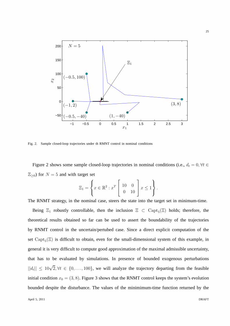
Fig. 2. Sample closed-loop trajectories under th RMNT control in nominal conditions

Figure 2 shows some sample closed-loop trajectories in nominal conditions (i.e.,dt = 0, ∀t ∈

Z≥0) for N = 5 and with target set

Ξ1 =

x ∈ R2 : xT

10 0

0 10

x ≤ 1

.

The RNMT strategy, in the nominal case, steers the state intothe target set in minimum-time.

Being Ξ1 robustly controllable, then the inclusionΞ ⊂ Capt5(Ξ) holds; therefore, the

theoretical results obtained so far can be used to assert theboundability of the trajectories

by RNMT control in the uncertain/pertubed case. Since a direct explicit computation of the

setCapt5(Ξ) is difficult to obtain, even for the small-dimensional system of this example, in

general it is very difficult to compute good approximation ofthe maximal admissible uncertainty,

that has to be evaluated by simulations. In presence of bounded exogenous perturbations

||dt|| ≤ 10√2, ∀t ∈ {0, . . . , 100}, we will analyze the trajectory departing from the feasible

initial conditionx0 = (3, 8). Figure 3 shows that the RNMT control keeps the system’s evolution

bounded despite the disturbance. The values of the minimimum-time function returned by the

April 5, 2011 DRAFT

26

0 5 10 15 20 25 30 35 40 45 50

0

100

200

300

400

500

600

700

800

900

x1

x2

(3, 8)

unfeasible points

Ξ1

N = 5

Fig. 3. Cloud of points obtained by simulating the closed-loop system with bounded perturbations. The transitory unfeasibilities

occurring in presence of disturbances are marked by circles. The feasibility is always recovered in finite-time.

optimization performed along the system’s trajectory are shown in Figure 4.

0 10 20 30 40 50 60 70 80 90 100

0

1

2

3

4

5

t

To M

T(x

t)

Fig. 4. Values of the minimum-time function retruned by the optimization along the system’s trajectory. The circles represent

unfeasible optimization, that is, the target set cannot be reached withinN steps from the correspondent state.

April 5, 2011 DRAFT

27

Several unfeasible points have been reached during the experiment. We remark that the

convenional minimum-time control would not have been able to cope with those unfeasibilities.

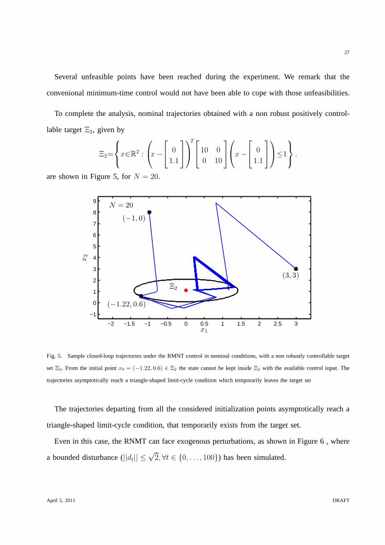
To complete the analysis, nominal trajectories obtained with a non robust positively control-

lable targetΞ2, given by

Ξ2=

x∈R2 :

x−

0

1.1

T

10 0

0 10

x−

0

1.1

≤1

.

are shown in Figure 5, forN = 20.

−2 −1.5 −1 −0.5 0 0.5 1 1.5 2 2.5 3

−1

0

1

2

3

4

5

6

7

8

9

x1

x2

Ξ2

(3, 3)

(−1.22, 0.6)

(−1, 0)

N = 20

Fig. 5. Sample closed-loop trajectories under the RMNT control in nominal conditions, with a non robustly controllabletarget

setΞ2. From the initial pointx0 = (−1.22, 0.6) ∈ Ξ2 the state cannot be kept insideΞ2 with the available control input. The

trajectories asymptotically reach a triangle-shaped limit-cycle condition which temporarily leaves the target set

The trajectories departing from all the considered initialization points asymptotically reach a

triangle-shaped limit-cycle condition, that temporarilyexists from the target set.

Even in this case, the RNMT can face exogenous perturbations, as shown in Figure 6 , where

a bounded disturbance (||dt|| ≤√2, ∀t ∈ {0, . . . , 100}) has been simulated.

April 5, 2011 DRAFT

28

−2 −1.5 −1 −0.5 0 0.5 1 1.5 2 2.5 3

−1

0

1

2

3

4

5

6

7

8

9

x1

x2

Ξ2

(−1, 8)

N = 20

Fig. 6. Sample closed-loop trajectory under th RMNT controlwith bounded perturbations. The trajectory remains bounded in

perturbed conditions despite a non robust positively controllable target set has been used

VII. CONCLUSION

In this work we have proposed a robustified minimum-time control scheme for nonlinear

discrete-time systems with input constraints that admits non robustly controllable target sets.

Given a Lipschitz nonlinear transition map with hard constraints on control inputs, the

reachability properties of the target set have been used to assess the robustness of the minimum-

time control. In particular, the recursive feasibility of the scheme is preserved with non robust

positively controllable target set and in presence of bounded exogenous disturbances.

REFERENCES

[1] V. Kucera, “The structure and properties of time-optimal discrete linear control,”IEEE Transactions on Automatic Control,

vol. 16, no. 4, pp. 375 – 377, 1971.

[2] S. S. Keerthi and E. G. Gilbert, “Computation of minimum-time feedback control laws for discrete-time systems with

state-control constraints,”IEEE Transactions on Automatic Control, vol. 32, no. 5, pp. 432–435, 1987.

April 5, 2011 DRAFT

29

[3] D. Mayne and W. Schroeder, “Robust time-optimal controlof constrained linear systems,”Automatica, vol. 33, no. 12,

pp. 2103–2118, 1997.

[4] Z. Gao, “On discrete time optimal control:a closed-formsolution,” inProc. American Control Conference, 2004, pp. 52–58.

[5] F. Blanchini and S. Miani,Set-Theoretic Methods in Control. Boston: Birkhauser, 2008.

[6] F. Blanchini, “Set invariance in control,”Automatica, vol. 35, no. 11, pp. 1747–1767, 1999.

[7] D. Bertsekas and I. Rhodes, “On the min-max reachabilityof target set and target tubes,”Automatica, vol. 7, pp. 233–247,

1971.

[8] S. Rakovic and D. Mayne, “Robust time-optimal obstacle avoidance problem for constrained discrete-time systems,”in

Proc. of the 44th IEEE Conference on Decision and Control, Seville, Dec 2005.

[9] S. Rakovic, E. Kerrigan, D. Mayne, and J. Lygeros, “Reachability analysis of discrete-time systems with disturbances,”

IEEE Trans. on Automatic Control, vol. 51, no. 4, pp. 546–561, 2006.

[10] I. Kolmanovsky and E. Gilbert, “Theory and computationof invariant sets for discrete-time linear systems,”Math.Probl.

in Engineering, vol. 35, no. 11, pp. 1747–1767, 1999.

[11] F. Blanchini, “Minimum-time control for uncertain discrete-time linear systems,” inProceedings of the 31st IEEE

Conference on Decision and Control, Tucson, 1992, pp. 2629–2634.

[12] ——, “Ultimate boundedness control for discretetime uncertain systems via set-induced lyapunov functions,”IEEE Trans.

on Automatic Control, vol. 39, pp. 428–433, 1994.

[13] D. Q. Mayne and H. Michalska, “An implementable receding horizon controller for stabilization of nonlinear systems,” in

Proc. of the 32nd Conf. on Decision and Control, Honolulu, 1990.

[14] D. Mayne, J. Rawlings, C. Rao, and P. Skokaert, “Constrained model predictive control: Stability and optimality,”

Automatica, vol. 36, pp. 789–814, 2000.

[15] D. Limon, T. Alamo, and E. F. Camacho, “Stability analysis of systems with bounded additive uncertainties based on

invariant sets: Stability and feasibility of mpc,” inProc. American Control Conference, 2002.

[16] L. Magni, D. M. Raimondo, and R. Scattolini, “Regional input-to-state stability for nonlinear model predictive control,”

IEEE Trans. on Automatic Control, vol. 51, no. 9, 2006.

[17] D. Limon, T. Alamo, F. Salas, and E. F. Camacho, “Input to state stability of min-max MPC controllers for nonlinear

systems with bounded uncertainties,”Automatica, vol. 42, pp. 797–803, 2006.

[18] E. Kerrigan and J.M.Maciejowski, “Robust feasibilityin model predictive control: Necessary and sufficient conditions,” in

Proc. of the IEEE Conf. on Decision and Control, 2001, pp. 728–733.

[19] G. Pin and T. Parisini, “Set invariance under controlled nonlinear dynamics with application to robust RH control,” in

Proc. of the IEEE Conf. on Decision and Control, Cancun, 2008, pp. 4073 – 4078.

[20] G. Pin, D. Raimondo, L. Magni, and T. Parisini, “Robust model predictive control of nonlinear systems with bounded and

state-dependent uncertainties,”IEEE Trans. on Automatic Control, vol. 54, no. 7, pp. 1681–1687, 2009.

April 5, 2011 DRAFT

30

[21] E. Kerrigan and J.M.Maciejowski, “Invariant sets for constrained nonlinear discrete-time systems with application to

feasibility in model predictive control,” inProc.IEEE Conf. Decision and Control, 2000.

[22] G. Pin and T. Parisini, “Extended recursively feasiblemodel predictive control of nonlinear discrete-time systems,” in Proc.

IEEE American Control Conference 2010, Baltimore, 2010.

April 5, 2011 DRAFT