Technical paper 1 - icrc.act.gov.au · Technical paper 1: Price elasticity of water demand Tariff...
57
Technical paper 1 Price elasticity of water demand in the ACT Tariff Review 2016 Regulated water and sewerage services Report 1 of 2016, February 2016
Transcript of Technical paper 1 - icrc.act.gov.au · Technical paper 1: Price elasticity of water demand Tariff...

Technical paper 1 Price elasticity of water
demand in the ACT Tariff Review 2016
Regulated water and sewerage services
Report 1 of 2016, February 2016

Technical paper 1: Price elasticity of water demand Tariff Review 2016 i
The Independent Competition and Regulatory Commission is a Territory Authority established under the Independent Competition and Regulatory Commission
Act 1997 (the ICRC Act). The Commission is constituted under the ICRC Act by one or more standing commissioners and any associated commissioners
appointed for particular purposes. Commissioners are statutory appointments and the current Commissioners are Senior Commissioner Malcolm Gray and
Commissioner Mike Buckley. We, the Commissioners who constitute the Commission, take direct responsibility for delivery of the outcomes of the
Commission.
We have responsibilities for a broad range of regulatory and utility administrative matters. We have responsibility under the ICRC Act for regulating and advising government about pricing and other matters for monopoly, near-monopoly and ministerially declared regulated industries, and providing advice on competitive
neutrality complaints and government-regulated activities. We also have responsibility for arbitrating infrastructure access disputes under the ICRC Act.
In discharging our objectives and functions, we provide independent robust analysis and advice.
Our objectives are set out in section 7 of the ICRC Act and section 3 of the Utilities Act 2000.
Correspondence or other inquiries may be directed to the Commission at the following addresses:
Independent Competition and Regulatory Commission PO Box 161
Civic Square ACT 2608
Level 8 221 London Circuit Canberra ACT 2601
We may be contacted at the above addresses, by telephone on (02) 6205 0799, or by fax on (02) 6207 5887. Our website is at www.icrc.act.gov.au and our email
address is [email protected].

Technical paper 1: Price elasticity of water demand Tariff Review 2016 i
Foreword Although the work reported here was done to meet the requirements of the review of tariff structures for water and sewerage services, it forms a natural complement to the work done early in 2015 on the aggregate consumption of water in the ACT. The earlier work looked at total consumption of water across all the customers of Icon Water. This study looks at the behaviour of individual customers.
The clear conclusion that emerges from both studies is that significant changes in water consumption patterns have emerged as a result of the community’s experience of the Millennium Drought. Aggregate water consumption has fallen by around 10GL/a or about 20 per cent. The price elasticity of water demand from separately metered domestic premises has fallen even more dramatically from about -0.3 to about -0.03. The community has sharply reduced its water consumption and has reached the point where further significant reductions would be difficult to achieve. Moreover there is no sign of aggregate demand moving back to pre-drought levels and apparently little likelihood that price reductions would stimulate demand to any significant extent.
From the Commission’s perspective, the earlier study demonstrated its capacity to derive useful results using current methods of time series analysis on a large body of data. This report shows how the Commission can derive useful results using current techniques of panel data analysis and manage an even larger body of complex data.
In both studies, the key data that made the work possible was provided by Icon Water. The Commission gratefully acknowledges the cooperation of Icon Water in providing these datasets to the Commission and assisting in their interpretation.
Since this is the last report that will be issued by the Commission during the stewardship of Commission Buckley and myself, we take pleasure in acknowledging the contribution of the Commission’s staff to the achievements of the Commission over the last five years. We feel we are leaving the Commission a more capable organisation than we found it and trust that it will continue to be an important, independent force in protecting the interests of the ACT community.
Malcolm Gray
Senior Commissioner
29 February 2016

ii Technical paper 1: Price elasticity of water demand
Tariff Review 2016
How to make a submission The technical paper on water demand elasticity in the ACT provides another opportunity for stakeholders to inform the development of the draft report. It will also ensure that relevant information and views are made public and brought to the Commission’s attention.
Submissions may be mailed to the Commission at:
Independent Competition and Regulatory Commission PO Box 161 Civic Square ACT 2608
Alternatively, submissions may be emailed to the Commission at [email protected]. The Commission encourages stakeholders to make submissions in either Microsoft Word format or PDF (OCR readable text format – that is, they should be direct conversions from the word-processing program, rather than scanned copies in which the text cannot be searched).
For submissions received from individuals, all personal details (for example, home and email addresses, and telephone and fax numbers) will be removed for privacy reasons before the submissions are published on the website.
The Commission is guided by and believes strongly in the principles of openness, transparency, consistency and accountability. Public consultation is a crucial element of the Commission’s processes. The Commission’s preference that all submissions it receives be treated as public and be published on the Commission’s website unless the author of the submission indicates clearly that all or part of the submission is confidential and not to be made available publicly. Where confidential material is claimed, the Commission prefers that this be under a separate cover and clearly marked ‘In Confidence’. The Commission will assess the author’s claim and discuss appropriate steps to ensure that confidential material is protected while maintaining the principles of openness, transparency, consistency and accountability.
We may be contacted at the above addresses, by telephone on (02) 6205 0799 or by fax on (02) 6207 5887. The Commission’s website is at www.icrc.act.gov.au.
The closing date for submissions on the issues paper, this and subsequent technical papers is 5 pm, 1 July 2016.

Technical paper 1: Price elasticity of water demand Tariff Review 2016 i
Contents
Foreword i
How to make a submission ii
1 Introduction 1 1.1 Background and purpose of this technical paper 1 1.2 Water prices in the ACT 2 1.3 Review timeline and submission process 4 1.4 Technical paper structure 5
2 Theory and practice 7 2.1 Introduction 7 2.2 The economic model 7 2.3 Econometric implications of block rate structures 10 2.4 Empirical water demand elasticity estimates 17
3 ACT water demand model 20 3.1 Data sources 20 3.2 Unit record preparation 21 3.3 Variables 24 3.4 Estimated model 28
4 ACT elasticity results 33 4.1 Introduction 33 4.2 Residential (RESS) charge class 33 4.3 Units and flats (ACP1) charge class 39 4.4 Commercial (COMM) charge class 40
5 Conclusion 43
Appendix 1 Elasticity of demand definition 45
Appendix 2 Semi-log model results 47
Abbreviations and acronyms 49
References 51

ii Technical paper 1: Price elasticity of water demand
Tariff Review 2016
List of tables
Table 1.1 Icon Water’s water tariffs, 1998–99 to 2015–16 ($, current prices) 3
Table 1.2 Indicative timeline for the tariff review 4
Table 3.1 Icon Water unit record billing data 20
Table 3.2 Price variables 25
Table 3.3 Variables 30
Table 4.1 Significance levels 33
Table A2.1 Semi-log price elasticity of demand results 47
List of figures
Figure 2.1 Household demand − linear budget constraint 8
Figure 2.2 Household demand − nonlinear budget constraint 9
Figure 3.1 Fourier series 27
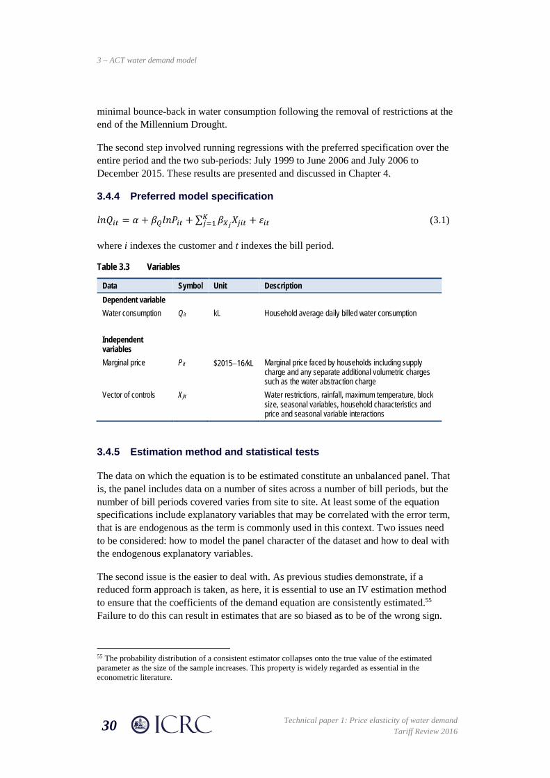
Figure 4.1 Model results, RESS − 1999 to 2015 period 34
Figure 4.2 Seasonal interaction with elasticity estimate, RESS − 1999 to 2015 period 36
Figure 4.3 Model results, RESS − 1999 to 2006 sub-period 37
Figure 4.4 Model results, RESS − 2006 to 2015 sub-period 38
Figure 4.5 Model results, ACP1 − 1999 to 2015 period 40
Figure 4.6 Model results, COMM − 1999 to 2015 period 42
Figure A1.1 Price elasticity of demand 45
List of boxes
Box 2.1 2SLS with IV procedure 17

Technical paper 1: Price elasticity of water demand Tariff Review 2016 1
1 Introduction
1.1 Background and purpose of this technical paper
This technical paper is the second paper published by the Commission as part of its review of Icon Water's water and sewerage services tariff structures. The first publication was an issues paper released by the Commission in November 2015.1
The issues paper introduced the topic of using price to manage water demand as an alternative to, or in conjunction with, other non-price supply-side measures such as temporary water restrictions. The issues paper also raised the matter of using Ramsey pricing to minimise price distortions when setting prices above marginal cost in a systematic manner to recover residual costs.
Using price to manage demand and the application of Ramsey pricing both require an estimate of the price elasticity of demand for water. In the former case, armed with the price elasticity of demand for water, one can calculate the required change in price to achieve a desired reduction in water use.
In the latter case, Ramsey pricing involves deliberate and systematic price discrimination on the basis of elasticities of demand to allow the monopoly business to recover residual costs while minimising the deviations from optimal, that is based on marginal cost pricing, consumption patterns. Customers who are price inelastic are charged a higher price than those who are price elastic, with more of the residual costs recovered from customers who are price inelastic than from the customers with elastic demand.
The purpose of this paper is to estimate the price elasticity of demand for water in the ACT. The primary focus of this paper is on estimating the price elasticity of demand for water by standalone residential households with separate water meters. This residential class of customers forms the majority of Icon Water’s customer base and is the principal target of the ACT Government’s water conservation and temporary water restrictions schemes.
In addition to residential, two other elasticity estimates are undertaken: that for customers in flats and units and that for Icon Water’s commercial customers.
The paper first explores a number of econometric issues relevant to the estimation of the price elasticity of demand in the presence of inclining block tariffs. This includes a review of the theoretical and empirical literature. Second, an econometric water demand model for the ACT is developed, and then specified using unit level water consumption data and a range of price, weather, water restrictions and socio-economic
1 ICRC, 2015a: 1-90. Available for download from: http://www.icrc.act.gov.au/water-and-sewerage/inquiries-and-investigations/.

1 – 293BIntroduction
2 Technical paper 1: Price elasticity of water demand
Tariff Review 2016
variables. The specified model is then used to estimate the price elasticity of demand for water in the ACT for several charge classes.
1.2 Water prices in the ACT
Table 1.1 shows Icon Water’s water tariffs as determined by the Commission since 1998−99, presented in current prices.
Over this period, there have been changes in the structure of the inclining block going from two to three and then back to two pricing tiers. The level of the consumption steps have also changed over time. In addition, there have been several changes in the way in which Icon Water has applied water prices in its billing system. These are discussed in turn below.
1.2.1 Pro rata pricing
Prior to 1 July 2004, the billing system charged prices for all water consumed since the previous meter reading at the prices in effect on the day of the meter reading, regardless of the period in which the water was consumed. For example, a customer with a meter reading on 2 July would pay for all water at the new tariff effective from 1 July. From 1 July 2004, a pro rata billing system was introduced whereby the customer in the example above would pay for the majority of water at the previous rate, with only 1/91 of water being consumed over the quarter billed at the new rate.2
1.2.2 Anniversary dates
Prior to 1 July 2004, the annual water consumption steps under the inclining block tariff were reset on a specified metering anniversary date based on when the meter was installed. This resulted in customers having different anniversary dates. For the purposes of this paper, and for ease of calculation, the Commission has applied a common meter reading anniversary date at the suburb level.3 From 1 July 2004, anniversary dates for all customers were standardised to 1 July each year.4
2 ICRC, 2004: 125. 3 Using the mode of a sample of about 23,580 customer anniversary dates. 4 ICRC, 2004: 126.

1 – 293BIntroduction
Technical paper 1: Price elasticity of water demand Tariff Review 2016 3
Table 1.1 Icon Water’s water tariffs, 1998–99 to 2015–16 ($, current prices)
1998–99 1999–2000 2000–01 2001–02 2002–03 2003–04 2004–05 2005–06 2006–07 2007–08
Fixed charge ($/a) 125.00 125.00 125.00 125.00 125.00 125.00 75.00 75.00 75.00 75.00
Tier 1 price ($/kL) 0.37 0.38 0.38 0.40 0.41 0.43 0.515 0.58 0.66 0.78
Tier 2 price ($/kL) 0.76 0.83 0.86 0.94 0.97 1.05 1.00 1.135 1.29 1.67
Tier 3 price ($/kL) 1.35 1.53 1.74 2.57
Plus water abstraction charge ($/kL)(a) 0.10 0.10 0.10 0.10 0.15 0.20 0.25 0.55 0.55
First consumption step (kL/a) 300 275 250 225 200 175 100 100 100 100
Second step (kL/a) 300 300 300 300
2008–09 2009–10 2010–11 2011–12 2012–13 2013–14 2014–15 2015–16
Fixed charge ($/a) 85.00 89.55 92.08 95.63 99.83 100.00 102.56 101.14 Tier 1 price ($/kL) 1.85 1.95 2.00 2.33 2.43 2.55 2.64 2.60 Tier 2 price ($/kL) 3.70 3.90 4.01 4.66 4.86 5.10 5.29 5.22 Tier 3 price ($/kL) Plus water abstraction charge ($/kL) WAC incorporated directly in prices from 2008–09 First consumption step (kL/a) 200 200 200 200 200 200 200 200 Second step (kL/a)
(a) The water abstraction charge in 2003−04 was $0.10/kL for the first half of the financial year and $0.20/kL for the second half. (b) The Utilities Network Facilities Tax (UNFT) was levied as a volumetric charge in 2007−08.

1 – 293BIntroduction
4 Technical paper 1: Price elasticity of water demand
Tariff Review 2016
1.2.3 Daily pricing
Under an inclining block tariff customers can progress through the volumetric steps of the inclining block tariff either on an annual basis or on a daily basis. Prior to 1 July 2008, the former was applied. Under the annual approach, a customer who consumes a constant volume of water during each quarter above a threshold level will usually receive a larger bill for the final quarter compared to the first quarter of the financial year.
Under daily pricing, the annual price structure is applied on a daily basis at each meter reading. That is, the annual allocation of water in each consumption band is converted to a daily allowance. The daily allowance is then multiplied by the number of days in the billing period to determine the quarterly allocations and hence the quarterly bill. This daily pricing approach was applied by Icon Water from 1 July 2008.5
1.3 Review timeline and submission process
The indicative timeline for the remainder of the review is set out in Table 1.2.
Table 1.2 Indicative timeline for the tariff review
Task Date Release of issues paper 23 November 2015 Release of Technical paper 1: Water demand elasticity 29 February 2016 Release of Technical paper 2: Marginal cost pricing April 2016 Release of Technical paper 3: Trade waste pricing May 2016 Submissions on issues and technical papers close 1 July 2016
Release of draft report August 2016
Public forum September 2016 Workshops September 2016 Submissions on draft report close September2016 Final report November 2016
The closing date for submissions on this and the other technical papers is 1 July 2016. Details on how to make a submission are shown in the How to make a submission section at the front of this paper. Stakeholders are free to make submissions on any of the papers at any time before the closing date and may make multiple submissions if so desired. Written submissions received by the closing date will be considered in the development of the draft report.
5 ICRC, 2008: 135.

1 – 293BIntroduction
Technical paper 1: Price elasticity of water demand Tariff Review 2016 5
A separate submission process will be undertaken to allow stakeholders to respond to the draft report. Details on this submission period will be provided at the time the draft report is published.
1.4 Technical paper structure
The remainder of the issues paper is structured as follows:
• Chapter 2 discusses the economic theory underpinning the estimation of the price elasticity of demand and presents an economic model of household demand for water. A range of econometric issues relevant to the estimation of elasticities in the presence of inclining block tariffs is also considered, in addition to review of empirical estimates from water demand studies.
• Chapter 3 describes the data used for estimation purposes, discusses the unit record extraction process, and presents the preferred model specification.
• Chapter 4 presents and discusses the model results.
• Chapter 5 concludes with the key policy implications for scarcity and Ramsey pricing.
• Appendix 1 provides a definition of price elasticity of demand.
• Appendix 2 presents the model results from the semi-log form of the preferred model specification.

Technical paper 1: Price elasticity of water demand Tariff Review 2016 7
2 Theory and practice
2.1 Introduction
Economists have been publishing empirical estimates of the price elasticity of demand for water for more than 50 years.6 At first blush, estimating water demand seems a fairly simple matter of regressing water consumption against the water price and a range of other factors that might influence water consumption, such as climate or income levels.
However, as one delves deeper, it soon becomes evident that there are some econometric difficulties that need to be addressed. Perhaps the most critical relates to the non-linearities and discontinuities inherent in the block rate tariff structures commonly used by water utilities. Conveniently, this issue has spawned a sizeable and readily accessible literature on the econometric issues associated with estimating demand functions for water and other commodities with similar tariff structures, such as electricity, and the wage elasticity of labour supply under progressive taxation.
This chapter starts by considering the economic basis for the water demand function. It then provides a Cook’s tour of particular issues associated with estimating water demand functions, including a review of the relevant literature. The chapter concludes with a brief review of the empirical estimates literature, including previous estimates of the demand elasticity for water in the ACT.
2.2 The economic model
2.2.1 Introduction
The first step in estimating the price elasticity of demand for water is to consider an appropriate economic model of demand for water.
Espey et al. (1997), in their meta-analysis of the price elasticity of residential demand for water, noted that water can be used in a number of different ways, which can potentially result in different demand functions for different uses. As such, it is important to first classify water use into relevant categories such as residential, industrial and agricultural. In particular, it is important to avoid pooling the quantity of water demanded across categories as this ‘imposes the restriction that the specifications are homogeneous, no matter what type of use.’7
6 For example, see Howe and Linaweaver, 1967: 13-32. 7 Espey, Espey and Shaw, 1997: 1370.
2 – Theory and practice
8 Technical paper 1: Price elasticity of water demand
Tariff Review 2016
In this paper, the Commission is primarily concerned with estimating the price elasticity of demand for residential water in the ACT, more specifically for those residential properties that are separately metered.
In order to develop an economic model of water demand by residential users, we turn to the classical theory of demand and the maximisation of household utility subject to a budget constraint. The utility that a household derives from water is largely related to the direct use of that water for indoor uses (drinking, washing and flushing) and outdoor uses (irrigating gardens). This generally contrasts with water use in the industrial sector which is likely to be primarily a derived demand:
Demand for water in production (agricultural or industrial uses) is likely a derived demand, where the demands are input demand functions derived via a profit maximization or cost minimization problem.8
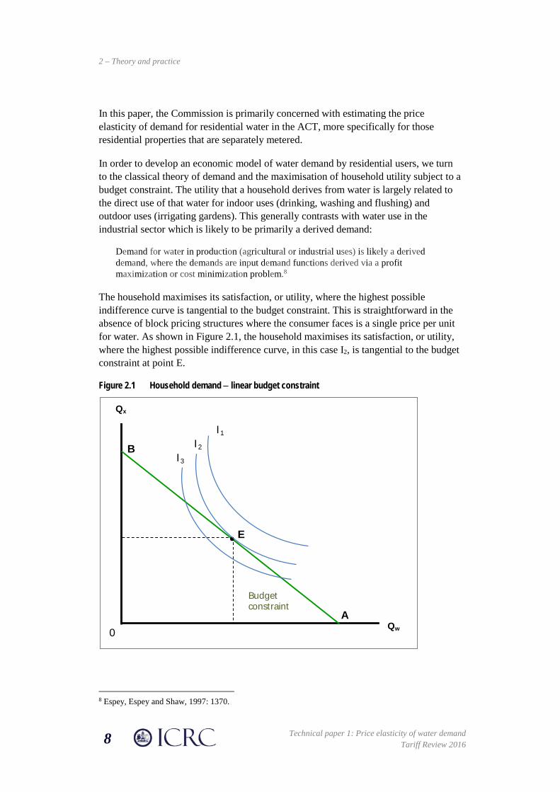
The household maximises its satisfaction, or utility, where the highest possible indifference curve is tangential to the budget constraint. This is straightforward in the absence of block pricing structures where the consumer faces is a single price per unit for water. As shown in Figure 2.1, the household maximises its satisfaction, or utility, where the highest possible indifference curve, in this case I2, is tangential to the budget constraint at point E.
Figure 2.1 Household demand − linear budget constraint
8 Espey, Espey and Shaw, 1997: 1370.
Qx
Qw
Budget constraint
I1
I2
I3
E
0
B
A
2 – Theory and practice
Technical paper 1: Price elasticity of water demand Tariff Review 2016 9
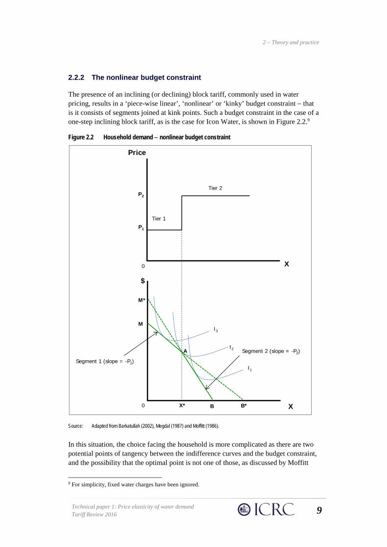
2.2.2 The nonlinear budget constraint
The presence of an inclining (or declining) block tariff, commonly used in water pricing, results in a ‘piece-wise linear’, ‘nonlinear’ or ‘kinky’ budget constraint − that is it consists of segments joined at kink points. Such a budget constraint in the case of a one-step inclining block tariff, as is the case for Icon Water, is shown in Figure 2.2.9
Figure 2.2 Household demand − nonlinear budget constraint
Source: Adapted from Barkatullah (2002), Megdal (1987) and Moffitt (1986).
In this situation, the choice facing the household is more complicated as there are two potential points of tangency between the indifference curves and the budget constraint, and the possibility that the optimal point is not one of those, as discussed by Moffitt
9 For simplicity, fixed water charges have been ignored.
$
0
M
Price
X0
Tier 1
Tier 2
I1
M*
A
X* B B*
I3
P1
P2
Segment 1 (slope = -P1)
Segment 2 (slope = -P2)I2
X
2 – Theory and practice
10 Technical paper 1: Price elasticity of water demand
Tariff Review 2016
(1990). That is, the household may choose between the tangency associated with segment 1 or segment 2, or the kink point of the budget constraint shown in Figure 2.2.
This economic choice can also be set out algebraically, following Megdal (1987). Suppose the consumer maximises a strictly quasi-concave utility function U(X,Y), where X and Y are two goods, subject to a nonlinear budget constraint. Let the price of Y be set equal to 1, M be the money income of the consumer, P1 be the price of good X for the first X* units purchased, and P2 be the price of good X for units beyond X*. We assume that P1 < P2, in line with the convex budget set arising from an inclining block utility tariff.
The budget constraint can be written as:
𝑀𝑀 = 𝑃𝑃1𝑋𝑋 + 𝑌𝑌 if 𝑋𝑋 ≤ 𝑋𝑋∗ (1)
𝑀𝑀 = 𝑃𝑃1𝑋𝑋∗ + 𝑃𝑃2(𝑋𝑋 − 𝑋𝑋∗) + 𝑌𝑌 (2)
= (𝑃𝑃1 − 𝑃𝑃2)𝑋𝑋∗ + 𝑃𝑃2𝑋𝑋 + 𝑌𝑌 if 𝑋𝑋 > 𝑋𝑋∗ (3)
Megdal (1987) notes that an individual will choose X* if the utility maximizing quantity of X subject to the budget constraint P1X + Y = M is greater than or equal to X* and the utility maximizing quantity of X subject to P2X + Y = M* is less than or equal to X*.10 M* is often called the household’s virtual or imputed income.
2.3 Econometric implications of block rate structures
The difficulties for demand estimation arising from the nonlinearities and discontinuities consequent upon block rate pricing have generated an econometric literature that can be broadly split into two streams.
The first, and earliest, relates to the behaviourally consistent specification of prices in water demand models. The focus of this debate is on whether the price variable in a demand equation should be the marginal price the consumer pays, or the average price. Howe and Linaweaver (1967) are perhaps the earliest contributors to this debate. Following the work by Taylor (1975) and Nordin (1976) on electricity demand, attention turned to the inclusion of a difference variable in the demand equation to account for the intra-marginal effects caused by block rate pricing.11 Later
10 Megdal, 1987: 244. 11The difference variable, also known a rate structure premium, is the difference between the total bill and what the bill would have been if all consumption were charged at the marginal block price. This is discussed in more detail in section 2.3.1.

2 – Theory and practice
Technical paper 1: Price elasticity of water demand Tariff Review 2016 11
contributions included Shin (1985), who introduced a perceived price variable in addition to the marginal price.12
The second and more recent stream moved on to the choice of estimating technique to deal with the price endogeneity problem resulting from price varying with the quantity of water consumed under a block tariff. This debate is principally about the choice between using structural or reduced-form econometric estimation techniques.13
Deller et al. (1986) noted that the two debates are not unrelated since empirical validation of consumer behaviour requires application of appropriate estimating techniques.
These two streams are navigated in turn.
2.3.1 The marginal versus average price debate
A central tenet of microeconomic theory is that well-informed, rational households will consider marginal prices when making their budget allocation decisions. Nevertheless, there has been considerable debate concerning the "correct" price to include in empirical models of household demand for public utility services.14
Economic theory suggests that consumers react to marginal prices when making consumption decisions. However, there are a number of characteristics of the water market, including the market in the ACT, that indicate this may not necessarily be the case. These characteristics are a result of the manner in which water consumption is measured and bills calculated and presented to customers.
In the ACT water consumption is measured using accumulation meters. These meters simply record the volume of water used, with customers billed on a quarterly basis. Accumulation meters store no information about when consumption has occurred and are often in inaccessible locations, making it impractical for customers to monitor their own consumption. This results in customers being generally unaware of how much they have consumed. The only time at which customers receive information about their consumption is on receipt of a bill, which typically covers the preceding three-month period. Because water customers are unaware of their level of consumption (and therefore the tier price to which they are exposed), they may be unaware of the price they are being charged.
This situation differs from that which exists for products provided in a competitive market, for example, petrol. Motorists purchasing petrol know the price they face in
12 The perceived price variable, discussed in more detail in section 2.3.1, is a function of average price, marginal price and a price perception parameter. 13 The terms structural and reduced form originated in the Cowles Commission work on simultaneous equation models. More recently, the terminology has been used to describe models that combine economic theories with statistical models. Such models are referred to as structural econometric models as described in Reiss and Wolak, 2007: 4280-4415. 14 Carter and Milon, 2005: 265.

2 – Theory and practice
12 Technical paper 1: Price elasticity of water demand
Tariff Review 2016
advance and determine their level of consumption based upon that knowledge. In that situation it is reasonable to consider that consumption decisions are based on an analysis of the marginal price per litre of petrol. However, water customers, who receive their bills after consumption has occurred, may base their future consumption decisions on an analysis of the most recent available information. This would mean that customers may make consumption decisions based upon an analysis of average costs calculated from recent bills.
Ito (2014) cites two alternatives to marginal price that customers may respond to when faced with nonlinear price schedules. The first is the expected marginal price, which Koichiro argues is a rational response in the presence of uncertainty about consumption. The second is average price:
Alternatively, consumers may use average price as an approximation of marginal price if the cognitive cost of understanding complex pricing is substantial. This suboptimization is described as “schmeduling” by Liebman and Zeckhauser (2004).15
There have been a number of empirical studies in the economics literature examining the question of whether consumers respond to marginal or average price. Shin (1985) examined residential electricity consumption under a declining block tariff and found that the empirical evidence supported the hypothesis that customers who are not well-informed respond to perceived average price as opposed to marginal price.
A later study by Nieswiadomy and Molina (1991) found that residential water customers responded to marginal price when faced with inclining block structures and average price when responding to decreasing block structures. A further study by Nieswiadomy (1992), which among other things investigated the effect of price structure on residential water demand, confirmed the Shin hypothesis that customers react more to average price than marginal price.
The study by Ito (2014) on customer response to nonlinear electricity prices using household-level panel data, found ‘strong evidence that consumers respond to average price rather than marginal or expected marginal price.’16
The mere existence of a debate about whether customers respond to marginal or average price has important consequences. Clearly, if consumers appear not to respond to marginal prices there is limited benefit in setting prices with reference to marginal costs.
Taylor (1975), in a study of electricity demand, suggested that under block rate pricing the explanatory variables should include both marginal and average price. Subsequently, Nordin (1976) argued that Taylor's specification should be modified to
15 Ito, 2014: 538. 16 Ito, 2014: 537.

2 – Theory and practice
Technical paper 1: Price elasticity of water demand Tariff Review 2016 13
include a difference variable to account for the effects of intramarginal rates and fixed fees:
It is appropriate to use (in addition to marginal price) a variable equivalent to a lump-sum payment the customer must make before buying as many units as he wants, at the marginal price.17
Nordin defined the difference as the total bill minus what the bill would have been if all units had been purchased at the marginal price.
Shin (1985), in a study into effect of the price information problem on electricity consumers' price perceptions, found empirical results that support the hypothesis that consumers respond to average price perceived from the electricity bill rather than the marginal price.
2.3.2 Techniques to deal with the endogeneity problem
Introduction
In his seminal paper on electricity demand, Taylor (1975) commented on the issue of the theoretical plausibility of electricity demand functions:18
It has been well known since the paper of Houthakker that the presence of a price schedule has important econometric implications, but the literature has focused rather narrowly on the question of the type of price−marginal or average−that should be included in the demand function. That the price schedule has implications for the equilibrium of the consumer−and therefore for the demand function itself−has not been systematically investigated.19
The principal consequence of the kinked budget constraint for the equilibrium of the consumer derives from the price endogeneity problem. The endogeneity arises because price varies with the quantity of water consumed rather than being a strictly exogenous variable in the demand function.
The key implication is that, as demonstrated by Moffitt (1990), because the demand function is discontinuous, with jumps at the kink points where equilibrium switches from one facet of the budget constraint to another, it can be difficult to predict the effect of price or income impacts that cause a consumer to move between kinks.
The comparative statics of consumer demand as enshrined in textbooks-most notably, the negative effect of price on quantity demanded under well-known conditions and the presumed positive effect of income on the quantities demanded of most goods−holds up in the presence of kinked budget sets only "within" segments. If the
17 Nordin, 1976: 719. 18 Block tariffs are common in the electricity industry. 19 Taylor, 1975: 76.

2 – Theory and practice
14 Technical paper 1: Price elasticity of water demand
Tariff Review 2016
price or income change in question causes the consumer to change segments or kinks, there are, in general, no unambiguous directions of predicted effect.20
Moffitt (1990) also noted that a particular marginal price is relevant to the consumer’s decision only when he or she is consuming in the block to which it relates. That is, it governs behaviour within that block but does not determine why the consumer consumes in that block as opposed to some other block.
Olmstead (2009) identified another problem with kinky budget constraints that relates directly to the impact of own consumption on the marginal price. The issue here is that because the marginal price depends on the quantity of the good consumed and there is a random component to the determination of the quantity, there will be a non-zero covariance between the error term and the variable measuring marginal price.21 In these circumstances, applying ordinary least squares (OLS) to the standard linear specification will produce biased and inconsistent parameter estimates.
A number of econometric estimation techniques have been applied to account for endogenous prices when estimating demand functions. Two of the most common can be broadly distinguished as structural or reduced-form estimation techniques.
Structural demand estimation
The structural approach to dealing with piecewise budget constraints was developed by labour economists to estimate the wage elasticity of labour supply under progressive taxation.
In a ground-breaking paper, Burtless and Hausman (1978) developed such an approach to modelling labour supply that takes into account nonlinearities in the budget constraint due to progressive marginal tax rates. Burtless and Hausman (1978) note that:
Most econometric studies of labor supply assume that the most preferred level of work effort for an individual depends on a single wage rate that is independent of the chosen level of hours of work. Thus the endogeneity of the net wage rate is ignored. When it has been considered, only reduced-form estimates have been computed. These estimates have the disadvantage that they depend on the particular sample information used and cannot be used to evaluate the expected effect of policy changes.
Burtless and Hausman (1978) argued that the parameter estimates derived from their structural model, in which individual choice depends on all net wages which comprise the budget set, is a better way to evaluate policy changes. Moffitt (1990) noted that the main innovation of the Burtless and Hausman (1978) approach was to include two rather than one error term in the econometric model: one representing unobserved heterogeneity of preference and therefore accounting for variation in individual utility
20 Moffitt, 1990: 121. 21 Megdal, 1987: 243.
2 – Theory and practice
Technical paper 1: Price elasticity of water demand Tariff Review 2016 15
functions, and the other representing the optimisation error arising because individuals cannot fine-tune their hours of work precisely.22
Dalhuisen et al. (2003) argued that, in general, the modelling and studies undertaken in relation to the marginal versus average price debate and the endogeneity issue do not explicitly model the consumer’s position on the demand curve.
Hausman (1983) also raised concerns with using simplified reduced−form approaches that rely on local elasticity estimates to analyse changes from income tax reform proposals, noting that such calculations often ignore the considerable heterogeneity of the population response.
Other advocates of the structural approach, such as Olmstead (2009), argue that this approach − of which discrete/continuous choice (DCC) modelling is one example − has two main advantages over reduced-form approaches. The first is that, in theory, they can produce unbiased and consistent estimates of parameters of interest, like price elasticity. Second, they are consistent with utility theory and, therefore, result in demand curves that provide a sound basis from which to perform welfare analysis.23 Olmstead (2009) further noted that reduced-form approaches ‘can incorporate only limited aspects of the piecewise-linear budget constraint.’24
The primary downside of structural approaches is that they are more complicated to implement than simpler reduced-form approaches, which may be the reason that they are rarely implemented in water demand analysis. Olmstead (2009) noted that ‘of 400 price elasticity studies of water demand produced between 1963 and 2004, only three employed DCC models.’25
Structural approaches, such as that championed by Burtless and Hausman (1978), generally employ maximum likelihood estimation (MLE) methods to econometrically estimate the demand function.26 Moffitt (1986) noted:
As is frequently the case with highly nonlinear models, maximum likelihood and nonlinear least squares are attractive estimation methods because they generally provide estimates with the desirable large-sample properties of consistency, asymptotic normality, and asymptotic efficiency.27
22 Moffitt, 1990: 134. 23 Olmstead, 2009: 84. 24 Olmstead, 2009: 85. 25 Olmstead, 2009: 85. 26 There are two common methods of parameter estimation used in regression analysis, OLS and MLE. The OLS method estimates parameters by minimising the sum of the squared residuals of a set of observations. MLE methods estimate the unknown parameters in such a manner that the probability of observing the given data is as high as possible. OLS is the more common method used in regression analysis as it intuitively appealing and mathematically simpler to apply than MLE methods. 27 Moffitt, 1986: 320. For a detailed treatment of the properties of MLE methods see Greene, 2012: 118.
2 – Theory and practice
16 Technical paper 1: Price elasticity of water demand
Tariff Review 2016
Moffitt (1986) provides a useful review of the application of maximum likelihood methods when estimating demand in the presence of a kinked budget constraint. Moffitt (1986) also noted that structural approaches using maximum likelihood methods are fairly common in the estimation of consumer demand equations derived from piecewise-linear budget constraints in studies of tax and transfer programs.
Reduced-form demand estimation
One of the most common reduced-form estimation techniques employed in estimating water demand functions is the instrumental variables (IV) approach.
A solution to the problem of the correlation between an independent variable and the error term is to construct an instrumental variable − a variable correlated with the independent variable in question but uncorrelated with the error term.28 In a similar vein, Deller et al. (1986) stated:
In short, the goal of the instrument is to provide a proxy for the troublesome variable(s). In the study of water service demand these are the price variables. The instrument should fulfill the requirement of being uncorrelated with the error structure while at the same time be correlated with the stochastic regressor.29
The IV approach seems to have originated with the work of Sewall Wright in the late 1920s.30 In the 1950s, Theil (1992) and Basman (1957) independently developed a method known as two stage least squares (2SLS) for estimating a single, over identified equation from a simultaneous equations model.31 It turns out that 2SLS is a form of IV.32 The IV approach collapses the two stages of the 2SLS into a single step, which is more convenient for calculation. The 2SLS presentation of the estimator, shown in Box 2.1, provides a more intuitive justification for the procedure.
28 Wooldridge (2002) notes that the statement that the instrumental variable is correlated with the troublesome independent variable is not quite correct. Rather, the instrumental variable is partially correlated with the independent variable in question once the other independent variables in the equation have been netted out (Wooldridge, 2002: 84). 29 Deller, Chicoine and Ramamurthy, 1986: 336. 30 See Epstein, 1989: 94–107 for a discussion of the origins of IV and the work of Sewall Wright 31 See Theil, 1992: 65-107 and Basman, 1957: 77-83. 32 For a clear explanation of the derivation of the two estimators and a demonstration of their equivalence, see Goldberger, 1964: 284-7 and 329-36.

2 – Theory and practice
Technical paper 1: Price elasticity of water demand Tariff Review 2016 17
Box 2.1 2SLS with IV procedure
Step 1: Identify the demand equation
Start with the demand equation in which a troublesome explanatory variable is correlated with the stochastic error term.
Step 2: Identify instrumental variables
Identify an instrumental variable that is correlated with the explanatory variable in question but uncorrelated with the error term.
Step 3: First stage regression
Use OLS to regress the troublesome explanatory variable against all of the other explanatory variables in the equation as well as the instrumental variable.
Step 4: Second stage regression
Use OLS to regress the dependent variable from the original equation against the non-troublesome explanatory variables and the in-sample forecast of the troublesome explanatory variable from the first stage regression.
Step 5: Estimate the variance of the error term
The variance of the error term in the original equation must be estimated, not from the second stage residuals, but from residuals calculated using the second stage parameter estimates and the original values of the troublesome explanatory variable.
Examples of studies that have applied instrumental variable techniques include Deller et al. (1986), Nieswiadomy and Molina (1989), Barkatullah (2002), McNair (2006) and Grafton et al. (2011), the latter two in the estimation of the elasticity of demand for water in the ACT. McNair (2006) used Icon Water’s (then ACTEW) regulatory revenue requirement as the instrumental variable. Grafton et al. (2011) used a measure reflecting what the price variable would be, on average, if the tiered pricing structure for the current period were applied to the full distribution of consumption that was observed across the full dataset for a given consumer type (excluding present year consumption).
The choice of modelling approach for this study is considered further in section 3.4.1.
2.4 Empirical water demand elasticity estimates
There has been a significant number of empirical studies undertaken on the price elasticity of demand for residential water in particular and, primarily in the United States of America.
2 – Theory and practice
18 Technical paper 1: Price elasticity of water demand
Tariff Review 2016
Espey et al. (1997) and Dalhuisen et al. (2003) undertook meta-analyses of estimates of residential water demand across a wide range of empirical studies. Using data from 24 journal articles published between 1967 and 1993, Espey et al. (1997) calculated a median demand elasticity of -0.38 and -0.64 for the short and long-run, respectively.33 Using data from 64 studies mostly concerned with short-run elasticities, Dalhuisen et al. (2003) found a sample mean of -0.41, a median of -0.35 and a standard deviation of 0.86.34
Worthington and Hoffman (2008), reviewing 37 studies published since 1980, found that:
Almost without exception, the estimated price elasticities are negative and inelastic (less than one), signifying the percentage reduction in the quantity of residential water demanded is less than proportionate to the percentage increase in price.35
Worthington and Hoffman found that while some estimates are very low, many more lie in the range of 0.25 to 0.75, and conclude that price elasticity estimates are generally found in the range of zero to 0.5 in the short-run and 0.5 to unity in the long-run.
Grafton et al. (2009) undertook a cross-country analysis of residential water demand utilising data from 1,600 households across ten countries. The study found that for all ten countries price elasticity of demand is inelastic, ranging from a low of -0.33 for Norway to a high of -0.88 for Italy with an average across the entire sample of -0.56.36
A number of ACT-specific studies have been undertaken over last 20 years. Graham and Scott (1997) calculated a short-term price elasticity of residential demand for water of -0.22.37 McNair (2006) calculated a price elasticity of demand with a mean across all suburbs of -0.1251, and varying between -0.1035 and -0.1621 for high and low-income suburbs, respectively.38 The most recent study, that by Grafton et al. (2011), short-run elasticity point estimate of -0.16, with a range of -0.10 to -0.18.39
Dalhuisen et al. (2001) found that the use of summer data as compared to year-round data leads to a significantly more elastic price elasticity, with the effect on income elasticities is even higher.40 Renwick and Green (2000) also found that demand is more
33 Espey, Espey and Shaw, 1997: 1371. 34 Dalhuisen, Florax, de Groot and Nijkamp, 2003: 295. 35 Worthington and Hoffman, 2008: 9. 36 Grafton, Kompas, To and Ward, 2009: 10. 37 Graham and Scott, 1997: 11. 38 McNair, 2006: 39. 39 Grafton, Kompas and Ward, 2011: 16. 40 Dalhuisen, Florax, De Groot and Nijkamp, 2001: 15.

2 – Theory and practice
Technical paper 1: Price elasticity of water demand Tariff Review 2016 19
elastic in the summer months, with an elasticity of -0.20 compared to -0.16 across the entire year.41 Renwick and Green conclude that:
These results suggest that price policy will achieve a larger reduction in demand during summer months or in communities with larger irrigated landscaped areas, all other factors held constant.42
41 Renwick and Green, 2000: 49-50. 42 Renwick and Green, 2000: 51.

3 – ACT water demand model
20 Technical paper 1: Price elasticity of water demand
Tariff Review 2016
3 ACT water demand model
3.1 Data sources
The Commission used a range of data sources for this analysis. The bulk of the data was provided by Icon Water in the form of a 10 per cent sample of unit record billing data for the period 1999 to 2015, stratified by charge class. Table 3.1 shows the breakdown of the sample. The residential charge class (RESS) makes up the vast majority of the sample at 87 per cent, followed by Commonwealth Government residential (GOVR) with 6 per cent and residential units and flats (ACP1) with about 2 per cent.
Table 3.1 Icon Water unit record billing data
Charge class Description Dwelling type Sample observations
Percentage of sample
RESS Residential Houses 565,806 87 GOVR Government residential Houses 37,723 6 ACP1 All common properties / res-com Units/flats 14,909 2 COMM Commercial Non-residential 15,295 2 MIS2 City parks (non-school) Non-residential 2,363 0 SCCH Schools and churches Non-residential 1,701 0 GOVF Government flats Units/flats 1,760 0 HOBC Hospitals and benevolent
charities Non-residential 746 0
RESF Residential flats Units/flats 665 0 RCP2 Residential common properties Units/flats 336 0 RESD Residential dual occupancy Units/flats 406 0 GOVD Government dual occupancy Units/flats 242 0 ECCR Ecclesiastical residential Houses 193 0 CCP2 Commercial common property Non-residential 127 0 Sub-total 642,272 Other minor charge classes 9,781 2 Grand-total 652,053
The unit records included data on metered water consumption, consumption charges, total water and sewerage services bill, bill date, meter read from and read to dates, customer address and suburb. A rental indicator was provided by cross-matching the customer’s address with ActewAGL Retail electricity billing records. In addition, block size was provided by cross-matching residential addresses to ACT Government planning data. Icon Water also provided data on historical water restrictions.
3 – ACT water demand model
Technical paper 1: Price elasticity of water demand Tariff Review 2016 21
Daily rainfall and maximum temperature data were drawn from observations by the Bureau of Meteorology (BOM) at Canberra Airport Comparison weather station (070014) and Canberra Airport weather station (070351).
A range of socioeconomic suburb-level data was obtained from the Australian Bureau of Statistics (ABS) 2011 Census data. This included data on household size, age and income. Consumer price index data was also obtained from the ABS.
3.2 Unit record preparation
The unit record data was provided in the form of a 10 per cent sample taken directly from the database underpinning Icon Water’s billing system. Since the purpose of this database is to provide support for the administration of Icon Water’s customer accounts, it contains information about bill corrections and amendments in a form that make it unsuitable for direct use as a source of information on water consumption. The data on water consumption needs to be extracted from the broader set of information contained in the unit record sample as provided by Icon Water.43
The units in the unit record data are sites at which water is provided by Icon Water, associated with entities, for example households or firms, that will be liable to pay for the water provided. The unit record data can be broken into blocks with all the data within each block relating to a single site. As detailed in the previous section, each record within each block provides data about the water consumption at a particular site within a period, the bill period, specified by the read from and read to dates in the record. Normally, the read to date tells the date of a water meter reading and the read from date is the day following the previous meter reading. In some cases, however, these dates relate to other events such as the commencement or termination of an account or the revision of a bill.
Each block then provides a billing history for a particular site. For the purposes of this report, the records within a block, when placed in historical sequence using the date information provided in the record should provide a continuous history of water consumption at the site in question. The continuity of the history provides some assurance of the integrity of the data and it enables the calculation of cumulated consumption over the course of a year, which is required for the calculation of some of the definitions of the water price tested in this report.
Since the length of the bill period varies, we calculate daily consumption to provide a standardised measure of water demand over each bill period. For the purpose of estimating a demand function, we require the water consumption data to represent normal water consumption behaviour, that is, behaviour that is consistent with the 43 Grafton et al. (2011) confronted similar issues in using unit record data from Icon Water’s billing database. The process adopted to deal with these issues in that study seems less systematic than the one described here. It is not clear from the information available to the Commission, however, that the records used in this earlier study contained information about meter read from and read to dates. Without that information, the extraction process described here would not have been possible.

3 – ACT water demand model
22 Technical paper 1: Price elasticity of water demand
Tariff Review 2016
demand equation and not behaviour which has been strongly influenced by other factors, such as an interruption to the occupancy of the site to allow some redevelopment activity. Where records can be identified that seem likely to have been subject to such extraneous influences, it is desirable to exclude them from the dataset used for estimating the demand function, even though such records remain part of the continuous billing history.
As Table 3.1 shows, the number of records to be processed is considerable. It is not, therefore, possible to analyse the unit records individually. Accordingly, an extraction process has been developed using a sequence of database queries written in Structured Query Language (SQL) to extract the required information from the raw sample database provided by Icon Water.44 This process was developed in a series of steps, with irrelevant data being dropped or adjustments made to records before further analysis to identify the next step necessary to advance the process. The extraction process was developed using the subset of records in the RESS charge class as this was by far the largest and likely to be the most complex subset of records.
In its final form the extraction process consists of the following steps. First, sites for which we do not have block size information or which are located in suburbs for which we do not have socioeconomic data are removed. Next, the few records relating to water consumption that occurred before 1 July 1999 are removed as this is the start date for some of our economic data. Then, the records that fail to show any water consumption and sometimes occur for a few periods preceding the commencement or following the termination of supply are removed. The next step is to identify duplicate records, that is, groups of records that relate to the same billing period. For these, the invoice number is used to identify the last entry and presumable the last bill and the older records are removed. Duplication can also occur when a record with a later invoice number shares a read from or to date with a record bearing an earlier invoice number. This form of duplication is dealt with in the same way.
The next steps in the extraction process deal with overlapping records. These occur when a billing record with a read to date after that of another record has a read from date earlier than the read to date of the other record. That is, their bill periods overlap. Sometimes one record of the pair has no entry or a zero entry for water consumption. Such records are removed. Sometimes a record will overlap both a record with an earlier read from date and one with a later read to date, while the records thus overlapped form a continuous sequence. Such bridging records are also removed. Examination of the remaining overlapping records suggests that they be broken into two groups: those where the overlap is large, greater than 15 days, and seems to be more related to bill administration than the measurement of water consumption and 44 SQL is a widely used tool for managing and analysing databases. It is defined in ISO/IEC 9075 and information about it can be found in many places, e.g. at http://www.w3schools.com/sql/. Icon Water provided the unit record data to the Commission in a spreadsheet as this was the most convenient way to migrate the data between the two organisations. The Commission then imported the data into a database for analysis and extraction of the relevant information, ultimately importing the relevant data into the statistical packages used for estimating the demand function. Both Microsoft Access and PostgreSQL database engines were used at various stages of the extraction process.

3 – ACT water demand model
Technical paper 1: Price elasticity of water demand Tariff Review 2016 23
those where overlap is small, no greater than 15 days. Records in the former group are removed and the read from dates of records in the latter group are adjusted to remove the overlap.
Attention then turned to sites with gaps in their billing histories. Since we have no information about what water consumption took place during nor any indication that there were meter readings that covered these periods, it has been assumed, for the purposes of the continuous history, that water consumption was zero across these gaps. The read from date of the following record has been adjusted to remove the gap. Since the gap suggests that there may have been unusual features, including the operation of extraneous factors, over the period covered by the gap, the adjusted record has been marked as not for inclusion in the estimation dataset.
Further examination of the data after these operations have been completed reveals that there are some sites that have a rather erratic pattern of zero, negative and empty readings for water consumption in records from the earlier part of the 2000s, but with apparently normal patterns of consumption from about the middle of 2007 onwards. Since cumulated consumption ceases to play any role in determining any of the definitions of water price from 1 July 2008 onwards, use can be made of the records for these sites from that date onwards. Records for these sites before that date are deleted.45 Any remaining records showing negative water consumption are retained in the continuous billing history as being the only information we have about water consumption in the relevant period, but are marked for exclusion from the estimation dataset.
At this stage in the extraction process, every site has a continuous billing history, with the read from date in each record, except the first, being one day later than the read to date in the preceding record. The length of this history varies from site to site. The longest billing histories contain 65 records and stretch over the entire data period. The shortest relate to newly established dwellings and may have only a handful of records.
Bill periods vary across records, but the overwhelming majority are close to the 91 days, which is the average length of the bill period for meters read quarterly. Some variation in the actual bill period would, of course, be expected because of the occurrence of weekends, public holidays and variations in the availability of meter readers. Analysis of the records thus far included in the estimation dataset shows that 97.5 per cent have billing periods within plus or minus 10 days of 91 days. We accept these records as likely to represent normal consumption behaviour as defined above. The remaining 2.5 per cent of these records have bill periods that range from 2 to 396 days, suggesting the influence of extraneous factors on water consumption. None of these records are included in the estimation dataset.
Final housekeeping, including removing any sites that do not have any records in the estimation dataset, is carried out before checking that every included site has a 45 These records could have been kept, but marked not for inclusion in the estimation dataset. This would, however, have meant that these records were not used for any purpose and it is simpler to delete them.

3 – ACT water demand model
24 Technical paper 1: Price elasticity of water demand
Tariff Review 2016
continuous billing history, that there are no records with empty entries for water consumption and that all records with zero or negative water consumption are marked for exclusion from the estimation dataset.
The operations described in the preceding paragraphs yield a set of 539,347 records with a continuous billing history at each of 10,096 sites. Of these some 521,919 records or 96.8 per cent are marked for inclusion in the estimation dataset. Overall, 26,459 records or 4.7 per cent of the original sample have been culled to arrive at a set of continuous billing histories and 43,887 records or 7.8 per cent have been culled to arrive at an estimation dataset.46
The extraction process developed to deal with records from the RESS charge class has also been successfully employed to extract relevant information from records included in the ACP1 and COMM charge classes.
3.3 Variables
3.3.1 Water consumption
Average daily household water consumption in kilolitres was obtained by dividing each quarterly bill consumption volume by the billing period. In the preferred model specification a logarithmic transformation was applied (logWater_cons).
3.3.2 Water price
As discussed in Chapter 2, there is debate about the price to which water consumers respond. While the debate is largely about whether consumers respond to marginal or average price, there is the separate question of which measure of marginal price should be applied when considering a marginal response.
In their report on estimating the price elasticity of water demand in the ACT, Grafton et al. (2011) state:
Price is a key explanatory variable because a fully informed and rational consumer should respond to the marginal price of water in the highest tier in which they consume. This is because, in the absence of external costs associated with water supply or consumption, marginal cost pricing allows consumers to use water up to the point where the price equals its marginal benefits, thereby maximizing the sum of consumer and producer surplus (Hirshleifer et al., 1960).
In the context of quarterly water bills, one option therefore is to calculate the marginal price as the scheduled tier price which applies to the final kilolitre of water at the end of a particular billing period.
46 This compares with the 6 per cent of records culled to arrive at the estimation dataset used in the study by Grafton et al. (2011).

3 – ACT water demand model
Technical paper 1: Price elasticity of water demand Tariff Review 2016 25
An alternative is to calculate what is essentially the weighted average marginal price faced by the consumer over the billing period. This measure involves dividing water consumption charges over the billing period by the volume of water consumed. McNair (2006) adopted this measure on the basis that:
It is a more appropriate measure of the marginal price faced by consumers than other methods used in the literature such as using average consumption to read off the price schedule, which assumes that households’ valuation of units consumed falls throughout the period.47
A third measure is, as implied in the quote above, is to calculate the average volumetric price over the billing period and then match that price against the tier price as read off the tariff schedule that is at least as great as the average volumetric price.
The Commission considered a number of different price variables in developing its preferred water consumption model. This included an average price and three marginal price variants discussed above, as shown in Table 3.2. All prices were converted into 2015−16 dollars, and in the preferred model specification, a logarithmic transformation was applied.
Table 3.2 Price variables
Price variable Description Average price (AP1) Total water bill for the billing period divided by water consumption – includes
direct fixed and volumetric Icon Water charges and any additional indirect volumetric charges such as the WAC and UNFT
Marginal price 1 (MP1) Total water consumption charges − that is the fixed charge is excluded − for the billing period divided by water consumption including any additional indirect volumetric charges such as the WAC and UNFT
Marginal price 2 (MP2) The calculated MP1 price is matched against the tier price as read off the tariff schedule that is at least as great as MP1– the schedule tier price is calculated as the average over the billing period
Marginal price 3 (MP3) The price of the final kilolitre of water purchased for each bill as read off the tariff schedule at the time – calculated by matching billed water consumption to the tariff schedule
The Commission also calculated an additional price variable in the form of the rate structure premium, or difference variable, as proposed by Taylor (1975) and refined by Nordin (1976), as discussed in Chapter 2. The introduction of this price variable into the model specification required a second instrumental variable as it is correlated with the error term of the estimated equation.
3.3.3 Instrumental variables
As discussed above, to identify an instrument for the endogenous price variable, we need to find an instrument that is related to the price variable but uncorrelated with the error term of the demand equation. Icon Water’s net revenue requirement for its water 47 McNair, 2006: 33.

3 – ACT water demand model
26 Technical paper 1: Price elasticity of water demand
Tariff Review 2016
business was identified as an appropriate instrument (IV1_avgWaterNRR_day). The annual net revenue requirement was assumed to accumulate linearly across the year, allowing the average daily net revenue requirement over the billing period to be calculated, in similar fashion to the daily weather variable calculations described below.
3.3.4 Weather and water restrictions
As demonstrated in the Commission’s work on forecasting ACT dam releases, maximum temperature and rainfall are two key variables in explaining differences in water consumption. Average daily maximum temperature and rainfall over the billing period was calculated for each unit record (Avg_temp and Avg_rain).
Dummy variables were included in the analysis to account for effect of the three levels of temporary water restrictions, increasing in intensity through Stage 1, Stage 2, and Stage 3 (Avg_Stage1, Avg_Stage2 and Avg_Stage3).48
3.3.5 Unexplained seasonal variation
The Commission also included four seasonal variables to account for the remaining seasonal variation in water consumption not accounted for by the rainfall and temperature variables.
Following Hyndman (2010), the Commission adopted a Fourier series approach where an annual and six-monthly seasonal repeating pattern is modelled using Fourier terms. A Fourier series is a means of representing a periodic function as a sum of sine and cosine waves, as shown in Figure 3.1.
48 In 2005 Permanent Water Conservation Measures replaced the old temporary water restrictions scheme Stage 1. For the purposes of this analysis, the old Stage 1 restrictions and PWCM are treated as one dummy and referred to as Stage 1 restrictions.

3 – ACT water demand model
Technical paper 1: Price elasticity of water demand Tariff Review 2016 27
Figure 3.1 Fourier series
Source: Commission.
Additional variables were calculated to account for any interaction between the price variable and the four seasonal variables (logMP1xSin, logMP1xCos, logMP1xSin2 and logMP1xCos2).
3.3.6 Socioeconomic data
The Commission considered a range of socioeconomic variables in this analysis, the majority of them at the suburb level.
Average household size and median household income from the 2011 ABS Census, the latter indexed to 2015−16 dollars, were applied as suburb-level indicators (Avg_hhsize and Median_hhY201516). Average household age was also included as an explanatory variable.
The block size data provided by Icon Water was converted into three binary dummy variables that increase with block size. AREA_dum1 captures block sizes between 500 and 1000 square metres, AREA_dum2 covers block sizes between 1000 and
-1.5
-1
-0.5
0
0.5
1
1.5
1 15 29 43 57 71 85 99 113
127
141
155
169
183
197
211
225
239
253
267
281
295
309
323
337
351
365
One cycle per year
Sin Cos
-1.5
-1
-0.5
0
0.5
1
1.5
1 15 29 43 57 71 85 99 113
127
141
155
169
183
197
211
225
239
253
267
281
295
309
323
337
351
365
Two cycles per year
Sin2 Cos2

3 – ACT water demand model
28 Technical paper 1: Price elasticity of water demand
Tariff Review 2016
1,500 square metres while AREA_dum3 captures those blocks greater than 1,500 square metres.49
A rental indicator was also applied as dummy variable with a value of 1 for rental properties and 0 for owner-occupied properties (Rental).
3.4 Estimated model
3.4.1 Model selection approach
Based on the likely gains from pursuing the considerably more complex structural approach, the Commission decided to adopt the reduced form IV approach.50 The preferred model specification was then identified primarily by reference to minimising the Akaike Information Criterion (AIC), the significance of the model coefficients, and the soundness of the estimated coefficients for the key variables.
The AIC is a statistical measure for model selection. All else being equal, the model with the lower AIC value is to be preferred as the better model. This statistic rewards goodness of fit and also includes a penalty for increasing parameter numbers.
3.4.2 Functional form
The choice of functional form for the preferred demand model is generally a choice between the linear, double-log and semi-log approaches.
The linear form produces an elasticity of demand that implies that consumers are insensitive to price when price is low, but more sensitive at high price levels.
The double-log form, where the dependent and price variables are subject to a natural logarithmic transformation, produces a constant elasticity form of demand. According to Espey et al. (1997):
The double-log form is often thought to be much more "realistic" in its implications for consumer behavior in demanding some goods, as the sensitivity to price, no matter whether prices are quite low or quite high, stays the same.51
One advantage of this form is that the elasticity of demand can be read directly off the estimated price variable coefficient. The log-log approach was used by Grafton et al. (2011) in their analysis of ACT water demand.
49 The block size dummies were adjusted for the COMM charge class to reflect the block size distribution. 50 It is noteworthy that the Monte Carlo study undertaken in Olmstead (2009) failed to provide evidence that the structural approach was systematically superior to the reduced form approach in the accuracy of its elasticity estimates. 51 Espey, Espey and Shaw, 1997: 169.

3 – ACT water demand model
Technical paper 1: Price elasticity of water demand Tariff Review 2016 29
The semi-log form, where only the dependent variable is subject to a logarithmic transformation, is preferred by a number of analysts to both the linear and double-log approaches as it produces a variable estimate of demand elasticity across different levels of water consumption. For example, McNair (2006) states:
A semi-logarithmic demand function implies that households are more sensitive to price at higher price levels, which is intuitively appealing and has been supported by empirical evidence [Billings and Day, 1989; Foster and Beattie, 1979; Griffin and Chang, 1990]. For this reason, the semi-logarithmic form is preferred to the double-logarithmic form, which implies constant elasticity.
Semi-logarithmic demand functions also account for a level of user satiation at very low prices, which agrees with our intuitive expectation; and they rule out a ‘choke price’ for water, which is consistent with the intuitive expectation that consumers place very high values on water used for drinking and washing. For this reason, semi-logarithmic form is preferred to linear form, which can result in a relatively low ‘choke price’.52
The Commission assessed all three functional forms in developing its preferred model specification. Although recognising the arguments in favour of the semi-log form and the variable demand elasticity estimates it produces, the Commission’s preferred form is the double-log as this produced the lowest AIC.53
3.4.3 Estimation period and structural uncertainty
In its 2015 forecasting work on ACT dam releases data, the Commission found evidence that there may have been a structural break in the relationship between water demand and climate in about July 2006. The Commission also found that since then, it appears that there may be a new and stable relationship between water sales and weather variables.54 In line with this hypothesis, the Commission’s preferred releases forecasting model was estimated using weather and releases data from July 2006 onwards.
The unit record data for this elasticity analysis spans a 15 ½ year period from July 1999 to December 2015, which cuts across the structural break. As such, the Commission took steps to explore the effect of the hypothesized break on the demand equation estimation.
The first step involved the introduction of an additional water restrictions dummy variable (Avg_Stage3X). This dummy was set at 0 until the day after Stage 1 restrictions were lifted on 30 August 2010 and then at one for the remainder of the estimation period. This dummy was intended as somewhat crude means to reflect the
52 McNair, 2006: 35-36. 53 For record purposes, the results from the semi-log functional form estimated are shown in Appendix 2. 54 ICRC, 2015b: 15.
3 – ACT water demand model
30 Technical paper 1: Price elasticity of water demand
Tariff Review 2016
minimal bounce-back in water consumption following the removal of restrictions at the end of the Millennium Drought.
The second step involved running regressions with the preferred specification over the entire period and the two sub-periods: July 1999 to June 2006 and July 2006 to December 2015. These results are presented and discussed in Chapter 4.
3.4.4 Preferred model specification
𝑙𝑙𝑙𝑙𝑄𝑄𝑖𝑖𝑖𝑖 = 𝛼𝛼 + 𝛽𝛽𝑄𝑄𝑙𝑙𝑙𝑙𝑃𝑃𝑖𝑖𝑖𝑖 +∑ 𝛽𝛽𝑋𝑋𝑗𝑗𝑋𝑋𝑗𝑗𝑖𝑖𝑖𝑖𝐾𝐾𝑗𝑗=1 + 𝜀𝜀𝑖𝑖𝑖𝑖 (3.1)
where i indexes the customer and t indexes the bill period.
Table 3.3 Variables
Data Symbol Unit Description Dependent variable Water consumption Qit kL Household average daily billed water consumption Independent variables
Marginal price Pit $2015−16/kL Marginal price faced by households including supply charge and any separate additional volumetric charges such as the water abstraction charge
Vector of controls Xjit Water restrictions, rainfall, maximum temperature, block size, seasonal variables, household characteristics and price and seasonal variable interactions
3.4.5 Estimation method and statistical tests
The data on which the equation is to be estimated constitute an unbalanced panel. That is, the panel includes data on a number of sites across a number of bill periods, but the number of bill periods covered varies from site to site. At least some of the equation specifications include explanatory variables that may be correlated with the error term, that is are endogenous as the term is commonly used in this context. Two issues need to be considered: how to model the panel character of the dataset and how to deal with the endogenous explanatory variables.
The second issue is the easier to deal with. As previous studies demonstrate, if a reduced form approach is taken, as here, it is essential to use an IV estimation method to ensure that the coefficients of the demand equation are consistently estimated.55 Failure to do this can result in estimates that are so biased as to be of the wrong sign.
55 The probability distribution of a consistent estimator collapses onto the true value of the estimated parameter as the size of the sample increases. This property is widely regarded as essential in the econometric literature.

3 – ACT water demand model
Technical paper 1: Price elasticity of water demand Tariff Review 2016 31
When using IV estimation it is prudent to carry out a number of statistical tests. First, it is important to verify that IV estimation is actually required, that is that OLS would not produce consistent estimates. The Hausman test takes as its null hypothesis that OLS is consistent.56 Rejection of the null hypothesis therefore suggests that IV should be employed. Accepting the null hypothesis means that OLS is consistent and more efficient than IV and that, therefore, OLS should be employed.
Second, it is important to verify that the instruments employed are not weak, that is that they make a significant additional contribution to explaining variation in the endogenous explanatory variables after allowance has be made for the contribution of the other explanatory variables. A widely accepted rule of thumb is that, if the F statistic associated with the hypothesis that the coefficients on the instrumental variables are jointly zero in the first stage regression is greater than 10, it can be concluded that the instruments are not weak.
Since our specifications always include as many instruments as we have endogenous explanatory variables, questions of identification do not arise and we cannot carry out the Sargan test for correlation of the instruments with the error term.57
Returning to the issue of modelling the panel nature of the dataset, there are three options: treat the data as a pooled sample and employ OLS, allow for fixed effects that cause the constant term to vary across sites, and allow for random effects that cause the error term in the equation to have a component that is site-specific.
Fixed effects models are employed when it is believed that there may be unobserved or omitted site-specific variables that cause shifts in the equation for different sites. The equation specifications employed here all include several site-specific variables designed to capture such effects. There is not, therefore, a strong case for employing a fixed effects model. Indeed, to do so would require that the site-specific variables be dropped from the equation. Since the coefficients on such variables, such as block size, are of considerable interest, this would not be desirable.
The consideration of a random effects model presents more complex issues. First, it is important to note that the OLS estimator remains unbiased and consistent even if random effects are present.58 The difficulty with employing OLS in this context is that its estimate of the variance of the error term is neither unbiased nor consistent, with its use threatening to seriously undermine confidence tests of the significance of the estimated coefficients. One way of dealing with this is to retain the simplicity of OLS for the coefficient estimates, but to use a so called heteroscedasticity and autocorrelation consistent (HAC) estimator for the variance of the error term, that is an estimator that remains consistent in the face of heteroscedasticity and autocorrelation
56 Hausman, 1978: 1251-1271. 57 Sargan, 1958: 393-415. 58 Baltagi, 2005: 167.

3 – ACT water demand model
32 Technical paper 1: Price elasticity of water demand
Tariff Review 2016
in the error term.59 A variety of such estimators is available. One particularly recommended for panel data of the kind used here is the Arellano estimator.60
The alternative to combining OLS coefficient estimates with HAC estimates of the error variance is to employ generalised least squares (GLS). This course requires that the variance-covariance matrix or the error term across the sample observations be estimated as an input into the GLS estimation. Estimating this matrix on an unbalanced panel presents particular difficulties. First, estimates obtained by the usual methods may not display the correct characteristics. Drawing on a Monte Carlo study, Baltagi (2005) notes that variance estimates may be negative and need to be set to zero.61 Baltagi also notes that
Better estimates of the variance components, in the MSE sense, do not necessarily imply better estimates of the regression coefficients. This echoes similar findings for the balanced panel data case.62
Finally, Hansen (2006) notes that GLS with an estimated variance-covariance matrix may not be consistent when applied to panel data.
In the face of these complexities, the Commission determined that the prudent course is to combine OLS estimates of the coefficients with HAC estimates of the error variance. Combining the decision to use an IV estimator with the decision not to employ either fixed or random effects models leads the Commission to employ 2SLS with HAC estimation of the variance of the error term using the Arellano estimator.
59 Heteroscedasticity describes a situation in which the variance of the error term is not constant. This is an essential feature of a random effects model. Autocorrelation occurs when error terms associated with different observations are correlated. This is a characteristic often present in economic data. 60 Arellano, 2003: 1-256. For commentary on its use in the current context, see Cameron and Trivedi, 2005: 1-1999. 61 Baltagi, 2005: 171. 62 Baltagi, 2005: 171.

Technical paper 1: Price elasticity of water demand Tariff Review 2016 33
4 ACT elasticity results
4.1 Introduction
This chapter presents the demand elasticity estimation results for three different Icon Water charge classes: residential (RESS), units and flats (ACP1) and commercial (COMM). The Commission utilised the open-source Gretl statistical software package, and the instrumental variables two-stage least squares statistical estimator in particular, to undertake econometric analysis on the clean panel data set.63
For ease of interpretation, the results shown this chapter include a notation for the significance levels of the estimated parameter coefficients, as shown in Table 4.1.
Table 4.1 Significance levels
p-value Level of significance Notation < 0.01 one per cent *** < 0.05 five per cent ** < 0.10 ten per cent * > 0.10 blank
4.2 Residential (RESS) charge class
This section presents the results of running the preferred constant elasticity model specification, presented in the previous chapter, on the RESS charge class panel data set. This class captures ACT stand-alone residential houses that are separately metered, which make up the vast majority of Icon Water’s customer base. The results are presented for the entire 1999 to 2015 period, and the sub-periods before and after 1 July 2006.
4.2.1 1999 to 2015 period
The statistical results for the 1999 to 2015 period for the RESS charge class are shown in Figure 4.1.
The results show that the coefficient on the price variable (logMP1) is negative and statistically different from zero at the one per cent level. The implied elasticity of -0.14 is relatively inelastic. This suggests that a 10 per cent increase in the marginal price of water, which is the weighted average volumetric price of water in this specification, would lead on average to a 1.4 per cent reduction in household water consumption.
63 See http://gretl.sourceforge.net/index.html for more information.
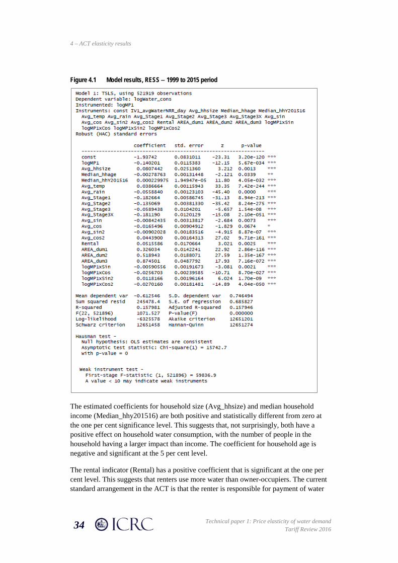
4 – 296BACT elasticity results
34 Technical paper 1: Price elasticity of water demand
Tariff Review 2016
Figure 4.1 Model results, RESS − 1999 to 2015 period
The estimated coefficients for household size (Avg_hhsize) and median household income (Median_hhy201516) are both positive and statistically different from zero at the one per cent significance level. This suggests that, not surprisingly, both have a positive effect on household water consumption, with the number of people in the household having a larger impact than income. The coefficient for household age is negative and significant at the 5 per cent level.
The rental indicator (Rental) has a positive coefficient that is significant at the one per cent level. This suggests that renters use more water than owner-occupiers. The current standard arrangement in the ACT is that the renter is responsible for payment of water

4 – 296BACT elasticity results
Technical paper 1: Price elasticity of water demand Tariff Review 2016 35
(and other services) consumption charges where the property is separately metered.64 This would suggest that renters face a similar marginal price signal to owner-occupiers. However, anecdotal evidence suggests that, particularly in the past, some landlords elected to pay water consumption charges, up to certain amount for example, to ensure that gardens are watered. This would of course dampen any price signals getting to the renter.
The block size dummies (AREA_dum1, AREA_dum2 and AREA_dum3) are all significant at the one per cent level and positive, as one would expect. The size of the coefficients also increases from the first to the third dummy as block size increases.65
The estimated coefficients for the maximum temperature (Avg_temp) and rain (Avg_rain) variables are both significant at the one per cent level and show the expected signs. Households use more water the greater the temperature and less water the higher the rainfall.
The water restrictions dummy variables are all negative, as one would expect, and statistically different from zero at the one per cent significance level. The size of coefficients of Avg_Stage1, Avg_Stage2 and Av_Stage3 reflect the incremental nature of the restrictions scheme. Stage 1 restrictions are responsible for the bulk of the water reduction, with Stages 2 and 3 incrementally reducing water use by smaller amounts. The Avg_Stage3X dummy coefficient of -0.179, is slightly less than the combined Stage 2 and 3 coefficients of -0.194. This seems to reflect the very small bounce-back in water consumption levels following the lifting of water restrictions in late 2010.
Since the impacts of water restrictions may be season-dependent, with lower impact in winter than in summer, in the model specification stage, the Commission included multiplicative interactions for restrictions dummies and the Fourier seasonality variables. These interactions were dropped in the preferred specification shown in Figure 4.1 as they did not significantly improve the AIC.
Three of the seasonal variables (Avg_sin, Avgsin2 and Avg_cos2) are significant at the one per cent level, with the fourth (Avg_cos) significant at the 5 per cent level.
The coefficients of the season and price interaction variables (logMP1xSin, logMP1xCos, logMP1xSin2 and logMP1xCos2) are all significant at the one per cent level. Figure 4.2 illustrates the impact of the seasonal variables on the central elasticity estimate. The elasticity estimate varies from a low of -0.11 to a high of -0.19 with the latter coinciding with the generally warmer months. This result is consistent with the findings of Renwick and Green (2000) and Dalhuisen et al. (2001) as discussed in section 2.4. This seasonal variation has implications when considering price
64 See http://www.tenantsact.org.au/FAQRetrieve.aspx?ID=36385. 65 500 to 1,000, 1,000 to 1,500 and greater than 1,500 square metres.

4 – 296BACT elasticity results
36 Technical paper 1: Price elasticity of water demand
Tariff Review 2016
adjustments as an alternative to quantitative water restrictions for reducing outdoor water use during the summer months.
Figure 4.2 Seasonal interaction with elasticity estimate, RESS − 1999 to 2015 period
4.2.2 Sub-periods
The statistical results for the 1999 to 2006 sub-period are shown in Figure 4.3 while those for 2006 to 2015 are shown in Figure 4.4.
-0.25
-0.20
-0.15
-0.10
-0.05
0.00
01/0
7/19
99
22/0
7/19
99
12/0
8/19
99
02/0
9/19
99
23/0
9/19
99
14/1
0/19
99
04/1
1/19
99
25/1
1/19
99
16/1
2/19
99
06/0
1/20
00
27/0
1/20
00
17/0
2/20
00
09/0
3/20
00
30/0
3/20
00
20/0
4/20
00
11/0
5/20
00
01/0
6/20
00
22/0
6/20
00

4 – 296BACT elasticity results
Technical paper 1: Price elasticity of water demand Tariff Review 2016 37
Figure 4.3 Model results, RESS − 1999 to 2006 sub-period
The key result to note when running the preferred model specification over the 1999 to 2006 sub-period is that the coefficient for the price variable of -0.31, which is significant at the one per cent level, implies a more elastic demand response to price than is the case over the entire period.66 In contrast, the results from the post-structural break sub-period suggest a less elastic demand response of -0.04 than over the entire 1999 to 2015 period. This estimate is also significant at the one per cent level.67
66 The Avg_Stage3 and Avg_Stage3X variables are excluded from this model run as all values are zero over this sub-period. 67 The Avg_Stage1 variable is excluded from this model run as all values are one over this sub-period. Avg_Stage2 was excluded in favour of Avg_Stage3.
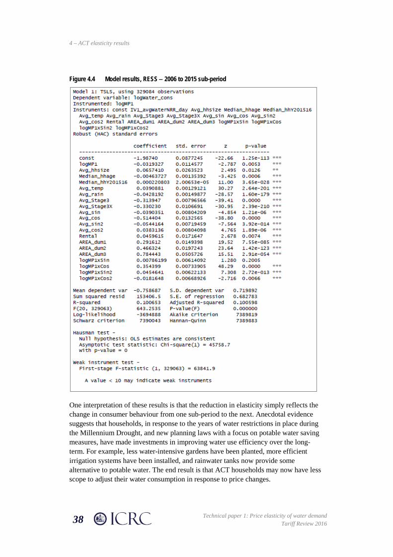
4 – 296BACT elasticity results
38 Technical paper 1: Price elasticity of water demand
Tariff Review 2016
Figure 4.4 Model results, RESS − 2006 to 2015 sub-period
One interpretation of these results is that the reduction in elasticity simply reflects the change in consumer behaviour from one sub-period to the next. Anecdotal evidence suggests that households, in response to the years of water restrictions in place during the Millennium Drought, and new planning laws with a focus on potable water saving measures, have made investments in improving water use efficiency over the long-term. For example, less water-intensive gardens have been planted, more efficient irrigation systems have been installed, and rainwater tanks now provide some alternative to potable water. The end result is that ACT households may now have less scope to adjust their water consumption in response to price changes.

4 – 296BACT elasticity results
Technical paper 1: Price elasticity of water demand Tariff Review 2016 39
4.3 Units and flats (ACP1) charge class
The ACP1 charge class captures the bulk of Icon Water residential customers living in units or flats rather than standalone houses.
There is a number of key differences between the RESS and ACP1 classes that has direct implications for the estimation of the price elasticity of demand of the latter class.
The first is that the ACP1 charge class differs from RESS by virtue of the fact that it is generally only the common property of the block of flats or units that is separately metered. This is reflected in the charging arrangements for ACP1 with tier water consumption allowance based on the number of units or flats in the complex. The owners’ corporation or equivalent receives the quarterly bill from Icon Water which is then shared among the residents. This means that, compared to the RESS class, price signals to the ACP1 charge class are likely to be somewhat muted.
The second is that the water use of the ACP1 class is likely to be less weather dependent than that of RESS as outdoor garden water use in the main will be restricted to the common property gardens. Similarly, ACP1 customers are likely to be less impacted by temporary water restrictions as these are primarily aimed at curbing outdoor water use.
Both of these differences are reflected in the statistical results for the preferred ACP1 model over the period 1999 to 2015 as shown in Figure 4.5.
The estimated coefficient for the price variable of -0.07, significant at the one per cent level, implies a much lower elasticity than that of -0.14 estimated for the RESS class. This could reflect the fact that unit and flat dwellers have less opportunity to adjust discretionary use in response to changes in price. The less elastic result may also be due to the lack of a strong price signal reaching individual customers.
The temperature and rain coefficients, although significant at the one per cent level, are smaller in size than those estimated for the RESS class. In addition, only Stage 1 restrictions made it into the preferred specification and the various seasonal and seasonal interaction variables are almost all not significant at the 10 per cent level.
The sub-period results for ACP1 show a similar pattern to that of RESS, with a more elastic response in the 1999 to 2006 sub-period (-0.46) followed by an elasticity response not significantly different from zero post the structural break.
4 – 296BACT elasticity results
40 Technical paper 1: Price elasticity of water demand
Tariff Review 2016
Figure 4.5 Model results, ACP1 − 1999 to 2015 period
A word of caution is required in relation to the interpretation of the ACP1 estimation results presented in this section because this charge class also includes a number of commercial common property arrangements. The water consumption behaviour between commercial tenancies and residential units and flats is unlikely to be the same.
4.4 Commercial (COMM) charge class
The COMM charge class captures the majority of Icon Water’s commercial customers, those that are separately metered and on one parcel of land.
As noted in section 2.2, water can be used in a number of different ways, which can potentially result in different demand functions for different uses. In particular, it is important to avoid pooling the quantity of water demanded across categories as this ‘imposes the restriction that the specifications are homogeneous, no matter what type

4 – 296BACT elasticity results
Technical paper 1: Price elasticity of water demand Tariff Review 2016 41
of use.’68 It is for this reason that the Commission has in this paper undertaken a separate estimation for the COMM charge class.
Notwithstanding this, it is important to note that the business units within COMM are likely to be heterogeneous in scale and nature of their business and that, unlike for the RESS class with its range of socio-economic variables, there are limited explanatory variables to measure those differences beyond block size.
For example, demand for water in the commercial sector is more likely to be a derived demand in the course of producing goods and services with cost minimisation or profit maximisation as the objective function. As such, it would be useful to at least have an indicator reflecting the industry category for each of the sample customers.
Given this heterogeneity issue, caution should be applied when interpreting the COMM results. The statistical results for the preferred COMM model over the period 1999 to 2015 are shown in Figure 4.6.
The key point to note from these results is that the estimated elasticity of -0.32, which is significant at the one per cent level, is much more elastic than the estimate for RESS over the same period.
The estimated coefficients for the maximum temperature (Avg_temp) and rain (Avg_rain) variables and show the expected signs, but only the latter is significant at any level.
The block size dummies (AREA_dum1, AREA_dum2 and AREA_dum3) have been adjusted from those applied in the RESS case to reflect the distribution of commercial block sizes.69 The larger two dummies are significant at the one per cent level and positive, as one would expect. The size of the coefficients also increases from the first to the third dummy as block size increases, as was the case for RESS.
The sub-period results for COMM show a similar pattern to that of RESS, with a slightly more elastic response in the 1999 to 2006 sub-period (-0.34) followed by an elasticity response not significantly different from zero post the structural break.
68 Espey, Espey and Shaw, 1997: 1370. 69 800 to 2,000, 2,000 to 5,000 and greater than 5,000 square metres.
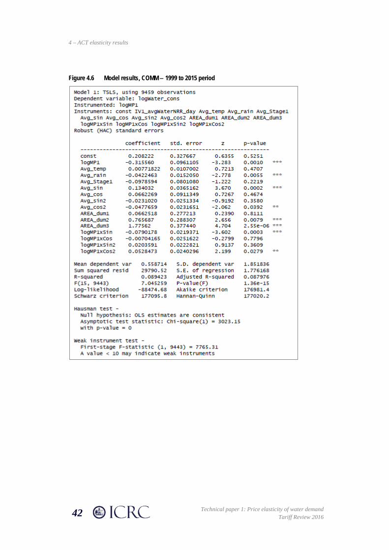
4 – 296BACT elasticity results
42 Technical paper 1: Price elasticity of water demand
Tariff Review 2016
Figure 4.6 Model results, COMM − 1999 to 2015 period

Technical paper 1: Price elasticity of water demand Tariff Review 2016 43
5 ConclusionWhile fuller consideration will await the tariff review draft report, some preliminary observations are made below.
This paper corroborates the view that the price elasticity of demand for residential water while not zero is relatively small.
The point estimate of -0.14 across the 1999 to 2015 period for the RESS charge class implies that a 10 per cent increase in the marginal price of water, which is the weighted average volumetric price of water in the preferred specification, would lead to a 1.4 per cent reduction in household water consumption on average.
Under the current ACT temporary water restrictions scheme, Stage 3 restrictions target a 35 per cent reduction in water use relative to permanent water conservation measures.70 Given the elasticity estimate above, to achieve this reduction in demand would require a 250 per cent increase in the average volumetric price. Applying the more elastic summer estimate of -0.19 implies a price increase in excess of 180 per cent to meet the water reduction objective. Furthermore, prices of this magnitude are well outside the data used for this analysis, and therefore the demand response would be uncertain.
This finding therefore mitigates against the use of price as a tool to manage water demand in the ACT. The finding that the residential price response is less elastic in the sub-period after the 2006 structural break than over the entire 1999 to 2015 period further supports this conclusion.
As noted in the introduction, Ramsey pricing involves deliberate and systematic price discrimination on the basis of elasticities of demand to allow the monopoly business to recover residual costs while minimising the deviations from optimal, that is based on marginal cost pricing, consumption patterns.
This paper found that, in general and bearing in mind the caveats around the estimates for COMM and ACP1, the demand response is the most price elastic for commercial customers and least elastic for units and flats customers, with residential customers in the middle. Should Ramsey pricing be contemplated, this would imply that units and flats customers, who are price inelastic, could be charged a higher price than the more price elastic commercial and residential customers. Alternatively, both residential and units and flats customers could pay a higher charge.
70 ACT Government, 2010: 3.

Technical paper 1: Price elasticity of water demand Tariff Review 2016 45
Appendix 1 Elasticity of demand definition
The responsiveness of demand for a good or service to a change in price is known as the price elasticity of demand. It can be formally defined as:
the ratio of the percentage change in quantity demanded divided by the percentage change in price that brought it about.71
The price elasticity of demand, η, is presented algebraically in equation A1.1:
𝜂𝜂 = Percentage change in quantity Percentage change in price
............ (A1.1)
The value of the price elasticity of demand ranges from minus infinity (∞) to zero, but, for comparison purposes, the absolute values are used. Figure A1.1 illustrates the range of elasticities for the standard downward-sloping demand curve. Demand is said to be elastic when η > 1, that is when the percentage change in the quantity demanded exceeds the percentage change in price. Conversely, demand is inelastic when η < 1 or when the percentage change in the quantity demanded is less than the percentage change in price.
Figure A1.1 Price elasticity of demand
Source: Adapted from Lipsey (1989).
The primary determinant of the price elasticity of demand is the availability of substitutes. Two goods are considered substitutes if the quantity demanded of one is positively related to the price of the other. Generally speaking, a good with close
71 Lipsey, 1989: 81.
Quantity
Price
Demand curve
η = ∞
η > 1 elastic demand
η = 1 unit elasticity
η = 0
η < 1 inelastic demand

Appendix 1Error! Reference source not found. – 341BElasticity of demand definition
46 Technical paper 1: Price elasticity of water demand
Tariff Review 2016
substitutes tends to have an elastic demand, while one with no close substitutes tends to have an inelastic demand. Butter is an example of the former, while diamonds are examples of the latter.
Price elasticity of demand can also have a short and long-run component. For example, a good with an inelastic demand in the short-run may have a long-run elastic demand as substitutes are developed over time. Taylor (1975) noted this issue in his seminal work on electricity demand.72
72 Taylor, 1975: 80.

Technical paper 1: Price elasticity of water demand Tariff Review 2016 47
Appendix 2 Semi-log model results This appendix presents the results of the semi-log specification of the preferred model specification discussed in Chapter 4. The results are shown in Figure A2.1.
As discussed earlier, the semi-log specification produces an elasticity of demand that varies with water consumption levels. Unlike the double-log form where the price elasticity of demand can be read directly off the price coefficient estimate, the semi-log case requires an additional calculation.
Following McNair (2006), the price elasticity of demand can be expressed as:
𝜂𝜂𝑝𝑝 =𝛿𝛿𝛿𝛿𝛿𝛿𝛿𝛿𝛿𝛿𝛿𝛿_𝑐𝑐𝑐𝑐𝑙𝑙𝑐𝑐
𝛿𝛿𝑀𝑀𝑃𝑃×
𝑀𝑀𝑃𝑃𝛿𝛿𝛿𝛿𝛿𝛿𝛿𝛿𝛿𝛿_𝑐𝑐𝑐𝑐𝑙𝑙𝑐𝑐
The structural demand equation can be written in the form:
𝛿𝛿𝛿𝛿𝛿𝛿𝛿𝛿𝛿𝛿𝑐𝑐𝑐𝑐𝑐𝑐𝑐𝑐 = 𝛿𝛿(𝛼𝛼+𝛽𝛽1𝑀𝑀𝑀𝑀+𝛽𝛽𝑥𝑥𝑋𝑋)
Using the chain rule:
𝛿𝛿𝛿𝛿𝛿𝛿𝛿𝛿𝛿𝛿𝛿𝛿_𝑐𝑐𝑐𝑐𝑙𝑙𝑐𝑐𝛿𝛿𝑀𝑀𝑃𝑃
= 𝛽𝛽1 × 𝛿𝛿𝛿𝛿𝛿𝛿𝛿𝛿𝛿𝛿_𝑐𝑐𝑐𝑐𝑙𝑙𝑐𝑐
The price elasticity of demand can then be expressed as:
𝜂𝜂𝑝𝑝 = 𝛽𝛽1 ×𝑀𝑀𝑃𝑃
Using the final equation above, and the marginal price coefficient shown in Figure 4.1, the price elasticity of demand can be calculated for a range of suburb categories. The results imply that demand is more elastic to changes in price at higher than lower prices. The semi-log results produce elasticities that are only slightly less than those generated by the preferred double-log specification.
Table A2.1 Semi-log price elasticity of demand results
Category MP1 Elasticity estimate All suburbs – mean 2.50 -0.107 − median 2.98 -0.127 Higher-income suburbs – mean 2.60 -0.111 − median 3.00 -0.128
Lower-income suburbs − mean 2.43 -0.104
− median 2.85 -0.122

Appendix 2 – 342BSemi-log model results
48 Technical paper 1: Price elasticity of water demand
Tariff Review 2016
Figure A2.1 Semi-log model results, RESS − 1999 to 2015 period

Technical paper 1: Price elasticity of water demand Tariff Review 2016 49
Abbreviations and acronyms 2SLS two stage least squares
ABS Australian Bureau of Statistics
ACP1 units and flats charge class
ACT Australian Capital Territory
AIC Akaike Information Criterion
BOM Bureau of Meteorology
COMM commercial charge class
Commission Independent Competition and Regulatory Commission
DCC discrete/continuous choice
GLS generalised least squares
HAC heteroscedasticity and autocorrelation consistent
ICRC Independent Competition and Regulatory Commission
ICRC Act Independent Competition and Regulatory Commission Act 1997 (ACT)
IV instrumental variables
kL kilolitre
MLE maximum likelihood estimation
PLS ordinary least squares
PWCM Permanent water conservation measures
RESS residential charge class
SQL structured query language
UNFT utilities network facilities tax
WAC Water Abstraction Charge

Technical paper 1: Price elasticity of water demand Tariff Review 2016 51
ReferencesACT Government 2010. "Utilities (Water Restrictions Scheme) Approval 2010 (No
1)." Canberra: ACT Legislative Assembly.
Arellano, M 2003. Panel data econometrics, Oxford University Press.
Baltagi, BH 2005. Econometric analysis of panel data, John Wiley & Sons, Ltd.
Barkatullah, N 2002. "OLS and Instrumental Variable Price Elasticity Estimates for Water in Mixed-Effect Models Under a Multipart Tariff Structure." London: London Economics.
Basman, R 1957. "A Generalized Classical Method of Linear Estimation of Coefficients in a Structural Equation." Econometrica. 25, 77-83.
Burtless, G and Hausman, JA 1978. "The Effect of Taxation on Labor Supply: Evaluating the Gary Negative Income Tax Experiment." Journal of Political Economy. 86, 1103-1130.
Cameron, CA and Trivedi, PK 2005. Microeconomics: Methods and applications Cambridge University Press.
Carter, DW and Milon, JW 2005. "Price Knowledge in Household Demand for Utility Services." Land Economics. 81, 265-283.
Dalhuisen, JM, Florax, RJ, De Groot, HL and Nijkamp, P 2001. "Price and income elasticities of residential water demand: Why empirical estimates differ." Amsterdam: Tinbergen Institute.
Dalhuisen, JM, Florax, RJ, de Groot, HL and Nijkamp, P 2003. "Price and Income Elasticities of Residential Water Demand: A Meta-Analysis." Land Economics. 79, 292-308.
Deller, SC, Chicoine, DL and Ramamurthy, G 1986. "Instrumental Variables Approach to Rural Water Service Demand*." Southern Economic Journal. 53, 333-346.
Epstein, RJ 1989. "The fall of OLS in structural estimation." Oxford Economic Papers. 41, 94-107.
Espey, M, Espey, J and Shaw, W 1997. "Price elasticity of residential demand for water: A meta analysis." Water Resources Research. 33, 1369-1374.
Goldberger, AS 1964. Econometric theory, John Wiley and Sons, New York.
Grafton, RQ, Kompas, T, To, H and Ward, M 2009. "Residential Water Consumption: A Cross Country Analysis." Canberra: Environmental Economics Research Hub

References
52 Technical paper 1: Price elasticity of water demand
Tariff Review 2016
Research Reports, Environmental Economics Research Hub, Crawford School of Public Policy, The Australian National University.
Grafton, RQ, Kompas, T and Ward, M 2011. "Estimates of Price Elasticities of Demand for Water in the ACT." Canberra: Sustainable Environment Group.
Graham, D and Scott, S 1997. "Price Elasticity and Sustainable Water Prices: Policy directions." Canberra: ACTEW Corporation.
Greene, WH 2012. Econometric analysis, New York, Prentice Hall.
Hansen, CB 2006. "Generalized Least Squares Inference in Panel and Multilevel Models with Serial Correlation and Fixed Effects." Journal of Econometrics. 140, 670-694.
Hausman, JA 1978. "Specification Tests in Econometrics." Econometrica. 46, 1251-1271.
Hausman, JA 1983. Stochastic Problems in the Simulation of Labor Supply. In: Feldstein, M (ed.) Behavioral Simulation Methods in Tax Policy Analysis. University of Chicago Press.
Howe, CW and Linaweaver, FJ 1967. "The impact of price on residential water demand and its relation to system design and price structure." Water Resources Research. 3, 13-32.
Hyndman, RJ 2010. "Forecasting with long seasonal periods." http://robjhyndman.com/hyndsight/longseasonality/.
ICRC 2004. "Final Report and Price Direction: Investigation into prices for water and wastewater services in the ACT." Canberra: Independent Competition and Regulatory Commission
ICRC 2008. Water and Wastewater Price Review: Final Report and Price Determination. Report 1 of 2008, Independent Competition and Regulatory Commission, Canberra ACT.
ICRC 2015a. "Issues Paper: Tariff Review 2016 - Regulated Water and Sewerage Services." Canberra: ICRC.
ICRC 2015b. "Water Demand Forecasting Final Technical Paper." Canberra: Independent Competition and Regulatory Commision.
Ito, K 2014. "How Do Consumers Respond to Marginal or Average Price? Evidence from Nonlinear Electricity Pricing " American Economic Review. 104, 537-63.
Lipsey, RG 1989. Positive Economics, London, George Weidenfield and Nicolson Ltd.

References
Technical paper 1: Price elasticity of water demand Tariff Review 2016 53
McNair, BJ 2006. "Managing Urban Water Supply Shortages." Canberra: Australian National University.
Megdal, SB 1987. "The Econometrics of Piecewise-Linear Budget Constraints: A Monte Carlo Study." Journal of Business and Economic Statistics. 5, 243-248.
Moffitt, R 1986. "The Econometrics of Piecewise-Linear Budget Constraints: A Survey and Exposition of the Maximum Likelihood Method." Journal of Business and Economic Statistics. 4, 317-328.
Moffitt, R 1990. "The Econometrics of Kinked Budget Constraints." The Journal of Economic Perspectives. 4, 119-139.
Nieswiadomy, ML 1992. "Estimating urban residential water demand: Effects of price structure, conservation, and education." Water Resources Research. 28, 609–615.
Nieswiadomy, ML and Molina, DJ 1989. "Comparing Residential Water Demand Estimates under Decreasing and Increasing Block Rates Using Household Data " Land Economics. 65, 280-289.
Nieswiadomy, ML and Molina, DJ 1991. "A Note on Price Perception in Water Demand Models." Land Economics. 67, 352-359.
Nordin, JA 1976. "A proposed modification of Taylor's demand analysis: Comment." The Bell Journal of Economics. 7, 719-721.
Olmstead, SM 2009. "Reduced-Form versus Structural Models of Water Demand under Nonlinear Prices." Journal of Business and Economic Statistics. 27, 84-94.
Reiss, PC and Wolak, FA 2007. Structural econometric modeling: Rationales and examples from industrial organization, Oxford University Press.
Renwick, ME and Green, RD 2000. "Do Residential Water Demand Side Management Policies Measure Up? An Analysis of Eight California Water Agencies." Journal of Environmental Economics and Management. 40, 37-55.
Sargan, J 1958. "The Estimation of Economic Relationships Using Instrumental Variables." Econometrica. 26, 393-415.
Shin, J-S 1985. "Perception of price when price information is costly: evidence from residential electricity demand." Review of Economics and Statistics. 67, 591–598.
Taylor, LD 1975. "The Demand for Electricity: A Survey." The Bell Journal of Economics. 6, 74-110.

References
54 Technical paper 1: Price elasticity of water demand
Tariff Review 2016
Theil, H 1992. Estimation and simultaneous correlation in complete equation systems. Henri Theil’s Contributions to Economics and Econometrics. Central Planning Bureau, The Hague.
Wooldridge, JM 2002. Econometric Analysis of Cross Section and Panel Data, Cambridge Massachusetts, The MIT Press.
Worthington, AC and Hoffman, M 2008. "An empirical survey of residential water demand modelling." Journal of Economic Surveys. 22, 842-871.