Technical Note PR-TN 2014/00384 · The receiver of such a report must ensure ... Technical Note:...

Technical Note PR-TN 2014/00384

Issued: 08/2014

Xi Yang, Xi Long, Reinder Haakma, Ronald M. Aarts

Philips Research Europe

Company Confidential until 2017-08

Company Confidential reports are issued personally. The receiver of such a report must ensure

that this information is not shared with anyone unauthorized, inside or outside Philips. Access by

others has to be approved individually by the group leader of the first author.

Koninklijke Philips N.V. 2014

PR-TN 2014/00384 Company Confidential until 2017-08

ii


Authors’ address Xi Yang HTC34-5.012 [email protected] Xi Long HTC34-5.013 [email protected] Reinder Haakma HTC34-5.001 [email protected] Ronald M. Aarts HTC34-5.001 [email protected]

© KONINKLIJKE PHILIPS NV 2014 All rights reserved. Reproduction or dissemination in whole or in part is prohibited without the prior written consent of the copyright holder .

mailto:[email protected]




Company Confidential until 2017-08 PR-TN 2014/00384


iii

Title: Classification and Exploration of Sleep Stages with Cardiorespiratory Signals Based on Autoregressive Models

Author(s): X. Yang, X. Long, R. Haakma, R. M. Aarts

Reviewer(s): X. Long

Technical Note:

PR-TN 2014/00384

Additional Numbers:

Subcategory:

Project: Sleep and stress monitoring for WeST

Customer:

Keywords: Sleep, classification, analysis, clustering, micro-stage

Abstract:

This report comprises two goals. The first goal is to investigate to what extent cardiorespiratory activity can provide information about sleep stages; the second goal is the analysis of overnight sleep with respect to finer micro-stages compared with the current definition of sleep stages. To extract information regarding sleep stages from respiratory effort and cardiac activity, we use autoregressive- (AR-) based models. The use of cardiorespiratory signals is because they can be acquired unobtrusively. The first part of this thesis focuses on automatic sleep stage classification by incorporating a total of 9 new features extracted with AR models. To examine the performance of sleep stage classifica-tion, we use two classification algorithms including linear discriminant (LD) and hidden Markov model with unsupervised Gaussian mixture model (GMM-HMM). The second part is to explore possible micro-stages, which is done by clustering a total of 23 AR features and com-puting the between-subject agreement based on the clustering results. For sleep stage classification, results show that the new AR features are discriminative in distinguishing between different sleep stages. Adding AR features to an existing feature set can improve the classifi-cation performance. In addition, we found that the GMMHMM classifier performed better than the LD classifier when AR features are used. For the second part, some micro-stages are found, but some of the micro stages cannot be clearly explained, which suggest that further study is needed.


iv


Conclusions: An exploration of sleep stages based on cardiorespiratory signals is presented in this report. We use AR models to extract physiological information from respiratory effort and ECG signals. The AR features show discriminative power among existing cardiorespiratory features, and give improvement in classification performances. Comparing LD and GMM-HMM classifiers, the performance of GMM-HMM is generally higher than the performance of LD when AR features are used. From this observation we speculate that AR features contain the information of sleep stage transitions. Apart from sleep staging, much emphasis has been put on proving that the R&K rules do not fully describe the sleep stages. The preliminary results from the exploration of micro-stages show that the clusters can be seen as microstages of the sleep structure, the meaning of some clusters can be explained, but for some clusters, their meanings are still unclear. This suggests that more investigations need to be done on exploring the physiological meaning of each cluster.



v

Contents

1. Introduction .......................................................................................................................... 7

1.1. Objective ...................................................................................................................... 7

1.2. Project Scope .............................................................................................................. 8

1.3. Solution approach........................................................................................................ 9

1.4. Possible applications ................................................................................................... 9

1.5. Intended audience ..................................................................................................... 10

2. Background ........................................................................................................................ 11

2.1. Physiology of sleep.................................................................................................... 11

2.2. Cardiorespiratory signal acquisition .......................................................................... 12

2.3. Automatic sleep analysis ........................................................................................... 13

2.3.1. Related work ................................................................................................. 13

2.3.2. Sleep stage classification framework ........................................................... 14

2.4. Exploration of micro-stages ....................................................................................... 14

3. Data ..................................................................................................................................... 16

4. Sleep stage classification based on Autoregressive model ......................................... 17

4.1. Autoregressive model ................................................................................................ 17

4.1.1. Uni-variate AR models ..................................................................................... 17

4.1.2. Multi-variate AR models .................................................................................. 18

4.2. Gaussian Mixture Model ............................................................................................ 20

4.2.1. Model contruction .......................................................................................... 20

4.2.2. Evaluation criteria ........................................................................................... 21

4.3. Feature extraction...................................................................................................... 23

4.3.1. Existing features: ............................................................................................. 23

4.3.2. AR features: .................................................................................................... 23

4.4. Classification ............................................................................................................. 24

4.4.1. Linear Discriminant ......................................................................................... 24

4.4.2. GMM-HMM classifier ...................................................................................... 24

4.4.3. Evaluation criteria ........................................................................................... 26

5. Exploration of micro-stages ............................................................................................. 27

5.1. Clustering .................................................................................................................. 27

5.2. Between-subject agreement ...................................................................................... 27

5.3. Computation of Between-subject agreement ............................................................ 28

5.3.1. AIC ................................................................................................................ 28

5.3.2. Minimum Mahalanobis distance ................................................................... 28

6. Results and Discussion .................................................................................................... 30


vi


6.1. Part I: sleep stage classification results .................................................................... 30

6.1.1. AR feature normality test results: ................................................................. 30

6.1.2. AR feature selection ..................................................................................... 30

6.1.3. AR feature evaluation ................................................................................... 31

6.1.4. Sleep stage classification performance ........................................................ 32

6.2. Part II: Results from the Exploration of Micro-stages ................................................ 33

6.2.1. AR feature selection for clustering ............................................................... 33

6.2.2. Between-subject agreement ......................................................................... 34

7. Conclusions ....................................................................................................................... 37

8. Recommendations ............................................................................................................. 37

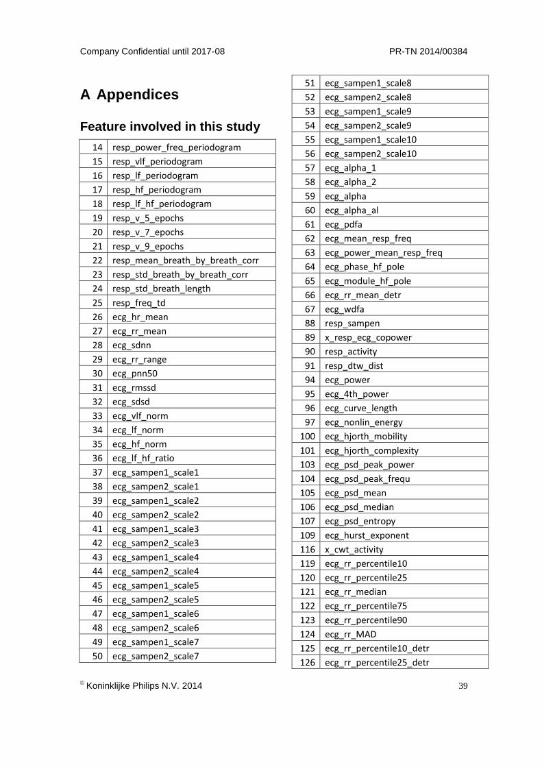
A Appendices ........................................................................................................................ 38

Feature involved in this study .................................................................................................. 38

References ................................................................................................................................. 40



7

1. Introduction

Sleep is a complex mixture of physiologic and behavioral processes. By means of visually in-specting brain wave (Electroencephalography), eye movements (Electrooculography), muscle activity (Electromyography) and heart rhythm (Electrocardiography), sleep technicians distin-guish sleep to five or six stages according to the traditional Rechtschaffen & Kales (R&K) rules[1] or the more recent American Academy of Sleep Medicine(AASM) rules[2]. These so called gold standard of clinical sleep medicine (technician-attended laboratory based Polysomnography) provides accurate and detailed physiology measurements during sleep. However, it has several drawbacks, particularly the expensive diagnostic equipment and sleep lab; the obtrusive meas-urement due to the change of sleep environment and the large variance between different sleep experts. Moreover, many researchers have discovered that the Polysomnography (PSG) measurement contains more information than we already knew. For instance, there are at least two different wakefulness stages exist, or S2 is a heterogeneous stage which should be sub-divided. Therefore, further investigation on the possible new definition of sleep profile is sug-gested by the current state of arts in the area of sleep analysis.

1.1. Objective

Main goal of this study is to investigate to what extent human sleep cardiorespiratory signals based on Autoregressive model (AR) can provide information about sleep stages. First step is to show that, as a cardiorespiratory feature, AR coefficient vectors carry information that is need-ed to distinguish different R&K sleep stages. Secondly, by applying different classification tasks, some research questions can be answered. For example, whether AR features could add value to the classification performance? AR features have good performace on which specific classifi-cation task? The focus of the sleep staging performance was on examining whether the sleep information is carried by AR features, rather than improving the kappa[3] value of classification performance.

Once enough evidence can support the hypothesis that AR coefficient vectors can be used as a feature, which means they are able to describe the characteristics of the sleep cardiorespir-atory behavior, a further investigation will be on the topic of finding whether there is temporal information hidden in the AR features. The topic of sleep staging using cardiorespiratory signals is not new, but those studies considered that sleep stages over night are independent and did not take the inter connections between sleep stage transitions into account. By comparing the classification performance of Linear Discriminant (LD) classifier and Hidden Markov Model (HMM) classifier, we hope to see that the AR features favor the HMM over LD, because of its well-known ability in temporal pattern recognition.

Unsupervised Gaussian Mixture Model (GMM) is used to generate observation sequences for HMM classifier. The last part of this study was to explore the behavior of the Gaussian kernels resulting from clustering the AR coefficients. We wish to find out that the signals rec-orded from PSG measurement contains more information than we already knew, and the hu-man sleep structure can be described in a finer way.


8


1.2. Project Scope

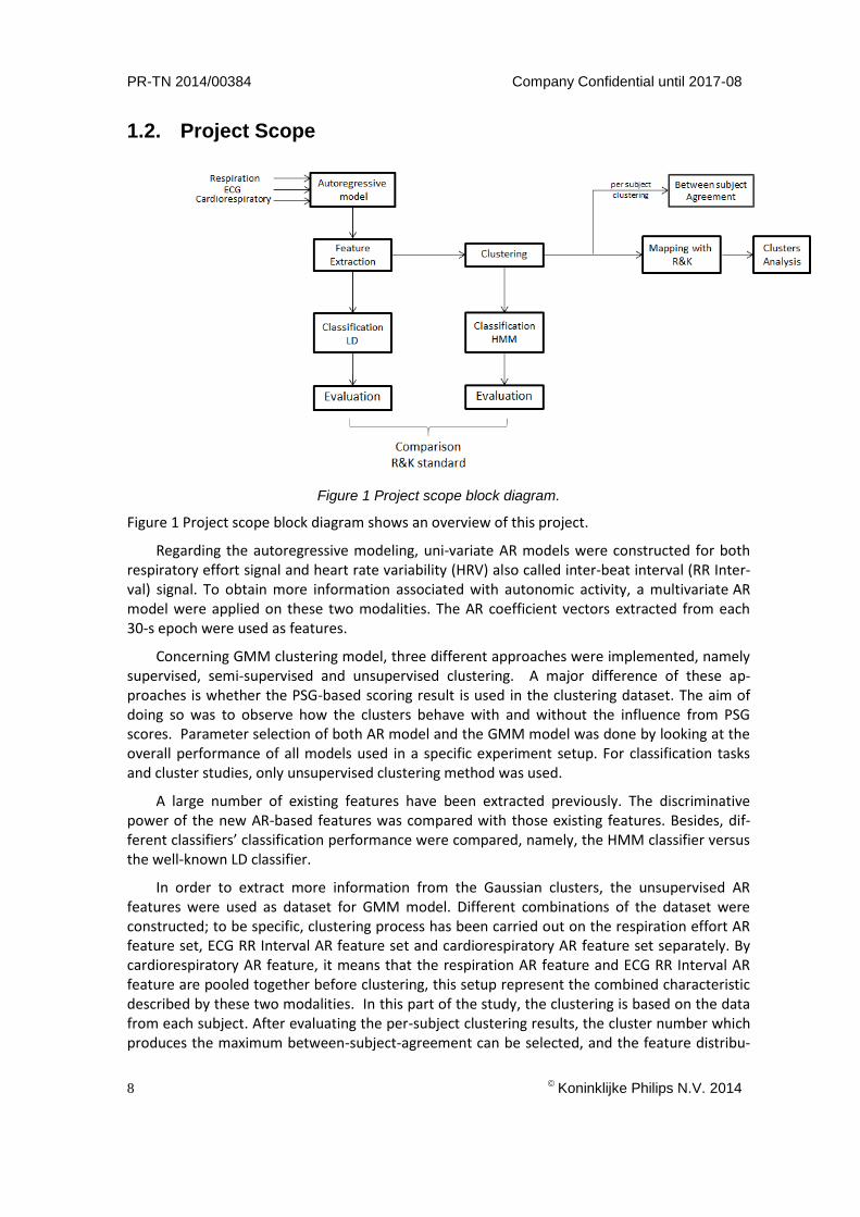
Figure 1 Project scope block diagram.

Figure 1 Project scope block diagram shows an overview of this project.

Regarding the autoregressive modeling, uni-variate AR models were constructed for both respiratory effort signal and heart rate variability (HRV) also called inter-beat interval (RR Inter-val) signal. To obtain more information associated with autonomic activity, a multivariate AR model were applied on these two modalities. The AR coefficient vectors extracted from each 30-s epoch were used as features.

Concerning GMM clustering model, three different approaches were implemented, namely supervised, semi-supervised and unsupervised clustering. A major difference of these ap-proaches is whether the PSG-based scoring result is used in the clustering dataset. The aim of doing so was to observe how the clusters behave with and without the influence from PSG scores. Parameter selection of both AR model and the GMM model was done by looking at the overall performance of all models used in a specific experiment setup. For classification tasks and cluster studies, only unsupervised clustering method was used.

A large number of existing features have been extracted previously. The discriminative power of the new AR-based features was compared with those existing features. Besides, dif-ferent classifiers’ classification performance were compared, namely, the HMM classifier versus the well-known LD classifier.

In order to extract more information from the Gaussian clusters, the unsupervised AR features were used as dataset for GMM model. Different combinations of the dataset were constructed; to be specific, clustering process has been carried out on the respiration effort AR feature set, ECG RR Interval AR feature set and cardiorespiratory AR feature set separately. By cardiorespiratory AR feature, it means that the respiration AR feature and ECG RR Interval AR feature are pooled together before clustering, this setup represent the combined characteristic described by these two modalities. In this part of the study, the clustering is based on the data from each subject. After evaluating the per-subject clustering results, the cluster number which produces the maximum between-subject-agreement can be selected, and the feature distribu-



9

tion of these clusters can be further analyzed.

In order to find out the physiology meaning of the clusters, the mapping between clusters and R&K stages were first studied. To find out the connection between the clusters and the physiology activities happened during sleep, the distribution of the clusters was analyzed.

1.3. Solution approach

A single-night PSG recording of 82 subjects were used as dataset. To estimate how a classifier will perform in practice, the training and validation process is performed using 10-fold cross-validation technique. The classification performance is assessed by computing the Cohens kappa coefficient of agreement value (κ). This criterion is used because it does not influence by the imbalanced class distribution of sleep stages, therefore it won’t produce a biased estimation as those which give judgments only depend on the right wrong percentage.

The AR features’ discriminative power were examined with respect to different classes. ASMD value and ANOVA-F score are computed and ranked with other features. ASMD is to calculate the discriminative power between two classes, where ANOVA-F score is for multi classes. For a specific classification task, the feature set selection was done by using the auto-matic search method Correlation Feature Selection with Forward Search algorithm (CFS-FS)[4]. This method searches the feature which is highly correlated with the class yet least correlated with each other.

Chapter 2 gives an overview on the prior research of sleep staging. The classification framework and classifiers used by this study are explained in detail. Chapter 3 describes how the AR model and GMM model are constructed and tuned. The evaluation result for AR features and their classification performance are also stated. In Chapter 4, details on the cluster studies are explained. Finally, the conclusion for this study and discussion for the future work are de-scribed in Chapter 5.

1.4. Possible applications

The ultimate goal of automatic sleep detection is to replace the costly equipment of PSG record-ing together with its tedious manual scoring process. At the same time, it gives enormous opportunities for autonomous unobtrusive sleep monitoring system. The purpose of classifica-tions can be various; each implicates different real world applications. For example, REM/All classification can also be seen as REM sleep detection, which is useful for the study of early brain development of infants; Sleep/Wake classification can be used for analyzing people’s sleep quality; while deep sleep detection is critical for the study of body recovery and memory consolidation.

One other main goal of this study is to explore the existence of micro-stage. Since this field of study is very new, the possible application is still unclear. However, we have good motivation to look into this study, because criticism of traditional sleep staging already existed since the beginning of 21 century, sleep researchers call for breakthrough of sleep analysis. But still, research has been done in this topic are only first step towards demonstrating potential clinical use of the new concept.


10


1.5. Intended audience

This report is intended for readers with an academic background and familiarity with statistics. Basic knowledge of machine learning and sleep research are recommended.



11

2. Background

2.1. Physiology of sleep

Sleep cannot be seen as a simple monolithic state. On the contrary, it is a complex process, which often contains cyclic states. Initially, two states within sleep have been defined based on a constellation of physiologic parameters. They are Rapid Eye Movement (REM) and Non Rapid Eye movement (NREM).

REM: EEG is desynchronized, muscles are atonic, and dreaming is typically presented;

NREM: signature patterns of EEG such as sleep spindles, k-complexes and slow waves.

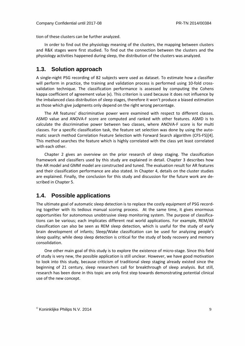
In R&K standard, NREM sleep is further subdivided into four stages (S1, S2, S3 and S4). In AASM standard, NREM is subdivided into three stages (N1, N2 and N3, where N1 and N2 are the same with S1 and S2, N3 is the combination of S3 and S4). A depiction of sleep characteristics is shown in Figure 2 Adepiction of brain activity during sleep.

Figure 2 Adepiction of brain activity during sleep.

S1: describes the transition from wake state into drowsy sleep. Conscious awareness of

the environment decreases, the subject begins to lose some of its muscle tone. Theta

waves (4 - 7Hz) become visible in the EEG whereas during relaxed wakefulness higher

frequency alpha waves (8 - 13Hz) are generated by the brain.

S2: involves so-called sleep spindles (11 - 16Hz) and K-complexes - both of which are ar-ticulate irregularities in the brain wave pattern. Conscious awareness completely van-ishes.

S3 & S4: (slow wave sleep) is scored if at least 20% delta waves (large amplitude figures with a frequency range of 0.5 - 2Hz) are present in the EEG. Sleepwalking, sleep-talking or other parasomnias are typically encountered in the S3 and S4 stages.


12


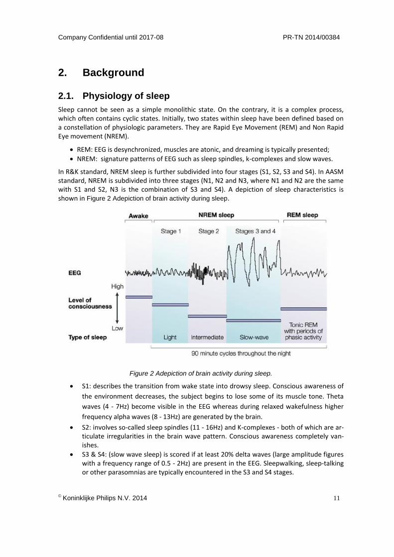
Objective sleep analysis is conventionally done with overnight Polysomnography (PSG) record-ings (see Figure 3 Polysomnography recording). It records the physiological changes occur during people’s sleep, which include brain wave (Electroencephalography), eye movements (Electrooculography), muscle activity (Electromyography) and heart rhythm (Electrocardiog-raphy). In the scoring process, experienced sleep technicians will visually inspect the PSG and give the sleep scoring results. An overnight PSG recording is typically divided into 30-s epochs, where each epoch can be classified into wake, REM sleep, or one of the NREM sleep stages (S1, S2, S3 and S4) according to the R&K rules. A healthy night of sleep can last between 7 to 9 hours; therefore a fully annotated night has approximately 840 to 1080 epochs.

Figure 3 Polysomnography recording

2.2. Cardiorespiratory signal acquisition

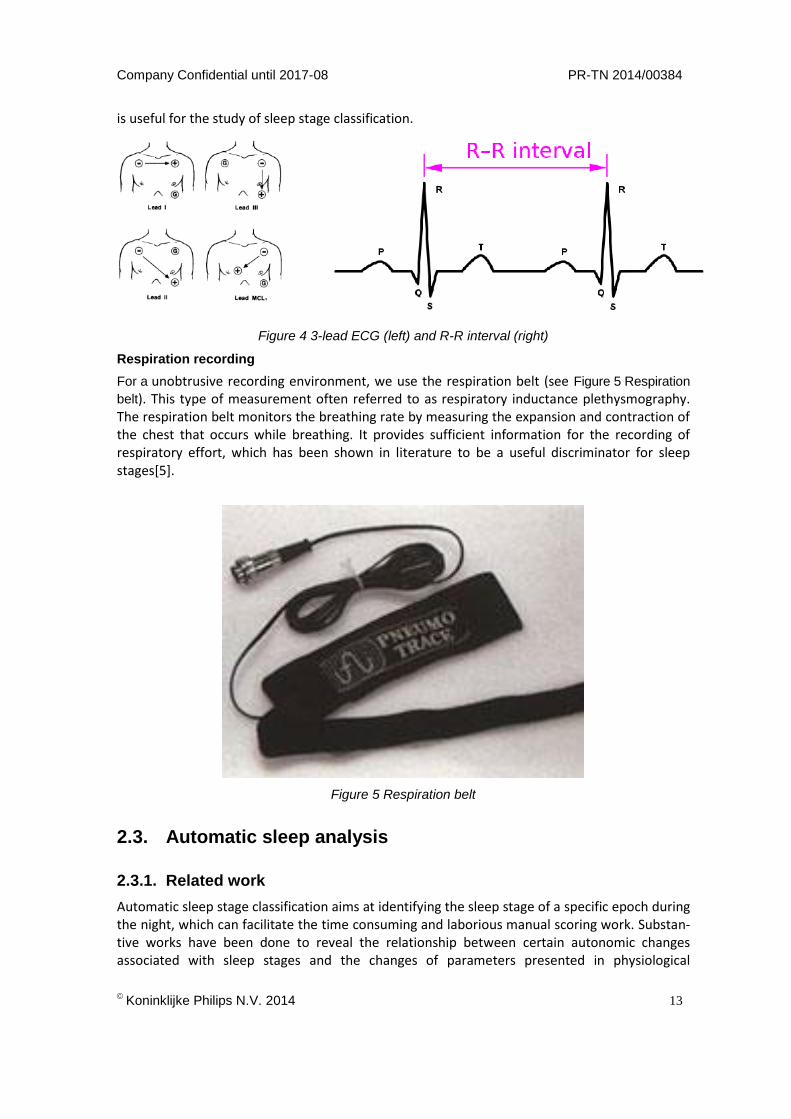
Among the five body function signals recorded in PSG, Cardiorespiratory signals can be collected unobtrusively or even with non-contact sensors. These setups can provide a subject with more natural environment, which has less interruption to their normal sleep. In the following para-graph, the acquisition process is briefly introduced. ECG ECG is used to measure the heart’s electrical conduction system. It picks up electrical impulses generated by the polarization and depolarization of cardiac tissue and translates into a wave-form. Different types of ECGs are referred by the number of leads that are used in the record-ing, for example 3-lead, 5-lead, or 12-lead ECGs. In this study, a 3-lead ECG is used to measure and derive the ECG signal, where two of the electrodes form the lead (positive and negative poles), the third considered a 'ground' connection (G). With the exception of the modified chest lead (MCL), all leads use the same electrodes or sensor placement. Limb lead II is the most common monitoring lead configuration, because it produces the largest positive R wave, which



13

is useful for the study of sleep stage classification.

Figure 4 3-lead ECG (left) and R-R interval (right)

Respiration recording

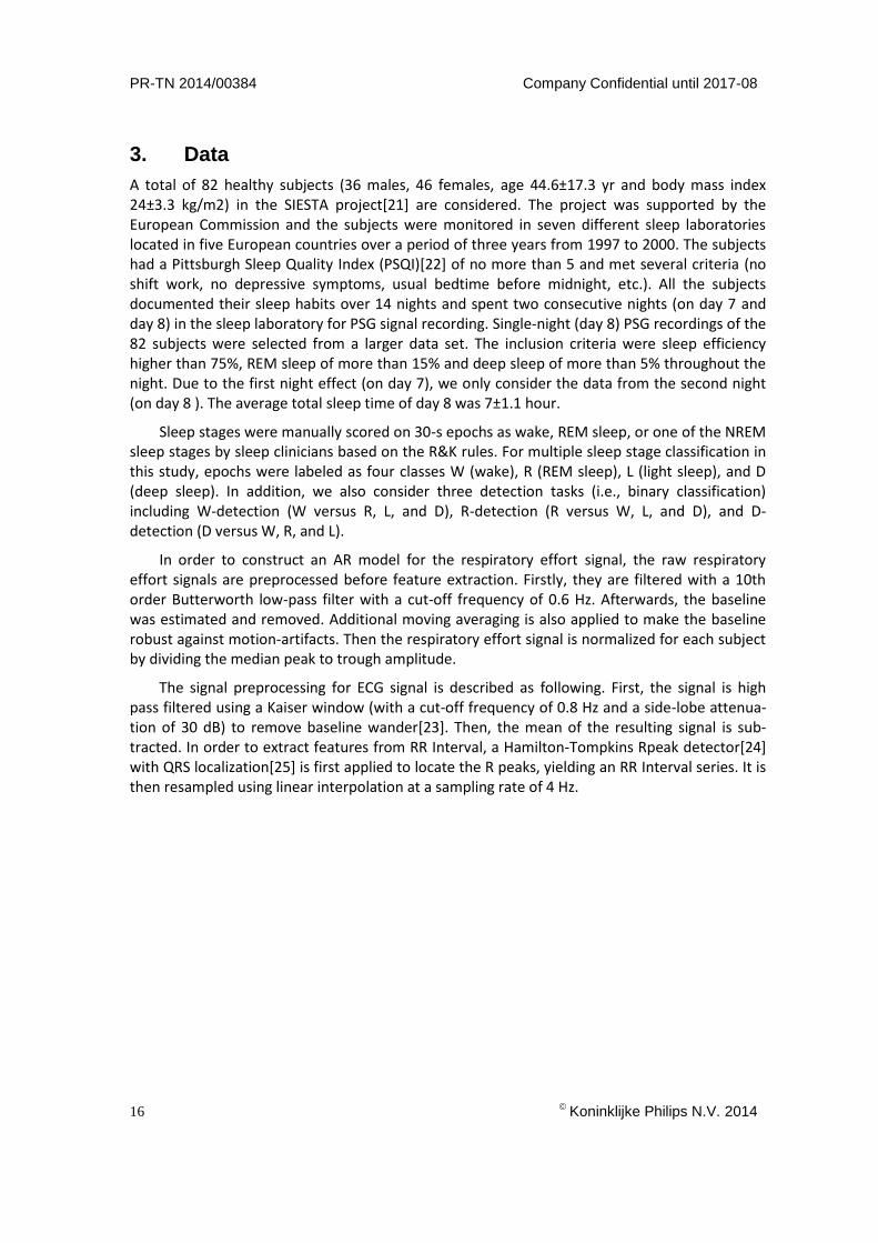
For a unobtrusive recording environment, we use the respiration belt (see Figure 5 Respiration

belt). This type of measurement often referred to as respiratory inductance plethysmography. The respiration belt monitors the breathing rate by measuring the expansion and contraction of the chest that occurs while breathing. It provides sufficient information for the recording of respiratory effort, which has been shown in literature to be a useful discriminator for sleep stages[5].

Figure 5 Respiration belt

2.3. Automatic sleep analysis

2.3.1. Related work

Automatic sleep stage classification aims at identifying the sleep stage of a specific epoch during the night, which can facilitate the time consuming and laborious manual scoring work. Substan-tive works have been done to reveal the relationship between certain autonomic changes associated with sleep stages and the changes of parameters presented in physiological


14


activity[6]–[8]. These parameters are usually called ’features’ for epoch-by-epoch classification of sleep stages. For example, a typical classification task can be identifying whether a certain epoch belongs to sleep or wake stage[9].

Cardiorespiratory-based automatic sleep stage classification has been increasingly studied in recent years [5], [10]–[12]. This is because among the PSG recordings, cardiorespiratory signals, can be collected unobtrusively[11], [12] or even with non-contact devices. Such device can be a wrist-worn watch[13], near-infrared camera[14], acoustic sensors[15], and respiratory inductance plethysmography (RIP) sensor[16]. These setups can provide a subject with more natural environment, which has less interruption to their normal sleep pattern.

2.3.2. Sleep stage classification framework

This section gives a brief overview on the classification process. A block diagram of the classification process is shown in Figure 6 Automatic sleep stage classification process. There are three main steps:

1. Extracting relevant information from the sensor recording. The raw sensor data does not always give good distinction between different sleep stages. Characteristics need to be extracted from the recordings which better describes the differences between sleep stages. Such a characteristic is referred to as a feature. The computation of these features from the original sensor recordings is called feature extraction. A most relevant feature set is selected acorrding to certain criterion to meet the classification requirements.

2. Training the classifier. The classifier is tuned to the selected feature set and annotation, such that the classifier can correctly classify the validation data set.

3. Validating the classification performance. The training and validation of the classifier is performed using separate sets of subjects in order to get a more reliable estimation of the classification performance. The training set has annotation as the training knowledge, and the predicted annotation is compared with the vilidation annotation.

2.4. Exploration of micro-stages

Strong criticism of traditional sleep staging exists in sleep research. Schulz[17] criticized that the standard sleep staging was appropriate as long as sleep physiological signals were recorded in the analog mode as curves on paper, whereas this staging may be insufficient for digitally rec-orded and stored sleep data. Himanen and Hasan[18] also argued that the R&K rule of sleep process has insufficient number of stages, and ignorance of physiological parameters such as autonomous nervous system activity. Sleep researchers call for the alternatives of sleep analysis which can detach from the brittle stages, and is not depending only on what can be visually seen in the signal. Instead of visual sleep scoring, more researches have been conducted to extract information from physiological signals[5], [10], [19], [20].



15

Figure 6 Automatic sleep stage classification process


16


3. Data

A total of 82 healthy subjects (36 males, 46 females, age 44.6±17.3 yr and body mass index 24±3.3 kg/m2) in the SIESTA project[21] are considered. The project was supported by the European Commission and the subjects were monitored in seven different sleep laboratories located in five European countries over a period of three years from 1997 to 2000. The subjects had a Pittsburgh Sleep Quality Index (PSQI)[22] of no more than 5 and met several criteria (no shift work, no depressive symptoms, usual bedtime before midnight, etc.). All the subjects documented their sleep habits over 14 nights and spent two consecutive nights (on day 7 and day 8) in the sleep laboratory for PSG signal recording. Single-night (day 8) PSG recordings of the 82 subjects were selected from a larger data set. The inclusion criteria were sleep efficiency higher than 75%, REM sleep of more than 15% and deep sleep of more than 5% throughout the night. Due to the first night effect (on day 7), we only consider the data from the second night (on day 8 ). The average total sleep time of day 8 was 7±1.1 hour.

Sleep stages were manually scored on 30-s epochs as wake, REM sleep, or one of the NREM sleep stages by sleep clinicians based on the R&K rules. For multiple sleep stage classification in this study, epochs were labeled as four classes W (wake), R (REM sleep), L (light sleep), and D (deep sleep). In addition, we also consider three detection tasks (i.e., binary classification) including W-detection (W versus R, L, and D), R-detection (R versus W, L, and D), and D-detection (D versus W, R, and L).

In order to construct an AR model for the respiratory effort signal, the raw respiratory effort signals are preprocessed before feature extraction. Firstly, they are filtered with a 10th order Butterworth low-pass filter with a cut-off frequency of 0.6 Hz. Afterwards, the baseline was estimated and removed. Additional moving averaging is also applied to make the baseline robust against motion-artifacts. Then the respiratory effort signal is normalized for each subject by dividing the median peak to trough amplitude.

The signal preprocessing for ECG signal is described as following. First, the signal is high pass filtered using a Kaiser window (with a cut-off frequency of 0.8 Hz and a side-lobe attenua-tion of 30 dB) to remove baseline wander[23]. Then, the mean of the resulting signal is sub-tracted. In order to extract features from RR Interval, a Hamilton-Tompkins Rpeak detector[24] with QRS localization[25] is first applied to locate the R peaks, yielding an RR Interval series. It is then resampled using linear interpolation at a sampling rate of 4 Hz.



17

……

epoch 1 epoch 2 epoch 3 epoch n

4. Sleep stage classification based on Autoregressive model

Many researchers have used features which are coefficients obtained by fitting intervals of time varying processes with an AR model[26]. Roberts et al.[19] worked with features which are 10-dimensional parameters obtained by fitting 1 second interval of EEG data with AR model. Each AR model is linked to a frequency distribution of the data, and the AR coefficients can be interpreted as a way of describing the frequency spectrum for the given interval[27]. Dorffner et al.[20] used AR models of EEG data to construct a probabilistic sleep model (PSM). In the PSM, a Gaussian mixture model (GMM)[28] was used to describe the space of AR coefficients in terms of Gaussian clusters, which were interpolated as micro-stages of sleep structure.

4.1. Autoregressive model

An autoregressive (AR) model is a statistical representation of a time-varying process; it fits a current data point to a linear function based on previous data points, such that

𝑋𝑡 = ∑ 𝜑𝑖𝑋𝑡−𝑖 + 휀𝑡 = 𝜑1𝑋𝑡−1 + ⋯ + 𝜑𝑖𝑋𝑡−𝑖 + 휀𝑡,𝑝𝑖=1 Equation 1

where 𝑋𝑡 is the data series under investigation, 𝑝 is the AR order which is generally much less

than the length of the series, 𝑋𝑡−𝑖 is the 𝑖𝑡ℎ data point before 𝑋𝑡, and 𝜑𝑖 is the corresponding AR coefficients. The noise εt is assumed to be Gaussian white noise. The current data point of the series is estimated by a linear weighted sum of previous 𝑖 terms in the series. With enough elements regressed, an AR model can fit an approximation to most stationary time series to a good precision. Here an AR model is fitted for each 30-s interval of respiration effort signal, or RR Interval signal.

4.1.1. Uni-variate AR models

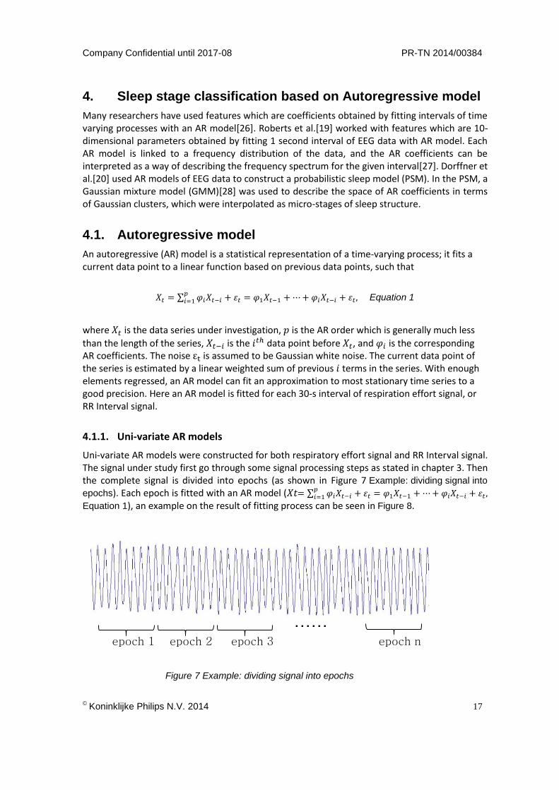
Uni-variate AR models were constructed for both respiratory effort signal and RR Interval signal. The signal under study first go through some signal processing steps as stated in chapter 3. Then the complete signal is divided into epochs (as shown in Figure 7 Example: dividing signal into

epochs). Each epoch is fitted with an AR model (𝑋𝑡= ∑ 𝜑𝑖𝑋𝑡−𝑖 + 휀𝑡 = 𝜑1𝑋𝑡−1 + ⋯ + 𝜑𝑖𝑋𝑡−𝑖 + 휀𝑡 ,𝑝𝑖=1

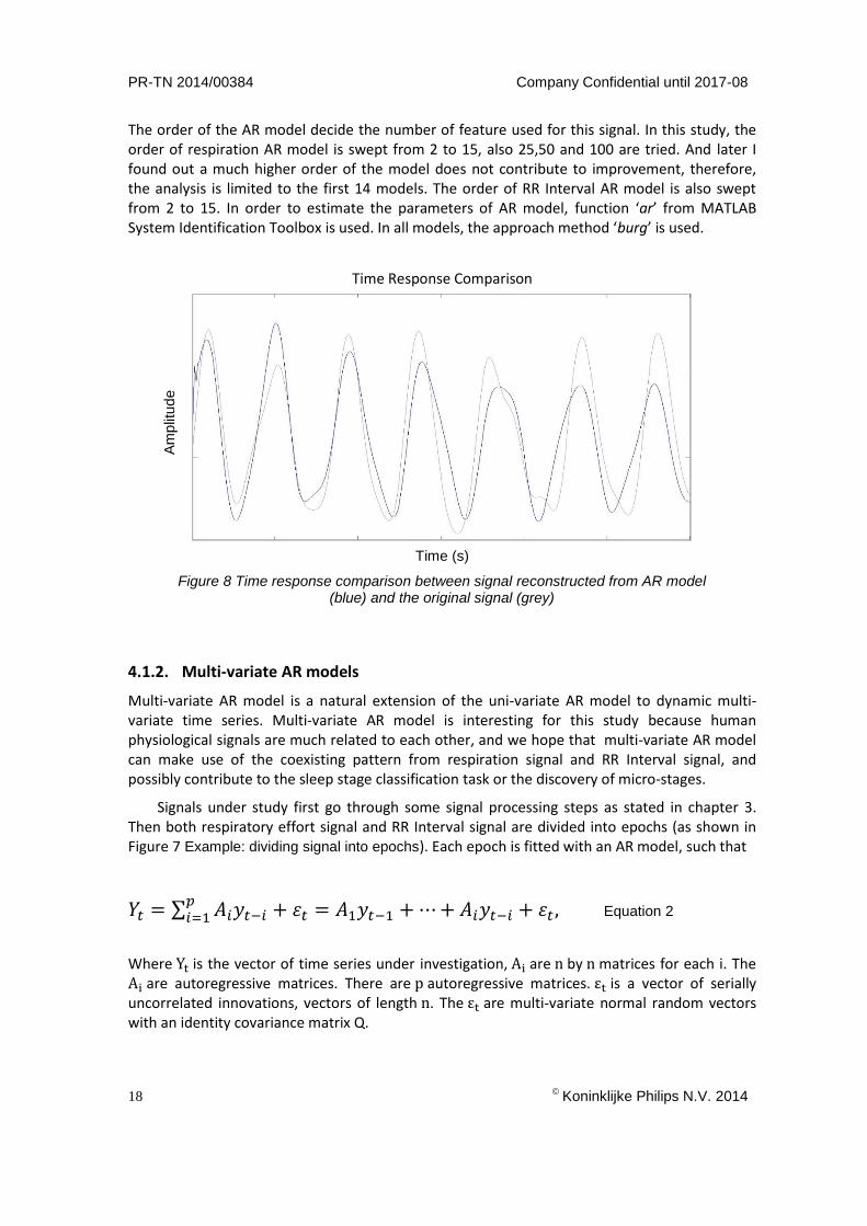
Equation 1), an example on the result of fitting process can be seen in Figure 8.

Figure 7 Example: dividing signal into epochs


18


The order of the AR model decide the number of feature used for this signal. In this study, the order of respiration AR model is swept from 2 to 15, also 25,50 and 100 are tried. And later I found out a much higher order of the model does not contribute to improvement, therefore, the analysis is limited to the first 14 models. The order of RR Interval AR model is also swept from 2 to 15. In order to estimate the parameters of AR model, function ‘ar’ from MATLAB System Identification Toolbox is used. In all models, the approach method ‘burg’ is used.

Time Response Comparison

Time (s)

Figure 8 Time response comparison between signal reconstructed from AR model (blue) and the original signal (grey)

4.1.2. Multi-variate AR models

Multi-variate AR model is a natural extension of the uni-variate AR model to dynamic multi-variate time series. Multi-variate AR model is interesting for this study because human physiological signals are much related to each other, and we hope that multi-variate AR model can make use of the coexisting pattern from respiration signal and RR Interval signal, and possibly contribute to the sleep stage classification task or the discovery of micro-stages.

Signals under study first go through some signal processing steps as stated in chapter 3. Then both respiratory effort signal and RR Interval signal are divided into epochs (as shown in Figure 7 Example: dividing signal into epochs). Each epoch is fitted with an AR model, such that

𝑌𝑡 = ∑ 𝐴𝑖𝑦𝑡−𝑖 + 휀𝑡 = 𝐴1𝑦𝑡−1 + ⋯ + 𝐴𝑖𝑦𝑡−𝑖 + 휀𝑡 ,𝑝𝑖=1 Equation 2

Where Yt is the vector of time series under investigation, Ai are n by n matrices for each i. The Ai are autoregressive matrices. There are p autoregressive matrices. εt is a vector of serially uncorrelated innovations, vectors of length n. The εt are multi-variate normal random vectors with an identity covariance matrix Q.

Am

plit

ud

e



19

Since there are 2 signals, the autoregressive matrices Ai are 2 by 2 square matrices, which can be diagonal or full. In the initial model selection process, the order of multi-variate AR models is swept from 4 to 15, each model has one version as its Ai matrix is full rank and anoth-er version as its Ai matrix is diagonal matrix. To estimate the parameters of multi-variate AR models, function ‘vgxset’ from MATLAB Econometrics Toolbox is used.

The resulting 24 models are selected by several model selection tests. Some preliminary results are as following:

VAR8diag: lowest prediction error VAR9diag: reach lowest AIC value VAR12diag: best model in likelihood ratio test VAR15diag: lowest estimation error Unfortunately, there was not enough time to compute different orders of multi-variate AR models from the complete database. Signal used to select the multi-variate AR models are typical epochs from respiration signal and RR Interval signal.


20


4.2. Gaussian Mixture Model

4.2.1. Model contruction

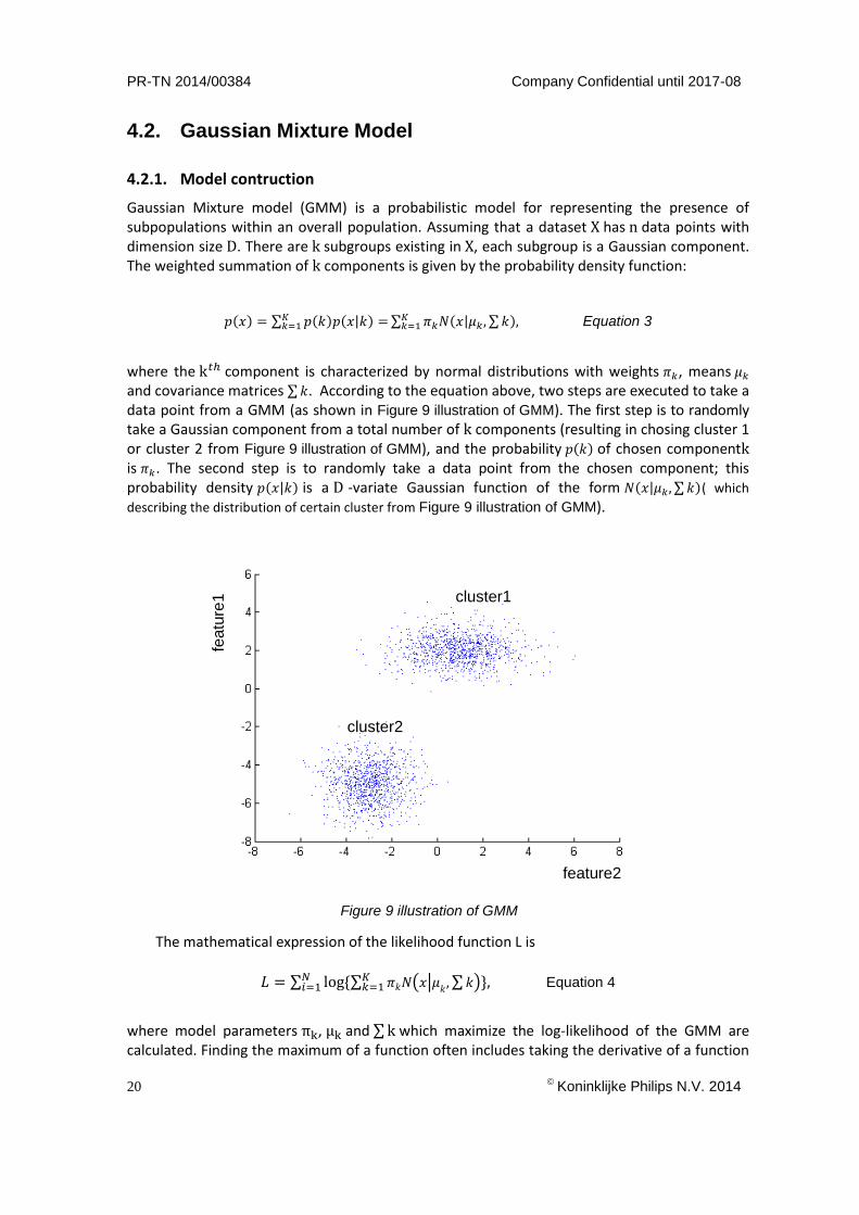
Gaussian Mixture model (GMM) is a probabilistic model for representing the presence of subpopulations within an overall population. Assuming that a dataset X has n data points with dimension size D. There are k subgroups existing in X, each subgroup is a Gaussian component. The weighted summation of k components is given by the probability density function:

𝑝(𝑥) = ∑ 𝑝(𝑘)𝑝(𝑥|𝑘) =𝐾𝑘=1 ∑ 𝜋𝑘𝑁(𝑥|𝜇𝑘, ∑ 𝑘),𝐾

𝑘=1 Equation 3

where the k𝑡ℎ component is characterized by normal distributions with weights 𝜋𝑘, means 𝜇𝑘 and covariance matrices ∑ 𝑘. According to the equation above, two steps are executed to take a data point from a GMM (as shown in Figure 9 illustration of GMM). The first step is to randomly take a Gaussian component from a total number of k components (resulting in chosing cluster 1 or cluster 2 from Figure 9 illustration of GMM), and the probability 𝑝(𝑘) of chosen component k is 𝜋𝑘. The second step is to randomly take a data point from the chosen component; this probability density 𝑝(𝑥|𝑘) is a D -variate Gaussian function of the form 𝑁(𝑥|𝜇𝑘, ∑ 𝑘)( which

describing the distribution of certain cluster from Figure 9 illustration of GMM).

The mathematical expression of the likelihood function L is

𝐿 = ∑ log {∑ 𝜋𝑘𝑁(𝑥|𝜇𝑘, ∑ 𝑘)𝐾

𝑘=1 }𝑁𝑖=1 , Equation 4

where model parameters πk, μk and ∑ k which maximize the log-likelihood of the GMM are calculated. Finding the maximum of a function often includes taking the derivative of a function

cluster1

cluster2

featu

re1

feature2

Figure 9 illustration of GMM



21

and solving for the parameter being maximized. The likelihood function factors into a product of individual likelihood functions, the logarithm of this product is a sum of individual logarithms, and the derivative of a sum of terms is often easier to compute than the derivative of a product. Therefore, it is more convenient to work with the natural logarithm of the likelihood function[29].

4.2.2. Evaluation criteria

To evaluate the quality of Gaussian clusters, several criteria are used. They are Akaike infor-mation criterion (AIC), Purity, Normalized mutual information (NMI) and Rand Index (RI). As an internal criterion, AIC measures the trade-off between the goodness of fit for the model and its complexity. AIC can be computed as

𝐴𝐼𝐶 = 𝑙𝑜𝑔𝑉 + 2𝑝

𝑛, Equation 5

where V is the loss function, p is the number of estimated parameters, and n is the number of values in the estimation dataset. The loss function V is defined by the following equation:

𝑉 = 𝑑𝑒𝑡(1

𝑛∑ 휀(𝑡, 𝜃𝑛)(𝜖(𝑡, 𝜃𝑛))𝑇𝑛

1 , Equation 6

Where θn represent the estimated parameters. A lower AIC value stands for a better model, since in that case, the model has a good trade-off between goodness of fit and model parsimo-ny.

As an external criterion, purity evaluates the agreement between clustering results and PSG-based annotations, the purity can be computed as

𝑃𝑢𝑟𝑖𝑡𝑦(𝛺, 𝐶) = 1

𝑛∑ 𝑚𝑎𝑥|𝜔𝑘 ∩ 𝑐𝑗| ,𝑘 Equation 7

where Ω is the set of clusters, C is the set of labels, ω is the majority group within one cluster, and n is the total number of data point. To compute purity, each cluster is assigned to the label which is most frequent in the cluster, and then the accuracy of this assignment is measured by counting the number of correctly assigned documents and dividing by n. A perfect clustering has a purity of 1. However, a high purity can be easily achieved when the number of clusters is large. The reason is at a high cluster number, every cluster contains a very small amount of data point, for the extreme case, one cluster contains only one data point, in this case, the purity of this cluster is 1.

NMI is another criterion that measures the trade-off between the cluster qualities, against the number of clusters:

𝑁𝑀𝐼(𝛺, 𝐶) = 𝐼(𝛺,𝐶)

𝐻(𝛺)+𝐻(𝐶), Equation 8

I(Ω, C) is mutual information,

𝐼(𝛺, 𝐶) = ∑ ∑ 𝑃(𝑗𝑘 𝜔𝑘 ∩ 𝑐𝑗)𝑙𝑜𝑔𝑃(𝜔𝑘∩𝑐𝑗)

𝑃(𝜔𝑘)𝑃(𝑐𝑗), Equation 9

where𝑃(𝜔𝑘), 𝑃(𝑐𝑗) , and 𝑃(𝜔𝑘 ∩ 𝑐𝑗) are the probabilities of a data point being in cluster 𝜔𝑘, label set 𝑐𝑗, and in the intersection of 𝜔𝑘 and 𝑐𝑗 respectively. Mutual information measures how much

information the presence of a term contributes to make the correct classification decision on label set 𝐶.

)(H and )(CH are the entropies of each set:


22


𝐻(𝛺) = − ∑ 𝑃(𝜔𝑘)𝑙𝑜𝑔𝑃(𝜔𝑘).𝐾 Equation 10

Entropy is a measure of uncertainty, it value increases if the number of clusters increases.

When cluster number 𝑘 equals data number 𝑛, )(H reaches its maximum nlog . ),( CI in

equation 11 does not penalize large cardinalities, the normalization by the denominator

)()( CHH fixes this problem.

Another interpretation of clustering is to see it as a series of decisions. A true positive (TP) decision assigns two similar data points to the same cluster; a true negative (TN) decision assigns two dissimilar data points to different cluster. As a bad decision, a false positive (FP) decision assigns two dissimilar points to the same cluster; a false negative assigns two similar points to different clusters. Criterion for measuring the percentage of correct decisions is the Rand Index:

𝑅𝐼 = 𝑇𝑃+𝑇𝑁

𝑇𝑃+𝐹𝑃+𝐹𝑁+𝑇𝑁, Equation 11

It measures the percentage of decisions that are correct, or the accuracy of the clustering.

4.2.3. GMM evaluation

There are three approaches to perform a GMM clustering on the dataset, they are unsupervised clustering, supervised clustering and semi-supervised clustering. A major difference of these approaches is whether the PSG-based scoring result is used in the clustering dataset. By using evaluation criteria mention in 4.2.2, the cluster number are selected. The selection results are shown in the table below:

GMM AIC NMI RI Purity

Unsupervised 4 6 5 5

Supervised 15 10 10 16

Semi-supervised 7 5 6 10

*numbers in table indicate the number of clusters which gives highest performance

This selection is only looking at the performance of clusters with respect to the R&K sleep stages, which is a interim result, because the final selection on cluster number is also depending on the performance of classifiers.



23

4.3. Feature extraction

4.3.1. Existing features:

A large number of existing features have been extracted previously. In total, 146 features are included in this study, 4 of which are cardiorespiratory coupling features, 101 are cardiac fea-tures and the remaining 41 are respiratory features. Cardiac and respiratory activities are intri-cately lined both functionally as well as anatomically, such characteristics are represented by cardiorespiratory coupling (CRC) features [30]. For example, the spectral coherence between respiration and ECG is one of the CRC features. The cardiac features are extracted based on RR-intervals and the respiratory features include statistical measures derived from both the respir-atory signal waveform and its frequency. These features contain sleep stage information both in the time domain and the frequency domain. More details about the existing features can be found in our previous publications [12], [31]

In order to find a feature set for a specific classification task, which gives the maximum discriminative power with minimal feature redundancy, a correlation-based feature selection method with forward search (CFS-FS) [4] is applied. The algorithm looks for a set of features where each feature is highly correlated with the class, yet uncorrelated with each other.

4.3.2. AR features:

AR features are the features extracted from the AR fitting process. In particular, the signals under study are preprocessed and divided into 30-s epochs, where each epoch is fitted by an AR model and resulting in a polynomial. The AR coefficients from the polynomial are used as AR features to express the characteristics of that particular epoch. In this thesis, the AR models which constructed from respiration effort signal are called RE-ARn1; the AR models which con-structed from RR-interval signal are called RR-ARn2. Where n1, n2 are the orders of the AR models.

Because the number of AR features is determined by the number of coefficients from the fitted polynomial, the selection of AR orders determines the number of AR features. For classifi-cation tasks, criterion one-way analysis of variance Ftest (one-way ANOVA F-test) [32] is used to determine the models order (indicating the number of AR features). It is computed by

𝐹 =∑ 𝑛𝑖(𝑋𝐼 −��)2/(𝐾−1)𝑘

𝑖

∑ (𝑋𝑖𝑗 −𝑋𝐼 )2

/(𝑁−𝐾)𝑛𝑖𝑗

Equation 12

where in the numerator, 𝑛𝑖 represents the number of observations within the ith group, 𝑋𝐼 denotes the sample mean of the ith group, and �� represents the overall mean of the data. The upper part of the equation can be seen as the variability between 𝐾 groups. In the denominator, 𝑋𝑖𝑗 is the jth observation in the ith group, and 𝑁 is the overall sample size. The lower part of the

equation can be understood as the variability within a group. ANOVA F-test can select the AR model which gives the highest discriminate power between multiple classes.

In order to examine AR features’ discriminative power for binary classification, the absolute standardized mean difference (ASMD) is used. It defined as

𝐴𝑆𝑀𝐷 =𝜇1−𝜇2

√𝜎12+𝜎2

2 Equation 13


24


where 𝜇1 and 𝜇2 represent the class mean, 𝜎12 and 𝜎2

2 represent the variances of the classes. When the feature has a large inter-class difference and a small intra-class difference, a high ASMD value is obtained. With these criteria, we could verify the discriminative power of AR features. By comparing the classification performance before and after adding the AR features to the existing features, we can find out if they can help improve classification performance.

4.4. Classification

As mentioned, we consider several classification tasks here. They are multi-class classification of W, R, L, and D (WRLD), and binary classifications including W-detection, R-detection, and D-detection.

In order to estimate how well a classifier performs in practice, a 10-fold cross-validation procedure is used. In the procedure, data is randomly divided into 10 folds where each fold has equal number of subjects/recordings. During each iteration of the 10-fold cross-validation, 9 folds of data are used to train the classifier and the remaining fold is used for testing. Each epoch of the data set contains manually annotated sleep scores, which indicates the true sleep stage of that epoch. The predictions of the classifier on the testing set are compared with the annotations. The results are then averaged over all subjects.

A feature could be good for classifying REM and NREM but bad for multi-class classification. For example, the feature reflecting body movements works well in separating sleep and wake but it might be useless for detection deep sleep. In order to find out the specialty of the AR features, different classification tasks are experimented, as well as different classifiers are used in the process.

4.4.1. Linear Discriminant

We use an LD classifier [33], [34] in the initial attempt of validating the AR features, since fea-tures derived from physiological data seldom follow a normal distribution in a strict manner. An LD classifier is more robust in a way that it is less sensitive to possible violations of basic as-

sumptions of normality. For a given feature 𝑓, the linear discriminant function is given by

𝑔𝑎(𝑓) = −1

2(𝑓 − 𝜇𝑎)𝑇 ∑ (𝑓 − 𝜇𝑎) + 𝑙𝑛 (𝑃(𝜔𝑎))−1 Equation 14

where 𝜇𝑎 is the mean vector for class 𝜔𝑎; ∑ is the covariance matrix, which is assumed to be identical for all classes. The term 𝑃(𝜔𝑎) stands for bias or threshold in the data. In this case, this term is the prior probability of each class.

4.4.2. GMM-HMM classifier

The topic of sleep staging using cardiorespiratory signals is not new and has been studied since the past decade. However, those studies assumed that sleep stages over night are independent so that they did not take information regarding sleep stage transitions into account. A GMM-HMM classifier can exploit the information about sleep stage transitions in time course.

HMM is a statistical model which is especially known for its ability in temporal pattern recognition [35]. It defines a probabilistic structure for reasoning states relations over time, where we wish to recover a series of sleep stages from the epoch-based AR features.



25

Let

𝑇 = length of the observation series,

𝑄 = {𝑞0, 𝑞1, … , 𝑞𝑁−1} = states of the Markov process,

𝑉 = {0, 1, … , 𝑀 − 1} = set of possible observations,

𝐴 = state transition probabilities,

𝐵 = observation probability matrix,

𝜋 = initial state distribution,

𝑂 = (𝑂0, 𝑂1, … , 𝑂𝑇−1) = observation sequence.

A HMM is specified as 𝜆 = (𝐴, 𝐵, 𝜋 ), the transition matrix𝐴 = {𝑎𝑖𝑗}, with 𝑁 × 𝑁elements

where 𝑎𝑖𝑗 = 𝑃 ( 𝑠𝑡𝑎𝑡𝑒 𝑞𝑖 𝑎𝑡 𝑡 + 1 | 𝑠𝑡𝑎𝑡𝑒 𝑞𝑖 𝑎𝑡 𝑡),

The emissions matrix 𝐵 = { 𝑏𝑗(𝑘) }, with 𝑁 × 𝑀 elements where

𝑏𝑗(𝑘) = 𝑃 ( 𝑜𝑏𝑠𝑒𝑟𝑣𝑎𝑡𝑖𝑜𝑛 𝑘 𝑎𝑡 𝑡 | 𝑠𝑡𝑎𝑡𝑒 𝑞𝑗 𝑎𝑡 𝑡).

The HMM classifier finds a state sequence to maximize 𝑃(𝑄|𝑂, 𝜆), given observations 𝑂 = {𝑜1, … , 𝑜𝑡} , and given model 𝜆. Define auxiliary variable 𝛿,

𝛿𝑡(𝑥) = 𝑚𝑎𝑥 𝑃 (𝑞0, 𝑞1, … , 𝑞𝑡 = 𝑥 | 𝑜1, 𝑜2, … , 𝑜𝑡 , 𝜆 ) Equation 15

where δt(x) is the probability of the most probable path ending in state qt = x. Intuitively, the HMM classifier obtain an observation sequence, transition and emission matrix from features of the training set. As a new observation sequence is given by features of the testing set, we calcu-late the probability that the feature from testing set is in a particular state based on the knowledge from training set.

To accurately generate the sequence of observations, GMM is used. It is a probabilistic model for representing the presence of sub-populations within an overall population. GMM has density estimation for each cluster, and is flexible in choosing the component distributions, which allows an arbitrary number of clusters.

Assuming that a feature set 𝑥 has 𝑛 epochs (i.e., data points) with feature number 𝐷 (i.e., dimension size). There are 𝐾subgroups existing in x, each subgroup is a Gaussian component. The weighted summation of 𝐾 components is given by the probability density function

𝑝(𝑥) = ∑ 𝑝(𝑘)𝑝(𝑥|𝑘) = 𝐾𝑘=1 ∑ 𝜋𝑘𝛮(𝑥|𝜇𝑘, ∑𝑘),𝐾

𝑘=1 Equation 16

where the 𝑘𝑡ℎ component is characterized by a normally distributed kernel with weight 𝜋𝑘, mean 𝜇𝑘, and

covariance matrix ∑𝑘. The mathematical expression of the likelihood function 𝐿 is

𝐿 = ∑ 𝑙𝑜𝑔 {∑ 𝜋𝑘𝛮(𝑥|𝐾𝑘=1

𝑁𝑖=1 𝜇𝑘, ∑𝑘)}, Equation 17

where model parameters 𝜋𝑘, 𝜇𝑘, and ∑𝑘 which maximize the log-likelihood of the GMM are calculated. Finding the maximum of a function often includes taking the derivative of a function and solving for the parameter being maximized.

The likelihood function factors into a product of individual likelihood functions, the loga-rithm of this product is a sum of individual logarithms, and the derivative of a sum of terms is


26


often easier to compute than the derivative of a product. Therefore, it is more convenient to work with the natural logarithm of the likelihood function[29].

4.4.3. Evaluation criteria

There are several ways to examine the performance of a classifier. For example, for W-detection, a measure could be the percentage of correctly identified wake epochs (sensitivity) or the percentage of correctly identified sleep epochs (specificity), where wake is considered the positive class. However, the sleep and wake epochs are not equally distributed throughout the night. This imbalanced class distribution could introduce bias in the measure of performance by only judging on the right wrong percentage, and lead to an inappropriate estimation [36]. Therefore, we compute the Cohen’s Kappa coefficient of agreement (κ) as the evaluation criteria [3]. The equation for computing κ is given by

𝜅 = 𝑃𝑟(𝑎)−𝑃𝑟 (𝑒)

1−𝑃𝑟 (𝑒) Equation 18

where Pr(𝑎) is the probability of observed agreement, and Pr (𝑒) is the hypothetical probability of chance agreement. To explain the meaning of κ, a confusion matrix is displayed below:

Classified Result Positive Negative

Annotation Positive TP TN

Negative FP FN

Table 1: Confusion matrix

The classified results and annotations are categorized into positives and negatives with respect to a binary classification. Assuming there are n observations, the probability of observed agreement is:

𝑃𝑟(𝑎) =𝑡𝑝+𝑡𝑛

𝑛; Equation 19

the probability of chance agreement is:

𝑃𝑟(𝑒) = (𝑡𝑝+𝑓𝑝)(𝑡𝑝+𝑓𝑛)+(𝑓𝑝+𝑡𝑛)(𝑓𝑛+𝑡𝑛)

𝑛2 , Equation 20

Cohen’s Kappa criterion takes into account the agreement occurring by chance, and is generally thought to be a more robust measure than simple agreement calculations.



27

5. Exploration of micro-stages

5.1. Clustering

In order to explore the distribution of the clusters and possible micro-stages, the traditional sleep stages are not of main focus anymore. The appropriate AR model order is selected to optimize the describing of the physiological data distribution as closely as possible. Akaike Information Criterion (AIC) is used to select the AR features for clustering purpose. It is comput-ed as

𝐴𝐼𝐶 = 𝑙𝑜𝑔𝑉 + 2𝑝

𝑛, Equation 21

where V is the loss function, p is the number of estimated parameters, and n is the number of observations in the data set. AIC measures the trade-off between the goodness of fit and the complexity.

An AR model is selected to extract RE-AR features (Section IV-A2); one AR model is selected for extract RRAR features. Both extracted RE-AR and RR-AR features are pooled together to represent the combined cardiorespiratory characteristic described by these two modalities. In this report, the combined feature set is called C-AR features. The clustering process is carried out on the selected RE-ARn1, RR-ARn2 and C-ARn3 feature sets separately. The cluster number is selected to have maximum agreement between subjects. The aim is to show that cardi-orespiratory signals can provide more information about micro-sleep stages than the standard-ized R&K stages. This is demonstrated on a task of finding maximum agreement in cluster distri-bution between subjects, and possible mappings with R&K stages.

5.2. Between-subject agreement

The traditional PSG-based sleep stages are obtained by independent visual scoring of sleep experts. For those epochs they did not agree during the scoring process, they usually sit togeth-er and make a consensus. A study on the agreement of data clusters between subjects should allow us to uncover more information from the clusters.

To find out the agreement between all subjects, each subject’s AR features are clustered by a GMM. The main goal is to determine a cluster number which gives the maximum match in distributions between all subjects. Assume that the parameter of cluster number is called k, increasing k without penalty will always reduce the amount of error in each subject’s clustering result, where in the extreme case each data point is considered as one cluster. Therefore, the optimal choice of k requires a balance between clustering accuracy and over-fitting. In this study, the number of clusters is swept from 1 until 30, which resulting in 30 GMMs for each subject. Selecting a k which is larger than 30 may consider to be over-fitting the clustering model, and also complicates the process of interpreting the meaning of the clusters. Two methods are used to measure the match of cluster distributions between subjects. First method uses AIC score of the fitted GMM as evaluation criterion to find the optimal cluster number of all subjects. Second method is to calculate the minimum Mahalanobis distance between cluster pairs from different subjects.


28


5.3. Computation of Between-subject agreement

5.3.1. AIC

Using the GMM’s AIC score is straightforward. For one subject, 30 AIC scores are calculated from 30 GMMs, which resulting in an AIC score curve for this subject. The best cluster number comes from the lowest AIC score (Equation 13). 82 subjects generate 82 different curves; an average over 82 subjects’ results gives the optimal cluster number for all subjects.

5.3.2. Minimum Mahalanobis distance

Mahalanobis distance is a multi-dimensional measure of the distance between two distributions. The distance is zero if two distributions have the same mean, and grows when one moves away from another. For each dimension, the Mahalanobis distance measures the number of standard deviations from two distribution means, at the same time takes into account the correlations of the two sets. Assume an distribution 𝑥 = (𝑥1, 𝑥2, … 𝑥𝑁)𝑇 and distribution 𝑦 = (𝑦1, 𝑦2, … 𝑦𝑁)𝑇 have covariance matrix S, the Mahalanobis distance is defined as

𝐷𝑀(𝑥, 𝑦) = √(𝑥 − 𝑦)𝑇𝑆−1(𝑥 − 𝑦). Equation 22

Assume that x and y are two clusters from two different subjects, a lower DM represents a loser distribution in space, which can be seen as a good match.

Due to the between-subject variability in physiology, the first step of calculating the mini-mum Mahalanobis distance is normalization. The mean of one subject’s clustering data is calcu-lated as following:

𝐶𝑠𝑢𝑗𝑏𝑒𝑐𝑡(𝑖)=

𝜇1 + 𝜇2+ … + 𝜇𝑘𝑘

Equation 23

where 𝜇 is the mean of each cluster, and 𝑘 is the number of clusters. Once the value of 𝐶 is obtained, it is subtracted from all data points from this subject.

After normalization, pairwise comparisons between all 82 subjects are performed, which yields 3321 comparisons (81+80+...+1). For each comparison, two subjects are selected, where a cluster from subject one is considered a match with a cluster from subject two if the distance between their means is the minimum. Assume that subjecta has clusters 𝐶𝑎 = {𝐶𝑎1, 𝐶𝑎2, … , 𝐶𝑎𝑗, … , 𝐶𝑎𝑘}, subjectb has clusters 𝐶𝑏 = {𝐶𝑏1, 𝐶𝑏2, … , 𝐶𝑏𝑗, … , 𝐶𝑏𝑘}. The match

searching process looks for the distance 𝐷, which defined as

𝐷 = min{||𝐶𝑎𝑗 − 𝐶𝑏𝑗

||}

where D is the minimum distance between cluster means, 𝐶𝑎𝑗 and 𝐶𝑏𝑗

are the means of the

clusters. Once a pair of clusters is formed, they are both excluded from the match searching process so that the matching between 𝑘 pairs of clusters is a one to one mapping. The Ma-halanobis distance between two matched clusters is then calculated

(𝐷𝑀(𝑥, 𝑦) = √(𝑥 − 𝑦)𝑇𝑆−1(𝑥 − 𝑦). Equation 22). The result from one comparison is the average Mahalanobis distance of all clusters.



29

As cluster number k becomes bigger, some special cases may occur. In case a cluster has no elements, this cluster and its paired cluster are skipped in the comparison. Another possible case is that the number of elements in a cluster could be smaller than the data dimension (refer to Section 4.2 Gaussian Mixture Model). Since Mahalanobis distance is preserved under full-rank linear transformations of the space spanned by the data, the sample size of a distribution should not be smaller than its own dimension. In such case, all elements in the cluster will be copied the least integer amount of times so that the number of elements in one cluster is larger than the data dimension. Intuitively, this process can be considered as an up-sampling proce-dure.

The minimum Mahalanobis distance for certain cluster number 𝑘 is the average result over 3321 comparisons. It is the average Mahalanobis distance between clusters resulting from choosing cluster number 𝑘. Since the calculation is based on the distance between matched clusters, a smaller distance stands for a good match.

After preliminary visual inspection of the result, as the cluster number grows from 1 to 30, the Mahalanobis distance have shown a growing trend. This observation is reasonable since a larger cluster number produces variations between subjects, which in turn produce cluster mismatches, and resulting in a larger Mahalanobis distance. For a better inspection, we detrended the curves by putting less penalty for higher cluster numbers.


30




31

6. Results and Discussion

6.1. Part I: sleep stage classification results

6.1.1. AR feature normality test results:

For the normality test, 42 AR models are used to extract features from respiration effort signal and from RR-interval signal. Among models which are constructed from the preprocessed respi-ration effort signal, model RE-AR9 produces features which have a skewed distribution; model RE-AR10 produces features which have a binomial distribution. Among models which are con-structed from the first-order derivative of the respiration effort signal, model RE-AR8 produces skewed distribution; model RE-AR9, RE-AR12 and RE-AR15 produce binomial distribution. All 14 RR-AR models produce normally distributed features. For a total of 42 AR models, 86% (36 out of 42) of the models produce normally distributed features, 5% (2 out of 42) of the models produce features with a skewed distribution, and 10% (4 out of 42) of which produce features with a binomial distribution.

For the purpose of sleep stage classification, AR models constructed from the differentiated respiration effort signal have a better performance, therefore results from the models which are constructed from the respiration effort signal without taking the first order derivative are ex-cluded in this thesis.

6.1.2. AR feature selection

The AR feature selection includes: RE-AR selection and RR-AR selection. The discriminative

power of AR models are examined (Section 4.3.2 AR features:).

RE-AR selection The ANOVAF score of RE-AR models are shown in Figure 10 ANOVAF score from different RE-AR models for WLDR classification.. In this figure, the maximum score is obtained from RE-AR4. Model RE-AR9, RE-AR10, RE-AR12 and RE-AR13 also give good ANOVAF scores. We used RE-AR4 since the model uses less parameters, and the features extracted using RE-AR4 provide a better discriminative power than those produced by other AR models.

Figure 10 ANOVAF score from different RE-AR models for WLDR classification.


32


RR-AR selection The ANOVAF score of RR-AR models are shown in Figure 11 ANOVAF score from different RR-AR

models for WLDR classification.. The high scores occur at model RR-AR5 and RR-AR8, and level off at the other models. Comparing RR-AR5 and RR-AR8, we select RR-AR5, because it uses less parameters, and the features extracted by this model provide higher discriminative power.

Figure 11 ANOVAF score from different RR-AR models for WLDR classification.

6.1.3. AR feature evaluation

To evaluate AR features, we compute the discriminative power of 9 AR features (4 features extracted by model RE-AR4, 5 features extracted by model RR-AR5) and all 147 existing features; then inspect resulting rankings. Since there are many features, we only briefly discuss the rank-ing result in this thesis.

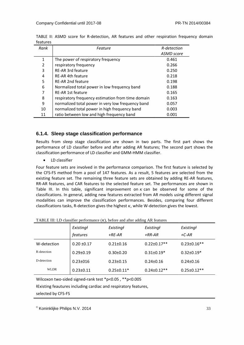
Firstly, all features’ ANOVAF scores for WLDR classification are calculated. AR features have a highest ranking of 86 among all features. Then the ranking of discriminative power for W-detection, R-detection, and D-detection are examined. For W-detection, AR features have a highest ranking of 37; for R-detection, AR features’ highest ranking is at 62, and for D-detection, AR features’ highest ranking is 76. In general, AR features do not have high discriminative power comparing with all existing features. However, since each AR model is linked to the frequency distribution of the data, it is reasonable that we compare AR features with other frequency domain features. As a result, we found that RE-AR features have higher discriminative power for R-detection comparing with other respiration frequency domain features. Table II listed the ASMD score of R-detection for features used in the comparison. There are 11 features involved, 4 of which are extracted by RE-AR4. It can be observed that among respiration frequency do-main features, RE-AR features give a good performance in distinguishing REM and other sleep stages.



33

TABLE II: ASMD score for R-detection, AR features and other respiration frequency domain features

Rank Feature R-detection ASMD score

1 The power of respiratory frequency 0.461 2 respiratory frequency 0.266 3 RE-AR 3rd feature 0.250 4 RE-AR 4th feature 0.218 5 RE-AR 2nd feature 0.198 6 Normalized total power in low frequency band 0.188 7 RE-AR 1st feature 0.165 8 respiratory frequency estimation from time domain 0.163 9 normalized total power in very low frequency band 0.057

10 normalized total power in high frequency band 0.003 11 ratio between low and high frequency band 0.001

6.1.4. Sleep stage classification performance

Results from sleep stage classification are shown in two parts. The first part shows the performance of LD classifier before and after adding AR features; The second part shows the classification performance of LD classifier and GMM-HMM classifier.

LD classifier

Four feature sets are involved in the performance comparison. The first feature is selected by the CFS-FS method from a pool of 147 features. As a result, 5 features are selected from the existing feature set. The remaining three feature sets are obtained by adding RE-AR features, RR-AR features, and CAR features to the selected feature set. The performances are shown in Table III. In this table, significant improvement on 𝜅 can be observed for some of the classifications. In general, adding new features extracted from AR models using different signal modalities can improve the classification performances. Besides, comparing four different classifications tasks, R-detection gives the highest 𝜅, while W-detection gives the lowest.

TABLE III: LD classifier performance (𝜅), before and after adding AR features

Existingƚ

features

Existingƚ

+RE-AR

Existingƚ

+RR-AR

Existingƚ

+C-AR

W-detection 0.20 ±0.17 0.21±0.16 0.22±0.17** 0.23±0.16**

R-detection 0.29±0.19 0.30±0.20 0.31±0.19* 0.32±0.19*

D-detection 0.23±016 0.23±0.15 0.24±0.16 0.24±0.16

WLDR 0.23±0.11 0.25±0.11* 0.24±0.12** 0.25±0.12**

Wilcoxon two-sided signed-rank test *p<0.05 , **p<0.005

ƚExisting feautures including cardiac and respiratory features,

selected by CFS-FS


34


Comparison of LD and GMM-HMM

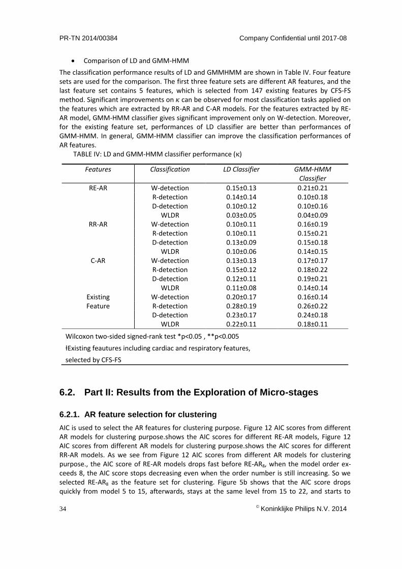
The classification performance results of LD and GMMHMM are shown in Table IV. Four feature sets are used for the comparison. The first three feature sets are different AR features, and the last feature set contains 5 features, which is selected from 147 existing features by CFS-FS method. Significant improvements on 𝜅 can be observed for most classification tasks applied on the features which are extracted by RR-AR and C-AR models. For the features extracted by RE-AR model, GMM-HMM classifier gives significant improvement only on W-detection. Moreover, for the existing feature set, performances of LD classifier are better than performances of GMM-HMM. In general, GMM-HMM classifier can improve the classification performances of AR features.

TABLE IV: LD and GMM-HMM classifier performance (κ)

6.2. Part II: Results from the Exploration of Micro-stages

6.2.1. AR feature selection for clustering

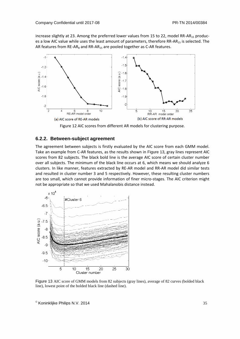
AIC is used to select the AR features for clustering purpose. Figure 12 AIC scores from different AR models for clustering purpose.shows the AIC scores for different RE-AR models, Figure 12 AIC scores from different AR models for clustering purpose.shows the AIC scores for different RR-AR models. As we see from Figure 12 AIC scores from different AR models for clustering purpose., the AIC score of RE-AR models drops fast before RE-AR8, when the model order ex-ceeds 8, the AIC score stops decreasing even when the order number is still increasing. So we selected RE-AR8 as the feature set for clustering. Figure 5b shows that the AIC score drops quickly from model 5 to 15, afterwards, stays at the same level from 15 to 22, and starts to

Features Classification LD Classifier GMM-HMM Classifier

RE-AR W-detection 0.15±0.13 0.21±0.21 R-detection 0.14±0.14 0.10±0.18 D-detection 0.10±0.12 0.10±0.16

WLDR 0.03±0.05 0.04±0.09 RR-AR W-detection 0.10±0.11 0.16±0.19

R-detection 0.10±0.11 0.15±0.21 D-detection 0.13±0.09 0.15±0.18

WLDR 0.10±0.06 0.14±0.15 C-AR W-detection 0.13±0.13 0.17±0.17

R-detection 0.15±0.12 0.18±0.22 D-detection 0.12±0.11 0.19±0.21

WLDR 0.11±0.08 0.14±0.14 Existing Feature

W-detection 0.20±0.17 0.16±0.14 R-detection 0.28±0.19 0.26±0.22 D-detection 0.23±0.17 0.24±0.18

WLDR 0.22±0.11 0.18±0.11

Wilcoxon two-sided signed-rank test *p<0.05 , **p<0.005

ƚExisting feautures including cardiac and respiratory features,

selected by CFS-FS



35

increase slightly at 23. Among the preferred lower values from 15 to 22, model RR-AR15 produc-es a low AIC value while uses the least amount of parameters, therefore RR-AR15 is selected. The AR features from RE-AR8 and RR-AR15 are pooled together as C-AR features.

Figure 12 AIC scores from different AR models for clustering purpose.

6.2.2. Between-subject agreement

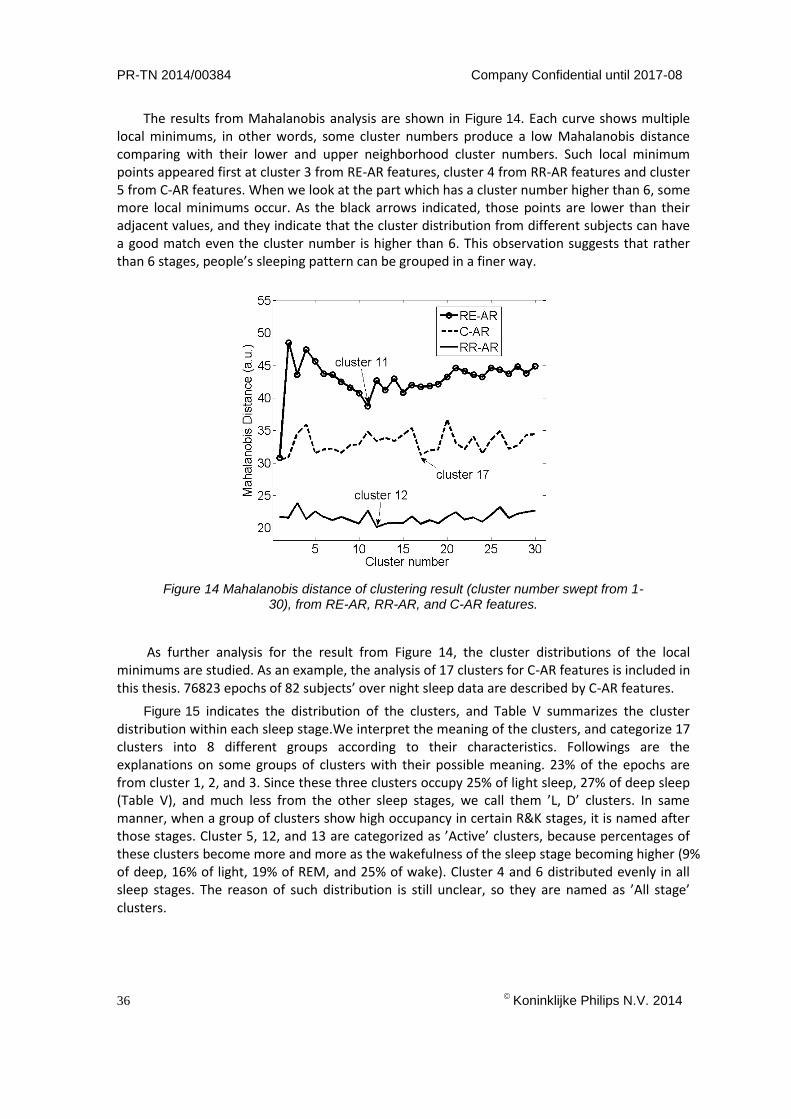
The agreement between subjects is firstly evaluated by the AIC score from each GMM model. Take an example from C-AR features, as the results shown in Figure 13, gray lines represent AIC scores from 82 subjects. The black bold line is the average AIC score of certain cluster number over all subjects. The minimum of the black line occurs at 6, which means we should analyze 6 clusters. In like manner, features extracted by RE-AR model and RR-AR model did similar tests and resulted in cluster number 3 and 5 respectively. However, these resulting cluster numbers are too small, which cannot provide information of finer micro-stages. The AIC criterion might not be appropriate so that we used Mahalanobis distance instead.

Figure 13 AIC score of GMM models from 82 subjects (gray lines), average of 82 curves (bolded black

line), lowest point of the bolded black line (dashed line).


36


The results from Mahalanobis analysis are shown in Figure 14. Each curve shows multiple local minimums, in other words, some cluster numbers produce a low Mahalanobis distance comparing with their lower and upper neighborhood cluster numbers. Such local minimum points appeared first at cluster 3 from RE-AR features, cluster 4 from RR-AR features and cluster 5 from C-AR features. When we look at the part which has a cluster number higher than 6, some more local minimums occur. As the black arrows indicated, those points are lower than their adjacent values, and they indicate that the cluster distribution from different subjects can have a good match even the cluster number is higher than 6. This observation suggests that rather than 6 stages, people’s sleeping pattern can be grouped in a finer way.

Figure 14 Mahalanobis distance of clustering result (cluster number swept from 1-30), from RE-AR, RR-AR, and C-AR features.

As further analysis for the result from Figure 14, the cluster distributions of the local minimums are studied. As an example, the analysis of 17 clusters for C-AR features is included in this thesis. 76823 epochs of 82 subjects’ over night sleep data are described by C-AR features.

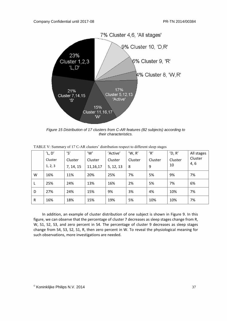
Figure 15 indicates the distribution of the clusters, and Table V summarizes the cluster distribution within each sleep stage.We interpret the meaning of the clusters, and categorize 17 clusters into 8 different groups according to their characteristics. Followings are the explanations on some groups of clusters with their possible meaning. 23% of the epochs are from cluster 1, 2, and 3. Since these three clusters occupy 25% of light sleep, 27% of deep sleep (Table V), and much less from the other sleep stages, we call them ’L, D’ clusters. In same manner, when a group of clusters show high occupancy in certain R&K stages, it is named after those stages. Cluster 5, 12, and 13 are categorized as ’Active’ clusters, because percentages of these clusters become more and more as the wakefulness of the sleep stage becoming higher (9% of deep, 16% of light, 19% of REM, and 25% of wake). Cluster 4 and 6 distributed evenly in all sleep stages. The reason of such distribution is still unclear, so they are named as ’All stage’ clusters.



37

Figure 15 Distribution of 17 clusters from C-AR features (82 subjects) according to their characteristics.

TABLE V: Summary of 17 C-AR clusters’ distribution respect to different sleep stages

’L, D’

Cluster

1, 2, 3

’S’

Cluster

7, 14, 15

’W’

Cluster

11,16,17

’Active’

Cluster

5, 12, 13

’W, R’

Cluster

8

’R’

Cluster

9

’D, R’

Cluster 10

All stages Cluster 4, 6

W 16% 11% 20% 25% 7% 5% 9% 7%

L 25% 24% 13% 16% 2% 5% 7% 6%

D 27% 24% 15% 9% 3% 4% 10% 7%

R 16% 18% 15% 19% 5% 10% 10% 7%

In addition, an example of cluster distribution of one subject is shown in Figure 9. In this figure, we can observe that the percentage of cluster 7 decreases as sleep stages change from R, W, S1, S2, S3, and zero percent in S4. The percentage of cluster 9 decreases as sleep stages change from S4, S3, S2, S1, R, then zero percent in W. To reveal the physiological meaning for such observations, more investigations are needed.


38


7. Conclusions

An exploration of sleep stages based on cardiorespiratory signals is presented in this thesis. We use AR models to extract physiological information from respiratory effort and ECG signals. The AR features show discriminative power among existing cardiorespiratory features, and give improvement in classification performances. Comparing LD and GMM-HMM classifiers, the performance of GMM-HMM is generally higher than the performance of LD when AR features are used. From this observation we speculate that AR features contain the information of sleep stage transitions.

Apart from sleep staging, much emphasis has been put on proving that the R&K rules do not fully describe the sleep stages. The preliminary results from the exploration of micro-stages show that the clusters can be seen as microstages of the sleep structure, the meaning of some clusters can be explained, but for some clusters, their meanings are still unclear. This suggests that more investigations need to be done on exploring the physiological meaning of each cluster.

8. Recommendations

The performance of GMM-HMM is generally higher than the performance of LD when AR fea-tures are used, from which we speculate that AR features containing the information of sleep stage transitions. More exploration can be done on the comparison between GMM-HMM classifier and other classifiers which looking at the time varying property of features, especially on AR features. This kind of study may give us a better understanding on which time scale the AR feature can provide time information of sleep.

To investigate the physiological meaning of each cluster, correlation analysis can be carried out between different physiological signals and the corresponding cluster behavior.



39

A Appendices

Feature involved in this study

14 resp_power_freq_periodogram

15 resp_vlf_periodogram

16 resp_lf_periodogram

17 resp_hf_periodogram

18 resp_lf_hf_periodogram

19 resp_v_5_epochs

20 resp_v_7_epochs

21 resp_v_9_epochs

22 resp_mean_breath_by_breath_corr

23 resp_std_breath_by_breath_corr

24 resp_std_breath_length

25 resp_freq_td

26 ecg_hr_mean

27 ecg_rr_mean

28 ecg_sdnn

29 ecg_rr_range

30 ecg_pnn50

31 ecg_rmssd

32 ecg_sdsd

33 ecg_vlf_norm

34 ecg_lf_norm

35 ecg_hf_norm

36 ecg_lf_hf_ratio

37 ecg_sampen1_scale1




















57 ecg_alpha_1

58 ecg_alpha_2

59 ecg_alpha

60 ecg_alpha_al

61 ecg_pdfa

62 ecg_mean_resp_freq

63 ecg_power_mean_resp_freq

64 ecg_phase_hf_pole

65 ecg_module_hf_pole

66 ecg_rr_mean_detr

67 ecg_wdfa

88 resp_sampen

89 x_resp_ecg_copower

90 resp_activity

91 resp_dtw_dist

94 ecg_power

95 ecg_4th_power

96 ecg_curve_length

97 ecg_nonlin_energy

100 ecg_hjorth_mobility

101 ecg_hjorth_complexity

103 ecg_psd_peak_power

104 ecg_psd_peak_frequ

105 ecg_psd_mean

106 ecg_psd_median

107 ecg_psd_entropy

109 ecg_hurst_exponent

116 x_cwt_activity

119 ecg_rr_percentile10


121 ecg_rr_median



124 ecg_rr_MAD

125 ecg_rr_percentile10_detr



40


127 ecg_rr_median_detr



130 ecg_rr_MAD_detr

131 ecg_hr_percentile10


133 ecg_hr_median



136 ecg_hr_MAD

137 ecg_hr_percentile10_detr


139 ecg_hr_median_detr



142 ecg_hr_MAD_detr

159 x_resp_ecg_phase_coordination_long

160 x_resp_ecg_phase_coordination_short

161 ecg_phase_coordination_long

162 ecg_phase_coordination_short

163 resp_dfw_dist

164 resp_amp_peak_ApEn

165 resp_amp_trough_ApEn

166 resp_amp_peak_sd_mean

167 resp_amp_trough_sd_mean

168 resp_amp_peak_sd_median

169 resp_amp_trough_sd_median

170 resp_amp_pt_dist_median

171 resp_amp_pt_dtw_dist

172 resp_breath_vol_median

173 resp_breath_in_vol_median

174 resp_breath_ex_vol_median

175 resp_breath_fr_median

176 resp_breath_in_fr_median

177 resp_breath_ex_fr_median

178 resp_breath_in_ex_fr_ratio

179 resp_breath_in_ex_time_ratio

180 ecg_hrv_likelihoodratios_mean

181 ecg_hrv_likelihoodratios_median

182 ecg_hrv_likelihoodratios_min

183 ecg_hrv_likelihoodratios_max

200 resp_template_dist_min

201 resp_template_dist_top_mean

202 resp_template_dist_top_std

203 resp_template_dist_mean

204 resp_template_dist_std

205 ecg_teager_energy

206 ecg_teager_size

207 ecg_teager_int_std

208 ecg_teager_int_mean

209 ecg_teager_len_mean_emd

210 ecg_teager_len_std_emd

211 ecg_der_int_std_emd

212 ecg_der_len_std_emd

213 ecg_rr_sign

214 x_resp_ecg_phase_synchronization

215 resp_ar_1_coef

216 resp_ar_2_coef

217 resp_ar_3_coef

218 resp_ar_4_coef

219 ecg_rr_ar_1_coef










41

References

[1] A. Rechtschaffen and A. Kales, “A Manual of Standardized Terminology, Techniques and Scoring System for Sleep Stages of Human Subjects,” 1968.

[2] C. Iber, S. Ancoli-Israel, A. L. Chesson, and S. . Quan, “The AASM Manual for the Scoring of Sleep and Associated Events: Rules, Terminology and Technical Specifications.,” Am. Acad. Sleep Med., 2007.

[3] J. Cohen, “A Coefficient of Agreement for Nominal Scales.,” Educ. Psychol. Meas., no. 20(1), pp. 37–46, 1960.

[4] M. A. Hall, “Correlation-based Feature Selection for Machine Learning,” The University of Waikato, 1999.

[5] S. J. Redmond, P. de Chazal, C. O’Brien, S. Ryan, W. T. McNicholas, and C. Heneghan, “Sleep staging using cardiorespiratory signals,” Somnologie - Schlafforsch. und Schlafmedizin, vol. 11, no. 4, pp. 245–256, Oct. 2007.

[6] N. J. Douglas, D. P. White, C. K. Pickett, J. V Weil, and C. W. Zwillich, “Respiration during sleep in normal man,” Thorax, no. 37(11), pp. 840–844, 1982.

[7] V. K. Somers, D. Phil, M. E. Dyken, A. L. Mark, and F. M. Abboud, “sympathetic-nerve activity during sleep in normal subjects,” N. Engl. J. Med., no. 328(5), pp. 303–307, 1993.

[8] D. J. Pitson and J. R. Stradling, “Autonomic markers of arousal during sleep in patients undergoing investigation for obstructive sleep apnoea, their relationship to EEG arousals, respiratory events and subjective sleepiness.,” J. Sleep Res., vol. 7, no. 1, pp. 53–9, Mar. 1998.

[9] S. Devot, R. Dratwa, and E. Naujokat, “Sleep/wake detection based on cardiorespiratory signals and actigraphy,” IEEE Eng. Med. Biol. Soc., pp. 5089–5092, 2010.

[10] T. Willemen, D. Van Deun, V. Verhaert, M. Vandekerckhove, V. Exadaktylos, J. Verbraecken, S. Van Huffel, B. Haex, and J. Vander Sloten, “An evaluation of cardiorespiratory and movement features with respect to sleep-stage classification.,” IEEE J. Biomed. Heal. informatics, vol. 18, no. 2, pp. 661–669, Mar. 2014.

[11] T. Kirjavainen, D. Cooper, O. Polo, and C. E. Sullivan, “Respiratory and body movements as indicators of sleep stage and wakefulness in infants and young children.,” J. Sleep Res., vol. 5, no. 3, pp. 186–194, Sep. 1996.

[12] X. Long, P. Fonseca, J. Foussier, R. Haakma, and R. M. Aarts, “Using Dynamic Time Warping for Sleep and Wake Discrimination,” Biomed. Heal. Informatics, vol. 25, pp. 886–889, 2012.

[13] A. Bar, G. Pillar, I. Dvir, J. Sheffy, R. P. Schnall, and P. Lavie, “Evaluation of a portable device based on peripheral arterial tone for unattended home sleep studies.,” Chest, vol. 123, no. 3, pp. 695–703, Mar. 2003.

[14] Y.-M. Kuo, T. Dept. of Electr. Eng., Nat. Cheng Kung Univ., Tainan, and J.-S. L. ; P.-C. Chung, “A Visual Context-Awareness-Based Sleeping-Respiration Measurement System,” vol. 14, no. 2, pp. 255–265, 2010.


42


[15] D. Pevernagie, R. M. Aarts, and M. De Meyer, “The acoustics of snoring.,” Sleep Med. Rev., vol. 14, no. 2, pp. 131–44, Apr. 2010.

[16] M. A. Cohn, A. S. Rao, M. Broudy, S. Birch, H. Watson, N. Atkins, B. Davis, F. D. Stott, and M. A. Sackner, “The respiratory inductive plethysmograph: a new non-invasive monitor of respiration,” Bull. Eur. Physiopathol. Respir., no. 18(4), pp. 643–658, 1982.

[17] H. Schulz, “Rethinking Sleep Analysis comment on the AASM manual for the scoring of sleep and associated events,” J. Clin. Sleep Med., vol. 9, no. 4(2), pp. 99–103, 2014.

[18] S. Himanen and J. Hasan, “Limitations of Rechtschaffen and Kales,” Sleep Med. Rev., vol. 4, no. 2, pp. 149–167, 2000.

[19] S. J. Roberts, M. Krkic, I. Rezek, J. Pardey, L. Tarassenko, J. Stradling, and C. Jordan, “The use of neural networks in EEG analysis,” in Proceedings of IEE Colloquium on Sleep Analysis, 1995.

[20] A. Lewandowski, R. Rosipal, and G. Dorffner, “Extracting more information from EEG recordings for a better description of sleep.,” Comput. Methods Programs Biomed., vol. 108, no. 3, pp. 961–972, Dec. 2012.

[21] G. Klosch, B. Kemp, T. Penzel, A. Schlogl, P. Rappelsberger, E. Trenker, G. Gruber, J. Zeitlhofer, B. Saletu, W. M. Herrmann, S. l. Himanen, D. KUNZ, M. J. Barbanoj, J. Roschke, A. Varri, and G. Dorffner, “The SIESTA project polygraphic and clinical database,” IEEE Eng. Med. Biol. Mag., no. 20(3), pp. 51–57, 2001.

[22] D. J. Buysse, C. F. Reynold III, T. H. Monk, S. R. Berman, and D. J. Kupfer, “The Pittsburgh Sleep Quality Index: a new instrument for psychiatric practice and research,” Psychiatry Res., no. 28(2), pp. 193–213, 1989.

[23] J. A. van Alste, W. van Eck, and O. E. Herrmann, “ECG Baseline Wander Reduction Using Linear Phase Filters,” Comput. Biomed. Res., pp. 417–427, 1985.

[24] P. S. Hamilton and W. J. Tompkins, “Quantitative Investigation of QRS Detection Rules Using the MIT/BIH Arrhythmia Database,” Biomed. Eng. (NY)., vol. BME-33, no. 12, pp. 1157–1165, 1986.

[25] P. Fonseca, J. Foussier, R. M. Aarts, and X. Long, “A novel low complexity post-processing algorithm for precise QRS localization,” 2014.

[26] G. Box, G. M. Jenkins, G. C. Gwilym, and G. C. Reinsel, Time Series Analysis: Forecasting and Control (3rd ed.). 1994.

[27] H. Akaike, “Power spectrum estimation through autoregressive model fitting,” Ann. Institue Stat. Math., vol. 21, pp. 407–419, 1969.

[28] C. M. Bishop, “Mixtures of Gaussians,” in Pattern Recognition and Machine Learning, 2006, pp. 430–432.

[29] A. W. F. Edwards, Likelihood. Cambidge: Cambridge University Press, 1992.

[30] A. J. Garcia III, J. E. Koschnitzky, T. Dashevskiy, and J.-M. Ramirez, “Cardiorespiratory coupling in health and disease.,” Auton. Neurosci., vol. 175, no. 1–2, pp. 26–37, Apr. 2013.



43

[31] X. Long, J. Foussier, P. Fonseca, R. Haakma, and R. M. Aarts, “Respiration amplitude analysis for REM and NREM sleep classification.,” Conf. Proc. ... Annu. Int. Conf. IEEE Eng. Med. Biol. Soc. IEEE Eng. Med. Biol. Soc. Annu. Conf., vol. 2013, pp. 5017–20, Jan. 2013.

[32] A. Ross, “Soft Biometrics for Surveillance : An Overview,” 2013.

[33] J. P. Marques de sa, Pattern Recognition, Concepts, Methods and Applications. 2011, pp. 90–108.

[34] J. H. Friedman, “Regularized Discriminant,” J. Am. Stat. Assoc., no. 84(405), pp. 165–175, 1988.

[35] B. Obermaier, C. Guger, C. Neuper, and G. Pfurtscheller, “Hidden Markov models for online classiification of single trial EEG data,” Pattern Recognit. Lett., vol. 22, pp. 1299–1399, 2001.

[36] H. He and E. A. Garcia, “Learning from Imbalanced Data,” IEEE Trans. Knowl. Data Eng., vol. 21, no. 9, pp. 1263–1284, Sep. 2009.

Technical Note PR-TN 2014/00384 · The receiver of such a report must ensure ... Technical Note:...

Documents

Transcript of Technical Note PR-TN 2014/00384 · The receiver of such a report must ensure ... Technical Note:...