cOco

!

ZI--

ii

NASA TN D-886

TECHNICALD-886

NOTE

THEORY OF AN ELECTROMAGNETIC MASS ACCELERATOR

FOR ACHIEVING HYPERVELOCITIES

By Karlheinz Thom and Joseph Norwood, Jr.

Langley Research Center

Langley Field, Va.

NATIONAL AERONAUTICS AND SPACE ADMINISTRATION

WASHINGTON June 1961

https://ntrs.nasa.gov/search.jsp?R=19980227779 2020-01-28T08:46:38+00:00Z

IS

NATIONAL AERONAUTICS AND SPACE ADMINISTRATION

TECHNICAL NOTE D-886

THEORY OF AN ELECTROMAGNETIC MASS ACCELERATOR

FOR ACHIEVING HYPERVELOCITIES

By Karlheinz Thom and Joseph Norwood, Jr.

SUMMARY

It is shown that for any electromagnetic accelerator which employs

an electromagnetic force for driving the projectile and uses the pro-

jectile as the heat sink for the energy dissipated in it by ohmic heating,

the maximum velocity attainable without melting is a function of the mass

of the projectile. Therefore, for hypervelocities a large projectile

mass is required and thus a power supply of very large capacity is nec-

essary. It is shown that the only means for reducing the power require-

ment is maximizing the gradient of the mutual inductance. In the scheme

of the sliding-coil accelerator investigated herein, the gradient of the

mutual inductance is continuously maintained at a high value. It is also

shown that for minimum length of the accelerator, the current must be

kept constant despite the rise in induced voltage during acceleration.

The use of a capacitor bank as an energy source with the condition that

the current be kept constant is investigated.

Experiments at low velocities are described.

INTRODUCTION

The experimental investigation of impacts at hypervelocities (from

about 15 km/sec to 72 km/sec) is currently of much interest. Various

schemes for achieving such velocities in the laboratory have been inves-

tigated. Systems where the electromagnetic force is employed for an

acceleration are reviewed, for instance, in reference i. In such elec-

tromagnetic systems the projectile is basically a conductor in a mag-

netic field, and it is propelled by the interaction of the current which

flows through it and a magnetic field which is generated by another part

of the electrical circuit. The ohmic heating of the projectile thus

appears as the main problem of electromagnetic acceleration, and it is

because of this heating effect that hypervelocities have not yet been

achieved through electromagnetic acceleration. The theoretical treat-

ments of the previous electromagnetic accelerators_ however, did not

proceed to a general relation between the effect of ohmic heating and

2

the maximumvelocity which can be achieved. Deriving such a generalrelation is the main purpose of this paper. From this relation the limi-tations of electromagnetic acceleration should be derivable, and the mainfeatures of a feasible schemeshould be deducible.

SYMBOLS

a

A

b

B

c

C

d

E

F

H

I

L

m

M

N

n

P

R

t

coil diameter, m

area, m 2

distance of separation of coil ends, m

magnetic flux density, webers/m 2

distance of separation of coil cel.ters, m

capacitance, farads

diameter of wire, m

electric field strength, volts/m

force, newtons

heat, Joules

current, amp

length, m

self-inductance, henries

mass, kg

mutual inductance, henries

number of turns

number of turns per unit length, i/m

power, watts

ohmic resistance, ohms

time, sec

L

i

i

59

L

i

i

59

T

v

V

W

x, y, z

7

_t

T

Subscripts :

a

e

i

k

m

0

max

i

2

i, 2, 3 •

temperature, OK

velocity (also x), m/sec

voltage_ volts

energy, joules

coordinate of system, with x as distance in direction

of acceleration, m

constants (defined in eqs. (I0))

specific heat, joules/kg OK

difference

permeability, henries/m

electrical conductivity, mhos/m

tensile strength, newtons/m 2

integral multiple of separation time of coils, sec

magnetic flux, webers

accelerator

end

induced

mechanical

magnetic

applied, initial

maximum

refers to coil i, the driving coil

refers to coil 2, the driven coil

number of steps in divided capacitor bank

A bar over a symbol indicates meanor average value.symbol indicates differentiation with respect to time t.symbol indicates differentiation with respect to distance

A dot over aA prime on aX.

GENERAL RELATIONS

The general relation between the ohmic leating of the projectile

and the maximum velocity which can be achiew:_d by electromagnetic accel-

eration is derived in the present section. }_sically, in all schemes of

electromagnetic acceleration the projectile is a conductor in a magnetic

field, and it is propelled by the electromagnetic force. The current

flowing through the projectile heats it. Th_Ls, acceleration is possible

only as long as the projectile does not melt

Assume that the process of acceleration is short in time, so that

no cooling mechanism can become effective, he projectile then is the

heat sink. The case where the projectile is extremely small is excluded.

The rate of ohmic heating of the projectile Ls then given by the

equation

Rl2dt = 7m dT (1)

where R stands for the ohmic resistance, It is the increment of time,

7 is the specific heat, m is the mass of zhe projectile, and dT is

the rise in temperature.

The driving force derives from the gradLent of the magnetic field

energy. If the driving circuit and the circuit represented by the pro-

jectile are connected in series and if the f_rce acts in the x-direction,

the force is given by the equation

F = ½ (2)

where the total inductance of the system is L = LI + L2 f 234 and con-

sists of the self-inductance LI of the driving circuit, the self-

inductance L2 of the projectile, and twice their mutual inductance M.

The velocity of the projectile is obtained by integrating the force

equation (eq. (2)):

$0 tF= _ dt

= 1 12 dL dt (5)2 dx m

L

i

i

59

L

i

i

59

From equation (I) the time variable can be replaced by the change of

temperature. Inserting this parameter into equation (3) yields

Ti dL7 dT

=_ TO_(4)

The velocity now appears as a function of the temperature, and the maxi-

mum velocity attainable is readily obtained by extending the integral to

the melting temperature of the projectile.

Z

With R = _, where

cross-section area, and

Z is the length of the conductor, A

is the conductivity, the velocity is

is the

! _/_melt _ A

2 $ TO dx Z

o7 dT

dLA

dx

maximum velocity

The greatest velocity obviously is obtained, when the expression

continuously remains at its highest possible value. Then, for

%ax 1 (_ _) _ Tmelt= -- oy dT

2 max TO

(5)

The integral on the right-hand side depends only on the properties of

the material of which the projectile consists. The integral, therefore,

has to be considered as a material constant. Since the expression in

front of the integral determines the geometrical configuration of the

accelerator, including its size, it is seen from equation (5) that there

is no similarity in electromagnetic acceleration.

If the magnitude of the parenthesized expression is to be found as

a function of the velocity desired, equation (5) can be divided by the

material constant A(aTT) to obtain

2_

In the electromagnetic cgs system of units, inductance has the

dimension of length, expressed in centimeters. The right-hand side of

equation (6) thus represents a characteristic length, and this length

appears as a linear function of the velocity desired.

For a certain velocity the expression \8< must be constant. Itmaybe concluded, therefore, that the charact_ristic length expressed byequation (6), can be considered as the cube root of a volume that the

projectile must have in order to achieve a certain desired velocity. For

copper and for _max = 2 × 10 6 cm/sec, (dL_ 7) _ 0.2cm.A (For this eval-

uation, the dependency of a and 7 on the _emperature has not been

considered. A rigorous computation will result in a somewhat larger

value for the characteristic length.) The minimum weight of the pro-

jectile is then of the order of grams. In the hypervelocity range the

kinetic energy that must be delivered to the _>rojectile is in the mega-

joule range. Such a large quantity of energy should be transferred in

a very short time, if the accelerator is to h_ve a tolerable length. An

electromagnetic hypervelocity mass accelerator', therefore, fundamentally

requires an enormous power input.

The derivation of a characteristic length for the electromagnetic

acceleration (eq. (6)) represents, of course, an order-of-magnitude

evaluation. A closer study of the expression (_ _I reveals that a

fundamental improvement for electromagnetic a_celeration can be achieved

dL

only through maximizing the _ factor with regard to its dependency

on x. Increases in the inductance gradient by increasing the length,

for instance, would basically be cancelled by the increase of the

length Z in the denominator of the right-hand side in equation (6).

An efficient electromagnetic accelerator, therefore, requires a scheme

which provides a continuous high value of the dL parameter; that is,dx

one in which the driving and the driven condu_tors continuously stay

close together.

From integration of the force equation (:_), it is seen immediately

that the shortest distance over which the coil is accelerated can be

obtained when the current continuously remains at its highest possible

value. There is an upper limit for the current, because the magnetic

stresses have to be balanced by the strength ,_f the material.

From the requirements for maximum velocity for the smallest pro-

Jectile possible and for the shortest length of the accelerator, it may

be concluded that an electromagnetic accelerator should keep the con-

ductors of the driving and driven circuits col_tinuously close together

and furnish a continuous maximum current. Or_ from a more practical

point of view, a good electromagnetic accelerator should feature a con-

stant maximum value of the gradient of the mu_ual inductance, and a

L

i

i

5

9

voltage matching should be provided in order to maintain the current

at its highest permissible magnitude.

THEORY OF THE SLIDING COIL ACCELERATOR

L

i

i

5

9

In the attempt to design an apparatus which comes close to these

requirements, a scheme is suggested which can be called a "sliding-coil

accelerator." (See fig. i.) Basically, the sliding-coil accelerator

employs two coils, which attract or repel each other. One coil, coil i,

is the stationary one, the long driving coil. The driven coil is identi-

fied as coil 2; it is short and slightly larger in cross section than

the driving coil so that it is free to move across the stationary coil.

The driven coil 2 picks up the current from a parallel rail by

means of a sliding contact. Via another sliding contact, coil 2 feeds

the current at its end into the driving coil. The driving coil then

completes the circuit. By this arrangement, the driving coil is ener-

gized continuously up to the position of the driven coil. Both coils

magnetically stay close together; thus a high and nearly constant gra-

dient of the inductance is provided.

If the two coils are carefully examined to see how the sliding con-

tact moves from one turn of the driving coil to the next one, it is noted

that the gradient of the inductance is not constant. It varies, instead,

with the small distance by which the two coils are separated, until a

new turn of the driving coil is energized and restores the original

condition.

From computations of the inductance of the system it is found that,

under the condition of small variations of the distance, the average

value of the gradient of the inductance can be defined with sufficient

accuracy by the arithmetic mean:

1 += _ _ b=bma x b=

where b is the distance separating the ends of the two coils.

The maximum distance of separation is here assumed to be the thick-

ness of the wire of which the driving coil is wound. It should be real-

ized, however, that the arcing at the sliding contact may create an

effective distance greater than that. The average gradient of the induc-

tance then decreases, and the performance of the system, consequently,

8

will decrease also. The problem of arcing may not be too serious, how-

ever, because the interaction of the longitudinal current in the arc

with the radial component of the magnetic field will produce a magnetic

blowout effect.

The maximum current for the sliding-coil accelerator has to be

derived from the requirement that the magnetic forces will not rupture

the coils. A formula, which relates the ten_ile Strength of the wire

to the magnetic stresses has been developed by Miller, Dow, and Haddad

(ref. 2) and is shown in a subsequent summary of the equations for the

sliding-coil accelerator.

The current can be kept constant by controlling the applied voltage.

As the projectile becomes accelerated, it generates an electromotive

force. The induced voltage and the conditior; for constant current can

be derived from the power equation

_WmV0I = I2R + BY + F_I (7)

where VO is the applied voltage, Wm is the magnetic-energy storage,

and i is the velocity. On the average (see appendix A) the magnetic

energy storage of the system is assumed to be constant. Then 8Wm/St

is zero. With the force equation (2), the power equation (7) yields

R 1 dLi)vo :I +_ (8)

which is the condition to be used for keeping the current constant.

Multiplying the parenthetical expression by the current I gives as

the second term the induced voltage, averaged over several cycles of

coil separation and subsequent switching.

L

i

i

9

POWER SOURCES

If equation (6) is used for achieving a velocity of some 20 km/sec,

a minimum mass of the projectile of the order of several grams is seen

to be required. To accelerate this mass up t_ meteorite velocities over

a length suitable for laboratory work require3 a power input of the order

of millions of kilowatts. Obviously, an energy storage device is more

economical than a generator for such high power. A capacitor bank for

energy storage seems to be advantageous and i_s use as power source is

investigated.

9

L

i

i

5

9

For keeping the current constant, as required by equation (8), the

voltage must increase along the path of acceleration. On the other hand_

a capacitor bank will decrease its voltage while expending energy.

In order to match the requirements of equation (8) with the charac-

teristic of a capacitor bank_ two schemes of arrangement are suggested.

The first scheme may be called the "divided capacitor bank." It con-

sists of a number of capacitors hooked up in series. At each subsequent

junction of two capacitors, an increasing potential against ground is

established. The second scheme makes use of one big capacitor. The

increasing voltage according to equation (8) is matched by an arrange-ment of resistors.

The Divided Capacitor Bank

The scheme of the divided capacitor bank is represented in figure 2.

The path of acceleration is divided into a large number of small steps

of length dx. The length dx shall be larger than the distance between

adjacent turns on the driving coil_ it is small as compared with the

length of the accelerator. The amount of energy transferred to the

system while the projectile travels the distance dx will correspond-

ingly be a small fraction of the total energy expenditure. The treat-

ment of the energy relations by using calculus_ therefore, can be

expected to be a sufficiently good approximation.

The increment of energy added to the system while the projectile

travels the distance dx is obtained from the power equation as

12fR )dw:(9)

where

_laL2dx

This energy must be furnished by discharging the capacitors; thus,

(io)

dW = CV dV (il)

The combination of equations (9) and (ii) yields the voltage drop

across the capacitor bank due to the energy expenditure for moving the

propelled coil the distance dx at a total distance x from the origin:

lO

dV:c--_ (12)

The voltage which the capacitor bank furnishes at a distance x

from the origin then is the difference between the initial voltage to

which it was charged at the position x and tile voltage drop due to

the acceleration of the projectile up to the p)sition x,

_0 xv(x) = v0(x)- dV (13)

On the other hand, equation (8) must be f/ifilled

V(x) = I(R + 6_)

Since equation (8) requires an increase of the voltage with increasing x,

Vo(x) must be a function of x such that the difference Vo(x) - dV

results in the required V(x) according to equation (8).

Differentiating equation (13) and substituting from equation (8)

gives

v' , i (14)= VO C_

Differentiating equation (8) and substituting in the left side of equa-

tion (14) yields the capacitance as a function of the length:

c(x)= I_+,_

Vo-_--

(15)

The function VO in the denominator of equation (15) is still

arbitrary. Evidently the charging voltage V0 depends on the size of

the capacitors. The smaller the capacitance, the higher is V0 in

order to satisfy equation (14). A steep function V_ consequently,

according to equation (15), results in a steeper decrease of the added

capacitance with the length. From consideratfon of the increase of the

induced voltage with increasing velocity, the limitation of the increase

of V0 becomes apparent.

L

i

i

59

ll

L

1

1

9

!

If V0 is assumed to increase with _, the capacitance C

decreases approximately with 1/x. For larger values of x the curve C

has a very small slope. In this case, the decrease of the total capaci-

tance will be very slight as the distance increases:

i _ I + i (16)CZ+ I CZ

and because of the small slope

CZ+ I _ C z

It follows, then, that C _ _.

(16a)

When CZ+ I is the total capacitance at step Z+I, then CZ is

the total capacitance at step Z and C is the individual capacitance

which is added when the propelled coil passes the (Z+l)th step.

From equations (16) and (16a), it can be seen that the capacitances

CZ have to become increasingly large. The scheme of the divided capac-

itor bank appears feasible. Whether it is economical will depend on

particular requirements.

The Capacitor Bank With a Resistor in Line

The capacitor bank with a resistor in line (fig. 3) avoids the dis-

advantage of the divided capacitor bank, the requirement of greatly

increasing capacitances.

In this arrangement, the voltage V 0 is the voltage across the

single unit capacitor bank and is also a function of the position of

coil 2. In contrast to the scheme described for the divided capacitor

bank, the capacitance is constant. Instead, the resistance is a func-

tion of the length. If the employed resistance is considered much

larger than the resistance of the coils, apart from the conditions at

the very end of the accelerator, the resistance of the coils may be

neglected. If the condition for constant current (eq. (8)) is utilized,

it is seen that the function V 0 coincides with V as used before:

v : I(R + _) (17)

The power input into the system by discharging the capacitor bank,

by accelerating the projectile, and by generating heat in the resistoris

-CV dV = RI + F_dt

R

12

(__-CV dxd-_V= 12 R + _i

Differentiating equation (17) gives

(18)

dV - I(---_+ R') (19)_x 2_

The combination of equations (18) and (19) delivers a differential equa-

tion for the resistance R as a function of the length

and by integration

The integration constant R0

where V0

tot R

or

R = R 0 - _ +

is the resistance of

_ VOR0 -_-

is the initial charging voltage.

is zero.

(21)

R at x = 0

At the end of the accelera-

Then, when Z denotes the length of the accelerator

I

21 _ +- (23)Vo = _ C,,

Equation (23) delivers the charging voltage of the capacitor bank.

Since the magnitudes m, _, _, and I are fixed by the demand for

obtaining a desired velocity, the charging v(itage V0 depends on the

capacitance. At the limit as C _ _, equation (23) yields

2I _ _ (24)vo = -_ -/

13

L

1

1

59

and the initial resistance R0

bank is

for the case of a very large capacitor

Ro= (25)

Apparently the initial resistance of the system must equal the final

impedance. Thus, 50 percent or more of the energy stored in the capaci-

tor bank is lost when the scheme described here is used.

According to equation (25), there is a freedom of choice between

the size of the capacitor bank and the amount of the initial voltage to

which the bank must be charged. The choice will depend on the require-

ments of practical cases and will basically represent a compromise

between high voltage problems and problems of efficiency.

Equation (8) requires that the voltage at the end of the accelera-

tion be

ve = (261

Dividing equation (23) by equation (26) and solving for C yields

an equation for the capacitance depending on the ratio of the initial

voltage V 0 and the voltage after the acceleration is completed:

c = 2 1 (27)

If, for instance, V 0 is chosen to be twice Ve, the capacitance

has to be 2/c_. A greater ratio Vo/V e apparently does not improve

V 0the system; with m = 2j the bank will be discharged by 75 percent.

V e

SUMMARY OF FORMULAS AND SAMPLE CALCULATION

Provided friction forces can be neglected, and provided the arcing

at the sliding contacts has no serious effects, the sliding-coil accel-

erator now can be designed.

For the sliding-coil accelerator, the previous relation of maximum

velocity and permissible heating (eq. (5)) becomes:

14

= (o7 2 (28)

The term within the first parentheses on the right-h_d side contains

the gradient of the mutual inductance, the di_eter of the coils, and

the number of turns on the projected coil, N 2. This expression must

be maximized simultaneously. The term within the second parentheses is

maximized by selecting the best material. _Aation (28) thus req_res

a certain _re di_eter d for achieving a particular velocity. (Note

that this procedure requires the assumption t_at a >> d, because then

the dependency of L on d is essentially eii_nated. In the case

_ere the di_eter of the coils a and the wire di_eter d are com-

i d 2parable, _-_2 has to be maximized. This case is, however, not

considered favorable for the sliding-coil accelerator because the

_/_ par_eter wo_d decrease appreciably.)

The maximum current under the condition that the magnetic stresses

will not rupture the coils may be obtained from a formula derived by

Dow, Miller, and Haddad in reference 2:

n1°t > °ge T + += _d 2

(29)

where n is the number of turns per unit length.

With the magnitude of the current known, the length _ of the

accelerator can be determined from the following equation:

_ m

z TdaL (3o)dx

Using a capacitor bank as power supply snd a variable resistor for

the voltage matching, the capacitance must be determined from equation (27)

Vo

where the final voltage Ve is determined by equation (26). The resis-

tance as a function of the length is given by equation (21). The charging

L

i

i

5

9

15

L

1

1

59

voltage V0 can be determined from compromising between high-voltage

problems and the desire to keep the capacitor bank small.

With copper selected as the wire material, a sample calculation for

achieving a velocity of 20 km/sec, has been carried out. The character-

istic values are

Current, amp ........................ 1.76 × 104

Diameter of coils, m .................... 2.5 x 10 -2

Thickness of wire, m .................... 2 × 10 -3

Weight of projectile, kg .................. 3 × i0-5

Length of accelerator, m .................. 40

Capacitor bank, f ..................... 4 × 10 -3

Charging voltage, v .................... 5.5 × 104

From these values it can be seen that the construction of a full-

size accelerator would require considerable technical effort.

EXPERIMENTAL WORK

As the energy relations indicate, a full-size accelerator would

require an enormous energy storage device. In addition, the accelera-

tor should consist of a large track built in a highly precise manner.

For extremely high velocities the track must be constructed inside a

vacuum tank. Because of the technical problems involved, constructionof a full-size accelerator was not undertaken. Instead a small-scale

model of the sliding-coil accelerator has been built for verifying the

principles derived.

The Apparatus

For energy storage, a capacitor bank was used. Its capacitance was

2,500 microfarads and it was capable of storing 5,000 Joules at a voltage

of 2,000 volts.

The driving coil of the accelerator was built by winding an

AWG 23 enameled copper wire on a bakelite rod of 3/4-inch (1.9 cm)

diameter. The length of this coil was l0 inches (25 cm).

The driven coils were wound of the same wire. Samples incorpo-

rating 5, i0, and 15 turns have been fired. The driven coils had a

diameter slightly greater than that of the driving coil, so as to allow

them to slide freely along the driving coil.

16

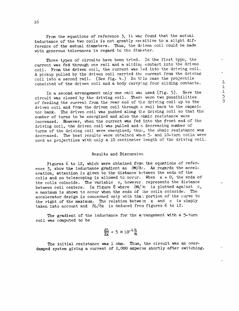
From theequations of reference 3, it was found that the mutual

inductance of the two coils is not greatly ser sitive to a slight dif-

ference of the mutual diameters. Thus, the dliven coil could be made

with generous tolerances in regard to the diszeter.

Three types of circuits have been tried. In the first type, the

current was fed through one rail and a slidin_ contact into the driven

coil. From the driven coil, the current was ]ed into the driving coil.

A pickup pulled by the driven coil carried th_ current from the driving

coil into a second rail. (See fig. 4.) In t_is case the projectile

consisted of the driven coil and a body carrying four sliding contacts.

In a second arrangement only one rail was used (fig. 5)- Here the

circuit was closed by the driving coil. There were two possibilities

of feeding the current from the rear end of the driving coil up to the

driven coil and from the driven coil through s, rail back to the capaci-

tor bank. The driven coil was pushed along the driving coil so that the

number of turns to be energized and also the ohmic resistance were

increased. However, when the current was fed into the front end of the

driving coil, the driven coil was pulled and _ decreasing number of

turns of the driving coil were energized; thu_, the ohmic resistance was

decreased. The best results were obtained wh_n 5- and lO-turn coils were

used as projectiles with only a i0 centimeter length of the driving coil.

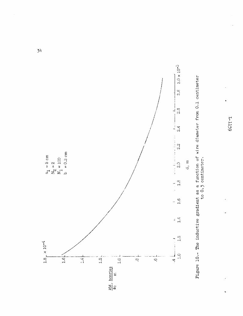
Results and Discussion

Figures 6 to 12, which were obtained fr_l the equations of refer-

ence 5, show the inductance gradient as _M/_. As regards the accel-

eration, attention is given to the distance b_tween the ends of the

coils and no telescoping is allowed to occur. When x = O, the ends of

the coils coincide. The variable c, however represents the distance

between coil centers. In figure 8 where _M/i)c is plotted against c,

a maximum is shown to occur when the ends of ]he coils coincide. The

accelerator design is concerned only with tha_ portion of the curve to

the right of the maximum. The relation between x and c is simply

taken into account and _L/Sx is deduced fr_a figures 6 to 12.

The gradient of the inductance for the a?rangement with a 5-turn

coil was computed to be

_L = 5 X i0-_dx m

The initial resistance was i ohm. Thus, the circuit was an over-

damped system giving a current of 2,000 amperes shortly after switching.

_S

17

F_L

L

The linear dependency of the resistance in the experimental setup

does not deviate too much from the second-order dependency as required

by the theory outlined before, so long as the distances involved are not

too large. The actual variation of the current is estimated in the order

of not greater than 1:2.

The approximation of a constant force in the experimental setup may

furthermore be Justified by the fact that the gradient of the mutual

inductance eventually decreases as the coil approaches the end of the

path of acceleration. This effect will, to a certain degree, cancelthe effect of the increase of current. With a constant current of

2,000 amperes and a weight of the projectile of 1 gram

F = !dL 12 = _ × 10-4 × 4 x lO 6 = lO 3 newtons2 dx 2

2F x = 2 × l06 × lO -1 = 20 × lO 4m

and

_ x = 450m

=

Thus, velocities up to 450 meters per second were to be expected.

For a large number of shots made with the test accelerator, the

velocities have been measured simultaneously by a photocell arrangement

and by a ballistic pendulum. Both measurements have been in good coin-

cidence, the pendulum always indicating velocities about l0 percent

smaller than those measured by the photocells. There was, however, a

great spread in the values obtained. Most of the shots gave velocities

in the range of 200 to 300 meters per second. For a number of shots,

velocities were between 300 and 400 meters per second. The velocity

for one shot was measured at 420 meters per second.

This variation in velocity must be attributed to the rather pro-

visional experimental setup. Experience has shown that careful con-

sideration must be given design and construction details, particularly

with regard to the sliding contacts. As a matter of fact, it was

observed that in the cases of failures the projectile was hindered

somewhere along its path of acceleration. As a result, it came out

"off-schedule," and in consequence, both the driven coil and the

driving coll were overloaded and were destroyed.

Another irregularity results from the arcing at the sliding con-

tacts. It is believed that occasionally so much of the wires vaporized

18

that short circuits occurred as a result of a breakdown through the arc.

In such cases almost no energy was transferred into mechanical work of

acceleration. It should be mentioned that the provisional setup did not

afford any features to prevent the vaporization of the copper wire at

the sliding contacts.

According to the theory, an induced volt,age must develop across the

accelerated coil as

Vi _ 12 dxdL_ = 10 3 × 5 × 10 -4 × _ = _ volts

This voltage had to be expected as a residual voltage across the capaci-

tor bank after the shot.

After most of the shots no charge was l_ft in the capacitor bank,

but after a number of firings a voltage was ]eft. The voltage left in

these cases was found to be in a good agreement with the values derived

by the theory, in all cases slightly lower (]0 percent) than the com-

puted values. The failure of the system to yroduce this voltage reading

must again be attributed to a breakdown due to plasma generation at the

sliding contacts.

After having made numerous shots, an observer could, by watching

the brightness of the arcs at the sliding contacts, predict the success

of a shot in advance of the reading of the velocity measurements.

More information of the above-mentioned breakdown phenomena and on

the forces involved in the acceleration could certainly have been obtained

by a direct-current measurement. For safety _easons, such a direct-

current measurement could not have been made _ithout applying consider-

ably more effort than had been planned.

L

i

i

59

CONCLUDING REMARKS

It has been shown that for any electromagnetic accelerator which

employs electromagnetic forces for driving the projectile and where the

projectile is the heat sink for the energy dissipated in it by ohmic

heating, the maximum velocity obtainable without melting is a function

of the mass of the projectile. Therefore, for hypervelocities a larger

projectile mass is required. It has been shown that the only means for

reducing the power requirements is maximizing the gradient of the mutual

inductance. In the scheme of the slidlng-coil accelerator the _radient

of the mutual inductance is continuosly maintained at a high value.

Theoretical treatment has shown that the principles of the sliding-coil

accelerator can be used to achieve hyperveloc_ties through comparatively

19

L

1

1

99

moderate technical efforts. A problem which has not been solved is the

effect of arcing at the sliding contacts at hypervelocities. More infor-

mation on these effects is needed before construction of a full-scale

slidlng-coil accelerator can be attempted. A comprehensive design for

the construction of a hypervelocity electromagnetic mass accelerator

has not been anticipated in the scope of this paper; instead, the basic

relations of scaling are revealed and a suggestion has been developed

which projects the problem of electromagnetic acceleration to hyper-

velocities into the realm of realistic technical possibilities.

Langley Research Center,

National Aeronautics and Space Administration,

Langley Field, Va., March 24, 1961.

2O

APPENDIXA

DERIVATIONOFTHEINDUCEDVOLTAGE

The induced voltage for a conducting boc[ymo_ing with the velocity vwith respect to a magnetic field is derived from

--%

cu_l_ = - __B+ curl(_× _) (m)_t

when the curl of the vector product is expanded and v is assumed con-

stant for a short but finite period of time T, then, with div B = O,equation (AI) becomes

curl E - _t v grad • B (A2)

If the velocity has an x-component only, the x-component of the vector

gradient has to be taken; thus,

Vx(grad • B) x = vx grad Bx

The induced voltage across either one of the two coils of the sliding-

coil accelerator is obtained by applying Stokes' theorem in equation (A2):

vi :- f/ dy _z - _ \ZI-Jx dy dz (A3)

The integration has to be taken over the cro:;s-sectional area of the

coil in a plane perpendicular to x, the dir,_ction of propagation. Thus,

_t Vx 7x (A4)

L

1

1

59

Two cases must now be distinguished. _Le first case describes the

type of accelerator, where four sliding contracts are employed. In this

accelerator, the length of the driving coil (toes not change. (See pre-

vious section "Experimental work," first type of accelerator.) The

second case is applicable to the sliding-coll accelerator with two

sliding contacts, where the length of the driving coll changes with the

position of the driven coil.

21

L1199

In the first case, the length of the driving coil does not change

with the position of the driven coil. With constant current, no net

change takes place in the amount of magnetic flux of the system. The

amount of magnetic energy storage, on the average, is constant.

The induced voltage of the system is the sum of the voltage induced

in coil 2 (the driven coil) and that in coil i (the driving coil). In

a system moving with the velocity v of the propelled coil the switching

mechanism serves to reestablish the magnetic flux after it has changed

because of the separation of the coils. The change of flux through the

driven coil thus is periodic. On the average, over complete cycles of

coil separation and subsequent switchings, there is no net change of

flux through coil 2. The driven coil, therefore, does not show a net

induced voltage.

The induced voltage across the driving coil is

(Vi)l - _t v -_-

where the subscript i refers to coil i. Since in this system the

amount of flux does not change, on the average, due to the switching

mechanism, - 0. There is, however, a displacement of flux with8t

respect to the driving coil; the expression v --8_i is different from8x

zero.

The flux through coil i is

_i = I(LI -+ MI2) (A6)

where LI is the self-inductance of coil i and MI2

inductance. In a system where LI is constant,

_¢____i= ± _MI_____21

_x _x

is the mutual

where the plus or minus sign applies for alike or opposite sense of

winding, respectively. If T is an integral multiple of the time of

1 cycle of coil separation and subsequent switching, the average induced

voltage in coil 1 is

f0 f0-- 1 v I(t) -+ dtvi :¥ vi dt :,¥ -_x

22

With

_MI2- Constant

and

T

y:l I dtT

_MI'_ i dLV--i = vI ---=- =- vI -- (AT)

_x 2 dx

which is also the induced wDltage over the whole system, in accordance

with equation (8).

In the case of the two--sliding-contact systems, the length of the

driving coil (coil i) depends upon the position of the propelled coil,

coil 2. Apart from the conditions at the end or the beginning of the

accelerator (depending on the cases where the principles of repelling

or attracting coils are used), coil ]. can be considered as a long sole-

noid. Then the mutual inductance does not change with the length ofcoil i.

From the definition of the mutual inductance

V'L_

M21 = -r-I].

it follows that

"V2 = -n 2 ff B dy dz

and for the coils close together

i n2r2_l _ n2 (NI) dll2 dt

where 2r = a is the diameter of the coils and ZI is the length of

coil 1. The mutual inductance then is

(AS)

L

i

i

5

9

23

L

1

1

59

An elongation of coil i does not change the ratio NI/Z I. Conse-

quently, a variation of the length of this coil does not change the

mutual inductance. (This result is unaffected by the approximation in

equation (A8).) Therefore, by the same reasoning as given for the pre-

vious system, there is no net change of flux through the driven coil 2,

and on the average there is no induced voltage across coil 2 in the case

of a two-sliding-contact system.

The induced voltage across the driving coil is composed of

v -- (A9)Vi - _t _x

_-:i _LI I because the mutual inductance does not varythe parameter_t _t

with time, and _i _ I ___MMbecause the change of the self-inductance is_x _x

not caused by the separation of the coils but by a subsequent switching

in time.

The second term on the right-hand side of equation (A9) is there-

fore of the same magnitude as in equation (A7) for the four-sliding-

contact system. In the two-sliding-contact system an additional term

I _Ll/_t appears for computing the induced voltage. Equation (8) of

the main text has to be corrected correspondingly.

24

REFERENCES

i. Mannix, W. C., Atkins, W. W., and Clark, R. E., eds.: Proceedings of

the Second Hyperveloeity and Impact Effects Symposium, vol. i,

Dec. 1957. (Sponsored by Naval Res. Lab. and Air Res. Dev.

Command.)

2. Miller, D. B., Dow, W. G., and Haddad, G. E.: An Electromagnetic

Accelerator Utilizing Sequential Switching. Rep. 2522-I0-F

(AFCRC TR 58-267), Res. Inst., Univ. of _chigan, Sept. 1958.

3. Snow, Chester: Formulas for Computing Cap_Lcitance and Inductance.

NBS Circular 544, U.S. Dept. Commerce, 1954.

25

O_

/#

//

/

!

i_

V Sliding contact

_ -\ \

,I f DrivencoilZ

lliliIIli]]]liiTii,'"

JJ i ;i:// Slid nta

Driving coil i

energizedDriving coil I

not energized

Powersupply

Figure i.- Schematic diagram of sliding coil accelerator.

26

V1- i

IVl-2

C l

CI- Ik.nkid

IV3

V1

C3

C2

CI

Figure 2.- The divided capacitor bank.

27

C__A

R(x)

x=O

C

Figure 3.- Capacitor bank with a resistor in line.

28

\o

.,-4

00

(D

A

\\

\\

'\

\\

o

_D

oo

I

(D

!

t_O.rt

%

_n_D

29

Ok_h

C

Figure 5.- Single-rail accelerator.

34

!0

×

L00

E

0

II II II II

//

//

/!

/

/

8

X

0

c_

oo

cO

i

i0

co

T-I

cO

i

]__...... ___2 ........ .J 0

_d

+_(1)

.H

I1)O

,-t

c;

(1)

.H

-H

(D+_

0.H

_)

O

_ 4._

.H

_3%b_

(1)

._-oO

°H

I

o,--t

oH

%n

_D

35

0m

,--ir--I

I0','--'I

X

I..

,---I

0

o __ _ 0 /

II II II rl /

.I ............... I ............. I ................. I ........... L ..........

@

IOr--t

- X

O

_o

o0

o

co

c'a

0 co

4.-}@

°H4,_

{.}

od

{5Eoh

o

©

.r-I

%

o4(1)

o o

4-_ .Hc) 4o

a3'.D

_8a3

o

%

.r4

I

,-t,--t

.r4

36

0__MM,ac

henries

m

i000

800_

600i

400 -

200 -

lOO 80i-

4O

2O

i0

8

6

4

2

_ xlO -6

N 2 = 2

d I = 0.09: cm

d2 = 0.09: cm

N 1 = I00

b =0.2 cm

1 I I I J

0 5 i0 15 20 x 10-2

al, m

Figure 12.- The inductive gradient as a function of diameter of drivingcoil.

._ -L,_ F,,,_,V,. L- 1199