
TECHNICAL NOTE GOCE Level 1B Gravity Gradient Processing ... · from a GRACE gravity eld model...
63
ESA UNCLASSIFIED - Releasable to the Public TECHNICAL NOTE GOCE Level 1B Gravity Gradient Processing Algorithms Prepared by Christian Siemes RHEA for ESA - European Space Agency Reference ESA-EOPSM-GOCE-TN-3397 Issue/Revision 1.0 Date of Issue 27/08/2018 Status Approved
Transcript of TECHNICAL NOTE GOCE Level 1B Gravity Gradient Processing ... · from a GRACE gravity eld model...

ESA UNCLASSIFIED - Releasable to the Public
TECHNICAL NOTE
GOCE Level 1B Gravity Gradient Processing Algorithms
Prepared by Christian Siemes
RHEA for ESA - European Space Agency
Reference ESA-EOPSM-GOCE-TN-3397
Issue/Revision 1.0
Date of Issue 27/08/2018
Status Approved

ESA UNCLASSIFIED - Releasable to the Public
APPROVALTitle GOCE Level 1B Gravity Gradient Processing Algorithms
Issue Number 1.0 Revision Number 0
Author Christian Siemes Date 27/08/2018
Approved by Date of Approval
Rune Floberghagen (EOP-GM)
GOCE and Swarm Mission Man-ager
Bjorn Frommknecht (EOP-GEP)
Payload Data GS Manager
Roger Haagmans (EOP-SME)
GOCE Mission Scientist
CHANGE LOGReason for change Issue Nr. Revision Number Date
Document created 1.0 0 27/08/2018
CHANGE RECORDIssue Number 1.0 Revision Number 0
Reason for change Date Pages Paragraph(s)
Page 2/63
GOCE Level 1B Gravity Gradient Processing Algorithms
Issue Date 27/08/2018 Ref ESA-EOPSM-GOCE-TN-3397
ESA UNCLASSIFIED - Releasable to the Public
Contents
1 Introduction 71.1 Purpose of this document . . . . . . . . . . . . . . . . . . . . . . . . . . . . . . 71.2 How to derive gravity gradients from accelerations . . . . . . . . . . . . . . . . . 71.3 Level 1b processing scheme . . . . . . . . . . . . . . . . . . . . . . . . . . . . . . 8
2 Basic processing elements 132.1 Precision of epochs and time differences . . . . . . . . . . . . . . . . . . . . . . . 132.2 Interpolation . . . . . . . . . . . . . . . . . . . . . . . . . . . . . . . . . . . . . 142.3 Numerical integration . . . . . . . . . . . . . . . . . . . . . . . . . . . . . . . . . 142.4 Numerical differentiation . . . . . . . . . . . . . . . . . . . . . . . . . . . . . . . 15
3 Convention for rotation matrices, quaternions, and angular rates 17
4 Star tracker data processing 214.1 Star tracker data preprocessing . . . . . . . . . . . . . . . . . . . . . . . . . . . 214.2 Star tracker data combination . . . . . . . . . . . . . . . . . . . . . . . . . . . . 21
5 Adjusting the misalignment between star trackers and gradiometer 31
6 Accelerometer data processing 336.1 Accelerometer data calibration . . . . . . . . . . . . . . . . . . . . . . . . . . . . 336.2 Gross outlier detection and removal . . . . . . . . . . . . . . . . . . . . . . . . . 37
7 Angular rate and acceleration reconstruction 437.1 Calculation of star tracker angular rates . . . . . . . . . . . . . . . . . . . . . . 437.2 Calculation of gradiometer angular rates . . . . . . . . . . . . . . . . . . . . . . 447.3 Calculation of filters for angular rate reconstruction . . . . . . . . . . . . . . . . 447.4 Application of filters for angular rate reconstruction . . . . . . . . . . . . . . . . 46
8 Attitude reconstruction 518.1 Mathematical derivation of algorithm . . . . . . . . . . . . . . . . . . . . . . . . 518.2 Covariance matrix . . . . . . . . . . . . . . . . . . . . . . . . . . . . . . . . . . 548.3 Algorithm . . . . . . . . . . . . . . . . . . . . . . . . . . . . . . . . . . . . . . . 58
9 Gravity gradient calculation 61
Page 3/63
GOCE Level 1B Gravity Gradient Processing Algorithms
Issue Date 27/08/2018 Ref ESA-EOPSM-GOCE-TN-3397

ESA UNCLASSIFIED - Releasable to the Public
Page 4/63
GOCE Level 1B Gravity Gradient Processing Algorithms
Issue Date 27/08/2018 Ref ESA-EOPSM-GOCE-TN-3397

ESA UNCLASSIFIED - Releasable to the Public
List of Algorithms
1 Numerical integration of a time series . . . . . . . . . . . . . . . . . . . . . . . . 152 Numerical differentiation of a time series . . . . . . . . . . . . . . . . . . . . . . 163 Converting rotation matrices to quaternions . . . . . . . . . . . . . . . . . . . . 194 Making quaternions continuous . . . . . . . . . . . . . . . . . . . . . . . . . . . 235 Resampling of star tracker quaternions to epochs of gradiometer (part 1) . . . . 255 Resampling of star tracker quaternions to epochs of gradiometer (part 2) . . . . 266 Star tracker combination (part 1) . . . . . . . . . . . . . . . . . . . . . . . . . . 286 Star tracker combination (part 2) . . . . . . . . . . . . . . . . . . . . . . . . . . 296 Star tracker combination (part 3, optional) . . . . . . . . . . . . . . . . . . . . . 307 Adjustment of the misalignment between star trackers and gradiometer . . . . . 318 Gradiometer calibration (satellite shaking) . . . . . . . . . . . . . . . . . . . . . 379 Gradiometer calibration (science mode) . . . . . . . . . . . . . . . . . . . . . . . 3810 Gross outlier removal (part 1) . . . . . . . . . . . . . . . . . . . . . . . . . . . . 3910 Gross outlier removal (part 2) . . . . . . . . . . . . . . . . . . . . . . . . . . . . 4011 Calculation of star tracker angular rates . . . . . . . . . . . . . . . . . . . . . . 4512 Calculation of gradiometer angular rates . . . . . . . . . . . . . . . . . . . . . . 4513 Calculation of filters for angular rate reconstruction . . . . . . . . . . . . . . . . 4714 Angular rate reconstruction (part 1) . . . . . . . . . . . . . . . . . . . . . . . . 4814 Angular rate reconstruction (part 2) . . . . . . . . . . . . . . . . . . . . . . . . 4915 Attitude reconstruction algorithm (part 1) . . . . . . . . . . . . . . . . . . . . . 5915 Attitude reconstruction algorithm (part 2) . . . . . . . . . . . . . . . . . . . . . 6016 Gravity gradient calculation algorithm . . . . . . . . . . . . . . . . . . . . . . . 61
Page 5/63
GOCE Level 1B Gravity Gradient Processing Algorithms
Issue Date 27/08/2018 Ref ESA-EOPSM-GOCE-TN-3397

ESA UNCLASSIFIED - Releasable to the Public
Page 6/63
GOCE Level 1B Gravity Gradient Processing Algorithms
Issue Date 27/08/2018 Ref ESA-EOPSM-GOCE-TN-3397

ESA UNCLASSIFIED - Releasable to the Public
1 Introduction
The GOCE satellites carries a gravity gradiometer, consisting of six accelerometers, and threestar trackers as part of the payload. The gravity gradients are calculated from the measurementsof these instruments. In the remainder of this section, we provide a high-level description ofthe processing, whereas more details are provided in the following sections.
1.1 Purpose of this document
The purpose of this document is to describe the processing scheme and algorithms in suchdetail, that it is possible to implement the GOCE Level 1b processing and arrive at the sameresults within numerical precision. It forms the fundamental basis for the GOCE Level 1breprocessing performed in the year 2018, in the sense that the reprocessed gravity gradientsand attitude quaternions were calculated following the instruction in this document.
1.2 How to derive gravity gradients from accelerations
A perfect accelerometer onboard a satellite measures the acceleration
ai = −(V −Ω2 − Ω)ri + d, (1)
where i is the identifier of the accelerometer, ri is the vector from the satellite’s centre of massto the proof mass centre of the i-th accelerometer, V contains the gravity gradients, Ω2ri arecentrifugal accelerations, Ωri are Euler accelerations, and d are non-gravitational accelerations.The matrices V , Ω and Ω2 are defined as
V =
Vxx Vxy Vxz
Vxy Vyy Vyz
Vxz Vyz Vzz
, (2)
Ω =
0 −ωz ωy
ωz 0 −ωx−ωy ωx 0
(3)
and
Ω2 =
−ω2y − ω2
z ωxωy ωxωz
ωxωy −ω2x − ω2
z ωyωz
ωxωz ωyωz −ω2x − ω2
y
, (4)
Page 7/63
GOCE Level 1B Gravity Gradient Processing Algorithms
Issue Date 27/08/2018 Ref ESA-EOPSM-GOCE-TN-3397

ESA UNCLASSIFIED - Releasable to the Public
respectively. In order to extract the gravity gradients from the accelerations ai, we build thefollowing sums and differences. First, we calculate common mode accelerations
ac,ij =1
2(ai + aj) = d (5)
and differential mode accelerations
ad,ij =1
2(ai − aj) = −(V −Ω2 − Ω)rdij (6)
where the differential accelerometer positions rdij are defined in the same way as the differentialmode accelerations, i.e.
rd,ij =1
2(ri − rj). (7)
The non-gravitational acceleration d is separated in this way. Next, we define the matrices
Ad =[ad14 ad25 ad36
](8)
and
Rd =[rd14 rd25 rd36
]=
Lx 0 0
0 Ly 0
0 0 Lz
, (9)
where Lx, Ly and Lz are the length of the gradiometer arms. We use the matrices to calculate
AdR−1d + (AdR
−1d )T = −2(V −Ω2) (10)
and
AdR−1d − (AdR
−1d )T = 2Ω. (11)
This step separated the Euler acceleration from the gravity gradient. The last task is todetermine the centrifugal acceleration in order to find the gravity gradient. For this purposewe combine the angular accelerations Ω measured by the gradiometer with the star trackerattitude in order to find the angular rates Ω. Once the angular acceleration is calculated, wecan also calculate the term Ω2.
1.3 Level 1b processing scheme
The GOCE Level 1b data reprocessing is illustrated in Fig. 1, where each red box represents analgorithm that is described in detail in the remainder of this document. Here, we provide onlya brief description of the algorithm including its significance in the larger processing schemeand key changes in comparison to the original processing.
Page 8/63
GOCE Level 1B Gravity Gradient Processing Algorithms
Issue Date 27/08/2018 Ref ESA-EOPSM-GOCE-TN-3397

ESA UNCLASSIFIED - Releasable to the Public
EGG calibration (shaking mode) A so-called satellite shaking procedure was executed ap-proximately every two months and lasted 24 hours each time. The data collected duringa satellite shaking was used to determine the inverse calibration matrices that were usedin the original processing. In the reprocessing, these inverse calibration matrices are alsoapplied in order to arrive at pre-calibrated acceleration data. This step is important forthe EGG calibration algorithm, which would fail when nominal (uncalibrated) accelera-tion data were used as input. The main reason is the that the gradiometer angular ratescalculated from nominal acceleration data are affected by large errors.
EGG outlier detection and removal The acceleration data is occasionally affected by grossoutliers, which are potentially caused by micro-vibrations onboard the GOCE satellite.These outliers need to be identified and removed from the acceleration data in order toprevent them from entering the calculation of the gradiometer angular rates. The latterincludes an integration of the acceleration data that would transform the gross outlierinto a step function. The step function would then be high-pass filtered in the angularrate reconstruction, which ”smears out” the effect of the gross outlier, making it difficultto remove it from the gravity gradient data.
EGG calibration (science mode) A detailed comparison to gravity gradients calculatedfrom a GRACE gravity field model revealed that the measured GOCE gravity gradi-ents are affected by small perturbations caused by imperfect inverse calibration matricesdetermined from the satellite shakings. In addition, it was found that an unmodeledquadratic factor was causing perturbations in the gravity gradient Vyy predominantly inthe regions around the goemagnetic poles. The purpose of the gradiometer calibration inthe so-called science mode, a fight operation mode that ensures a ”quiet” environmentfor the gradiometer, is to correct for the imperfections in the inverse calibration matricesand the quadratic factors.
STR preprocessing The star tracker attitude and CCD temperature data are available atdifferent sampling rates and epochs than the gradiometer data. The star tracker prepro-cessing resamples the star tracker attitude and CCD temperature data to the epochs ofthe gradiometer data.
STR combination The star tracker combination combines the attitude data from all availablestar trackers into a single attitude quaternion. The addition to the original star trackercombination is the correction of relative, temperature-dependent star tracker attitudebiases.
STR misalignment correction As in the original L1b processing, the small misalignmentsbetween the star tracker assembly and the gradiometer are corrected in this process-ing step. The misalignments used for correction are however different ones, which areconsistent with the inverse calibration matrices used in the science mode gradiometercalibration.
Angular rate and acceleration reconstruction The algorithm for the angular rate andacceleration reconstruction remains the same to a large extend, where the main difference
Page 9/63
GOCE Level 1B Gravity Gradient Processing Algorithms
Issue Date 27/08/2018 Ref ESA-EOPSM-GOCE-TN-3397

ESA UNCLASSIFIED - Releasable to the Public
is the use of different relative weights for the gradiometer and star tracker angular rates.A small addition to the algorithm avoids the edge effects due to the filtering, which ispart of the angular rate reconstruction.
Attitude reconstruction The attitude reconstruction is a completely new algorithm. Inthe original algorithm, a single star tracker quaternion was integrated over more thanone orbit using the reconstructed angular rates. The resulting time series of integratedstar tracker quaternions was merged with the attitude quaternions from the star trackercombination by applying a high-pass filter to the first and a complementary low-passfilter to the latter. The weak point of this approach is the propagation of the attitudeerror of the star tracker quaternion used to initialise the integration. Even in case oferror-free angular rates, the error in the integrated quaternion grows proportional to thedistance from the initial quaternion. This error propagation is taken into account inthe new algorithm, where the reconstructed attitude quaternion is estimated by fittingthe reconstructed angular rates to differences of the quaternions from the star trackercombination.
Gravity gradient calculation The calculation of the gravity gradients remains the same.
Table 1: GOCE L1b algorithms referenced within processing scheme
Name of algorithm (cf. Fig. 1) Algorithm listing
EGG calibration (shaking mode) Algorithm 8
EGG outlier detection and removal Algorithm 10
EGG calibration (science mode) Algorithm 9
STR preprocessing Algorithm 5
STR combination Algorithm 6
STR misalignment correction Algorithm 7
Angular rate and acceleration reconstruction Algorithms 13, 14
Attitude reconstruction Algorithm 15
Gravity gradient calculation Algorithm 16
Page 10/63
GOCE Level 1B Gravity Gradient Processing Algorithms
Issue Date 27/08/2018 Ref ESA-EOPSM-GOCE-TN-3397

ESA UNCLASSIFIED - Releasable to the Public
Figure 1: Flowchart for L1b data reprocessing and calibration.
Page 11/63
GOCE Level 1B Gravity Gradient Processing Algorithms
Issue Date 27/08/2018 Ref ESA-EOPSM-GOCE-TN-3397

ESA UNCLASSIFIED - Releasable to the Public
Page 12/63
GOCE Level 1B Gravity Gradient Processing Algorithms
Issue Date 27/08/2018 Ref ESA-EOPSM-GOCE-TN-3397

ESA UNCLASSIFIED - Releasable to the Public
2 Basic processing elements
2.1 Precision of epochs and time differences
The algorithms described in this document include often the calculation of time differencesbetween epochs. In order to reproduce the GOCE gravity gradients with a precision betterthan 1 mE, the time differences require a precision of at least nano-second level. In order toachieve that precision for time differences, the epochs need to be stored with at least the sameprecision.
For GOCE mission data, the epochs are specified typically as GPS seconds, which are dur-ing mission lifetime in the order of 1010 seconds. Thus, representing the epochs with doubleprecision is insufficient because then the precision of the epochs would be 1010 × 2−52 ≈ 10−6
seconds, i.e. at micro-second level. There are many ways of increasing the precision of theepochs. One way is using two double precision variables for representing the epochs tn, wherethe first double precision variable represents the integer part tintn of the GPS second and theother double precision variable represents the sub-second part tsubn of the GPS second. Theinteger and sub-second part of the GPS second are obtained by
tintn = floor(tn) (12)
andtsubn = tn − floor(tn), (13)
respectively, such thattn = tintn + tsubn . (14)
The time difference between two arbitrary epochs tk and tn can then be calculated with therequired precision by
tk − tn = round(tintk − tintn ) + tsubk − tsubn . (15)
When an already existing software routine is used to perform a calculation, it may not bepossible to apply Eq. (15) strictly. For example, Matlab’s interp1 function accepts only onedouble variable for the epochs tn. However, in many cases the software routine does not performcalculations on the epochs tn directly, but only on time differences between epochs. In suchcases, the time differences ∆tn between all epochs and the first epoch,
∆tn = round(tintn − tint1 ) + tsubn − tsub1 , (16)
can replace the epochs tn as input variable to the existing software routine. If the input datato the routine does not span more than 90 days, the precision of the time differences ∆tn is90×86400×2−52 ≈ 10−9 seconds, i.e. the precision of ∆tn is at the required nano-second level.
In all algorithms described in this document, either Eq. (15) or Eq. (16) shall be used tocalculate time differences, noting that we will not explicitly refer to these equations.
Page 13/63
GOCE Level 1B Gravity Gradient Processing Algorithms
Issue Date 27/08/2018 Ref ESA-EOPSM-GOCE-TN-3397

ESA UNCLASSIFIED - Releasable to the Public
2.2 Interpolation
The method used for all interpolations is cubic spline interpolation with the following conditions:
• The cubic splines interpolate the data points.
• The first and second derivative is a continuous function.
• The third derivative is continuous in the second data point as well as the second last datapoint (”not-a-knot” condition).
This is known as cubic spline interpolation with ”not-a-knot” conditions, which is Matlab’sdefault method of spline interpolation of the interp1 function. In this document, we denotethis interpolation by
xinterp = interpolate(t,x, tinterp) (17)
where vector t contains the original epochs, vector x contains the original data points, vectortint contains the epochs to which we interpolate, and vector xint contains the interpolated datapoints.
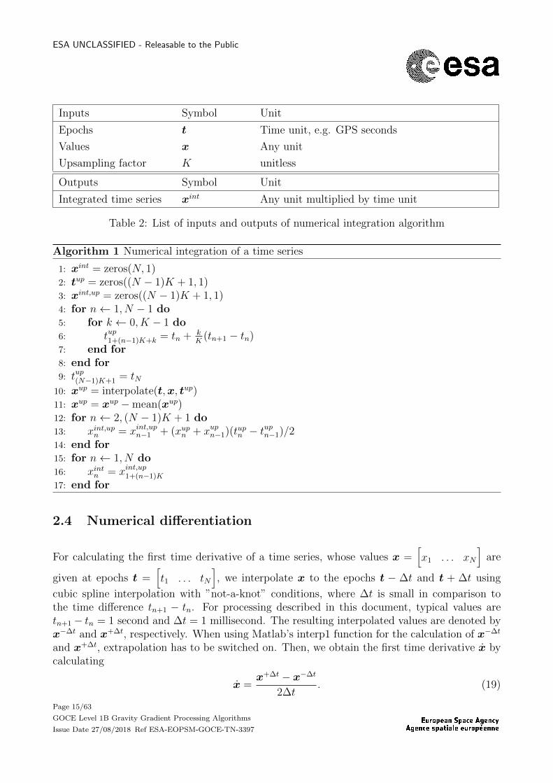
2.3 Numerical integration
For numerical integration of a time series, whose values x =[x1 . . . xN
]are given at epochs
t =[t1 . . . tN
], our approach is interpolating x using cubic spline interpolation with ”not-a-
knot” conditions and then integrating the splines. Since the software available to us does notsupport analytical integration of the splines, we first upsample the time series and then applytrapezoidal integration on the upsampled time series. We denote the epochs and values of theupsampled time series by tup and xup, respectively. We specify the increase of the samplingrate by an integer factor K, such that between each two epochs tn and tn+1 we insert K−1 newepochs that are equally spaced between tn and tn+1. A typical value is K = 20 for processingdescribed in this document. Then, we interpolate the time series x to the epochs tup and reducethe mean from the resulting upsampled time series xup in order to keep the accumulation ofrounding errors low in the following step, which is the trapezoidal integration of xup. Finally,we decimate the integrated time series xup,int to the original epochs to obtain the integratedtime series xint. All of these steps are detailed in Algorithm 1 for numerical integration of atime series. For convenience, we denote the numerical integration by
xint = integrate(t,x, K). (18)
Page 14/63
GOCE Level 1B Gravity Gradient Processing Algorithms
Issue Date 27/08/2018 Ref ESA-EOPSM-GOCE-TN-3397
ESA UNCLASSIFIED - Releasable to the Public
Inputs Symbol Unit
Epochs t Time unit, e.g. GPS seconds
Values x Any unit
Upsampling factor K unitless
Outputs Symbol Unit
Integrated time series xint Any unit multiplied by time unit
Table 2: List of inputs and outputs of numerical integration algorithm
Algorithm 1 Numerical integration of a time series
1: xint = zeros(N, 1)2: tup = zeros((N − 1)K + 1, 1)3: xint,up = zeros((N − 1)K + 1, 1)4: for n← 1, N − 1 do5: for k ← 0, K − 1 do6: tup1+(n−1)K+k = tn + k
K(tn+1 − tn)
7: end for8: end for9: tup(N−1)K+1 = tN10: xup = interpolate(t,x, tup)11: xup = xup −mean(xup)12: for n← 2, (N − 1)K + 1 do13: xint,upn = xint,upn−1 + (xupn + xupn−1)(tupn − t
upn−1)/2
14: end for15: for n← 1, N do16: xintn = xint,up1+(n−1)K
17: end for
2.4 Numerical differentiation
For calculating the first time derivative of a time series, whose values x =[x1 . . . xN
]are
given at epochs t =[t1 . . . tN
], we interpolate x to the epochs t − ∆t and t + ∆t using
cubic spline interpolation with ”not-a-knot” conditions, where ∆t is small in comparison tothe time difference tn+1 − tn. For processing described in this document, typical values aretn+1− tn = 1 second and ∆t = 1 millisecond. The resulting interpolated values are denoted byx−∆t and x+∆t, respectively. When using Matlab’s interp1 function for the calculation of x−∆t
and x+∆t, extrapolation has to be switched on. Then, we obtain the first time derivative x bycalculating
x =x+∆t − x−∆t
2∆t. (19)
Page 15/63
GOCE Level 1B Gravity Gradient Processing Algorithms
Issue Date 27/08/2018 Ref ESA-EOPSM-GOCE-TN-3397

ESA UNCLASSIFIED - Releasable to the Public
The calculation is summarised in Algorithm 2 for numerical differentiation of a time series. Forconvenience, we denote the numerical differentiation by
x = differentiate(t,x,∆t). (20)
Inputs Symbol Unit
Epochs t Time unit, e.g. GPS seconds
Values x Any unit
Upsampling factor ∆t unitless
Outputs Symbol Unit
Integrated time series x Any unit divided by time unit
Table 3: List of inputs and outputs of numerical differentiation algorithm
Algorithm 2 Numerical differentiation of a time series
1: x−∆t = interpolate(t,x, t−∆t)2: x+∆t = interpolate(t,x, t+ ∆t)
3: x = x+∆t−x−∆t
2∆t
Page 16/63
GOCE Level 1B Gravity Gradient Processing Algorithms
Issue Date 27/08/2018 Ref ESA-EOPSM-GOCE-TN-3397
ESA UNCLASSIFIED - Releasable to the Public
3 Convention for rotation matrices, quaternions, and an-
gular rates
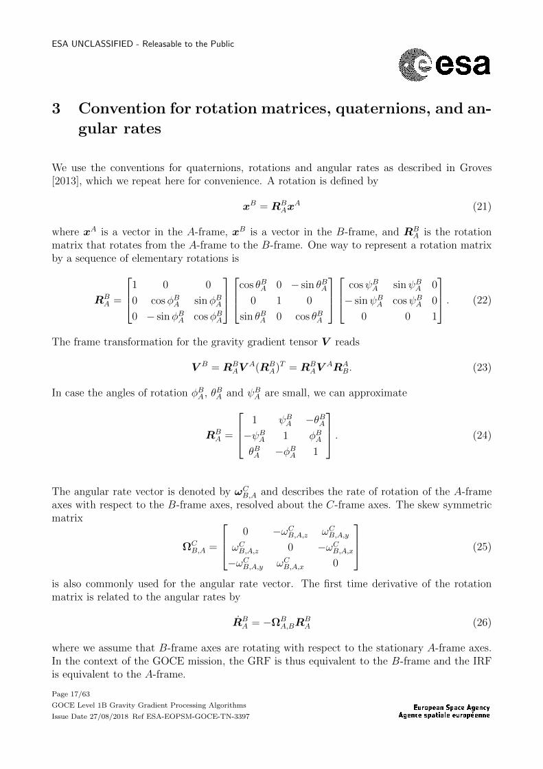
We use the conventions for quaternions, rotations and angular rates as described in Groves[2013], which we repeat here for convenience. A rotation is defined by
xB = RBAx
A (21)
where xA is a vector in the A-frame, xB is a vector in the B-frame, and RBA is the rotation
matrix that rotates from the A-frame to the B-frame. One way to represent a rotation matrixby a sequence of elementary rotations is
RBA =
1 0 0
0 cosφBA sinφBA0 − sinφBA cosφBA
cos θBA 0 − sin θBA
0 1 0
sin θBA 0 cos θBA
cosψBA sinψBA 0
− sinψBA cosψBA 0
0 0 1
. (22)
The frame transformation for the gravity gradient tensor V reads
V B = RBAV
A(RBA)T = RB
AVARA
B. (23)
In case the angles of rotation φBA, θBA and ψBA are small, we can approximate
RBA =
1 ψBA −θBA−ψBA 1 φBAθBA −φBA 1
. (24)
The angular rate vector is denoted by ωCB,A and describes the rate of rotation of the A-frameaxes with respect to the B-frame axes, resolved about the C-frame axes. The skew symmetricmatrix
ΩCB,A =
0 −ωCB,A,z ωCB,A,yωCB,A,z 0 −ωCB,A,x−ωCB,A,y ωCB,A,x 0
(25)
is also commonly used for the angular rate vector. The first time derivative of the rotationmatrix is related to the angular rates by
RBA = −ΩB
A,BRBA (26)
where we assume that B-frame axes are rotating with respect to the stationary A-frame axes.In the context of the GOCE mission, the GRF is thus equivalent to the B-frame and the IRFis equivalent to the A-frame.
Page 17/63
GOCE Level 1B Gravity Gradient Processing Algorithms
Issue Date 27/08/2018 Ref ESA-EOPSM-GOCE-TN-3397

ESA UNCLASSIFIED - Releasable to the Public
In some situation it is more practical to work with quaternions instead of rotation matrices. Aquaternion that describes the same rotation than RB
A is defined as
qBA =[qBA,0 qBA,1 qBA,2 qBA,3
]T(27)
where qBA,0 is the real element of the quaternion and qBA,1, qBA,2 and qBA,3 are imaginary elementsof the quaternions. In the context of the GOCE mission, qBA,0 is labelled qBA,4. The rotationmatrix and the quaternion are related by
RBA =
qBA,02+ qBA,1
2 − qBA,22 − qBA,3
22(qBA,1q
BA,2 + qBA,3q
BA,0) 2(qBA,1q
BA,3 − qBA,2q
BA,0)
2(qBA,1qBA,2 − qBA,3q
BA,0) qBA,0
2 − qBA,12+ qBA,2
2 − qBA,32
2(qBA,2qBA,3 + qBA,1q
BA,0)
2(qBA,1qBA,3 + qBA,2q
BA,0) 2(qBA,2q
BA,3 − qBA,1q
BA,0) qBA,0
2 − qBA,12 − qBA,2
2+ qBA,3
2
. (28)
The sequence of rotations from the A-frame to the C-frame via the B-frame can be performedin terms of rotation matrix multiplications
RCA = RC
BRBA (29)
or equivalently in terms of quaternion multiplications
qCA = qBAqCB , (30)
noting that the sequence of quaternion multiplications is reversed compared to that of rotationmatrix multiplications.
For small rotation angles, we can approximate the quaternion qBA by
qBA =[1 φBA/2 θBA/2 ψBA/2
]T. (31)
For small time intervals ∆t, we can relate the small rotation angles to the angular rates by
qBA(t+ ∆t) = qBA(t)qB(t+∆t)B(t) (32)
where
qB(t+∆t)B(t) =
1
φB(t+∆t)B(t) /2
θB(t+∆t)B(t) /2
ψB(t+∆t)B(t) /2
=
1∫ t+∆t
tωBA,B,xdt/2∫ t+∆t
tωBA,B,ydt/2∫ t+∆t
tωBA,B,zdt/2
. (33)
Equation (26) expressed in terms of quaternions reads
qBA = qBAWBA,B (34)
where the product WBA,Bq
BA is a quaternion multiplication and
WBA,B =
[0 ωBA,B,x/2 ωBA,B,y/2 ωBA,B,z/2
]T(35)
is a vector that contains the angular rates. Note that the different sign in Eq. (34) with respectto Eq. (26) results from the different signs in Eq. (24) and Eq. (25).
Page 18/63
GOCE Level 1B Gravity Gradient Processing Algorithms
Issue Date 27/08/2018 Ref ESA-EOPSM-GOCE-TN-3397

ESA UNCLASSIFIED - Releasable to the Public
Algorithm 3 Converting rotation matrices to quaternions
1: t = R11 +R22 +R33
2: if t > 0 then3: r =
√1 + t
4: s = 0.5/r5: q0 = 0.5r6: q1 = (R32 −R23)s7: q2 = (R13 −R31)s8: q3 = (R21 −R12)s9: else if R11 > R22 and R11 > R33 then10: r =
√1 +R11 −R22 −R33
11: s = 0.5/r12: q0 = (R32 −R23)s13: q1 = 0.5r14: q2 = (R12 +R21)s15: q3 = (R31 +R13)s16: else if R22 > R11 and R22 > R33 then17: r =
√1 +R22 −R11 −R33
18: s = 0.5/r19: q0 = (R13 −R31)s20: q1 = (R21 +R12)s21: q2 = 0.5r22: q3 = (R32 +R23)s23: else . R33 > R11 and R33 > R22
24: r =√
1 +R33 −R11 −R22
25: s = 0.5/r26: q0 = (R21 −R12)s27: q1 = (R31 +R13)s28: q2 = (R32 +R23)s29: q3 = 0.5r30: end if
Page 19/63
GOCE Level 1B Gravity Gradient Processing Algorithms
Issue Date 27/08/2018 Ref ESA-EOPSM-GOCE-TN-3397

ESA UNCLASSIFIED - Releasable to the Public
Page 20/63
GOCE Level 1B Gravity Gradient Processing Algorithms
Issue Date 27/08/2018 Ref ESA-EOPSM-GOCE-TN-3397

ESA UNCLASSIFIED - Releasable to the Public
4 Star tracker data processing
4.1 Star tracker data preprocessing
On board the GOCE satellite are three star trackers, each providing its orientation with respectto the international celestial reference frame (IRF). The orientation is provided in form of anattitude quaternion qSRFi
IRF , where i ∈ 1, 2, 3 indicates the star tracker. The star trackers alsoprovide various flags that give information on the tracking status. In the first step of the startracker data preprocessing, we use the validity flag fV ALi
and the big-bright-object flag fBBOi,
which indicate whether the star tracker is providing a valid attitude and whether a big andbright object is within the field-of-view, respectively. We discard all attitude quaternions thatare flagged invalid, i.e. fV ALi
= 0 and for which a big-bright-object is detected, i.e. fBBOi= 1.
Since the measurements of the star trackers are not synchronised with the gradiometer measure-ments, we resample all star tracker data to the measurement epochs of the gradiometer. Thefirst step is loading the star tracker epochs, quaternions and flags from the STR VC3 1B andSTR VC3 1B files and star tracker CCD temperatures from the AUX NOM 1B files, followedby sorting all loaded data into individual variables for each star tracker. Then, we amend foreach star tracker all quaternion sign flips between subsequent epochs using Algorithm 4, notingthat qSRFi
IRF and −qSRFiIRF describe the same attitude. For the resampling we select all quaternions
in a time window [tG,n −∆tq, tG,n + ∆tq] centred around the gradiometer epochs tG,n and ap-proximate them with a quadratic function, provided that we have at least three quaternionswithin the time window and at least one quaternion on each side of tG,n. We use the sameapproach to resample the star tracker CCD temperatures to the gradiometer epochs, with thedifferences that we use a larger time window [tG,n −∆tT , tG,n + ∆tT ] and that we approximatethe temperatures by their mean value within the time window. These processing steps consti-tute the star tracker preprocessing, which is detailed in Algorithm 5. Typical values for thetime windows are ∆tq = 1.75 seconds, i.e. up to 7 star tracker epochs due to the sampling rateof 2 Hz for quaternions, and ∆tT = 300 seconds, i.e. up to 38 epochs due to the sampling rateof 1/16 Hz for temperatures. Further, it is noted that the resolution for the temperatures islimited to roughly 0.5C.
4.2 Star tracker data combination
We use the approach of Romans [2003] for the combination of the attitude quaternions. It isbased on a least squares adjustment of the star tracker quaternions, in which the pointing of thestar tracker bore sight is assumed to be 10 times more accurate compared to the rotation aroundthe bore sight. It requires knowledge of the orientation of the star trackers in the commonreference frame (CRF), which is aligned with the satellite’s body axes. That orientation is aavailable in form the rotation matrices RCRF
SRF1, RCRF
SRF2and RCRF
SRF3defined in Eqs. (36–38). Our
Page 21/63
GOCE Level 1B Gravity Gradient Processing Algorithms
Issue Date 27/08/2018 Ref ESA-EOPSM-GOCE-TN-3397

ESA UNCLASSIFIED - Releasable to the Public
addition to the approach of Romans [2003] is the correction of relative biases between the startrackers, which are modelled as linear functions of the temperature as defined in Eqs. (39–44).Algorithm 6 shows all processing steps of the star tracker combination in detail.
RCRFSRF1
=
0.999991953964000 −0.003855453067860 0.001107921250810
−0.002875276132160 −0.496285685373000 0.868154508875000
−0.002797283507320 −0.868150709252000 −0.496292777733000
(36)
RCRFSRF2
=
0.999868439135000 0.015726793513000 −0.003971446564830
0.016149312081100 −0.942268716879000 0.334468032720000
0.001517939828470 −0.334488165946000 −0.942398728087000
(37)
RCRFSRF3
=
0.011846242780200 −0.769183928773000 0.638917639645000
−0.491411293086000 0.551999304112000 0.673655482637000
−0.870847063243000 −0.321951629871000 −0.371446551289000
(38)
bCRFS1(TS1) = bCRFC1
+ TS1 bCRFT1
(39)
bCRFC1= 10−3
0.116219900793661
−0.134723547186391
−0.029472128350279
, bCRFT1= 10−5
0.278591682091328
−0.118889821498250
−0.140330884420176
(40)
bCRFS2(TS2) = bCRFC2
+ TS2 bCRFT2
(41)
bCRFC2= 10−3
0.087909010253279
−0.223645453432216
−0.007718724727271
, bCRFT2= 10−5
0.046609082258701
0.226425836947881
−0.096374884840557
(42)
bCRFS3(TS3) = bCRFC3
+ TS3 bCRFT3
(43)
bCRFC3= 10−3
0.111289309287413
−0.147455472014728
0.021704225770305
, bCRFT3= 10−5
0.053953847437714
−0.064274246885287
0.379499278972736
(44)
Page 22/63
GOCE Level 1B Gravity Gradient Processing Algorithms
Issue Date 27/08/2018 Ref ESA-EOPSM-GOCE-TN-3397

ESA UNCLASSIFIED - Releasable to the Public
Inputs Symbol Unit Contents
Flags f unitless 0 = invalid, 1 = valid
Quaternions q unitless Quaternions with sign flips
Outputs Symbol Unit Contents
Quaternions q unitless Quaternions without sign flips
Table 4: List of inputs and outputs of algorithm for making quaternions continuous
Algorithm 4 Making quaternions continuous
1: for n← 2, N do2: if fn == 0 then . No valid attitude available3: qn = qn−1
4: else if qTn qn−1 < 0 then5: qn = −qn6: end if7: end for
Page 23/63
GOCE Level 1B Gravity Gradient Processing Algorithms
Issue Date 27/08/2018 Ref ESA-EOPSM-GOCE-TN-3397

ESA UNCLASSIFIED - Releasable to the Public
Inputs Symbol Unit Contents
Epochs tG GPS seconds Epochs of gradiometer
Epochs tS1 , tS2 , tS3 GPS secondsEpochs of attitude of three startrackers
Attitudequaternions
qIRFSRF1, qIRFSRF2
, qIRFSRF3unitless
Orientation of star tracker inIRF
Flags fBBO1 , fBBO2 , fBBO3 unitless
Big-bright-object (BBO) flag ofstar trackers: 1 = BBO in fieldof view, 0 = no BBO in field ofview
Flags fV AL1 , fV AL2 , fV AL3 unitlessValid flag of star trackers: 1 =valid attitude, 0 = invalid atti-tude
Epochs tT1 , tT2 , tT3 GPS secondsEpochs of temperature of threestar trackers
Temperatures TS1 , TS2 , TS3oC
Temperature of three startrackers
Half windowwidth
∆tq secondsWindow width for selection ofquaternions
Half windowwidth
∆tT secondsWindow width for selection oftemperatures
Outputs Symbol Unit Contents
Attitudequaternions
qIRF,resSRF1, qIRF,resSRF1
, qIRF,resSRF1unitless
Orientation of SRF1, SRF2,SRF3 wrt. IRF resampled togradiometer epochs
Temperatures T resS1
, T resS2
, T resS3
oCTemperature of three startrackers resampled to gra-diometer epochs
Flags f resS1, f resS2
, f resS3unitless
Flags of resampled star trackerdata: 1 = usable, 0 = not us-able
Table 5: List of inputs and outputs of star tracker preprocessing algorithm
Page 24/63
GOCE Level 1B Gravity Gradient Processing Algorithms
Issue Date 27/08/2018 Ref ESA-EOPSM-GOCE-TN-3397
ESA UNCLASSIFIED - Releasable to the Public
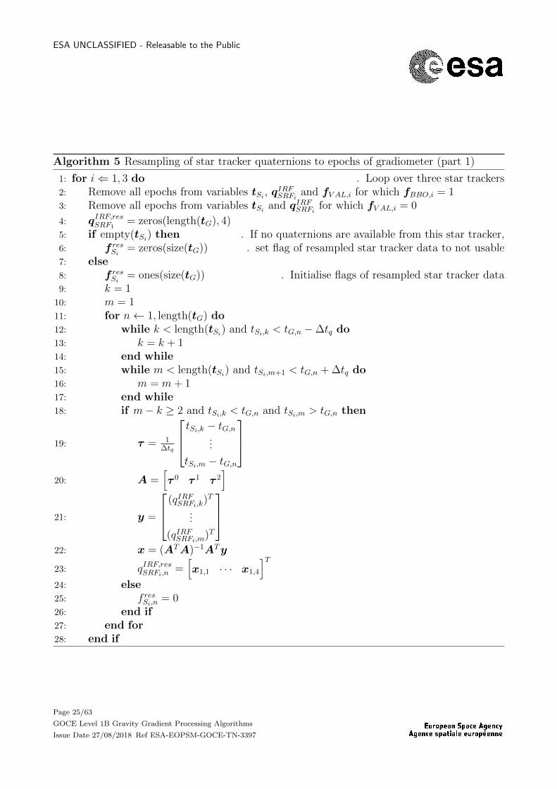
Algorithm 5 Resampling of star tracker quaternions to epochs of gradiometer (part 1)
1: for i⇐ 1, 3 do . Loop over three star trackers2: Remove all epochs from variables tSi
, qIRFSRFiand fV AL,i for which fBBO,i = 1
3: Remove all epochs from variables tSiand qIRFSRFi
for which fV AL,i = 0
4: qIRF,resSRF1= zeros(length(tG), 4)
5: if empty(tSi) then . If no quaternions are available from this star tracker,
6: f resSi= zeros(size(tG)) . set flag of resampled star tracker data to not usable
7: else8: f resSi
= ones(size(tG)) . Initialise flags of resampled star tracker data9: k = 110: m = 111: for n← 1, length(tG) do12: while k < length(tSi
) and tSi,k < tG,n −∆tq do13: k = k + 114: end while15: while m < length(tSi
) and tSi,m+1 < tG,n + ∆tq do16: m = m+ 117: end while18: if m− k ≥ 2 and tSi,k < tG,n and tSi,m > tG,n then
19: τ = 1∆tq
tSi,k − tG,n...
tSi,m − tG,n
20: A =
[τ 0 τ 1 τ 2
]21: y =
(qIRFSRFi,k)T
...
(qIRFSRFi,m)T
22: x = (ATA)−1ATy
23: qIRF,resSRFi,n=[x1,1 · · · x1,4
]T24: else25: f resSi,n
= 026: end if27: end for28: end if
Page 25/63
GOCE Level 1B Gravity Gradient Processing Algorithms
Issue Date 27/08/2018 Ref ESA-EOPSM-GOCE-TN-3397
ESA UNCLASSIFIED - Releasable to the Public
Algorithm 5 Resampling of star tracker quaternions to epochs of gradiometer (part 2)
29: TSi= zeros(length(tG), 1)
30: if empty(tTi) then . If no temperatures are available from this star tracker,31: f resSi
= zeros(size(tG)) . set flag of resampled star tracker data to not usable32: else33: k = 134: m = 135: for n← 1, length(tG) do36: while k < length(tTi) and tTi,k < tG,n −∆tT do37: k = k + 138: end while39: while m < length(tTi) and tTi,m+1 < tG,n + ∆tT do40: m = m+ 141: end while42: if m− k ≥ 2 and tTi,k < tG,n and tTi,m > tG,n then
43: T resSi,n= mean(
[TSi,k · · · TSi,m
])
44: else45: f resSi,n
= 046: end if47: end for48: end if49: end for
Page 26/63
GOCE Level 1B Gravity Gradient Processing Algorithms
Issue Date 27/08/2018 Ref ESA-EOPSM-GOCE-TN-3397

ESA UNCLASSIFIED - Releasable to the Public
Inputs Symbol Unit Contents Source algorithm
Attitudequaternions
qIRF,resSRF1, qIRF,resSRF2
, qIRF,resSRF3unitless
Resampled orien-tation of SRF1,SRF2, SRF3 wrt.IRF
Star tracker pre-processing
Flag f resS1,n, f resS2,n
, f resS3,nunitless
Flag of resam-pled star trackerquaternion: 1 =valid, 0 = invalid
Star tracker pre-processing
Temperature T resS1,n
, T resS2,n
, T resS3,n
oCResampled tem-perature of startrackers
Star tracker pre-processing
Constants Symbol Unit Contents Source
Biases bCRFS1, bCRFS2
, bCRFS3unitless
Star tracker atti-tude bias in CRF
Star tracker cali-bration
Rotation RCRFSRF1
, RCRFSRF2
, RCRFSRF3
unitlessStar tracker orien-tation in CRF
Outputs Symbol Unit Contents
Attitudequaternions
qIRFCRF unitlessOrientation ofCRF wrt. IRF
Flags f unitless1 = valid, 0 = in-valid
Square-sum ofresiduals
Ω rad2 Square-sum ofresiduals
Cofactor ma-trices
Q1, Q2, Q3, Q12, Q13,Q23, Q123
unitless Cofactor matrices
Table 6: List of inputs and outputs of star tracker combination algorithm
Page 27/63
GOCE Level 1B Gravity Gradient Processing Algorithms
Issue Date 27/08/2018 Ref ESA-EOPSM-GOCE-TN-3397

ESA UNCLASSIFIED - Releasable to the Public
Algorithm 6 Star tracker combination (part 1)
1: P SRF =
1 0 0
0 1 0
0 0 1102
. attitude around boresight axis 10 times worse than others
2: P CRF1 = RCRF
SRF1∗ P SRF ∗ (RCRF
SRF1)T
3: P CRF2 = RCRF
SRF2∗ P SRF ∗ (RCRF
SRF2)T
4: P CRF3 = RCRF
SRF3∗ P SRF ∗ (RCRF
SRF3)T
5: Convert RSRF1CRF to qSRF1
CRF using Algorithm 36: Convert RSRF2
CRF to qSRF2CRF using Algorithm 3
7: Convert RSRF3CRF to qSRF3
CRF using Algorithm 38: eCRF1 = zeros(N, 3)9: eCRF2 = zeros(N, 3)10: eCRF3 = zeros(N, 3)11: qIRFCRF = zeros(N, 4)12: for n← 1, N do13: bCRFS1,n
= bCRFC1+ T resS1,n
bCRFT1
14: bCRFS2,n= bCRFC2
+ T resS2,nbCRFT2
15: bCRFS3,n= bCRFC3
+ T resS3,nbCRFT3
16: bSRF1S1,n
= RSRF1CRF b
CRFS1,n
17: bSRF2S2,n
= RSRF2CRF b
CRFS2,n
18: bSRF3S3,n
= RSRF3CRF b
CRFS3,n
19: q12,n = (qIRF,resSRF1,nqSRF1CRF )∗(qIRF,resSRF2,n
qSRF2CRF ) . quaternion multiplication/conjugation
20: q13,n = (qIRF,resSRF1,nqSRF1CRF )∗(qIRF,resSRF3,n
qSRF3CRF ) . quaternion multiplication/conjugation
21: q23,n = (qIRF,resSRF2,nqSRF2CRF )∗(qIRF,resSRF3,n
qSRF3CRF ) . quaternion multiplication/conjugation
22: d12,n = 2 ∗ sign q12,n,0
q12,n,1
q12,n,2
q12,n,3
+ bCRFS1,n− bCRFS2,n
23: d13,n = 2 ∗ sign q13,n,0
q13,n,1
q13,n,2
q13,n,3
+ bCRFS1,n− bCRFS3,n
24: d23,n = 2 ∗ sign q23,n,0
q23,n,1
q23,n,2
q23,n,3
+ bCRFS2,n− bCRFS3,n
25: end for
Page 28/63
GOCE Level 1B Gravity Gradient Processing Algorithms
Issue Date 27/08/2018 Ref ESA-EOPSM-GOCE-TN-3397
ESA UNCLASSIFIED - Releasable to the Public
Algorithm 6 Star tracker combination (part 2)
26: for n← 1, N do27: if f resS1,n
= 1 and f res2,n = 1 and f res3,n = 0 then28: eCRF1,n = −(P CRF
1 + P CRF2 )−1P CRF
2 d12,n
29: eCRF2,n = eCRF1,n + d12,n
30: end if31: if f res1,n = 1 and f res2,n = 0 and f res3,n = 1 then32: eCRF1,n = −(P CRF
1 + P CRF3 )−1P CRF
3 d13,n
33: eCRF3,n = eCRF1,n + d13,n
34: end if35: if f res1,n = 0 and f res2,n = 1 and f res3,n = 1 then36: eCRF2,n = −(P CRF
2 + P CRF3 )−1P CRF
3 d23,n
37: eCRF3,n = eCRF2,n + d23,n
38: end if39: if f res1,n = 1 and f res2,n = 1 and f res3,n = 1 then40: eCRF1,n = −(P CRF
1 + P CRF2 + P CRF
3 )−1(P CRF2 d12,n + P CRF
3 d13,n)41: eCRF2,n = eCRF1,n + d12,n
42: eCRF3,n = eCRF1,n + d13,n
43: end if44: if f resS1,n
= 1 or f resS2,n= 1 or f resS3,n
= 1 then . set flag of combined quaternion45: fn = 146: else47: fn = 048: end if49: if f resS1,n
= 1 then
50: qIRFCRF,n = (qIRFSRF1,n
[1
−(eSRF11,n + bSRF1
1,n )/2
])qSRF1CRF . quat. multiplications
51: end if52: if f resS2,n
= 1 then
53: qIRFCRF,n = (qIRFSRF2,n
[1
−(eSRF22,n + bSRF2
2,n )/2
])qSRF2CRF . quat. multiplications
54: end if55: if f resS3,n
= 1 then
56: qIRFCRF,n = (qIRFSRF3,n
[1
−(eSRF33,n + bSRF3
3,n )/2
])qSRF3CRF . quat. multiplications
57: end if
58: qIRFCRF,n =qIRFCRF,n
|qIRFCRF,n|
. normalize quaternion
59: end for
Page 29/63
GOCE Level 1B Gravity Gradient Processing Algorithms
Issue Date 27/08/2018 Ref ESA-EOPSM-GOCE-TN-3397
ESA UNCLASSIFIED - Releasable to the Public
Algorithm 6 Star tracker combination (part 3, optional)
60: RSRF = chol(P SRF ) . Cholesky factorization61: Ω = 0 . square-sum of residuals62: for n← 1, N do63: eSRF1
1,n = RSRF1CRF e
CRF1,n
64: eSRF22,n = RSRF2
CRF eCRF2,n
65: eSRF33,n = RSRF3
CRF eCRF3,n
66: Ω = Ω + (RSRFeSRF11,n )T (RSRFeSRF1
1,n )
67: Ω = Ω + (RSRFeSRF22,n )T (RSRFeSRF2
2,n )
68: Ω = Ω + (RSRFeSRF33,n )T (RSRFeSRF3
3,n )69: end for70: Q1 = (P CRF
1 )−1 . cofactor matrix71: Q2 = (P CRF
2 )−1 . cofactor matrix72: Q3 = (P CRF
3 )−1 . cofactor matrix73: Q12 = (P CRF
1 + P CRF2 )−1 . cofactor matrix
74: Q13 = (P CRF1 + P CRF
3 )−1 . cofactor matrix75: Q23 = (P CRF
2 + P CRF3 )−1 . cofactor matrix
76: Q123 = (P CRF1 + P CRF
2 + P CRF3 )−1 . cofactor matrix
Page 30/63
GOCE Level 1B Gravity Gradient Processing Algorithms
Issue Date 27/08/2018 Ref ESA-EOPSM-GOCE-TN-3397
ESA UNCLASSIFIED - Releasable to the Public
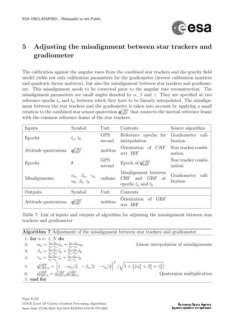
5 Adjusting the misalignment between star trackers and
gradiometer
The calibration against the angular rates from the combined star trackers and the gravity fieldmodel yields not only calibration parameters for the gradiometer (inverse calibration matricesand quadratic factor matrices), but also the misalignment between star trackers and gradiome-ter. This misalignment needs to be corrected prior to the angular rate reconstruction. Themisalignment parameters are small angles denoted by α, β and γ. They are specified at tworeference epochs ta and tb, between which they have to be linearly interpolated. The misalign-ment between the star trackers and the gradiometer is taken into account by applying a smallrotation to the combined star sensor quaternion qCRFIRF that connects the inertial reference framewith the common reference frame of the star trackers.
Inputs Symbol Unit Contents Source algorithm
Epochs ta, tbGPSsecond
Reference epochs forinterpolation
Gradiometer cali-bration
Attitude quaternions qCRFIRF unitlessOrientation of CRFwrt. IRF
Star tracker combi-nation
Epochs tGPSsecond
Epoch of qCRFIRF
Star tracker combi-nation
Misalignmentsαa, βa, γa,αb, βb, γb
radiansMisalignment betweenCRF and GRF atepochs ta and tb
Gradiometer cali-bration
Outputs Symbol Unit Contents
Attitude quaternions qGRFIRF unitlessOrientation of GRFwrt. IRF
Table 7: List of inputs and outputs of algorithm for adjusting the misalignment between startrackers and gradiometer
Algorithm 7 Adjustment of the misalignment between star trackers and gradiometer
1: for n← 1, N do2: αn = tb−tn
tb−taαa + tn−ta
tb−taαb . Linear interpolation of misalignments
3: βn = tb−tntb−ta
βa + tn−tatb−ta
βb4: γn = tb−tn
tb−taγa + tn−ta
tb−taγb
5: qGRFCRF,n =[1 −αn/2 −βn/2 −γn/2
]T/√
1 + 14(α2
n + β2n + γ2
n)
6: qGRFIRF,n = qCRFIRF,nqGRFCRF,n . Quaternion multiplication
7: end for
Page 31/63
GOCE Level 1B Gravity Gradient Processing Algorithms
Issue Date 27/08/2018 Ref ESA-EOPSM-GOCE-TN-3397

ESA UNCLASSIFIED - Releasable to the Public
Page 32/63
GOCE Level 1B Gravity Gradient Processing Algorithms
Issue Date 27/08/2018 Ref ESA-EOPSM-GOCE-TN-3397
ESA UNCLASSIFIED - Releasable to the Public
6 Accelerometer data processing
6.1 Accelerometer data calibration
The relationship of the measured and true acceleration is defined by the quadratic function
ai = bi +Miai +Kia2i +Wiω + ni (45)
where ai is the measured acceleration, bi is the bias of the measured acceleration, Mi is acalibration matrix for the i-th accelerometer, ai is the true acceleration, Ki is the quadraticfactor matrix,Wi is the angular acceleration coupling matrix, ω is the true angular acceleration,and ni is noise in the measured acceleration. It should be noted that Mi is a general 3 × 3matrix and Ki is a 3 × 3 diagonal matrix. The elements of Wi depend on the onboard proofmass control and are defined as
Wi =
0 0 0
ei 0 gi
0 fi 0
for i ∈ 1, 4, (46)
Wi =
0 0 gi
0 0 0
ei fi 0
for i ∈ 2, 5 (47)
and
Wi =
0 fi 0
ei 0 gi
0 0 0
for i ∈ 3, 6. (48)
For the square of a vector as in a2i , we use the convention that the elements of the vector are
squared, i.e.
a2i =
a2ix
a2iy
a2iz
. (49)
Differential and common mode acceleration are defined by[adij
acij
]=
1
2
[ai − ajai + aj
]. (50)
When defining the inverse calibration matrix as
Mij = 2
[Mi +Mj Mi −Mj
Mi −Mj Mi +Mj
]−1
, (51)
Page 33/63
GOCE Level 1B Gravity Gradient Processing Algorithms
Issue Date 27/08/2018 Ref ESA-EOPSM-GOCE-TN-3397
ESA UNCLASSIFIED - Releasable to the Public
we can reformulate Eq. (45) to[adij
acij
]=
[bdij
bcij
]+M−1
ij
[adij
acij
]+
1
2
[Ki −Kj
Ki Kj
][a2i
a2j
]+
[Wdij
Wcij
]ω +
[ndij
ncij
], (52)
where all differential and common terms are signified by subscripts d and c, respectively, anddefined analogously to Eq. (50).
A so-called satellite shaking procedure yields a first estimate of the inverse calibration matrixMij, which we denote by Mij. Applying the first estimate of the inverse calibration matrix tothe measured acceleration yields [
adij
acij
]= Mij
[adij
acij
], (53)
where adij and acij are calibrated differential and common mode acceleration, respectively, ofthe first stage of the calibration. We regard adij and acij as good approximations of adij andacij, respectively, which will be refined in the second stage of the calibration.
Inserting Eq. (53) into Eq. (52) gives[adij
acij
]=
[bdij
bcij
]+MijM
−1ij
[adij
acij
]+
1
2Mij
[Ki −Kj
Ki Kj
][a2i
a2j
]+Mij
[Wdij
Wcij
]ω+
[ndij
ncij
], (54)
where bdij, bcij, ndij, and ncij are defined analogously to Eq. (53). In order to proceed, we needto find approximations for a2
i and a2j . For this purpose, we assume that quadratic factors and
angular acceleration couplings are small, i.e. Ki ≈ 0, Kj ≈ 0, Wdij ≈ 0 and Wcij ≈ 0, theinverse calibration matrix estimated in the satellite shaking procedure approximates the trueinverse calibration matrix well, i.e. Mij ≈Mij, and that we can neglect the noise terms, i.e.ndij ≈ 0 and ncij ≈ 0. With these assumptions, Eq. (54) reduces to[
adij
acij
]=
[bdij
bcij
]+
[adij
acij
], (55)
which leads to [a2i
a2j
]=
[(ai − bi)2
(aj − bj)2
]=
[a2i
a2j
]− 2
[aibi
aj bj
]+
[b2i
b2j
]. (56)
Inserting this result for a2i and a2
j into Eq. (54) gives[adij
acij
]=
[bdij
bcij
]+ MijM
−1ij
[adij
acij
]
+1
2Mij
[Ki −Kj
Ki Kj
]([a2i
a2j
]− 2
[aibi
aj bj
]+
[b2i
b2j
])+ Mij
[Wdij
Wcij
]ω +
[ndij
ncij
]. (57)
Page 34/63
GOCE Level 1B Gravity Gradient Processing Algorithms
Issue Date 27/08/2018 Ref ESA-EOPSM-GOCE-TN-3397

ESA UNCLASSIFIED - Releasable to the Public
In order to simplify the equation, we note that[Ki −Kj
Ki Kj
][aibi
aj bj
]=
[Kibi −Kj bj
Kibi Kj bj
][ai
aj
](58)
=
[Kibi −Kj bj
Kibi Kj bj
][acij + adij
acij − adij
](59)
=
[Kibi +Kj bj Kibi −Kj bj
Kibi −Kj bj Kibi +Kj bj
][adij
acij
], (60)
which leads to[adij
acij
]=
[bdij
bcij
]+
1
2Mij
[Ki −Kj
Ki Kj
][b2i
b2j
]+ MijM
−1ij
[adij
acij
]
− Mij
[Kibi +Kj bj Kibi −Kj bj
Kibi −Kj bj Kibi +Kj bj
][adij
acij
]
+1
2Mij
[Ki −Kj
Ki Kj
][a2i
a2j
]+ Mij
[Wdij
Wcij
]ω +
[ndij
ncij
]. (61)
We solve this equation for adij and acij, which gives[adij
acij
]= −MijM
−1ij
([bdij
bcij
]+
1
2Mij
[Ki −Kj
Ki Kj
][b2i
b2j
])
+Mij
(M−1
ij +
[Kibi +Kj bj Kibi −Kj bj
Kibi −Kj bj Kibi +Kj bj
])[adij
acij
]
− 1
2Mij
[Ki −Kj
Ki Kj
][a2i
a2j
]−Mij
[Wdij
Wcij
]ω −MijM
−1ij
[ndij
ncij
]. (62)
This equation shows that adij and acij are a quadratic function of adij and acij plus a linearfunction of ω. We rewrite the equation as[
adij
acij
]=
[¯bdij¯bcij
]+ Mij
[adij
acij
]+ Kij
[a2i
a2j
]+ Wijω +
[¯ndij¯ncij
](63)
where [¯bdij¯bcij
]= −MijM
−1ij
([bdij
bcij
]+
1
2Mij
[Ki −Kj
Ki Kj
][b2i
b2j
]), (64)
Mij = Mij
(M−1
ij +
[Kibi +Kj bj Kibi −Kj bj
Kibi −Kj bj Kibi +Kj bj
]), (65)
Page 35/63
GOCE Level 1B Gravity Gradient Processing Algorithms
Issue Date 27/08/2018 Ref ESA-EOPSM-GOCE-TN-3397

ESA UNCLASSIFIED - Releasable to the Public
Kij = −1
2Mij
[Ki −Kj
Ki Kj
]≈ −1
2
[Ki −Kj
Ki Kj
]. (66)
and
Wij = −Mij
[Wdij
Wcij
]≈ −
[Wdij
Wcij
]. (67)
The matrices Mij, Kij and Wij are determined in the calibration against the combined startracker angular rates and a gravity field model. It should be noted that the diagonal elementsof Mij are coupled to the accelerometer biases through the quadratic factors, which is a conse-quence of using the biased acceleration measurements as proxy for the true acceleration. Sincethe biases are drifting over time, we should expect that the diagonal elements of each 3 × 3submatrix of Mij drift in the same way.
Noting that we have to estimate Mij, Kij and Wij because the true inverse calibration matrixMij is unknown, we replace adij and acij by ¯adij and ¯acij, respectively, in order to signify thatwe obtain not the true acceleration, and find the calibrated acceleration[
¯adij¯acij
]=
[¯bdij¯bcij
]+ Mij
[adij
acij
]+ Kij
[(acij + adij)
2
(acij − adij)2
]+ Wijω +
[¯ndij¯ncij
]. (68)
The equation contains the true angular acceleration ω, which is also unknown. We use theangular acceleration ˙ω as a proxy, which is calculated using Algorithm 14 using as input thecombined star tracker quaternions, which are an output of Algorithm 6, and the gradiometerangular accelerations that are calculated from adij and acij according to Algorithm 12. Wethus exchange ω by ˙ω in Eq.(69) and obtain
[¯adij¯acij
]=
[¯bdij¯bcij
]+ Mij
[adij
acij
]+ Kij
[(acij + adij)
2
(acij − adij)2
]+ Wij ˙ω +
[¯ndij¯ncij
]. (69)
Now that we derived the equations for the calibration in detail, we can summarise the algorithmfor the gradiometer calibration as follows. In the first stage, we use Eq. (53) to apply the inversecalibration matrices determined in the satellite shaking procedure. In the second stage, we useEq. (69) to apply the calibration matrices Mij, Kij and Wij, which are determined in anadvanced calibration procedure from science mode and shaking mode data. In both stages, welinearly interpolate the calibration matrices in order to account for small drifts in the calibrationparameters. The matrices Mij are interpolated between two reference epochs ta and tb andthe matrices Mij, Kij and Wij are interpolated between two reference epochs ta and tb. Thereference epochs ta and tb refer to the dates of satellite shaking procedures, whereas ta and tbare manually selected based on reported onboard events and observed data quality, i.e. thetime intervals [ta, tb] and [ta, tb] are not necessarily the same.
Page 36/63
GOCE Level 1B Gravity Gradient Processing Algorithms
Issue Date 27/08/2018 Ref ESA-EOPSM-GOCE-TN-3397

ESA UNCLASSIFIED - Releasable to the Public
Inputs Symbol Unit Contents Source algorithm
Epochs ta, tb sReferences epochsin GPS seconds
Satellite shakingprocedure
Accelerationad14, ac14, ad25,ac25, ad36, ac36
m/s2
Measured commonand differentialmode acceleration
EGG NOM 1b
Inverse calibrationmatrices
M14a, M25a,M36a, M14b,M25b, M36b
unitlessInverse calibrationmatrices at epochsta nd tb
Satellite shakingprocedure
Outputs Symbol Unit Contents
Accelerationad14, ac14, ad25,ac25, ad36, ac36
m/s2
Shaking mode cal-ibrated commonand differentialmode acceleration
Table 8: List of inputs and outputs of the gradiometer calibration algorithm (satellite shaking)
Algorithm 8 Gradiometer calibration (satellite shaking)
1: for n← na, nb do
2:
[ad14n
ac14n
]=(tb−tntb−ta
M14a + tn−tatb−ta
M14b
)[ad14n
ac14n
]
3:
[ad25n
ac25n
]=(tb−tntb−ta
M25a + tn−tatb−ta
M25b
)[ad25n
ac25n
]
4:
[ad36n
ac36n
]=(tb−tntb−ta
M36a + tn−tatb−ta
M36b
)[ad36n
ac36n
]5: end for
6.2 Gross outlier detection and removal
It is advisable to remove gross outliers prior to the angular rate reconstruction since theireffects would be ”smeared out” in the angular rate and acceleration reconstruction that involvesnumerical integration and filtering. We employ the following simple algorithm for detecting andremoving gross outliers. The algorithm relies on the fact that moving-median filters are (a)robust against outliers, spikes, etc. (b) preserve edges and step functions, and (c) behave likelow-pass filters. A symmetric moving median filter is defined by
yn = median(xn−k, xn−k+1, . . . xn+k) (70)
Page 37/63
GOCE Level 1B Gravity Gradient Processing Algorithms
Issue Date 27/08/2018 Ref ESA-EOPSM-GOCE-TN-3397

ESA UNCLASSIFIED - Releasable to the Public
Algorithm 9 Gradiometer calibration (science mode)
1: for n← na, nb do
2:
[¯ad14n
¯ac14n
]=(tb−tntb−ta
M14a + tn−tatb−ta
M14b
)[ad14n
ac14n
]
3:
[¯ad25n
¯ac25n
]=(tb−tntb−ta
M25a + tn−tatb−ta
M25b
)[ad25n
ac25n
]
4:
[¯ad36n
¯ac36n
]=(tb−tntb−ta
M36a + tn−tatb−ta
M36b
)[ad36n
ac36n
]
5:
[¯ad14n
¯ac14n
]=
[¯ad14n
¯ac14n
]+(tb−tntb−ta
K14a + tn−tatb−ta
K14b
)[(ac14n + ad14n)2
(ac14n − ad14n)2
]
6:
[¯ad25n
¯ac25n
]=
[¯ad25n
¯ac25n
]+(tb−tntb−ta
K25a + tn−tatb−ta
K25b
)[(ac25n + ad25n)2
(ac25n − ad25n)2
]
7:
[¯ad36n
¯ac36n
]=
[¯ad36n
¯ac36n
]+(tb−tntb−ta
K36a + tn−tatb−ta
K36b
)[(ac36n + ad36n)2
(ac36n − ad36n)2
]
8:
[¯ad14n
¯ac14n
]=
[¯ad14n
¯ac14n
]+(tb−tntb−ta
W14a + tn−tatb−ta
W14b
)˙ω
9:
[¯ad25n
¯ac25n
]=
[¯ad25n
¯ac25n
]+(tb−tntb−ta
W25a + tn−tatb−ta
W25b
)˙ω
10:
[¯ad36n
¯ac36n
]=
[¯ad36n
¯ac36n
]+(tb−tntb−ta
W36a + tn−tatb−ta
W36b
)˙ω
11: end for
where xn is the filter input, yn is the filter output, and 2k + 1 is the width of the movingwindow. When subtracting the filter output from the filter input, i.e.
en = xn −median(xn−k, xn−k+1, . . . xn+k), (71)
the residuals en should contain mainly high-frequency noise and features like outliers, spikes,etc. When the width of the moving window is chosen appropriately, the outliers, spikes, etc.will not be ”smeared out”, as would be the case for a moving-average filter, which makes iteasy to detect them.
An outlier is detected, if the absolute value of en exceeds the threshold k, i.e.
abs(en) > k. (72)
The outliers detected in this way are marked as invalid epochs. In addition to these outliers,we mark M epochs before and after the outlier. The marked epochs in xn are then replaced bylinear interpolated values, where the last valid epoch before and after the outlier are used forinterpolation.
Page 38/63
GOCE Level 1B Gravity Gradient Processing Algorithms
Issue Date 27/08/2018 Ref ESA-EOPSM-GOCE-TN-3397

ESA UNCLASSIFIED - Releasable to the Public
In practice, we use the calibrated differential acceleration adij as input for detecting outliers.In case we find an outlier in one of the nine time series (three axes for each ij ∈ 14, 25, 36),we consider that all acceleration adij and acij are affected by outliers. At the beginning andthe end of the time series, the window width of the moving-median filter is shortened such thatthe filter does not access the epochs n < 1 or n > N , noting that n = 1 is the first epochand n = N is the last epoch, and the window is still centred around epoch n. This impliese1 = eN = 0 by definition, which means that the algorithm will never detect an outlier in thefirst or last epoch.
Algorithm 10 Gross outlier removal (part 1)
1: for n← 1, N do2: fn = 1 . Initialise flags3: end for4: for ij ← 14, 25, 36 do . Loop over all differential acceleration5: for α← x, y, z do6: for n← 1, N do . Loop over all epochs7: if n ≤ W then . Use shorter filter8: edijα,n = adijα,n −median(adijα,1, adijα,2, . . . adijα,2n−1)9: else if n ≥ N −W then . Use shorter filter10: edijα,n = adijα,n −median(adijα,2n−N , adijα,2n−N+1, . . . adijα,N)11: else12: edijα,n = adijα,n −median(adijα,n−W , adijα,n−W+1, . . . adijα,n+W )13: end if14: if abs(edijα,n) > kdijα then15: for m← max(n−M, 1),min(n+M,N) do16: fm = 0 . Mark outlier by setting flag to zero17: end for18: end if19: end for20: end for21: end for
Page 39/63
GOCE Level 1B Gravity Gradient Processing Algorithms
Issue Date 27/08/2018 Ref ESA-EOPSM-GOCE-TN-3397

ESA UNCLASSIFIED - Releasable to the Public
Algorithm 10 Gross outlier removal (part 2)
22: ffirst = f1 . Save first and last flag23: flast = fN24: f1 = 1 . Ensure that first and last epoch can be used in linear interpolation25: fN = 126: for n← 1, N do . Search for flagged outliers27: if fn = 0 then28: na = n− 1 . Index of last valid epoch before outlier29: for k ← n+ 1, N do30: if fk = 1 then31: nb = k . Index of first valid epoch after outlier32: break . Interrupt the for-loop33: end if34: end for35: for ij ← 14, 25, 36 do . Loop over all differential acceleration36: for α← x, y, z do37: for k ← na + 1, nb − 1 do . Linear interpolation of flagged value38: adijα,k = tb−tk
tb−taadijα,na + tk−ta
tb−taadijα,nb
39: end for40: end for41: end for42: end if43: end for44: f1 = ffirst . Restore flag of first and last epoch45: fN = flast
Page 40/63
GOCE Level 1B Gravity Gradient Processing Algorithms
Issue Date 27/08/2018 Ref ESA-EOPSM-GOCE-TN-3397

ESA UNCLASSIFIED - Releasable to the Public
Inputs Symbol Unit Contents Source algorithm
Epochs ta, tb sReferences epochsin GPS seconds
Calibrationagainst startracker angularrates and gravityfield model
Accelerationad14, ac14, ad25,ac25, ad36, ac36
m/s2
Shaking mode cal-ibrated commonand differentialmode acceleration
Shaking mode cali-bration
Angular acceleration ˙ω rad/s2 Angular accelera-tion proxy
Angular accelera-tion reconstructionalgorithm ¡add ref¿
Inverse calibrationmatrices
M14a, M25a,M36a, M14b,M25b, M36b
unitlessInverse calibrationmatrices at epochsta nd tb
Calibrationagainst startracker angularrates and gravityfield model
Quadratic factor ma-trices
K14a, K25a,K36a, K14b,K25b, K36b
s2/mQuadratic factormatrices at epochsta nd tb
Calibrationagainst startracker angularrates and gravityfield model
Angular accelerationcoupling matrices
W14a, W25a,W36a, W14b,W25b, W36b
m/rad
Angular accelera-tion coupling ma-trices at epochs tand tb
Calibrationagainst startracker angularrates and gravityfield model
Outputs Symbol Unit Contents
Acceleration¯ad14, ¯ac14, ¯ad25,¯ac25, ¯ad36, ¯ac36
m/s2
Calibrated com-mon and dif-ferential modeacceleration
Table 9: List of inputs and outputs of the gradiometer calibration algorithm (science mode)
Page 41/63
GOCE Level 1B Gravity Gradient Processing Algorithms
Issue Date 27/08/2018 Ref ESA-EOPSM-GOCE-TN-3397
ESA UNCLASSIFIED - Releasable to the Public
Inputs Symbol Unit Contents Source algorithm
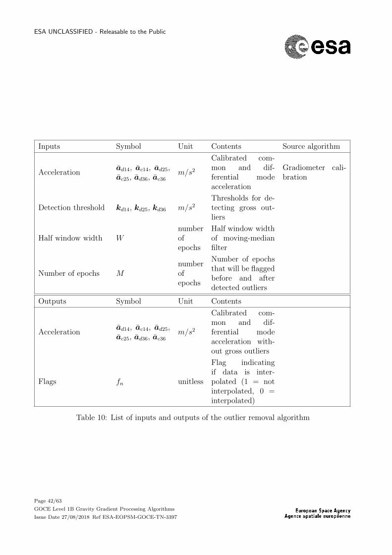
Accelerationad14, ac14, ad25,ac25, ad36, ac36
m/s2
Calibrated com-mon and dif-ferential modeacceleration
Gradiometer cali-bration
Detection threshold kd14, kd25, kd36 m/s2
Thresholds for de-tecting gross out-liers
Half window width Wnumberofepochs
Half window widthof moving-medianfilter
Number of epochs Mnumberofepochs
Number of epochsthat will be flaggedbefore and afterdetected outliers
Outputs Symbol Unit Contents
Accelerationad14, ac14, ad25,ac25, ad36, ac36
m/s2
Calibrated com-mon and dif-ferential modeacceleration with-out gross outliers
Flags fn unitless
Flag indicatingif data is inter-polated (1 = notinterpolated, 0 =interpolated)
Table 10: List of inputs and outputs of the outlier removal algorithm
Page 42/63
GOCE Level 1B Gravity Gradient Processing Algorithms
Issue Date 27/08/2018 Ref ESA-EOPSM-GOCE-TN-3397

ESA UNCLASSIFIED - Releasable to the Public
7 Angular rate and acceleration reconstruction
The star trackers provide the inertial attitude, from which we can determine the angular ratesof the satellite by differentiation of the attitude quaternions. The differentiation tilts the startracker noise PSD such that high-frequency is amplified and low-frequency noise is dampened.The star tracker angular rates are therefore accurate at low frequencies and less accurate athigh frequencies. We can determine the angular rates also by integrating the gradiometerangular rates (except for the integration constant), where the integration tilts the gradiometernoise PSD such that low-frequency noise is amplified and high-frequency noise is dampened.Thus, the gradiometer angular rates are accurate at high frequencies and less accurate at lowfrequencies. Obviously, the star tracker and gradiometer angular rates are synergetic and theangular rate and acceleration reconstruction takes advantage of this fact. In a nutshell, weapply a lowpass filter to the star tracker angular rates and a complementary highpass filter tothe gradiometer angular rates, and add results to arrive at the reconstructed angular rates. Thereconstructed angular accelerations are obtained by differentiating the reconstructed angularrates.
In the following, we provide details on the calculation of the star tracker and gradiometerangular rates as well as the angular rate and acceleration reconstruction algorithm. We willkeep the naming of the variables generic because the algorithm is used twice in the processing,one time prior to the gradiometer calibration to obtain a proxy for the angular accelerationsof the satellite and another time after the calibration of the gradiometer and correction ofmisalignments between star trackers and gradiometer.
7.1 Calculation of star tracker angular rates
The calculation of angular rates from the combined star tracker quaternions is straight forwardusing Eqs. (34) and (35). Due to the sign ambiguity of quaternions, we need to run Algorithm 4prior to the differentiation of quaternions. For the epochs when none of the star sensors isproviding a valid attitude, we interpolate the quaternions in order to be able to calculate theangular rates in all cases. This is needed because the filtering applied in the angular ratereconstruction is not designed to handle data gaps. Even a single missing attitude quaternionwould lead to a data gap of the length of the reconstruction filters, which is avoided by theinterpolation. We use cubic spline interpolation as specified in Section 2.2. The calculation ofangular rates is detailed in Algorithm 11.
Page 43/63
GOCE Level 1B Gravity Gradient Processing Algorithms
Issue Date 27/08/2018 Ref ESA-EOPSM-GOCE-TN-3397

ESA UNCLASSIFIED - Releasable to the Public
Inputs Symbol Unit Contents Source algorithm
Attitudequaternions
q unitlessOrientation of either CRFor GRF wrt. IRF
Either star tracker combi-nation or star tracker mis-alignment adjustment
Epochs tGPSsecond
Epochs of q Star tracker combination
Flags fq unitlessFlags for star tracker quater-nions (1 = valid, 0 = invalid)
Star tracker combination
Time step ∆t seconds
Time step for approximat-ing the first time derivative(shall be much smaller thansampling rate)
Control parameter
Outputs Symbol Unit Contents
Angularrates
ω rad/sAngular rates from com-bined star tracker quater-nions
Flags fω unitlessFlags for angular rates (1 =valid, 0 = invalid)
Table 11: List of inputs and outputs of algorithm for calculation of star tracker angular rates
7.2 Calculation of gradiometer angular rates
The angular rates from the gradiometer are calculated by numerical integration of the gradiome-ter angular accelerations as described in Algorithm 1. These processing steps are summarisedin Algorithm 12.
7.3 Calculation of filters for angular rate reconstruction
We use the same approach for calculating the angular rate reconstruction filters as Stummeret al. [2011], with the difference that we define the noise PSDs for star tracker and gradiometerangular rates differently. Here, we choose a simpler model that allows us to choose very easilythe frequency where the PSDs cross. It is defined by
PS = fαS and PG = cfαG (73)
where f is the frequency vector, PS and PG are the PSD of the star tracker and gradiometerangular rates, respectively, αS and αG are the slope of these PSDs in the logarithmic domain,and
c = (f cross)αS−αG (74)
Page 44/63
GOCE Level 1B Gravity Gradient Processing Algorithms
Issue Date 27/08/2018 Ref ESA-EOPSM-GOCE-TN-3397

ESA UNCLASSIFIED - Releasable to the Public
Algorithm 11 Calculation of star tracker angular rates
1: Run Algorithm 4 on the star tracker quaternions q to make them continuous2: Interpolate all quaternions for which fq,n = 0 using cubic spline interpolation as specified
in Section 2.2. Flags of interpolated quaternions remain fq,n = 0.3: for n← 1, N do . Normalize all quaternions (including interpolated ones)4: qn = qn/
√qTn qn
5: end for6: q = differentiate(t, q,∆t) . Algorithm 27: W1 = q∗1 q1 . Quaternion multiplication
8: ω1 = 2[W1,2 W1,3 W1,4
]T9: fω,1 = fq,1fq,2 . Multiply flags10: for n← 2, N − 1 do11: Wn = q∗n qn . Quaternion multiplication
12: ωn = 2[Wn,2 Wn,3 Wn,4
]T13: fω,n = fq,n−1fq,nfq,n+1 . Multiply flags14: end for15: WN = q∗N qN . Quaternion multiplication
16: ωN = 2[WN,2 WN,3 WN,4
]T17: fω,N = fq,N−1fq,N . Multiply flags
Algorithm 12 Calculation of gradiometer angular rates
1: ωx = −ad36y/Lz + ad25z/Ly2: ωy = −ad14z/Lx + ad36x/Lz3: ωz = −ad25x/Ly + ad14y/Lx4: ωx = integrate(t, ωx, K) . Algorithm 15: ωy = integrate(t, ωy, K)6: ωz = integrate(t, ωz, K)
is a scale factor depending on the frequency f cross that defines where PS and PG cross eachother. The length of the frequency vector is equal to the length of the filters, which we denoteby NF and must be an odd integer that is large enough to achieve sufficient resolution in thespectral domain. We recommend to use
NF ≈10
f cross. (75)
Since the components x, y and z of the angular rates are reconstructed independently, weomit the subscripts x, y and z in the following for simplicity. In practice, we have to run thealgorithms for the calculation of the angular rate reconstruction filters as well as the angularrate reconstruction itself three times, i.e. once per component. It is possible to use differentinput parameters such as f cross for each component.
Page 45/63
GOCE Level 1B Gravity Gradient Processing Algorithms
Issue Date 27/08/2018 Ref ESA-EOPSM-GOCE-TN-3397

ESA UNCLASSIFIED - Releasable to the Public
Inputs Symbol Unit Contents Source algorithm
Accelerations adij m/s2 Calibrated accelerationsEither satellite shakingor science mode gra-diometer calibration
Epochs tGPSsecond
Gradiometer measure-ment epochs
EGG NOM 1B files
Gradiometerarm length
Lx, Ly, Lz meters Gradiometer arm length
Factor K unitlessFactor defining the in-crease of epochs of theupsampled time series
Control parameter
Outputs Symbol Unit Contents
Angular rates ω rad/sAngular rates from gra-diometer
Table 12: List of inputs and outputs of algorithm for calculation of gradiometer angular rates
Inputs Symbol Unit Contents
Crossing frequency f cross Hz Frequency of equal spectral weights
Length of filter NF unitless Length of filter (odd integer)
Exponent αS, αG unitless Slopes of PSDs in logarithmic domain
Outputs Symbol Unit Contents
Filter coefficients FS, FG unitlessFilter coefficients for one component(x, y or z) of the angular rates
Table 13: List of inputs and outputs for calculation of angular rate reconstruction filters
7.4 Application of filters for angular rate reconstruction
The angular rate reconstruction filters calculated according to Algorithm 13 are symmetricmoving-average filters. Applying the filters is therefore a convolution in the time domain,which can be efficiently performed as an element-wise multiplication in the frequency domain.We use the symbol for notating elementwise multiplication, i.e.
a1
a2
...
aN
b1
b2
...
bN
=
a1b1
a2b2
...
aNbN
. (76)
Page 46/63
GOCE Level 1B Gravity Gradient Processing Algorithms
Issue Date 27/08/2018 Ref ESA-EOPSM-GOCE-TN-3397

ESA UNCLASSIFIED - Releasable to the Public
Algorithm 13 Calculation of filters for angular rate reconstruction
1: K = ceil(NF/2) . Index of mid frequency
2: f = 1NF
[0 1 · · · NF − 1
]T. Frequency vector
3: c = (f cross)αS−αG
4: PG = cfαG . Define PSDs5: PS = fαS
6: for n← 2, K do . Make PSD symmetric around mid frequency7: PS,NF−n+2 = PS,n8: PG,NF−n+2 = PG,n9: end for
10: WS = zeros(size(PS)) . Spectral weights for star tracker angular rates11: if αS − αG < 0 then . Spectral weight for zero frequency12: WS,1 = 013: else if αS − αG > 0 then14: WS,1 = 115: else16: WS,1 = c/(c+ 1)17: end if18: for n← 2, NF do19: WS,n = PG,n/(PG,n + PS,n) . Spectral weight for non-zero frequencies20: end for21: FS = ifft(WS) . Filter coefficients
22: FS =[FS,K+1 FS,K+2 · · · FS,NF
FS,1 FS,2 · · · FS,K
]. Resort coefficients
23: FG = −FS . Complementary filter24: FG,K = FG,K + 1
Generally, symmetric moving-average filters produce transient effects at the beginning and theend of the angular rate time series. Instead of cropping the filtered time series by half the filterlength, we use a different approach for reducing the transient effects. Since the length NF of thefilters is an input parameter to Algorithm 13, it is straight forward to generate shorter filters.For the first epoch of the filtered time series, we create a filter of length NF = 1 and apply itto the first value of the input time series; for the second epoch of the filtered time series, wecreate a filter of length NF = 3 and apply it to the first three values of the input time series;and so forth until we have reached half the length of the filter. We repeat the same procedurefor the end of the filtered time series. This approach avoids transient effects except for thefirst and last few epochs of the filtered time series, for which we extrapolate the gradiometerangular rates after fitting them to the sum of the filtered star tracker and gradiometer angularrates. The entire approach is detailed in Algorithm 14.
Page 47/63
GOCE Level 1B Gravity Gradient Processing Algorithms
Issue Date 27/08/2018 Ref ESA-EOPSM-GOCE-TN-3397

ESA UNCLASSIFIED - Releasable to the Public
Inputs Symbol Unit Contents
Crossing frequency f cross Hz Frequency of equal spectral weights
Length of filter NF unitless Length of filter (odd integer)
Exponent αS, αG unitless Slopes of PSDs in logarithmic domain
Number of epochs M unitless Number of epochs at beginning/end
Angular rates ωS, ωG rad/sOne component (x, y or z) of the startrackers and gradiometer angular rates
Outputs Symbol Unit Contents
Angular rates ω rad/sOne component (x, y or z) of the recon-structed angular rates
Angular accelerations ω rad/s2
One component (x, y or z) of the re-constructed angular accelerations (op-tional)
Table 14: List of inputs and outputs of angular rate reconstruction algorithm
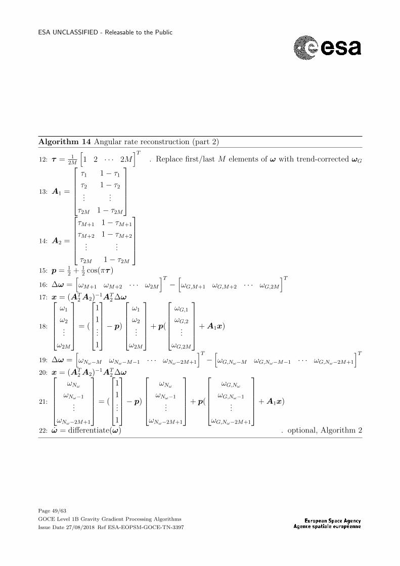
Algorithm 14 Angular rate reconstruction (part 1)
1: K = floor(NF/2)2: Create FG and FS of length NF using Algorithm 133: Nω = length(ωG) . Same length as ωS4: NFFT = 2ceil(log2(NF +Nω−1)) . Convolution of filters and angular rates5: h = ifft(fft(FG, NFFT ) fft(ωG, NFFT ) + fft(FS, NFFT ) fft(ωS, NFFT ))
6: ω =[hK+1 hK+2 · · · hK+Nω
]T7: for n← 1,min(K, ceil(Nω/2)) do . Apply shorter filters at beginning and end8: Create FG and FS of length 2n− 1 using Algorithm 13
9: ωn = F TG
ωG,1
ωG,2...
ωG,2n−1
+ F TS
ωS,1
ωS,2...
ωS,2n−1
10: ωNω−n+1 = F TG
ωG,Nω−2n+2
ωG,Nω−2n+3
...
ωG,Nω
+ F TS
ωS,Nω−2n+2
ωS,Nω−2n+3
...
ωS,Nω
11: end for
Page 48/63
GOCE Level 1B Gravity Gradient Processing Algorithms
Issue Date 27/08/2018 Ref ESA-EOPSM-GOCE-TN-3397
ESA UNCLASSIFIED - Releasable to the Public
Algorithm 14 Angular rate reconstruction (part 2)
12: τ = 12M
[1 2 · · · 2M
]T. Replace first/last M elements of ω with trend-corrected ωG
13: A1 =
τ1 1− τ1
τ2 1− τ2
......
τ2M 1− τ2M
14: A2 =
τM+1 1− τM+1
τM+2 1− τM+2
......
τ2M 1− τ2M
15: p = 1
2+ 1
2cos(πτ )
16: ∆ω =[ωM+1 ωM+2 · · · ω2M
]T−[ωG,M+1 ωG,M+2 · · · ωG,2M
]T17: x = (AT
2A2)−1AT2 ∆ω
18:
ω1
ω2
...
ω2M
= (
1
1...
1
− p)
ω1
ω2
...
ω2M
+ p(
ωG,1
ωG,2...
ωG,2M
+A1x)
19: ∆ω =[ωNω−M ωNω−M−1 · · · ωNω−2M+1
]T−[ωG,Nω−M ωG,Nω−M−1 · · · ωG,Nω−2M+1
]T20: x = (AT
2A2)−1AT2 ∆ω
21:
ωNω
ωNω−1
...
ωNω−2M+1
= (
1
1...
1
− p)
ωNω
ωNω−1
...
ωNω−2M+1
+ p(
ωG,Nω
ωG,Nω−1
...
ωG,Nω−2M+1
+A1x)
22: ω = differentiate(ω) . optional, Algorithm 2
Page 49/63
GOCE Level 1B Gravity Gradient Processing Algorithms
Issue Date 27/08/2018 Ref ESA-EOPSM-GOCE-TN-3397

ESA UNCLASSIFIED - Releasable to the Public
Page 50/63
GOCE Level 1B Gravity Gradient Processing Algorithms
Issue Date 27/08/2018 Ref ESA-EOPSM-GOCE-TN-3397
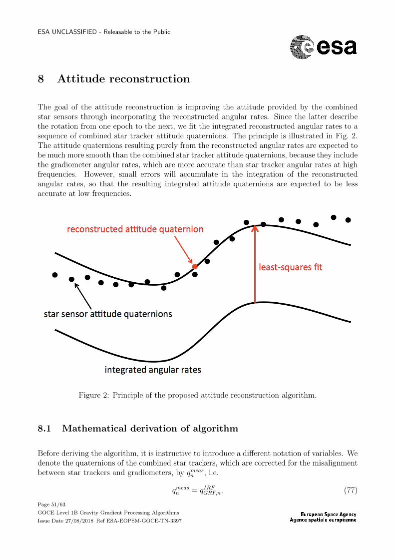
ESA UNCLASSIFIED - Releasable to the Public
8 Attitude reconstruction
The goal of the attitude reconstruction is improving the attitude provided by the combinedstar sensors through incorporating the reconstructed angular rates. Since the latter describethe rotation from one epoch to the next, we fit the integrated reconstructed angular rates to asequence of combined star tracker attitude quaternions. The principle is illustrated in Fig. 2.The attitude quaternions resulting purely from the reconstructed angular rates are expected tobe much more smooth than the combined star tracker attitude quaternions, because they includethe gradiometer angular rates, which are more accurate than star tracker angular rates at highfrequencies. However, small errors will accumulate in the integration of the reconstructedangular rates, so that the resulting integrated attitude quaternions are expected to be lessaccurate at low frequencies.
Figure 2: Principle of the proposed attitude reconstruction algorithm.
8.1 Mathematical derivation of algorithm
Before deriving the algorithm, it is instructive to introduce a different notation of variables. Wedenote the quaternions of the combined star trackers, which are corrected for the misalignmentbetween star trackers and gradiometers, by qmeasn , i.e.
qmeasn = qIRFGRF,n. (77)
Page 51/63
GOCE Level 1B Gravity Gradient Processing Algorithms
Issue Date 27/08/2018 Ref ESA-EOPSM-GOCE-TN-3397

ESA UNCLASSIFIED - Releasable to the Public
Further, we define the quaternion qtruen as the true (free of errors and noise) counterpart ofqmeasn and the rotation quaternion qrotn→n+k, which describes the rotation of the gradiometer fromepoch tn to tn+k in the sense of
qrotn→n+k = (qIRFGRF,n)∗qIRFGRF,n+k, (78)
where it is emphasised that qrotn→n+k is calculated by integrating the reconstructed angular rates,which we denote by ωn. With this notation, we can express the measured quaternion qmeasn+k asa rotated version of the true quaternion qmeasn , i.e.
qmeasn+k = qnoisen+k qtruen qrotn→n+k (79)
where qnoisen+k reflects the combined effect of the noise of the combined attitude quaternion qmeasn+k
and the noise of the rotation quaternion qrotn→n+k that results from the integration of the recon-structed angular rates. The noise quaternion qnoisen+k is assumed to represent a small rotation,i.e.
qnoisen+k =
1
εx,n+k/2
εy,n+k/2
εz,n+k/2
(80)
where εx,n+k, εy,n+k and εz,n+k are small angles as described in Section 3.
In order to explain the relation between the rotation quaternion qrotn→n+k and the reconstructedangular rates ωn, we decompose qrotn→n+k into a series of rotations,
qrotn→n+k = qrotn→n+1qrotn+1→n+2 . . . q
rotn+k−1→n+k, (81)
noting that the sequence of rotation is important as quaternions are not commutative. Eachquaternion qrotn+i→n+i+1 where i ∈ 0, . . . , k − 1 is calculated from the reconstructed angularrates according to
qrotn+i→n+i+1 =
[cos(φ/2)
sin(φ/2)e
](82)
where
φ =|ωn+i+1 + ωn+i|
2(83)
is the angle of rotation and
e =ωn+i+1 + ωn+i
|ωn+i+1 + ωn+i|(84)
is the rotation axis.
The measured quaternion qmeasn+k in Eq. (79) composes of the product of the noise quaternionqnoisen+k and the true quaternion qtruen , which are both unknown. Since this would lead us tothe least-squares adjustment according to the non-linear mixed model (Gauß-Helmert model),
Page 52/63
GOCE Level 1B Gravity Gradient Processing Algorithms
Issue Date 27/08/2018 Ref ESA-EOPSM-GOCE-TN-3397

ESA UNCLASSIFIED - Releasable to the Public
we reformulate Eq. (79) in the following such that we can use linear generalised least squares(Gauß-Markov model), which is much simpler to solve. We start with rearranging Eq. (79) to
qmeasn+k (qtruen qrotn→n+k)∗ = qnoisen+k . (85)
Now we define the relative error of the quaternions of epochs n and n+ k as
qreln,n+k = qnoisen (qnoisen+k )∗, (86)
which we can calculate according to Eq. (85) as
qreln,n+k = qmeasn (qtruen qrotn→n)∗(qmeasn+k (qtruen qrotn→n+k)∗)∗
= qmeasn (qtruen )∗qtruen qrotn→n+k(qmeasn+k )∗
= qmeasn qrotn→n+k(qmeasn+k )∗ (87)
noting that qrotn→n is a unit quaternion, i.e.
qrotn→n =
1
0
0
0
. (88)
It is important to realise that we can calculate the relative error of the quaternions qreln,n+k
from Eq. (87), even though it is the product of two unknown noise quaternions as described inEq. (86). Because of the latter, we assume that it represents a small rotation denoted by
qreln,n+k =
1
δx,n,n+k/2
δy,n,n+k/2
δz,n,n+k/2
. (89)
By rearranging Eq. (86) to
qreln,n+kqnoisen+k = qnoisen (90)
we can express the noise of epoch n+ k as the noise of epoch n multiplied by the relative error,or equivalently
dn,n+k + en+k = en +O(e2) (91)
where
dn,n+k =
δx,n,n+k
δy,n,n+k
δz,n,n+k
, en =
εx,nεy,n
εz,n
and en+k =
εx,n+k
εy,n+k
εz,n+k
. (92)
Page 53/63
GOCE Level 1B Gravity Gradient Processing Algorithms
Issue Date 27/08/2018 Ref ESA-EOPSM-GOCE-TN-3397
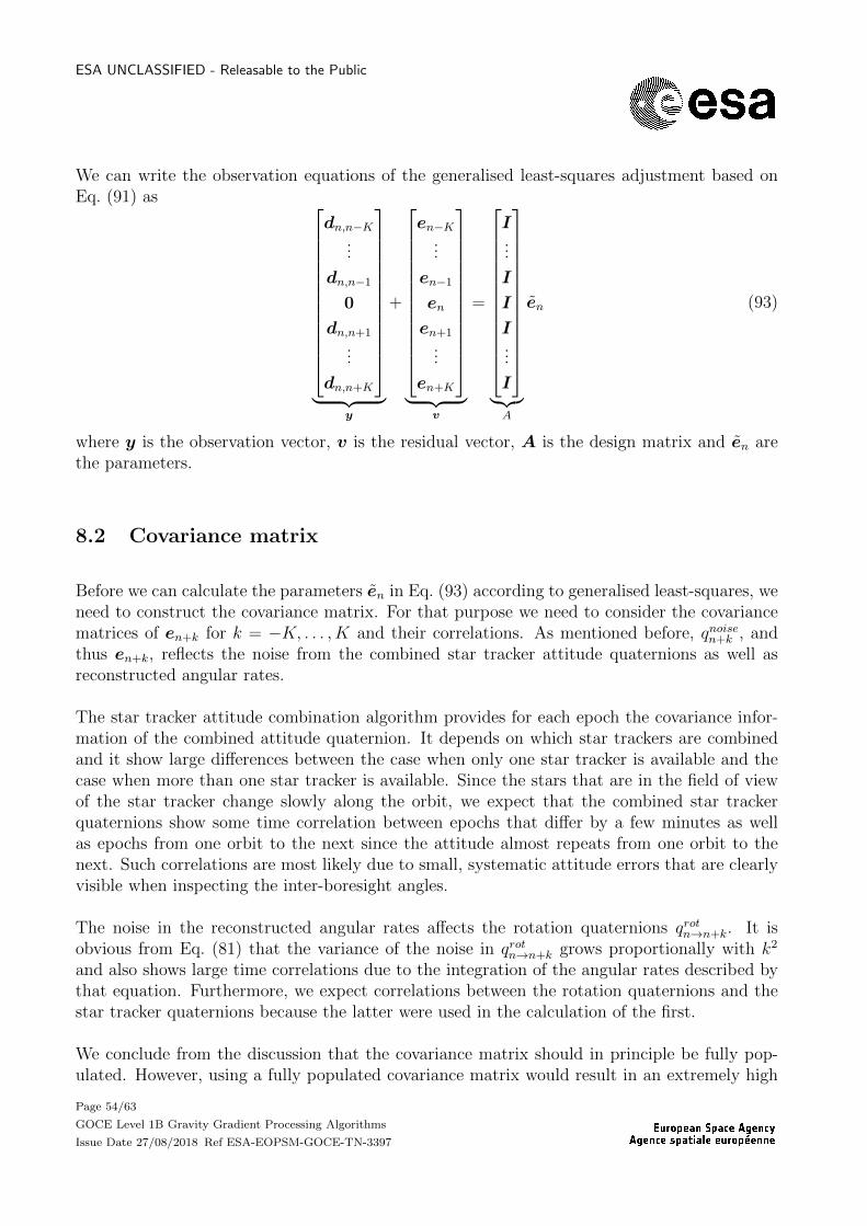
ESA UNCLASSIFIED - Releasable to the Public
We can write the observation equations of the generalised least-squares adjustment based onEq. (91) as
dn,n−K...
dn,n−1
0
dn,n+1
...
dn,n+K
︸ ︷︷ ︸
y
+
en−K...
en−1
en
en+1
...
en+K
︸ ︷︷ ︸
v
=
I...
I
I
I...
I
︸︷︷︸A
en (93)
where y is the observation vector, v is the residual vector, A is the design matrix and en arethe parameters.
8.2 Covariance matrix
Before we can calculate the parameters en in Eq. (93) according to generalised least-squares, weneed to construct the covariance matrix. For that purpose we need to consider the covariancematrices of en+k for k = −K, . . . ,K and their correlations. As mentioned before, qnoisen+k , andthus en+k, reflects the noise from the combined star tracker attitude quaternions as well asreconstructed angular rates.
The star tracker attitude combination algorithm provides for each epoch the covariance infor-mation of the combined attitude quaternion. It depends on which star trackers are combinedand it show large differences between the case when only one star tracker is available and thecase when more than one star tracker is available. Since the stars that are in the field of viewof the star tracker change slowly along the orbit, we expect that the combined star trackerquaternions show some time correlation between epochs that differ by a few minutes as wellas epochs from one orbit to the next since the attitude almost repeats from one orbit to thenext. Such correlations are most likely due to small, systematic attitude errors that are clearlyvisible when inspecting the inter-boresight angles.
The noise in the reconstructed angular rates affects the rotation quaternions qrotn→n+k. It isobvious from Eq. (81) that the variance of the noise in qrotn→n+k grows proportionally with k2
and also shows large time correlations due to the integration of the angular rates described bythat equation. Furthermore, we expect correlations between the rotation quaternions and thestar tracker quaternions because the latter were used in the calculation of the first.
We conclude from the discussion that the covariance matrix should in principle be fully pop-ulated. However, using a fully populated covariance matrix would result in an extremely high
Page 54/63
GOCE Level 1B Gravity Gradient Processing Algorithms
Issue Date 27/08/2018 Ref ESA-EOPSM-GOCE-TN-3397

ESA UNCLASSIFIED - Releasable to the Public
computational effort since one would have to invert a large matrix for each epoch. There-fore, we ignore time correlations and reduce thereby the covariance matrix to a block-diagonalstructure, with one 3 × 3 block per epoch. The computational effort will still be high, butmanageable for a single CPU. There are two properties that we take into account when con-structing the covariance matrix. The first is the covariance information that we get from thestar tracker combination and the second is the linearly increasing standard deviation of thenoise in the rotation quaternions. The ”slope” of the increase can be determined empiricallyfrom residuals between combined star tracker attitude quaternions, which are corrected for themisalignment between star trackers and quaternions, and the rotation quaternions resultingfrom the integration of the reconstructed angular rates.
The covariance matrix that we utilise has therefore a block-diagonal structure,
Σ =
Σn−K 0 · · · 0
0 Σn−K+1. . .
......
. . . . . . 0
0 · · · 0 Σn−K
, (94)
where each block of dimension 3× 3 is the sum
Σn+k = Σmeasn+k + Σrot
n+k (95)
of the covariance matrix Σmeasn+k of the combined star sensor quaternion and the covariance
matrix Σrotn+k of the rotation quaternion.
The covariance matrices Σmeasn+k of the combined star sensor quaternion are an output of Al-
gorithm 6, which provides the cofactor matrices Q1, . . .Q123 and the square-sum of residualsΩ. The latter still needs to be divided by the redundancy of the least-squares adjustment, inwhich the combined star tracker quaternions were estimated, in order to obtain the a posteriorivariance factor σ2
0. The redundancy R can be calculated from the flags fS1 , fS2 and fS3 of theresampled and star tracker quaternions and the flags f of the combined star trackers by
R = 3N∑n=1
(fn − fS1,n − fS2,n − fS3,n), (96)
which gives then an a posteriori variance factor
σ20 =
Ω
R. (97)
The covariance matrices for the different combinations of available star trackers are the productof the variance factor and the cofactor matrices, i.e.
ΣmeasS1,n+k = σ2
0Q1, ΣmeasS2,n+k = σ2
0Q2, etc. (98)
Page 55/63
GOCE Level 1B Gravity Gradient Processing Algorithms
Issue Date 27/08/2018 Ref ESA-EOPSM-GOCE-TN-3397

ESA UNCLASSIFIED - Releasable to the Public
Since the cofactor matrices are constant, we list their values in Eqs. (99–105). The a posteriorivariance factor σ2
0 is approximately σ20 = 132 µrad2.
Q1 =
1.000121521459708 0.095222836108324 −0.054435478192699
0.095222836108324 75.615532876845165 −42.655022458413313
−0.054435478192699 −42.655022458413320 25.384345601751161
(99)
Q2 =
1.001561466393628 −0.131503870039127 0.370525932944455
−0.131503870039127 12.075017626225865 −31.205022613483280
0.370525932944455 −31.205022613483280 88.923420907434434
(100)
Q3 =
41.413359274606734 42.610626719061884 −23.495051626509660
42.610626719061884 45.927359219359751 −24.772473572404802
−23.495051626509660 −24.772473572404802 14.659281505935640
(101)
Q12 =
0.500011447421263 −0.002903273148382 0.004247636496021
−0.002903273148382 1.919411345174103 −1.616662280334516
0.004247636496021 −1.616662280334516 2.502024213487087
(102)
Q13 =
0.965936848197282 0.968247299647752 −0.543564953526007
0.968247299647752 2.879509027619699 −1.339618855085098
−0.543564953526007 −1.339618855085097 1.254213201185986
(103)
Q23 =
0.790153006185965 0.391922949490108 −0.408574304412965
0.391922949490108 1.085989398656493 −0.709773601283014
−0.408574304412965 −0.709773601283014 1.515784721963927
(104)
Q123 =
0.436398899448459 0.214237386367438 −0.179540976548104
0.214237386367438 0.986366903459979 −0.587553396581192
−0.179540976548104 −0.587553396581192 0.931510054952443
(105)
The covariance matrix of the rotation quaternion Σrotn+k is modelled as the diagonal matrix
Σrotn+k =
σ2x 0 0
0 σ2y 0
0 0 σ2z
(106)
Page 56/63
GOCE Level 1B Gravity Gradient Processing Algorithms
Issue Date 27/08/2018 Ref ESA-EOPSM-GOCE-TN-3397
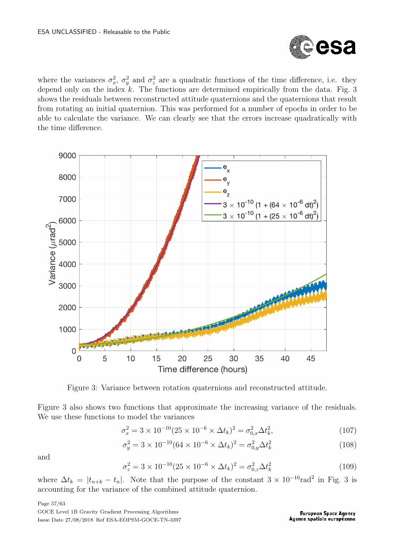
ESA UNCLASSIFIED - Releasable to the Public
where the variances σ2x, σ
2y and σ2
z are a quadratic functions of the time difference, i.e. theydepend only on the index k. The functions are determined empirically from the data. Fig. 3shows the residuals between reconstructed attitude quaternions and the quaternions that resultfrom rotating an initial quaternion. This was performed for a number of epochs in order to beable to calculate the variance. We can clearly see that the errors increase quadratically withthe time difference.
Figure 3: Variance between rotation quaternions and reconstructed attitude.
Figure 3 also shows two functions that approximate the increasing variance of the residuals.We use these functions to model the variances
σ2x = 3× 10⁻¹⁰(25× 10−6 ×∆tk)
2 = σ20,x∆t
2k, (107)
σ2y = 3× 10⁻¹⁰(64× 10−6 ×∆tk)
2 = σ20,y∆t
2k (108)
andσ2z = 3× 10⁻¹⁰(25× 10−6 ×∆tk)
2 = σ20,z∆t
2k (109)
where ∆tk = |tn+k − tn|. Note that the purpose of the constant 3 × 10⁻¹⁰rad2 in Fig. 3 isaccounting for the variance of the combined attitude quaternion.
Page 57/63
GOCE Level 1B Gravity Gradient Processing Algorithms
Issue Date 27/08/2018 Ref ESA-EOPSM-GOCE-TN-3397

ESA UNCLASSIFIED - Releasable to the Public
8.3 Algorithm
The attitude reconstruction is detailed in Algorithm 15. It should be noted that in case somecombined star tracker quaternions are not available (flag is zero), they will simply not beused in the attitude reconstruction, with the only exception of the centre epoch for which wereconstruct the attitude quaternion. Technically, they receive zero weight in the least squaresestimation by setting
Σ−1n+k = (Σmeas
n+k + Σrotn+k)
−1 = 0. (110)
Inputs Symbol Unit Contents Source algorithm
Attitude quaternions qmeas unitlessOrientation ofGRF wrt. IRF
Star tracker combi-nation
Angular rates ω rad/sRotation rate ofGRF wrt. IRF
Angular rate re-construction
Flag for star trackers fS1 , fS2 , fS3 unitless1 = valid, 0 = in-valid
Star tracker combi-nation
Covariance matricesΣS1 , ΣS2 , ΣS3 ,ΣS12 , ΣS13 ,ΣS23 , ΣS123
rad2
Covariance matrixof combined startracker attitude
Star tracker combi-nation
Variances σ20,x, σ
20,y, σ
20,z rad2
Variance functionfor reconstructedangular rates
Data analysis (cf.Fig. 3
Half window width K unitlessNumbers of epochsto the left/right ofthe centre epoch
Outputs Symbol Unit Contents
Attitude quaternions qrec unitlessOrientation ofGRF wrt. IRF
Rotation matrices Rrec unitlessOrientation ofGRF wrt. IRF
Table 15: List of inputs and outputs of attitude reconstruction algorithm
Page 58/63
GOCE Level 1B Gravity Gradient Processing Algorithms
Issue Date 27/08/2018 Ref ESA-EOPSM-GOCE-TN-3397

ESA UNCLASSIFIED - Releasable to the Public
Algorithm 15 Attitude reconstruction algorithm (part 1)
1: Run Algorithm 4 on qmeas
2: Interpolate quaternions qmeasn where fS1,n = fS2,n = fS3,n = 0 using cubic spline interpola-tion described in Section 2.2. Flags of interpolated quaternions remain zero.
3: for n← 1, N do . Normalize quaternions (including interpolated ones)4: qmeasn = qmeasn /
√(qmeasn )T qmeasn
5: end for6: for n← 1, N − 1 do . Calculate rotation quaternions for later use7: ω ← ωn+1+ωn
2(tn+1 − tn)
8: qrotn→n+1 ←
[cos(|ω|/2)sin(|ω|/2)|ω| ω
]. The hat designates that quaternions are stored
9: end for10: for n← 1, N do . Reconstruct attitude (exclude first/last K epochs)11: if fS1,n = 0 and fS2,n = 0 and fS3,n = 0 then12: qrecn = qmeasn
13: f recn = 014: else15: Σmeas
n ← ΣS1 or ΣS2 or . . . ΣS123 . Depending on fS1,n, fS2,n and fS3,n
16: N ← (Σmeasn )−1 . Initialise normal equation matrix
17: b←[0 0 0
]T. Initialise right-hand side of normal equations
18: qrotn→n+k ←[1 0 0 0
]T. Initialise rotation quaternion (k = 0)
19: for k ← 1,min(K,N − n) do20: qrotn→n+k ← qrotn→n+kq
rotn+k−1→n+k
21: if fS1,n+k = 1 or fS2,n+k = 1 or fS3,n+k = 1 then22: qreln,n+k ← qmeasn qrotn→n+k(q
measn+k )∗
23: dn,n+k ← 2[qreln,n+k(2) qreln,n+k(3) qreln,n+k(4)
]T24: Σmeas
n+k ← ΣS1 or . . . ΣS123 . Depending on fS1,n+k, fS2,n+k and fS3,n+k
25: Σrotn+k ←
σ2x,0 0 0
0 σ2y,0 0
0 0 σ2z,0
(tn − tn+k)2
26: Σn+k ← Σmeasn+k + Σrot
n+k
27: N ←N + Σ−1n+k
28: b← b+ Σ−1n+kdn,n+k
29: end if30: end for
Page 59/63
GOCE Level 1B Gravity Gradient Processing Algorithms
Issue Date 27/08/2018 Ref ESA-EOPSM-GOCE-TN-3397

ESA UNCLASSIFIED - Releasable to the Public
Algorithm 15 Attitude reconstruction algorithm (part 2)
31: qrotn→n+k ←[1 0 0 0
]T. Initialise rotation quaternion (k = 0)
32: for k ← −1,max(−K, 1− n) do33: qrotn→n+k ← qrotn→n+k(q
rotn+k→n+k+1)∗ . This line is different to the previous for-loop
34: if fS1,n+k = 1 or fS2,n+k = 1 or fS3,n+k = 1 then35: qreln,n+k ← qmeasn qrotn→n+k(q
measn+k )∗
36: dn,n+k ← 2[qreln,n+k(2) qreln,n+k(3) qreln,n+k(4)
]T37: Σmeas
n+k ← ΣS1 or . . . ΣS123 . Depending on fS1,n+k, fS2,n+k and fS3,n+k
38: Σrotn+k ←
σ20,x 0 0
0 σ20,y 0
0 0 σ20,z
(tn − tn+k)2
39: Σn+k ← Σmeasn+k + Σrot
n+k
40: N ←N + Σ−1n+k
41: b← b+ Σ−1n+kdn,n+k
42: end if43: end for44: e = N−1b
45: qrecn ← 1√1+eT e/4
[1
−e/2
]qmeasn . Including normalisation of quaternion
46: f recn = 1
47: Rrecn =
[(qrecn,0)2 + (qrecn,1)2 − (qrecn,2)2 − (qrecn,3)2 2(qrecn,1q
recn,2 + qrecn,0q
recn,3) 2(qrecn,1q
recn,3 − qrecn,0q
recn,2)
2(qrecn,1qrecn,2 − qrecn,0q
recn,3) (qrecn,0)2 − (qrecn,1)2 + (qrecn,2)2 − (qrecn,3)2 2(qrecn,2q
recn,3 + qrecn,0q
recn,1)
2(qrecn,1qrecn,3 + qrecn,0q
recn,2) 2(qrecn,2q
recn,3 − qrecn,0q
recn,1) (qrecn,0)2 − (qrecn,1)2 − (qrecn,2)2 + (qrecn,3)2
]48: end if49: end for
Page 60/63
GOCE Level 1B Gravity Gradient Processing Algorithms
Issue Date 27/08/2018 Ref ESA-EOPSM-GOCE-TN-3397

ESA UNCLASSIFIED - Releasable to the Public
9 Gravity gradient calculation
The calculation of the gravity gradients is provided in Algorithm 16.
Inputs Symbol Unit Contents Source algorithm
Acceleration ad14, ad25, ad36 m/s2
Calibrated differ-ential mode accel-eration
Gradiometer cali-bration in sciencemode
Angular rates ω rad/sRotation rate ofGRF wrt. IRF
Angular rate re-construction
Arm length Lx, Ly, Lz mLengths of the gra-diometer arms
Outputs Symbol Unit Contents
Gravity gradientsVxx, Vyy, Vzz,Vxy, Vxz, Vyz
s−2 Gravity gradientsin GRF
Table 16: List of inputs and outputs of attitude reconstruction algorithm
Algorithm 16 Gravity gradient calculation algorithm
1: for n← 1, N do2: Vxx,n = −2ad14x,n/Lx − ω2
y,n − ω2z,n
3: Vyy,n = −2ad25y,n/Ly − ω2x,n − ω2
z,n
4: Vzz,n = −2ad36z,n/Lz − ω2x,n − ω2
y,n
5: Vxz,n = −ad14z,n/Lx − ad36x,n/Lz + ωx,nωz,n6: Vxy,n = −ad25x,n/Ly − ad14y,n/Lx + ωx,nωy,n7: Vyz,n = −ad36y,n/Lz − ad25z,n/Ly + ωy,nωz,n8: end for
Page 61/63
GOCE Level 1B Gravity Gradient Processing Algorithms
Issue Date 27/08/2018 Ref ESA-EOPSM-GOCE-TN-3397

ESA UNCLASSIFIED - Releasable to the Public
Page 62/63
GOCE Level 1B Gravity Gradient Processing Algorithms
Issue Date 27/08/2018 Ref ESA-EOPSM-GOCE-TN-3397
ESA UNCLASSIFIED - Releasable to the Public
References
P. Groves. Principles of GNSS, inertial, and multisensor integrated navigation systems. ArtechHouse, Boston/London, second edition, 2013.
L. Romans. Optimal combination of quaternions from multiple star cameras, 2003. URLftp://podaac.jpl.nasa.gov/allData/grace/docs/quaternion_memo.pdf. Last accessed31 May 2018.
C. Stummer, T. Fecher, and R. Pail. Alternative method for angular rate determinationwithin the GOCE gradiometer processing. J Geod, 85:585–596, 2011. doi: 10.1007/s00190-011-0461-3.
Page 63/63
GOCE Level 1B Gravity Gradient Processing Algorithms
Issue Date 27/08/2018 Ref ESA-EOPSM-GOCE-TN-3397


![A BAYESIAN APPROACH TO INVERT GOCE GRAVITY GRADIENTSearth.esa.int/goce04/goce_proceedings/54_pajot.pdf · · 2015-05-28A BAYESIAN APPROACH TO INVERT GOCE GRAVITY GRADIENTS ... [16].](https://static.fdocuments.net/doc/165x107/5abebc7b7f8b9ad8278d8e80/a-bayesian-approach-to-invert-goce-gravity-bayesian-approach-to-invert-goce-gravity.jpg)

