TECHNICAL --- NASA REPORT

T E C H N I C A L

R E P O R T N A S A T R R-368 ' - - -

- r e LOAN COPY: ~ ~ n ~ f i i r ; l zz fi

-= KIRTLAND AFB, IyI- E AFWL (DOGE)

NUMERICAL SOLUTION OF THE EQUATIONS FOR COMPRESSIBLE LAMINAR, TRANSITIONAL, AND TURBULENT BOUNDARY LAYERS AND '

COMPARISONS WITH EXPERIMENTAL DATA

by Julius E. Hurris

Lungley Reseurcb Center Hdmpton, vu. 23365

. .

N A T I O N A L AERONAUTICS A N D SPACE A D M I N I S T R A T I O N W A S H I N G T O N , Dr C. A U G U S T 1971

TECH LIBRARY KAFB, NM

19. Security Classif. (of this report)

Unclassified

I 111111 I1111 11111 Hill llllt lllll lllll lilt 1111

20. Security Claaif. (of this page) 21. NO. of pages 22. Price'

Unclassified 84 $3.00 _ _ . -~

-. . - - ~ ~

1. Report No. I 2. Government Accession No.

.- 4. Title and Subtitle

NUMERICAL SOLUTION O F THE EQUATIONS FOR COM- PRESSIBLE LAMINAR. TRANSITIONAL. AND TURBULENT BOUNDARY LAYERS AND COMPARISONS WITH EXPERI- MENTALDATA

9. Performing Organization Name and Address

NASA Langley Research Center Hampton, Va. 23365

- 12. Sponsoring Agency Name and Address

National Aeronautics and Space Administration Washington, D.C. 20546

_ ~ _ 15. Sumlementarv Notes

~

5. Report Date

6.- Performing Organization Code August 1971

8. Performing Organization Report No.

L-7660 10. Work Unit No.

136-13-01 11. Contract or Grant No.

._

13. Type of Report and Period Covered

Technical Report - .

14. Sponsoring Agency Code

. . The information presented herein is based in par t upon a thes i s entitled "Numerical

Solution of the Compressible Laminar , Transitional, and Turbulent Boundary Layer Equa- tions With Comparisons to Experimental Data" submitted in par t ia l fulfillment of the requirements for the degree of Doctor of Philosophy in Aerospace Engineering, Virginia Polytechnic Institute and State University, Blacksburg, Virginia, May 1970.

-.

16. Abstract

A numerical method for solving the equations for laminar , transitional, and turbulent compressible boundary layers for e i ther planar o r axisymmetr ic flows is presented. The fully developed turbulent region is treated by replacing the Reynolds stress terms with an eddy viscosity model. The mean propert ies of the transitional boundary layer are calculated by multiplying the eddy viscosity by an intermittency function based on the statistical production and growth of the turbulent spots. A specifiable turbulent Prandtl number relates the turbulent flux of heat t o the eddy viscosity. A three-point implicit finite-difference scheme is used t o solve the system of equations. The momentum and energy equations are solved simultaneously without iteration. Numerous test cases are compared with experimental data f o r supersonic and hypersonic flows; these cases include flows with both favorable and mildly unfavorable p re s su re gradient his tor ies , mass flux a t the wall, and t ransverse curvature.

- .- _. 17. Key Words (Suggested by Author(s)) .

Laminar , transitional, and turbulent boundary

Numerical solution Compressible boundary layers

layers

18. Distribution Statement

Unclassified - Unlimited

NUMERICAL SOLUTION OF THE EQUATIONS

FOR COMPRESSIBLE LAMINAR, TRANSITIONAL, AND

TURBULENT BOUNDARY LAYERS AND COMPARISONS

WITH EXPEFUMENTAL DATA*

By Julius E. Harr i s Langley Research Center

SUMMARY

A numerical method for solving the system of equations which govern the mean flow properties of laminar, transitional, and turbulent compressible boundary layers for either planar or axisymmetric flows is presented. The turbulent boundary layer is treated by a two-layer concept with appropriate eddy viscosity models used for each layer to replace the Reynolds s t r e s s term. A specifiable static turbulent Prandtl number relates the turbulent heat flux t e rm to the Reynolds s t ress . The mean properties in the transitional boundary layer a r e calculated by multiplying the eddy viscosity by an intermittency function based on the statistical production and growth of the turbulent spots. The numerical method used to solve the system of equations is a three-point implicit finite-difference scheme. The momentum and energy equations a r e solved simultaneously without iteration.

A number of test cases a r e compared with experimental data for supersonic and hypersonic flows over planar and axisymmetric geometries. These test cases include laminar. transitional, and turbulent boundary-layer flows with both favorable and unfavorable pressure-gradient histories. M a s s flux at the wall and transverse curvature effects a r e considered. The results show that the system of equations and the numerical technique provide accurate predictions for laminar, transitional, and turbulent compressible boundary-layer flows.

*The information presented herein is based in part upon a thesis entitled "Numeri- cal Solution of the Compressible Laminar, Transitional, and Turbulent Boundary Layer Equations With Comparisons to Experimental Data," submitted in partial fulfillment of the requirements for the degree of Doctor of Philosophy in Aerospace Engineering, Virginia Polytechnic Institute and State University, Blacksburg, Virginia, May 1970.

INTRODUCTION

The boundary-layer concept first introduced by Prandtl (ref. 1) in 1904 divides the flow field over an arbi t rary surface into two distinct regions; an inviscid outer region in which solutions to the Euler equations describe the flow-field characteristics, and a viscous inner region where the classical boundary-layer equations apply. The boundary- layer region may be further categorized as to type, namely, laminar, transitional, and turbulent.

The laminar boundary layer has received considerable attention over the past 60 years. Reviews of early methods a r e presented in references 2 to 4. A review of similar and local similarity solutions is presented in reference 5. In the early part of the past decade, the complete nonsimilar laminar equations were solved to a high degree of accuracy by finite-difference techniques. (See Blottner, ref. 6.)

The mean flow within the transition region has not been studied as extensively as either the location of transition or the characteristics of the fully developed turbulent boundary layer. There have been many experimental studies where the heat transfer at the wall was measured, but these studies reveal little of the flow structure away from the wall. A few experimental studies have been made in which the instantaneous behavior of the transitional boundary layer was reported for both incompressible (refs. 7 to 9) and compressible flows (ref. 10) but more detailed work is still required. The available transitional region data, although limited in extent, does allow workable models of the mean flow structure in the transition region to be formulated and applied tentatively to compressible flow systems. These crude models a re generally based on the transport models for fully developed turbulent flows modified by some intermittency distribution. Reviews of transition and the transitional region have recently been presented by Ssvulescu (ref. 11) and Morkovin (ref. 12). (See, also, ref. 13.)

Compressible turbulent boundary-layer flows have received accelerated study over the past decade. At first most of the work was experimental, the main objective being development of empirical o r semiempirical correlation techniques. Little effort was devoted to obtaining numerical solutions of the equations for turbulent boundary layers until a few years ago. The principal difficulties were associated with modeling the turbulent transport t e rms as well as developing techniques for obtaining solutions on existing digital computer systems. Even today, because of the limited understanding of these turbulent transport processes, completely general solutions of the mean turbulent boundary-layer equations a r e not possible. However, by modeling the turbulent transport t e rms through eddy viscosity o r mixing-length concepts, it is possible to solve the system of equations directly. Reviews of recent analytical advances a r e contained in

2

reference 14 for incompressible flow. (See ref. 15 for compilation of incompressible data.) Similar material for compressible flows is presented in references 16 and 17.

A number of papers have been presented over the past decade in which attempts have been made to connect the three boundary-layer flow regions (laminar, transitional, and turbulent) so that one system of equations could be used to describe compressible boundary-layer flows. Persh (ref. 18) appears to be one of the first t o develop reason- ably accurate solutions for the transitional region. Persh used an empirical correlation of velocity profile data together with the streamwise momentum equation to predict the characteristics of transitional flow; although limited 'in application, it did present a method with which the laminar and turbulent regions could be tied together. Weber (ref. 19) used mixing-length theory and an intermittency factor based on the probability equation of Emmons (ref. 20) to calculate velocity profiles which were in fair agreement with existing experimental data. (See also Masaki and Yakura (ref. 21).) Martellucci, Rie, and Sontowski (ref. 22) were among the first to define an effective viscosity model for laminar, transitional, and turbulent compressible boundary-layer flows. (See also, Harris (ref. 23), Adams (ref. 24), and Kuhn (ref. 25)). Fish and McDonald (ref. 26) have developed a solution technique in which the mixing length at each streamwise station is governed by an integral solution of the turbulent kinetic energy equation with the free- s t ream turbulence intensity used as a boundary condition. The most significant feature of the Fish-McDonald technique is that the transition location and the extent of the transitional flow a r e not required as inputs to the solution. applied only to incompressible boundary-layer flows. Donaldson (ref. 28)).

The method has currently been (See also, Glushko (ref. 27) and

The present paper presents a system of equations that a r e applicable to laminar, transitional, and turbulent compressible boundary layers and a numerical technique for obtaining accurate solutions of the system for either planar o r axisymmetric perfect gas flows. The numerical technique is similar to that first developed by FlGgge-Lotz and Blottner (ref. 29) and la ter improved by Davis and Flcgge-Lotz (ref. 30). The momentum and energy equations remain coupled and a re solved simultaneously in the transformed plane without iteration. (Difference relations and coefficients for the difference equations are developed in appendixes A and B, respectively.) The procedure,is very efficient fo r parabolic systems where only two governing equations a r e required; however, as the number of equations increases beyond two, the method becomes increasingly inefficient because of the digital computer storage requirements. (See ref. 6.) The numerical technique yields accurate results for compressible laminar, transitional, and turbulent boundary layers with pressure gradients, heat transfer, and mass transfer at the wall. The method treats the fully developed turbulent region by replacing the Reynolds s t r e s s t e r m s with an eddy viscosity model. A specifiable static turbulent Prandtl number function relates the turbulent f lux of heat to the eddy viscosity model. The mean

3

properties of the transitional boundary layer are calculated by multiplying the eddy viscosity by an intermittency function based on the statistical production and growth of the turbulent spots. The eddy viscosity model is based upon existing experimental data.

SYMBOLS

A damping function (eq. (38))

(l) B(l) C(l ) *n 9 n 9 n 9

Dn 3 n ,Fn 9 n

coefficients in difference equation (66) and defined by equations (B3) to (B9) tu &) (1) ($1)

A(2) B(2) c(2) coefficients in difference equation (67) and defined by equa- n 9 n 9 n ’

skin-friction coefficient, TW

defined in equations (B45) and (B46)

specific heat at constant pressure

length defined in figure 13(a)


defined in equation (B39)

velocity ratio, - U

ue b v )

(PU) e mass injection parameter, -




G

H

H1,H2,H3,. . .,Hl1,HI2

a typical quantity in boundary layer

a typical quantity in boundary layer (see appendix A)

coefficients defined by equations (B17) to (B28)

heat-transfer coefficient

index used in grid-point notation (eq. (64))

flow index; j = 0 planar flow, j = 1 axisymmetric flow

grid-point-spacing parameter (eq. (64))

constant in eddy viscosity model (eq. (36))

constant in eddy viscosity model (eq. (41))

thermal conductivity

eddy conductivity (eq. (9))

reference length


defined in equations (28)

mixing length (eq. (36))

Mach number

grid-point index (fig. 7)

number of grid points at each x-station (fig. 7)

Prandtl number,

static turbulent Prandtl number (eq. (10))

C P

I(I

5

NSt

n

P

P

Q

Re

Re ,x

Re ,i

Re ,Axt

Re,e

Rm ,d

r

'f

rn

1"O

S

T

6

h Stanton number, - CpPU

index defined in figure 7

coefficient in correlation equation (55)

pressure


heat-transfer rate


ue unit Reynolds number, - V e

ue x Reynolds number based on x, A V e

U e Reynolds number at transition, ve xt,i

Reynolds number based on transition extent, --(xt,f ue - x ~ , ~ )

transition Reynolds number based on displacement thickness, v, ue 6t *

Reynolds number based on momentum thickness, k) 19

u,d free-stream Reynolds number based on diameter, - V ,

radial coordinate (fig. 1)

recovery factor (eq. (75))

nose radius

body radius (fig. 1)

Sutherland visco'sity constant ( 1 9 8 . 6 O R (110.3O K))

static temperature


defined in equation (B4 1)

transverse curvature t e rm (eqs. (21))

velocity component in x-direction (fig. 1)

law-of -wall coordinate, - U

friction velocity, i q ur

transformed normal velocity component (eq. (24))


velocity component in y-direction

velocity component defined by equation (7)

9x2 9x3 9x4 9 x 5 functions of grid-point spacing defined by equations (A4) to (A8)

X boundary-layer coordinate tangent to surface

end of transition 5 ,f

xt ,i

Y1 ,Y2,Y3,Y4,Y5,Y6

y7 ,y8 pYg 9y10

Y

Y+ law of wall coordinate,

Ym defined in figure 4

Z body coordinate (fig. 1)

a! defined in equations (28)

beginning of transition

functions of grid-point spacing defined by equations (A12) to (A17)

functions defined by equations (70)

boundary-layer coordinate normal t o surface

P r

7

P

r

Y

- Y

Ax

&[,A17

6

6*

* Ginc

E

- E

A

€

17

0

8

x

P

V

defined in equations (28)

streamwise intermittency distribution (eq. (57))

ratio of specific heats

transverse intermittency distribution (eq. (44))

grid-point spacing in physical plane

transition extent, xt,f - xt,i

grid-point spacing in transformed plane (see fig. 7)

boundary-layer thickness

displacement thickness

incompressible displacement thickness

eddy viscosity

eddy viscosity function defined in equation (15)

defined in equation (74)

eddy viscosity function defined in equation (16)

transformed normal boundary -1aye r coordinate

static temperature ratio (eqs. (23))

momentum thickness


molecular viscosity

P kinematic viscosity, - P

8

- V

P

7

X

Subscripts :

e

i

m

max

min

n

0

sl

average kinematic viscosity

transformed streamwise boundary-layer coordinate


functions defined in equations (48) to (50)

density

shear s t r e s s

angle between local tangent to surface and center line of body (see fig. 1)

vorticity Reynolds number (eq. (54))

maximum local value of x (fig. 5)

value of xmax at transition (stability index)

functional relation (see eq. (62))

edge value o r based on edge conditions

inner region of turbulent layer

mesh point in [-direction (see fig. 7)

maximum value

minimum value

mesh point in q-direction (see fig. 7)

outer region of turbulent layer

sublayer edge

9

SP

t

U

W

00

stagnation point

total condition

uniform or average value

wall value

free s t ream

Superscripts:

j flow index

? fluctuating component

- t ime average value

Other notation:

TVC transverse cur vatu re

A coordinate used as a subscript means partial differential with respect to the coordinate. (See eq. (Al).)

EQUATIONS FOR THE LAMINAR, TRANSITIONAL, AND

TURBULENT COMPRESSIBLE BOUNDARY LAYER

This section presents the governing equations for the compressible boundary layer together with the required boundary conditions. The eddy viscosity and eddy conductivity models used to represent the apparent turbulent shear and heat-flux t e rms appearing in the mean turbulent boundary-layer equations are discussed.

Physical Plane

Geometry and notation.- The orthogonal coordinate system is presented in figure 1. The boundary-layer coordinate system is denoted by X and Y which a r e tangent to and normal to the surface, respectively. The origin of both the boundary-layer coordinate axes system X,Y and the body coordinate axes system Z,R is located at the stagnation point for blunt bodies as shown in figure 1 or at the leading edge for sharp-tipped bodies.

10

F i g u r e 1.- Coordinate system and no ta t ion .

The velocity components u and v are oriented in the X- and Y-direction, respectively. Transve'rse curvature t e rms a r e retained because of their importance in the development of boundary-layer flows over slender bodies of revolution where the boundary-layer thickness may become of the order of the body radius ro. The angle $I is the angle between the Z axis and local tangent evaluated at (x,O). The coordinates ( ~ , i , O ) and ( x ~ , ~ , O ) represent the location at which transition is initiated and completed, respectively..

is mathem-atically described by the continuity, Navier-Stokes, and energy equations together with an equation of state, a heat conductivity law, and a viscosity law. For flows at large Reynolds number, Prandtl (ref. 1) has shown that the Navier-Stokes and energy equations can be simplified to a form now recognized as the classical boundary-layer equations. These equations may be written as follows:

~~ Differential equations.- The flow of a compressible, viscous , heat conducting fluid

11

Continuity:

"(rjpu) ax + +(rjpv) = o

Momentum:

p u - + v - =--+---r p - (: :) k . 3 3 dp "[j(

Energy:

Osborne Reynolds (ref. 31) in 1883 was the first to observe and study the phenomena of transition from laminar to turbulent flow. Reynolds assumed that the instantaneous fluid velocity satisfied the Navier-Stokes equations and that the instantaneous velocity could be separated into mean and fluctuating components. The result of his early work was a set of Reynolds equations which differed from the Navier-Stokes equations only through the additional te rms called the Reynolds stresses. These equations can be reduced through the boundary-layer approximations and written in te rms of the mean variables as follows (ref. 32):

Continuity:

Momentum:

E ne rgy :

p [; U-(C P T ) + ( v +- y);( - CpT) ]

(4)

12

The reduction of the Reynolds equations to the mean turbulent boundary-layer form presented in equations (4), (5), and (6) requires a number of stringent assumptions based on an order-of-magnitude analysis. These assumptions together with the various correlation te rms which a r e neglected a r e discussed by Van Driest (ref. 32). However, for hypersonic flows where the boundary-layer thickness may increase rapidly and the density gradients are large, the order-of-magnitude analysis as presented in reference 32 may no longer be valid. For example, the Reynolds shear s t r e s s t e rm (pv)'u' yields three correlation products when expanded; namely, ~(u 'v ' ) , ~(p 'u ' ) , and p'u'v' . The v(p'u') and p'u'v' order than the ~(u 'v ' ) correlation; however, for hypersonic flows these two correlations may be of the same order or larger than the ~(u 'v ' ) t e rm and as such should be retained in the governing equations. (See Bushnell and Beckwith (ref. 33).) The te rm (pv)'T' appearing in the energy equation (ref. 32) may also be expanded into three correlation terms; namely, p(v'T'), v(p'T'), and p'v'T'. For supersonic flows the correlation te rms v(p'T') and p'v'T' a r e of lower order than p(v'T') and can be neglected; however, for hypersonic flows these t e rms may again be of equal order and should then be retained in the governing equations. Another correlation t e rm a p ' v ' ) which appears in the static energy equation ( re f . 32) is also neglected. may be of the same order as the Reynolds s t r e s s te rm retained in equation (5) and should then be retained in the system of equations. The actual effect of neglecting the various correlation te rms can only be determin'ed after well-documented, accurate experimental data become available for the hypersonic speed range.

correlations are generally neglected for supersonic flows since they are of lower -

- -

ay For hypersonic flows this te rm

The mean turbulent equations a r e identical to those for laminar flows with the exception of the correlations of the turbulent fluctuating quantities which represent the apparent mass, shear, and heat-flux te rms caused by the turbulence. The major problem encountered in calculating turbulent flows from this set of equations (eqs. (4) to (6)) is how to relate these turbulent correlations t o the mean flow and thereby obtain a closed system. In the present analysis, the apparent mass flux t e rm p'v', the apparent shear s t r e s s term, pu'v' (Reynolds s t r e s s term), and the apparent heat f lux te rm Cppv'T' a r e modeled o r represented by a new velocity component 6, an eddy viscosity E , and an eddy conductivity KT , respectively.

- -

A new velocity component normal to the surface is defined as follows: -

N p'v' v = v + - P

The eddy viscosity is defined as

13

and the eddy conductivity as - v'T' I$ = -cpp -

aT/ ?Y

The static turbulent Prandtl number is defined as follows:

Equation (10) can then be expressed in t e rms of equations (8) and (9) as

(9)

In t e rms of equations (7) to (ll), the governing differential equations (eqs. (4), (5), and (6)) may be written as follows:

Continuity:

-(rjpu) a + -(rjp?) a = o ax ay

Momentum :

Energy:

The te rms E' and 2 appearing in equations (13) and (14) are respectively defined as follows:

E' = (1 +; r) and

The function appearing in equations (15) and (16) represents the streamwise intermittency distribution in the transitional region of the boundary layer; tion only of the x-coordinate and is discussed in detail subsequently.

I' is a func-

In order to complete the system of equations, the perfect gas law and Sutherland's viscosity relation are introduced:

14

- I

Gas law:

PT p = c p - Y - 1

Y Viscosity law:

3/2 Te + S e=($) T+S (Air only)

It should be noted that any viscosity relationship can be directly incorporated into the solution technique and that the system is not restricted to perfect-air (y = 1.4) boundary- layer flows.

The system of governing equations then consists of three nonlinear partial differential equations and two algebraic relations. Two of these differential equations (eqs. (13) and (14)) a r e second order and the remaining differential equation (eq. (12)) is first order. Consequently, if suitable relations for E , N p r , t , and five unknowns, namely, u, 7, p, T, and p and five equations.

The pressure-gradient t e rm appearing in equations (13) and (14) can be replaced

r can be specified, there are

by the Bernoulli relation; namely,

which is determined from an inviscid solution. If variable entropy is considered, dp/dx is retained in equations (13) and (14). (See ref. 23.)

Boundary conditions.- In order to obtain a unique solution to the system of governing equations, it is necessary to satisfy the particular boundary conditions of the problem under consideration. These conditions are shown schematically in figure 2. the oute’r edge conditions ue(x) and Te(X) a r e related through the energy equation

Note that (

Figure 2.- Boundary c o n d i t i o n s i n the p h y s i c a l plane.

15

Tt,e = Te + ue2/2Cp), where Tt,e is constant. The velocity and temperature distribution at the edge of the boundary layer are determined from the shape of the body by using inviscid flow theory, The no-slip condition is imposed at the wall; however, arbitrary distributions of vw and Tw or qw may be specified.

The parabolic nature of equations (13) and (14) requires that the initial velocity and temperature profiles be specified at Xi . These initial profiles a r e obtained in the present investigation from an exact numerical solution of the s imilar boundary-layer equations for laminar flow (eqs. (B47) to (B49)).

Transformed Plane

The system of governing equations is singular at x = 0. The Probstein-Elliott (ref. 34) and Levy-Lees (ref. 35) transformation is utilized to remove this singularity as well as to reduce the growth of the boundary layer as the solution proceeds downstream. This transformation can be written as follows:

where the parameter t appearing in equation (20b) is the transverse curvature te rm and is defined a s

r t = l + - r0

or in t e rms of the y-coordinate as

The relation between derivatives in the physical (x,y) and transformed (< ,q) coordinate systems is as follows:

16

Two new parameters F and 0 a r e introduced and a r e defined as

as well as a transformed normal velocity

The governing equations in the transformed plane can then be expressed as follows:

Continuity :

Momentum :

Energy:

aF % + 25 -+ F = 0 arl a t

arl arl + 8(F2 - 0) = 0

where

The parameter I can be written by using the viscosity relation (eq. (18)) and the equation of state (eq. (17)) as

I = q-) 1 +s 0+s (29)

(for air only) where 8 = S/Te.

17

I 111111111111.11.111 II II 111 II I I I I I I1 111 I 1.11111111111 1 1 1 1 1 1 - I I I ,1111, -.,,.-.-.-.- 1

The t ransverse curvature t e rm can be expressed in t e rms of the transformed variables as

The physical coordinate normal to the wall is obtained from the inverse transformation; namely,

The positive sign is used in equations (30) and (31) for axisymmetric flow over bodies of revolution and the negative sign is used for flows inside axisymmetric ducts (nozzles).

The boundary conditions in the transformed plane are a s follows:

Wall boundary:

7 F(5,O) = 0

The boundary condition at the wall for the transformed V-component can be related to the physical plane as

where the no-slip constraint has been imposed on equation (24). Note that the apparent mass flux t e r m appearing in equations (4) to (6) is zero at the wall and that Gw = vw. Therefore, equation (33) can be expressed in t e rms of the mass flux at the wall as

18

Turbulent Transport Models

The turbulent boundary layer is treated as a composite layer consisting of an inner and outer region as shown schematically in figure 3. (See Bradshaw, ref. 36.)

ty

region

region

Figure 3 . - IPwo-layer t u r b u l e n t boundary-layer model.

Inner region model.- The eddy viscosity model used for the inner region is based on the mixing-length hypothesis as developed by Prandtl (ref. 37) in 1925. The eddy viscosity for this region referenced to the molecular viscosity may be expressed as follows:

where 1, the mixing length, may be written as - 2 =K1y

The value of K1 has been obtained experimentally and has a value of approximately 0.4, the value which will be used in the present analysis. However, Van Driest (ref. 38) concluded from an analysis based upon experimental data and the second problem of Stokes (ref. 39) that the correct form for the mixing length in the viscous sublayer should be as follows:

where the exponential t e rm is due to the damping effect of the wall on the turbulent fluc- tuations. The parameter A is usually referred to as the damping constant. The exponential t e rm approaches zero at the outer edge of the viscous sublayer so that the law-of-the-wall region equation, as expressed in equation (36), is valid. The damping constant A is a strong function of the wall boundary conditions and is defined as

19

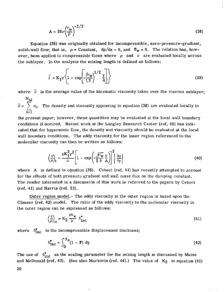
- 1/2 A = 26v(%)

Equation (38) was originally obtained for incompressible, zero-pressure-gradient, solid-wall flow; that is, p = Constant, dp/dx = 0, and PW = 0. The relation has, however, been applied to compressible flows where p and v are evaluated locally across the sublayer. In the analysis the mixing length is defined as follows:

where 6 is the average value of the kinematic viscosity taken over the viscous sublayer;

3 = 1 Vi. The density and viscosity appearing in equation (38) a r e evaluated locally in

the present paper; however, these quantities may be evaluated at the local wall boundary conditions if desired. cated that for hypersonic flow, the density and viscosity should be evaluated at the local wall boundary conditions. The eddy viscosity for the inner region referenced to the molecular viscosity can then be written as follows:

Nsz

i= 1

Recent work at the Langley Research Center (ref. 40) has indi-

where A is defined in equation (38). Cebeci (ref. 41) has recently attempted to account for the effects of both pressure gradient and wall mass flux on the damping constant. The reader interested in a discussion of this work is referred to the papers by Cebeci (ref. 41) and Harris (ref. 23).

Outer region model.- The eddy viscosity in the outer region is based upon the Clauser (ref. 42) model. The ratio of the eddy viscosity to the molecular viscosity in the outer region can be expressed as follows:

where 6Tnc is the incompressible displacement thickness;

6 x c = Joye(l - F) dy

The use of 6znc as the scaling parameter for the mixing length is discussed by Maise and McDonald (ref. 43). (See also Morkovin (ref. 44).) The value of K2 in equation (41)

20

is taken t o be 0.0168 as reported in reference 45. However, in order to account for the intermittent character of the outer layer flow, equation (41) is modified by an intermittency factor obtained by Klebanoff (ref. 46); that is,

where the transverse intermittency factor y(y) is defined as

1 - e r f [ 5 6 - 0.781

2 j7= (44)

The boundary-layer thickness normal to the wall boundary where

6 appearing in equation (44) is defined as the distance F = 0.995.

Matching procedure.- - The cr i ter ia used to determine the boundary between the inner and outer regions is the continuity of eddy viscosity. distribution is presented in figure 4.

A sketch of a typical eddy viscosity

E

Figure 4.- Matching procedure f o r two-layer model.

The matching procedure may then be formally written as follows:

P K ~ U ~ * - (& = 7 6inc 7

The location of the boundary separating the two regions ym is determined from the continuity of equations (45); that is, where

21

I

Eddy conductivity.- The eddy conductivity is formulated in te rms of a static turbulent Prandtl number Npr , t and the eddy viscosity E . (See eqs. (9) to ( l l ) . ) The two- layer concept for the eddy viscosity model suggests that there should also be a two-layer model for the static turbulent Prandtl number. Numerous assumptions have been made over the past years concerning the eddy conductivity, and corresponding models have been proposed to attempt to predict the mean turbulent boundary-layer temperature profiles. One of the earliest assumptions that has been used extensively is that the static turbulent Przhdtl number is a constant equal to unity and implies that the heat and momentum are transferred by the same process. However, the data which a r e available, although often inclusive, definitely show that N p r t is a function of y/6 for both incompressible and compressible flows. Consequently, the assumption of Npr , t = 1 would be expected to lead to e r ro r in predicting the temperature profiles for the turbulent boundary layer.

The incompressible data which are available for the outer region of pipe flow (ref. 47) and boundary layers (ref. 48) indicate that Npr,t ranges between 0.7 and 0.9. These data indicate that as the wall is approached, Npr,t achieves a maximum value near the wall and then decreases rapidly to a value between 0.5 to 0.7 at the wall. (See also ref . 49.) Simpson, Whitten, and Moffat (ref. 50) found that N p r , t ranged from approximately 0.95 at (y/6) = 0.1 to 0.45 at (y/6) = 1.0. The data in this region were predicted well by the expression Npr , t = 0.95[1 - 0.5(y/6)q as proposed by Rotta (ref. 51). which accounts for pressure gradient and mass transfer at the wall boundary. The resulting NPr ,t distribution appears to agree with both the experimental data of Simpson, Whitten, and Moffat (ref. 50) as well as with the Jenkins model (ref. 53). For compressible flows, where very little data are available, it appears that Npr , t has a value near unity in the outer region of the boundary layer and a value between 0.7 and 0.9 at the wall boundary (ref. 49). Rotta (ref. 51) found that Npr,t may reach values as high as 2.0 as the wall is approached before decreasing rapidly to the wall boundary value. Meier and Rotta (ref. 54) found for 1.75 5 M, 5 4.5 that N p r , t increased above unity for y+ < 50 and ranged between 0.8 and 0.85 as the outer edge of the boundary layer was approached.

Cebeci (ref. 52) presents a continuous expression for the eddy conductivity

The eddy conductivity and resulting static turbulent Prandtl number model must of necessity at the present time be formulated in te rms of existing experimental data. The assessment of the value of the current empirical models must be based upon the agreement between experimental and calculated temperature profiles over a wide range of flow variables. The inconclusiveness of much of the experimental data which exist to date for

22

both subsonic and supersonic flows and the lack of data for hypersonic flows clearly indicates the severe need for accurate, well-documented experimental temperature and velocity profile data. In the present analysis, since the cases considered deal specifically with either wall gradient values or velocity profile parameters, a constant Npr,t equal to 0.9 is utilized. However, the numerical procedure utilized is completely general and any function Npr,t(y/G)

sections has implied that K1, K2, and A+ (A' = A U , , ~ / V ~ ) a r e constants (see eqs. (45)) and therefore independent of flow conditions. However, recent studies have shown that K1, K2, and A+ a r e strong functions of Re,e fo r moderate to low Reynolds numbers; for example, Re,e < 5000. has found that a K1 able in predicting the velocity profiles in the law-of-the-wall region provided that Re,@ > 6000. Cebeci, using the data of Simpson (ref. 56), generated polynomial curves for K1 and A+ as functions of Re,e. These functions were then used to obtain predictions for the data of Whitten (ref. 57) which were in very good agreement in the law- of-the-wall region for strong function of Reynolds number for Re,e < 5000; that is, K2 ranges from a value near that used in the present analysis for Re,e > 5000 to values as large as 0.036 for

could be used.

____ Reynolds number effects.- The eddy viscosity model as presented in the previous

(See refs. 52 and 55.) Cebeci (ref. 52) value of 0.4, as used in the present analysis, is accurate and reli-

1200 5 Re,e 9 4100. McDonald (ref. 55) has shown that K2 is a

Re,e = 450.

For all the cases presented in the present paper, K1, K2, and A+ a r e held constant and equal to 0.4, 0.0168, and 26, respectively, since low R considered. However, the flexibility of the numerical technique allows any desired variation of these variables to be easily incorporated into the solution.

cases a re not e,e

Transformed models.- Since the governing equations are solved in the transformed plane, it is necessary to transform the eddy viscosity relations from the real plane t o the transformed plane.

In the inner region the ratio of eddy viscosity to molecular viscosity is as follows:

where y is defined by equation (31). The parameter II appearing in equation (47) is the damping t e rm and is defined as

II = 1 - exp(-nlH2) where

' l l l l I l l I l l 1

(49)

23

and

In the outer region the ratio of eddy viscosity to molecular viscosity is as follows:

where 1 - erf 5($ - 0.78)

2 r =

and

Transition Region

Equations (25), (26), (27), and (29) together with the boundary conditions (eqs. (32)), and the eddy viscosity relations defined by equations (47) and (51) complete the required system for either laminar or fully developed turbulent boundary-layer flows. However, the main objective is to present a technique that will efficiently solve the laminar, transitional, or turbulent boundary-layer equations as the boundary layer develops along the surface. Consequently, the location of transition ~ t , ~ , the extent of the transitional flow

xt,f - xt,i, must be taken into consideration.

and the characteristics of the mean flow structure in the transition region

Stability and transition.- Stability theory cannot currently be used to predict either the nonlinear details of the transition process after the two-dimensional waves have been amplified or the location of transition Stability theory can, however, establish the unstable boundary-layer profiles and the initial amplification rates. The theory can identify those frequencies which will be amplified at the greatest rate as well as the effect on stability of various flow parameters. (See refs. 2 , 58, and 59.) A review of methods used to predict the location of transition from stability theory is presented by Jaffe, Okamura, and Smith in reference 60. However, the connection, if any, between' stability and transition has not yet been established.

3 . . J

Transition location. - Many parameters influence the location of transition. These parameters can best be thought of as forming a parameter phase space. Such a parameter phase space would include Reynolds number, Mach number, unit Reynolds number,

24

surface roughness, nose bluntness, pressure gradients, boundary conditions at the wall., angle of attack, free-stream turbulence level, and radiated aerodynamic noise. Morkovin (ref. 12) recently completed a very extensive and thorough examination of the current state of the art of transition from laminar to turbulent 'shear layers. The most striking conclusion that one obtains from the review is that although a great bulk of experimental data on transition currently exists, much of the information on high-speed transition has not been documented in sufficient detail to allow the separation of the effects of these multiple parameters on transition. A discussion of the effects of each of the param- e te rs that may influence transition in high-speed flow is beyond the scope of the present paper.

The reader interested in a detailed discussion is directed to the paper by Morkovin (ref. 12) where over 300 related references a r e cited and discussed. Another, although l e s s detailed discussion, is presented by Fischer (ref. 61). The effects of radiated aerodynamic noise on transition a r e discussed by Pate and Schueler (ref. 62). Hypersonic transition, to name but a few references, is discussed by Softley, Graber, and Zempel (ref. 63), Richards (ref. 64), Potter and Whitfield (ref. 65), and Deem and Murphy (ref. 66). A discussion on the effects of extreme surface cooling on hypersonic flat- plate transition is presented by Cary (ref. 67). The effects of nose bluntness and surface roughness on boundary-layer transition a r e discussed by Potter and Whitfield (ref. 68). In the present analysis the location of transition will be determined by one of, or a com- bination of, the following three methods. These methods are (1) use of a stability index o r vorticity Reynolds number first proposed by Rouse (ref. 69), (2) use of correlations based upon a collection of experimental data over a broad range of test conditions, and (3) use of the measured experimental location of transition as a direct input into the analytical solution.

Stability index.- Hunter Rouse (ref. 69) nearly 25 years ago obtained by dimensional analysis a stability index expressed as follows:

This index has the form of a vorticity Reynolds number which is obtained from the ratio of the local inertial s t r e s s py2( ~ U / L ) Y ) ~ to the local viscous stress p( aU/8y). Rouse assumed that for transition to occur the stability index should reach some limiting value which was assumed to be invariant. He was able to show further that this invariant value

should be on the order of 500 for incompressible flows. (Xmm)cr The use of xmm as a stability index is in principle similar to the basic reasoning

which led 0sborn.e Reynolds (ref. 31) to postulate that the nondimensional parameter ud/v could be used to define a critical value (ud/v),, at which transition would occur in a

25

1

circular pipe of diameter d. Unfortunately, (xmax>pr is a function of the transition parameter phase space in much the same fashion as the critical Reynolds number and cannot in reality be a t rue invariant for transition as suggested by Rouse. The stability index does , however, possess a number of important characteristics which can be directly related to the stability of laminar flows.

A schematic distribution of x for a compressible laminar boundary layer is presented in figure 5.. The vorticity Reynolds number has a value of zero at the wall and approaches zero as the outer edge of the layer is approached. x, that is, xmax, occurs at some transverse location (y/6) The values of xmax and (Y/Qxmax are of importance in the use of the vorticity Reynolds number as a guide to boundary-layer stability and transition.

The maximum value of

Xmax'

As the laminar boundary layer develops over a surface, xmax increases mono- tonically until the critical value ( x ~ ~ ) ~ ~ is reached at which point transition is assumed to occur; that is, the location of ~ t , ~ . For compressible flows (xmax),, is not an invariant. In the present study ( x ~ ~ ) ~ ~ ranged from approximately 2100 to values on the order of 4000. The variation (x,,),, Reynolds number for data obtained in air wind-tunnel facilities. However, although not invariant, the stability index does exhibit the same dependence on various parameters that is predicted by the more complicated stability theory. streamwise location x, the value of xmax for supersonic flow is found to decrease (which implies a more stable flow) with wall cooling, wall suction, and favorable pressure gradients, whereas it increases (which implies a more unstable flow) with wall heating, mass injection (transpiration), and adverse pressure gradients. The vorticity Reynolds number appears to have been used as a correlation parameter in only two boundary-layer transition studies. A modified form of the parameter was used to

is a strong function of unit

For example, at a given

xm,

0 X

Figure 5.- Vorticity Reynolds number.

26

I

correlate the effect of free-stream turbulence on transition by Van Driest and Blumer (ref. 70). Correlation attempts, using Rouse's original invariant assumptions , were made by Ivensen and Hsu (ref. 71); however, the results were only fair.

One of the most important characteristics of the vorticity Reynolds number is that the value of ( Y / G ) ~ ~ = is in excellent agreement with the experimental location of the critical layer which represents the distance normal to the wall where laminar flow break- down will occur. Stainback (ref. 72) computed the Rouse stability index for s imilar laminar-boundary-layer flows over a broad range of. ratios of wall temperature to total temperature for Mach numbers up to 16. The numerical calculations were made for both air and helium boundary layers. The agreement between (y/6) and the experi- Xmax mental critical layer position was excellent over the entire range.

Empirical correlations.- In most instances one has to rely on empirical correla- :ions of experimental transition data in order to f i x the most probable transition location !or a design configuration. However, caution should always be used when obtaining the nost probable location of transition from such correlations, since any given correlation s based upon a specific collection of data which will not be completely general. There :urrently exists a number of empirical correlations for predicting the probable location )f transition. Some of these correlations a r e of questionable value; however, some can )e used with confidence providing it is realized that one is predicting a probable range if locations and not an exact fixed point. One of the more successful correlations unpublished) was obtained by Stainback and Beckwith for sharp cones at zero angle of tttack. The correlation is based on experimental transition data obtained over a wide range of test conditions in air wind tunnels, ballistic ranges, and free flight. The correla- ;ion can be expressed as follows:

lOg10(%) = P + QMe(Ow) 0.7 exp (-0.0 5 M 3

RF,d (55)

and Re 6* a r e the Reynolds numbers based on base diameter d and the e,d ' t

where R

displacement thickness at transition, respectively. The constants P, Q, and R a re functions of the environment in which transition was measured and are given in the following table:

Ballistic range Free flight 1.2683 .lo441 .325

27

Equation (55) can be expressed follows:

in t e rms of the transition Reynolds number Re as 3% ,i

+ 2QMe(Ow) 0.7exp( -0.05Mz)j

2 (0.094Mz + 1.220,)

Equations (55) and (56) a r e s imilar t o the relations presented by Bertram and Beckwith (ref. 73); however, the constants P, Q, and R presented in the preceding table a r e somewhat different from those of reference 73.

Experimental transition.- Much of the confusion that exists in the literature concerning boundary-layer transition may be attributed to the following two factors. The first factor is that in many instances the investigator who made the experimental study may not have carefully measured or recorded the complete conditions under which the data were obtained. The second factor is that the experimentally observed transition location depends on the experimental technique used.

The importance of carefully measuring the environment under which the experiments a r e made cannot be overstressed. In the past, many of the factors which influence transition such as free-stream turbulence and acoustic radiation from the tunnel side- wall boundary layer were not measured. (See refs. 73 to 76.) The location of transition as obtained experimentally is a function of the method used to determine its location. There a r e currently a number of techniques used to obtain the transition location. Some of these methods a r e hot-wire t raverses , pitot-tube surveys near the wall, visual indication from schlieren photographs, and heat-transfer measurements at the wall. Each of these methods basically measures a different flow process. Consequently, it would be misleading to believe that each technique would yield the same location for transition if simultaneously applied to the same boundary layer. Of course, the concept of a transition rlpoint'' is misleading in itself since transition does not occur at a "point" but instead over some finite region.

For the test cases presented herein, the transition location % . 9 1 from heat-transfer measurements at the wall whenever possible. The reason for this choice is that it is the method most often used in the literature. However, it should be noted that the actual nonlinear transition process begins somewhat upstream of the location where the heat transfer at the wall deviates from the laminar trend.

will be determined

Transitional flow structure.- Once the transition location has been fixed for a given problem, one must next consider the following two important factors; first, the length of the transition region, %,f - xt!i (sometimes referred to as transition extent), and sec- ondly, the mean flow characteristics within the region. Once appropriate models a r e

28

obtained for these two factors, it is possible to connect the three flow regions smoothly so that one set of governing equations may be used.

The laminar boundary-layer equations (eqs. (1) to (3)) should yield accurate profiles and wall boundary gradients in the region prior to turbulent spot formation. The intermittent appearance of the turbulent spots and the process of cross-contamination are not well understood. The spots originate in a more or l e s s random fashion and merge with one another as they grow and move downstream. Eventually, the entire layer is con- taminated which marks the end of the transition process As the turbulent spots move over a fixed point in the transition region, the point experiences an alternation between fully laminar flow when no spot is present and turbulent flow when engulfed by a spot. These alternations can be described by an intermittency factor which represents the fraction of time that any point in the transition region is engulfed by turbulent flow.

3 Yf '

The distribution of spots in time and space is Gaussian for low-speed natural transition. However, very little is known about the spot distribution in high-speed compressible flow. Furthermore, there is no assurance that the spot formation and distribution in hypersonic flows will be analogous to the low-speed model; however, in the absence of a more satisfactory theory, the approach of Dhawan and Narasimha (ref. 77) is used. In reference 77 the source density function of Emmons (ref. 20) w a s used to formulate the probability distribution (intermittency) of the turbulent spots as follows:

where

- %,i 5 =

fo r 5 5 x S . The t e rm 5 in equation (57) represents a normalized streamwise coordinate in the transition region, and h is a measure of the extent of the transition region; that is,

Y 3 ,f

The intermittency distributions in the transverse direction (y-direction) a r e similar to those observed by Corrsin and Kistler (ref. 78) for fully developed turbulent boundary layers (ref. 79). Corrsin and Kistler found that the transverse intermittency varied from a maximum of unity near the wall to a near-zero value at the outer edge of the layer. The transverse intermittency distribution is of secondary importance in relation to the streamwise distribution in determining the mean profiles and wall fluxes; consequently, the only intermittency distribution applied in the transverse direction (y-direction) is that of Klebanoff (ref. 46) in the outer layer as applied to the fully developed turbulent layer. (See eq. (44).) It should be carefully noted in order to avoid any confusion concerning the

29

two intermittency functions used herein that r is a function only of the x-coordinate whereas 7 is a function only of the y-coordinate.

Transition extent. - The assumption of a universal intermittency distribution implies that the transition zone length (transition extent) can be expressed as a function of the

transition Reynolds number u ~ % , ~ e. In reference 77 it is shown, for the transition data considered, that the data are represented on the average by the equation

l'

can then be obtained ue ue xt ,f

where R e , b t = - Axt.

directly from equation (60) as follows:

The location of the end of transition

xt,f = xt,i + 5Ri1(R e 9% ,i )OB8 where Re is the local unit Reynolds number ue/ue. Morkovin (ref. 12) noted that only about 50 percent of the experimental data he considered could be fitted to the low-speed universal curve of Dhawan and Narasimha, that is, to equation (60). This result was to be expected, since the data considered in reference 77 covered only a very limited Mach number range.

Potter and Whitfield (ref. 68) measured the extent of the transition zone over a rather broad Mach number range (3 2 M, 2 5; tion region, when defined in t e rms of Re,Axt, is basically independent of the unit Reynolds number and leading-edge geometry; that is,

= 8). They observed that the transi-

Re,A% = S2R ( e,%,i) "m)

They noted (ref. 68) that the extent of the transition region increased with increasing transition Reynolds number over the Mach number range 0 S M, 5 8 for adiabatic walls. The extent of the transition region was also observed to increase with increasing Mach numbers for a fixed transition Reynolds number.

In the present analysis, because of the lack of general correlations for the extent of transition, this quantity is obtained directly from the experimental data unless otherwise noted. In particular, if heat-transfer data a re available, the transition zone is assumed to lie between the initial deviation from the laminar heat-transfer distribution and the final peak heating location. The transition region defined on the basis of the Stanton number distribution is presented in figure 6. The design engineer seldom has the advantage of having access to experimental data which were obtained under the actual flight conditions. Consequently, the most probable location of transition would be obtained from a

30

Laminar 4- Tronsitionol --/--Turbulent

, \ +

L R%Xt,f I

Loco1 Reynolds number, Re,x

Figure 6.- Transit ion ex ten t def in i t ion .

correlation such as presented in equation (56). The extent of transition could then be obtained from equation (61) or an approximate relation such as follows (see ref. 80):

NUMERICAL SOLUTION OF THE GOVERNING EQUATIONS

The system of governing equations for compressible laminar, transitional, and turbulent boundary layers consist of three nonlinear partial differential equations (see eqs. (25). to (27)) and two algebraic relations. tant feature of this system is that it is parabolic and therefore can be numerically integrated in a step-by-step procedure in the streamwise direction. In order to cast the equations into a form in which the step-by-step procedure can be efficiently utilized, the derivatives with respect to 5 and q are replaced by linear finite-difference quotients.

The method of linearization and solution used in the present analysis closely paral-

(See eqs. (17) and (18).) The most impor-

lels that of FlGgge-Lotz and Blottner (ref. 29) with modifications suggested by Davis and

three-point implicit differences in the [-direction which produce truncation e r r o r s of order A t 1 A52 rather than Ax as in reference 29. The primary difference between the present development and that of reference 30 is that the solution is obtained in the transformed plane for arbi t rary grid-point spacing in the (-direction and for a spacing in the q-direction such that the ratio of the spacing between any two successive grid points is a constant.

1 Fliigge-Lotz (ref. 30) to improve the accuracy. These modifications involve the use of

31

The Implicit Solution Technique

Finite-difference mesh model.- It has been shown for laminar boundary layers that equally spaced grid points can be used in the normal coordinate direction. (See refs. 29 and 30.) However, for transitional and turbulent boundary layers, the use of equally spaced grid points is not practical because the fine-mesh size required to obtain accurate results near the wall boundary is inefficient for the entire boundary layer. The grid- point spacing in the q-direction used in the present analysis assumes that the ratio of any two successive steps is a constant; that is, the successive Aqi form a geometric pro- gression. (See ref. 81.)

The advantage of having variable grid-point spacing in the x-coordinate becomes clearly apparent for problems in which either the rate of change of the boundary conditions is large or discontinuous o r the mean profiles are changing rapidly. A good example would be a slender blunted cone in supersonic flow. Variable grid-point spacing in the ,$-direction would be utilized by having very small steps in the stagnation region where the pressure gradient is severe (favorable) and again in some downstream region where transitional flow exists. A good example of discontinuous boundary conditions would be a sharp-tipped cone with a porous insert at some downstream station through which a gas is being injected into the boundary layer. Relatively large step s izes could be utilized upstream of the ramp injection; however, small steps must be used in the region of the ramp injection. Downstream of the porous region, as the flow relaxes, larger step sizes could be used. It is very important that small grid-point spacing be utilized in the transition region where the mean profiles a re a strong function of the intermittency distribution.

In constructing the difference quotients, the sketch of the grid-point distribution presented in figure 7 is useful for reference. The dependent variables F, 0, and V are assumed to be known at each of the N grid points along the m - 1 and m stations, but unknown at station m + 1. The A51 and A t 2 values, not specified to be equal, a r e obtained from the specified x-values x ~ - ~ , Xm, and x ~ + ~ ) and equation (20a). The relationship between the lowing equation:

( Aqi for the chosen grid-point spacing is given by the fol-

Aqi = (K)i-l (i = 1, 2, . . ., N) (64)

where K is the ratio of any two successive steps, Aql is the spacing between the second grid point and the wall (note that the first grid point is at the wall boundary), and N denotes the total number of grid points across the chosen q-strip. The total thickness of the r]-strip can then be expressed as follows:

32

N -

N - I -

n+t -

n -

n-1 -

6-

5-

4-

3- 2-

i = l -

~

__ I I I I I I I I I I I I -_ ~

I

t I

I I I

I I I I I -

_.

Figure 7.- Finite-difference grid model.

The selection of the optimum K and N values for a specified qN depends upon the particular problem under consideration. The main objective in the selection is to obtain the minimum number of grid points with which a convergent solution may be obtained and thereby minimize the computer processing time per test case. The laminar boundary layer presents no problem since a K value of unity is acceptable; however, for transitional and turbulent layers, the value of K will be a number slightly greater than unity, for example, 1.02 to 1.04. If transitional o r turbulent flow occurs in a given problem; the laminar part of the boundary layer is calculated with the value of K used for the turbulent region; that is, for a given problem K is invariant.

Difference equations.- Three-point implicit difference relations (see appendix A) are used t o reduce the transformed momentum and energy equations (eqs. (26) and (27)) to finite-difference form. The difference quotients produce linear difference equations when substituted into the momentum and energy equations provided that truncation t e rms

33

I1 I1 I l l IIIIII 11l11ll11l11ll~11111111lllllI

of the order A t m - l Atm and Aqn-l Aqn are neglected. The resulting difference equations may be written as follows:

The coefficients An (1) ,Bn (1) , . . ., ($1) , Ai2), . . .,Gf) (see appendix B) a re functions

of known quantities at stations m and m - 1. The dependent variable V does not appear explicitly as an unknown at station m + 1 This condition occurs because of the particular way that the nonlinear te rms and V(aO/aq) appearing in the momentum and energy equations (eqs. (26) and (27)), respectively, are linearized (see eq. (A23)); however, equations (66) and (67) a r e coupled in that the dependent variables F and 0 appear explicitly in each equation.

in these equations (eqs. (66) and (67)).

V( aF/aq)

Solution of difference equations.- The system of difference equations (eqs. (66) and (67)) represents a set of exactly 2(N - 1) equations for 2(N - 1) unknowns since the N - 1 unknown values of V do not appear explicitly and the Ail),Bil), . . n coefficients a r e known. The proper boundary conditions to be used with the difference equations a r e specified in equations (32). The system of algebraic linear equations may be written as a tridiagonal matrix; consequently, an efficient algorithm is available for their simultaneous solution. The simultaneous or coupled-solution technique has been discussed in detail by FlGgge-Lotz and Blottner (ref. 29). tems where only two governing equations must be considered, the simultaneous solution technique (coupled solution) is very efficient since the equations a r e solved without the need for iteration procedures such as in reference 33. However, for real-gas flows or systems where more than two governing equations a re required, the iterative (uncoupled) solution technique proposed by Blottner (ref. 6) should be used to avoid the large digital computer storage requirements associated with the present coupled solution technique. Another uncoupled solution technique that appears to be more flexible and faster than the method presented in reference 6 is that developed by Keller and Cebeci (ref. 82). This method should efficiently handle both three-dimensional steady and two-dimensional

GO)

For perfect gas flows o r sys-

34

unsteady flows as well as flows with chemically reacting species; however, the technique to date has not been used extensively.

Solution ~ ~~ of continuity equation.- The continuity equation (eq. (25)) can be numerically solved for the N - 1 unknown values of V at station m + 1 once the values of F and 0 are known at station m + 1. Equation (25) is integrated to yield the following relation for V at the grid point (m + 1, n):

m+l -

'm+l,n - 'm+1,1

represents the boundary condition at the wall and is defined in equa- where 'm+1,1 tion (34) as a function of the mass transfer at the wall (pv),. The integral appearing in equation (68) is numerically integrated across the v-strip to obtain the N - 1 values of V. In the present analysis, the trapezoidal rule of integration was utilized; however, any sufficiently accurate numerical procedure could be used.

Initial profiles.- Initial profiles for starting the finite-difference scheme a r e required at two stations since three-point differences a r e utilized. The initial profiles at the stagnation point or line for blunt bodies, o r near x = 0 for sharp-tipped bodies, a r e obtained by a numerical solution of the similar boundary-layer equations. The equations a r e solved by a fourth-order Runge-Kutta scheme with a Newton's iteration method to modify the initial estimates of the gradients of F and 0 evaluated at the wall boundary. The N-1 values of F, 0, and V which a r e now known at the N - 1 equally spaced grid points a r e numerically redistributed to N - 1 grid points whose spacing is determined from equations (64) and (65), if a variable spacing is required. The second initial profile located at station m is assumed to be identical t o the one located at station m - 1. Any e r r o r s that might be incurred because of this assumption a r e minimized by using an extremely small A t , that is, an initial step s ize in the physical plane on the order of Ax = 1 X The solution at the unknown station m + 1 is then obtained by the finite-difference method. Extremely small, equally spaced At-steps a re used in the region of the initial profile. The step s ize is increased after the e r r o r s due to the starting procedure have approached zero, that is, after 10 to 15 steps in At.

It is also advantageous to have the capability of starting the solution from experi-

can be directly incorporated into the numerical procedure used in the present analysis. This capability is extremely useful for cases where one cannot easily locate the origin of the boundary layer, f o r example, on nozzle walls.

I mentally measured profiles, especially in the case of turbulent flow. This capability

Evaluation . - of wall derivatives.- The shear stress and heat transfer at the wall are

By using G to represent a general quantity where Gm+l,l is not specified t o be zero,

_ - I directly proportional to the gradient of F and 0 evaluated at the wall, respectively.

I

35

the four-point difference scheme used to evaluate derivatives at the wall is as follows (see pp. 49 to 50, ref. 29):

($)m+l ,I= Y7Gm+1 ,1 + Y8Gm+1 ,2 + Y9Gm+1 ,3 + YIOGm+l ,4

where the coefficients Y7, . . ., Yl0 are defined by the following relations:

(1 + K + K2l2h(1 + K) - 13 + 1 + K Y7 = -

(1 + K)(1 -I- K + K2)K3Aq1

1 + K + K 2 Y - - - (1 + K)K3Aq1

1

ylo = (1 + K + K2)K3Aal J For the case of equally spaced grid points in the q-direction (K = l), equations (70)

become

9

and equation (69) reduces to the four-point relation (see pp. 49 t o 50, ref. 29); that is,

Eddy Viscosity Distribution

The primary difference between the present solution technique and other typical procedures such as those of Cebeci, Smith, and Mosinkis (ref. 83) and Beckwith and

36

Bushnell (ref. 84) is that the momentum and energy equations (eqs. (66) and (67)) a r e simultaneously solved without iteration, whereas in the techniques of these two references the momentum and energy equations are each individually solved and iterated for convergence. In the present procedure, extreme care must be used when the eddy viscosity functions E' and ? (see eqs. (15) and (16)) and their derivatives with respect t o 7 are extrapolated from the known values of Em-l,n and Em,n to the unknown station m + 1, n.

During the development of the present digital computer program, the calculations would frequently become unstable in either the transitional o r turbulent flow region. This problem would always occur in one of two ways. In some instances an apparently converged solution would be obtained, but the distribution of boundary-layer thickness would not be smooth. In other instances, where the transition was abrupt or where bound- a ry conditions were abruptly changed, the solution would not converge. The problem was caused by a wavy or rippled distribution in eddy viscosity across the layer. These ripples first occurred in the region where the inner and outer eddy viscosity models were matched. If the initial ripples were below a certain level, the solution would apparently converge, but slightly nonsmooth boundary-layer thickness distributions would occur. If the initial ripples were above a certain level, the oscillations would grow very rapidly as a function of 5 and propagate throughout the layer as the solution proceeded down- s t ream with the result that valid solutions could not be obtained downstream of the initial ripples.

and 'm-l,n to the unknown m,n The initial extrapolation of the known values of E' grid point (m + 1, n) is obtained as follows (see eq. (A3)):

However, there is no assurance that the distribution of the extrapolated values at station m + 1 will be smooth across the layer for all possible flow conditions. If oscillations occur in the extrapolated E' distribution of sufficient magnitude to cause the sign of the derivative of with respect to q to alternate, then the entire calculation becomes highly unstable.

4 The requirement of small grid-point spacing in the law-of-the-wall region con- tributes to the stability problem since the size of an "acceptable oscillation" is apparently

where the viscous sublayer is relatively thick, the grid-point spacing in the outer portion of the law-of-the-wall region will be large in comparison with cases where the viscous sublayer is relatively thin. Consequently, the former case can tolerate a larger ripple in the region of the match point

3 a function of the grid-point spacing being utilized in the 7-direction. For turbulent layers

I

~

1 change in the sign of the derivative of E with respect to 7. I ym than can the latter case without experiencing a j

I

37

There a r e two possible ways to eliminate the problem caused by the oscillations in the eddy viscosity distribution. The first approach is to develop an iteration scheme; in which case the present solution technique has no advantage over other techniques (for example, refs. 33, 83, and 84), that is the advantages of the simultaneous solution would be lost. The second approach is to smooth numerically the extrapolated eddy viscosity distribution prior to the matrix solution. Both approaches were tr ied during the development phase of the digital computer program. The second approach was incorporated into the solution and is discussed in the remaining part of this section.

The problem posed by the ripples in the eddy viscosity distribution, if they exist, can be avoided by utilizing a three-point mean value for at station m + 1, n; that is,

where Eav denotes the three-point mean of the eddy viscosity function. In the present procedure the eddy viscosity functions appearing on the right-hand side of equation (74) are first obtained at each grid point across the m + 1 station from equation (73). After these values a r e obtained, the three-point mean is evaluated at each of the N - 1 grid points from equation (74). The matrix solution for F and 0 is then obtained for equations (66) and (67) by using these precomputed values of (Eav)m+l,n. After the N - 1 values for F, 0, and V at station m + 1 have been obtained, the eddy viscosity distribution is recalculated at the m + 1 station from equations (47) and (51) prior to moving to the next 5 grid-point station. This procedure has been found to be stable under all circumstances and to yield convergent solutions for transitional and fully turbulent boundary layers.

EXAMPLE SOLUTIONS AND COMPARISONS WITH

EXPERIMENTAL DATA

The selection of a typical set of test cases always presents a problem since there a r e many possibilities from which to choose. However, the cases considered in the present paper were chosen to provide an indication of the meri ts of the solution technique as well as the validity of the eddy viscosity and intermittency models. In all cases presented herein, the gas is assumed to be perfect air with a constant ratio of specific heats (y = 1.4), a constant Prandtl number ( N p r = 0.72), and a constant static turbulent Prandtl number (Npr,t = 0.9). The molecular viscosity p is evaluated from Sutherland’s viscosity law (eq. (18)). The external pressure distributions used a r e either experimental or obtained from an exact solution of the full inviscid Euler equations. All calculations were made on the Control Data Corporation 6600 digital computer.

38

Flows with large adverse pressure gradients are not considered in the present paper. This omission is due to the current lack of understanding of the effect of large adverse pressure gradients on the turbulent models for supersonic flow as discussed by Harr is (ref. 23) and Beckwith (ref. 17) who have made comparisons of numerical results with the experimental data of McLafferty and Barber (ref. 85).

High Reynolds Number Turbulent Flow

The accurate prediction of boundary-layer characteristics for high Reynolds number turbulent flow is important in the design of high-speed vehicles. In particular, it is important to be able to predict with accuracy the skin-friction drag. A good example of high Reynolds number turbulent flow is provided by the data of Moore and Harkness (ref. 86). The experimental skin-friction data were measured with a floating-element- type balance. The data were obtained on a sharp-leading-edge flat-plate model that completely spanned the width of the tunnel test section for 1 X lo7 < Re,x < 2 X lo8 and on the tunnel diffuser floor for 2 X lo8 < Re,x < 1 X lo9. The tes t conditions were as follows:

M, = 2.8

Pt,, = 0.997 MN/m2

Tt,, = 311.1 K

m L W - = 0.947

Tt,,

The experimental transition location was not reported in reference 86. Conse- quently, for the numerical calculations, the transition location was determined by the stability index and was assumed to occur at the x-station where xmax achieved a value of 2500. The extent of the transition region was calculated from equation (61). The intermittency distribution was calculated from equation (57). The solution was started at the leading edge of the sharp flat plate (x = 0) by obtaining a numerical solution of the similar boundary-layer equations. (See eqs. (B47) to (B49) .) The grid-point spacing was varied in both the 5 - and ?-directions in order to check for convergence. i

The numerical results fo r the skin-friction coefficient distribution a r e compared with the experimental data in figure 8(a). The agreement is excellent over the entire Reynolds number range of the experimental data for K = 1.04; however, for K = 1.01, convergence was not attained. It should be noted at this point that the te rms convergence and stability, as used in relation t o the numerical method, are defined herein as in references 23 and 29. The divergence for K = 1.01 is attributed to an insufficient number of grid points in the wall region, in particular, in the thin viscous sublayer region.

t

I

~

1 39 I

d IIllIllllIlIllllllIlll111l1lllIlIllIllll1 I I I I

The effect of the grid-point spacing parameter K on the numerical solution was studied for additional values of 1.02, 1.03, 1.05, and 1.06. The solution was found to diverge for K < 1.02 and converge for K S 1.02. The Cf,e results for K 2 1.02 (other than K = 1.04) a r e not presented since the variation of Cf,e with K would not be discernible if plotted t o the scale of figure 8(a). The convergence criteria used in this particular example was to decrease the q-grid-point spacing until any change which occurred in Cf,e at a given x-solution station was beyond the fourth significant digit. The laminar curve shown in figure 8(a) was obtained by suppressing transition (r = 0). Grid-point spacing in the x-direction was varied from Ax = 0.03 t o 1.22 cm, and convergence to the accuracy of the experimental data was obtained for all values; because of the abruptness of transition, step s izes greater than Ax = 1.22 cm were not studied.

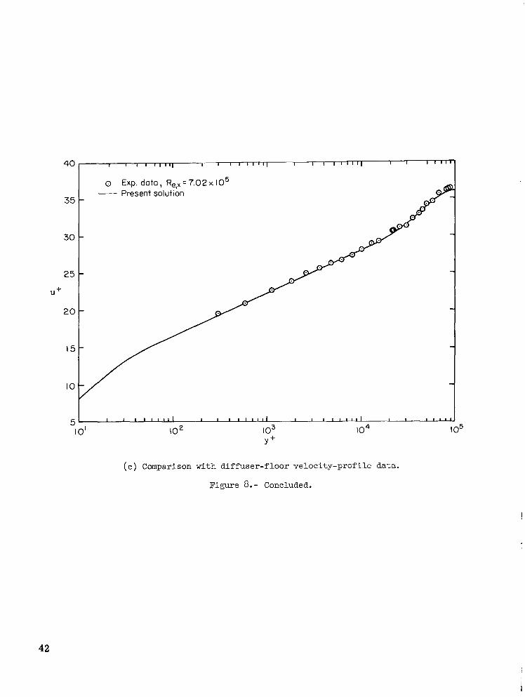
Comparisons of the numerical results with typical experimental velocity profiles a r e presented in figure 8(b) for the flat-plate model and figure 8(c) for the tunnel diffuser floor. The agreement is seen to be very good.

I I I I I I I I I I I 1 I I " I I I I I I I I I - - - Exp. doto -

0 Flat plote - El Diffuser floor -

Present solutions K.1.04 K =1.01 Lominor

i\ I \ - ' \

- ---- --

- - - - - -

. . \ \ . . \ .

L. - \. -

lo-2

C f,e

IO-^

IO-^

-I \ \.

.\. '. I I I I I I I l l I I I I I l I I 1 I l l 1 1

Re, x

(a) Comparisons with skin-friction coefficient data.

Figure 8.- High Reynolds number turbulent flow.

40

~ 1.- I - - r - - I

Exp. data, Re,, 8.45x107

Present solution, K = 1.04

0

1 I I J I I I I I

IO' IO2 I o3 lo4 Y +

(b) Comparison with flat-plate velocity-profile data.

Figure 8.- Continued.

41

40

I O

5 I

- Present solution

0' IO2 lo3 104 I o5 Y +

( c ) Comparison with diffuser-f loor veloci ty-prof i le data.

Figure 8.- Concluded.

42

Tripped Turbulent Boundary Layers

In most supersonic and hypersonic wind-tunnel facilities, it is necessary to t r ip the laminar boundary layer on small-scale models in order to simulate the full-scale conditions where most of the boundary layer would be turbulent. An example of turbulent data obtained by tripping the laminar boundary layer is that of Coles (ref. 87). These data were obtained in the Jet Propulsion Laboratory 20-inch supersonic wind tunnel. The test model was a sharp-leading-edge flat plate. The free-stream Mach number was varied from 1.966 to 4.544. Test numbers 30, 20, and 22 (see p. 33 of ref. 87) were selected as typical test cases. For these three cases the laminar boundary layer was tripped by a fence located at the leading edge of the flat plate. (See fig. 40 of ref. 87.) The skin friction was measured at three surface locations with a floating-element balance. Boundary- layer profiles were measured at x = 54.56 cm.

The test conditions for the three cases a r e listed as follows:

Pt," m / m 2

0.09468 .1373 .3894

Coles' test number

30 20 22

I T+, K Tw/Tt,m

302.8 0.8295 311.7 .7152 307.8 .6764

Me

1.982 3.701 4.554

-

Transition was assumed to occur near the leading edge of the plate for the numerical calculations % . = 0.15 cm and to be completed (I? = 1.0) at 3 f = 0.30 cm. Twenty

71 9 equally spaced x-solution stations were used in the region 0 5 x 5 0.30 cm; the x-solution stations were then equally spaced 0.30 cm apart over the remainder of the plate. The total number of grid points in the pdirect ion and the grid-point spacing parameter K were assigned values of 301 and 1.04, respectively. The computer processing time per test case was approximately 3 minutes. The numerical results a r e compared with the experimental velocity and Mach number profile data in figure 9 for the three test cases. The agreement between the numerical results and the experimental data is very good for all three test cases. In particular, it should be noted that the experimental skin- friction coefficients (see figs. 9(a), s ( ~ ) , and 9(e)) were predicted to within 1 percent, which is well within the accuracy range of 2 percent as quoted for the data in reference 87. The slight disagreement between the numerical results and the Mach number profiles for increasing free-stream Mach number may be due in part to eddy conductivity effects caused by the simple Npr, t model utilized in the calculations.

43

I .o

.6

F

! - Present solution 0.00202 (exp.) 0.00200 (Dredicted)

I I I I I 1 I I I I 0 2 4 6 8 IO 12 14 16 I8

Y / Q

(a) Velocity p r o f i l e and sk in- f r ic t ion coef f ic ien t f o r = 1.982.

0 EXP. doto; Me= 1.982

- Present solution

I I I I I I I I u

Y/8 0 2 4 6 8 IO I2 14 16 18

(b) Mach number p r o f i l e f o r M, = 1.982.

Figure 9.- Comparisons with experimental data f o r t r ipped turbulent boundary layers .

44

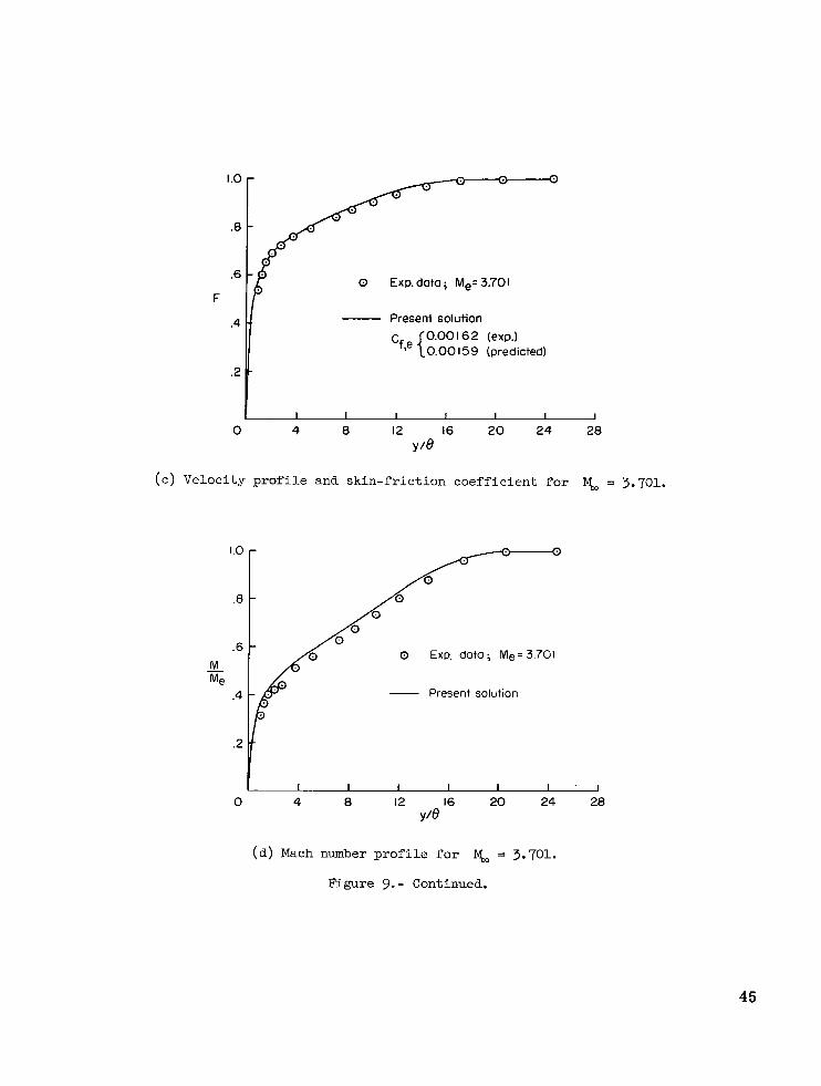
I .o

.8

.6

F

.4

.2

0

w w 0

I I 1 1 1

4 0 12 16 2 0 24 28 Y/8

(c) Velocity profile and skin-friction coefficient for % = 3.701.

1.0

.8

.6

.4

.2

0 Exp. doto ; Me= 3.701

Present solution 0.00 I 6 2 (exp.) 0.00 159 (predicted)

4 0 12 16 2 0 24 28 Y/8

Exp. data; Me= 3.701

- Present solution

I I 1 1 1 I ' I

0 4 8 12 16 20 24 28 Y/8

(d) Mach number profile for Ea, = 3.701.

Figure 9. - Continued.

45

I .o

.8

.6

F

.4

.2

- Present solution

0.00122 (exp.) 0.00 120 (predicted)

H I I 1 . I 1 1 . . L ~ I

Y / O 0 4 8 12 16 20 24 28

(e) Velocity profile and skin-friction coefficient for M, = 4.354.

I .o

.8

.6

.4

.2

Q Exp. data; Me-4 .554

- Present solution

I I I I 1 1 0 4 8 12 16 20 24

Y

(f) Mach number profile f o r Q = 4.554.

I -

28

Figure 9. - Concluded.

46

Laminar Flow With Mass Injection

An example of data for laminar flow with transpiration cooling is presented by Marvin and Akin (ref. 88). These data were obtained over a range of injection rates for a sharp-tipped 5O cone. The cone was solid for x c 9.53 cm; the remainder of the cone was porous. The test conditions were as follows:

M, = 7.4

Pt,.o = 4.137 N/m2

Tt,, = 833.3 K

TW -= 0.38 Tt ,,

The air-injection parameter a maximum value of 1.3903 X

F" ranged from a minimum value of zero (no injection) to

A comparison of the heating rate at the wall normalized by the heating rate at the wall just prior to the ramp injection (x = 9.53 cm) is presented in figure lO(a). The mass injection distribution was not uniform, as can be seen from the plot of the actual injection distribution normalized by the ideal injection rate. The nonuniform distribution of mass injection was utilized in the numerical solutions. The agreement between the numerical results and the experimental heat-transfer data is excellent over the entire injection range. Marvin and Sheaffer (ref. 89) have also obtained numerical solutions for this test case which a r e in very good agreement with the experimental data.

This particular case is an example where variable step size must be used in the region of the ramp injection (x/L = 1.0). For this case the Ax values (grid-point spacing in the x-direction) were constant and equal to 0.3 cm up to x/L = 0.99 at which point the step size was decreased to a value of 0.03 cm through the ramp injection region. The step size was then progressively increased up to a value of 0.3 cm at x/L = 1.5. The flow was laminar; consequently, K was set to unity and 101 equally spaced grid points were used in the q-direction. The digital computer processing time per test case was approximately 2 minutes.

The effect of mass injection on the vorticity Reynolds number is shown in figures 10(b) and lO(c). In figure 10(b) the maximum value of the vorticity Reynolds number xmax is seen t o increase with increasing x. In particular, the y/6 value at which xmax occurred is in excellent agreement with the location of the critical-layer position. (See ref. 72.) The effect of mass injection on the vorticity Reynolds number distribution is presented in figure lO(c). Increasing mass injection increases the value of xmax at a given x-station as well as moves the location at which the maximum occurs (Y/6) xmax toward the outer edge of the boundary layer.

47

I .4

1.2

1.0

.8 - 9, (qw )x - ,

L - .6

.4

.2

\ ^. F

0 0 El 3.823XlO-44 0 7.646XlO- \ A l .390xlo-3

Ideal distribution 10 r.. . . . . . . . . . . . . . . . . . . . . . . . . . . . . . . . . . . . . . . . . . . . . . .

8 t r i M e o s u r e d distrib

0 I 1 1 ~2

1 2 X/L

(a) Comparisons with heat-transfer data.

3

Figure 10.- Hypersonic laminar boundary-layer flow with mass injection.

48

------- - - _ _ _ _ _ _ _

y 8 Present solutions x/L " L F c$

Crit. loyer position 0.64 0 9.53 . . . . . Present solution

------ 0 Ref. 7 2

I I I I 1 I ! I 1 I I I 0 2 4 6 8 IO I2 14 16 I8 20 22 2 4 ~ 1 0 ~

X

(b) Vorticity Reynolds number distribution f o r zero mass injection.

- - - - -_____ -------- - - ---.: T,-,7 ~ . - , ~ ~ . . . . . . . . . . . . . . . . . . . . . . . . _ _ _ _ _ _ _ _ _ _ _ ---------- . . . . . __ - - - r _--

L, Present solutions F x/L cm Y

Crit. layer position 0 1.92 9.53

a Ref. 72 _ _ _ _ _ _ 1 . 3 9 0 ~ l O - ~

. . . . Present solution - 3.823X10-44 ~ _ _ 7646x10-

1 I I I I I I I 0 2 4 6 8 IO 12 14 16 18x103 I 1

X

(c) Vorticity Reynolds number distribution for variable mass injection.


49

Laminar Blunt Body Flow

The numerical procedure as presented in the present paper has been applied to a number of blunt-body flows at supersonic and hypersonic speeds. A typical case for a hemispherical nose is presented in figure 11. The test conditions for this case were as follows:

M, = 10.4

= 10.77 MN/m2 Pt,m rn = 0.08891 m

Tt,, = 1222 K

TW Tt,m -= 0.25

Solution for this particular example has been obtained by Marvin and Sheaffer (ref. 89) and Clutter and Smith (ref. 90). The heating rate and shear s t r e s s at the wall referenced t o the maximum heating rate and shear s t ress , respectively, a r e compared with the results presented in references 89 and 90 in figure 11.

Equally spaced grid points were used in the t-direction. Solutions were obtained fo r Ax values ranging from 0.03 cm to 0.60 cm in order to check for convergence.

I .o

.8

.6

.l.O

.8

.6

& (r")max

.4

.2

I I I I

x /cn

0 Ref. 89 I7 Ref. 90 - Present solution

I .4 .8 1.2

x/r, 1.6

Figure 11.- Hypersonic blunt-body flow.

50

The data shown in figure 11 were calculated by using Ax = 0.15 cm although much larger steps could be used for engineering calculations, for example, Ax = 0.3 cm. The grid- point spacing in the pdirect ion was held constant (K = 1).

Another example of hypersonic laminar flow is presented in figure 12. These experimental data were obtained on a spherically blunted, 25' half-angle cone. (See ref. 91.) ' The test conditions were as follows:

M,= 7.95

= 6.31 MN/m2 Pt,,

Tt,, = 783 K

. I

TW Tt,W -= 0.38

0

The pressure distribution used in the numer--al solu,ion was obtained by

7 1 I - 0 Data (ref. 91)

\ ' - -

I .o

.8

.6

.4

- pw

psp .3

.2

he techn .que presented in reference 92 and is compared with the experimental data in figure 12(a).

,-Tanq;t point Cone base 1 I 1 I I I I I I I 2 3 4 5 6 7 8 9 10 I 1

x/rn

( a ) E x t e r n a l p r e s s u r e d i s t r i b u t i o n .

F igure 12.- Laminar f low over a s p h e r i c a l l y b l u n t e d 25' h a l f - a n g l e cone.

51

x /rn

(b) Comparison w i t h heat-transfer data. rn = 0.10; d = 1.27 cm.

Figure l2. - Conciuded.

The numerical results fo r the heat-transfer coefficient distribution referenced t o the stagnation-point value are compared with the experimental data in figure 12(b) and also with the local similarity method as reported in reference 91. The present results are in somewhat better agreement with the data than the local similarity results presented in reference 91. In order to assess the difference between the two predictions, the present method was utilized as a local similarity method by eliminating the nonsimilar t e rms from the governing equations. (See eqs. (B47) to (B49).) The results of this solution a r e also shown in figure 12(b) and indicate that the discrepancies in the present nonsimilar solution and the local similarity solution presented in reference 91 a r e not due to the nonsimilar t e rms in the governing equations.

Nonsimilar Flow With Transverse and Longitudinal Curvature

and Variable Pressure Gradients

Turbulent boundary-layer data for flows where variable pressure gradients exist are few in number. A good example of a case where both favorable and adverse pressure

52

gradients occur as well as where transverse curvature effects are important is the data of Winter, Rotta, and Smith (ref. 93). The model used in the study was an axisymmetric configuration with continuous derivatives. (See fig. 13(a) .)

Experimental data are presented in reference 93 for the turbulent region; however, the solutions presented herein were obtained by starting the calculations at the tip of the sharp-cone forebody (x = 0). This particular configuration has received considerable attention over the past 2-year period. Calculations have been made by Herring and Mellor (ref. 94), Cebeci, Smith, and Mosinkis (ref. 8.3), and Beckwith (ref. 17); however, these solutions were all starte,d by utilizing the experimentally measured profiles at station z/c = 2. The solutions presented herein are believed to be the first obtained without any dependence whatsoever on experimental profile or skin-friction data.

The test conditions for the two cases considered are as follows: Case 1 Case 2

M, . . . . . . . . . . . . . . . . . . . . . . . . . . . . . . . . . . . . 1.398 1.70 pt,,, MN/m2 . . . . . . . . . . . . . . . . . . . . . . . . . . . . . . 0.0441 0.0475 Tt,,,K . . . . . . . . . . . . . . . . . . . . . . . . . . . . . . . . . 297.8 297.8

% . . . . . . . . . . . . . . . . . . . . . . . . . . . . . . . . . . . 0.976 0.971 Tt, ,

ro/c = 0.36397 (z/c)

z /c = 0.14158

4 3 2 ro/c =6.3473(z/c) -6.49221 (z/c)t1.22668(z/c)tO.33498 (z /c)-0.00461

3 2 ro/c = - 0.236382(z/c) t0 .60762 (z/c) - 0.595521 (~k1 t0 .22694

-158.03866(~k f t 72.96859(~/~)-12.4939

ro/c = O.236382(z/cj3+ 0.390789(z/c)2t0.290242(z/c) - 0.064001

z / c = 1.0

(a) Geometry of configuration.

Figure 13.- Comparisons with data for highly nonsimilar supersonic f l o w with transverse curvature effects.

53

I

30

2 0

e

I O

0

1.6

Me

'*I Case Ma c,m - - - _ _ I 1.398 1.524

2 1.70 4

0 .2 .4 .6 .a 1.0 z / c

(b) Experimental edge Mach number distribution.

0 Exp. data, Ma= 1.398

I 2 3 4 5 x /L

( e ) Momentum thickness for M, = 1.398. L = 30.48 em.


54

20x10-4 0 Exp. doto, Ma) 1.7

Present solutions

With TVC - Without TVC ----

810-

0 I 2 3 4 5 x /L

(d) Momentum thickness for I& = 1.7. L = 30.48 cm.

4

3 Cf,e

2

I

0

5

4

3 Cf,e

2

I

0 Exp. doto, M, = 1.398

Present solutions Without TVC

_ _ _ _ With TVC

I 2 3 4 5 x /L

( e ) Skin-fr ic t ion coeff ic ient f o r Q = 1.398. L = 30.48 cm.

0 Exp. data o - ~

Present solutions, Ma= 1.7

With TVC - Without TVC _ _ _ _

I I - ’ I 2 3 4 5

x/L

I 0

( f ) Skin-fr ic t ion coeff ic ient f o r = 1.7. L = 30.48 cm.


55

The experimental Mach number distributions are presented in figure 13(b); these distributions were used as an input to the digital computer program instead of pe.

The initial profiles required to start the finite-difference solution were obtained by an exact solution of the similar boundary-layer equations (eqs. (B47) t o (B49)) near x = 0. Transition was initiated at the x-station where xmax achieved a value of 2500. The transition extent was then computed from equation (63). The grid-point spacing in the <-direction varied from a maximum Ax value of 0.3 cm to a minimum value of 0.03 cm in the regions of large pressure gradients. Variable grid-point spacing in the pdirect ion was required with a K value of 1.04. Calculations were made for K values of 1.03 and 1.05 to insure convergence. The computer processing time per test case was approximately 4 minutes.

The numerical results a r e compared with the experimental data for momentum thickness and skin-friction coefficient distributions in figures 13(c) to 13(f). The agreement between the numerical and experimental momentum thickness and skin-friction coefficient distributions is good for both test cases. In particular, note the agreement with the minimum Cf,e data point in transition (fig. 13(f)). It is also of interest to note that although the solutions with transverse curvature were in closest agreement with the 8 values for x/L < 3.5, the solutions without transverse curvature agreed best with the Cf,e values in the same region. A similar trend was noted in reference 83.

Laminar, Transitional, and Turbulent Flow on Sharp Cones

Fischer (ref. 61) studied the effect of unit Reynolds number Re on transition on a sharp loo half-angle cone. The test conditions were as follows:

M,=7

= 1.384 to 4.199 MN/m2 pt,,

Tt,, = 572 K

- Tw = 0.52 Tt,m

The boundary-layer edge valiies were obtained from reference 95. The experimental location of transition and the extent of transition were used in the numerical calculations. The computer processing time per test case was approximately 2 minutes.

Comparisons of the numerical results with the experimental Stanton number distributions a r e presented in figures 14(a) to 14(f). The value of (xmax),, at the experimental transition location is noted in each figure. The recovery factor used to compute the adiabatic wall temperature (see ref. 23) was as follows:

56

Laminar

4 . - _1 - 1 1

0 2 4 6 8 IO 12 x /L

( a ) M, = 7; Re = 9.84 x 10 6 per meter.

I 4

Nst,,

IO-^

6 -

4-

0 Exp. data - Present solution 2 -

-

Figure 14.- Comparisons with experimental Stanton number dis t r ibut ions for hypersonic flow over sharp-tipped cones. L = 2.54 cm.

57

T I I ~. I

0 Exp, data - Present solution

4

I 6Lu 0 2 4 x/L 6 8 10 12

( e ) Ivb, = 7; Re = 1.739 x lo7 per meter; (& ax ) cr = 2500.

,l . 0 Exp. doto

- Present solution ~

x/L

(a) & = 7; Re = 2.195 x lo7 per meter; (&ax)cr = 2800.


0

I I I -i

0 Exp. data - Present solution

-L- 2 4 6 8 IO 12

x /L

( e ) Q = 7; Re = 2.454 X lo7 per meter; (X ) = 2830. max cr

' O - l I 4

0 Exp. dato - Present solution

%,a)

0 2 4 6 8 IO 12 X/L

I I I

(f) I& = 7; Re = 3.012 x l o 7 per meter;

Figure 14. - Continued. (Xmax),, = 3015.

59

I I I t 1

( g ) I& = 8 ; Re = 4.101 x 107 per meter; (xmax),, = 2500-

10-3 - 8 -

6 -

Nst, Q)

0 Exp. dota

Present solution

l..- --.I 2 7

2 4 6 8 IO Re, x

10-4

(h) I& = 8; Re = 5.643 x lo7 per meter;


(Xma,),, = 2730.

60

where r is the intermittency. (See eq. (57).) The experimental and numerical heat- transfer-coefficient distributions were reduced to the Stanton number distributlons as presented in figure 14 with a common recovery factor; that is, the recovery factor obtained from equation (75).

Two similar cases a r e presented in figures 14(g) and 14(h). These data were obtained at the Langley Research Center on a 10' sharp cone model. The test conditions for these data were as follows:

Case 1 Case 2 M, . . . . . . . . . . . . . . . . . . . . . . . . . . . . . . . . . . 8 8

m / m 2 . . . . . . . . . . . . . . . . . . . . . . . . . . . . . 13.93 17.38 Pt," T t , , , K . . . . . . . . . . . . . . . . . . . . . . . . . . . . . . . . 809.9 7 59.4

Tt,, . . . . . . . . . . . . . . . . . . . . . . . . . . . . . . . . . 0.40 0.42 TW

The local values of Me, Re, and ( x ~ ~ ) ~ ~ a r e indicated in the figures; (xmax),, ranged from 2450 to 3015. The agreement in the peak heating region is good; in particular, note the predicted "overshoot" behavior near the end of transition and its agreement with the data.

Laminar, Transitional, and Turbulent Flow Over a Hollow Cylinder

O'Donnell (ref. 96) studied laminar, transitional, and turbulent boundary-layer flows over a hollow cylinder. Total-pressure profiles were measured at various stations along the cylinder. The test conditions were as follows:

M, = 2.41

= 23.7 to 406.5 kN/m2 Pt,,

Tt,, = 311.1 K

For this particular set of calculations, the experimental transition location was utilized; however, the extent of transition was calculated from equation (61). Conse- quently, the only variable inputs to the computer program were the specific values of the total pressure pt and the transition location ~ t , ~ .

unit Reynolds number of 2.2 X lo6 per meter, the boundary layer was laminar throughout the measured area. The velocity profiles are similar and the agreement between the numerical results and experimental data is very good. (See fig. 15(a).) For unit Reynolds

9 ,

The velocity profile comparisons a r e presented in figures 15(a) to 15(e). For a

61

I

Exp. dato

Symbol x/L 2.58

F I 3.58

8.58

- Present solution

I I 16 24

y / e

6

0

(a) Re = 2.2 x 10 per meter.

I .o

.8

.6

F

.4

.2

0

3.58 4.58 6.58

_-_ - - _-

Symbols: See key, fig. 15 (a)

I I I I I I 8 16 24

Y 18

Present solutions, x/L

~ 2.58 _ - _ - - 6.58 _- 8.58

Symbols: S e e key, fig. 15 (a)

F

24 y / e l6

0 8

(b) Re = 9.45 X lo6 per meter.

1.0

.0

.6

F .4

.2

Present solution

Symbols: See key, fig. 15 (0)

Present solution

Symbols: See key, fig. 15 (0) I I I I I I I

0 8 16 24 Y 18

(c) Re = 1.89 x lo7 per meter. (d) Re = 2.835 x lo7 per meter.

Figure 15.- Comparisons with velocity profile data and momentum thickness for laminar, transitional, and turbulent flow over a hollow cylinder at rub, = 2.41. L = 2.54 cm.

62

1.0

.8

.6

F

.4

.2

Present solution

Symbols: See key, f ig . 15b)

I 1 . I I I I

0 8 16 24 Y 18

( e ) R, = 3.773 x 10.07 per m e t e r .

Data Re/m

18.90 A 28.35 0

A 37.73

0 2.20X1O6

- ~~ 8x10-3

B h

-/ - Present solutions

LL _I- I I

0 2 4 6 8 IO X/L

(f) M o m e n t u m thickness.

Figure 15.- Concluded.

63

numbers of 9.45 X lo6 per meter and 1.89 X lo7 per meter, laminar, transitional, and turbulent flow occurred. (See figs. 15(b) and 15(c).) For unit Reynolds numbers of 2.835 x lo7 per meter and 3.773 X lo7 per meter, the flow was turbulent as presented in figures 15(d) and 15(e), respectively. The experimental and calculated turbulent prof,iles a r e similar. Comparisons with the experimental momentum thicknesses are presented in figure 15(f). The agreement is good over the entire unit Reynolds number range.

Flat-Plate Hypersonic Flow

A final example of laminar and transitional boundary-layer flow fo r hypersonic test conditions is presented in figure 16. These data were obtained by Johnson (ref. 97) on a sharp-leading-edge flat-plate model. The experimental test conditions were as follows:

Mm = 7.8

Pt,m = 4.226 h4N/m2

Tt,, = 794.4 K

m - lW = 0.388 Tt,,

The agreement between the numerical results and the experimental Stanton number distribution is very good provided the experimental transition location is used as an input quantity. The transition extent was calculated from equation (63). (Note that the transition from laminar to turbulent flow was not completed; that is, xt,f was not located on

o Exp.doto

Present solutions Z_ 4000 2 5 0 0 ) (Xmax)cr

I I I I I I I I J

.3 .6 .9 1.2 X / L

Figure 16.- Comparison with experimental data for laminar and t rans i t iona l f la t -p la te flow a t t& = 7.8. L = 30.48 cm.

64

. . ...-. 111111 .11111.11 1111 I I I I I I I I

the model.) The total number of grid points in the q-direction and the grid-point-spacing parameter K were assigned values of 201 and 1.04, respectively. The computer processing time was approximately 2 minutes.

This particular test case is presented to emphasize the fact that the stability index

( x ~ ~ ) ~ ~ is not an invariant as originally suggested by Rouse (ref. 69) but is, in fact, a strong function of the unit Reynolds number. For all the previous test cases presented herein, (x which might lead one to the erroneous conclusion that, although not invariant,

varies only slightly. However, the present flat-plate test case value of ( x ~ ~ ) ~ ~ = 4000 clearly extends the range from 2500 to 4000. The numerical results obtained by assuming that transition would occur at the x-station where equaled 2500 a re presented in figure 16. These results indicate that no assumption concerning the location of experimental transition should be made on the basis of the magnitude of the stability index as being an invariant or a near constant. An area of interest concerning the possibility of using xmax as a transition correlation parameter would be to apply the present numerical method to particular classes of flow over a broad range of test conditions; for example, boundary-layer flows with nonsimilar wall boundary conditions, flows with pressure gradient histories, and similar flows where experimental transition data a r e available. From these systematic calculations, one could determine the possibility of using Xmax as a guide for predicting transition. (See ref. 23.)

) max c r has varied over a relatively small range, 2500 5 (x,,),, 5 3000

(x ) max c r

xm,

CONCLUDING REMARKS

A system of equations which govern the mean flow properties of laminar, transitional, and turbulent compressible boundary layers for either planar o r axisymmetric flows and a numerical method by which the system can be accurately solved has been presented .

The turbulent boundary layer was treated by a two-layer concept with appropriate eddy viscosity models for each layer to replace the Reynolds s t r e s s terms. A specifiable turbulent Prandtl number replaces the turbulent heat flux term. A constant static turbulent Prandtl number equal to 0.9 was used in the present solutions; however, the numerical procedure is completely general and any functional relation may be used.

The mean flow properties of the transitional boundary layer were calculated by multiplying the eddy viscosity by an intermittency function based on the statistical production and growth of the turbulent spots. The intermittency function represents the fraction of t ime that any given streamwise station experiences turbulent flow or the probability at any given instant of time that a specific point will be engulfed in a turbulent spot.

65

I

The numerical method used to solve the system of equations was a three-point implicit finite-difference scheme for variable grid-point spacing in both spatial coordinates. The method is self starting; that is, it requires no experimental data input except the empirical or experimental location and extent of transition. The momentum and energy equations remain coupled and a re solved simultaneously without iteration. The technique is inherently stable provided the eddy viscosity distribution is properly treated; that is, no constraint is placed on the grid-point spacing by a step-size stability parameter such as in the case of explicit finite-difference schemes. The method is highly efficient with regard t o flexibility, digital computer processing time, and accuracy.

A number of test cases have been c0mpare.d with experimental data for supersonic and hypersonic flows over planar and axisymmetric geometries. These test cases included laminar, transitional, and turbulent boundary-layer flows with both favorable and unfavorable pressure gradient histories. ture effects were also considered. Excellent agreement between the numerical results and experimental data was obtained for all test cases. However, low Reynolds number and high Mach number turbulent flows, supersonic flows with large favorable or unfavorable pressure gradient histories, and flows with large longitudinal curvature have not been considered. The omission of these particular classes of flow was deliberate and was done for two reasons: (1) to minimize the empiricism contained in the eddy viscosity and eddy conductivity models and (2) the lack of accurate, well-documented data for these classes of flow. Advances in the state of the art of formulating turbulent transport models which contain low Reynolds number effects, pressure gradient effects, and longitudinal curvature effects can be directly applied with little o r no effort to the technique presented herein as they become available.

Mass flux at the wall and transverse curva-

Langley Research Center, National Aeronautics and Space Administration,

Hampton, Va., June 21, 1971.

66

APPENDIX A

DIFFERENCE RELATIONS

Three-point implicit difference relations are used to reduce the transformed momentum and energy equations (eqs. (26) and (27)) t o finite-difference form. It is assumed that all data are known at the solution stations m - 1 and m. (See fig. 7.) One then wishes to obtain the unknown quantities at the grid points for the m + 1 In the following development, the notations G and H are utilized to represent any typical variable.

station.

Taylor se r ies expansions a r e first written about the unknown grid point (m + 1, n) in the [-direction as follows:

and

where subscript notation has been utilized to denote differentiation; that is, and so forth.

Gc; = (aG/aC;),

Equations (Ala) and (Alb) can be solved to yield

and

Te rms of the order A t 1 AS2 or smaller are neglected. This procedure produces truncation e r r o r s of the order A t 1 At2 instead of A t 2 as in reference 29 where two-point difference relations are used. The X1,X2, . . ., X5 coefficients appearing in equations (A2) and (A3) are defined as follows:

67

APPENDIXA - Continued

A52 x 5 = - A51

Taylor se r ies expansions are next written about the unknown grid point (m + 1, n) in the q-direction as follows:

Equations (A9a) and (A9b) can be solved to yield

(Aqn-1- Aqn) Gqqq + . . . (A10) = ylGm+l ,n+l - Y2Gm+1 ,n + y3Gm+1 ,n-1 3

and

The Y1,Y2, . . ., Y6 coefficients appearing in equations (A10) and (All) are defined as folaows:

( A W 2 Y = Aqn(Aqn + Aqn-1)

68

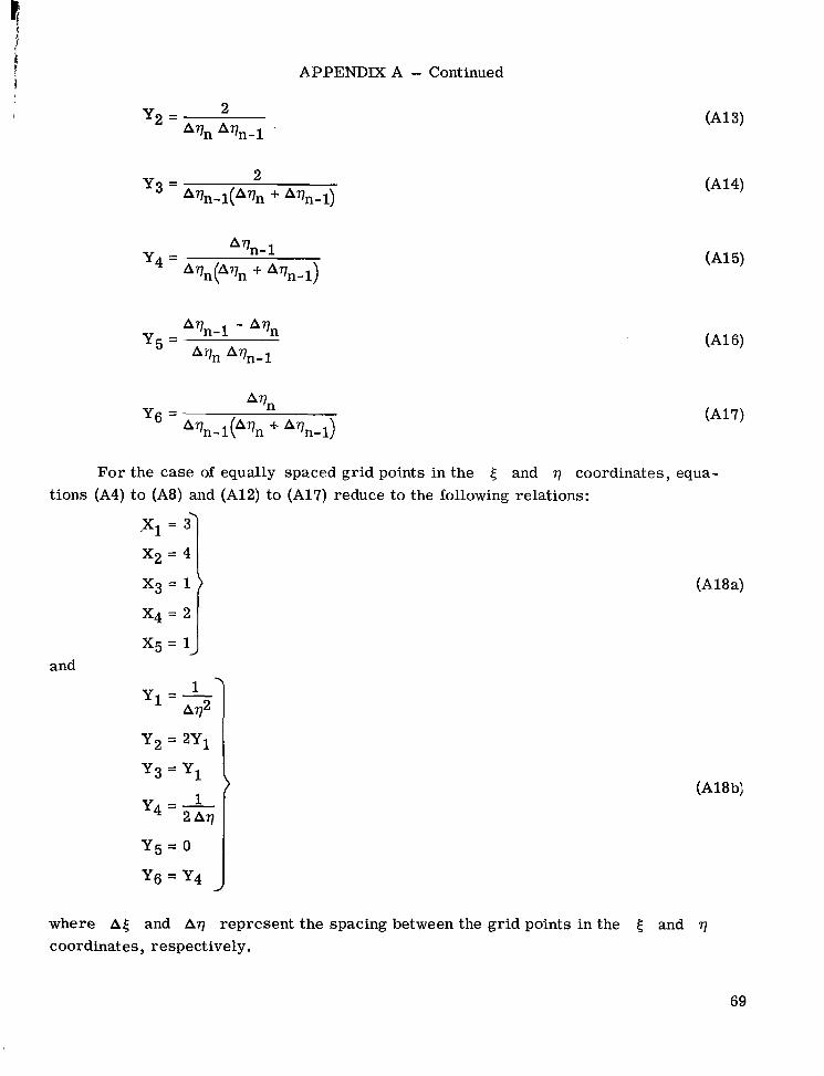
APPENDIX A - Continued

For the case of equally spaced grid points in the 5 and q coordinates, equations (A4) to (A8) and (A12) to (A17) reduce to the following relations: .

,XI = 3

x 2 = 4

x 3 = 1

x 4 = 2

x 5 = 1 I and

Y2 = 2Y1

Y3 = Y1

y4 = 1 2 All

Y5 = 0

(A18a)

(A18b)

where A( and Aq represent the spacing between the grid points in the C; and q coordinates, respectively.

69

APPENDMA - Continued

Equations (A2), (A3), (AlO), and (All) can then be written for constant grid-point spacing as follows:

Equations (A19) to (A22) a r e recognized as the standard relations for equally spaced grid points. (See, for example, ref. 30.)

Quantities of the form (G z) that appear in the governing equations must be

linearized in order to obtain a system of linear difference equations. Quantities of this type a re linearized by using equations (A2) and (A3); that is,

The procedure used

(A231

to linearize nonlinear products such as ( aG/ aq) ( aH/ av) is the same as that used by Flugge-Lotz and Blottner (ref. 29) and is as follows:

where the te rms and

known station m. By equating

quantities of the type (zr is a re evaluated from equation (A1 1) ,.but at the

G to--’H in equation (A24), the linearized form for

obtained; that is,

APPENDIXA - Concluded

m+l ,n

where ($) is obtained from equation (A22). m+l ,n

The preceding relations for the difference quotients produce linear difference equations (eqs. (66 ) and (67)) when substituted into the governing differential equations for the conservation of momentum (eq. (26)) and energy (eq. (27)), respectively, since te rms of order (A[)2 a r e neglected.

71

APPENDIX B

COEFFICIENTS FOR DIFFERENCE EQUATIONS

Equations (66) and (67) are the difference equations used to represent the partial differential equations for the conservation of momentum and energy, respectively. These

equations are repeated for convenience as follows:

These equations are obtained from equations (26) and (27) and the difference quotients presented in appendix A. The coefficients Ai'), BL'), and so forth, in equations (Bl) and (B2) are functions of known quantities evaluated at stations m and m - 1. (See fig. 7.) procedures. The coefficients a r e as follows:

Therefore, equations (Bl) and (B2) can be solved simultaneously without iterative

A(1) = Y3H3 - Y6Hll 033) n

G!) = H1Fm2 + H4TyFy 039)

72

APPENDIX B - Continued

F ( ~ ) n = Y ~ H ~ ~ + ~ 4 ~ 1 2

d2) n = H1Tm2 + H ~ ( F Y ) ~ + H ~ ( T Y ) ~

(B15)

(BIG)

The coefficients Y1,Y2, . . ., Y6, XI, . . ., X5, etc., a r e functions of the grid- point spacing and are defined in equations (A12) to (A17) and (A4) to (A8), respectively. The coefficients HI, H2, . . . are defined as follows:

(B17)

( B W

FT

2 '1 = $n+lFm1

~2 = v m 1 - L m l ( E m l c L l + C n 1 C m ~ )

73


HI1 = H2 + N4Ty

H12 = H7 + 2HgTy

0327)

(B28)

The undefined quantities appearing in equations (B17) to (B28) are defined as follows:

(E3291

(Air only) 0334)

(Air only) 0335)

(See eq. (74)) 0336)

74

I


'Y = Y4'm,n+l Y5'm,n - Y6'm,n-l

g)m+l (See eq. (28))

The transverse curvature t e rms a r e contained in the quantities Cml and CAI which appear explicitly in the H2, H3, H7, Hg, and H9 coefficients. The transverse curvature te rm in the transformed plane (see eq. (30)) may be written as follows:

where t represents the ratio r/ro and is a known quantity for the N - 1 grid points at station m - 1 and m. Then, the extrapolated values at m + 1, n a re obtained as follows where the parameter C is used to represent t : 2 j

Two quantities (symbols) as of now remain undefined. These a r e the code symbols FT and W which appear in equations (B17) and (B44), respectively. The code symbol W appearing in equation (B44) is used to either retain or neglect the transverse curvature t e rms for axisymmetric flows; that is, W = 1 o r 0, respectively. flows, the transverse curvature te rm does not appear since j equals 0. The code symbol FT (flow type) appearing in equation (B17) is used to either retain or neglect the nonsimilar t e rms in the governing differential equations; that is, tively. If FT is assigned a value of unity, the solution t o the nonsimilar equations

For planar

F T = 1 or 0, respec-

75

I

APPENDIX B - Concluded

(eqs. (25) to (27)) is obtained. If FT is assigned a value of zero, the locally similar solution is obtained; that is, the following system of equations are solved:

Continuity: av --+F=O arl

Momentum:

Energy:

The governing equations for the locally similar system a re obtained from equations (25) to (27) by neglecting derivatives of the dependent variables F, 0, and V with respect to the streamwise coordinate 5 . The capability of obtaining locally s imilar solutions is desirable in that for a given test case the locally similar and completely nonsimilar solutions can be obtained for the identical program inputs and numerical procedures. Consequently, the effects of the nonsimilar te rms on the boundary-layer characteristics for a particular case can be determined by direct comparison of the results obtained for solutions for FT = 1 and FT = 0, fespectively.

76

REFERENCES

1. Prandtl, L.: h e r FlGssigkeitsbewegung bei sehr kleiner Reibung. Verh. des III. Int. Math-Kong., Heidelberg, B. G. Teubner (Leipzig), 1904, pp. 484-491.

2. Schlichting, Hermann (J. Kestin, Transl.): Boundary-Layer Theory. Sixth ed., McGraw-Hill Book Co., 1968.

3. Moore, F. K., ed.: Hypersonic Boundary Layer Theory. Theory of Laminar Flows. Vol. IV of High Speed Aerodynamics and Je t Propulsion, F. K. Moore, ed., Princeton Univ. P res s , 1964, pp. 439-527.

4. Rosenhead, L., ed.: Laminar Boundary Layers. Clarendon P res s (Oxford), 1963.

5. Dewey, C. Forbes, Jr.; and Gross, Joseph F.: Exact Similar Solutions of the Laminar Boundary-Layer Equations. Rand Corp., July 1967.

Mem. RM-5089-ARPA (Contract No. DAH15 67 C 0141), (Available from DDC as AD 665 969.)

6. Blottner, F. G.: Finite Difference Methods of Solution of the Boundary-Layer Equa- tions. AIAA J., vol. 8, no. 2, Feb. 1970, pp. 193-205.

7. Tani, Itiro; and Hama, Francis R.: Some Experiments on the Effect of a Single Rough- ness Element on Boundary-Layer Transition. J. Aeronaut. Sci., vol. 20, no. 4, Apr. 1953, pp. 289-290.

8. Mitchner, Morton: Propagation of Turbulence From an Instantaneous Point Distur- bance. J. Aeronaut. Sci., vol. 21, no. 5, May 1954, pp. 350-351.

9. Schubauer, G. B.; and Klebanoff, P. S.: Contributions on the Mechanics of Boundary- Layer Transition. NACA Rep. 1289, 1956. (Supersedes NACA TN 3489.)

10. James, Carlton S.: Observations of Turbulent-Burst Geometry and Growth in Super- sonic Flow. NACA TN 4235, 1958.

11. S'ivulescu, St. N.: Tranzitia de la Scurgerea Laminara la Cea Turbulenta. Editura Academiei Republicii Socialiste Romgnia, 1968.

12. Morkovin, Mark V.: Critical Evaluation of Transition From Laminar t o Turbulent Shear Layers With Emphasis on Hypersonically Traveling Bodies. AFFDL-TR-68-149, U.S. Air Force, Mar. 1969. (Available from DDC as AD 686 178.)

13. Mack, Leslie M.; and Morkovin, Mark V.: High Speed Boundary-Layer Stability and Transition. AIAA Professional Study Series, 1969.

14. Kline, S. J.; Morkovin, M. V.; Sovran, G.; and Cockrell, D. J., eds.: Computation of Turbulent Boundary Layers - 1968 AFOSR-IFP-Stanford Conference. Vol. I - Methods, Predictions, Evaluation and Flow Structure. Stanford Univ., c.1969.

77

15. Coles, D. E.; and Hirst, E. A., eds.: Computation of Turbulent Boundary Layers - 1968 AFOSR-IFP-Stanford Conference. Vol. 11 - Compiled Data. Stanford Univ., c.1969.

16. Anon.: Compressible Turbulent Boundary Layers. NASA SP-216, 1969.

17. Beckwith, Ivan E.: Recent Advances in Research on Compressible Turbulent Bound- a ry Layers. Analytic Methods in Aircraft Aerodynamics, NASA SP-228, 1970, pp. 355-416.

18. Persh, Jerome: A Procedure for Calculating the Boundary-Layer Development in the Region of Transition From Laminar to Turbulent Flow. NAVORD Rep. 4438, U.S. Navy, Mar. 19, 1957. (Available from DDC as AD 131 947.)

19. Weber, H. E.: Turbulent and Transition Boundary Layer Based on Mixing Length and Intermittency. Paper 68-FE-52, Amer. SOC. Mech. Eng., May 1968.

20. Emmons, H. W.: The Laminar-Turbulent Transition in a Boundary Layer - Pt. I., J. Aeronaut. Sci., vol. 18, no. 7, July 1951, pp. 490-498.

21. Masaki, M.; and Yakura, J. K.: Transitional Boundary Layer Considerations for the Heating Analyses of Lifting Reentry Vehicles. AIAA Paper No. 68-1155, Dec. 1968.

22. Martellucci, A.; Rie, H.; and Sontowski, J. F.: Evaluation of Several Eddy Viscosity Models Through Comparison With Measurements in Hypersonic Flows. AIAA Paper No. 69-688, June 1969.

23. Harr is , Julius Elmore: Numerical Solution of the Compressible Laminar, Transi- tional, and Turbulent Boundary Layer Equations With Comparisons to Experimental Data. Ph. D. Thesis, Virginia Polytech. Inst., May 1970.

24. Adams, John C., Jr.: Eddy Viscosity-Intermittency Factor Approach to Numerical Calculation of Transitional Heating on Sharp Cones in Hypersonic Flow. AEDC-TR-70-210, U.S. Air Force, Nov. 1970.

25. Kuhn, Gary D.: Calculation of Compressible, Nonadiabatic Boundary Layers in Laminar, Transitional and Turbulent Flow by the Method of Integral Relations. NASA CR-1797, 1970.

26. Fish, R. W.; and McDonald, H.: Practical Calculations of Transitional Boundary Layers. Rep. UAR-H48, United Aircraft Corp., Mar. 14, 1969.

27. Glushko, G. S.: Turbulent Boundary Layer on a Flat Plate in an Incompressible Fluid. Bull. Acad. Sci. USSR, Mech. Ser., no. 4, 1965, pp. 13-23.

28. Donaldson, Coleman duP.; and Rosenbaum, Harold: Calculation of Turbulent Shear Flows Through Closure of the Reynolds Equations by Invariant Modeling. Rep. No. 127, Aeronaut. Res. Assoc. Princeton, Inc., Dec. 1968.

78

29. Fliigge-Lotz, I.; and Blottner, F. G.: Computation of the Compressible Laminar Boundary-Layer Flow ‘Including Displacement-Thickness Interaction Using Finite- Difference Methods. AFOSR 2206, U.S. Air Force, Jan. 1962.

30. Davis, R. T.; and Flzgge-Lotz, I.: Laminar Compressible Flow Past h i s y m m e t r i c Blunt Bodies (Results of a Second-Order Theory). Tech. Rep. No. 143 (Grants AF-AFOSR-62-242 and AF-AFOSR-235-63), Div. Eng. Mech., Stanford Univ., Dec. 1963.

31. Reynolds, Osborne: An Experimental Investigation of the Circumstances Which Determine Whether the Motion of Water in Parallel Channels Shall be Direct o r Sinuous and of the Law of Resistance in Parallel Channels. Phil. Trans. Roy. SOC. London, vol. 174, 1883, pp. 935-982.

32. Van Driest, E. R.: Turbulent Boundary Layer in Compressible Fluids. J. Aeronaut. Sci., vol. 18, no. 3, Mar. 1951, pp. 145-160, 216.

33. Bushnell, Dennis M.; and Beckwith, Ivan E.: Calculation of Nonequilibrium Hyper- sonic Turbulent Boundary Layers and Comparisons With Experimental Data. AIAA J., vol. 8, no. 8, Aug. 1970, pp. 1462-1469.

34. Probstein, Ronald F.; and Elliott, David: The Transverse Curvature Effect in Com- pressible Axially Symmetric Laminar Boundary-Layer Flow. J. Aeronaut. Sci., vol. 23, no. 3, Mar. 1956, pp. 208-224, 236.

35. Hayes, Wallace D.; and Probstein, Ronald F.: Hypersonic Flow Theory. Academic P res s , Inc., 1959.

36. Bradshaw, P.: Turbulent Boundary Layers. Aeronaut. J., vol. 72, no. 689, May 1968, pp. 451-458.

37. Prandtl, L.: Report on Investigation of Developed Turbulence. NACA TM 1231, 1949.

38. Van Driest, E. R.: On Turbulent Flow Near a Wall. J. Aeronaut. Sci., vol. 23, no. 11, NOV. 1956, pp. 1007-1011.

39. Stokes, G. G.: On the Effect of the Internal Friction of Fluids on the Motion of Pendulums. Trans. Cambridge Phil. SOC., vol. IX, pt. 11, 1851, pp. 8-106.

40. Bushnell, Dennis M.; and Morris, Dana J.: Shear Stress, Eddy Viscosity, and Mixing Length Distributions in Hypersonic Turbulent Boundary Layers. NASA TM X-2310, 1971.

41. Cebeci, Tuncer: Behavior of Turbulent Flow Near a Porous Wall With Pressure Gradient. AIAA J., vol. 8, no. 12, Dec. 1970, pp. 2152-2156.

79

42. Clauser, Francis H.: The Turbulent Boundary Layer. Vol. IV of Advances in Applied Mechanics, H. L. Dryden and Th. von K5rm%n, eds., Academic Press, Inc., 1956, pp. 1-51.

43. Maise, George; and McDonald, Henry: Mixing Length and Kinematic Eddy Viscosity in a Compressible Boundary Layer. AIAA J., vol. 6, no. 1, Jan. 1968, pp. 73-80.

44. Morkovin, Mark V.: Effects of Compressibility on Turbulent Flows, The Mechanics of Turbulence, Gordon & Breach, Sci. Publ., Inc., c.1964, pp. 367-380.

45. Matsui, Tatsuya: Mean Velocity Distribution in the Outer Layer of a Turbulent Boundary Layer. Res. Rep. No. 42 (Contract NONR 978(03)), Aerophys. Dep., Mississippi State Univ., Feb. 19, 1963.

46. Klebanoff, P. S.: Characteristics of Turbulence in a Boundary Layer With Zero Pressure Gradient. NACA Rep. 1247, 1955. (Supersedes NACA TN 3178.)

47. Kestin, J.; and Richardson, P. D.: Heat Transfer Across Turbulent Incompressible Boundary Layers. The Mechanics of Turbulence, Gordon & Breach, Sci. Publ., Inc., c.1964, pp. 409-418.

48. Johnson, Donald S.: Turbulent Heat Transfer in a Boundary Layer With Discon- tinuous Wall Temperature. Publ. No. 55 (OSR Tech. Note 55-289), Dep. Aeronaut., The Johns Hopkins Univ., Aug. 1955.

49. Rochelle, William C.: Prandtl Number Distribution in a Turbulent Boundary Layer With Heat Transfer at Supersonic Speeds. DRL-508 (Grants DA-ORD-31-124-61-G3 and DA-ORD(D)-31-124-G132), Univ. of Texas, Oct. 1963. (Available from DDC as AD 427 156.)

50. Simpson, R. L.; Whitten, D. G.; and Moffat, R. J.: An Experimental Study of the Turbulent Prandtl Number of Air With Injection and Suction. Int. J. Heat Mass Transfer, vol. 13, no, 1, Jan. 1970, pp. 125-143.

51. Rotta, J. C.: Heat Transfer and Temperature Distribution in Turbulent Boundary Layers at Supersonic and Hypersonic Flow. AGARDograph 97, Pt. I, May 1965, pp. 35-63.

52. Cebeci, Tuncer: A Model for Eddy-Conductivity and Turbulent Prandtl Number. Rep. No. MDC-J0747/01, McDonnell Douglas Corp., May 1970.

53. Jenkins, Rodman: Variation of the Eddy Conductivity With Prandtl Modulus and Its Use in Prediction of Turbulent Heat Transfer Coefficients. 1951 Heat Transfer and Fluid Mechanics Institute, Stanford Univ. Press, June 1951, pp. 147-158, 266-267.

54. Meier, H. U.; and Rotta, J. C.: Experimental and Theoretical Investigations of Tem- perature Distributions in Supersonic Boundary Layers. AIAA Paper No. 70-744, June-July 1970.

80

55. McDonald, H.: Mixing Length and Kinematic Eddy Viscosity in a Low Reynolds

1970.

I1

I Number Boundary Layer. Rep. J214453-1, Res. Lab., United Aircraft Corp., Sept.

56. Simpson, Roger Lyndon: The Turbulent Boundary Layer on a Porous Plate: An Experimental Study of the Fluid Dynamics With Injection and Suction. Ph. D. Thesis, Stanford Univ., 1968.

57. Whitten, Derril l Gene: The Turbulent Boundary .Layer on a Porous Plate: Experi- mental Heat Transfer With Variable Suction, Blowing and Surface Temperature. Ph. D. Thesis, Stanford Univ., 1968.

58. Lin, C. C.: On the Stability of Two-Dimensional Parallel Flows. Part I - General Theory. Quart. Appl. Math., vol. 111, no. 2, July 1945, pp. 117-142.

59. Lin, C. C.: The Theory of Hydrodynamic Stability. Cambridge Univ. Press, 1955.

60. Jaffe, N. A.; Okamura, T. T.; and Smith, A. M. 0.: Determination of Spatial Amplifi- cation Factors and Their Application to Predicting Transition. no. 2, Feb. 1970, pp. 301-308.

AIAA J., vol. 8,

61. Fischer, Michael Carlton: An Experimental Investigation on Unit Reynolds Number and Bluntness Effects on Boundary-Layer Transition for a 10' Half-Angle Cone at M, = 7. M.S. Thesis, Virginia Polytech. Inst., June 1969.

62. Pate, S. R.; and Schueler, C . J.: BP'fects of Radiated Aerodynamic Noise on Model Boundary-Layer Transition in Supersonic and Hypersonic Wind Tunnels. AEDC-TR-67-236, U.S. Air Force, Mar. 1968. (Available from DDC as AD 666 644.)

63. Softley, E. J.; Graber, B. C.; and Zempel, R. E.: Transition of the Hypersonic Boundary Layer on a Cone: Pt. I - Experiments at M, = 12 and 15. R67SD39 (Contract A F 04(694)-772), Missile Space Div., Gen. Elec. Co., Nov. 1967. (Avail- able from DDC as AD 824 681.)

64. Richards, Bryan E.: Transitional and Turbulent Boundary Layers on a Cold Flat Plate in Hypersonic Flow. Aeronaut. Quart., vol. XVIII, Pt. 3, Aug. 1967, pp. 237-257.

65. Potter, J. Leith; and Whitfield, Jack D.: sonic Conditions. Recent Development in Boundary Layer Research, Pt. 111, AGARDograph 97, May 1965, pp. 1-62.

66. Deem, Ralph E.; and Murphy, James S.: Flat Plate Boundary Layer Transition at

Boundary-Layer Transition Under Hyper-

Hypersonic Speeds. AIAA Paper No. 65-128, Jan. 1965.

81

1lI111111111111l I 1111

67. Cary, Aubrey M,, Jr.: Turbulent Boundary Layer Heat Transfer and Transition Measurements With Extreme Surface Cooling in Hypersonic Flow. M.A.E. Thesis, Univ. of Virginia, Aug. 1969.

68. Potter, J. Leith; and Whitfield, Jack D.: Effects of Slight Nose Bluntness and Rough- ness on Boundary-Layer Transition in Supersonic Flows. J. Fluid Mech., vol. 12, pt. 4, Apr. 1962, pp. 501-535.

69. Rouse, Hunter: A General Stability Index for Flow Near Plane Boundaries. J. Aeronaut. Sci., vol. 12, no. 4, Oct. 1945, pp. 429-431.

70. Van Driest , E. R.; and Blumer, C. B.: Boundary Layer Transition: Freestream Turbulence and Pressure Gradient Effects. AIAA J., vol. 1, no. 6, June 1963, pp. 1303-1306.

71. Ivensen, H. W.; and Hsu, Tao-Ting: A Local Reynolds Number to Predict Transition From Laminar to Turbulent Flow. Heat Transfer Thermodynamics and Education, Harold A. Johnson, ed., McGraw-Hill Book Co., Inc., 1964, pp. 207-212.

72. Stainback, P. Calvin: Use of Rouse's Stability Parameter in Determining the Critical Layer Height of a Laminar Boundary Layer. AIAA J., vol. 8, no. 1, Jan. 1970, pp. 173-175.

73. McCauley, William D., ed.: Boundary Layer Transition Study Group Meeting. Vol. 111 - Session on Ground Test Transition Data and Correlations. BSD-TR-67-213, Vol. 111, U.S. Air Force, Aug. 1967.

74. McCauley, William D., ed.: Boundary Layer Transition Study Group Meeting. Vol. I - Session on Flight Test Transition Data and Correlations. Vol. I, U.S. Air Force, Aug. 1967.

BSD-TR-67-213,

75. McCauley, William D., ed.: Boundary Layer Transition Study Group Meeting. Vol. I1 - Session on Boundary Layer Stability. BSD-TR-67-213, Vol. 11, U S . Air Force, Aug. 1967. (Available from DDC as AD 820 364.)

76. McCauley, William D., ed.: Boundary Layer Transition Study Group Meeting. BSD-TR-67-213, Vol. IV - Session on Boundary Layer Transition Control.

Vol. IVY U S . Air Force, Aug. 1967.

.77. Dhawan, S.; and Narasimha, R.: Some Properties of Boundary Layer Flow During the Transition From Laminar to Turbulent Motion. J. Fluid Mech., vol; 3, pt. 4, Jan. 1958, pp. 418-436.

78. Corrsin, Stanley; and Kistler, Alan L.: Free-Stream Boundaries of Turbulent Flows. NACA Rep. 1244, 1955. (Supersedes NACA TN 3133.)

82

I

79. Fiedler, H.: Intermittency Distributions in Turbulent Wall Boundary Layers With and Without P res su re Gradients. NASA TT F-11,326, 1967.

80. Young, C. H.; Reda, D. C.; and Roberge, A. M.: Hypersonic Transitional and Turbu- lent Flow Studies on a Lifting Entry Vehicle. AIAA Paper No. 71-100, Jan. 1971.

1 1 'i I

81. Smith, A. M. 0.; and Cebeci, T.: Numerical Solution of the Turbulent-Boundary- Layer Equations. Rep. No. DAC 33735 (Contract NOW 66-0324-c), Douglas Aircraft Co., Inc., May 29, 1967.

I

82. Keller, Herbert B.; and Cebeci, Tuncer: Accurate Numerical Methods for Boundary Layer Flows. 11. Two-Dimensional Turbulent Flows. AIM Paper No. 71-164, Jan. 1971.

83. Cebeci, Tuncer; Smith, A. M. 0.; and Mosinkis, G.: Calculation of Compressible Adiabatic Turbulent Boundary Layers. AIAA Paper No. 69-687, June 1969.

84. Beckwith, Ivan E.; and Bushnell, Dennis M. (With appendix C by Carolyn C. Thomas): Detailed Description and Results of a Method fo r Computing Mean and Fluctuating Quantities in Turbulent Boundary Layers. NASA TN D-4815, 1968.

85. McLafferty, George H.; and Barber, Robert E.: Turbulent Boundary Layer Charac- teristics in Supersonic Streams Having Adverse Pressure Gradients. Rep. R-1285-11 (Contract No. NOa(s) 55-133-c), Res. Dep., United Aircraft Corp., Sept. 1959.

86. Moore, D. R.; and Harkness, J.: Experimental Investigation of the Compressible Turbulent Boundary Layer at Very High Reynolds Numbers, M = 2.8. Rep. No. 0-71000/4R-9, LTV Res. Center, Apr. 1964.

87. Coles, Donald: Measurements in the Boundary Layer on a Smooth Flat Plate in Supersonic Flow. Jet Propulsion Lab., California Inst. Technol. 111. Measure- ments in a Flat-Plate Boundary Layer at the Jet Propulsion Laboratory. No. 20-71 (Contract No. DA-04-495-0rd 18), June 1, 1953.

Rep.

88. Marvin, Joseph G.; and Akin, Clifford M.: Combined Effects of Mass Addition and Nose Bluntness of Boundary-Layer Transition. AIAA Paper No. 69-706, June 1969,

89. Marvin, Joseph G.; and Sheaffer, Yvonne S.: A Method for Solving the Nonsimilar Laminar Boundary-Layer Equations Including Foreign Gas Injection. NASA TN D-5516, 1969.

90. Clutter, Darwin W.; and Smith, A. M. 0.: Solution of the General Boundary-Layer Equations for Compressible Laminar Flow, Including Transverse Curvature. Rep. No. L B 31088 (Contract NOW 60-0553c), Douglas Aircraft Co., Inc., Feb. 15, 1963.

83

91. Bushnell, Dennis M.; Jones, Robert A.; and Huffman, Jarrett K.: Heat-Transfer and Pressure Distributions on Spherically Blunted 25' Half-Angle Cone at Mach 8 and Angles of Attack up t o 90°. NASA TN D-4792, 1968.

92. Lomax, Harvard; and Inouye, Mamoru: Numerical Analysis of Flow Properties About Blunt Bodies Moving at Supersonic Speeds in an Equilibrium Gas. NASA TR R-204, 1964.

93. Winter, K. G.; Rotta, J. C.; and Smith, K. G.: Untersuchungen der turbulenten Grenzschicht an einem taillierten Drehkcrper bel Unter- und Uberschallstr6mung, DLR FR 65-52, NOV. 1965.

94. Herring, H. James; and Mellor, George L.: A Method of Calculating Compressible Turbulent Boundary Layers. NASA CR-1144, 1968.

95. Sims, Joseph L.: Tables for Supersonic Flow Around Right Circular Cones at Zero Angle of Attack. NASA SP-3004, 1964.

96. O'Donnell, Robert M.: Experimental Investigation at a Mach Number of 2.41 of Average Skin- Friction Coefficients and Velocity Profiles for Laminar and Turbu- lent Boundary Layers and an Assessment of Probe Effects. NACA TN 3122, 1954.

97. Johnson, Charles B.: Pressure and Flow-Field Study at Mach Number 8 of Flow Separation on a Flat Plate With Deflected Trailing-Edge Flap. NASA TN D-4308, 1968.

84 NASA-Langley, 1971 - 12 L-7660

NATIONAL AERONAUTICS AND SPACE ADMINISTRA? ION

WASHINGTON, D. C. 20546

0 2 1 0 0 1 c 1 IT 1 2 7 1 0 8 1 3 sOC130qns DEPT OF THE 4 T R FORCE AF SYSTEMS C O Y Y A N D AF WEAPONS L A B (WLOL) ATTN: F: L O U B O W M A N , CFITRP TFCH LTl33DARY K T R T L A N D AFB NM 97117

OFFICIAL BUSINESS PENALTY FOR PRIVATE USE $300

Jl

/-

c

FIRST CLASS MAIL

POSTAGE AND FEES PAID NATIONAL AERONAUTICS AND

SPACE ADMINISTRATION

‘ T h e aeronautical and space activities of the United States shall be condwted s o a s t o contribute . . . to the expansioit of himan knowledge of phenoniena in the atniosphere and *ace. T h e Administration shall provide f o r the widest prncticable and appropriate dissemination of information concerning its actiqities and the res& thereof.”

, -NATIONAL AERONAUTICS AND SPACE ACT OF 1958

NASA SCIENTIFIC AND TECHNICAL -PUBLICATIONS >

TECHNICAL REPORTS: Scientific and technical information considered important, complete, and a lasting contribution to existi& knowledge.

TECHNICAL YOTES: Information less broad in scope but nevertheless of importance as a contribution to existing knowledge.

TECHNICAL MEMORANDUMS:

because of preliminary data, security classifica- tion, or other reasons.

. Information receiving limited distribution

TECHNICAL TRANSLATIONS: Information published in a foreign language considered to merit NASA distribution in English.

SPECIAL PUBLICATIONS: Information derived from or of value to NASA activities. Publications include conference proceedings, monographs, data compilations, handbooks, sourcebooks, and special bibliographies.

TECHNOLOGY UTILIZATION PUBLICATIONS: Information on technology used by NASA that may be of particular interest in commercial and other non-aerospace applications. Publications include Tech Briefs, Technology Utilization Reports and Technology Surveys.

‘ CONTRACTOR REPORTS: Scientific and technical information generated under a NASA contract or grant and considered an important contribution to existing knowledge.

Details on the availability of ihese publications may be obtained from:

SCIENTIFIC AND TECHNICAL INFORMATION OFFICE

NATlO NA L AER 0 N AUT1 C S AN D SPACE ADM I N I STRATI 0 N Washington, D.C. 20546

TECHNICAL --- NASA REPORT

Documents

Transcript of TECHNICAL --- NASA REPORT