Technical Improvements in Quantitative Susceptibility Mapping · PDF fileTECHNICAL...
214
TECHNICAL IMPROVEMENTS IN QUANTITATIVE SUSCEPTIBILITY MAPPING
-
Upload
nguyenquynh -
Category
Documents
-
view
224 -
download
0
Transcript of Technical Improvements in Quantitative Susceptibility Mapping · PDF fileTECHNICAL...

TECHNICAL IMPROVEMENTS IN
QUANTITATIVE SUSCEPTIBILITY MAPPING


TECHNICAL IMPROVEMENTS IN
QUANTITATIVE SUSCEPTIBILITY MAPPING
BY
SAIFENG LIU B.Sc.
A Thesis
Submitted to the School of Biomedical Engineering
and the School of Graduate Studies
of McMaster University
in Partial Fulfilment of the Requirements
for the Degree of
Doctor of Philosophy
© Copyright by Saifeng Liu, April 2014
All Rights Reserved

ii
Ph. D. (2014) McMaster University
(School of Biomedical Engineering) Hamilton, Ontario, Canada
TITLE: Technical Improvements in Quantitative Susceptibility Mapping
AUTHOR: Saifeng Liu
B.Sc., (Biomedical Engineering)
Huazhong University of Science and Technology
Wuhan, China
SUPERVISOR: E. Mark Haacke Ph. D.
NUMBER OF PAGES: xx, 192

iii
To my parents
Fenling Liu and Yongqi Liu

iv
Abstract
Quantitative susceptibility mapping (QSM) is a promising technique to study tissue
properties and function in vivo. The presence of a susceptibility source will lead to a non-
local field variation which manifests as a non-local behavior in magnetic resonance phase
images. QSM is an ill-posed inverse problem that maps the phase back to the
susceptibility source. In practice, the phase images are usually contaminated by
background field inhomogeneities. Consequently, the efficacy and accuracy of QSM rely
on background field removal. In this thesis, several technical advances in QSM have been
made which accelerate the data processing and improve the accuracy of this ill-posed
problem.
Different background field removal algorithms are analyzed and compared in detail,
including homodyne high-pass filtering, variable high-pass filtering, sophisticated
harmonic artefact reduction for phase data (SHARP), and projection onto the dipole field
(PDF). In these algorithms, phase unwrapping is usually required, which can be time-
consuming and sensitive to noise. To solve this problem, a new background field removal
algorithm, local spherical mean value filtering (LSMV), is proposed, in which the global
phase unwrapping is bypassed. This algorithm improves the time-efficiency and
robustness of background field removal, especially for double-echo data.
The simplest algorithm to solve the inverse problem is the regularization process using
truncated k-space division. However, this algorithm induces streaking artefacts in the
v
susceptibility maps. The streaking artefacts can be reduced dramatically using geometry
constraints. In the k-space/image domain iterative algorithm for susceptibility weighted
imaging and mapping (SWIM), the geometries extracted from the initial susceptibility
maps are used to update the data in the singularity regions in k-space. An improved
version of this algorithm is demonstrated using multi-level thresholding to account for the
variation in the susceptibilities of different structures in the brain.
These susceptibility maps could be used to generate orientation independent weighting
masks, to form a new type of susceptibility weighted image (SWI), referred to here as
true-SWI (tSWI). The tSWI data show improved contrast-to-noise ratio (CNR) of the
veins and reduced blooming artefacts due to the strong dipolar phase of microbleeds.
Finally, the accuracy in estimating the susceptibility of a small object is usually hampered
by partial volume effects. In this thesis, it is shown that the effective magnetic moment,
being the product of the apparent volume and the measured susceptibility of the small
object, is constant and can be used to improve the susceptibility quantification, if a priori
information of the volume is available.
In conclusion, the technical improvements presented in this thesis contribute to a better
data processing scheme for QSM, with accelerated data processing by using the LSMV
algorithm for background field removal, reduced streaking artefacts in the susceptibility
maps by using the iterative SWIM algorithm for solving the inverse problem, and
improved accuracy by proper handling of the partial volume effects using volume
constraints.

vi
Acknowledgements
I would like to express my deepest appreciation to my supervisor, Dr. E. Mark Haacke,
for his enduring support and persistent inspiration. It is Dr. Haacke who led me into the
exciting and intriguing world of MRI. As one of the great scientists in this field,
Dr. Haacke has demonstrated to me how the knowledge of spins in MRI and expertise in
physics can be applied to both MRI and tennis. It is his passion for both research and life
that has encouraged me to finish the work presented in this thesis.
I would like to thank my supervisory committee members, Dr. Nicholas Bock,
Dr. Qiyin Fang, and Dr. Maureen MacDonald, for their valuable guidance and comments.
Thanks to Dr. Michael Noseworthy, for helping me on extending my research horizon
and improving my teaching skills.
Moreover, I would like to thank Dr. Yu-Chung Norman Cheng, Dr. Yongquan Ye and
Dr. Jaladhar Neelavalli, for their careful reviewing of my thesis. Thanks to my colleagues
and friends Sagar Buch M. Sc., Jin Tang Ph.D., Eyesha Hashim, B. Sc., Weili Zheng
Ph.D. and Manju Liu M. Sc.
Finally, I wish to thank my grandfather Bingyan Liu (1933-2012) and grandmother
Hongzhu Liu, for their endless love.

vii
Contents
Abstract .............................................................................................................................. iv
Acknowledgements ........................................................................................................... vi
List of Figures .................................................................................................................... ix
List of Tables ................................................................................................................. xvii
List of Abbreviations ................................................................................................... xviii
1 Introduction ..................................................................................................................... 1
1.1 Background and significance ..................................................................................... 1
1.2 Review of QSM techniques ....................................................................................... 4
1.3 Overview of the thesis ............................................................................................... 7
2 Basic Concepts of Phase, Gradient Echo Imaging and Quantitative Susceptibility
Mapping ............................................................................................................................ 13
2.1 The concept of a gradient echo and phase ............................................................... 13
2.2 Predicting field variation through forward calculation ............................................ 20
2.3 Quantifying Susceptibility as an inverse problem ................................................... 23
2.4 Susceptibility and its relations to venous oxygen saturation and iron content ........ 25
3 Background Field Removal .......................................................................................... 29
3.1 The background field ............................................................................................... 29
3.2 Homodyne high-pass filter ....................................................................................... 31
3.3 Variable high-pass filter (VHP) ............................................................................... 37
3.4 Sophisticated Harmonic Artefact Reduction for Phase data (SHARP) ................... 44
3.5 Comparison of different background field removal algorithms............................... 49
4 Fast and Robust Background Field Removal using Double-echo Data ................... 62
4.1 Introduction .............................................................................................................. 62

viii
4.2 Theory ...................................................................................................................... 64
4.3 Materials and Methods ............................................................................................. 67
4.4 Results ...................................................................................................................... 74
4.5 Discussion ................................................................................................................ 85
5 Solving the Inverse Problem of Susceptibility Quantification .................................. 93
5.1 Susceptibility mapping using truncated k-space division ........................................ 93
5.2 Geometry constrained iterative reconstruction ...................................................... 100
5.3 Noise in susceptibility mapping ............................................................................. 120
5.4 Discussion and Conclusions .................................................................................. 124
6 Improved Venography using True Susceptibility Weighted Imaging (tSWI) ...... 129
6.1 Introduction ............................................................................................................ 129
6.2 Materials and Methods ........................................................................................... 131
6.3 Results .................................................................................................................... 139
6.4 Discussion .............................................................................................................. 150
7 Quantitative Susceptibility Mapping of Small Objects using Volume Constraints
.......................................................................................................................................... 157
7.1 Introduction ............................................................................................................ 157
7.2 Theory and Methods .............................................................................................. 159
7.3 Results .................................................................................................................... 169
7.4 Discussion and Conclusions .................................................................................. 177
8 Conclusions and Future Directions ........................................................................... 185

ix
List of Figures
Figure 2.1 Sequence diagram of a single echo 3D gradient echo sequence. GS: slab
selection/partition encoding gradient; GP: phase encoding gradient; GR: readout gradient.
............................................................................................................................................ 16
Figure 2.2 Illustration of filling one line in k-space. The k-space trajectory as indicated
by the dashed arrows is described using Eqs.2.8 to 2.10. .................................................. 17
Figure 2.3 Sequence diagram of a single echo 3D gradient echo sequence with flow-
compensation in all directions. GS: slab selection/partition encoding gradient; GP: phase
encoding gradient; GR: readout gradient. ........................................................................... 19
Figure 2.4 QSM data processing procedures. The dashed line indicates that brain masks
may not be required for phase unwrapping. The * indicates that the phase unwrapping
step can be avoided in certain algorithms and the unwrapped phase is not required for
background field removal. ................................................................................................. 23
Figure 3.1 Illustration of the processing steps in homodyne high-pass filtering. ............. 33
Figure 3.2 Relative error in estimated susceptibilities induced by high-pass filtering in
different orientations. The relative errors induced by homodyne high-pass filtering with
different sizes, for cylinders in the 90o case, are shown in a. b to e show the effects of the
orientation of high-pass filtering for cylinders in the 90o case (b), in the 30
o case (c), in
the 45o case (d), and in the 60
o case (e). Relative errors for the spheres are shown in f. .. 36
Figure 3.3 a). Simulated phase image with background phase but without random noise.
b). Simulated phase with background phase and random noise. c). The local phase
information without random noise. This is used as the true answer to evaluate the
accuracies of the processed phase images. d). The reference region used for calculating
the RMSEs in the processed phase images. e). The susceptibility map in axial view. f).
The phase image corresponds to e. .................................................................................... 40
Figure 3.4 Overall RMSEs of the processed phase images (a) and susceptibility maps (b)
generated using VHP. ........................................................................................................ 42
Figure 3.5 Relative errors in the estimated susceptibilities of different structures using
phase images processed by VHP. a) Veins. b) Globus pallidus. c) Putamen. d) Caudate.
x
The dashed lines indicate the errors in estimated susceptibilities for different structures
using the phase images with ideal background field removal. .......................................... 43
Figure 3.6 a) Overall RMSEs for different radii of the spherical kernel and different
values of th in SHARP. b) Overall RMSE in susceptibility quantification for different
kernel sizes and different thresholds in SHARP. ............................................................... 46
Figure 3.7 Relative errors in measured susceptibilities using different parameters in
SHARP for different structures. ......................................................................................... 47
Figure 3.8 The minimal RMSEs for different structures at different radii of the spherical
kernel in SHARP. ............................................................................................................... 48
Figure 3.9 Susceptibility estimated using the original phase vs. the susceptibility
estimated using different phase processing methods: a) Homodyne HP32×32, b)
Homodyne HP64×64, c) SHARP (radius=8px, th=0.02), d) SHARP (radius=8px,
th=0.05), e) Variable HP, and f) PDF. ............................................................................... 54
Figure 3.10 Phase images processed with different algorithms in Dataset 1. a and e.
64x64 Homodyne high-pass filter. b and f: VHP. c and g: SHARP. d and h: PDF. ......... 56
Figure 3.11 Susceptibility maps generated with different algorithms in Dataset 1. a and e.
64×64 Homodyne high-pass filter. b and f: VHP. c and g: SHARP. d and h: PDF. ......... 56
Figure 3.12 The means and standard deviations of the measured susceptibility values for
different structures in different in vivo datasets. The error bars represent the standard
deviations of the measured susceptibilities in different datasets. GP: globus pallidus, PUT:
putamen, CN: caudate nucleus, SN: substantia nigra, RN: red nucleus, and THA:
thalamus. The asterisks indicate Tukey’s HSD significance: * p<0.05, ** p<0.01, ***
p<0.001. ............................................................................................................................. 57
Figure 4.1 Processing steps in LSMV for single echo phase data with short TE. ............ 72
Figure 4.2 RMSEs of the processed phase images (a and b) and the susceptibility maps (c
and d) at different noise levels for the simulated 3D brain model. The RMSEs in a and c
were calculated using all the pixels inside the brain, while the RMSEs in b and d were
calculated using only the pixels close to (or inside) the veins. The SNR represents the
signal-to-noise ratio in the magnitude images. .................................................................. 75
Figure 4.3 A comparison of the processing times using different algorithms at different
noise levels. ........................................................................................................................ 76
Figure 4.4 RMSEs in the processed phase images (a and b) and susceptibility maps (c
and d) of the cylinders at two TEs. The SNR represents the signal-to-noise ratio in the
magnitude images. ............................................................................................................. 77

xi
Figure 4.5 The original phase images and the local phase images generated using
different algorithms for the simulated cylinder at SNR=5:1 and SNR=20:1. The SNR
represents the signal-to-noise ratio in the magnitude images. The images in the second to
fourth columns are the central 64×64 pixels in the processed local phase images, as
indicated by the white dashed box in the top-left image. The errors in the local phase
images obtained using 3DSRNCP and Laplacian phase unwrapping are indicated by the
black arrows. ...................................................................................................................... 78
Figure 4.6 The original and processed phase images for Dataset 1. a) Original phase
image at TE1=7.38ms. b) Complex divided phase image with effective TE=2.84ms. c)
Original phase images at TE2=17.6ms. d) SMV filtered result (φSMV) at TE1. e) SMV
filtered result at ΔTE. f) SMV filtered result at TE2, calculated using the images shown in
e and d as e+2×d. g) Local phase image at TE1. h) Local phase image at ΔTE. i) local
phase image at TE2. ............................................................................................................ 79
Figure 4.7 Comparison between the local phase images and susceptibility maps generated
using LSMV (a, d and g) and those generated using 3DSRNCP (b, e and h) for Dataset 1.
The difference images are shown in c, f and i. The phase images in the first row are at
TE1, and the phase images in the second row are at TE2. The images in the third row are
susceptibility maps (SM) obtained using the phase images at TE2 (d and e). The scale bars
are for the difference images c, f and i only. Note the improvement in the SM using
LSMV thanks to the better recovery of phase around the veins. ....................................... 80
Figure 4.8 Comparison between the local phase images and susceptibility maps generated
using LSMV (a, d and g), and those generated using Laplacian phase unwrapping (b, e
and h) for Dataset 1. The difference images are shown in c, f and i. The phase images in
the first row are at TE1, and the phase images in the second row are at TE2. The images in
the third row are susceptibility maps obtained using the phase images at TE2 (d and e).
The scale bars are for the difference images c, f and i only. .............................................. 81
Figure 4.9 a) Original phase image at TE2 from Dataset 2 with cusp artefact. Note that,
this image was obtained using the built-in multi-channel data combination algorithm on
the scanner. b) Unwrapped phase image using 3DSRNCP. c) Unwrapped phase image
using Laplacian phase unwrapping. d) Local phase image generated using LSMV. e)
Local phase image generated using the unwrapped phase image shown in b. f) Local
phase image obtained using the unwrapped phase image shown in c. Cusp artefact caused
errors in the processed phase images, as indicated by the white arrows. .......................... 84
Figure 5.1 The cross-sections of (a and b) and (c and d). In a and c, the
cross-sections are parallel to the main field direction, in b and d, the cross-sections are
perpendicular to the main field direction. The white regions in a and b correspond to the

xii
regions where . The black dashed lines in a and c indicate the positions of
the cross-sections shown in b and d................................................................................... 94
Figure 5.2 The underestimation in the susceptibility values measured inside the cylinders
with different radii (a, c and e) and the standard deviations (b, d and f). a and b were
generated when no noise was added. For c and d, SNR=10:1 in the magnitude images;
while for e and f, SNR=5:1. ............................................................................................... 98
Figure 5.3 The mean susceptibility values (a, c and e) and the standard deviations (b, d
and f) measured in the background regions outside the cylinders. a and b were generated
when no noise was added. For c and d, SNR=10:1 in the magnitude images; while for e
and f, SNR=5:1. ................................................................................................................. 99
Figure 5.4 The cost function R(th) for different cylinders. R(th) was calculated using Eq.
5.7. The optimal th was determined as when R(th) was minimized. Particularly, when
SNR=10:1, the optimal ths were 0.12 (r=2px), 0.13(r=4px), 0.14 (r=8px), and 0.14
(r=16px). When SNR=5:1, the optimal ths were 0.1 (r=2px), 0.13(r=4px), 0.13 (r=8px),
and 0.14 (r=16px). ............................................................................................................ 100
Figure 5.5 Illustration of the processing steps of Iterative SWIM algorithm. ................ 103
Figure 5.6 The effects of the parameter th on the accuracies of the estimated
susceptibilities of different structures. a) The relative errors (absolute values) in the
measured mean susceptibilities at different values of th. b) The standard deviations of the
measured susceptibilities at different values of th. .......................................................... 106
Figure 5.7 Means and standard deviations of the susceptibility values of different
structures in the 3D brain model at different iteration steps. a and b: the mean
susceptibility values measured at different iteration steps. c to f: the standard deviations
measured at different iteration steps. The images in the first column (a, c and e) show the
changes in mean and standard deviation when a high χth was used in geometry extraction,
while the images in the second column show the results when a low χth was used in
geometry extraction. ........................................................................................................ 107
Figure 5.8 a) The initial susceptibility map. b) The final susceptibility map after iterative
SWIM. c) The difference between a and the ideal susceptibility map. d) The difference
between b and the ideal susceptibility map. .................................................................... 108
Figure 5.9 K-space profiles of the initial susceptibility map (a) and the final susceptibility
map after iterative SWIM algorithm (b). The errors in the k-space profiles in a and b are
shown in c and d, respectively. Specifically, the errors were calculated by comparing the
k-space of the generated susceptibility maps with the kspace of the ideal susceptibility
maps. Compared with the initial susceptibility maps, the final susceptibility maps after

xiii
iterative SWIM algorithm have reduced errors in the cone of singularities in k-space, as
indicated by the white arrows. ......................................................................................... 109
Figure 5.10 The extracted geometries of veins and grey matter structures (a and b) and
the susceptibility maps (c and d) for the in vivo data. a) Maximum intensity projection of
the binary masks of veins extracted using a high χth. b) One slice of the binary masks of
the grey matter structures extracted using a low χth. c) Maximum intensity projection of
the initial susceptibility maps. d) The corresponding susceptibility map to the binary
mask shown in b. ............................................................................................................. 110
Figure 5.11 Mean susceptibility values of veins and globus pallidus at different iteration
steps in the in vivo data. The figures in the first column were obtained when high χth was
used to extract the geometries of veins only, while the figures in the second column were
measured when low χth was used to extract the geometries of veins and other structures.
.......................................................................................................................................... 112
Figure 5.12 Mean susceptibility values of red nucleus (RN), caudate nucleus (CN) and
putamen (PUT) at different iteration steps in the in vivo data. The figures in the first
column were obtained when high χth was used to extract the geometries of veins only,
while the figures in the second column were measured when low χth was used to extract
the geometries of veins and other structures. ................................................................... 113
Figure 5.13 Standard deviations of the susceptibility values at different iteration steps for
different structures in the in vivo data. The figures in the first column were obtained when
high χth was used to extract the geometries of veins only, while the figures in the second
column were measured when low χth was used to extract the geometries of veins and other
structures. ......................................................................................................................... 114
Figure 5.14 Comparison between the initial susceptibiltiy maps (a and d) and the final
susceptibility maps (b and e). Their differences are shown in c and f (generated as b-a
and e-d). ........................................................................................................................... 115
Figure 5.15 The effects of the regularization parameter λ in MEDI. The average gradient
was measured in the low gradient regions in the converged susceptibility maps. ........... 116
Figure 5.16 Susceptibility maps generated using different values of regularization
parameter λ with MEDI. a and d: λ=10. b and e: λ=100. a and d: λ=1000. ................... 116
Figure 5.17 Comparison of susceptibility maps generated by iterative SWIM (a) and
MEDI (b). The profiles of the solid black lines across the vein of Galen in a and b are
shown in c. The profiles of the dashed black line in the cortical region were shown in d.
The corresponding magnitude image is shown in e, which does not have clear edge
information of the veins in the region indicated by the white arrow. .............................. 117

xiv
Figure 5.18 Distributions of the susceptibility values of the pixels inside the veins (a and
b) and inside the globus pallidus (c and d), measured from iterative SWIM generated
susceptibility maps (a and c) and from MEDI generated susceptibility maps (b and d). 118
Figure 5.19 The k-space profiles obtained using truncated k-space division (a), iterative
SWIM (b) and MEDI (c). The difference between b and c is shown in d. The window
levels in a, b, and c are the same. The major differences are seen along the cone of
singularities in k-space, as indicated by the white arrow. ................................................ 120
Figure 5.20 a) Standard deviation of susceptibilities measured in the background
reference region for cylinders with different radii. b) Standard deviation measured inside
the cylinders. c) Noise amplification factor α as a function of SNR in magnitude images,
when th=0.1. d) Noise amplification factor α as a function of relative errors in the
estimated susceptibilities, when SNR=10:1. The arrow shows the case when th=0.13,
α=3.3 and the underestimation of the susceptibility is 11.3%. ........................................ 123
Figure 6.1 A comparison between tSWI and SWI data processing steps. ...................... 132
Figure 6.2 Phase images (a and b), susceptibility maps (c and d) and tSWI images (e, f, g
and h) for simulated cylinders with and without homodyne high-pass filtering. Images in
the first and third columns are generated using the original phase images without high-
pass filtering, while images in the second and fourth columns are generated using high-
pass filtering. The tSWI images e and f were generated using χ1=0, χ2=0.45ppm, n=2;
while g and h were generated using χ1=3σχ, χ2=0.45ppm, n=4. σχ is the standard deviation
of a reference region measured from the susceptibility maps shown in c and d
(σχ=0.05ppm for both c and d). The SNR in the original magnitude image was set to be
10:1 and the CNR between the cylinders and background in the original magnitude
images was basically zero. ............................................................................................... 140
Figure 6.3 Measured CNRs of cylinders from simulated tSWI images. Figures in
different rows were generated using different χ2 values, while figures in different columns
were generated using different χ1 values. a) χ1=0, χ2=1ppm; b) χ1=3σχ, χ2=1ppm; c) χ1=0,
χ2=0.45ppm; d) χ1=3σχ, χ2=0.45ppm; e) χ1=0, χ2=0.45ppm; and f) χ1=3σχ, χ2=0.45ppm.
To evaluate the effect of high-pass filtering, e and f were generated using high-pass
filtered phase images. ....................................................................................................... 141
Figure 6.4 Theoretically predicted CNRs of cylinders with different susceptibility values.
Figures in different rows were generated using different χ2 values, while figures in
different columns were generated using different χ1 values. a) χ1=0, χ2=1ppm; b) χ1=3σχ,
χ2=1ppm; c) χ1=0, χ2=0.45ppm; and d) χ1=3σχ, χ2=0.45ppm. ......................................... 142
Figure 6.5 Local CNRs of the right septal vein (a, c, and e) and the left internal cerebral
vein (b, d, and f) from different datasets with isotropic resolution. a, b, c and d were

xv
generated when threshold χ1=0 was used to create the susceptibility weighting masks,
while e and f were generated when χ1=3σχ was used. The CNRs were normalized by the
corresponding SNRs listed in Table 6.2. c and d show the CNRs of the two veins in
Dataset 2 with isotropic resolution, when different data processing methods were used for
susceptibility mapping (see Fig. 6.7 for examples of the tSWI images). ........................ 144
Figure 6.6 Local CNRs of the right septal vein (a, c, and e) and the left internal cerebral
vein (b, d, and f) from different datasets with anisotropic resolution. a, b, c and d were
generated when threshold χ1=0 was used to create the susceptibility weighting masks,
while e and f were generated when χ1=3σχ was used. The CNRs were normalized by the
corresponding SNRs listed in Table 6.2. c and d show the CNRs of the two veins in
Dataset 2 with anisotropic resolution, when different data processing methods were used
for susceptibility mapping (see Fig. 6.7 for examples of the tSWI images).................... 145
Figure 6.7 Comparison between minimal intensity projections (mIP) of tSWI and SWI
data over 16mm for isotropic (top row) and anisotropic data (bottom row) for Dataset 2.
For b, c, f and g, susceptibility maps were generated using homodyne high-pass filtering
and thresholded k-space division; while for d and h, susceptibility maps were generated
using SHARP and geometry constrained iterative algorithm. a) isotropic SWI mIP; b)
isotropic tSWI mIP (χ1=0, χ2=0.45ppm, n=2); c) isotropic tSWI mIP (χ1=3σχ, χ2=0.45ppm,
n=4); d) isotropic tSWI mIP (χ1=0, χ2=0.45ppm, n=2); e) anisotropic SWI mIP. f)
anisotropic tSWI mIP (χ1=0, χ2=0.45ppm, n=2). g) anisotropic tSWI mIP (χ1=3σχ,
χ2=0.45ppm, n=8). h) anisotropic tSWI mIP (χ1=0, χ2=0.45ppm, n=2). ......................... 147
Figure 6.8 A sagittal view showing a vein near the magic angle (54.7° relative to the
main magnetic field) as indicated by the black arrows. a) Phase image (from a left-handed
system) showing effectively zero phase inside the vein, with outer field dipole effects also
visible; b) susceptibility maps showing the vein as uniformly bright; c) susceptibility
weighting mask obtained from the phase image (n=4); d) susceptibility weighting mask
obtained from the susceptibility maps (χ1=0, χ2=0.45ppm, n=2); e) SWI showing
unsuppressed signal inside the vein; and f) tSWI showing a clear suppression of the vein
even at the magic angle. g) mIP of SWI in the sagittal direction. h) mIP of tSWI in the
sagittal direction. Note the vessels near the magic angle are now well delineated in the
tSWI data. ........................................................................................................................ 149
Figure 6.9 Sagittal views of SWI (a and c) and tSWI images (b and d) in a TBI case. The
microbleeds appear much bigger on the SWI images than on the tSWI images, as
indicated by the white arrows. This is due to the non-local phase information used in the
conventional SWI weighting mask. For better visualization, the images were interpolated
in through-plane direction from a resolution of 0.5mm×0.5mm×2mm to 0.5mm isotropic
resolution. ......................................................................................................................... 150

xvi
Figure 7.1 Apparent volume normalized to the volume at TE = 20 ms (first column),
measured susceptibility (second column), and normalized magnetic moments (third
column) measured at different TEs of four different spheres. The dashed lines in the
second column (b, e, h and k) indicate the true susceptibility 9.4 ppm. For each sphere,
the effective magnetic moments were normalized to the true effective magnetic moment.
.......................................................................................................................................... 171
Figure 7.2 Axial, sagittal and coronal views of the susceptibility maps with TE=3.93ms
(a, b and c) and TE=26.61ms (d, e and f). The main field direction is in “y” direction.
Glass bead No. 9 in Table 7.1 is pointed by the white arrows. The air bubbles are pointed
by the white dashed arrows. ............................................................................................. 174
Figure 7.3 Axial, sagittal and coronal views of the susceptibility maps with TE=3.93ms
(a, b and c) and TE=26.61ms (d, e and f), obtained using newer data processing
algorithms. ....................................................................................................................... 174
Figure 7.4 a) Originally measured susceptibility values at different TEs for glass beads
and air bubbles. b) Corrected susceptibility values. c) Distribution of the originally
measured susceptibility values. d) Distribution of the corrected susceptibility values.
After correction using the spin echo volume, the glass beads can be clearly distinguished
from air bubbles. These results were obtained using the new data processing algorithms.
.......................................................................................................................................... 177

xvii
List of Tables
Table 3.1 Imaging parameters for the in vivo data. ........................................................... 51
Table 3.2 Data processing parameters in different algorithms. ......................................... 51
Table 3.3 The estimated susceptibilities (mean ± std. in ppm) for different structures in
the brain model using different phase processing methods. “Original Phase” represents
using the simulated phase images without any background field. ..................................... 52
Table 4.1 Imaging parameters for the in vivo data. Datasets 1 and 2 were collected on the
same volunteer. .................................................................................................................. 70
Table 4.2 A comparison of phase images and susceptibility maps processed using
different algorithms for the in vivo data. ............................................................................ 83
Table 5.1 Mean and standard deviation (in ppm) measured from susceptibility maps
generated using iterative SWIM algorithm and MEDI. ................................................... 119
Table 6.1 Imaging parameters for three volunteers and one patient for in vivo studies.
Dataset 5 was collected on a TBI patient. ........................................................................ 137
Table 7.1 Spin echo volume (in voxels) and the diameter (in mm) calculated from spin
echo volume for each glass bead. .................................................................................... 173
Table 7.2 Spin echo volume (in voxel) of the 14 air bubbles. ........................................ 173
Table 7.3 Mean measured and corrected susceptibilities (in ppm) of the glass beads and
air bubbles and different TEs. .......................................................................................... 176
Table 7.4 Mean measured and corrected susceptibilities (in ppm) of the glass beads and
air bubbles and different TEs. These results were obtained using the new data processing
algorithms. ....................................................................................................................... 176

xviii
List of Abbreviations
ANOVA Analysis of variance
BW Bandwidth
CMRO2 Cerebral metabolic rate of oxygen
CN Caudate nucleus
CNR Contrast-to-noise ratio
CSF Cerebrospinal fluid
FA Flip angle
FOV Field of view
FSL FMRIB Software Library
GDAC Geometry dependent artefact correction
GP Globus pallidus
GRAPPA Generalized Autocalibrating Partially Parallel Acquisitions
GRE Gradient recalled echo
Hct Hematocrit
ICP-MS Inductively coupled plasma mass spectrometry
Iterative SWIM k-space/image domain iterative algorithm for susceptibility
weighted imaging and mapping
LSMV Local spherical mean value filtering
xix
MEDI Morphology enabled dipole inversion
mIP Minimum intensity projection
MIP Maximum intensity projection
MRI Magnetic resonance imaging
MS Multiple sclerosis
PD Parkinson’s disease
PDF Projection onto the Dipole Field
PRELUDE Phase region expanding labeller for unwrapping discrete
estimates
PUT Putamen
QSM Quantitative susceptibility mapping
RMSD Root-mean-square-deviation
RMSE Root-mean-square-error
RN Red nucleus
ROI Region of interest
SHARP Sophisticated Harmonic Artifact Reduction for Phase data
SMV Spherical mean value filtering
SN Substantia Nigra
SNR Signal-to-noise ratio
SSS Superior sagittal sinus
SWI Susceptibility weighted imaging
TBI Traumatic brain injury
TE Echo Time
THA Thalamus

xx
TR Repetition time
tSWI True susceptibility weighted imaging
VHP Variable high-pass filter
VOI Volume of interest
XRF X-ray fluorescence

Ph.D. Thesis – Saifeng Liu McMaster – School of Biomedical Engineering
1
Chapter 1 Introduction
1.1 Background and significance
Magnetic Resonance Imaging (MRI) provides both structural and functional information
through magnitude and phase images. The contrast in the images is dependent on the
sequence design and the associated acquisition parameters. In Susceptibility Weighted
Imaging (SWI), phase images are combined with magnitude images to enhance the
visualization of veins, iron (in the form of ferritin or hemosiderin if microbleeds have
occurred) or calcium (1-3). Although SWI has been widely used for many clinical
applications, it is hampered by the orientation dependence of phase information,
especially when high imaging resolution is used (4,5). In that case, there will be errors in
visualizing the veins and microbleeds. Besides, the orientation dependence of phase
makes it difficult to quantify the iron/calcium content using SWI. On the other hand,
susceptibility is known to be (for the most part) independent of orientation (5,6). Thus,
mapping the susceptibility distribution, the source of phase information, is of great
interest.
Quantitative Susceptibility Mapping (QSM) provides a robust means to elucidate tissue
properties and function through tissue susceptibilities, which are related to the changes in

Ph.D. Thesis – Saifeng Liu McMaster – School of Biomedical Engineering
2
the deposition of paramagnetic (e.g., iron) or diamagnetic (e.g., calcium or myelin content
in white matter) substances. Susceptibility changes are also related to the changes in the
oxygenation level of venous blood. As a result, QSM has many potential clinical
applications, such as the quantification of cerebral iron deposition or calcium (7),
visualization and quantification of iron loaded biomarkers such as iron loaded stem cells,
as well as quantification of venous oxygen saturation (8,9). In this section, we shall give a
brief review of these applications.
Cerebral iron content can be categorized as heme iron and non-heme iron (16). The
former is related to hemoglobin and transportation of oxygen, while the latter is related to
iron storage or deposition, predominantly in the form of ferritin and hemosiderin
macromolecules which are paramagnetic. Excessive iron deposition in deep gray matter
structures such as the basal ganglia has been observed in many neurodegenerative
diseases including: Alzheimer’s disease (10), Parkinson’s disease (11,12), and multiple
sclerosis (13-16) to name just a few. Increased iron deposition is also present in the
normal aging process (17-19). Studies have been performed to investigate the relation
between the measured susceptibility and the absolute iron content using in vitro ferritin
solutions (20). This relation is further compared and validated with that found in cadaver
brains, for which the iron content can be measured by both QSM and other quantitative
methods such as inductively coupled plasma mass spectrometry (ICP-MS) and x-ray
fluorescence (XRF) (20,21). While the quantification of cerebral iron deposition,
especially in the basal ganglia structures, helps to monitor the progress of
neurodegenerative diseases and to evaluate treatment, a temporal profile and normal

Ph.D. Thesis – Saifeng Liu McMaster – School of Biomedical Engineering
3
baseline of the cerebral iron deposition in the normal aging process would facilitate the
discrimination of the subjects with excessive cerebral iron deposition from normal
healthy controls. This could be particularly beneficial for the early diagnosis of
neurodegenerative diseases.
Using QSM, it is viable to quantify not only the paramagnetic substances, but also
diamagnetic substances such as calcium. Detection and quantification of calcium has long
been a topic of interest in MRI. For example, SWI was formerly used to detect
calcifications in the breast (3). QSM has also been used to differentiate between
diamagnetic and paramagnetic cerebral lesions (7). Moreover, measuring calcification in
vessel walls is also of great interest. For example, intracranial arterial calcification has
been shown to be highly correlated with coronary artery disease for ischemic stroke
patients (22).
Another potential application of QSM is to monitor the cerebral
myelination/demyelination process. This may be useful in studying demyelinating
diseases such as multiple sclerosis and acute disseminated encephalomyelitis (23). It has
been shown that the diamagnetic myelin is the major source of susceptibility differences
between white matter and gray matter including phase and T2*/R2
* effects (24,25). This
has been shown by comparing the grey and white matter phase contrast between
demyelinated shiverer mice and normal control mice using MRI, followed by histological
staining of myelin. The contribution of myelin content to grey/white matter phase contrast
was also validated using post-mortem studies (26). Meanwhile, orientation dependence of
T2*/R2
* was observed and was attributed to the fibre orientation of myelin content in

Ph.D. Thesis – Saifeng Liu McMaster – School of Biomedical Engineering
4
white matter (25,27,28). This orientation dependence of T2* was the strongest in the optic
radiation, which is known to have little iron content (27). Susceptibility anisotropy was
also observed in the deep white matter and a susceptibility tensor model has been invoked
in an attempt to describe the susceptibility behaviour found in the white matter (6).
Finally, the measurement of venous oxygen saturation is another important application of
QSM. It has been shown that the changes in venous oxygen saturation can be reflected by
the changes in susceptibility(8). Together with the flow information, MRI can be used to
quantify cerebral metabolic rate of oxygen (CMRO2) and to examine the cerebral
functional changes in stroke and other neurodegenerative diseases. For example, it was
shown that the visibility of periventricular veins was reduced in multiple sclerosis patients,
due to the reduced brain function and reduced utilization of oxygen (hence more
diamagnetic venous blood) (29). Furthermore, it is of great interest to measure the venous
oxygen saturation in the spinal cord, in order to study the mechanism of blood flow and
oxygen regulation (30,31). All of these applications discussed above depend on proper
reconstruction of the susceptibility map.
1.2 Review of QSM techniques
The past few years have witnessed much progress in QSM. Various in vivo data
acquisition and processing methods have been proposed. The in vivo MR data are
typically acquired using a gradient echo (GRE) sequence with either single or multiple
echoes (8,32,33). Accurate quantification of the susceptibility relies on many factors. The
choice of echo time (TE) will affect the phase image signal-to-noise ratio (SNR) and the
Ph.D. Thesis – Saifeng Liu McMaster – School of Biomedical Engineering
5
level of phase aliasing (8). Meanwhile, T2* signal decay and the blooming artefact at long
TEs may lead to errors in susceptibility quantification (34,35) due to aliasing of the phase
at the edge of the structure of interest. Another important parameter in data acquisition is
the resolution. While low resolution leads to more severe partial volume effects and hence
a larger error in susceptibility quantification, especially for small objects (35), high
resolution generally requires a longer scan time and has reduced SNR. Given the
development in fast imaging methods (36,37), it can be expected that data acquired with
high resolution will become more and more common in the future. Furthermore, when the
focus is the veins, full multi-directional flow compensation is required in order to avoid
the spurious phase component induced by blood flow (mostly in the arteries) (5,8,38).
In QSM data processing, the two most important steps are background field removal and
the inverse process used to reconstruct the susceptibility map from the local phase
information. QSM relies on pristine field (phase) information, which is induced by the
local susceptibility distribution. The background field, on the other hand, is mainly
induced by the global geometry such as the air/bone-tissue interfaces and main magnetic
field inhomogeneity (2,38-40). Background fields lead to phase aliasing and signal decay
at a long TE. Typically, the background field is removed through high-pass filtering, due
to its low spatial frequency (2). But high-pass filtering causes inevitable signal loss of the
local field variation. For a particular object, the signal loss due to high-pass filtering is
dependent on both the size of the high-pass filter and the size of the object. Newer
algorithms aim to reduce this signal loss of the local field while effectively removing the
background field (38,40). One problem with all these algorithms is the loss of information

Ph.D. Thesis – Saifeng Liu McMaster – School of Biomedical Engineering
6
near the interface between susceptibility sources, such as the edge of the brain and air.
Normally an eroded binary mask is used to perform the calculation only for the central
regions (38,40). Another common problem is the requirement of phase unwrapping
(38,40). Phase unwrapping is sensitive to noise in phase images and is particularly
problematic when cusp artefacts are present (41,42). Cusp artefacts are typically caused
by an improper combination of multi-channel phase data (1,43,44). Further, multi-
dimensional phase unwrapping is usually time-consuming (45,46). Fast phase
unwrapping algorithms such as the Laplacian based algorithm can still suffer from errors
in regions with rapid field changes, i.e., the edges of the veins or air/tissue interfaces
(41,47). The use of double or multi-echo data helps to alleviate the problems related to
phase unwrapping (48). Particularly, when a double-echo GRE sequence with a short first
TE is used, phase unwrapping can be avoided in the background field removal step, an
approach that will be taken later in this thesis.
Using the extracted local phase information, various algorithms have been proposed to
reconstruct the susceptibility map, based on the relation between the susceptibility
distribution and local field variation. However, the Green’s function in the Fourier
domain has zeros and thus QSM is an ill-posed inverse problem (8,32,49-52). The
singularities of the Green’s function lead to streaking artefacts in susceptibility maps even
when regularization methods are used. The simplest way of solving this inverse problem
is to define a Fourier domain threshold and to use truncated k-space division (8,53). A
larger threshold leads to a reduced level of streaking artefacts but also a larger error in the
estimated susceptibility due to more signal loss in k-space (8) and more blurring of
Ph.D. Thesis – Saifeng Liu McMaster – School of Biomedical Engineering
7
individual structures (41). There is always this type of trade-off between the accuracy in
the susceptibility estimation and the quality of artefact suppression.
In conclusion, the robustness of QSM processing is usually hampered by the background
field removal step. Particularly, the requirement of phase unwrapping in background field
removal makes it vulnerable to cusp artefacts in phase images. The accuracy of QSM
relies on several factors. Among those is the geometry information which plays an
indispensable role. The motivation of this study is to develop fast and robust data
processing methods for quantitative susceptibility mapping and to study the accuracy in
susceptibility estimation.
1.3 Overview of the thesis
In Chapter 2, we introduce the basic theories, including signal formation mechanisms
using a gradient echo sequence, the phase information and magnetic susceptibility. Given
an arbitrary susceptibility distribution, the induced field variation can be predicted
through a forward field calculation. On the other hand, QSM requires solving an inverse
problem. An overview of QSM data processing procedures is given in that chapter. In
Chapter 3, we focus on the first important step in QSM data processing: background field
removal. Different filtering techniques are discussed in detail, including homodyne high-
pass filtering, variable high-pass filtering (VHP), Sophisticated Harmonic Artefact
Reduction for Phase data (SHARP) and Projection onto Dipole Fields (PDF). The
accuracy of these filters are evaluated and compared. In Chapter 4, a double-echo phase
processing algorithm is introduced. The advantages of such an algorithm are its

Ph.D. Thesis – Saifeng Liu McMaster – School of Biomedical Engineering
8
robustness and time-efficiency. Chapter 5 is focused on the core procedure of QSM, the
inverse process. A geometry constrained iterative algorithm for susceptibility mapping is
introduced and evaluated. A direct application of QSM is to use the susceptibility map to
generate susceptibility weighting masks to improve the visualization of the venous
structures, as is discussed in Chapter 6. Chapter 7 deals with the limitation of
susceptibility estimation of small objects. In that chapter, we show that even though the
accuracy of the susceptibility estimation is limited by the apparent volume, the product of
susceptibility and volume (or the effective magnetic moment) is constant. Conclusions
and future directions are provided in Chapter 8.

Ph.D. Thesis – Saifeng Liu McMaster – School of Biomedical Engineering
9
References
1. Haacke EM, Mittal S, Wu Z, Neelavalli J, Cheng YCN. Susceptibility-Weighted
Imaging: Technical Aspects and Clinical Applications, Part 1. Am. J. Neuroradiol.
2009;30:19-30.
2. Haacke EM, Xu Y, Cheng YCN, Reichenbach JR. Susceptibility weighted imaging
(SWI). Magn. Reson. Med. 2004;52:612-8.
3. Fatemi-Ardekani A, Boylan C, Noseworthy MD. Identification of breast
calcification using magnetic resonance imaging. Med. Phys. 2009;36:5429-36.
4. Xu Y, Haacke EM. The role of voxel aspect ratio in determining apparent vascular
phase behavior in susceptibility weighted imaging. Magn. Reson. Imaging
2006;24:155-60.
5. Haacke EM, Reichenbach JR, editors. Susceptibility Weighted Imaging in MRI:
Basic Concepts and Clinical Applications. 1st ed. Wiley-Blackwell; 2011.
6. Liu C. Susceptibility tensor imaging. Magn. Reson. Med. 2010;63:1471-7.
7. Schweser F, Deistung A, Lehr BW, Reichenbach JR. Differentiation between
diamagnetic and paramagnetic cerebral lesions based on magnetic susceptibility
mapping. Med. Phys. 2010;37:5165.
8. Haacke EM, Tang J, Neelavalli J, Cheng YC. Susceptibility mapping as a means to
visualize veins and quantify oxygen saturation. J. Magn. Reson. Imaging
2010;32:663-76.
9. Jain V, Abdulmalik O, Propert KJ, Wehrli FW. Investigating the magnetic
susceptibility properties of fresh human blood for noninvasive oxygen saturation
quantification. Magn. Reson. Med. 2012;68:863-7.
10. Langkammer C, Ropele S, Pirpamer L, Fazekas F, Schmidt R. MRI for Iron
Mapping in Alzheimer’s Disease. Neurodegener. Dis. 2013;
11. Wallis LI, Paley MNJ, Graham JM, Grünewald RA, Wignall EL, Joy HM, et al.
MRI assessment of basal ganglia iron deposition in Parkinson’s disease. J. Magn.
Reson. Imaging 2008;28:1061-7.
12. Wang Y, Butros SR, Shuai X, Dai Y, Chen C, Liu M, et al. Different iron-deposition
patterns of multiple system atrophy with predominant parkinsonism and idiopathetic
Parkinson diseases demonstrated by phase-corrected susceptibility-weighted
imaging. AJNR Am. J. Neuroradiol. 2012;33:266-73.
13. Al-Radaideh AM, Wharton SJ, Lim S-Y, Tench CR, Morgan PS, Bowtell RW, et al.
Increased iron accumulation occurs in the earliest stages of demyelinating disease:
an ultra-high field susceptibility mapping study in Clinically Isolated Syndrome.
Mult. Scler. J. 2013;19:896-903.
14. Haacke EM, Makki M, Ge Y, Maheshwari M, Sehgal V, Hu J, et al. Characterizing
iron deposition in multiple sclerosis lesions using susceptibility weighted imaging. J.
Magn. Reson. Imaging 2009;29:537-44.
15. Langkammer C, Liu T, Khalil M, Enzinger C, Jehna M, Fuchs S, et al. Quantitative
susceptibility mapping in multiple sclerosis. Radiology 2013;267:551-9.
16. Walsh AJ, Lebel RM, Eissa A, Blevins G, Catz I, Lu J-Q, et al. Multiple sclerosis:
validation of MR imaging for quantification and detection of iron. Radiology
2013;267:531-42.

Ph.D. Thesis – Saifeng Liu McMaster – School of Biomedical Engineering
10
17. Haacke EM, Cheng NYC, House MJ, Liu Q, Neelavalli J, Ogg RJ, et al. Imaging
iron stores in the brain using magnetic resonance imaging. Magn. Reson. Imaging
2005;23:1-25.
18. Bilgic B, Pfefferbaum A, Rohlfing T, Sullivan EV, Adalsteinsson E. MRI estimates
of brain iron concentration in normal aging using quantitative susceptibility mapping.
NeuroImage 2012;59:2625-35.
19. Haacke EM, Ayaz M, Khan A, Manova ES, Krishnamurthy B, Gollapalli L, et al.
Establishing a baseline phase behavior in magnetic resonance imaging to determine
normal vs. abnormal iron content in the brain. J. Magn. Reson. Imaging
2007;26:256-64.
20. Zheng W, Nichol H, Liu S, Cheng Y-CN, Haacke EM. Measuring iron in the brain
using quantitative susceptibility mapping and X-ray fluorescence imaging.
NeuroImage 2013;78:68-74.
21. Langkammer C, Krebs N, Goessler W, Scheurer E, Ebner F, Yen K, et al.
Quantitative MR Imaging of Brain Iron: A Postmortem Validation Study. Radiology
2010;257:455-462.
22. Ahn SS, Nam HS, Heo JH, Kim YD, Lee S-K, Han KH, et al. Ischemic stroke:
measurement of intracranial artery calcifications can improve prediction of
asymptomatic coronary artery disease. Radiology 2013;268:842-9.
23. Chitnis T. Pediatric demyelinating diseases. Contin. Minneap. Minn 2013;19:1023-
45.
24. Liu C, Li W, Johnson GA, Wu B. High-field (9.4 T) MRI of brain dysmyelination
by quantitative mapping of magnetic susceptibility. NeuroImage 2011;56:930-8.
25. Lee J, Shmueli K, Kang B-T, Yao B, Fukunaga M, van Gelderen P, et al. The
contribution of myelin to magnetic susceptibility-weighted contrasts in high-field
MRI of the brain. NeuroImage 2012;59:3967-75.
26. Langkammer C, Krebs N, Goessler W, Scheurer E, Yen K, Fazekas F, et al.
Susceptibility induced gray-white matter MRI contrast in the human brain.
NeuroImage 2012;59:1413-9.
27. Sati P, Silva AC, van Gelderen P, Gaitan MI, Wohler JE, Jacobson S, et al. In vivo
quantification of T₂ anisotropy in white matter fibers in marmoset monkeys.
NeuroImage 2012;59:979-85.
28. Lee J, van Gelderen P, Kuo L-W, Merkle H, Silva AC, Duyn JH. T2*-based fiber
orientation mapping. NeuroImage 2011;57:225-34.
29. Ge Y, Zohrabian VM, Osa E-O, Xu J, Jaggi H, Herbert J, et al. Diminished visibility
of cerebral venous vasculature in multiple sclerosis by susceptibility-weighted
imaging at 3.0 Tesla. J. Magn. Reson. Imaging 2009;29:1190-4.
30. Fujima N, Kudo K, Terae S, Ishizaka K, Yazu R, Zaitsu Y, et al. Non-invasive
measurement of oxygen saturation in the spinal vein using SWI: quantitative
evaluation under conditions of physiological and caffeine load. NeuroImage
2011;54:344-9.
31. Fujima N, Kudo K, Terae S, Hida K, Ishizaka K, Zaitsu Y, et al. Spinal
arteriovenous malformation: evaluation of change in venous oxygenation with
susceptibility-weighted MR imaging after treatment. Radiology 2010;254:891-9.

Ph.D. Thesis – Saifeng Liu McMaster – School of Biomedical Engineering
11
32. Liu J, Liu T, de Rochefort L, Ledoux J, Khalidov I, Chen W, et al. Morphology
enabled dipole inversion for quantitative susceptibility mapping using structural
consistency between the magnitude image and the susceptibility map. NeuroImage
2012;59:2560-8.
33. Wu B, Li W, Avram AV, Gho S-M, Liu C. Fast and tissue-optimized mapping of
magnetic susceptibility and T2* with multi-echo and multi-shot spirals. NeuroImage
2012;59:297-305.
34. Liu T, Surapaneni K, Lou M, Cheng L, Spincemaille P, Wang Y. Cerebral
microbleeds: burden assessment by using quantitative susceptibility mapping.
Radiology 2012;262:269-78.
35. Liu S, Neelavalli J, Cheng Y-CN, Tang J, Mark Haacke E. Quantitative
susceptibility mapping of small objects using volume constraints. Magn. Reson.
Med. 2013;69:716-23.
36. Xu Y, Haacke EM. An iterative reconstruction technique for geometric distortion-
corrected segmented echo-planar imaging. Magn. Reson. Imaging 2008;26:1406-14.
37. Zwanenburg JJM, Versluis MJ, Luijten PR, Petridou N. Fast high resolution whole
brain T2* weighted imaging using echo planar imaging at 7T. NeuroImage
2011;56:1902-7.
38. Schweser F, Deistung A, Lehr BW, Reichenbach JR. Quantitative imaging of
intrinsic magnetic tissue properties using MRI signal phase: An approach to in vivo
brain iron metabolism? NeuroImage 2011;54:2789-807.
39. Neelavalli J, Cheng YN, Jiang J, Haacke EM. Removing background phase
variations in susceptibility‐weighted imaging using a fast, forward‐field calculation.
J. Magn. Reson. Imaging 2009;29:937-48.
40. Liu T, Khalidov I, de Rochefort L, Spincemaille P, Liu J, Tsiouris AJ, et al. A novel
background field removal method for MRI using projection onto dipole fields (PDF).
NMR Biomed. 2011;24:1129-36.
41. Schweser F, Deistung A, Sommer K, Reichenbach JR. Toward online reconstruction
of quantitative susceptibility maps: Superfast dipole inversion. Magn. Reson. Med.
2013; 69(6):1582-94;
42. Liu T, Wisnieff C, Lou M, Chen W, Spincemaille P, Wang Y. Nonlinear
formulation of the magnetic field to source relationship for robust quantitative
susceptibility mapping. Magn. Reson. Med. 2013;69:467-76.
43. Hammond KE, Lupo JM, Xu D, Metcalf M, Kelley DAC, Pelletier D, et al.
Development of a robust method for generating 7.0 T multichannel phase images of
the brain with application to normal volunteers and patients with neurological
diseases. NeuroImage 2008;39:1682-92.
44. Robinson S, Grabner G, Witoszynskyj S, Trattnig S. Combining phase images from
multi-channel RF coils using 3D phase offset maps derived from a dual-echo scan.
Magn. Reson. Med. 2011;65:1638-48.
45. Jenkinson M. Fast, automated, N‐dimensional phase‐unwrapping algorithm. Magn.
Reson. Med. 2003;49:193-7.

Ph.D. Thesis – Saifeng Liu McMaster – School of Biomedical Engineering
12
46. Abdul-Rahman HS, Gdeisat MA, Burton DR, Lalor MJ, Lilley F, Moore CJ. Fast
and robust three-dimensional best path phase unwrapping algorithm. Appl. Opt.
2007;46:6623-35.
47. Li W, Wu B, Liu C. Quantitative susceptibility mapping of human brain reflects
spatial variation in tissue composition. NeuroImage 2011;55:1645-56.
48. Feng W, Neelavalli J, Haacke EM. Catalytic multiecho phase unwrapping scheme
(CAMPUS) in multiecho gradient echo imaging: removing phase wraps on a voxel-
by-voxel basis. Magn. Reson. Med. 2013;70:117-26.
49. Salomir R, de Senneville BD, Moonen CT. A fast calculation method for magnetic
field inhomogeneity due to an arbitrary distribution of bulk susceptibility. Concepts
Magn. Reson. Part B Magn. Reson. Eng. 2003;19B:26-34.
50. Tang J, Liu S, Neelavalli J, Cheng YCN, Buch S, Haacke EM. Improving
susceptibility mapping using a threshold-based K-space/image domain iterative
reconstruction approach. Magn. Reson. Med. 2013;69:1396-407.
51. Schweser F, Sommer K, Deistung A, Reichenbach JR. Quantitative susceptibility
mapping for investigating subtle susceptibility variations in the human brain.
NeuroImage 2012;62:2083-100.
52. Liu T, Spincemaille P, de Rochefort L, Kressler B, Wang Y. Calculation of
susceptibility through multiple orientation sampling (COSMOS): A method for
conditioning the inverse problem from measured magnetic field map to
susceptibility source image in MRI. Magn. Reson. Med. 2009;61:196-204.
53. Shmueli K, de Zwart JA, van Gelderen P, Li T, Dodd SJ, Duyn JH. Magnetic
susceptibility mapping of brain tissue in vivo using MRI phase data. Magn. Reson.
Med. 2009;62:1510-22.

Ph.D. Thesis – Saifeng Liu McMaster – School of Biomedical Engineering
13
Chapter 2 Basic Concepts of Phase,
Gradient Echo Imaging and
Quantitative Susceptibility Mapping1
2.1 The concept of a gradient echo and phase
Gradient recalled echo (GRE) sequence is one of the most frequently used imaging
methods in MRI. To start our story, let’s first take a look at the gradient echo signal
formation mechanism. When placed in an external magnetic field, , the spins or protons
will precess about at the Larmor frequency defined as:
[2.1],
where is the gyromagnetic ratio of protons (2.68∙108∙rad∙s
-1∙T
-1). Upon the excitation by
a radial-frequency (RF) pulse, e.g., a 90o pulse, the longitudinal magnetization will be
tipped into the transverse plane. The longitudinal magnetization will gradually recover
1Most of the contents in this chapter are adapted from Haacke EM, et al. Magnetic Resonance Imaging:
Physical Principles and Sequence Design. 1st ed. Wiley-Liss; 1999, and Haacke EM, Reichenbach JR,
editors. Susceptibility Weighted Imaging in MRI: Basic Concepts and Clinical Applications. 1st ed. Wiley-
Blackwell; 2011.

Ph.D. Thesis – Saifeng Liu McMaster – School of Biomedical Engineering
14
toward the equilibrium state parallel to . This process is described using the Bloch
equations (1). Particularly, there are two important relaxation times involved in this
process, being the spin-lattice relaxation time T1 and the spin-spin relaxation time T2.
While the former relaxation time describes the regrowth rate of the longitudinal
magnetization, the latter represents the decaying rate of the magnetization in the
transverse plane. Practically speaking, due to global and local field inhomogeneities of
various origins, the spins in the transverse plane will experience extra dephasing effects
and thus the magnetization will decay much faster. This expedited decay rate is described
using the T2* time constant, which is defined as:
[2.2],
where , or
corresponds to the dephasing effects caused by field inhomogeneities.
In a 3D imaging experiment with linearly varying gradients , and
applied in three orthogonal directions, the local magnetic field becomes:
[2.3].
The spin isochromats will precess at the Larmor frequencies proportional to the local
magnetic field, and the accumulated phase induced by the linear gradient can be written
as:
∫
∫
∫
[2.4].
It is shown that, with relaxation effects neglected, the signal can be written as (1):

Ph.D. Thesis – Saifeng Liu McMaster – School of Biomedical Engineering
15
∭ [2.5],
where is the effective proton density. Let’s further define:
∫
∫
∫
[2.6],
where . Using Eqs. 2.4 and 2.6, Eq. 2.5 becomes:
( ) ∭ [2.7].
Eq. 2.7 clearly indicates that the signal is the Fourier transform of the effective proton
density, . Therefore we name the signal space defined by Eq. 2.7 as “k-space”.
With an inverse Fourier transform, the complex data of can be obtained in the
spatial domain. Magnitude and phase images can then be extracted from this complex
data.
In order to reconstruct the effective proton density, sufficient coverage of k-space is
required. This is achieved by varying the duration or amplitude of the gradients ,
and . Assuming that is the readout gradient, and are the
phase encoding and slab selection gradients, the timing and amplitudes of these gradients
can be described by the sequence diagram (2). A typical 3D gradient echo sequence
diagram is shown in Fig. 2.1.

Ph.D. Thesis – Saifeng Liu McMaster – School of Biomedical Engineering
16
Figure 2.1 Sequence diagram of a single echo 3D gradient echo sequence. GS: slab
selection/partition encoding gradient; GP: phase encoding gradient; GR: readout gradient.
The k-space trajectory can be understood from Fig. 2.2. Assuming that the duration of
both the slab selection gradient Gs and the phase encoding gradient GP is tP, the amplitude
of GP is at its maximum , at t=t1, using Eq. 2.6, the k-space data points being
sampled can be represented as:
[2.8].
This corresponds to the data points in the first row in Fig. 2.2.

Ph.D. Thesis – Saifeng Liu McMaster – School of Biomedical Engineering
17
Figure 2.2 Illustration of filling one line in k-space. The k-space trajectory as indicated
by the dashed arrows is described using Eqs.2.8 to 2.10.
Starting from t=t1, the negative lobe of the readout gradient (with amplitude -GR) will be
applied, using Eq. 2.6 again, the k-space trajectory in x direction can be written as:
[2.9].
This corresponds to moving from toward in k-
space. The positive lobe of the readout gradient is applied starting from . The k-
space trajectory in direction becomes:
[2.10].

Ph.D. Thesis – Saifeng Liu McMaster – School of Biomedical Engineering
18
When (that is when ), and an echo is formed. The duration
from the RF pulse to t3 is defined as the echo time (TE), as shown in Fig. 2.1. Starting
from t=t2, a total of Nx data points will be sampled symmetrically about , as
illustrated in Fig. 2.2. This corresponds to the coverage of to
in direction (2). The other data points in k-space are sampled similarly, by varying
Gs and Gp (hence and ) in following RF excitations. The duration between the two
RF excitations is the repetition time, TR.
Note that, the sequence shown in Fig. 2.1 is a simplified gradient echo sequence. For SWI
and QSM data acquisition, flow compensation gradients in slab select, partition encoding,
phase encoding and readout directions are usually required, in order to reduce the
dephasing effects caused by flow (1,2). The sequence diagram of a 3D gradient echo
sequence with full flow-compensation is shown in Fig. 2.3 (2). Before the excitation by
the next RF pulse, in the end of the acquisition during one RF excitation, there may be
remnant transverse magnetization, which can be destructed through spoiling. This is
achieved by keeping the gradient in the readout direction on to properly dephase the
remnant transverse magnetization (i.e., gradient spoiling), and by changing the offset
angle of the following RF pulse by 117o (i.e., RF spoiling) (2). Considering the relaxation
effects, for a particular voxel with several isochromats, the steady-state signal for the
spoiled gradient echo sequence can be written as (1,2):
[2.11],
where is the voxel spin density and .

Ph.D. Thesis – Saifeng Liu McMaster – School of Biomedical Engineering
19
Figure 2.3 Sequence diagram of a single echo 3D gradient echo sequence with flow-
compensation in all directions. GS: slab selection/partition encoding gradient; GP: phase
encoding gradient; GR: readout gradient.
However, the sequences shown in Figs. 2.1 and 2.3 are single echo gradient echo
sequences. For multi-echo gradient echo sequence, within one RF excitation, the
gradients with the same settings can be used again to sample the same line in k-space, but
with different echo time (1,3,4).

Ph.D. Thesis – Saifeng Liu McMaster – School of Biomedical Engineering
20
When there are inhomogeneities in the main magnetic field, at t=TE, with any flow
induced effects compensated, the accumulated phase for a right-handed system can be
written as (1,2):
[2.12],
where is the time-independent phase offset, related to local conductivity and
permittivity (5). The field variation is induced by inhomogeities of the main
magnetic field, susceptibility differences in the tissues in the human body and chemical-
shift. Particularly, the field variation induced by the susceptibility differences can be
predicted through a forward calculation.
2.2 Predicting field variation through forward calculation
As a basic tissue property and important source of imaging contrast, magnetic
susceptibility describes the ability of the material to get magnetized when exposed to an
external magnetic field (1,2). It is also a measure of how materials change the local
magnetic field (2). Based on their induced magnetization, the materials can be categorized
as paramagnetic, diamagnetic and ferromagnetic materials. For paramagnetic materials,
the induced magnetic moments align parallel with the external magnetic field, while for
diamagnetic materials the induced moments align anti-parallel with the external field. For
ferromagnetic materials, a magnetic field exists even without the external field (2).
When an object with susceptibility is placed in an external magnetic field
, [2.13],

Ph.D. Thesis – Saifeng Liu McMaster – School of Biomedical Engineering
21
where is the permeability and (in A/m) is the applied field (1). The actual field inside
the object can be written as:
[2.14],
where Wb/(A·m) is the permeability of vacuum, and is the induced
magnetization, which is related to the H-field through:
[2.15].
is the magnetic susceptibility. For paramagnetic materials, is positive; for
diamagnetic materials, is negative. In studies on biological tissues such as brain tissues,
the reference of susceptibility is usually taken to be the susceptibility of soft tissue or
water, with the susceptibility of water being approximately -9 ppm relative to vacuum.
Thus, being “paramagnetic” or “diamagnetic” in this thesis, essentially means that being
less diamagnetic (paramagnetic relative to water) or more diamagnetic than water (i.e.
diamagnetic relative to water) (2,6).
From Eqs. 2.14 and 2.15, assuming that ,
(
) [2.16].
A dipole field will be generated due to the induced magnetization . Assuming that the
external magnetic field is in the z direction, only the z-components of the dipole field and
are important (6–8). This z-component of the field variation can be written as (6–8):
∫
( )( )
( )
[2.17]

Ph.D. Thesis – Saifeng Liu McMaster – School of Biomedical Engineering
22
Eq. 2.17 can be written as a convolution process (9):
[2.18].
The 3D Green’s function is:
[2.19],
where is the angle subtended by a position vector, relative to the z direction in 3D
spherical coordinate system(6–8). Particularly,
.
From Eqs. 2.16 to 2.19, given the susceptibility distribution, the induced magnetic field
variation can be predicted as:
[2.20].
The convolution in Eq. 2.20 can be efficiently calculated in Fourier domain as:
[2.21],
where and represents the Fourier transform and the inverse Fourier transform,
respectively.
It can be shown that the Fourier transform of the Green’s function is (6–8):
( ) {
[2.22].
Given a susceptibility distribution, the induced field variation can be predicted using Eqs.
2.20 to 2.22. This process is referred to as the “forward calculation”.

Ph.D. Thesis – Saifeng Liu McMaster – School of Biomedical Engineering
23
2.3 Quantifying Susceptibility as an inverse problem
The field variation can be extracted from , using Eq. 2.12, and susceptibility
distribution can be calculated using through Eqs. 2.20 to 2.22. In practice,
however, susceptibility quantification is composed of several steps. The QSM data
processing procedures are illustrated in Fig. 2.4.
Figure 2.4 QSM data processing procedures. The dashed line indicates that brain masks
may not be required for phase unwrapping. The * indicates that the phase unwrapping
step can be avoided in certain algorithms and the unwrapped phase is not required for
background field removal.
Susceptibility quantification is an ill-posed inverse problem, due to the zeros in ( )
along the magic angles in the Fourier domain. This inverse problem could be solved
through either truncated k-space division (10–12) or other optimization methods (13–16).
For the former approach, a regularized inverse filter is used, defined as:

Ph.D. Thesis – Saifeng Liu McMaster – School of Biomedical Engineering
24
( ) { (
)
|
|
(
) (
)
|
|
[2.23],
and can be calculated as:
{ ( ) } [2.24].
In other approaches, is obtained as:
‖ ( )‖
[2.25],
where W is a weighting function which is related to the signal-to-noise ratio (SNR) of the
data and is the regularization term. is a parameter which controls the trade-off
between data fidelity and data regularization (13,17).
In addition, the original phase images are usually aliased. The value range of the original
phase images is from –π to π. However, the true value of phase may be outside this range
and will be wrapped back into the range of –π to π. This wrapping process can be
described as:
[2.26],
where the values of the function are integers. In order to obtain from the
phase images without discontinuities, is generated normally through phase
unwrapping, in which the function is determined.

Ph.D. Thesis – Saifeng Liu McMaster – School of Biomedical Engineering
25
Furthermore, the original phase information is contaminated by the background field
inhomogeneities induced by the air-tissue interfaces. The background field can be
removed with appropriate filtering of the data (18,19). The resulting local phase
information will be used to calculate susceptibility maps by solving the inverse problem.
More details on removing the background field and solving the inverse problem are
provided in later chapters.
2.4 Susceptibility and its relations to venous oxygen saturation
and iron content
One of the important applications of susceptibility mapping is measuring venous oxygen
saturation in vivo. Blood can be modeled using two compartments: the plasma and the red
blood cells. The susceptibility of the blood system can be written as (1,2):
( ) [2.27],
where Hct is the fractional hematocrit, defined as the volume fraction of the red blood
cells in blood. The normal value of Hct is around 0.45 for men and 0.4 for women (1,2). Y
is the oxygenation level. and are the susceptibilities of fully oxygenated and
fully deoxygenated red blood cells, respectively. Using Eq. 2.27, the susceptibility
difference between the venous blood (with 0<Y<1) and the fully oxygenated blood (Y=1)
can be written as:
[2.28],

Ph.D. Thesis – Saifeng Liu McMaster – School of Biomedical Engineering
26
where is the susceptibility difference between fully deoxygenated and fully
oxygenated red blood cells, which is approximately ppm per unit Hct (2,20,21).
Assuming that the susceptibility of fully oxygenated blood is the same as the
susceptibility of the surrounding tissue, the difference between the susceptibility of
venous blood and the surrounding tissue, , can be approximated using Eq. 2.28.
Particularly, with Hct=0.44, Y=70%, is found to be close to 0.45ppm. It is this
susceptibility difference that induces the field variation and the phase of the veins.
Apart from measuring venous oxygen saturation, various studies have been performed to
study the relation between the measured susceptibility and the iron content. Note that,
since the susceptibility maps only provide a relative measure, it is only the slope between
the measured susceptibility and iron content that can be determined. For ferritin, when the
iron content was measured by Inductively Coupled Plasma Mass Spectrometry (ICP-MS)
(22) and X-ray fluorescence (XRF) (23), the slope was found to be 1.1 ppb per iron/g
wet tissue (23). For the deep grey matter structures in cadaveric brain, however, the slope
was found to be 0.8 ppb per iron/g wet tissue, with iron measured using XRF (23). The
smaller slope found in cadaveric brain than the one found in ferritin phantom was
attributed to invisible forms of iron in the cadaveric brain and signal loss or bias caused
by the QSM data processing (22,23). Indeed, due to the singularities of the inverse kernel,
regularization is required and is known to cause under-estimation of the susceptibility.
More importantly, the quality and accuracy of QSM is largely dependent on the extraction
of local phase information and hence the efficacy of the background field removal.

Ph.D. Thesis – Saifeng Liu McMaster – School of Biomedical Engineering
27
References
1. Haacke EM, Brown RW, Thompson MR, Venkatesan R. Magnetic Resonance
Imaging: Physical Principles and Sequence Design. 1st ed. Wiley-Liss; 1999.
2. Haacke EM, Reichenbach JR, editors. Susceptibility Weighted Imaging in MRI:
Basic Concepts and Clinical Applications. 1st ed. Wiley-Blackwell; 2011.
3. Bernstein MA, King KF, Zhou XJ, editors. Chapter 11 - Signal Acquisition and k-
Space Sampling (Internet). In: Handbook of MRI Pulse Sequences. Burlington:
Academic Press; 2004 (cited 2014 Jan 22). page 367–442.Available from:
http://www.sciencedirect.com/science/article/pii/B9780120928613500170
4. Ye Y, Hu J, Wu D, Haacke EM. Noncontrast-enhanced magnetic resonance
angiography and venography imaging with enhanced angiography. J. Magn. Reson.
Imaging 2013;38:1539–48.
5. Haacke EM, Petropoulos LS, Nilges EW, Wu DH. Extraction of conductivity and
permittivity using magnetic resonance imaging. Phys. Med. Biol. 1991;36:723.
6. Marques J p., Bowtell R. Application of a Fourier-based method for rapid
calculation of field inhomogeneity due to spatial variation of magnetic susceptibility.
Concepts Magn. Reson. Part B Magn. Reson. Eng. 2005;25B:65–78.
7. Koch KM, Papademetris X, Rothman DL, de Graaf RA. Rapid calculations of
susceptibility-induced magnetostatic field perturbations for in vivo magnetic
resonance. Phys. Med. Biol. 2006;51:6381–402.
8. Cheng Y-CN, Neelavalli J, Haacke EM. Limitations of calculating field distributions
and magnetic susceptibilities in MRI using a Fourier based method. Phys. Med. Biol.
2009;54:1169–89.
9. Deville G, Bernier M, Delrieux JM. NMR multiple echoes observed in solid 3He.
Phys. Rev. B 1979;19:5666–88.
10. Shmueli K, de Zwart JA, van Gelderen P, Li T, Dodd SJ, Duyn JH. Magnetic
susceptibility mapping of brain tissue in vivo using MRI phase data. Magn. Reson.
Med. 2009;62:1510–22.
11. Haacke EM, Tang J, Neelavalli J, Cheng YC. Susceptibility mapping as a means to
visualize veins and quantify oxygen saturation. J. Magn. Reson. Imaging
2010;32:663–76.
12. Schweser F, Deistung A, Sommer K, Reichenbach JR. Toward online reconstruction
of quantitative susceptibility maps: superfast dipole inversion. Magn. Reson. Med.
2013;69:1582–94.
13. Liu J, Liu T, de Rochefort L, Ledoux J, Khalidov I, Chen W, et al. Morphology
enabled dipole inversion for quantitative susceptibility mapping using structural
consistency between the magnitude image and the susceptibility map. NeuroImage
2012;59:2560–8.
14. Schweser F, Sommer K, Deistung A, Reichenbach JR. Quantitative susceptibility
mapping for investigating subtle susceptibility variations in the human brain.
NeuroImage 2012;62:2083–100.
15. Wu B, Li W, Guidon A, Liu C. Whole brain susceptibility mapping using
compressed sensing. Magn. Reson. Med. 2012;67:137–47.

Ph.D. Thesis – Saifeng Liu McMaster – School of Biomedical Engineering
28
16. Tang J, Liu S, Neelavalli J, Cheng YCN, Buch S, Haacke EM. Improving
susceptibility mapping using a threshold-based K-space/image domain iterative
reconstruction approach. Magn. Reson. Med. 2013;69:1396–407.
17. De Rochefort L, Brown R, Prince MR, Wang Y. Quantitative MR susceptibility
mapping using piece‐wise constant regularized inversion of the magnetic field.
Magn. Reson. Med. 2008;60:1003–9.
18. Liu T, Khalidov I, de Rochefort L, Spincemaille P, Liu J, Tsiouris AJ, et al. A novel
background field removal method for MRI using projection onto dipole fields (PDF).
NMR Biomed. 2011;24:1129–36.
19. Schweser F, Deistung A, Lehr BW, Reichenbach JR. Quantitative imaging of
intrinsic magnetic tissue properties using MRI signal phase: An approach to in vivo
brain iron metabolism? NeuroImage 2011;54:2789–807.
20. He X, Yablonskiy DA. Biophysical mechanisms of phase contrast in gradient echo
MRI. Proc. Natl. Acad. Sci. U. S. A. 2009;106:13558–63.
21. Jain V, Langham MC, Wehrli FW. MRI estimation of global brain oxygen
consumption rate. J. Cereb. Blood Flow Metab. 2010;30:1598–607.
22. Langkammer C, Schweser F, Krebs N, Deistung A, Goessler W, Scheurer E, et al.
Quantitative susceptibility mapping (QSM) as a means to measure brain iron? A
post mortem validation study. NeuroImage 2012;62:1593–9.
23. Zheng W, Nichol H, Liu S, Cheng YCN, Haacke EM. Measuring iron in the brain
using quantitative susceptibility mapping and X-ray fluorescence imaging.
NeuroImage 2013;78:68–74.

Ph.D. Thesis – Saifeng Liu McMaster – School of Biomedical Engineering
29
Chapter 3 Background Field Removal
3.1 The background field
Phase information is proportional to the product of field variation and echo time (TE)
(1,2). For a right-handed system, the phase is related to the total field variation
as:
[3.1],
where is the phase offset at TE=0. As mentioned in the earlier chapter, the original
phase images are usually aliased and phase unwrapping should be performed in order to
obtain using Eq. 3.1. The field variation can be considered as a
combination of two parts (3–6): the background field and the local field :
[3.2].
In quantitative susceptibility mapping, it is the local field variation that is of
interest. The background field is induced by the main magnetic field inhomogeneity and
the air-tissue interfaces which have a susceptibility difference of approximately 9.4 ppm
relative the brain tissue (4). This is much higher than the susceptibility differences
(<1ppm) of the local tissues inside the brain (4–7). At most realistic echo times, this large

Ph.D. Thesis – Saifeng Liu McMaster – School of Biomedical Engineering
30
field variation leads to phase aliasing, further complicating the problem of background
field removal. Another complication occurs in the presence of a local background
gradient which will cause a shift of the echo center in k-space which, in turn, induces a
linear phase shift in the image domain (1). This can be easily understood through the
Fourier shift theorem. For example, if the center of the echo is shifted in by , a
linear phase component with gradient will be created in the image domain.
This linear phase component can be easily removed by detecting the position of the signal
center (peak value) in k-space and shifting the k-space data such that the signal center
occurs at the actual center of k-space (1).
To remove the background field, various algorithms have been proposed. There are
mainly four types of methods: geometry dependent artefact correction (GDAC) (4),
(homodyne) high-pass filtering (8–10), spherical mean value filtering (3,6,7) and dipole
field fitting (5), all with different assumptions of the background field.
If the geometries and susceptibility distributions of the air-tissue interfaces were known,
the field variation induced by the air-tissue interfaces could be predicted using the fast
forward field calculation (4). Assuming that the susceptibility differences of these
air/bone-tissue interfaces are for the ith
interface, with i ranging from 1 to n, the
induced field variation can be calculated as:
[3.3].
The geometry of the sinuses can be extracted from the T1 weighted magnitude image, and
the susceptibilities of different sinuses can be found through least squares fitting using
Ph.D. Thesis – Saifeng Liu McMaster – School of Biomedical Engineering
31
phase images without wraps (4). This method has been shown to effectively reduce the
background field. However, obtaining the exact geometries and susceptibility
distributions of the air/bone-tissue interfaces, such as the air sinuses in the head, is quite
challenging. This is partly solved by assuming constant susceptibilities inside the sinuses.
Recently, a method of using short TE’s data was proposed, which produce susceptibility
maps for the air sinuses and bone structures (11). This can potentially solve the remnant
problems of geometry dependent artefact correction.
In the other background field removal algorithms, the background field is reduced, or
separated from the local field, without knowing the exact geometries or susceptibility
distributions of the air-tissue interfaces. These filtering methods are discussed in
following sections. Note that, since phase is a linear function of field variation, as shown
in Eq. 3.1, the filters discussed in this thesis are operated directly on the (unwrapped)
phase images rather than the field maps.
3.2 Homodyne high-pass filter
3.2.1 Theory
Homodyne high-pass filtering is the traditional way for background field suppression (10).
It is widely used in susceptibility weighted imaging (SWI), due to its robustness and
effectiveness. It makes use of the fact that the background field has relatively low spatial
frequency. Consequently, the background field can be reduced through high-pass filtering.
In homodyne high-pass filtering, low-pass filtered data are created by applying Hanning
window to the central part of k-space (2,12).

Ph.D. Thesis – Saifeng Liu McMaster – School of Biomedical Engineering
32
[3.4],
Where is the original complex data and is a zero-filled 2D Hanning
window defined as:
( )
{
[ (
(
)
)] [ (
(
)
)]
[3.5].
Then the low-pass filtered data, , are complex divided into the original complex data ,
to produce high-pass filtered complex data . The high-pass filtered phase images, ,
are generated as:
( ) ( ) [3.6],
where “/” represents pixel-wise division. The whole process of homodyne high-pass
filtering is shown in Fig. 3.1.
One advantage of homodyne high-pass filtering is that no phase unwrapping is required.
This is due to the use of the complex data in the high-pass filtering. On the other hand, the
phase images can also be unwrapped first and then a high-pass filter can be applied in the
image domain, e.g., applying a Gaussian or boxcar window function to the unwrapped
phase images (2). Both the homodyne high-pass filtering and image domain high-pass
filtering have edge artefacts, since there is low/no reliable signal outside the brain.

Ph.D. Thesis – Saifeng Liu McMaster – School of Biomedical Engineering
33
Figure 3.1 Illustration of the processing steps in homodyne high-pass filtering.
3.2.2 Effects of object orientation in homodyne high-pass filtering
Homodyne high-pass filtering has been used successfully in SWI, especially for
venography, in which the objects of interest are the veins. However, high-pass filtering
also leads to signal loss, especially for objects with relatively large size, such as those
basal ganglia structures. This will cause underestimation of the susceptibility of those
basal ganglia structures (2,13). Apart from the filter size, the accuracy of homodyne high-
pass filtering is also dependent on the direction along which the high-pass filter is applied,
since the homodyne high-pass filter is typically applied in 2D. This may lead to different
levels of signal loss to structures with different orientation (14).
In order to study the effect of homodyne high-pass filtering, phase images of cylinders
and spheres with different radii were simulated in a 256×256×256 matrix, with B=3T,
TE=20ms. The cylinders were used as a surrogate for veins, and spheres for microbleeds.

Ph.D. Thesis – Saifeng Liu McMaster – School of Biomedical Engineering
34
The susceptibilities inside the cylinders and spheres were set to 0.45ppm and 1ppm,
respectively. The radii of the cross section of the cylinders range from 1 to 32 pixels. The
radii of the spheres are in the same range. For the cylinders, the long axis was set to be 30,
45, 60, and 90 degrees with respect to the main field direction. Homodyne high-pass filter
with different sizes were applied to the cylinders in 90o with respect to the main field
direction, in order to show the effects of filter size. Next, to show the effects of
orientation of the object, homodyne high-pass filter with size 32×32 were applied in axial,
coronal and sagittal views of the phase images of cylinders and spheres. Susceptibility
maps were generated using truncated k-space division (15), with a k-space threshold of
0.1, using both the original and filtered phase images. Mean susceptibility values were
measured for the regions inside the cylinders and spheres.
The relative errors in susceptibilities as a function of object size for different filter sizes,
for cylinders perpendicular to the main magnetic field are shown in Fig.3.2.a. As
expected, the larger the filter size, the greater the signal loss and hence the greater the
underestimation in the estimated susceptibility values.
The relative errors plotted in Fig. 3.2.b to 3.2.f are dependent on the object and filtering
orientations. For cylinders, the least error in the estimated susceptibilities was obtained
when the HP filter was applied in the direction which is perpendicular to the long axis of
the cylinder. For example, in Fig. 3.2.b, the cylinders were aligned along the x direction.
When the HP filter is applied to the view perpendicular to the long axis of the cylinders
(the y-z view of the dataset), the errors were smaller than HP filtering in other views. For
the 30o, 45
o and 60
o cases, none of the slice orientations were perpendicular to the long

Ph.D. Thesis – Saifeng Liu McMaster – School of Biomedical Engineering
35
axis of the cylinders. Hence varying error profiles were observed for each case, as shown
in Fig. 3.2.c to 3.2.e. For these cases, the least errors in the estimated susceptibilities were
obtained when the HP filter was applied in the orientation which is closest to be
perpendicular to the long axis of the cylinder. This can be seen from Fig. 3.2.c and 3.2.e.
In Fig. 3.2.c, the least error is obtained when the HP filter is applied to the sagittal view,
while in Fig. 3.2.d to the coronal view.
When the angle between the long axis of the cylinders and the field direction is 45o, as
would be expected, both axial and coronal views give the same error profile (Fig. 3.2.d).
This relation between errors in susceptibility estimation and HP filtering orientation was
further confirmed by Fig. 3.2.f, in which the errors for spheres were independent to the
filtering orientation.
2D homodyne high-pass filtering, which is currently used in SWI data processing, leads
to orientation-dependent errors to the estimated susceptibilities of cylinders.
Consequently, when the homodyne high-pass filtering was used in the quantification of
susceptibilities of veins, the orientation of the filtering with respect to the veins should be
considered. This orientation dependence can be potentially removed by using a 3D
homodyne high-pass filter. For data collected which were already filtered using a 2D
homodyne high-pass filter, an additional homodyne high-pass can be applied in the
through-plane direction, to form an effective 3D high-pass filtering.

Ph.D. Thesis – Saifeng Liu McMaster – School of Biomedical Engineering
36
Figure 3.2 Relative error in estimated susceptibilities induced by high-pass filtering in
different orientations. The relative errors induced by homodyne high-pass filtering with
different sizes, for cylinders in the 90o case, are shown in a. b to e show the effects of the
orientation of high-pass filtering for cylinders in the 90o case (b), in the 30
o case (c), in
the 45o case (d), and in the 60
o case (e). Relative errors for the spheres are shown in f.

Ph.D. Thesis – Saifeng Liu McMaster – School of Biomedical Engineering
37
3.3 Variable high-pass filter (VHP)
3.3.1 Theory
It is known that homodyne high-pass filtering leads to signal loss and underestimation of
the susceptibilities of structures with relatively large sizes, such as the basal ganglia
structures. In fact, variable filter sizes can be used for different regions of the brain (16).
The main idea is to apply mild filtering to the central part of the brain, where most of the
relatively large structures are located, and to apply stronger filtering to the periphery of
the brain, especially to the regions close to the air sinuses, where the background field has
relatively higher spatial frequency.
A major advance in this area of research on background field removal occurred, when it
was recognized that the background field can be considered as a harmonic function inside
the brain (3,6). Using the mean value property of harmonic functions,
[3.7],
where “s” is a normalized sphere with uniform values and the sum of all the values of the
pixels inside the sphere equals 1. “*” represents the convolution operation. From Eqs. 3.2
and 3.7,
[3.8].
Eq. 3.8 can also be viewed as a low-pass filtering process using a spherical symmetric
window function, s. Next, the background field could be removed by subtracting the low-
pass filtered field map from the original field map:

Ph.D. Thesis – Saifeng Liu McMaster – School of Biomedical Engineering
38
[3.9],
where is the delta function.
However, using the above equation, the regions within a distance of R to the edge of the
brain do not have correct convolution results (6,7), where R is the radius of the spherical
kernel. Those regions will be set to 0 using a 3D eroded mask. To reduce the area of the
lost regions, we applied spherical kernels with variable size, similar to the strategy used in
(7). Specifically, for the periphery region of the brain, the size of the kernel at certain
pixel is chosen to be the distance from that pixel to the nearest edge pixel of the brain.
While for the central region of the brain, a large kernel with constant size was applied.
This is essentially a high-pass filtering process, and is referred to as variable high-pass
filtering (VHP) in this thesis.
The procedures of variable high-pass filtering are as follows:
1. Preprocessing: generate through phase unwrapping; obtain the brain masks
defining the region inside the brain.
2. Spherical averaging: apply the normalized spherical kernels with different radii to
. will be produced by combining the results generated using different
spherical kernels.
3. High-pass filtering: will be generated as .
Ph.D. Thesis – Saifeng Liu McMaster – School of Biomedical Engineering
39
3.3.2 Evaluating the accuracies of VHP using a simulated brain model
Brain model data simulation
In order to evaluate the accuracy of VHP, phase images of a 3D brain model were
simulated using the forward field calculation (17,18), at B0=3T, TE=10ms. The
background field variation induced by these air-tissue interfaces were introduced by
setting the susceptibility of the air sinuses to 9.4 ppm. Different susceptibility values were
set to different brain structures. The phase induced by the brain structures (the local
phase) and the phase induced by the sinuses (the background phase) were
calculated independently. Then the phase images of the brain model ( ) were
generated by taking the sum of these two components. The magnitude images were
assumed to be constant. White Gaussian noise was added to real and imaginary parts of
the complex data, and the SNR in the final magnitude images was 10:1. This is equivalent
to Gaussian noise with standard deviation 0.1 radians in phase images (1,19). The brain
masks were generated which covers all the structures inside the brain. A reference region
was obtained by eroding the brain masks 16 pixels. This reference region was used to
calculate the root-mean-square-error (RMSE) in the processed phase images and in the
generated susceptibility maps. The simulated phase images and the binary masks are
shown in Fig. 3.3.
The simulated phase images with background phase component and random noise were
processed using VHP with largest spherical kernel radius 32 pixels and smallest spherical
kernel radius 1 pixel. The processed phase images were compared with the simulated

Ph.D. Thesis – Saifeng Liu McMaster – School of Biomedical Engineering
40
phase of the structures inside the brain ( ), without any background phase or random
noise. Root-mean-square-error (RMSE) was calculated for the reference region as:
√ ( ) [3.10],
where is the total number of pixels in the reference region.
Figure 3.3 a). Simulated phase image with background phase but without random noise.
b). Simulated phase with background phase and random noise. c). The local phase
information without random noise. This is used as the true answer to evaluate the
accuracies of the processed phase images. d). The reference region used for calculating
the RMSEs in the processed phase images. e). The susceptibility map in axial view. f).
The phase image corresponds to e.

Ph.D. Thesis – Saifeng Liu McMaster – School of Biomedical Engineering
41
In order to evaluate the accuracy of susceptibility quantification using VHP processed
phase images, susceptibility maps were generated using the truncated k-space division
approach (15). The mean susceptibility values were measured for a total of 9 structures,
as listed in Table 3.3. The relative error in the susceptibility quantification of each
structure was calculated as: , where is the measured mean
susceptibility value and is the true susceptibility value of certain structure. However,
this error is a combination of both the errors caused by background field removal and the
errors by the truncated k-space division susceptibility mapping algorithm. To analyze the
error purely caused by background field removal, reference susceptibility maps were
generated with the same algorithm using the phase images with ideal background field
removal, i.e., the local brain structures induced phase with random noise.
Simulated data results
As expected, both the RMSEs of the processed phase image and the susceptibility maps
reduce as the radius of the spherical kernel increases, as shown in Fig. 3.4. This can be
understood as a reduction of signal loss related directly to an increase in the size of the
spherical kernel in image domain. The results shown in Fig. 3.4 correspond to the global
errors.

Ph.D. Thesis – Saifeng Liu McMaster – School of Biomedical Engineering
42
Figure 3.4 Overall RMSEs of the processed phase images (a) and susceptibility maps (b)
generated using VHP.
The relative errors in the susceptibility maps for different structures are plotted in Fig. 3.5.
For small structures such as veins, as the radius of the spherical kernel increases, the
relative error reduces much faster than for other bigger structures such as the globus
pallidus. Compared with the error in the susceptibilities estimated from the original phase
(as indicated by the dashed lines in Fig. 3.5), when variable high-pass filtering was
applied, the additional under-estimation could be around 20% to 30% for big structures
such as putamen.

Ph.D. Thesis – Saifeng Liu McMaster – School of Biomedical Engineering
43
Figure 3.5 Relative errors in the estimated susceptibilities of different structures using
phase images processed by VHP. a) Veins. b) Globus pallidus. c) Putamen. d) Caudate.
The dashed lines indicate the errors in estimated susceptibilities for different structures
using the phase images with ideal background field removal.
For the processed phase images, the larger the radius of the spherical kernel, the smaller
the error caused by spherical filtering. When spherical kernels with different radii were
applied to different regions, the error in the estimated susceptibility of a certain structure
can be different due to the different locations of the structures. The most affected
structures are those which extend significantly spatially, e.g., putamen. Compared with

Ph.D. Thesis – Saifeng Liu McMaster – School of Biomedical Engineering
44
traditional high-pass filtering with a single filter size, this variable high-pass filter helps to
preserve the low spatial frequency signal of the big structures while providing accurate
phase information of the veins.
3.4 Sophisticated Harmonic Artifact Reduction for Phase data
(SHARP)
3.4.1 Theory
The same set of equations used in VHP, Eqs. 3.7 to 3.9, are used in SHARP to remove the
background field, since SHARP is also based on the spherical mean value property of the
background field. Nonetheless, as can be seen from Eq. 3.9, the obtained local field
variation is essentially high-pass filtered. Thus, the last step in SHARP is to solve Eq. 3.9
for the local field variation as an inverse problem (6). This deconvolution process
is done typically using a truncated version of the filter in Fourier domain, similar to the
truncated k-space division method for QSM described in Chapters 2 and 5. Again, the
pixels close to the edges will not have the correct convolution result, and will have to be
removed using an eroded brain mask M. The last step in SHARP can be written as:
[3.11],
where the regularized inverse filter is defined as:
( ) {
[3.12].

Ph.D. Thesis – Saifeng Liu McMaster – School of Biomedical Engineering
45
Another way is to solve this inverse problem as an optimization problem with a priori
information incorporated (20).
3.4.2 The influences of processing parameters on the accuracy of SHARP
The accuracy of SHARP is dependent on both the radius of the spherical kernel and the
deconvolution process. In this study, the deconvolution was done using the regularized
inverse filter shown in Eq. 3.11. In order to evaluate the effects of both the radius of the
spherical kernel and the regularization threshold th, and to determine the optimal
processing parameters in SHARP, SHARP with different spherical kernel sizes and
different threshold values were tested using the simulated phase images of the 3D brain
model. The same 3D brain model which was used to evaluate the accuracy of VHP was
also used in this section. Particularly, the radii of the spherical kernel ranged from 1 pixel
to 16 pixels with step size 1 pixel, and the values of th ranged from 0.005 to 0.1 with step
size 0.005. Again, RMSEs in the processed phase images and the susceptibility maps
were used to evaluate the accuracy of SHARP. The relative errors in the measured
susceptibilities for different structures were used to assess the effects of SHARP on
susceptibility quantification of different structures.
Fig. 3.6.a shows the overall RMSE in the phase images processed using SHARP. The
overall RMSE in the susceptibility map, generated using the SHARP processed phase
images is shown in Fig. 3.6.b. Generally speaking, spherical kernels with larger radii lead
to smaller errors. For individual structures, the optimal spherical kernel radius and
regularization threshold may vary a lot, as shown in Figs 3.7 and 3.8.

Ph.D. Thesis – Saifeng Liu McMaster – School of Biomedical Engineering
46
Figure 3.6 a) Overall RMSEs for different radii of the spherical kernel and different
values of th in SHARP. b) Overall RMSE in susceptibility quantification for different
kernel sizes and different thresholds in SHARP.
The relative errors in the measured susceptibilities for different structures are illustrated
in Fig. 3.7. Large relative error in the estimated susceptibility was observed for thalamus,
where the error was higher than 50%. This could be caused by the low susceptibility
value of the thalamus and by the streaking artefacts from the veins nearby. For the other
structures, in order to maintain a low level of error, the proper choice of the kernel size
depends on the sizes of the structures. For veins, spherical kernel with radius larger than 3
pixels leads to reasonable accuracy. But for larger structures, such as the putamen, the
radius of the spherical kernel has to be at least 6 pixels.

Ph.D. Thesis – Saifeng Liu McMaster – School of Biomedical Engineering
47
Figure 3.7 Relative errors in measured susceptibilities using different parameters in
SHARP for different structures.
For different structures, the minimal relative errors in the estimated susceptibility values
as functions of the radius of the spherical kernel are plotted in Fig. 3.8. The minimal
errors in susceptibility estimates decreases as the radius of the spherical kernel increases
for all the structures, except for substantia nigra, crus cerebri and subthalamic nucleus.

Ph.D. Thesis – Saifeng Liu McMaster – School of Biomedical Engineering
48
Figure 3.8 The minimal RMSEs for different structures at different radii of the spherical
kernel in SHARP.
Considering the relatively higher signal loss at larger kernel sizes, a reasonable choice for
the size of the spherical kernel in SHARP should be around 6-10 pixels (16). For the
simulated data used in this study, the regularization threshold should be kept as small as
possible (th<=0.05). However, for in vivo data, a higher threshold may be desired, in
order to suppress non-harmonic phase components (6), e.g., the phase offset term .
Examples of the phase images processed with SHARP are available in the next section.

Ph.D. Thesis – Saifeng Liu McMaster – School of Biomedical Engineering
49
3.5 Comparison of different background field removal
algorithms
In addition to homodyne high-pass filtering, VHP, and SHARP, another popular
background field removal algorithm is Projection onto the Dipole Field (PDF). In PDF,
the background field inside the brain is assumed to be caused by the point-dipole sources
outside the brain (5). And the background susceptibility distribution is estimated as:
| |
[3.13].
Once is known, the background field can be calculated using the forward
calculation and subsequently removed. However, the estimated does not reflect
the actual background susceptibility distribution, but is only used for the purpose of
removing the background field (5). Moreover, an additional high pass filter using
spherical kernel is usually applied to the PDF processed phase images to further reduce
the low spatial frequency phase artefacts.
3.5.1 Simulations and in vivo data studies
In this section, different background field removal algorithms are compared using the 3D
brain model and in vivo data. The data of the 3D brain model were created in the same
way as in the previous section. For the in vivo data, 5 datasets were collected on the same
healthy volunteer using the parameters shown in Table 3.1. Except for the last dataset,
which was collected using a double-echo sequence (only the longer TE’s data were used
here), all the other datasets were collected using single echo gradient echo sequences. The
original phase images of the in vivo data were first unwrapped using a path-following 3D
Ph.D. Thesis – Saifeng Liu McMaster – School of Biomedical Engineering
50
phase unwrapping algorithm (21). Binary brain masks were generated using Brain
Extraction Tool (BET) in FSL (22). Other processing parameters used in different
algorithms are listed in Table 3.2. For homodyne high-pass filtering, only the 64x64 filter
was applied to the in vivo data, in order to avoid any remnant aliasing near the air-tissue
interfaces. For both the brain model and in vivo data, susceptibility maps were generated
using truncated k-space division with threshold 0.1, using the phase images processed
with different algorithms. This algorithm was chosen, primarily because of its simplicity
and well understood systematic error. The susceptibilities were measured for 9 structures
in the brain model, as shown in Table 3.3. For the in vivo data, the mean value of the
susceptibilities were measured for a total of 7 structures, including veins, globus pallidus
(GP), putamen (PUT), caudate nucleus (CN), substantia nigra (SN), red nucleus (RN) and
thalamus (THA) using manually drawn ROIs. One-way ANOVA was used to test the
differences seen in the measured susceptibilities obtained using different phase processing
algorithms, for each structure. p<0.05 was considered as significant.
3.5.2 Simulated data results
For simulated data, VHP, SHARP and PDF led to similar level of errors in the estimated
susceptibilities for different structures, as shown in Table 3.3. For basal ganglia
structures, the truncated k-space division algorithm for susceptibility mapping will cause
an underestimation around 10-20%. The VHP, SHARP and PDF processed phase images
lead to an additional 20% error for basal ganglia structures. For other structures such as
veins, the underestimation was smaller. The most severe error was seen in the results for

Ph.D. Thesis – Saifeng Liu McMaster – School of Biomedical Engineering
51
thalamus, for which the underestimations in the measured susceptibilities were large for
all three phase processing methods. Even using the phase images with ideal background
field removal in susceptibility quantification, the error was still large. This suggests that
this error is largely caused by the truncated k-space division algorithm itself.
Table 3.1 Imaging parameters for the in vivo data.
Datasets 1 2 3 4 5
TE (in ms) 14.3 17.3 12.8 19.2 17.6
TR (in ms) 26 26 34 34 30
BW (in Hz/px) 121 121 130 130 425
Voxel Size (in mm3) 0.5×0.5×
0.5
0.5×0.5×
0.5
0.6×0.6×
1.2
0.6×0.6×
1.2
0.6×0.6×
1.2
Matrix Size 512×368
×256
512×368
×196
512×336
×112
512×336
×112
512×368
×144
Flip Angle (in degrees) 15 15 15 15 15
Table 3.2 Data processing parameters in different algorithms.
Simulated data In vivo data
Homodyne
high-pass filter
k-space window sizes 32x32 and
64x64
k-space window sizes 64x64
VHP Spherical kernel radii: 32 px
(largest), 1 px (smallest)
Spherical kernel radii: 32 px
(largest), 1 px (smallest)
SHARP Spherical kernel radius: 8 px,
Regularization thresholds: 0.02
and 0.05
Spherical kernel radius: 8 px,
Regularization threshold: 0.05
PDF Convergence tolerance: 10-3
Convergence tolerance: 10-2
Spherical kernel radius: 32px

Ph.D. Thesis – Saifeng Liu McMaster – School of Biomedical Engineering
52
Table 3.3 The estimated susceptibilities (mean ± std. in ppm) for different structures in
the brain model using different phase processing methods. “Original Phase” represents
using the simulated phase images without any background field.
Original
Phase
HP32 HP64 VHP SHARP
th=0.02
SHARP
th=0.05
Veins 0.45 0.41
±0.07
0.36
±0.09
0.33
±0.09
0.40
±0.07
0.40
±0.07
0.40
±0.07
0.40
±0.07
Thalamus 0.01 0±0.06 -0.02
±0.06
-0.01
±0.06
0
±0.06
0
±0.06
0
±0.06
0
±0.06
Red
Nucleus
0.13 0.12
±0.06
0.07
±0.06
0.07
±0.06
0.11
±0.06
0.11
±0.06
0.11
±0.06
0.11
±0.06
Substantia
Nigra
0.16 0.15
±0.06
0.09
±0.07
0.09
±0.07
0.13
±0.06
0.14
±0.06
0.14
±0.06
0.14
±0.06
Subthalamic
Nucleus
0.20 0.19
±0.06
0.15
±0.07
0.14
±0.06
0.18
±0.06
0.18
±0.06
0.18
±0.06
0.19
±0.06
Crus
Cerebri
-0.03 -0.03
±0.06
-0.04
±0.07
-0.03
±0.06
-0.04
±0.06
-0.04
±0.06
-0.04
±0.06
-0.03
±0.06
Caudate 0.06 0.05
±0.06
0.03
±0.07
0.02
±0.06
0.04
±0.06
0.04
±0.06
0.04
±0.06
0.04
±0.06
Putamen 0.09 0.07
±0.06
0.02
±0.08
0.01
±0.07
0.05
±0.06
0.06
±0.06
0.05
±0.06
0.06
±0.06
Globus
Pallidus
0.18 0.15
±0.06
0.06
±0.07
0.05
±0.07
0.11
±0.06
0.14
±0.06
0.12
±0.06
0.13
±0.06

Ph.D. Thesis – Saifeng Liu McMaster – School of Biomedical Engineering
53
On the other hand, the homodyne high-pass filters caused much larger error, especially
for bigger structures such as those basal ganglia structures. Using homodyne high-pass
filter with window size 32×32 caused smaller error than using a window size 64×64, as
expected.
Moreover, the susceptibilities obtained using the simulated phase images without
background field are plotted against the susceptibilities obtained using the phase images
processed with different algorithms, as shown in Fig. 3.9. This figure reflects the effects
of different phase processing methods on susceptibility mapping. Particularly, if no
additional errors are caused by the phase processing methods, the susceptibilities
estimated using the processed phase images should be almost the same as those estimated
using the original phase images. This can be indicated by the slopes and the correlation
coefficients of the linear regressions shown in Fig. 3.9. The smaller the slope, the more
underestimation in susceptibilities the filter causes. The smaller the correlation coefficient,
the more uncertainty the filter induces. The homodyne high-pass filtering leads to more
underestimation in the estimated susceptibilities than the other phase processing methods,
and 32x32 homodyne high-pass filter causes less underestimation than 64x64 high-pass
filter does. Using the phase images processed by VHP, SHARP and PDF, the estimated
susceptibilities are almost the same as those obtained using the original unfiltered phase
images.

Ph.D. Thesis – Saifeng Liu McMaster – School of Biomedical Engineering
54
Figure 3.9 Susceptibility estimated using the original phase vs. the susceptibility
estimated using different phase processing methods: a) Homodyne HP32×32, b)
Homodyne HP64×64, c) SHARP (radius=8px, th=0.02), d) SHARP (radius=8px,
th=0.05), e) Variable HP, and f) PDF.

Ph.D. Thesis – Saifeng Liu McMaster – School of Biomedical Engineering
55
3.5.3 In vivo data results
The phase images in Dataset 1 processed using different algorithms are shown in Fig.
3.10. Edge artefacts were observed in the homodyne high-pass filter processed phase
images. The edge artefact was propagated into the susceptibility maps, as can be seen
from Fig. 3.11.a and 3.11.e. The VHP processed phase images (Fig. 3.11.b and 3.11.f)
show good agreement with the SHARP processed phase images. However, the regions
close to the edge of the brains have signal loss due to the strong high-pass filter that is
applied to these regions. The SHARP processed phase images have severe error near the
superior sagittal sinus (SSS), as shown in Fig. 3.11.c. This is due to the partial removal of
the SSS by the brain mask. Even though a mild high-pass filter was applied, a slowly
varying remnant background profile was still observed in the PDF processed phase
images, as can be seen from Fig. 3.10.d and 3.10.h. A relatively large error was found for
the structures close to the edge of the brain, using PDF processed phase images.
Using different background field removal algorithms, the measured susceptibilities for
different structures in the in vivo data are compared in Fig. 3.12. Compared with other
algorithms, homodyne high-pass filter caused more under-estimation in the measured
susceptibilities for all the structures (p<<0.05), except for the caudate nucleus (p=0.8717).
For homodyne high-pass filtering, the large variation in the measured susceptibility for
the same structure across different datasets is partly caused by the remnant phase aliasing
artefacts in the high-pass filtered phase images. VHP, SHARP, and PDF led to almost the
same susceptibility estimates for all the structures, except for the thalamus (p=0.0182).

Ph.D. Thesis – Saifeng Liu McMaster – School of Biomedical Engineering
56
Figure 3.10 Phase images processed with different algorithms in Dataset 1. a and e.
64x64 Homodyne high-pass filter. b and f: VHP. c and g: SHARP. d and h: PDF.
Figure 3.11 Susceptibility maps generated with different algorithms in Dataset 1. a and e.
64×64 Homodyne high-pass filter. b and f: VHP. c and g: SHARP. d and h: PDF.

Ph.D. Thesis – Saifeng Liu McMaster – School of Biomedical Engineering
57
Figure 3.12 The means and standard deviations of the measured susceptibility values for
different structures in different in vivo datasets. The error bars represent the standard
deviations of the measured susceptibilities in different datasets. GP: globus pallidus,
PUT: putamen, CN: caudate nucleus, SN: substantia nigra, RN: red nucleus, and THA:
thalamus. The asterisks indicate Tukey’s HSD significance: * p<0.05, ** p<0.01, ***
p<0.001.
3.5.4 Discussion and conclusions
Clearly, the variable high-pass filtering (VHP) leads to less underestimation in the
susceptibility estimation, compared with the traditional homodyne high-pass filtering. In
Veins GP PUT CN SN RN THA-0.05
0
0.05
0.1
0.15
0.2
0.25
0.3
0.35
0.4S
usce
ptib
ility /p
pm
HP64
VHP
SHARP
**
***
**
*** **
*
*
***
*

Ph.D. Thesis – Saifeng Liu McMaster – School of Biomedical Engineering
58
VHP, the spherical kernel is used to generate a low-pass filtered phase image (the
averaged phase image) which is close to the background phase. As can be seen from the
results, variable high-pass filtering leads to similar results as SHARP. The only difference
between VHP and SHARP is that, no additional deconvolution is required in VHP. This
helps to avoid any amplification of noise due to the deconvolution. In addition, there is no
need to select any regularization parameter for deconvolution, as it is done in SHARP.
It can be concluded that the error in SHARP processed phase images reduces as the size
of the spherical kernel increases. This is mainly due to the deconvolution process, as
larger spherical kernel leads to less amplification of any remnant background field.
However, as the size of the spherical kernel increases, more of the brain region will be
affected by edge artefacts. The erosion of the brain mask leads to signal loss and is a
particular limitation of SHARP. One possible solution is to extend the field continuously
to the regions outside of the brain (16, 23).
Both SHARP and VHP processed phase images lead to small errors in the estimated
susceptibilities for most structures, except for the thalamus. This might be due to the low
susceptibility and the large size of the thalamus. For veins and basal ganglia structures,
the error is relatively more stable.
PDF processed phase images are also affected by edge artefacts. This large error close to
the edge was explained to be caused by the violation of the assumption of PDF, that is,
the field induced by the dipole sources located within the brain is orthogonal to the field
induced by the dipole sources outside the brain. Further, a remnant slowly varying

Ph.D. Thesis – Saifeng Liu McMaster – School of Biomedical Engineering
59
background phase component was observed for the PDF processed phase images, for the
in vivo data. This might be caused by the phase offset, , which could be removed when
data were collected with a multi-echo gradient echo sequence.
Generally speaking, if the original phase images are unwrapped properly, SHARP is
found to be the most efficient background field removal algorithm among all the available
algorithms. However, if a region with noisy phase values were included in the region of
interest, the phase unwrapping may fail (2) and accuracy of SHARP processed phase
images could be deteriorated by the deconvolution step (24). For instance, when there is
cusp artefact/open-ended fringe lines in the phase images, most phase unwrapping
algorithm will fail. In such cases, it would be better to simply use the variable high-pass
filter which does not perform any deconvolution, in order to avoid any amplification of
the artefacts coming from the noisy region included in the region of interest.

Ph.D. Thesis – Saifeng Liu McMaster – School of Biomedical Engineering
60
References
1. Haacke EM, Brown RW, Thompson MR, Venkatesan R. Magnetic Resonance
Imaging: Physical Principles and Sequence Design. 1st ed. Wiley-Liss; 1999.
2. Haacke EM, Reichenbach JR, editors. Susceptibility Weighted Imaging in MRI:
Basic Concepts and Clinical Applications. 1st ed. Wiley-Blackwell; 2011.
3. Li L. Magnetic susceptibility quantification for arbitrarily shaped objects in
inhomogeneous fields. Magn. Reson. Med. 2001;46:907–16.
4. Neelavalli J, Cheng YCN, Jiang J, Haacke EM. Removing background phase
variations in susceptibility-weighted imaging using a fast, forward-field calculation.
J. Magn. Reson. Imaging 2009;29:937–48.
5. Liu T, Khalidov I, de Rochefort L, Spincemaille P, Liu J, Tsiouris AJ, et al. A novel
background field removal method for MRI using projection onto dipole fields (PDF).
NMR Biomed. 2011;24:1129–36.
6. Schweser F, Deistung A, Lehr BW, Reichenbach JR. Quantitative imaging of
intrinsic magnetic tissue properties using MRI signal phase: An approach to in vivo
brain iron metabolism? NeuroImage 2011;54:2789–807.
7. Li W, Wu B, Liu C. Quantitative susceptibility mapping of human brain reflects
spatial variation in tissue composition. NeuroImage 2011;55:1645–56.
8. Reichenbach JR, Venkatesan R, Schillinger DJ, Kido DK, Haacke EM. Small
vessels in the human brain: MR venography with deoxyhemoglobin as an intrinsic
contrast agent. Radiology 1997;204:272–7.
9. Reichenbach JR, Essig M, Haacke EM, Lee BC, Przetak C, Kaiser WA, et al. High-
resolution venography of the brain using magnetic resonance imaging. MAGMA
1998;6:62–9.
10. Haacke EM, Xu Y, Cheng YN, Reichenbach JR. Susceptibility weighted imaging
(SWI). Magn. Reson. Med. 2004;52:612–8.
11. Buch S, Ye Y, Cheng Y, Neelavalli J, Haacke EM. Susceptibility mapping of air,
bone and calcium in the head using short echo times. Magn. Reson. Med. 2013;
12. Haacke EM, Mittal S, Wu Z, Neelavalli J, Cheng Y-CN. Susceptibility-Weighted
Imaging: Technical Aspects and Clinical Applications, Part 1. Am. J. Neuroradiol.
2009;30:19–30.
13. Tang J, Liu S, Neelavalli J, Cheng YCN, Buch S, Haacke EM. Improving
susceptibility mapping using a threshold-based K-space/image domain iterative
reconstruction approach. Magn. Reson. Med. 2013;69:1396–407.
14. Neelavalli J, Liu S, Cheng Y, Haacke EM, Kou Z. Effect of Orientation of 2D Phase
High-Pass Filter on Susceptibility Mapping of Veins and Microbleeds. Proc. 19th
Annu. Meet. ISMRM Montr. Quebec Canada. 2011:4517.
15. Haacke EM, Tang J, Neelavalli J, Cheng YC. Susceptibility mapping as a means to
visualize veins and quantify oxygen saturation. J. Magn. Reson. Imaging
2010;32:663–76.
16. Li W, Avram AV, Wu B, Xiao X, Liu C. Integrated Laplacian-based phase
unwrapping and background phase removal for quantitative susceptibility mapping.
NMR Biomed. 2013; DOI: 10.1002/nbm.3056

Ph.D. Thesis – Saifeng Liu McMaster – School of Biomedical Engineering
61
17. Cheng Y-CN, Neelavalli J, Haacke EM. Limitations of calculating field distributions
and magnetic susceptibilities in MRI using a Fourier based method. Phys. Med. Biol.
2009;54:1169–89.
18. Marques J p., Bowtell R. Application of a Fourier-based method for rapid
calculation of field inhomogeneity due to spatial variation of magnetic susceptibility.
Concepts Magn. Reson. Part B Magn. Reson. Eng. 2005;25B:65–78.
19. Gudbjartsson H, Patz S. The Rician distribution of noisy MRI data. Magn. Reson.
Med. 1995;34:910–4.
20. Sun H, Wilman AH. Background field removal using spherical mean value filtering
and Tikhonov regularization. Magn. Reson. Med. 2013; DOI: 10.1002/mrm.24765
21. Abdul-Rahman HS, Gdeisat MA, Burton DR, Lalor MJ, Lilley F, Moore CJ. Fast
and robust three-dimensional best path phase unwrapping algorithm. Appl. Opt.
2007;46:6623–35.
22. Smith SM. Fast robust automated brain extraction. Hum. Brain Mapp. 2002;17:143–
55.
23. Topfer, R., Schweser, F., Deistung, A., Reichenbach, J. R. and Wilman, A. H. (2014),
SHARP edges: Recovering cortical phase contrast through harmonic extension.
Magn Reson Med. doi: 10.1002/mrm.25148
24. Schweser F, Deistung A, Sommer K, Reichenbach JR. Toward online reconstruction
of quantitative susceptibility maps: superfast dipole inversion. Magn. Reson. Med.
2013;69:1582–94.

Ph.D. Thesis – Saifeng Liu McMaster – School of Biomedical Engineering
62
Chapter 4 Fast and Robust
Background Field Removal using
Double-echo Data
4.1 Introduction
Quantitative susceptibility mapping (QSM) has great potential in elucidating tissue
properties and providing functional information in vivo. It has already found various
applications, such as the quantification of cerebral iron content (1,2), venous oxygen
saturation (3,4), and monitoring the changes of cerebral lesions and microbleeds (5,6). To
extract the susceptibility distribution, normally the phase images from a gradient echo
sequence are required. However, the phase images are contaminated by background field
inhomogeneities. The background field induced phase component is referred to as the
background phase in this study. Various algorithms have been proposed to remove the
background phase and to extract the local phase which contains the field variation induced
by local susceptibility changes (7-11). Most of these approaches require phase
unwrapping, which can be time-consuming or sensitive to noise (12). To further

Ph.D. Thesis – Saifeng Liu McMaster – School of Biomedical Engineering
63
complicate the problem, any improper combination of the phase data collected with multi-
channel coil will lead to signal cancelation and open-ended fringe lines/cusp artefacts in
the phase images (13-15), which may severely affect the accuracy of phase unwrapping
and, hence, background phase removal. Any error in background phase removal will
propagate into the susceptibility maps (16,17). Consequently, reliable background phase
removal is a critical step, as it directly determines the quality and accuracy of QSM.
Currently, there are mainly four types of background field/phase removal algorithms:
homodyne high-pass filtering (7), geometry dependent artefact correction (GDAC) (8),
projection onto the dipole field (PDF) (9) and sophisticated harmonic artefact reduction for
phase data (SHARP) (10). The homodyne high-pass filtering has been successfully applied
in susceptibility weighted imaging (SWI), due to its robustness and effectiveness.
However, it also causes loss of low spatial frequency phase information to structures with
relatively big size. The high-pass filter size could be reduced in the geometry dependent
artefact correction (GDAC) method, but the accuracy of GDAC is largely dependent on
the a priori information of the geometries of the air-tissue interfaces. Both PDF and
SHARP utilize the fact that the background phase originated from the susceptibility
sources outside the brain satisfies Laplace’s equation (9,10). Particularly, SHARP, or
spherical mean value filtering based techniques have been shown be computationally
efficient in removing the background phase (10). Except for homodyne high-pass filtering,
all of these algorithms require phase unwrapping.
Phase unwrapping could be done through either spatial or temporal domain algorithms
(18,19). For temporal phase unwrapping, multiple echoes are required (19,20). The

Ph.D. Thesis – Saifeng Liu McMaster – School of Biomedical Engineering
64
choices of the echo times may be restricted by the requirement of applying 3D flow
compensation gradient, when studying susceptibilities of veins (7,21). For spatial domain
methods, path-following and quality-guided algorithms are typically used (18,22-24). In
these algorithms, the spatial smoothness of the phase images is assumed. Since the
Laplacian of phase can be calculated directly from the original phase images, another
common strategy is to use Laplacian based phase unwrapping or to use the Laplacian of
phase directly in background field removal (11,17). However, when the Laplacian is
directly used, the accuracy of the extracted local phase information will be reduced (25);
when the Laplacian based phase unwrapping algorithm is used, there are errors in the
regions near the edges of the brain or major veins (11,17,25).
In this study, we propose a background field removal algorithm in which the local phase
unwrapping and background phase removal are performed simultaneously, and the global
phase unwrapping is bypassed. For the best performance of this algorithm, multi-echo
data, in this case double-echo data are used. We also show that the artefacts induced by T2*
effects at a long echo time, as well as the phase singularities can be reduced when handled
properly.
4.2 Theory
For a left-handed system, the phase information in a gradient echo sequence with echo
time TE can be written as:
[4.1],

Ph.D. Thesis – Saifeng Liu McMaster – School of Biomedical Engineering
65
where is the phase offset at TE=0. This phase offset is related to the coil sensitivity
and conductivity of the tissues (26,27). Usually, the original phase images are aliased and
should be unwrapped. This is done by determining and subtracting from the
original phase images:
[4.2].
The unwrapped phase information can be viewed as two components, the background
phase and the local phase :
[4.3].
The background phase and the local phase are directly proportional to the background field
and the local field, respectively. Using the spherical mean value property of the
background field, it was shown that (28):
[4.4],
where “s” is a normalized spherical kernel and * represents the convolution operation.
The background phase can be removed using Eqs. 4.3 and 4.4:
[4.5].
Eq. 4.5 is the critical step to remove the unwanted background phase variations. This is
referred to as spherical mean value filtering (SMV) (28). To calculate the convolution in
Eq. 4.5, there should not be any discontinuities in the original phase images, i.e., phase
unwrapping is required. Denoting the result of Eq. 4.5 as , it is essentially the
difference between the phase value of a given pixel and the mean phase value in the local

Ph.D. Thesis – Saifeng Liu McMaster – School of Biomedical Engineering
66
spherical VOI and, hence, is not dependent on the baseline. Consequently, it is only
necessary to unwrap the local spherical VOI. When the maximal phase difference between
any pixel and the central pixel in the spherical VOI does not exceed π, the local phase
unwrapping can be achieved through baseline shifting:
{ [ ( )]} [4.6].
For each , can be calculated using Eq. 4.5, but only for those pixels which
are sufficiently far away (i.e., with a distance larger than the radius of the spherical kernel)
from any phase wraps. The remnant unresolved pixels are those where the phase gradients
are too big, e.g., the regions close to the air-tissue interfaces, or those which are close to
phase singularities/noisy phase pixels. In the former case, the phase images cannot be
unwrapped locally using baseline shifting and will be set to 0. In the latter case,
for a particular pixel at , was calculated through local complex division:
∑ [4.7],
where N is the total number of pixels of the spherical kernel s centered at .
Combining all the steps, we obtain and then the local phase is extracted via
the deconvolution process:
[4.8].
The regularized deconvolution can be performed in the Fourier domain through
thresholded division or other regularized inversion algorithms (10,29).

Ph.D. Thesis – Saifeng Liu McMaster – School of Biomedical Engineering
67
In the above calculations, it is assumed that TE is sufficiently short or the gradient of total
field variation is sufficiently low. For the phase data at a long TE, TE2, with a
short effective echo time can be constructed through complex division using the phase
images at the shorter TE, TE1:
[4.9],
where is an integer. The choices of is dependent on the TEs and the SNRs of the
phase data. Now can be processed in the same way as described above to obtain
, then can be calculated as:
[4.10].
Finally, the local phase can be solved using through Eq. 4.8.
Alternatively, both and can be generated first, then can be
calculated in a way similar to Eq. 4.10. We refer to the whole process (Eqs. 4.5 to 4.10) as
Local Spherical Mean Value filtering (LSMV) in this thesis.
4.3 Materials and Methods
4.3.1 3D brain model simulation
A 3D brain model was created to study the robustness of LSMV and to compare with
other phase unwrapping algorithms for processing the phase images with single short
echo at different noise levels. Various structures such as basal ganglia structures,
grey/white matter, CSF as well as the air-sinuses were included in this brain model. To
Ph.D. Thesis – Saifeng Liu McMaster – School of Biomedical Engineering
68
simulate the background phase, the susceptibility in the air-sinuses was set to 9.4 ppm.
The phase images were calculated using the forward calculation (8,30–32) at B0=3T,
TE=7.5ms. Magnitude images were also created with different T1, T2*, proton density
values assigned to different structures. White Gaussian noise was added to real and
imaginary parts of the complex data and the SNR of the magnitude in the white matter
region ranged from 5:1 to 20:1. The phase images with different noise levels were
processed using the same steps as described in the in vivo data acquisition and processing
section.
4.3.2 3D cylinder simulation
In order to evaluate the effects of T2* signal decay and partial volume on the proposed
algorithm, the phase images of a 3D cylinder, as surrogate for the vein were created at two
different TEs at B0=3T. The susceptibility inside the cylinder was set to 0.45ppm and
outside 0. The main field direction was set to be perpendicular to the long axis of the
cylinder. The two TEs were chosen to be TE1=7.5ms and TE2=22.5ms. The magnitude
was set to uniformly 1 initially, and then the regions inside the cylinder experienced T2*
signal decay as a function of TE, with T2*=25ms. A background field, varying linearly
along the main field direction, was added to the field map of the cylinder. The gradient of
the background field was chosen such that the induced phase increment is 2π at TE1 within
the full FOV. The partial volume effects were simulated by first creating the magnitude
and phase images of a 2D cylinder in an 8192×8192 matrix, then cropping the central
256×256 pixels of k-space. The radius of the cylinder in the final 256×256 matrix was 8

Ph.D. Thesis – Saifeng Liu McMaster – School of Biomedical Engineering
69
pixels. Finally, the phase images of the 3D cylinder were generated by stacking the phase
images of the 2D cylinder along the long axis of the cylinder. Gaussian noise was added to
real and imaginary channels of the complex data, and the SNR in the magnitude images
varied from 5:1 to 20:1. For phase processing using LSMV, the phase images at TE1 were
complex divided twice into the phase images at TE2 to create phase images with ΔTE of
7.5ms, i.e., in Eq. 4.9. The noisy pixels in the phase images at TE2 were detected as
where phase singularity occurred and where the SNR in magnitude images was less than
2:1. For the deconvolution step in Eq. 4.8, a regularization threshold 0.001 was used. Other
processing steps are the same as described in the in vivo data processing section.
4.3.3 In vivo data acquisition and processing
The proposed method was tested on three in vivo datasets collected with 3D fully flow
compensated double-echo gradient echo sequence (21), with GRAPPA acceleration factor
of 2. Other imaging parameters are listed in Table 4.1. While higher spatial resolution was
used in the first in vivo study, the lower through-plane resolutions used in the second and
third in vivo studies are closer to the situations in most clinical applications. For the
combination of multi-channel data, the linear gradients of the phase images from each
channel were first corrected by shifting the echo center (the position of the pixel which has
the maximum magnitude in k-space) to the actual center of k-space. The baseline of each
channel was estimated from the center of k-space and removed subsequently. Finally, the
phase data were combined through averaging of the complex data weighted by the
magnitude images (13,14).

Ph.D. Thesis – Saifeng Liu McMaster – School of Biomedical Engineering
70
Table 4.1 Imaging parameters for the in vivo data. Datasets 1 and 2 were collected on the
same volunteer.
Dataset 1 Dataset 2 Dataset 3
Echo Time (ms) TE1=7.38, TE2=17.6 TE1=7.38, TE2=22.14 TE1=7.38, TE2=22.14
TR 30 30 30
Flip Angle 15 15 15
Bandwidth (Hz/px) 425 425 425
Head-coil 32-channel 12-channel 32-channel
Voxel size (mm3) 0.6×0.6×1.2 0.5×0.5×2 0.5×0.5×2
Matrix size 512×368×144 512×384×72 512×384×72
The local phase images at TE1 and TE2 were obtained using the following steps.
1. Generating the binary brain masks. This was done using the Brain Extraction Tool
(BET) (33) in FSL, to the magnitude images at TE2. In order to refine the brain masks,
quality maps were generated (24) as a function of the local average number of phase
singularities /poles which can be detected using the method described in (34). The brain
masks were set to 0 where the values of the quality maps were below an empirically
determined threshold.
2. Detecting the noisy pixels in the phase images
There may be noisy pixels inside the brain with unreliable phase values, which could be
induced by the phase singularities or T2* effects at a long TE. To detect these noisy

Ph.D. Thesis – Saifeng Liu McMaster – School of Biomedical Engineering
71
pixels, the phase singularities detected in Step 1 were used as candidates. Then the
noisy pixels were determined as those where the SNR in magnitude image was less than
3:1. These noisy pixels were excluded from the calculation of the SMV filtered results.
3. Spherical mean value filtering (SMV) through global baseline shifting
The SMV filtered results ( ) were first calculated using the original phase images,
only for the pixels which were not affected by any phase wraps in the original phase
images, using Eq. 4.5. The radius of the spherical kernel was set to 8 pixels. The phase
wraps were detected when the absolute value of the phase difference between two
neighboring pixels was greater than 0.9π. The pixels affected by the phase wraps were
determined as those which were within 8 pixels to any phase wraps in 3D. Then the
baseline of all the pixels in the original phase images were shifted by π using Eq. 4.6.
Since most pixels close to the phase wraps in the original phase images have phase
values close to π or – π, a baseline shift of π is most effective in shifting the baseline of
those pixels to 0 and creating locally unwrapped regions. Then SMV filtered results
were obtained using the baseline shifted phase images, using the same procedures as
described above. After this step 3, there might be remnant pixels which are still affected
by phase wraps. These pixels will be resolved in the next step.
4. Spherical mean value (SMV) filtering through local baseline shifting
For a particular pixel, P, the phase value of all the pixels in the spherical VOI centered
at P were complex divided by the phase value of P. After this local baseline shifting, if
no phase wrap was detected in the local spherical VOI, the value of at P will be

Ph.D. Thesis – Saifeng Liu McMaster – School of Biomedical Engineering
72
calculated using Eq. 4.7. If phase wraps were detected, it suggests that either that local
phase gradient is too big, or P is affected phase singularities. In the former case,
cannot be calculated using this proposed method and was set to 0. In the latter case,
was calculated again using Eq. 4.7.
5. Obtaining the local phase information through deconvolution
Finally, the local phase images ( ) were calculated through truncated Fourier domain
division with regularization threshold 0.05, using Eq. 4.8. The whole process is
illustrated in Fig. 4.1.
Figure 4.1 Processing steps in LSMV for single echo phase data with short TE.

Ph.D. Thesis – Saifeng Liu McMaster – School of Biomedical Engineering
73
To generate the local phase images at TE2, the phase images at TE1 were complex divided
twice into those at TE2 to create phase images at . Then was calculated
using steps 2 to 5 as described above, and was calculated as
. For any noisy pixels which were present only in the phase images at but
not in the phase images at TE1, the values of were obtained by projecting the
values of from to as: , assuming that the
influence of the term is sufficiently small.
4.3.4 Comparison with other phase unwrapping algorithms
The proposed algorithm was compared with two commonly used phase unwrapping
algorithms. One is the quality guided 3D phase unwrapping algorithm (3DSRNCP) (23)
and the other the Laplacian based phase unwrapping (18,35). For the comparison, the
phase images were first unwrapped using these two algorithms and then processed using
SHARP. The other parameters, such as the spherical kernel size and the regularization
threshold were the same between SHARP and LSMV. Thus, the differences in the results
were purely caused by the phase unwrapping algorithms. In order to evaluate the
influences of different algorithms on the accuracy of susceptibility quantification,
susceptibility maps were generated using the processed phase images, through truncated k-
space division with a k-space threshold 0.1 (3).
For the simulated 3D brain model and cylinder data, the root-mean-square-errors
(RMSEs) were calculated by comparing the processed phase images with the ideal phase
without background phase or random noise. RMSEs were also calculated for the

Ph.D. Thesis – Saifeng Liu McMaster – School of Biomedical Engineering
74
generated susceptibility maps. For in vivo data, root-mean-square-deviations (RMSDs)
was calculated for both processed phase images and susceptibility maps, by comparing the
results obtained using LSMV and those obtained using the other two phase unwrapping
algorithms. Specifically, the RMSEs for simulated data or RMSDs for in vivo data were
calculated in two regions-of-interest (ROIs): all the regions inside the brain and the regions
close to the veins. For evaluating the processed phase images, the second ROI consisted of
both the regions inside the veins and the surrounding regions within 4 pixels to the veins
(for the 3D cylinder simulation, the second ROI was a cylindrical region with radius 12
pixels, being concentric with the 3D cylinder); while for evaluating the generated
susceptibility maps, the second ROI was taken to be the regions inside the veins (or
cylinder) only. All the tests were performed in MATLAB R2010a on a desktop equipped
with Intel i7-2600 CPU, 16 G of RAM.
4.4 Results
4.4.1 3D brain model simulation results
The RMSEs of the processed phase images generated using different algorithms were
plotted in Fig. 4.2. For both the processed phase images and the susceptibility maps,
LSMV and 3DSRNCP lead to almost the same RMSEs. When SNR was lower than 10,
Laplacian phase unwrapping leads to slightly lower over-all RMSE, but higher RMSE for
the veins, compared with the other two algorithms.

Ph.D. Thesis – Saifeng Liu McMaster – School of Biomedical Engineering
75
Figure 4.2 RMSEs of the processed phase images (a and b) and the susceptibility maps (c
and d) at different noise levels for the simulated 3D brain model. The RMSEs in a and c
were calculated using all the pixels inside the brain, while the RMSEs in b and d were
calculated using only the pixels close to (or inside) the veins. The SNR represents the
signal-to-noise ratio in the magnitude images.
The processing times using different algorithms were also measured, as shown in Fig. 4.3.
For all noise levels, Laplacian phase unwrapping was the fastest among the three tested
algorithms. When SNR was lower than 10, the proposed algorithm LSMV cost more time
than 3DSRNCP. But for higher SNRs, the processing time for LSMV gradually reduced.
This is due to the reduced number of noisy pixels in the phase images. At SNR=20:1, the
processing time of LSMV was roughly 2/3 of that using 3DSRNCP.

Ph.D. Thesis – Saifeng Liu McMaster – School of Biomedical Engineering
76
Figure 4.3 A comparison of the processing times using different algorithms at different
noise levels.
4.4.2 Cylinder simulation results
The RMSEs in the phase images and susceptibility maps of the cylinders processed with
different algorithms are plotted in Fig. 4.4. At both TEs, LSMV led to the smallest RMSEs
among the three algorithms, for both the processed phase images and the susceptibility
maps. When SNR was higher than 8, at both TEs, Laplacian phase unwrapping caused the
largest RMSEs among the three algorithms, for both the processed phase images and the
susceptibility maps. At TE1, 3DSRNCP and LSMV induced similar level of RMSEs. At
TE2, when SNR was lower than 8, phase unwrapping using 3DSRNCP failed and this led
to much larger RMSE in the processed phase images, as shown in Figs. 4.4.b and 4.5. This
error was propagated into the susceptibility maps, as indicated by the large RMSE in the
susceptibility maps at TE2 (Fig. 4.4.d).

Ph.D. Thesis – Saifeng Liu McMaster – School of Biomedical Engineering
77
Figure 4.4 RMSEs in the processed phase images (a and b) and susceptibility maps (c
and d) of the cylinders at two TEs. The SNR represents the signal-to-noise ratio in the
magnitude images.
The original and the processed phase images of the cylinder are shown in Fig. 4.5. When
SNR was 5:1, both 3DSRNCP and Laplacian phase unwrapping failed to unwrap the phase
at TE2. When SNR was 20:1, it was noticed that the 3DSRNCP failed to recover a few
pixels at the edge of the cylinder, as indicated by the black arrows in Fig. 4.5. This is due
to the low SNR at those pixels caused by T2* signal decay. The Laplacian phase
unwrapping caused large error inside the cylinder at TE2 again. On the other hand, for both

Ph.D. Thesis – Saifeng Liu McMaster – School of Biomedical Engineering
78
low and high SNRs, the LSMV algorithm had successfully extracted the local phase
information for the cylinder.
Figure 4.5 The original phase images and the local phase images generated using
different algorithms for the simulated cylinder at SNR=5:1 and SNR=20:1. The SNR
represents the signal-to-noise ratio in the magnitude images. The images in the second to
fourth columns are the central 64×64 pixels in the processed local phase images, as
indicated by the white dashed box in the top-left image. The errors in the local phase
images obtained using 3DSRNCP and Laplacian phase unwrapping are indicated by the
black arrows.

Ph.D. Thesis – Saifeng Liu McMaster – School of Biomedical Engineering
79
4.4.3 In vivo data results
The original and processed phase images, together with the SMV filtered images for
Dataset 1 are shown in Fig. 4.6.
Figure 4.6 The original and processed phase images for Dataset 1. a) Original phase
image at TE1=7.38ms. b) Complex divided phase image with effective TE=2.84ms. c)
Original phase images at TE2=17.6ms. d) SMV filtered result (φSMV) at TE1. e) SMV
filtered result at ΔTE. f) SMV filtered result at TE2, calculated using the images shown in
e and d as e+2×d. g) Local phase image at TE1. h) Local phase image at ΔTE. i) local
phase image at TE2.

Ph.D. Thesis – Saifeng Liu McMaster – School of Biomedical Engineering
80
The LSMV led to almost the same local phase images as those obtained using 3DSRNCP,
as shown in Fig. 4.7. The major difference between LSMV and 3DSRNCP is seen at the
edges of the veins, especially at the longer TE, with the LSMV produced a more
continuous phase profile. This continuous phase profile also helps to reduce the streaking
artefacts in susceptibility maps, as shown in Fig. 4.7.i.
Figure 4.7 Comparison between the local phase images and susceptibility maps generated
using LSMV (a, d and g) and those generated using 3DSRNCP (b, e and h) for Dataset 1.
The difference images are shown in c, f and i. The phase images in the first row are at
TE1, and the phase images in the second row are at TE2. The images in the third row are
susceptibility maps (SM) obtained using the phase images at TE2 (d and e). The scale bars
are for the difference images c, f and i only. Note the improvement in the SM using
LSMV thanks to the better recovery of phase around the veins.

Ph.D. Thesis – Saifeng Liu McMaster – School of Biomedical Engineering
81
Figure 4.8 Comparison between the local phase images and susceptibility maps generated
using LSMV (a, d and g), and those generated using Laplacian phase unwrapping (b, e
and h) for Dataset 1. The difference images are shown in c, f and i. The phase images in
the first row are at TE1, and the phase images in the second row are at TE2. The images in
the third row are susceptibility maps obtained using the phase images at TE2 (d and e).
The scale bars are for the difference images c, f and i only.
Compared with the LSMV generated results, the Laplacian phase unwrapping caused
remnant low spatial-frequency background field, especially for regions close to the air-
tissue interfaces, as shown in Fig 4.8. Large differences were also seen at the edges of the
veins. This could be due to the partial volume effects and discretization errors.
The quantitative measures of the differences between different phase processing methods
for all the in vivo data are shown in Table 4.2. For all three datasets, the processed phase
images at TE1 obtained using LSMV are almost the same as those obtained using the

Ph.D. Thesis – Saifeng Liu McMaster – School of Biomedical Engineering
82
3DSRNCP. However, the processed phase images at TE2 show a slight difference between
LSMV and 3DSRNCP. This may be due to the difference of the pixels at the edges of the
veins, caused by T2* signal decay. This difference in the processed phase images was
propagated into the difference in susceptibility maps, especially for the vein regions.
Meanwhile, a relatively large difference was seen between the processed phase images
obtained using Laplacian phase unwrapping and those obtained using LSMV. This also
caused a large difference between the susceptibility maps. As for the processing time, still
Laplacian phase unwrapping with SHARP was the fastest among the three. The time cost
by LSMV for processing the phase images at two TEs was close to the time cost by
3DSRNCP for processing the phase images at a single TE.
The proposed algorithm LSMV is able to handle noisy phase images and reduce the effects
of the cusp artefacts. Signal cancelation and cusp artefacts occur when the multi-channel
phase data is not combined properly. As an example, in Fig. 4.9.a, we show the original
phase images at TE2 from Dataset 2, combined using the built-in algorithm on the scanner.
The improper combination caused cusp artefacts and locally severely reduced SNR on the
phase images, as indicated by the white arrows in Fig. 4.9. The cusp artefact caused failure
of phase unwrapping using 3DSRNCP (Fig. 4.9.b), which was propagated into the
extracted local phase images (Fig. 4.9.e). On the other hand, both LSMV and Laplacian
phase unwrapping handled the cusp artefact properly (Fig. 4.9.d and 4.9.f).

Ph.D. Thesis – Saifeng Liu McMaster – School of Biomedical Engineering
83
Table 4.2 A comparison of phase images and susceptibility maps processed using
different algorithms for the in vivo data.
Dataset 1 Dataset 2 Dataset 3
TE1 TE2 TE1 TE2 TE1 TE2
RMSD in
Phase Images:
Overall (in rad)
LSMV vs.
3DSRNCP+SHARP
0 0.04 0 0.07 0 0.07
LSMV vs.
Laplacian+SHARP
0.05 0.13 0.02 0.09 0.02 0.09
RMSD in Phase
Images: Veins (in
rad)
LSMV vs.
3DSRNCP+SHARP
0.03 0.20 0.04 0.46 0 0.46
LSMV vs.
Laplacian+SHARP
0.06 0.24 0.05 0.47 0.03 0.45
RMSD in
Susceptibility
Maps: Overall (in
ppm)
LSMV vs.
3DSRNCP+SHARP
0 0.01 0 0.01 0 0.01
LSMV vs.
Laplacian+SHARP
0 0.02 0 0.02 0 0.02
RMSD in
Susceptibility
Maps: Veins (in
ppm)
LSMV vs.
3DSRNCP+SHARP
0.02 0.11 0.02 0.18 0 0.15
LSMV vs.
Laplacian+SHARP
0.02 0.12 0.01 0.18 0 0.15
Processing time (s)
LSMV 44 (two TEs) 28(two TEs) 26(two TEs)
3DSRNCP+SHARP 32 31 20 20 20 20
Laplacian+SHARP 7 7 4 4 4 4

Ph.D. Thesis – Saifeng Liu McMaster – School of Biomedical Engineering
84
Figure 4.9 a) Original phase image at TE2 from Dataset 2 with cusp artefact. Note that,
this image was obtained using the built-in multi-channel data combination algorithm on
the scanner. b) Unwrapped phase image using 3DSRNCP. c) Unwrapped phase image
using Laplacian phase unwrapping. d) Local phase image generated using LSMV. e)
Local phase image generated using the unwrapped phase image shown in b. f) Local
phase image obtained using the unwrapped phase image shown in c. Cusp artefact caused
errors in the processed phase images, as indicated by the white arrows.
Ph.D. Thesis – Saifeng Liu McMaster – School of Biomedical Engineering
85
4.5 Discussion
Background field removal in QSM could be affected by several factors. The robustness of
background field removal is usually hampered by the requirement of phase unwrapping,
especially for phase images at a relatively long TE. For short TE phase images, however,
most regions inside the brain are not affected by phase aliasing. Thus the short TE’s phase
images could be used to accelerate the processing of the phase images at a longer TE.
While the shorter TE’s phase has less T2* decay induced noisy pixels, the longer TE’s
phase has higher overall phase SNR. The signal loss due to T2* signal decay could be
reduced by projecting the phase obtained at the shorter TE to a longer TE. It was shown
that the effective magnetic moment is constant (36). Thus, recovering the lost pixels near
the edge of the veins is important, since these pixels will affect the estimation of the
geometries of the veins and consequently affect the estimation of susceptibility. This is the
main advantage of using a combination of short TE and long TE in a double-echo
sequence.
Multi-channel phase data combination also plays an indispensable role in QSM. For phase
data collected with a multi-channel phased array coil, a simple weighted sum of the
complex data usually leads to severe signal cancelation and cusp artefacts in the phase
images (13,14), which will deteriorate the accuracy of background field removal. This
problem is attributed to the coil sensitivity induced phase component in different channel’s
data (13-15), and can be partly solved by applying high-pass filtering to each channel’s
phase data before the data combination. But the combined phase data will be effectively
high-pass filtered and this in turn will lead to under-estimation of the susceptibilities (14).

Ph.D. Thesis – Saifeng Liu McMaster – School of Biomedical Engineering
86
A correction of the constant baseline shifts for different channel’s data is an effective way
to alleviate the problem (13). However, the accuracy of the baseline shift correction is also
dependent on the selection of the reference region that is used for estimating the phase
baseline shifts between channels (14). In a recently proposed method, the coil sensitivity
induced phase components were estimated using reference scan or double-echo data and
subsequently removed before combining the data from different channels (14). Instead of
using the combined phase data, the phase data from individual channels can also be used
directly in QSM processing, followed by weighted average of the susceptibility maps (37).
The latter two methods are more sophisticated, but are computationally more extensive,
since both of them requires phase unwrapping or background field removal for each
channel’s phase data. From our experiences, if the focus is the brain, linear gradients and
baseline correction for each channel’s phase will be sufficient to avoid any cusp artefacts
or signal cancelation in phase images. The selection of a reference channel can be avoided,
if the baseline of each channel is estimated from the center of k-space.
The time cost by background field removal is mainly determined by the phase unwrapping
process. For the currently available phase unwrapping algorithms, the processing time
varies a lot, so does the robustness of these algorithms (12).
The Laplacian phase unwrapping is the most time-efficient. However, no matter whether a
Laplacian operator is directly used to remove the background field, or the phase is
unwrapped first using Laplacian followed by other background field removal algorithms,
errors are usually found in the extracted local phase information, especially for the regions
near the edge of the veins. This is attributed to discretization errors in calculating the
Ph.D. Thesis – Saifeng Liu McMaster – School of Biomedical Engineering
87
Laplacian of phase (11,17,25). Despite its inability in producing reliable phase for the
veins, Laplacian phase unwrapping is usually found to be a robust algorithm, especially
when there are cusp artefacts in the phase images.
On the other hand, the 3D path-following and quality guided phase unwrapping algorithms
are able to produce relatively more reliable phase information, especially for the veins,
even though these phase unwrapping algorithms are usually time-consuming. Particularly,
when there are cusp artefacts, these phase unwrapping algorithms will eventually fail
(15,17), as validated in this study.
The proposed LSMV algorithm leads to almost the same results as those 3D quality guided
phase unwrapping algorithms, with the advantage that phase singularities and noisy pixels
are properly handled. For processing the phase images at two TEs, the time cost by LSMV
is roughly half of the time cost by the fast 3D phase unwrapping algorithm.
The effectiveness of the proposed algorithm is dependent on the TEs used in the double-
echo sequence. A proper combination of the TEs should satisfy the following conditions.
First, the TE of the first echo should be short enough, so that only a few pixels close to the
air-tissue interfaces need to be removed due to too rapid field changes. This helps to
reduce the loss of the regions close to the air-sinuses. Second, the TE of the second echo
should not be too far away from the first TE. i.e., the values of α in Eq. 4.9 should not be
too big. A bigger α means more complex divisions using the phase images at the two TEs,
and hence more amplification of the random noise in the phase images. Under the above
two conditions, and assuming that the effective TE of the complex divided phase,
, we have , or . The lower bound of

Ph.D. Thesis – Saifeng Liu McMaster – School of Biomedical Engineering
88
is usually restricted by the requirement of applying the flow compensation gradient.
This restriction can be removed by using an interleaved double-echo sequence (21), but
with prolonged scan time. In the cases when two relatively long TEs (with short TE
spacing) are used, temporal phase unwrapping can be achieved by projecting the phase at
the short effective TE to a much longer TE, as proposed in former studies (19,20).
However, the accuracy of the processed phase at the longer TE may be compromised by
the amplification of noise due to the projection.
The quality of SHARP processed phase images is also dependent on the deconvolution
process as shown in Eq. 4.8. In this study, we used the truncated k-space division for the
deconvolution, due to its simplicity and time-efficiency. The deconvolution could also be
done through a Tikhonov regularization process (29). It should be noted that the SMV
filtered results generated from this algorithm can be easily used as the input to other
deconvolution algorithms to further improve the accuracy of background field removal.
In addition, the phase component could be used to extract the conductivity of different
tissues (26,27). For the purpose of QSM, the effects of should also be considered, since
it may not satisfy the Laplace’s equation and thus may not be fully suppressed by the
spherical mean value filtering. For the algorithm proposed in this study, the effects of
can be determined through a linear fitting using the processed phase images. Ideally,
should be determined even before the phase images were processed (14). can be
determined through a weighted linear fitting using multiple echoes, but it was also shown
in a previous study that nonlinear fitting of the phase may help to avoid any noise
amplification at longer echo times (16).

Ph.D. Thesis – Saifeng Liu McMaster – School of Biomedical Engineering
89
Finally, the limitations to the proposed method are mainly associated with the regions near
the sinuses, where the field is changing too rapidly. These regions cannot be fully resolved
using baseline shifting or local complex division. Current techniques of using a forward
model to remove more of the air/tissue interface would reduce the rapid field variations
and hence make it possible to apply this new approach even in those regions.
In conclusion, using the proposed algorithm based on double-echo data, global phase
unwrapping is avoided and the noisy pixels in phase images (e.g., phase singularities/cusp
artefacts) are better handled. This improves the efficiency and robustness of background
field removal in QSM.

Ph.D. Thesis – Saifeng Liu McMaster – School of Biomedical Engineering
90
References
1. Bilgic B, Pfefferbaum A, Rohlfing T, Sullivan EV, Adalsteinsson E. MRI estimates
of brain iron concentration in normal aging using quantitative susceptibility mapping.
NeuroImage 2012;59:2625–35.
2. Li W, Wu B, Batrachenko A, Bancroft-Wu V, Morey RA, Shashi V, et al.
Differential developmental trajectories of magnetic susceptibility in human brain
gray and white matter over the lifespan. Hum. Brain Mapp. 2013;
3. Haacke EM, Tang J, Neelavalli J, Cheng YC. Susceptibility mapping as a means to
visualize veins and quantify oxygen saturation. J. Magn. Reson. Imaging
2010;32:663–76.
4. Fan AP, Bilgic B, Gagnon L, Witzel T, Bhat H, Rosen BR, et al. Quantitative
oxygenation venography from MRI phase. Magn. Reson. Med. 2013; DOI:
10.1002/mrm.24918
5. Schweser F, Deistung A, Lehr BW, Reichenbach JR. Differentiation between
diamagnetic and paramagnetic cerebral lesions based on magnetic susceptibility
mapping. Med. Phys. 2010;37:5165.
6. Liu T, Surapaneni K, Lou M, Cheng L, Spincemaille P, Wang Y. Cerebral
microbleeds: burden assessment by using quantitative susceptibility mapping.
Radiology 2012;262:269–78.
7. Haacke EM, Xu Y, Cheng YN, Reichenbach JR. Susceptibility weighted imaging
(SWI). Magn. Reson. Med. 2004;52:612–8.
8. Neelavalli J, Cheng YN, Jiang J, Haacke EM. Removing background phase
variations in susceptibility‐weighted imaging using a fast, forward‐field calculation.
J. Magn. Reson. Imaging 2009;29:937–48.
9. Liu T, Khalidov I, de Rochefort L, Spincemaille P, Liu J, Tsiouris AJ, et al. A novel
background field removal method for MRI using projection onto dipole fields (PDF).
NMR Biomed. 2011;24:1129–36.
10. Schweser F, Deistung A, Lehr BW, Reichenbach JR. Quantitative imaging of
intrinsic magnetic tissue properties using MRI signal phase: An approach to in vivo
brain iron metabolism? NeuroImage 2011;54:2789–807.
11. Li W, Avram AV, Wu B, Xiao X, Liu C. Integrated Laplacian-based phase
unwrapping and background phase removal for quantitative susceptibility mapping.
NMR Biomed. 2013; DOI: 10.1002/nbm.3056.
12. Li N, Wang W-T, Sati P, Pham DL, Butman JA. Quantitative assessment of
susceptibility-weighted imaging processing methods. J. Magn. Reson. Imaging 2013; DOI: 10.1002/jmri.24501.
13. Hammond KE, Lupo JM, Xu D, Metcalf M, Kelley DAC, Pelletier D, et al.
Development of a robust method for generating 7.0 T multichannel phase images of
the brain with application to normal volunteers and patients with neurological
diseases. NeuroImage 2008;39:1682–92.

Ph.D. Thesis – Saifeng Liu McMaster – School of Biomedical Engineering
91
14. Robinson S, Grabner G, Witoszynskyj S, Trattnig S. Combining phase images from
multi-channel RF coils using 3D phase offset maps derived from a dual-echo scan.
Magn. Reson. Med. 2011;65:1638–48.
15. Haacke EM, Reichenbach JR, editors. Susceptibility Weighted Imaging in MRI:
Basic Concepts and Clinical Applications. 1st ed. Wiley-Blackwell; 2011.
16. Liu T, Wisnieff C, Lou M, Chen W, Spincemaille P, Wang Y. Nonlinear
formulation of the magnetic field to source relationship for robust quantitative
susceptibility mapping. Magn. Reson. Med. 2013;69:467–76.
17. Schweser F, Deistung A, Sommer K, Reichenbach JR. Toward online reconstruction
of quantitative susceptibility maps: superfast dipole inversion. Magn. Reson. Med.
2013;69:1582–94.
18. Ghiglia DC, Pritt MD. Two-dimensional phase unwrapping: theory, algorithms, and
software. Wiley; 1998.
19. Feng W, Neelavalli J, Haacke EM. Catalytic multiecho phase unwrapping scheme
(CAMPUS) in multiecho gradient echo imaging: removing phase wraps on a voxel-
by-voxel basis. Magn. Reson. Med. 2013;70:117–26.
20. Robinson S, Schödl H, Trattnig S. A method for unwrapping highly wrapped multi-
echo phase images at very high field: UMPIRE. Magn. Reson. Med. 2013; doi:
10.1002/mrm.24897
21. Ye Y, Hu J, Wu D, Haacke EM. Noncontrast-enhanced magnetic resonance
angiography and venography imaging with enhanced angiography. J. Magn. Reson.
Imaging 2013;38:1539–48.
22. Jenkinson M. Fast, automated, N‐dimensional phase‐unwrapping algorithm. Magn.
Reson. Med. 2003;49:193–7.
23. Abdul-Rahman HS, Gdeisat MA, Burton DR, Lalor MJ, Lilley F, Moore CJ. Fast
and robust three-dimensional best path phase unwrapping algorithm. Appl. Opt.
2007;46:6623–35.
24. Witoszynskyj S, Rauscher A, Reichenbach JR, Barth M. Phase unwrapping of MR
images using Phi UN--a fast and robust region growing algorithm. Med. Image Anal.
2009;13:257–68.
25. Li W, Wu B, Liu C. Quantitative susceptibility mapping of human brain reflects
spatial variation in tissue composition. NeuroImage 2011;55:1645–56.
26. Haacke EM, Petropoulos LS, Nilges EW, Wu DH. Extraction of conductivity and
permittivity using magnetic resonance imaging. Phys. Med. Biol. 1991;36:723.
27. Kim D-H, Choi N, Gho S-M, Shin J, Liu C. Simultaneous imaging of in vivo
conductivity and susceptibility. Magn. Reson. Med. 2013; doi: 10.1002/mrm.24759
28. Li L, Leigh JS. High-precision mapping of the magnetic field utilizing the harmonic
function mean value property. J. Magn. Reson. 1997 2001;148:442–8.
29. Sun H, Wilman AH. Background field removal using spherical mean value filtering
and Tikhonov regularization. Magn. Reson. Med. 2013; DOI: 10.1002/mrm.24765
30. Salomir R, de Senneville BD, Moonen CT. A fast calculation method for magnetic
field inhomogeneity due to an arbitrary distribution of bulk susceptibility. Concepts
Magn. Reson. Part B Magn. Reson. Eng. 2003;19B:26–34.

Ph.D. Thesis – Saifeng Liu McMaster – School of Biomedical Engineering
92
31. Marques J p., Bowtell R. Application of a Fourier-based method for rapid
calculation of field inhomogeneity due to spatial variation of magnetic susceptibility.
Concepts Magn. Reson. Part B Magn. Reson. Eng. 2005;25B:65–78.
32. Koch KM, Papademetris X, Rothman DL, de Graaf RA. Rapid calculations of
susceptibility-induced magnetostatic field perturbations for in vivo magnetic
resonance. Phys. Med. Biol. 2006;51:6381–402.
33. Smith SM. Fast robust automated brain extraction. Hum. Brain Mapp. 2002;17:143–
55.
34. Cusack R, Papadakis N. New Robust 3-D Phase Unwrapping Algorithms:
Application to Magnetic Field Mapping and Undistorting Echoplanar Images.
NeuroImage 2002;16:754–64.
35. Schofield MA, Zhu Y. Fast phase unwrapping algorithm for interferometric
applications. Opt. Lett. 2003;28:1194–6.
36. Liu S, Neelavalli J, Cheng YCN, Tang J, Mark Haacke E. Quantitative susceptibility
mapping of small objects using volume constraints. Magn. Reson. Med.
2013;69:716–23.
37. Wu B, Li W, Guidon A, Liu C. Whole brain susceptibility mapping using
compressed sensing. Magn. Reson. Med. 2012;67:137–47.

Ph.D. Thesis – Saifeng Liu McMaster – School of Biomedical Engineering
93
Chapter 5 Solving the Inverse Problem
of Susceptibility Quantification
5.1 Susceptibility mapping using truncated k-space division
5.1.1 Theory
As previously discussed in Chapters 2 and 3, the field variation in the main field direction
can be considered as the convolution of the susceptibility distribution and the point-dipole
field response (the Green’s function) as (1,2):
[5.1].
The main field direction is assumed to be in z direction. This convolution can be
calculated through convolution theorem by taking the Fourier transform of Eq. 5.1:
( ) ( ) [5.2].
The Fourier transform of the Green’s function, , has a simple form of ,
when . ( ) , when (1–3).

Ph.D. Thesis – Saifeng Liu McMaster – School of Biomedical Engineering
94
Figure 5.1 The cross-sections of ( ) (a and b) and ( ) (c and d). In a and c, the
cross-sections are parallel to the main field direction, in b and d, the cross-sections are
perpendicular to the main field direction. The white regions in a and b correspond to the
regions where ( ) . The black dashed lines in a and c indicate the positions of
the cross-sections shown in b and d.
Susceptibility quantification is the inverse problem, in which Eq. 5.1 is solved for ,
given . The inverse problem is ill-posed, due to the zeros in the Green’s function
in Fourier domain. This inverse problem can be solved by using a regularized inverse
filter(4), ( ), defined as:

Ph.D. Thesis – Saifeng Liu McMaster – School of Biomedical Engineering
95
( ) { (
)
|
|
(
) (
)
|
|
[5.3].
The cross-sections of ( ) and ( ) are shown in Fig. 5.1.
The regularized inverse filtering leads to two problems: streaking artefacts and
underestimation of the susceptibility (4,5). Consequently, the choice of the regularization
threshold is usually a trade-off between the level of the streaking artefact and the
underestimation of the susceptibility.
The systematic underestimation can be estimated, as proposed in (6). Consider the ideal
solution to the inverse problem as:
( ) ( )
[5.4],
and the solution using the regularized inverse kernel as:
( ) ( )
[5.5],
From Eqs. 5.4 and 5.5,
( )
( ) [5.6].
If the systematic underestimation was considered as a constant scaling factor in image
domain, using the inverse Discrete Fourier Transform, it could be estimated as the
average value of .

Ph.D. Thesis – Saifeng Liu McMaster – School of Biomedical Engineering
96
5.1.2 Optimal choice of the regularization threshold
In order to determine the optimal choice of the regularization threshold (th in Eq. 5.3),
cylinders with different radii ranging from 2 pixels to 16 pixels were simulated in a
256×256 matrix, at B0=3T, TE=5ms. The susceptibility of the cylinders was set to 1 ppm.
Partial volume effects were simulated by first creating the complex data in a 4096×4096
matrix, and then cropping the central 256×256 pixels in k-space. Gaussian noise was
added to real and imaginary channels of the complex data and the SNR in the magnitude
images ranged from 2:1 to 20:1. Means and standard deviations of the susceptibilities of
the both the regions inside and outside the cylinder were measured.
When no random noise was added, the level of underestimation as a function of the
regularization threshold th is plotted in Fig. 5.2.a and 5.2.b, for cylinders with different
radii. When th is small, the predicted underestimation (Figure 5.2.a) agrees better with
the measured underestimation of the relatively bigger cylinders; when th gets bigger, the
predicted underestimation agrees better with the measured underestimation of the smaller
cylinders. The underestimation of the susceptibilities of the cylinders is increasing as the
threshold value th increases, while the uncertainty is decreasing.
When different levels of random noise were added, the levels of underestimation for
different cylinders were almost the same as those when no noise was added, as can be
seen from Figure 5.2.c and 5.2.e. It was also noticed that, for the smallest cylinder, when
th is low, there could be a significant increase of the level of underestimation, as indicated
in Figure 5.2.c. and 5.2.e. The standard deviations of the measured susceptibilities inside

Ph.D. Thesis – Saifeng Liu McMaster – School of Biomedical Engineering
97
the cylinders were increased (Fig. 5.2.d and 5.2.f), compared with the standard deviations
inside the cylinders without any random noise (Fig. 5.2.b).
The measured susceptibilities of the regions outside the cylinders are mainly attributed to
streaking artefacts and Gibbs ringing. As shown in Fig. 5.3.a and 5.3.b, the mean and
standard deviations of the susceptibility values measured outside the cylinders were close
to 0, but the standard deviation can be quite large when random noise was added and
when th is small (Fig. 5.3.dand 5.3.f). The standard deviation measured outside the
cylinders quickly decreases as th increases.
In order to find the optimal threshold value, with the standard deviation outside the
cylinders used as a measure of the level of streaking artefacts, a cost function could be
defined as:
√ [5.7],
where U(th) is the underestimation as a function of th, for cylinder with certain radius r,
and for a certain SNR; N(th) is the standard deviation measured outside the cylinder. The
function R(th) is plotted in Fig. 5.4, for cylinders with different radii. The optimal th can
be selected as the one which minimizes the cost function R(th). The optimal th was found
to be close to 0.1 for small structures and 0.14 for relatively bigger structures. Besides of
underestimation, bigger structures may also lead to blurring of the susceptibility maps
(5,6). Consequently, 0.1 is the over-all optimal th when structures with different sizes are
considered.

Ph.D. Thesis – Saifeng Liu McMaster – School of Biomedical Engineering
98
Figure 5.2 The underestimation in the susceptibility values measured inside the cylinders
with different radii (a, c and e) and the standard deviations (b, d and f). a and b were
generated when no noise was added. For c and d, SNR=10:1 in the magnitude images;
while for e and f, SNR=5:1.

Ph.D. Thesis – Saifeng Liu McMaster – School of Biomedical Engineering
99
Figure 5.3 The mean susceptibility values (a, c and e) and the standard deviations (b, d
and f) measured in the background regions outside the cylinders. a and b were generated
when no noise was added. For c and d, SNR=10:1 in the magnitude images; while for e
and f, SNR=5:1.

Ph.D. Thesis – Saifeng Liu McMaster – School of Biomedical Engineering
100
Figure 5.4 The cost function R(th) for different cylinders. R(th) was calculated using Eq.
5.7. The optimal th was determined as when R(th) was minimized. Particularly, when
SNR=10:1, the optimal ths were 0.12 (r=2px), 0.13(r=4px), 0.14 (r=8px), and 0.14
(r=16px). When SNR=5:1, the optimal ths were 0.1 (r=2px), 0.13(r=4px), 0.13 (r=8px),
and 0.14 (r=16px).
5.2 Geometry constrained iterative reconstruction
5.2.1 Theory and methods
Even though the regularized inverse filtering helps to avoid amplification of the noise, the
streaking artefacts are inevitable and they may severely affect the quality of susceptibility
maps. In order to obtain susceptibility maps with reduced streaking artefacts, additional
information such as the geometries obtained from magnitude or phase images can be used
as constraints, and the inverse problem could be formularized as an optimization process
(7–9):
‖ ( )‖
[5.8],

Ph.D. Thesis – Saifeng Liu McMaster – School of Biomedical Engineering
101
where W is a weighting function and is the regularization function. The first part of
Eq. 5.8 is related to data fidelity and the second part of Eq. 5.8 is related to regularization.
When , Eq. 5.8 reduces to a least-squares fit (3). The is usually taken to be the
Lp-norm the gradients of the susceptibility maps within a low-gradient mask, .
[5.9].
The low-gradient mask could be generated by setting threshold to the gradients found in
magnitude images (7), gradients and Laplacian of the phase images, or a combination of
both the gradients in magnitude and phase images (8). The optimization problem in Eq.
5.8 can be solved using iterative solvers such as LSQR in Matlab (10). Alternatively, a k-
space/image domain iterative algorithm, referred to as iterative SWIM, can be used.
The main idea of iterative SWIM is to reduce the streaking artefacts associated with
structures with relatively high susceptibility values and to update the k-space data in the
singularity regions (i.e., where | ( )| ). The iterative SWIM algorithm consists of
the following steps:
1. Extraction of the high-susceptibility structures from the initial susceptibility maps.
This can be done by setting threshold to the initial susceptibility map, .
A high value of is used at the beginning to extract structures with relatively high
susceptibility values (such as veins in the brain). A denoising filter, e.g., median filter,
is typically applied before extracting the high susceptibility structures through
thresholding. For the extraction of the veins, a high-pass filter could be applied too.

Ph.D. Thesis – Saifeng Liu McMaster – School of Biomedical Engineering
102
This facilitates the suppression of any other bigger structures from being included in
the veins masks. Then the veins can be extracted by thresholding the high-pass filtered
susceptibility maps using . Morphological operations such as opening and closing
were performed after the thresholding to remove the noisy pixels. In the end, a binary
mask is created which equals one for the high susceptibility regions and zero
everywhere else. This mask is applied to the original susceptibility map to get
the extracted susceptibility map . In order to reduce the streaking artefacts
inside the veins, an edge-preserving low-pass filter will be applied, to only the pixels
inside the veins. is Fourier transformed to get .
2. Merging the k-space data. The original k-space data ( ) in the cone of
singularities (i.e. ) is merged with the k-space data . Particularly,
and are merged to get new k-space data as:
( ) { ( ) | ( )|
( ) | ( )|
[5.10],
3. Steps 1 and 2 will be repeated until the relative change of the susceptibility value of
the extracted structures is less than a pre-defined threshold σ. σ was chosen to be 0.01
in this study.
4. Once converged, the threshold will be lowered to include structures with lower
susceptibility values (but still significantly higher than the background), such as the
basal ganglia structures. Then Step 1 to 3 will be repeated.
The whole process is illustrated in Fig. 5.5.

Ph.D. Thesis – Saifeng Liu McMaster – School of Biomedical Engineering
103
Figure 5.5 Illustration of the processing steps of Iterative SWIM algorithm.
5.2.2 Simulations
This algorithm was first evaluated using the 3D brain model. The phase images of this
model were created using the forward calculation at B0=3T and TE=10ms, without any
background field. Uniform magnitude images were used in this simulation. White
Gaussian noise was added to real and imaginary channels of the data and SNR in the final
magnitude images is 20:1. The exact geometries of the veins and other grey matter
structures were used in the iterative algorithm, in order to evaluate the errors purely
caused by the updating of k-space data. First, only the geometries of the veins were input
to the iterative SWIM algorithm. This corresponds to when a high is used to extract
the veins. Next, the geometries of veins and other grey matter structures were input to the
algorithm. This corresponds to when a relatively low is used. The mean and standard
deviations of the susceptibility values of the veins, as well as other grey matter structures

Ph.D. Thesis – Saifeng Liu McMaster – School of Biomedical Engineering
104
(globus pallidus, putamen, caudate nucleus and red nucleus) were measured for each
iteration step. To study the effects of the k-space truncation threshold, different values of
th were tested, with th ranging from 0 to 0.2, with step size 0.01.
5.2.3 In vivo data studies
The iterative SWIM algorithm was also tested using in vivo data collected on a 3T
scanner with TE=14.3ms, voxel size 0.5×0.5×0.5mm3. For this in vivo data, the veins
were extracted with =0.16 ppm. The grey matter structures were extracted using
=0.06 ppm. The accuracy of using these parameters for extracting the geometries was
evaluated using the 3D brain model. Means and standard deviations of the susceptibilities
were measured for veins and grey matter structures including globus pallidus, caudate
nucleus, putamen, red nucleus and substantia nigra. For the veins, the vein masks
extracted in the iterative SWIM algorithm were used for measuring susceptibility, while
for the grey matter structures, manually drawn ROIs were used. The susceptibility maps
generated using the iterative SWIM algorithm were also compared with those generated
using Morphology Enabled Dipole Inversion (MEDI) (7). In MEDI, It is assumed that the
low gradient regions found in magnitude images correspond to the low gradient regions in
susceptibility maps. The nonlinear formulation of MEDI (11) was used, together with
model error reduction through iterative tuning (MERIT). To suppress the gradients
induced by noise in magnitude images, the magnitude images were processed using
anisotropic diffusion filtering (12) with 2 iterations, step size 0.05, gradient threshold 100.
The gradient masks were generated assuming that 30% of the pixels correspond to actual
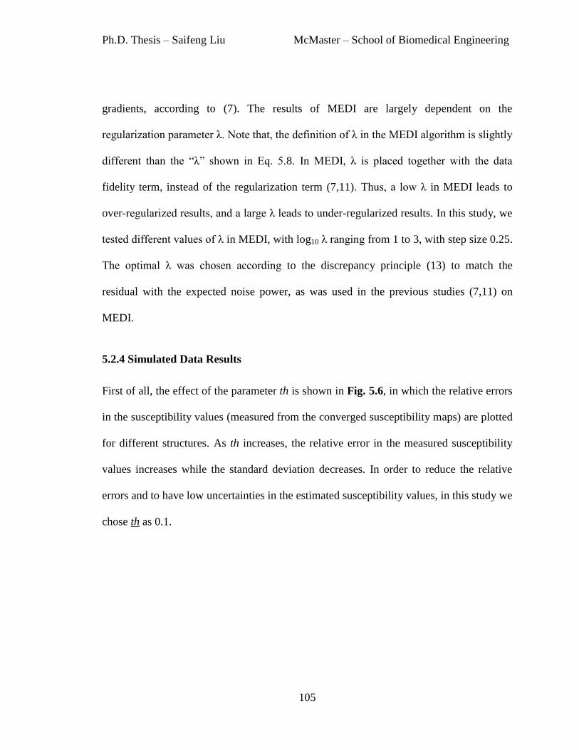
Ph.D. Thesis – Saifeng Liu McMaster – School of Biomedical Engineering
105
gradients, according to (7). The results of MEDI are largely dependent on the
regularization parameter λ. Note that, the definition of λ in the MEDI algorithm is slightly
different than the “λ” shown in Eq. 5.8. In MEDI, λ is placed together with the data
fidelity term, instead of the regularization term (7,11). Thus, a low λ in MEDI leads to
over-regularized results, and a large λ leads to under-regularized results. In this study, we
tested different values of λ in MEDI, with log10 λ ranging from 1 to 3, with step size 0.25.
The optimal λ was chosen according to the discrepancy principle (13) to match the
residual with the expected noise power, as was used in the previous studies (7,11) on
MEDI.
5.2.4 Simulated Data Results
First of all, the effect of the parameter th is shown in Fig. 5.6, in which the relative errors
in the susceptibility values (measured from the converged susceptibility maps) are plotted
for different structures. As th increases, the relative error in the measured susceptibility
values increases while the standard deviation decreases. In order to reduce the relative
errors and to have low uncertainties in the estimated susceptibility values, in this study we
chose th as 0.1.

Ph.D. Thesis – Saifeng Liu McMaster – School of Biomedical Engineering
106
Figure 5.6 The effects of the parameter th on the accuracies of the estimated
susceptibilities of different structures. a) The relative errors (absolute values) in the
measured mean susceptibilities at different values of th. b) The standard deviations of the
measured susceptibilities at different values of th.
Next, the mean and standard deviations of the susceptibilities of different structures at
different iteration steps were plotted in Fig. 5.7. When only the geometries of the veins
were used as constraints, the relative error in the mean susceptibility value of the veins
quickly decreases and converges after the 3rd
iteration, while the relative errors for all the
other structures were increasing, as shown in Fig. 5.7.a. When the geometries of all the
structures, including the veins, were used in the iterative SWIM algorithm, reduced
relative errors in the measured susceptibility values were observed for all the structures,
as indicated in Fig. 5.7.b. For the veins, the relative error was maintained at the same
level as in Fig. 5.7.a. The standard deviations were reducing as more iteration steps were
conducted, as can be seen from Figure 5.7.c to 5.7.f.

Ph.D. Thesis – Saifeng Liu McMaster – School of Biomedical Engineering
107
Figure 5.7 Means and standard deviations of the susceptibility values of different
structures in the 3D brain model at different iteration steps. a and b: the mean
susceptibility values measured at different iteration steps. c to f: the standard deviations
measured at different iteration steps. The images in the first column (a, c and e) show the
changes in mean and standard deviation when a high χth was used in geometry extraction,
while the images in the second column show the results when a low χth was used in
geometry extraction.

Ph.D. Thesis – Saifeng Liu McMaster – School of Biomedical Engineering
108
The iterative SWIM algorithm has reduced the streaking artefacts effectively, as can be
seen from Fig. 5.8. Nonetheless, this iterative algorithm is optimized for the veins and the
selected grey matter structures only. For the other parts of the brain, the relative errors in
the measured mean susceptibility values were slightly increased after the iterative SWIM
algorithm, as indicated by the error maps shown in Fig. 5.8.c and 5.8.d.
Figure 5.8 a) The initial susceptibility map. b) The final susceptibility map after iterative
SWIM. c) The difference between a and the ideal susceptibility map. d) The difference
between b and the ideal susceptibility map.

Ph.D. Thesis – Saifeng Liu McMaster – School of Biomedical Engineering
109
Figure 5.9 K-space profiles of the initial susceptibility map (a) and the final
susceptibility map after iterative SWIM algorithm (b). The errors in the k-space profiles
in a and b are shown in c and d, respectively. Specifically, the errors were calculated by
comparing the k-space of the generated susceptibility maps with the kspace of the ideal
susceptibility maps. Compared with the initial susceptibility maps, the final susceptibility
maps after iterative SWIM algorithm have reduced errors in the cone of singularities in k-
space, as indicated by the white arrows.
The k-space profiles of the original susceptibility map and the final susceptibility map
after iterative SWIM algorithm are shown in Fig. 5.9. The errors of k-space data in the
cone of singularity regions were reduced after the iterative SWIM algorithm, especially
for the central part of the k-space, as indicated by the white arrows in Fig. 5.9.

Ph.D. Thesis – Saifeng Liu McMaster – School of Biomedical Engineering
110
5.2.5 In vivo Data Results
Figure 5.10 The extracted geometries of veins and grey matter structures (a and b) and
the susceptibility maps (c and d) for the in vivo data. a) Maximum intensity projection of
the binary masks of veins extracted using a high χth. b) One slice of the binary masks of
the grey matter structures extracted using a low χth. c) Maximum intensity projection of
the initial susceptibility maps. d) The corresponding susceptibility map to the binary
mask shown in b.
The vein masks obtained from the in vivo data are shown in Fig. 5.10. Particularly, Fig.
5.10.a shows the maximum intensity projection (MIP) of the binary vein masks obtained
from single high-pass filtering and thresholding, while Fig. 5.10.b shows the one slice of
the binary masks for other grey matter structures with lower susceptibility values than the

Ph.D. Thesis – Saifeng Liu McMaster – School of Biomedical Engineering
111
veins. In order to evaluate the accuracy in the structure extraction, the vein masks and
grey matter structure masks were generated for the brain model using the same algorithms
and parameters. The relative error (calculated as (number of missed pixels +number of
false positives) / actual number pixels in veins) in the extracted veins was measured as 9%
and 10%, respectively. For the in vivo data, it was also observed that, the detected
geometries of the veins or grey matter structures were sometimes locally contaminated by
the noise and streaking artefacts which may have high intensities on the susceptibility
maps. Besides, the putamen was only partly extracted, as shown in Fig. 5.10.b. This
could be due to the variation of susceptibilities within the putamen.
Similar to what was seen in the simulation, in the first round of iterations, when the
geometries of the veins were extracted using the high , the mean susceptibility values
of veins quickly converge after the 3rd
iteration step, as shown in Fig. 5.11.a. The
susceptibility values of other structures were decreased after the iterative algorithm was
applied, except for red nucleus, for which the susceptibility value was slightly increased,
as indicated by the images in the first columns of Figs. 5.11 and 5.12. In the second round
of iterations, when the geometries of both the grey matter structures and the veins were
extracted using a low , the mean susceptibility values of all the grey matter structures
were increased, while the susceptibility of the veins was maintained at the same level as
in the first round of iterations, as can be seen from the second columns of Figs. 5.11 and
5.12. For the veins, the standard deviations in the measured susceptibilities were
decreased as more iteration steps were conducted, as shown in Fig. 5.13.a and 5.13.b. For
other structures, the standard deviations measured in the second round of iterations were

Ph.D. Thesis – Saifeng Liu McMaster – School of Biomedical Engineering
112
slightly increased (Fig. 5.13.c and 5.13.d). This could be caused by the errors in the
extracted geometries of these structures. The streaking artefacts were reduced
dramatically for all the structures, as can be seen from Fig. 5.14.
Figure 5.11 Mean susceptibility values of veins and globus pallidus at different iteration
steps in the in vivo data. The figures in the first column were obtained when high χth was
used to extract the geometries of veins only, while the figures in the second column were
measured when low χth was used to extract the geometries of veins and other structures.

Ph.D. Thesis – Saifeng Liu McMaster – School of Biomedical Engineering
113
Figure 5.12 Mean susceptibility values of red nucleus (RN), caudate nucleus (CN) and
putamen (PUT) at different iteration steps in the in vivo data. The figures in the first
column were obtained when high χth was used to extract the geometries of veins only,
while the figures in the second column were measured when low χth was used to extract
the geometries of veins and other structures.

Ph.D. Thesis – Saifeng Liu McMaster – School of Biomedical Engineering
114
Figure 5.13 Standard deviations of the susceptibility values at different iteration steps for
different structures in the in vivo data. The figures in the first column were obtained when
high χth was used to extract the geometries of veins only, while the figures in the second
column were measured when low χth was used to extract the geometries of veins and other
structures.

Ph.D. Thesis – Saifeng Liu McMaster – School of Biomedical Engineering
115
Figure 5.14 Comparison between the initial susceptibiltiy maps (a and d) and the final
susceptibility maps (b and e). Their differences are shown in c and f (generated as b-a
and e-d).
5.2.6 Comparison with Morphology Enabled Dipole Inversion (MEDI)
For MEDI, the proper value of λ was selected based on Fig. 5.15. The susceptibility maps
generated with different values of λ are shown in Fig. 5.16. The smaller the λ, the more
smoothed the susceptibility maps, and the smaller the RMSE. In this study, the optimal λ
was chosen to be 100.
Compared with the susceptibility maps generated by iterative SWIM algorithm, MEDI
leads to smoother images with preserved edge information in the predefined regions.
However, since MEDI utilizes the edge information in magnitude images only, when
there is no clear edge, MEDI may lead to underestimation of the susceptibilities of veins,
as shown in Fig. 5.17. In the cortical region, these two methods yield similar results.

Ph.D. Thesis – Saifeng Liu McMaster – School of Biomedical Engineering
116
Figure 5.15 The effects of the regularization parameter λ in MEDI. The average gradient
was measured in the low gradient regions in the converged susceptibility maps.
Figure 5.16 Susceptibility maps generated using different values of regularization
parameter λ with MEDI. a and d: λ=10. b and e: λ=100. a and d: λ=1000.

Ph.D. Thesis – Saifeng Liu McMaster – School of Biomedical Engineering
117
Figure 5.17 Comparison of susceptibility maps generated by iterative SWIM (a) and
MEDI (b). The profiles of the solid black lines across the vein of Galen in a and b are
shown in c. The profiles of the dashed black line in the cortical region were shown in d.
The corresponding magnitude image is shown in e, which does not have clear edge
information of the veins in the region indicated by the white arrow.
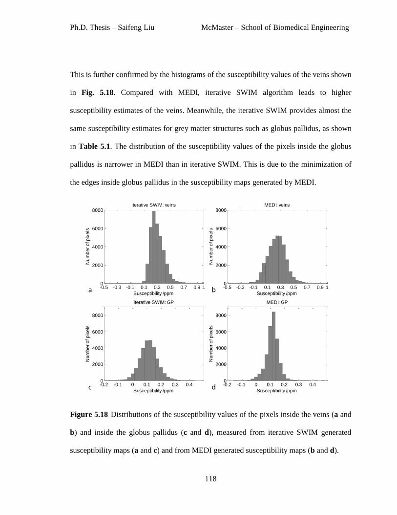
Ph.D. Thesis – Saifeng Liu McMaster – School of Biomedical Engineering
118
This is further confirmed by the histograms of the susceptibility values of the veins shown
in Fig. 5.18. Compared with MEDI, iterative SWIM algorithm leads to higher
susceptibility estimates of the veins. Meanwhile, the iterative SWIM provides almost the
same susceptibility estimates for grey matter structures such as globus pallidus, as shown
in Table 5.1. The distribution of the susceptibility values of the pixels inside the globus
pallidus is narrower in MEDI than in iterative SWIM. This is due to the minimization of
the edges inside globus pallidus in the susceptibility maps generated by MEDI.
Figure 5.18 Distributions of the susceptibility values of the pixels inside the veins (a and
b) and inside the globus pallidus (c and d), measured from iterative SWIM generated
susceptibility maps (a and c) and from MEDI generated susceptibility maps (b and d).
-0.5 -0.3 -0.1 0.1 0.3 0.5 0.7 0.9 10
2000
4000
6000
8000iterative SWIM: veins
Susceptibility /ppm
Nu
mb
er
of p
ixe
ls
-0.5 -0.3 -0.1 0.1 0.3 0.5 0.7 0.9 10
2000
4000
6000
8000MEDI: veins
Susceptibility /ppm
Nu
mb
er
of p
ixe
ls
-0.2 -0.1 0 0.1 0.2 0.3 0.40
2000
4000
6000
8000
iterative SWIM: GP
Susceptibility /ppm
Nu
mb
er
of p
ixe
ls
-0.2 -0.1 0 0.1 0.2 0.3 0.40
2000
4000
6000
8000
MEDI: GP
Susceptibility /ppm
Nu
mb
er
of p
ixe
ls
a b
c d

Ph.D. Thesis – Saifeng Liu McMaster – School of Biomedical Engineering
119
Table 5.1 Mean and standard deviation (in ppm) measured from susceptibility maps
generated using iterative SWIM algorithm and MEDI.
Iterative SWIM MEDI
Vein 0.30±0.11 0.24±0.15
Globus Pallidus 0.11±0.06 0.12±0.04
Red Nucleus 0.05±0.05 0.06±0.03
Caudate Nucleus 0.04±0.05 0.04±0.03
Putamen 0.02±0.05 0.03±0.04
The k-space profiles of the susceptibility maps are shown in Fig. 5.19. The major
difference between the k-space obtained from MEDI and the k-space generated by
iterative SWIM is associated with the singularity regions in k-space. For the k-space
generated using iterative SWIM algorithm, the lower amplitude inside the singularity
regions is due to the fact that only veins and certain grey matter structures with high
susceptibility values were used to update the k-space. It can also be observed that outside
the singularity regions, the amplitude of the k-space generated by iterative SWIM is
slightly higher than that generated by MEDI, as indicated by the white arrow in Fig.
5.19.d. This is due to the difference between MEDI and iterative SWIM in defining the
cone of singularities. In iterative SWIM, the cone of singularities is explicitly defined
using the k-space truncation threshold, and only the k-space data inside this singularity
region are updated.
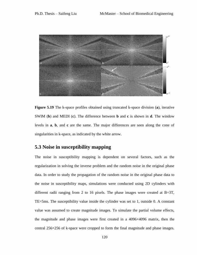
Ph.D. Thesis – Saifeng Liu McMaster – School of Biomedical Engineering
120
Figure 5.19 The k-space profiles obtained using truncated k-space division (a), iterative
SWIM (b) and MEDI (c). The difference between b and c is shown in d. The window
levels in a, b, and c are the same. The major differences are seen along the cone of
singularities in k-space, as indicated by the white arrow.
5.3 Noise in susceptibility mapping
The noise in susceptibility mapping is dependent on several factors, such as the
regularization in solving the inverse problem and the random noise in the original phase
data. In order to study the propagation of the random noise in the original phase data to
the noise in susceptibility maps, simulations were conducted using 2D cylinders with
different radii ranging from 2 to 16 pixels. The phase images were created at B=3T,
TE=5ms. The susceptibility value inside the cylinder was set to 1, outside 0. A constant
value was assumed to create magnitude images. To simulate the partial volume effects,
the magnitude and phase images were first created in a 4096×4096 matrix, then the
central 256×256 of k-space were cropped to form the final magnitude and phase images.

Ph.D. Thesis – Saifeng Liu McMaster – School of Biomedical Engineering
121
Random noise was added to real and imaginary channels of the complex data, and the
SNR in the magnitude images ranged from 2:1 to 20:1.
The susceptibility maps were generated using truncated k-space division, with k-space
truncation threshold th ranging from 0.01 to 0.66, with step size 0.01. In order to study
the propagation of random noise, independent of different regularization algorithms, the
singularity regions where were replaced using the k-space data of the ideal
susceptibility maps. Means and standard deviations of susceptibility values were
measured from both the regions inside the cylinders and a referenced region in the
background. The mean susceptibility values were used to calculate the relative error in
susceptibility estimation using different regularization thresholds with different levels of
noise, while the standard deviations were used to estimate the noise in the susceptibility
maps.
As shown in Fig. 5.20.a and b, the standard deviations measured in the reference region
in the background are consistent for different cylinders. However, the standard deviations
measured inside the cylinders show large variation. For large cylinders, the standard
deviations measured in the two different regions are similar. Thus, the large difference
between the standard deviations in Fig. 5.20.a and b for small cylinders is mainly due to
the partial volume effects. When the standard deviations measured in the background
reference region was used in analysis, the noise in susceptibility maps is found to be
dependent on the noise in the original phase images. This relation can be approximated as
a linear function as:
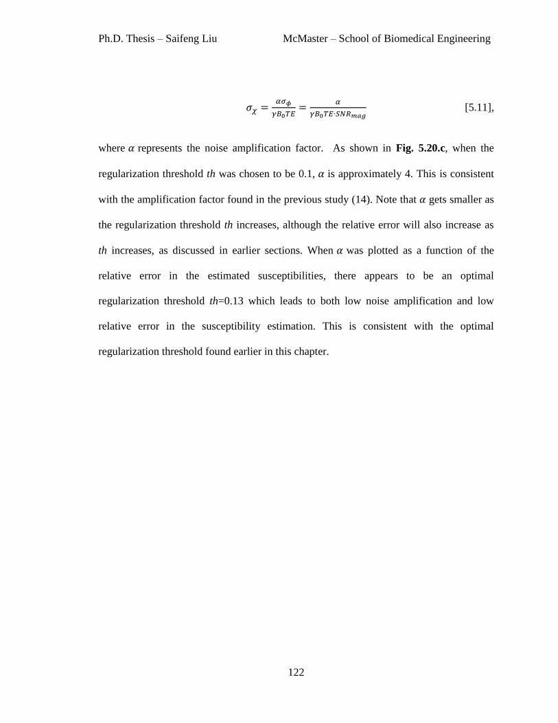
Ph.D. Thesis – Saifeng Liu McMaster – School of Biomedical Engineering
122
[5.11],
where represents the noise amplification factor. As shown in Fig. 5.20.c, when the
regularization threshold th was chosen to be 0.1, is approximately 4. This is consistent
with the amplification factor found in the previous study (14). Note that gets smaller as
the regularization threshold th increases, although the relative error will also increase as
th increases, as discussed in earlier sections. When was plotted as a function of the
relative error in the estimated susceptibilities, there appears to be an optimal
regularization threshold th=0.13 which leads to both low noise amplification and low
relative error in the susceptibility estimation. This is consistent with the optimal
regularization threshold found earlier in this chapter.

Ph.D. Thesis – Saifeng Liu McMaster – School of Biomedical Engineering
123
Figure 5.20 a) Standard deviation of susceptibilities measured in the background
reference region for cylinders with different radii. b) Standard deviation measured inside
the cylinders. c) Noise amplification factor α as a function of SNR in magnitude images,
when th=0.1. d) Noise amplification factor α as a function of relative errors in the
estimated susceptibilities, when SNR=10:1. The arrow shows the case when th=0.13,
α=3.3 and the underestimation of the susceptibility is 11.3%.

Ph.D. Thesis – Saifeng Liu McMaster – School of Biomedical Engineering
124
5.4 Discussion and Conclusions
The main obstacle of quantitative susceptibility mapping originates from the ill-posed
inverse problem. This leads to mainly three problems: underestimation of the
susceptibility, streaking artefacts, and amplification of the noise.
The underestimation of susceptibility can be well-approximated for structures with
relatively large susceptibility values, such as veins. But for other structures, such as the
grey matter structures, the estimation of susceptibilities is affected by the streaking
artefacts caused by the nearby strong susceptibility structures. In this case, using a scaling
factor to reduce the underestimation may lead to large uncertainties. Furthermore, it was
noticed that when a large k-space truncation threshold was used, there tends to be more
blurring of the susceptibility maps (4,5).
Another problem of current susceptibility mapping technique is related to the streaking
artefacts. The inverse problem can be efficiently solved in Fourier domain through
truncated k-space division, and the streaking artefacts are related to the regularization that
is applied in the k-space division. Newer techniques aim to map the susceptibilities as an
optimization problem, and impose different constraints to the inverse problem. The
accuracies of these newer methods are largely dependent on the constraints that are used
in the optimization. It has already been shown that purely the gradient information
extracted from magnitude images may not be sufficient, as not all the edges in
susceptibility maps correspond to detectable edges in the magnitude images (8). This is
partly solved by integrating the gradient information found in both magnitude and phase

Ph.D. Thesis – Saifeng Liu McMaster – School of Biomedical Engineering
125
images (8). Essentially, all of these methods fall into the category of edge preserving
smoothing. Even though the susceptibility maps generated by these algorithms are smooth,
the computation time can be prohibitively long. The k-space/image domain iterative
SWIM algorithm, on the other hand, is much faster and more suitable for clinical settings.
For the in vivo data in this study, which has 512x512x256 matrix size, it took MEDI 1.9
hours to converge, but merely 1.6 minutes for iterative SWIM algorithm, on the same
desktop with Intel i7 CPU.
The effectiveness of the iterative SWIM algorithm was also examined using simulated
data and in vivo data. The iterative SWIM algorithm has replaced the original k-space
data in the cone of singularities, using the k-space of high-susceptibility structures. This
results in proper interpolation of the missing data in central part of the k-space, and
suppression of the noise with high frequency due to the replacing of missing data in the
periphery of k-space. The iterative SWIM algorithm preserves the susceptibility
information of the veins, but may potentially under-estimate the susceptibility of bigger
grey matter structures, if they are not included in the geometry masks. Nonetheless, the
streaking artefacts surrounding the veins were largely reduced together with improved
accuracy of estimating the susceptibility of the veins. This is particularly advantageous
for studies related to measuring venous oxygen saturation.
Finally, the propagation of the random noise from original phase images to susceptibility
maps was studied. With typical truncation threshold of 0.1, the noise amplification factor
is close to four. This amplification factor was obtained assuming that only the cone of
singularities in k-space was updated or modified. There are also studies on the noise

Ph.D. Thesis – Saifeng Liu McMaster – School of Biomedical Engineering
126
behavior in susceptibility mapping, using algorithms that update all the k-space values
(15). Due to the smoothing function used in these algorithms, it is expected that the noise
will be reduced in susceptibility maps.
The accuracy of susceptibility mapping is also affected by many other factors,
particularly, partial volume effects. While this is less a problem for relatively big
structures such as the globus pallidus, with the resolution used clinically (e.g., 1mm x
1mm x 2mm), it may cause errors for the veins. Considering a vein with diameter close to
the imaging resolution, it may be still feasible to obtain a susceptibility value for the pixel
which contains the vein. However, due to partial volume effects, it is not possible to
obtain an accurate susceptibility value for the vein itself, but only an estimate of the
magnetic moment, unless certain a priori information about the size of the vein is
available (16,17).
In conclusion, the core of quantitative susceptibility mapping is solving the inverse
problem. Various algorithms have been proposed to deal with the ill-posedness of this
inverse problem. The k-space/image domain iterative algorithm is particularly time-
efficient and applicable, especially for studies focused on measuring venous oxygen
saturation.

Ph.D. Thesis – Saifeng Liu McMaster – School of Biomedical Engineering
127
References
1. Salomir R, de Senneville BD, Moonen CT. A fast calculation method for magnetic
field inhomogeneity due to an arbitrary distribution of bulk susceptibility. Concepts
Magn. Reson. Part B Magn. Reson. Eng. 2003;19B:26–34.
2. Marques J p., Bowtell R. Application of a Fourier-based method for rapid
calculation of field inhomogeneity due to spatial variation of magnetic susceptibility.
Concepts Magn. Reson. Part B Magn. Reson. Eng. 2005;25B:65–78.
3. Cheng Y-CN, Neelavalli J, Haacke EM. Limitations of calculating field distributions
and magnetic susceptibilities in MRI using a Fourier based method. Phys. Med. Biol.
2009;54:1169–89.
4. Haacke EM, Tang J, Neelavalli J, Cheng YC. Susceptibility mapping as a means to
visualize veins and quantify oxygen saturation. J. Magn. Reson. Imaging
2010;32:663–76.
5. Shmueli K, de Zwart JA, van Gelderen P, Li T, Dodd SJ, Duyn JH. Magnetic
susceptibility mapping of brain tissue in vivo using MRI phase data. Magn. Reson.
Med. 2009;62:1510–22.
6. Schweser F, Deistung A, Sommer K, Reichenbach JR. Toward online reconstruction
of quantitative susceptibility maps: superfast dipole inversion. Magn. Reson. Med.
2013;69:1582–94.
7. Liu J, Liu T, de Rochefort L, Ledoux J, Khalidov I, Chen W, et al. Morphology
enabled dipole inversion for quantitative susceptibility mapping using structural
consistency between the magnitude image and the susceptibility map. NeuroImage
2012;59:2560–8.
8. Schweser F, Sommer K, Deistung A, Reichenbach JR. Quantitative susceptibility
mapping for investigating subtle susceptibility variations in the human brain.
NeuroImage 2012;62:2083–100.
9. Bilgic B, Pfefferbaum A, Rohlfing T, Sullivan EV, Adalsteinsson E. MRI estimates
of brain iron concentration in normal aging using quantitative susceptibility mapping.
NeuroImage 2012;59:2625–35.
10. Paige CC, Saunders MA. LSQR: An Algorithm for Sparse Linear Equations and
Sparse Least Squares. ACM Trans Math Softw 1982;8:43–71.
11. Liu T, Wisnieff C, Lou M, Chen W, Spincemaille P, Wang Y. Nonlinear
formulation of the magnetic field to source relationship for robust quantitative
susceptibility mapping. Magn. Reson. Med. 2013;69:467–76.
12. Perona P, Malik J. Scale-space and edge detection using anisotropic diffusion. IEEE
Trans. Pattern Anal. Mach. Intell. 1990;12:629–39.
13. Morozov, VA. On the solution of functional equations by the method of
regularization. Sov. Math Dokl 1966;7:414–7.
14. Tang J, Liu S, Neelavalli J, Cheng YCN, Buch S, Haacke EM. Improving
susceptibility mapping using a threshold-based K-space/image domain iterative
reconstruction approach. Magn. Reson. Med. 2013;69:1396–407.

Ph.D. Thesis – Saifeng Liu McMaster – School of Biomedical Engineering
128
15. Liu T, Xu W, Spincemaille P, Avestimehr AS, Wang Y. Accuracy of the
morphology enabled dipole inversion (MEDI) algorithm for quantitative
susceptibility mapping in MRI. IEEE Trans. Med. Imaging 2012;31:816–24.
16. Cheng Y-C, Hsieh C-Y, Neelavalli J, Haacke EM. Quantifying effective magnetic
moments of narrow cylindrical objects in MRI. Phys. Med. Biol. 2009;54:7025–44.
17. Liu S, Neelavalli J, Cheng Y-CN, Tang J, Mark Haacke E. Quantitative
susceptibility mapping of small objects using volume constraints. Magn. Reson.
Med. 2013;69:716–23.

Ph.D. Thesis – Saifeng Liu McMaster – School of Biomedical Engineering
129
Chapter 6 Improved Venography
using True Susceptibility Weighted
Imaging (tSWI)2
6.1 Introduction
Susceptibility weighted imaging (SWI) is a high resolution, spoiled gradient echo (GRE)
magnetic resonance imaging (MRI) technique used today clinically for evaluating small
veins and venous abnormalities in the brain and the presence of increased iron content
and microbleeds in diseases such as dementia, multiple sclerosis (MS), Parkinson’s
disease, stroke and traumatic brain injury (TBI) (1–3). SWI's exquisite sensitivity to small
tissue magnetic susceptibility changes is due to its use of phase information (3–5).
Paramagnetic or diamagnetic substances relative to water such as blood products or
calcium, respectively, perturb the local magnetic field proportional to their respective
magnetic susceptibilities. These differences are reflected in the phase of the MR images.
2Most of the contents in this chapter are adapted from Liu S, Mok K, Neelavalli J, Cheng YCN, Tang J, Ye
Y, Haacke EM. Improved MR Venography Using Quantitative Susceptibility-Weighted Imaging. J. Magn.
Reson. Imaging 2013; Article first published online: 31 OCT 2013 DOI: 10.1002/jmri.24413. Reprint under
license.

Ph.D. Thesis – Saifeng Liu McMaster – School of Biomedical Engineering
130
In conventional SWI, after applying appropriate unwrapping and/or filtering techniques
on the raw phase data (1,3), a phase dependent mask is created and multiplied n times into
the magnitude data to enhance the contrast/visibility of these substances.
Although SWI has been used quite successfully in clinical applications for many years, it
is important to realize that it has a few weaknesses. One of them is based on the fact that
the MRI phase signal is not only a function of the susceptibility, but also dependent on
shape and orientation of the structure of interest. In data acquired with sufficient
resolution, the phase inside veins perpendicular to the field has the opposite sign to that
inside veins parallel to B0. This leads to variable suppression effects with the phase mask
that makes SWI unique over conventional gradient echo imaging (6). Recently,
quantitative susceptibility mapping (QSM) has emerged as a means to extract the source
of phase information, that is, the local susceptibility distribution (7–15). QSM is known to
be independent of echo time and, to a large degree, of orientation. To avoid the vessel
orientation dependence in routine SWI data, instead of phase, we propose using a mask
based on the susceptibility map. We refer to this approach as true-SWI (tSWI) to
distinguish it from the conventional phase mask based SWI. In this work, our purpose is
to compare the ability of these two methods to improve venous contrast and to show that
tSWI is able to remove the geometry dependence of the phase for veins and microbleeds
in SWI data.

Ph.D. Thesis – Saifeng Liu McMaster – School of Biomedical Engineering
131
6.2 Materials and Methods
To provide some flexibility in generating the susceptibility weighting mask W, we
introduce both lower and upper thresholds for defining the mask as follows:
{
[6.1],
where refers to the susceptibility value of a voxel (e.g., vein) relative to the surrounding
tissue in the susceptibility map, is the lower limit and is the upper limit of the range
of tissue susceptibility values for which we want to improve the contrast in the final
susceptibility weighted image. Finally, the true-SWI is generated by multiplying the
magnitude image with the mask n times similar to the usual SWI mask application:
[6.2].
The whole process is illustrated in Fig.6.1.
In order to determine appropriate values for these two thresholds, we examined different
potential choices. For , we used: 1) the mean susceptibility value in the background
white matter tissue region (0 ppm) in the susceptibility map and 2) three standard
deviations ( ) above the tissue region, where is the standard deviation of the white
matter tissue region in the susceptibility map. While a threshold of 0 ppm would ensure
that the susceptibility weighting mask would include smaller veins that are partial
volumed, it can also lead to increased noise in tissue regions where susceptibility is
supposed to be zero. On the other hand, a choice of would reduce inclusion of
noise in the mask. For , we used: 1) the expected mean susceptibility value in the vein,

Ph.D. Thesis – Saifeng Liu McMaster – School of Biomedical Engineering
132
which is about 0.45 parts per million (ppm) relative to water (3,16) under normal
physiological conditions; and 2) a value higher than this, in this case 1ppm.
Figure 6.1 A comparison between tSWI and SWI data processing steps.

Ph.D. Thesis – Saifeng Liu McMaster – School of Biomedical Engineering
133
For a given set of and values, the contrast-to-noise ratio (CNR) between the vein
and the background tissue can be optimized by choosing an appropriate n value in Eq. 6.2.
CNR for a vein can be defined as the ratio between tSWI signal contrast for the vein and
its associated uncertainty as follows:
[6.3],
where √
. Noise in either the reference (background tissue)
region ( ) or in the vein ( ) in the tSWI image can be estimated using the
following equation:
√
[6.4].
The noise, represented by the standard deviation for a given voxel in W, , is dependent
on the noise, , in the susceptibility map in the following manner:
{
[6.5].
The factor 1/2 in the case when or in Eq. 6.5 is due to the discontinuity (1).
For simplicity, we assume that signal from vein (or cylinder) and reference region in the
original magnitude images are the same: , and their associated
signal standard deviations in these two regions are also the same:
. Furthermore, we assume that the mean susceptibility value of the reference region is 0,
and the mean susceptibility value of the vein is .

Ph.D. Thesis – Saifeng Liu McMaster – School of Biomedical Engineering
134
i) When a threshold of = 0 was used to generate the susceptibility mask, in the
reference region, W = 1, and . In the vein, W = , ,
for ; but when , W = 0, ; when , W =
0, = 0. Using Eq. 6.4,
{
(
(
)
(
)
)
(
)
(
)
[6.6].
ii) When a threshold of was chosen, in the reference region, W = 1, and = 0
due to the fact that most pixels in the reference (background tissue) region have
susceptibility values less than . In the vein, W = ,
, for ; but when , W = 0, ;
when , W = 0, = 0. Thus,
{
( (
)
(
)
( ) )
(
( ) )
[6.7].
Thus the CNR can be written as:

Ph.D. Thesis – Saifeng Liu McMaster – School of Biomedical Engineering
135
(
)
[6.8],
for , with given in Eqs. 6.6 and 6.7.
When and is slightly less than , CNR approaches SNR in the magnitude
images as n approaches infinity. In this case, the optimal n was chosen to be the value
where CNR reaches 90% of the maximal CNR for a certain vein.
Simulations
To evaluate the theoretical predictions, the optimal choice of n for generating tSWI
images for different threshold values and vessel susceptibility values, and the influence of
high-pass filtering on the final CNR for veins in tSWI images, simulations were
performed using cylinders as surrogates to veins. A series of cylinders with radii ranging
from 2 pixels to 16 pixels was used to simulate the associated phase images in a 512×512
matrix at B0=3T, and TE=10ms. The cylinders were taken to be perpendicular to the main
magnetic field. The input susceptibility of the cylinders was set to be 0.45ppm and the
susceptibility value of the background region was set to zero. In order to simulate a more
realistic response of the field perturbation, the complex data of a cylinder with radius 16
times of the final radius was first created on an 8192×8192 matrix. The magnitude signal
for the cylinder and background region were taken to be unity. The central 512×512 k-
space points generated from the larger matrix were then used to reconstruct the complex
images of the cylinders. Gaussian noise was added to both real and imaginary channels of
the data to simulate the SNR in the magnitude images to be 10:1. The simulated phase
images were processed using a homodyne high-pass filter with a k-space window size of

Ph.D. Thesis – Saifeng Liu McMaster – School of Biomedical Engineering
136
64×64. Two sets of susceptibility maps, one from unfiltered and the other from filtered
phase images, were generated for each cylinder size, using truncated k-space division
with a k-space threshold of 0.1 (7). This is to evaluate the influence of high-pass filtering
on the final CNR in tSWI images. The tSWI images were generated using Eqs. 6.1 and
6.2 for different values of and as mentioned in the previous section. The standard
deviation of the susceptibility maps was measured from a reference region outside the
cylinder. The susceptibility mask was multiplied into the magnitude image n times with n
ranging from 0 to 10 (n=0 refers to the case of no mask multiplication). The local CNRs
between cylinders and the background reference were measured from the tSWI data using:
[6.9]
where Svein and Sref are the mean intensity values inside the cylinder (vein) and inside a
reference region of interest (ROI) adjacent to the cylinder directly from tSWI image,
respectively. In order to estimate the overall noise directly from tSWI images, the
standard deviations inside the cylinder ( ) and the reference region ( ) in
tSWI were measured and was again calculated as the square root of
. The theoretically predicted CNRs from Eq. 6.8 using different thresholds for
generating the susceptibility mask were compared with those measured from the
simulations and the appropriate value for for processing in vivo data was determined.
CNRs of the cylinders with different susceptibility values ranging from 0.2ppm to
0.45ppm were calculated to evaluate the influence of the susceptibility value of the object
on the optimal choice of n.

Ph.D. Thesis – Saifeng Liu McMaster – School of Biomedical Engineering
137
In vivo data
Table 6.1 Imaging parameters for three volunteers and one patient for in vivo studies.
Dataset 5 was collected on a TBI patient.
To evaluate the efficacy of tSWI in in vivo neuro-imaging, we compared the CNR
obtained in tSWI data with that obtained in conventional SWI images in three healthy
adult volunteers. The study was approved by the local institutional review board and
informed consent was obtained from all subjects before the MRI scan. The volunteers
were imaged on a 3T Verio system (Siemens, Erlangen) using a 3D SWI sequence with
isotropic voxel size of 0.5mm×0.5mm×0.5mm. Imaging parameters are given in Table
6.1. Data were acquired in the transverse orientation. In one case (volunteer 1), the SWI
sequence was performed twice using two different echo times (TE = 14.3ms and 17.3ms).
To evaluate the influence of voxel aspect ratio on the CNR, lower resolution images of
0.5mm×0.5mm×2mm (anisotropic voxel size) from all 4 volunteer datasets were
Dataset No. 1 2 3 4 5
Volunteer No. 1 1 2 3 -
B0 (T) 3 3 3 3 3
TR (ms) 26 26 24 24 29
TE (ms) 14.3 17.3 17 15.3 20
FA (degrees) 15 15 15 12 15
BW (Hz/px) 121 121 181 121 120
Voxel size (mm3)
0.5×0.5
×0.5
0.5×0.5
×0.5
0.5×0.5
×0.5
0.5×0.5
×0.5
0.5×0.5
×2
Matrix Size 512×368
×256
512×368
×256
512×368
×224
512×368
×192
512×416
×64

Ph.D. Thesis – Saifeng Liu McMaster – School of Biomedical Engineering
138
generated by taking the central portion of the original k-space along the transverse
direction.
The quantitative susceptibility maps were generated for the isotropic and the anisotropic
data, as follows: tissues outside the brain were removed using the Brain Extraction Tool
(BET) in FSL (17), a homodyne high-pass filter with a k-space window of 64×64 was
applied to remove the background field induced phase artefacts (1), and the inversion
process to create susceptibility maps was accomplished using a single orientation
truncated k-space division approach with a k-space truncation threshold of 0.1 (7).
Similar to the case of the simulated data, two sets of tSWI images for each of the SWI
datasets were generated using Eqs. 6.1 and 6.2 with: a) =0 and b) , where
is the standard deviation of the susceptibility in the background white matter region close
to the vein for which the CNR was measured. The threshold was kept at 0.45ppm. The
susceptibility mask was multiplied into the magnitude image n times, with n ranging from
1 to 10. To generate conventional SWI images, phase masks were created using the high-
pass filtered phase images and then multiplied four times into the magnitude images (1).
To investigate the impact of newer data processing methods, we also applied phase
unwrapping (18) and SHARP (9) to remove the background field, and applied a geometry
constrained iterative algorithm (8) to reconstruct the susceptibility maps for one dataset
(Dataset 2). Then, tSWI images were generated using =0 and =0.45ppm. Local
CNRs of two selected veins, the left internal cerebral vein (LICV) and the right septal
vein (RSV), were measured from both tSWI and SWI using Eq. 6.9. Each vessel’s ROI
was selected from the susceptibility maps and copied onto the tSWI or SWI images for

Ph.D. Thesis – Saifeng Liu McMaster – School of Biomedical Engineering
139
CNR evaluation. The reference ROI adjacent to each vein was taken from the same slice.
To demonstrate the advantages of using tSWI over conventional SWI, we also analyzed
one SWI dataset from a TBI patient. For this patient dataset, susceptibility maps were
generated through homodyne high-pass filtering and truncated k-space division. tSWI
images were then obtained with susceptibility weighting masks generated using =0,
=0.45ppm and n=2. All the processing was done using Matlab (R2010a, Natick, MA).
6.3 Results
Simulations
The simulated phase images of cylinders of different sizes, their corresponding
susceptibility maps and tSWI images are shown in Fig. 6.2. The measured CNRs for
cylinders with different radii, but with a constant input susceptibility of 0.45ppm, are
plotted as a function of n in Fig. 6.3, and the theoretically predicted CNRs are plotted in
Fig. 6.4. Since no T2* effects are considered here, the CNRs shown in Figs. 6.3 and 6.4
reflect contrasts from only phase/susceptibility differences between the cylinders and the
background reference region. The optimal choice of n and, correspondingly, the value of
CNR in the tSWI image, are influenced both by (a) the choices of and and (b) the
high pass filter. For =0, CNRs reach maximum when n ≤ 4 (Figs. 6.3.a, 6.3.c, 6.3.e,
6.4.a and 6.4.c). When is larger with =0, it also takes a larger n value to reach the
optimized CNR. Meanwhile, the choices of and can also affect the rate at which
optimal CNR is approached as a function of n. For , CNRs in general increase
as n increases (Figs. 6.3.b, 6.3.d, 6.3.f, 6.4.b and 6.4.d). The optimal n may be chosen

Ph.D. Thesis – Saifeng Liu McMaster – School of Biomedical Engineering
140
when CNR reaches 90% of the maximum of CNR. The optimal n was 4 for =0.45ppm,
and greater than 10 for =1ppm.
Figure 6.2 Phase images (a and b), susceptibility maps (c and d) and tSWI images (e, f, g
and h) for simulated cylinders with and without homodyne high-pass filtering. Images in
the first and third columns are generated using the original phase images without high-
pass filtering, while images in the second and fourth columns are generated using high-
pass filtering. The tSWI images e and f were generated using χ1=0, χ2=0.45ppm, n=2;
while g and h were generated using χ1=3σχ, χ2=0.45ppm, n=4. σχ is the standard deviation
of a reference region measured from the susceptibility maps shown in c and d
(σχ=0.05ppm for both c and d). The SNR in the original magnitude image was set to be
10:1 and the CNR between the cylinders and background in the original magnitude
images was basically zero.

Ph.D. Thesis – Saifeng Liu McMaster – School of Biomedical Engineering
141
Figure 6.3 Measured CNRs of cylinders from simulated tSWI images. Figures in
different rows were generated using different χ2 values, while figures in different columns
were generated using different χ1 values. a) χ1=0, χ2=1ppm; b) χ1=3σχ, χ2=1ppm; c) χ1=0,
χ2=0.45ppm; d) χ1=3σχ, χ2=0.45ppm; e) χ1=0, χ2=0.45ppm; and f) χ1=3σχ, χ2=0.45ppm.
To evaluate the effect of high-pass filtering, e and f were generated using high-pass
filtered phase images.

Ph.D. Thesis – Saifeng Liu McMaster – School of Biomedical Engineering
142
Figure 6.4 Theoretically predicted CNRs of cylinders with different susceptibility values.
Figures in different rows were generated using different χ2 values, while figures in
different columns were generated using different χ1 values. a) χ1=0, χ2=1ppm; b) χ1=3σχ,
χ2=1ppm; c) χ1=0, χ2=0.45ppm; and d) χ1=3σχ, χ2=0.45ppm.
When a high-pass filtered phase was used, the optimal choice of n was not affected much
for =0 and = 0.45ppm (Fig. 6.3.e), but was slightly bigger for and =
0.45ppm for all the cylinders except for the smallest one (Fig. 6.3.f). For both = 0
and , the maximal CNR was reduced for bigger cylinders, when the high-pass
filter was used. This is also partly evident in Fig. 6.2. The behavior in the case when the
high pass filtered phase was used, agreed with the pattern observed in the theoretically
predicted CNRs for objects with low susceptibility in Fig. 6.4. Given the simulated results

Ph.D. Thesis – Saifeng Liu McMaster – School of Biomedical Engineering
143
shown in Fig. 6.3, we chose = 0.45ppm in the in vivo studies for a consistent choice of
n for the maximal CNR.
In vivo studies
The local CNRs of the two veins, 1) the right septal vein and 2) the left internal cerebral
vein, normalized by the SNRs, are plotted in Figs. 6.5 and 6.6 for all the in vivo datasets.
The normalized CNRs in the SWI images and in the original magnitude images, as well
as the SNRs in the original magnitude images (from the background tissues) are shown in
Table 6.2. Compared to the original magnitude images, SWI improves the local CNR of
the right septal vein in the anisotropic data, but not in the isotropic data. The CNR of the
left internal cerebral vein is not improved in SWI in either isotropic or anisotropic data,
due to the amplification of the noise in the background tissue region. Compared with the
CNRs in magnitude images, the local CNRs in tSWI were improved by roughly a factor
of 2 in both isotropic and anisotropic cases for = 0. Compared with conventional SWI,
the CNRs were improved by a factor of greater than three for datasets with isotropic
resolution and greater than 30% for datasets with anisotropic resolution in tSWI. The
local CNRs were further improved when . Considering all cases, when = 0
was used, n = 2 was a reasonable practical choice for both isotropic and anisotropic
datasets; when was used, n = 4 was a reasonable choice for isotropic datasets
and n = 8 for anisotropic datasets.

Ph.D. Thesis – Saifeng Liu McMaster – School of Biomedical Engineering
144
Figure 6.5 Local CNRs of the right septal vein (a, c, and e) and the left internal cerebral
vein (b, d, and f) from different datasets with isotropic resolution. a, b, c and d were
generated when threshold χ1=0 was used to create the susceptibility weighting masks,
while e and f were generated when χ1=3σχ was used. The CNRs were normalized by the
corresponding SNRs listed in Table 6.2. c and d show the CNRs of the two veins in
Dataset 2 with isotropic resolution, when different data processing methods were used for
susceptibility mapping (see Fig. 6.7 for examples of the tSWI images).

Ph.D. Thesis – Saifeng Liu McMaster – School of Biomedical Engineering
145
Figure 6.6 Local CNRs of the right septal vein (a, c, and e) and the left internal cerebral
vein (b, d, and f) from different datasets with anisotropic resolution. a, b, c and d were
generated when threshold χ1=0 was used to create the susceptibility weighting masks,
while e and f were generated when χ1=3σχ was used. The CNRs were normalized by the
corresponding SNRs listed in Table 6.2. c and d show the CNRs of the two veins in
Dataset 2 with anisotropic resolution, when different data processing methods were used
for susceptibility mapping (see Fig. 6.7 for examples of the tSWI images).
Ph.D. Thesis – Saifeng Liu McMaster – School of Biomedical Engineering
146
When SHARP along with an iterative algorithm (8) was used to generate susceptibility
maps, the CNRs of the two veins of interest in the corresponding tSWI image were
improved, as shown in Figs. 6.5.c, 6.5.d, 6.6.c and 6.6.d. For isotropic resolution, at n=2
with = 0, the relative improvements for the left internal cerebral vein and the right
septal vein were 23% and 14%, respectively. For anisotropic resolution and at n=2, the
relative improvements for the two veins were less than 5%. However, this improvement
in CNR was more significant for grey matter structures than for veins, as can be seen
from Fig. 6.7.d and 6.7.h.
In Fig. 6.7, we compare the tSWI and SWI minimum intensity projections for both the
isotropic and anisotropic cases. The tSWI appears to have higher CNR than the
conventional SWI in both isotropic and anisotropic data. For tSWI, isotropic data
provided a better delineation of the venous structures, compared to the anisotropic data.
This is consistent with the results shown in Figs. 6.5 and 6.6, in which the normalized
maximal CNRs are higher for the isotropic data than those for the anisotropic data. When
was used, the visibility of some tiny veins and the grey matter structures was
reduced compared to the case when = 0 was used.

Ph.D. Thesis – Saifeng Liu McMaster – School of Biomedical Engineering
147
Figure 6.7 Comparison between minimal intensity projections (mIP) of tSWI and SWI
data over 16mm for isotropic (top row) and anisotropic data (bottom row) for Dataset 2.
For b, c, f and g, susceptibility maps were generated using homodyne high-pass filtering
and thresholded k-space division; while for d and h, susceptibility maps were generated
using SHARP and geometry constrained iterative algorithm. a) isotropic SWI mIP; b)
isotropic tSWI mIP (χ1=0, χ2=0.45ppm, n=2); c) isotropic tSWI mIP (χ1=3σχ,
χ2=0.45ppm, n=4); d) isotropic tSWI mIP (χ1=0, χ2=0.45ppm, n=2); e) anisotropic SWI
mIP. f) anisotropic tSWI mIP (χ1=0, χ2=0.45ppm, n=2). g) anisotropic tSWI mIP (χ1=3σχ,
χ2=0.45ppm, n=8). h) anisotropic tSWI mIP (χ1=0, χ2=0.45ppm, n=2).

Ph.D. Thesis – Saifeng Liu McMaster – School of Biomedical Engineering
148
As an example of this process with = 0, = 0.45ppm and n = 2, Fig. 6.8 shows a
case that demonstrates the problems with the conventional SWI processing: one of the
veins has a trajectory roughly at the magic angle (54.7°) with respect to the direction of
the main magnetic field B0. The black arrow shows the vein which is clearly seen in the
tSWI (Fig. 6.8.f). In SWI (Fig. 6.8.e), the vein actually shows a dark structure which is in
fact more associated with its edges. This makes the veins appear much bigger in the SWI
than in the tSWI data, as can be seen from the minimum intensity projections (mIPs) in
Figs. 6.8.g and 6.8.h. This non-local phase information used in SWI can lead to an
inaccurate estimation of the geometry of microbleeds, as demonstrated in Fig. 6.9. In this
TBI case, tSWI has more faithfully represented the microbleeds.

Ph.D. Thesis – Saifeng Liu McMaster – School of Biomedical Engineering
149
Figure 6.8 A sagittal view showing a vein near the magic angle (54.7° relative to the
main magnetic field) as indicated by the black arrows. a) Phase image (from a left-handed
system) showing effectively zero phase inside the vein, with outer field dipole effects also
visible; b) susceptibility maps showing the vein as uniformly bright; c) susceptibility
weighting mask obtained from the phase image (n=4); d) susceptibility weighting mask
obtained from the susceptibility maps (χ1=0, χ2=0.45ppm, n=2); e) SWI showing
unsuppressed signal inside the vein; and f) tSWI showing a clear suppression of the vein
even at the magic angle. g) mIP of SWI in the sagittal direction. h) mIP of tSWI in the
sagittal direction. Note the vessels near the magic angle are now well delineated in the
tSWI data.

Ph.D. Thesis – Saifeng Liu McMaster – School of Biomedical Engineering
150
Figure 6.9 Sagittal views of SWI (a and c) and tSWI images (b and d) in a TBI case. The
microbleeds appear much bigger on the SWI images than on the tSWI images, as
indicated by the white arrows. This is due to the non-local phase information used in the
conventional SWI weighting mask. For better visualization, the images were interpolated
in through-plane direction from a resolution of 0.5mm×0.5mm×2mm to 0.5mm isotropic
resolution.
6.4 Discussion
Quantitative susceptibility mapping offers an additional means to recognize veins and
microbleeds and other tissues with high iron content as phase imaging does. However, the
phase images are dependent on each object’s shape and orientation while the
susceptibility values of the structures are not, at least in principle. Therefore, to produce

Ph.D. Thesis – Saifeng Liu McMaster – School of Biomedical Engineering
151
better susceptibility weighted images, we have investigated the use of susceptibility maps
for the masking process.
There are a number of key observations that can be made from the data presented herein.
First, the results presented in this paper demonstrate that the object shape and orientation
can be reasonably accounted for by using susceptibility maps and, hence, the inability of
SWI processing to enhance veins at different orientations can be overcome. Besides, the
blooming artefact due to the dipolar phase of microbleeds in conventional SWI was
avoided. This leads to potential applications of this technique, for example, the evaluation
of microbleeds in TBI studies. Nonetheless, the blooming artefact also enables the
visualization of small or even sub-voxel structures using conventional SWI (6). In this
case, due to the severe partial volume effects, the susceptibility values will not be
accurately estimated and it is expected that tSWI will lead to similar results as
conventional SWI. Second, tSWI can be used to process isotropic data, whereas SWI
processing has relied on anisotropic data for its best results due to the direct use of phase
information which is orientation dependent (6). In the past, SWI data have usually been
collected with anisotropic resolution with 2mm slice thickness(6). However, modern
segmented echo planar approaches are becoming viable and one expects to see more data
being collected with isotropic voxel sizes (19,20). The high isotropic resolution also helps
to reduce the error caused by the partial volume effects in susceptibility quantification,
and thus leads to improved quality for tSWI. Note that, high image resolution will also
lead to lower SNR within a given image time and thus lower CNR. Generally speaking,
tSWI is most advantageous with the isotropic datasets. Third, the use of a susceptibility

Ph.D. Thesis – Saifeng Liu McMaster – School of Biomedical Engineering
152
mask is not restricted to the paramagnetic venous blood, but it could also be designed to
study the diamagnetic materials (e.g., calcifications, which have negative susceptibility in
the susceptibility maps). Fourth, the effects of the upper and lower thresholds used in
creating the susceptibility masks have been studied for two reasonable values, and the
optimal number of multiplications, n has been determined. When the lower threshold was
set to zero, the fact that a continuous mask from zero to unity is generated makes it
possible to enhance contrast even in smaller veins, or larger veins that have had their
phase artificially suppressed by using the high-pass filter, or in structures that have lower
iron contents. The use of helps to avoid amplifying noise in regions of low
susceptibility and hence leads to a higher CNR. However, at the same time it can prevent
small veins or structures with very low susceptibility from being enhanced. In addition,
different datasets require different optimal n values. To avoid this problem, it may be
more practical to choose to be 0. We choose the upper threshold to be 0.45ppm, as
it corresponds to the theoretical susceptibility of venous blood when the oxygen
saturation is 70% and the hematocrit is 45%. Increasing this upper threshold may lead to a
slightly larger value for the optimal n when the susceptibility value of the vein is much
smaller than . In most cases, n = 2 gave optimal results, for = 0 and = 0.45ppm.
In order to capture smaller veins or structures with lower susceptibility values such as the
basal ganglia, a slightly larger n can be used for either isotropic or anisotropic datasets
(21). The lower susceptibility values are due to a combined effect of partial volume and
high-pass filtering. Fifth, the predicted CNRs slightly deviate from measured CNRs in
simulations, as the mean value of the susceptibility mask W in the background reference

Ph.D. Thesis – Saifeng Liu McMaster – School of Biomedical Engineering
153
region is slightly less than 1. As a result, this creates slight differences between the
prediction and measurements at large n values (n > 4). Lastly, conventional SWI uses
phase information which is dependent on echo time and usually a relatively long echo
time is used in SWI data collection. Although the phase mask could be redefined as a
function of echo time to accommodate the loss of phase information as echo times are
reduced, no such modification needs to take place for tSWI since the susceptibility map
does not change with echo time. However when echo times are reduced the phase SNR
used to generate the susceptibility map will decrease. On the other hand, if echo times
become too long, phase aliasing occurs and the apparent size of the vessel will increase.
Thus, tSWI makes the use of short echo times possible as long as the SNR is high enough
to create a reasonable estimate of the local susceptibilities. The selection of a shorter TE
has several major advantages, including reducing background field induced phase
artefacts, shorter scan time and better overall image quality.
There are several limitations to this method. First, we are using susceptibility maps
generated from a single orientation dataset to create the mask for tSWI. These
susceptibility maps can have streaking artefacts which are caused by the singularities in
the inverse kernel (7–15). The streaking artefacts could permeate the tSWI data causing
artefacts which did not exist before or decrease the CNR of grey matter structures. Some
newer techniques such as nonlinear regularization (10,13,14) and iterative algorithms (8)
will reduce the streaking artefacts and the latter is particularly time-efficient. Another
common problem of the single orientation QSM method is the systematic under-
estimation or bias of the susceptibility. However, this can be compensated by the

Ph.D. Thesis – Saifeng Liu McMaster – School of Biomedical Engineering
154
thresholds used to generate the tSWI weighting masks. Second, we used the traditional
homodyne high-pass filter to remove the background phase artefacts in the in vivo data.
Even though homodyne high-pass filtering could be applied without phase unwrapping, it
leads to an underestimation of the susceptibility, especially for large objects. This can be
improved by using newly developed background field removal methods (9,22). But for
relatively small structures such as veins, homodyne high-pass filtering already gives
satisfying results if it is performed in the appropriate plane (see Chapter 3). Given the fact
that homodyne high-pass filtering is still being widely used, the proposed algorithm can
be directly added to the current SWI data processing scheme.
In conclusion, we have proposed a data processing scheme which we refer to as true SWI
or tSWI to generate SWI like images using susceptibility maps. This helps to avoid the
orientation dependence related problem in SWI, especially in data with isotropic
resolution and, in the future, possibly to allow the use of short TE SWI data collection.
This tSWI data provide better and more consistent visualization of the venous system and
thus have potential clinical applications in the study of neurodegenerative diseases.

Ph.D. Thesis – Saifeng Liu McMaster – School of Biomedical Engineering
155
References
1. Haacke EM, Xu Y, Cheng YN, Reichenbach JR. Susceptibility weighted imaging
(SWI). Magn. Reson. Med. 2004;52:612–8.
2. Mittal S, Wu Z, Neelavalli J, Haacke EM. Susceptibility-Weighted Imaging:
Technical Aspects and Clinical Applications, Part 2. Am. J. Neuroradiol.
2009;30:232–52.
3. Haacke EM, Reichenbach JR, editors. Susceptibility Weighted Imaging in MRI:
Basic Concepts and Clinical Applications. 1st ed. Wiley-Blackwell; 2011.
4. Haacke EM, Brown RW, Thompson MR, Venkatesan R. Magnetic Resonance
Imaging: Physical Principles and Sequence Design. 1st ed. Wiley-Liss; 1999.
5. Marques J p., Bowtell R. Application of a Fourier-based method for rapid
calculation of field inhomogeneity due to spatial variation of magnetic susceptibility.
Concepts Magn. Reson. Part B Magn. Reson. Eng. 2005;25B:65–78.
6. Xu Y, Haacke EM. The role of voxel aspect ratio in determining apparent vascular
phase behavior in susceptibility weighted imaging. Magn. Reson. Imaging
2006;24:155–60.
7. Haacke EM, Tang J, Neelavalli J, Cheng YC. Susceptibility mapping as a means to
visualize veins and quantify oxygen saturation. J. Magn. Reson. Imaging
2010;32:663–76.
8. Tang J, Liu S, Neelavalli J, Cheng YCN, Buch S, Haacke EM. Improving
susceptibility mapping using a threshold-based K-space/image domain iterative
reconstruction approach. Magn. Reson. Med. 2013;69:1396–407.
9. Schweser F, Deistung A, Lehr BW, Reichenbach JR. Quantitative imaging of
intrinsic magnetic tissue properties using MRI signal phase: An approach to in vivo
brain iron metabolism? NeuroImage 2011;54:2789–807.
10. Schweser F, Sommer K, Deistung A, Reichenbach JR. Quantitative susceptibility
mapping for investigating subtle susceptibility variations in the human brain.
NeuroImage 2012;62:2083–100.
11. Shmueli K, de Zwart JA, van Gelderen P, Li T, Dodd SJ, Duyn JH. Magnetic
susceptibility mapping of brain tissue in vivo using MRI phase data. Magn. Reson.
Med. 2009;62:1510–22.
12. Liu T, Spincemaille P, de Rochefort L, Kressler B, Wang Y. Calculation of
susceptibility through multiple orientation sampling (COSMOS): A method for
conditioning the inverse problem from measured magnetic field map to
susceptibility source image in MRI. Magn. Reson. Med. 2009;61:196–204.
13. Liu J, Liu T, de Rochefort L, Ledoux J, Khalidov I, Chen W, et al. Morphology
enabled dipole inversion for quantitative susceptibility mapping using structural
consistency between the magnitude image and the susceptibility map. NeuroImage
2012;59:2560–8.
14. De Rochefort L, Liu T, Kressler B, Liu J, Spincemaille P, Lebon V, et al.
Quantitative susceptibility map reconstruction from MR phase data using bayesian
regularization: Validation and application to brain imaging. Magn. Reson. Med.
2010;63:194–206.

Ph.D. Thesis – Saifeng Liu McMaster – School of Biomedical Engineering
156
15. Wharton S, Bowtell R. Whole-brain susceptibility mapping at high field: A
comparison of multiple- and single-orientation methods. NeuroImage 2010;53:515–
25.
16. Jain V, Abdulmalik O, Propert KJ, Wehrli FW. Investigating the magnetic
susceptibility properties of fresh human blood for noninvasive oxygen saturation
quantification. Magn. Reson. Med. 2012;68:863–7.
17. Smith SM. Fast robust automated brain extraction. Hum. Brain Mapp. 2002;17:143–
55.
18. Abdul-Rahman HS, Gdeisat MA, Burton DR, Lalor MJ, Lilley F, Moore CJ. Fast
and robust three-dimensional best path phase unwrapping algorithm. Appl. Opt.
2007;46:6623–35.
19. Xu Y, Haacke EM. An iterative reconstruction technique for geometric distortion-
corrected segmented echo-planar imaging. Magn. Reson. Imaging 2008;26:1406–14.
20. Zwanenburg JJM, Versluis MJ, Luijten PR, Petridou N. Fast high resolution whole
brain T2* weighted imaging using echo planar imaging at 7T. NeuroImage
2011;56:1902–7.
21. Gho S-M, Liu C, Li W, Jang U, Kim EY, Hwang D, et al. Susceptibility map-
weighted imaging (SMWI) for neuroimaging. Magn. Reson. Med. 2013; doi:
10.1002/mrm.24920.
22. Liu T, Khalidov I, de Rochefort L, Spincemaille P, Liu J, Tsiouris AJ, et al. A novel
background field removal method for MRI using projection onto dipole fields (PDF).
NMR Biomed. 2011;24:1129–36.

Ph.D. Thesis – Saifeng Liu McMaster – School of Biomedical Engineering
157
Chapter 7 Quantitative Susceptibility
Mapping of Small Objects using
Volume Constraints3
7.1 Introduction
The measurement of magnetic susceptibility offers an entirely new form of contrast in
magnetic resonance imaging (1-6). More specifically, susceptibility quantification has
already found applications in mapping out iron in the form of ferritin in brain tissues such
as the basal ganglia (1, 4, 6) and in the form of deoxyhemoglobin for measuring the
oxygen saturation in veins (1, 4). This new form of imaging may provide a means for
monitoring longitudinal changes in iron content in dementia, multiple sclerosis (MS),
traumatic brain injury (TBI) and Parkinson’s disease (PD). It may also be used to monitor
microbleeds which have been implicated in the progression of vascular dementia (7),
Alzheimer’s and other neurovascular disorders (8, 9).
3Most of the contents in this chapter are adapted from Liu S, Neelavalli J, Cheng Y-CN, Tang J, Haacke
EM. Quantitative susceptibility mapping of small objects using volume constraints. Magn. Reson. Med.
2013;69:716–23. Reprint under license.

Ph.D. Thesis – Saifeng Liu McMaster – School of Biomedical Engineering
158
One of the most recent susceptibility mapping methods is a Fourier based method (2, 3, 5,
10) which utilizes phase images. The accuracy of such a method depends on the volume
measurement of the object. For example, in order to quantify the susceptibility of a given
microbleed, usually the center and the radius of the microbleed have to be determined
(10-13). Alternate volume estimations of the microbleed from high resolution spin echo
images may overcome these limitations. With a gradient echo sequence, the apparent
volume of the object is increased due to what is commonly referred to as the “blooming”
effect, a signal loss around the object caused by T2* dephasing. This increased apparent
volume may be used to obtain an estimated susceptibility of the object while the product
of the apparent volume and the estimated susceptibility is much more robust and should
still provide a good estimate of the magnetic moment of the object.
The goal of this paper is to evaluate the quantitative accuracy of a Fourier based
susceptibility mapping method when it is applied to small structures, and to show that: 1)
an accurate estimate of the magnetic moment is possible using multi-echo gradient echo
imaging; and 2) the accuracy of the effective susceptibility can be improved using the
magnetic moment when an estimate of the true volume is available. For validation, we
used a gel phantom with air bubbles and glass beads to mimic the clinical situation of
microbleeds. The method illustrated here does not depend on the susceptibility value or
the size of the object.

Ph.D. Thesis – Saifeng Liu McMaster – School of Biomedical Engineering
159
7.2 Theory and Methods
Current susceptibility mapping methods are based on the relation between the
susceptibility distribution and the magnetic field variation in the Fourier domain (1-6; 10):
( ) [7.1],
where ( ) is the Fourier transform of the magnetic field variation , is the
Fourier transform of the susceptibility distribution , and is the Green’s
function
[7.2],
assuming that the main field direction is in the z direction. Susceptibility quantification is
an ill-posed inverse problem, due to zeros in the Green’s function along the magic
angle in the k-space domain. As a result, regularization is required. In this study, we
applied the regularization procedure described in a previous study (1) in which the
intensity of the inverse of is reasonably attenuated when the absolute value of
is below a threshold value, th. The selection of this threshold is a trade-off between the
susceptibility-to-noise ratio of the reconstructed susceptibility map and the accuracy in
susceptibility quantification (1, 6). The threshold value was chosen to be 0.1 in this study.
Although ideally is the sought after parameter, when reduced resolution or T2* effects
confound a clean measurement of the object’s volume, it is more appropriate to
investigate the associated magnetic moment (or, equivalently, the total or integrated

Ph.D. Thesis – Saifeng Liu McMaster – School of Biomedical Engineering
160
susceptibility weighted by the voxel volume (12)). To see why this is the case, consider a
sphere with a susceptibility difference , the induced magnetic field at point
outside the sphere is given by (14):
( )
[7.3]
where , is the susceptibility inside the object, is the
susceptibility outside the object, is the radius of the sphere, is the distance from the
point to the center of the sphere, and is the angle between the point P and the
main field direction. For simplicity, the meaning of susceptibility in this paper will be
taken to be rather than or . Eq. 7.3 also indicates that the product is
independent of TE, where is the true volume of the sphere. Since the
magnetic dipole moment of the spherical object is given as (14):
[7.4],
when . For simplicity we refer to the product as the magnetic moment in this
study. The phase value at a particular echo time (TE) is given in a right handed system by:
[7.5].
The susceptibility may be quantified using the phase information, if the true volume
(V) of the object is known. Otherwise, the magnetic moment ( ) may be found. Since
gradient echo images lead to a dephasing artefact and the object appears larger than its
actual size, we defined an apparent volume V′ and assuming that the susceptibility of this

Ph.D. Thesis – Saifeng Liu McMaster – School of Biomedical Engineering
161
larger object can be accurately quantified, the magnetic moment could still be accurately
calculated. Expressed symbolically, an estimated susceptibility value can be
calculated from the Fourier based method using Eqs. 7.1 to 7.5. The quantity
provides an estimate of the magnetic moment. Finally, the true susceptibility can be
calculated using the following equation:
[7.6].
In this study, we use three volume definitions. The first one is the true volume V. The
second one is the apparent volume V′, which is used in estimating the magnetic moment.
The apparent volume is related to the signal loss due to T2* dephasing and is determined
from gradient echo magnitude images, as described later. The last one is the spin echo
volume Vse, which is measured from the spin echo images. This volume is used as an MR
based estimate of the true volume of the air bubble or glass bead. We used simulations
and multi-echo gradient echo images of a gel phantom containing air-bubbles and glass
beads of varying sizes to test Eq. 7.6. While glass beads can be considered as almost
perfect spheres, air bubbles are closer to the clinical situation of variable shaped
microbleeds.
Simulations
To evaluate validity of Eq. 7.6 for susceptibility calculation of small objects, we
simulated magnitude and phase images of 4 spheres with different radii at 21 different
TEs (from 0 ms to 20 ms, with a step size of 1 ms). In each simulation, the sphere was
placed in the center of a 10243 matrix with complex elements. The radii of four spheres

Ph.D. Thesis – Saifeng Liu McMaster – School of Biomedical Engineering
162
tested, within this 10243 matrix, were 32, 48, 64 and 96 pixels, respectively. The
magnitude inside each sphere was set to 0 while the background magnitude was set to 300
to simulate intensities in the experimental data from the gel phantom. The phase images
of the spheres were generated according to Eqs. 7.3 and 7.5 with ppm. In order
to simulate Gibbs ringing as well as partial volume effects seen in actual MR data, a
process simulating the MR data sampling was used. Complex images generated in each
10243 matrix were Fourier transformed into k-space. The central 32
3 region was selected
from k-space and was inverse Fourier transformed back to the imaging domain generating
low resolution data containing both Gibbs ringing and partial volume effects. The radii of
the four spheres became 1, 1.5, 2 and 3 pixels respectively in this final 323 volume. White
Gaussian noise was then added to the real and imaginary channels of the complex data in
the image domain such that the SNR in resultant magnitude images was 10:1.
Susceptibility and the magnetic moment values were quantified for each of the spheres at
all echo times and errors associated with these measurements were evaluated.
Phantom experiments
A gel phantom, containing 14 small air-bubbles and 9 glass beads of varying sizes, was
imaged at 3T (Siemens VERIO, Erlangen, Germany) using a five-echo 3D gradient echo
sequence. The echo times (TEs) were 3.93ms, 9.60ms, 15.27ms, 20.94ms and 26.61ms.
Other imaging parameters for the gradient echo sequence were: repetition time (TR) 33ms,
flip angle (FA) 11º, read bandwidth (BW) 465 Hz/pixel, voxel size 0.5×0.5×0.5mm3, and
matrix size 512×304×176. A multi-slice 2D spin echo dataset was also collected with FA
= 90º, TR = 5000ms and TE = 15ms and with the same field of view (FOV), BW,

Ph.D. Thesis – Saifeng Liu McMaster – School of Biomedical Engineering
163
resolution and matrix size as in the gradient echo dataset. This is to maintain a one-to-one
correspondence of the spin echo with the gradient echo images of the phantom. To ensure
that the field perturbation measured in the phase images is the actual perturbation profile
from the gel phantom, we first performed shimming using a spherical phantom
immediately before performing the imaging experiment. Manual shimming was
performed on the spherical phantom, to a spectral full width at half maximum of 13 Hz
and the shim coefficients were noted. The same shim settings were used while imaging
the gel phantom to ensure that field perturbation profile due to the presence of the
phantom in the magnet is not influenced by any additional shimming.
For the construction of the phantom, an agarose gel solution was prepared with an 8%
concentration by weight and poured into a cylindrical container. In the lower portion of
the container, the gel was first filled to 1/3 the height of the cylinder and 9 glass beads of
various sizes were embedded in the gel. The true diameter of the glass beads was roughly
measured using calipers before the glass beads were put into the gel solution. Specifically,
4 glass beads were 2mm in diameter, 3 glass beads were 3mm in diameter, 1 glass bead
was 5mm in diameter, and the largest glass bead was 6mm in diameter. The phantom was
allowed to cool so that the gel solidified and properly engulfed the glass beads. Rest of
the prepared gel solution was then poured into the cylindrical container and variable sized
bubbles were injected by pumping various amount of air into the gel using an empty
syringe (two smallest air bubbles were excluded from this study, due to the limitation in
volume estimation of small objects. Details are provided in later sections). The theoretical
susceptibility difference between air and water is known to be 9.4ppm and will be used to

Ph.D. Thesis – Saifeng Liu McMaster – School of Biomedical Engineering
164
compare with the measurements from our method. For glass beads, the susceptibility
values were measured independently in a former study to be −1.8 +/- 0.3ppm (15).
First, in order to identify air bubbles and glass beads in the collected MR data, binary
masks from magnitude data were used. The intensity variation in the magnitude images
caused by the RF field inhomogeneity was first removed using a 2D quadratic fitting,
before the binary masks were created. A reasonably uniform magnitude intensity profile
across the phantom was obtained after this intensity correction. The binary masks were
created by local thresholding of the corrected magnitude images (11). First, a relatively
strict threshold is used to pick only the voxels where the signal is less than 50% of the
signal-to-noise ratio (SNR) in the gel away from the air bubbles or glass beads, since both
air bubbles and glass beads have much lower intensities than the intensity of the
surrounding gel. Next, the mean ( ) and standard deviation ( ) were
calculated for a cubic 21×21×21 VOI for each bubble or glass bead. A voxel roughly at
the center of the bubble or glass bead was first chosen to center this 213
voxel window.
The voxels picked up in the first step were excluded in the mean and standard deviation
calculation. If a neighboring voxel has intensity lower than , it was
regarded as a voxel belonging to air or glass bead. For the high SNR data used here, β
was empirically chosen to be 4 to separate air bubbles and glass beads from gel.

Ph.D. Thesis – Saifeng Liu McMaster – School of Biomedical Engineering
165
Susceptibility Quantification
In order to reduce the background field or phase variation, a forward modeling approach
was used to estimate air/gel-phantom interface effects (16). The phase processing steps
were as follows:
i. The original phase images were first unwrapped using the phase unwrapping tool,
PRELUDE, in FMRIB Software Library (FSL) (17). With the geometry of the gel
phantom extracted from the magnitude images at the shortest TE (3.93ms in this
study), the background field effects were reduced by fitting the predicted phase to
the unwrapped phase by a least squares method. An additional 2D quadratic fitting
was added in order to remove the induced phase due to eddy currents.
ii. The phase value inside a particular air bubble/glass bead (where the binary mask
is 1) was set to the mean phase (essentially zero) from the local 9260 voxels. This
is due to the fact that the phase inside a sphere is theoretically zero and the
nonzero phase is induced by the remnant background field variation as well as
Gibbs ringing. This step also determines the apparent volume (V′) from magnitude
images.
iii. At each echo time, a 160×160×87 voxel volume was cropped from the original
phase images. This volume was selected because it covers most of the air bubbles
and glass beads while voxels near the edge of the gel phantom were excluded. The
selected volume was then zero-filled to a 512×512×256 matrix.
iv. Susceptibility maps were generated using a threshold based approach described
previously in (1). The mean ( or ) and standard deviation (

Ph.D. Thesis – Saifeng Liu McMaster – School of Biomedical Engineering
166
or ) of the susceptibility values of air bubble (or glass bead) were
measured, taking into account the background susceptibility of the gel.
Measurements were obtained in the following manner: the background mean
( ) and standard deviation ( ) of the local gel susceptibility value around
each bubble or glass bead was first calculated from the 213 voxel region centered
at each of the bubble/bead. Within this 213 volume, the voxels belonging to the
bubble or glass bead, as determined by the binary mask, were excluded for this
background mean and standard deviation calculation. Once these measures were
obtained, for susceptibility of air bubbles, only voxels with susceptibility values
higher than were used for calculation purposes; while for glass
beads, only voxels with a susceptibility value lower than were
used. This process assumes that the noise in the susceptibility maps follows a
Gaussian distribution, and the susceptibility of a voxel consisting of air or glass is
statistically different from a voxel consisting of gel. The change in sign is due to
the fact that the air bubbles are paramagnetic relative to the gel while glass beads
are diamagnetic. To account for the baseline shift caused by remnant field
variation, the susceptibility of the air bubble (or glass bead) was taken as
(or ).
Comparison with recent data processing algorithms
In addition to the above described data processing steps, the phantom data were also
processed using newer data processing algorithms to further reduce the streaking artefact
in the susceptibility maps and to improve the accuracy of susceptibility quantification.

Ph.D. Thesis – Saifeng Liu McMaster – School of Biomedical Engineering
167
The background phase was removed using SHARP with radius 6 pixels, regularization
threshold 0.05 (18). Susceptibility maps were generated using the k-space/image domain
iterative algorithm (19). The geometries of the air bubbles and glass beads were extracted
from magnitude images at different TEs. In each iteration step, the regions outside the air
bubbles or glass beads were set to 0, while the regions inside the bubbles and beads were
smoothed using an edge-preserving averaging filter. Then the cone of singularities in the
original k-space was updated. The phase inside the air bubbles and glass beads was still
set to zero initially, and was updated using the predicted phase from forward calculation
using the susceptibility maps in each iteration step. The susceptibilities of the air bubbles
and glass beads were measured in the same way as described in the previous section.
Volume Measurement
The apparent volume of the air bubble or glass bead was determined from the binary
masks directly, i.e., by counting the number of voxels inside the air bubble or glass bead.
On the other hand, the spin echo volume is measured utilizing the "object strength" notion
proposed by Tofts et al (20), in which the total intensity is measured for a particular
volume of interest (VOI). For a volume composed of two types of tissues, a and b, the
total intensity can be expressed as
[7.7],
where is the total intensity, “ ” and “ ” are the intensities of the voxels containing
purely tissue “ ” or tissue “ ”, respectively. The total number of voxels in this volume of
interest is denoted by “ ”, and the number of voxels occupied by tissue “ ” is denoted by

Ph.D. Thesis – Saifeng Liu McMaster – School of Biomedical Engineering
168
“ ”. Consequently, the number of voxels occupied by tissue “ ” can be expressed as
.
By varying the size of the VOI, the total intensity is linearly dependent on the number of
voxels in the VOI. While " " can be determined as the slope in the fit to Eq. 7.7, can
be calculated from the intercept if “ ” is given ( may not be an integer as partial
volume is included). In this study, " " corresponds to the intensity of a voxel composed
purely of gel, while " " corresponds to the intensity of a voxel composed purely of air or
glass. For a relatively large air bubble or glass bead, " " is dominated by the thermal
noise, which can be approximated as , where is the measured
standard deviation of the gel region in the magnitude images (21). For an air bubble or
glass bead with a radius generally less than 3 pixels, " " is a combination of thermal
noise and Gibbs ringing. To best account for these fluctuations, " " is calculated as:
{
[7.8]
where and are the measured mean values inside the bubble and glass
bead, respectively; and are two weighting factors. Based on our simulations
(explained below), and were empirically determined from simulations to be 0.4
and 0.6 respectively, to minimize the error in estimation of the true volume.

Ph.D. Thesis – Saifeng Liu McMaster – School of Biomedical Engineering
169
Error in Volume Measurement
Although a regression method is used to measure the spin echo volume, it is still affected
by partial volume effects, Gibbs ringing as well as random noise. The simulated
magnitude images at TE=0 were used to mimic spin echo magnitude images and to study
the error in spin echo volume estimation. In addition, to examine the stability of this
method due to thermal noise, the volume measurement evaluation was performed 10
times for each simulated sphere, with independently generated random noise for each of
these simulations. The errors were determined by comparing the measured volume with
the true volume. Note that, this error estimation does not apply for the apparent volume
which is determined directly from the binary masks.
7.3 Results
Simulations
Magnetic moments for simulated spheres were calculated with the measured
susceptibilities and the apparent volume for each sphere at a given echo time. The results
across different TEs are shown in Fig. 7.1. The measured volumes at different TEs were
normalized to the volume at the longest TE, while the measured magnetic moments were
normalized to the true magnetic moment, which is the product of input volume (i.e., the
true volume) of the sphere and the input susceptibility (true susceptibility) 9.4 ppm. The
normalized magnetic moment is roughly a constant for all spheres. However, for the
sphere with a radius less than 2 pixels, the magnetic moments measured in the short TE
range have more fluctuations than those measured at longer TEs. In addition, the
magnetic moments are under-estimated for all spheres. The mean normalized magnetic

Ph.D. Thesis – Saifeng Liu McMaster – School of Biomedical Engineering
170
moments were measured as: 0.85±0.04 (radius=1 pixel), 0.82±0.05 (radius=1.5 pixels),
0.81±0.03 (radius=2 pixels) and 0.81± 0.02 (radius=3 pixels).
After the magnetic moments were obtained, the susceptibility values were corrected using
the actual known volume (i.e., true volume) using Eq. 7.6. Specifically, the corrected
susceptibilities are: 7.95±0.38ppm (radius=1pixel), 7.70±0.43ppm (radius=1.5pixels),
7.62±0.27 (radius=2pixels), and 7.63±0.21 (radius=3pixels). There is still a 15% to 19%
under-estimation in the averaged susceptibility after attempting to correct the volume of
the sphere.
To evaluate the stability of the volume measuring method, we carried out 10 simulations
for each sphere at TE=0. The means and standard deviations of the percentage errors
relative to true volume for each sphere are: 18.02±27.26% (radius=1pixel), 1.89±12.18%
(radius=1.5pixels), 3.67±8.91% (radius=2pixels) and 2.09±2.54% (radius=3pixels). The
algorithm failed to quantify, in two of the 10 simulations for sphere with radius of 1pixel.
Larger errors and more variations of the volume measurements were seen in spheres with
radii less than 2 pixels. For the sphere with a radius of 3 pixels, the error in the volume
estimation appears to be within 5% using the proposed method. As can be expected, when
the object radius is only 1 pixel, the volume measurement becomes unstable.
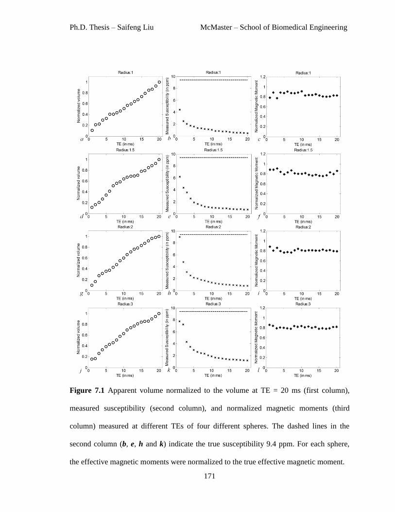
Ph.D. Thesis – Saifeng Liu McMaster – School of Biomedical Engineering
171
Figure 7.1 Apparent volume normalized to the volume at TE = 20 ms (first column),
measured susceptibility (second column), and normalized magnetic moments (third
column) measured at different TEs of four different spheres. The dashed lines in the
second column (b, e, h and k) indicate the true susceptibility 9.4 ppm. For each sphere,
the effective magnetic moments were normalized to the true effective magnetic moment.

Ph.D. Thesis – Saifeng Liu McMaster – School of Biomedical Engineering
172
Phantom experiments
A total of 14 air bubbles and 9 glass beads were examined in the phantom data. The
measured spin echo volumes of the glass beads and air bubbles are shown in Tables 7.1
and 7.2. In these two tables, the glass beads as well as air bubbles are sorted based on
their spin echo volumes, from small to large objects. The diameters of these glass beads
calculated from their spin echo volumes agree reasonably well with their physically
measured diameters, as shown in Table 7.1. Also note that, the error in volume
measurement is unreliable for spherical objects with radii less than 1.5 pixels (14.13
voxels for the volume). The error is generally larger than 20%, as shown in the
simulations. Thus, the first two smallest air bubbles were excluded from the analysis.
Fig. 7.2 shows three orthogonal views of the susceptibility map of the largest glass bead
for the shortest TE and the longest TE. Fig. 7.3 shows the susceptibility maps obtained
using the newer data processing algorithms. Compared with the former results, the
streaking artefacts are reduced and the objects are more homogeneous.

Ph.D. Thesis – Saifeng Liu McMaster – School of Biomedical Engineering
173
Table 7.1 Spin echo volume (in voxels) and the diameter (in mm) calculated from spin
echo volume for each glass bead.
Bead
Measure
1 2 3 4 5 6 7 8 9
Spin Echo Volume 35.4 37.5 38.2 39.1 96.5 103.8 113.6 516.6 912.1
Spin Echo Diameter 2.0 2.1 2.1 2.1 2.9 2.9 3.0 5.0 6.0
Actual Diameter 2.0 2.0 2.0 2.0 3.0 3.0 3.0 5.0 6.0
Table 7.2 Spin echo volume (in voxel) of the 14 air bubbles.
Bubble 1 2 3 4 5 6 7
Volume 3.3 15.1 28.7 42.2 43.9 82.8 87.7
Bubble 8 9 10 11 12 13 14
Volume 92.7 118.2 170.5 238.6 288.7 322.7 897.2

Ph.D. Thesis – Saifeng Liu McMaster – School of Biomedical Engineering
174
Figure 7.2 Axial, sagittal and coronal views of the susceptibility maps with TE=3.93ms
(a, b and c) and TE=26.61ms (d, e and f). The main field direction is in “y” direction.
Glass bead No. 9 in Table 7.1 is pointed by the white arrows. The air bubbles are pointed
by the white dashed arrows.
Figure 7.3 Axial, sagittal and coronal views of the susceptibility maps with TE=3.93ms
(a, b and c) and TE=26.61ms (d, e and f), obtained using newer data processing
algorithms.

Ph.D. Thesis – Saifeng Liu McMaster – School of Biomedical Engineering
175
Using Eq. 7.6, the measured susceptibilities can be corrected with the volume estimated
from the spin echo images. These results were shown in Table 7.3. The results obtained
using the newer algorithms were shown in Table 7.4. Using the original data processing
methods (i.e. geometry based artefact reduction together with 2D quadratic fitting for
background field removal, and truncated k-space division for susceptibility mapping), the
mean of the corrected susceptibility values of the glass beads averaged over all the TEs
was −1.82±0.17ppm, which is within the range of the measured values in the previous
study (15). The mean of the corrected susceptibility values of the air bubbles was
6.66±0.85ppm. This is to be compared to the actual susceptibility of 9.4ppm. Using the
new data processing algorithms (i.e. SHARP for background field removal, iterative
SWIM for susceptibility mapping), the corrected average susceptibility of the glass beads
was -2.12±0.15ppm, and the corrected average susceptibility of the air bubbles was
7.35±1.13ppm.
The susceptibility values estimated using the newer data processing algorithms are plotted
as a function of echo time in Fig. 7.4. As shown in Fig. 7.4.a, the absolute susceptibility
values of both the air bubbles and glass beads decreases as TE increases, due to the over-
estimated volume. And the corrected susceptibility values are almost constant over
different TEs, indicating that the product of susceptibility and the measured volume, or
the effective magnetic moment, is also constant. After correction, both the distributions of
susceptibility of air bubble and glass beads became narrower, indicating reduced
uncertainties in the susceptibility estimates, as shown in Fig. 7.4.c and 7.4.d.

Ph.D. Thesis – Saifeng Liu McMaster – School of Biomedical Engineering
176
Table 7.3 Mean measured and corrected susceptibilities (in ppm) of the glass beads and
air bubbles and different TEs.
Glass Bead Air bubble
TE/ms Measured Corrected Measured Corrected
3.93 -1.50±0.07 -1.79±0.13 3.15±1.16 6.13±0.77
9.60 -1.07±0.32 -1.76±0.13 1.70±0.61 6.44±0.90
15.27 -0.86±0.32 -1.82±0.19 1.30±0.45 6.64±0.76
20.94 -0.68±0.28 -1.82±0.18 1.07±0.36 6.88±0.77
26.61 -0.59±0.25 -1.88±0.21 0.93±0.34 7.22±0.74
Table 7.4 Mean measured and corrected susceptibilities (in ppm) of the glass beads and
air bubbles and different TEs. These results were obtained using the new data processing
algorithms.
Glass Bead Air bubble
TE/ms Measured Corrected Measured Corrected
3.93 -1.73±0.06 -2.06±0.15 3.58±1.41 7.24±1.01
9.60 -1.29±0.35 -2.13±0.15 1.87±0.68 7.40±1.16
15.27 -1.02±0.38 -2.16±0.16 1.36±0.48 7.39±1.20
20.94 -0.79±0.34 -2.10±0.14 1.08±0.37 7.35±1.21
26.61 -0.68±0.29 -2.17±0.18 0.89±0.31 7.38±1.23

Ph.D. Thesis – Saifeng Liu McMaster – School of Biomedical Engineering
177
Figure 7.4 a) Originally measured susceptibility values at different TEs for glass beads
and air bubbles. b) Corrected susceptibility values. c) Distribution of the originally
measured susceptibility values. d) Distribution of the corrected susceptibility values.
After correction using the spin echo volume, the glass beads can be clearly distinguished
from air bubbles. These results were obtained using the new data processing algorithms.
7.4 Discussion and Conclusions
The susceptibility mapping technique using the regularized Fourier based method has
certain advantages over other methods, especially in terms of time-efficiency and
simplicity. However, it suffers from problems caused by the intrinsic singularities in the
inverse of the Green's function, as well as partial volume effects which disrupt the true
0 10 20 30
-2
0
2
4
6
8
10
12
TE / ms
Su
sce
ptib
ility / p
pm
0 10 20 30
-2
0
2
4
6
8
10
12
TE / ms
Su
sce
ptib
ility / p
pm
-5 0 5 10 150
5
10
15
20
Susceptibility / ppm
Co
un
ts
Glass beads
Air bubbles
-5 0 5 10 150
10
20
30
40
50
Susceptibility / ppm
Co
un
ts
Glass beads
Air bubbles
0 5 10 15 20 25 30
-2
0
2
4
6
8
10
12
14
TE / ms
Susceptibili
ty /
ppm
Glass bead
Air bubble
a b
c d

Ph.D. Thesis – Saifeng Liu McMaster – School of Biomedical Engineering
178
phase behavior. For small objects, susceptibility quantification using the inverse method
(1) yields a significant under-estimation of the susceptibility. The increased apparent
volume at long TE can be utilized to create a larger virtual object, for which the true
volume can be more accurately measured and thus the Fourier based susceptibility
quantification gives a relatively smaller error for the magnetic moment. At this point, the
susceptibility close to the actual value can be extracted from the estimated magnetic
moment with an estimation of the true volume, either if it is known ahead of time, or it
can be estimated from a high resolution spin echo dataset.
Based on the discussions above, the error in the corrected susceptibility comes
from the estimated magnetic moment = and estimated volume (V). Through
error propagation, the error in the corrected susceptibility is given by:
√(
)
(
)
[7.9]
As can be seen from Eq. 7.9, the smaller the error in the estimated volume, the smaller the
error in the corrected susceptibility. This equation explains the error seen in the corrected
susceptibility of the air bubbles as well as glass beads.
In simulations, where the true volume is known, the remnant under-estimation in the
averaged corrected susceptibility ranges from 15% to 19%. Since there is no error in the
true volume, this error must be due to the error in the apparent volume measurement and
quantification due to the regularization process. The level of under-estimation is
related to the threshold value in the inverse of the Green’s function. A smaller threshold

Ph.D. Thesis – Saifeng Liu McMaster – School of Biomedical Engineering
179
leads to less under-estimation, but more streaking artefacts in the susceptibility maps. The
regularized Fourier based method, with threshold value of 0.1, can lead to an under-
estimation of around 13% for objects with radii larger than 3 pixels and even worse for
smaller objects (1, 6). This can be viewed as a systematic error, and can be reduced using
the k-space/image domain iterative algorithm, as shown in previous chapters.
In phantom studies, using high-pass filtered phase images and truncated k-space division
for generating susceptibility maps, the corrected susceptibility values of the air bubbles
have a maximum underestimation close to 44%, compared to the theoretical value 9.4ppm,
even after using the volume estimated from the spin echo data. This is essentially a
consequence of three factors: the error in the spin echo volume measurement, the signal
loss due to high-pass filtering, and the under-estimation of quantified using the
truncated k-space division method. To overcome the limitations related to volume
estimation, one has to go to high resolution images that can minimize volume
quantification error. However, the decreased SNR in high resolution spin echo images
may introduce additional variation/noise in the final volume results.
The accuracy in the susceptibility estimation can be further improved using more
sophisticated background field removal and susceptibility mapping methods. Using the
newer data processing algorithms, the background phase was better reduced. Particularly,
the streaking artefacts surrounding the air bubbles and glass beads were largely reduced
due to the use of geometry constrained iterative SWIM algorithm. Finally, the phase
values of the pixels inside the air bubbles and glass beads are not reliable, due to the low

Ph.D. Thesis – Saifeng Liu McMaster – School of Biomedical Engineering
180
signal inside these objects. This is solved by updating the phase values inside, using the
predicted phase, during the iterative SWIM algorithm. This helps to get a faster
convergence. All of these help to improve the accuracy in estimating the susceptibilities
of small objects with low signal inside.
There are a number of limitations to this study. Even though a forward calculation was
carried out to reduce the geometry induced field variation, remnant background field
variation still exists. To best account for it, the phase inside the spherical objects was set
to the local average phase. This also helps to reduce the large variation in susceptibility
estimate induced by Gibbs ringing and thermal noise. However, this phase correction
process is based on the assumption that the object of interest is a sphere. For non-
spherical objects, this phase correction process may lead to variations of magnetic
moment at different TEs. In addition, phase correction also creates a virtually larger
object. It is possible that the center of the created object deviates from the true center of
the original object of interest. This leads to additional errors even for spherical objects, as
seen from simulations. Thus, the phase inside the spherical object has significant effects
to this method. Theoretically, only when the center of a simulated large sphere coincides
with the original center of the sphere, and when the background phase value is 0, can we
obtain constant magnetic moment across different TEs. Hence, slight variation in object
definition from binary mask, which is used for phase substitution, can introduce
variations in magnetic moment values. This is the essential source of shape dependence of
the proposed method.

Ph.D. Thesis – Saifeng Liu McMaster – School of Biomedical Engineering
181
Although the estimated magnetic moments of the glass beads are almost a constant over
different TEs, as indicated by the corrected susceptibilities, the estimated magnetic
moments of the air bubbles are usually larger at a longer TE than at a shorter TE. This can
be understood by the fact that the air bubbles are not perfect spherical objects compared to
the glass beads. In fact, most of the air bubbles have ellipsoidal shapes, and any attempt of
phase correction inside the bubble based on the assumption of the spherical shape will
cause errors in the susceptibility measurement and thus lead to errors in the measurement
of the magnetic moments.
Generally speaking, for small objects which can be well approximated as spheres, the
theoretically expected errors in the estimated magnetic moment measurements are within
20% of the expected values and can be further reduced by adjusting the regularization
thresholds in the susceptibility mapping method. Practically, the errors might be larger
due to the limited knowledge of the true volume. While most small microbleeds can be
well approximated as spheres, the use of more accurate volume estimation methods has
the potential to reduce the error in susceptibility quantification of microbleeds.
In conclusion, we have shown that for very small structures, obtaining accurate magnetic
susceptibility values is limited by the errors in the volume estimations of these structures
and in the Fourier based method itself. Despite this inability to estimate the actual volume
of a small object accurately (whether it is an air bubble or microbleed), the estimated
magnetic moment is almost a constant over different TEs. This demonstrates that it is
possible to measure the magnetic moment at a longer TE when the apparent volume is

Ph.D. Thesis – Saifeng Liu McMaster – School of Biomedical Engineering
182
increased due to T2* dephasing. By measuring or knowing a priori the actual volume of
an object, it is possible to obtain a reasonable estimate of the susceptibility.
Acknowledgments This work is supported in part by National Institutes of Health via
grants NHLBI R01HL062983-A4 and NHLBI R21 HL 108230-A2. This work is also
supported in part by the Wayne State University Perinatal Research Initiative.

Ph.D. Thesis – Saifeng Liu McMaster – School of Biomedical Engineering
183
References
1. Haacke EM, Tang J, Neelavalli J, Cheng YC. Susceptibility mapping as a means to
visualize veins and quantify oxygen saturation. Journal of Magnetic Resonance
Imaging 2010; 32(3):663-676.
2. Liu T, Spincemaille P, de Rochefort L, Kressler B, Wang Y. Calculation of
susceptibility through multiple orientation sampling (COSMOS): A method for
conditioning the inverse problem from measured magnetic field map to susceptibility
source image in MRI. Magnetic Resonance in Medicine 2009; 61(1):196-204.
3. de Rochefort L, Brown R, Prince MR, Wang Y. Quantitative MR susceptibility
mapping using piece-wise constant regularized inversion of the magnetic field.
Magnetic Resonance in Medicine 2008; 60(4):1003-1009.
4. Schweser F, Deistung A, Lehr BW, Reichenbach JR. Quantitative imaging of intrinsic
magnetic tissue properties using MRI signal phase: An approach to in vivo brain iron
metabolism? NeuroImage 2011; 54(4):2789-2807.
5. Wharton S, Schäfer A, Bowtell R. Susceptibility mapping in the human brain using
threshold-based k-space division. Magnetic Resonance in Medicine 2010; 63(5):1292-
1304.
6. Shmueli K, de Zwart JA, van Gelderen P, Li T, Dodd SJ, Duyn JH. Magnetic
susceptibility mapping of brain tissue in vivo using MRI phase data. Magnetic
Resonance in Medicine 2009; 62(6):1510-1522.
7. Ayaz M, Boikov AS, Haacke EM, Kido DK, Kirsch WM. Imaging cerebral
microbleeds using susceptibility weighted imaging: One step toward detecting vascular
dementia. Journal of Magnetic Resonance Imaging 2010; 31(1):142-148.
8. Greenberg SM, Vernooij MW, Cordonnier C, Viswanathan A, Al-Shahi Salman R,
Warach S, Launer LJ, Van Buchem MA, Breteler MM. Cerebral microbleeds: a guide
to detection and interpretation. The Lancet Neurology 2009; 8(2):165-174.
9. Yates PA, Sirisriro R, Villemagne VL, Farquharson S, Masters CL, Rowe CC, For the
AIBL Research Group. Cerebral microhemorrhage and brain β-amyloid in aging and
Alzheimer disease. Neurology 2011; 77(1):48 -54.
10. Cheng Y-CN, Neelavalli J, Haacke EM. Limitations of calculating field distributions
and magnetic susceptibilities in MRI using a Fourier based method. Physics in
Medicine and Biology. 2009; 54(5):1169-1189.
11. McAuley G, Schrag M, Barnes S, Obenaus A, Dickson A, Holshouser B, Kirsch W.
Iron quantification of microbleeds in postmortem brain. Magnetic Resonance in
Medicine 2011; 65(6):1592-1601.
12. Liu T, Surapaneni K, Lou M, Cheng L, Spincemaille P, Wang Y. Cerebral
Microbleeds : Burden Assessment by Using Quantitative Susceptibility Mapping.
Radiology (2012); 262(1):269-78.
13. Cheng Y-C, Hsieh C-Y, Neelavalli J, Haacke EM. Quantifying effective magnetic
moments of narrow cylindrical objects in MRI. Physics in Medicine and Biology. 2009;
54(22):7025-7044.
14. Haacke EM, Brown RW, Thompson MR, Venkatesan R. Magnetic Resonance
Imaging: Physical Principles and Sequence Design. 1st ed. Wiley-Liss; 1999.

Ph.D. Thesis – Saifeng Liu McMaster – School of Biomedical Engineering
184
15. Hsieh C, Cheng Y, Tackett R, Kumar R, Lawes G, Haacke E. TH-D-304A-02:
Quantifying Magnetic Moments and Susceptibilities of Small Spherical Objects in
MRI. Medical Physics 2009; 36:2816.
16. Neelavalli J, Cheng YN, Jiang J, Haacke EM. Removing background phase variations
in susceptibility-weighted imaging using a fast, forward-field calculation. Journal of
Magnetic Resonance Imaging 2009; 29(4):937-948.
17. Jenkinson M. Fast, automated, N-dimensional phase-unwrapping algorithm. Magnetic
Resonance in Medicine 2003; 49(1):193-197.
18. Schweser F, Deistung A, Lehr BW, Reichenbach JR. Quantitative imaging of intrinsic
magnetic tissue properties using MRI signal phase: An approach to in vivo brain iron
metabolism? NeuroImage. 2011 Feb 14;54(4):2789–807.
19. Tang J, Liu S, Neelavalli J, Cheng YCN, Buch S, Haacke EM. Improving
susceptibility mapping using a threshold-based K-space/image domain iterative
reconstruction approach. Magn Reson Med. 2013 May;69(5):1396–407.
20. Tofts PS, Silver NC, Barker GJ, Gass A. Object strength-an accurate measure for
small objects that is insensitive to partial volume effects. MAGMA 2005; 18(3):162-
169.
21. Gudbjartsson, H., and Patz, S. The Rician distribution of noisy MRI data. Magnetic
Resonance in Medicine 1995; 34(6):910-914.

Ph.D. Thesis – Saifeng Liu McMaster – School of Biomedical Engineering
185
Chapter 8 Conclusions and Future
Directions
Quantitative susceptibility mapping (QSM) is a promising technique to study tissue
properties such as iron content and function such as oxygen extraction in vivo. In this
thesis, several technical advances in the QSM methodology have been made which will
accelerate the data processing and improve the accuracy of QSM.
First, the quality of QSM is largely dependent on background field removal. From the
results of simulations and in vivo data studies, the spherical mean value filtering (SMV)
based techniques are the most effective method, both in terms of the time-efficiency and
accuracy. However, the regions close to the edge of the brain are usually eroded in order
to avoid noisy pixels outside the brain. This is the main remnant problem of these SMV
based background field removal algorithms. For studies focused on the cerebral venous
oxygen saturation, the superior sagittal sinus (SSS) is of great interest. But the accuracy
of the extracted local phase information for the superior sagittal sinus is poor, since SSS
is sitting at the edge of the brain and may be partly removed by the brain extraction step.
Thus, it is critical to keep this structure using the binary brain mask and to keep the phase
at the edge of the SSS or even outside the SSS in the skull (1,2).

Ph.D. Thesis – Saifeng Liu McMaster – School of Biomedical Engineering
186
The Local Spherical Mean Value filtering (LSMV) algorithm proposed in this thesis
improves the robustness and efficiency for background field removal. It is particularly
time-efficient for processing data collected with double- or multi- echo. The main
advantage of this algorithm is avoiding global phase unwrapping and the reduction of
phase signal loss near the edges of the veins due to T2* signal decay. It can also be used
for processing of data collected with a single short TE. The local background field
removal also helps to reduce the effects of cusp artefacts/phase singularities, which are
typically caused by improper combination of multi-channel data.
Proper multi-channel phase data combination is critical for data collected using phased
array coils and parallel imaging techniques such as GRAPPA (3). Any improper
combination of the phase will lead to signal cancellation and cusp artefacts (4,5). For
regions inside the brain, the cusp artefacts can be avoided by correcting the linear
gradients and baseline differences of different channels. But for regions outside the brain,
such a simple correction may still lead to cusp artefacts (6). This is again due to the
difference in the phase references of different channels, , which contains both the coil-
sensitivity induced phase components and the conductivity induced phase components.
Thus, the ideal phase combination should have the removed from each channel before
combining all the channels’ data. This can be done by using either a reference scan or
reference echo (6). In the former method, usually the reference scan is performed using
coils with relatively uniform sensitivity profile. In the latter method, the TE of the
reference echo could be chosen such that it equals half of the TE of the main scan. Then
can be calculated using these two echoes using complex division (without phase

Ph.D. Thesis – Saifeng Liu McMaster – School of Biomedical Engineering
187
unwrapping). Removing these spatially varying effects will then lead to an improved
QSM reconstruction.
Second, QSM is essentially an ill-posed inverse problem. For solving the inverse problem,
the main difference in currently available algorithms is related to the handling of the
gradients/edges in the susceptibility maps. In order to suppress false gradients caused by
the streaking artefacts, the gradients estimated from magnitude images and phase images
or a combination of both are usually used as a priori information (7,8). Care should be
taken when imposing these a priori constraints. While a false edge detected from
magnitude or phase images will reduce the effectiveness in removing the streaking
artefacts in the susceptibility maps, a missed edge will lead to over-smoothing of the
susceptibility maps. For clinical studies, the processing time for these methods is also of
concern, especially when large numbers of datasets with large matrix size are involved.
The k-space/image domain iterative algorithm (iterative SWIM) is a promising method,
precisely because of its proper preserving of the edge information in the susceptibility
maps and its time-efficiency. As validated using simulated data and in vivo data, this
iterative SWIM algorithm is particularly effective for studies focused on measuring
venous oxygen saturation.
An improved version of the iterative SWIM algorithm, which utilizes the geometries of
the structures found in the susceptibility maps for solving the inverse problem, is
demonstrated in this thesis. Instead of using the geometries of the structures with high
susceptibilities, e.g., veins, as in the original iterative SWIM algorithm (9), in the

Ph.D. Thesis – Saifeng Liu McMaster – School of Biomedical Engineering
188
improved version proposed in this thesis, both the geometries of the veins and grey matter
structures (with relatively high susceptibilities) were extracted and utilized in solving the
inverse problem. This improves the accuracy of susceptibility estimation of both the veins
and the grey matter structures.
The accuracy of QSM is also dependent on the estimation of the volume, especially for
small objects (10). Longer TE gives higher phase values and potentially higher phase
SNR, but it also leads to more T2* signal decay and larger apparent volume of the object.
Any error in estimating the volume of the object will lead to error in estimating the
susceptibility of that object (10). On the other hand, the effective magnetic moment can
be used as surrogate to reflect the changes of the object of interest (10-12).
Furthermore, the susceptibility maps can also be combined with the magnitude images to
produce tSWI images (13,14). This helps to remove the orientation dependence of
conventional SWI data. These tSWI images provide improved delineation of the
geometries of veins and microbleeds and tSWI data processing can be easily incorporated
with the current SWI data processing scheme. Thus tSWI has great potential in studies of
traumatic brain injury (TBI) (13).
There are also a few limitations in the techniques presented in this thesis. First, all of the
techniques are for the data collected with single orientation. Orientation dependence of
the susceptibility values of the white matter structures has been reported in former studies,
and has been attributed to the myelin sheath surrounding the axons in the white matter
(15–18). This requires more sophisticated models to describe the relation between field

Ph.D. Thesis – Saifeng Liu McMaster – School of Biomedical Engineering
189
variation and susceptibility distribution (19–21). In addition to the susceptibility
anisotropy, nonlinear phase evolution was also observed and can be modeled using multi
water compartments (17). Both the orientation dependence and nonlinear phase evolution
are neglected in this thesis, since this thesis is focused on the deep grey matter structures
and veins (18). Second, the method of improving the accuracy of susceptibility
quantification using volume constraint was only demonstrated with a phantom, but
without any in vivo data. The main application of this method is quantification of cerebral
microbleeds or calcifications. For in vivo data, an estimate of the true volume of the
microbleeds from the spin echo data may not be available. If multi-echo data were
collected, it is possible to get an estimate of the true volume at TE=0 through
extrapolation using the measured apparent volumes at different TEs. Otherwise, the
effective magnetic moment could be used to study the longitudinal changes of the
microbleeds or calcifications (12).
Future directions include the following aspects. First, the performance of the iterative
SWIM algorithm for solving the ill-posed inverse problem in susceptibility mapping
could be improved. The effectiveness of the iterative SWIM algorithm relies on proper
extraction of the geometries of different structures of interest. Currently, the geometries
are extracted purely from susceptibility maps. The accuracy of the extracted geometries
could be potentially improved by incorporating the geometries found in the magnitude
and phase images (8). Second, the lost phase information near the edge of the brain, due
to erosion of the background field removal algorithm, should be recovered as much as
possible. This can be achieved by preserving the signal outside the brain. Previous studies

Ph.D. Thesis – Saifeng Liu McMaster – School of Biomedical Engineering
190
have already shown that it is possible to keep the phase in the skull region (22). This
provides more accurate boundary conditions for background field removal and thus
reduces the error of background field removal near the edges of the brain. Third, the
accuracy of susceptibility quantification could be further improved. Particularly, the
quantification of the susceptibility of veins is usually affected by partial volume effects,
especially for small veins. Future studies should aim to model and compensate for the
partial volume effects. Other future directions include: compensation for the signal loss
caused by homodyne high-pass filtering, in a way similar to the deconvolution step in
SHARP; incorporation of partial volume effects in the magnitude and phase images of the
3D brain model.
In conclusion, quantitative susceptibility mapping is a promising technique which has
many potential applications. It can be applied to most of the applications found by
susceptibility weighted imaging (5,23). It is also finding newer applications, given its
ability to quantify the source of the phase information and its independence of echo time
or orientation, such as tracking and quantifying iron labeled stem cells (24). The accuracy
of QSM is dependent on both the imaging acquisition and image post-processing. This
thesis has focused on two core steps of QSM post-processing: background field removal
and solving the inverse problem. While a new algorithm has been proposed for
background field removal, an improved method for solving the inverse problem has also
been demonstrated. Both of them contribute to a more sophisticated data processing
scheme for quantitative susceptibility mapping with improved effectiveness and accuracy.

Ph.D. Thesis – Saifeng Liu McMaster – School of Biomedical Engineering
191
References
1. Li L, Leigh JS. High-precision mapping of the magnetic field utilizing the harmonic
function mean value property. J. Magn. Reson. 1997 2001;148:442–8.
2. Zhou D, Liu T, Spincemaille P, Wang Y. Background field removal by solving the
Laplacian boundary value problem. NMR Biomed. 2014;
3. Griswold MA, Jakob PM, Heidemann RM, Nittka M, Jellus V, Wang J, et al.
Generalized autocalibrating partially parallel acquisitions (GRAPPA). Magn. Reson.
Med. 2002;47:1202–10.
4. Hammond KE, Lupo JM, Xu D, Metcalf M, Kelley DAC, Pelletier D, et al.
Development of a robust method for generating 7.0 T multichannel phase images of
the brain with application to normal volunteers and patients with neurological
diseases. NeuroImage 2008;39:1682–92.
5. Haacke EM, Reichenbach JR, editors. Susceptibility Weighted Imaging in MRI:
Basic Concepts and Clinical Applications. 1st ed. Wiley-Blackwell; 2011.
6. Robinson S, Grabner G, Witoszynskyj S, Trattnig S. Combining phase images from
multi-channel RF coils using 3D phase offset maps derived from a dual-echo scan.
Magn. Reson. Med. 2011;65:1638–48.
7. Liu J, Liu T, de Rochefort L, Ledoux J, Khalidov I, Chen W, et al. Morphology
enabled dipole inversion for quantitative susceptibility mapping using structural
consistency between the magnitude image and the susceptibility map. NeuroImage
2012;59:2560–8.
8. Schweser F, Sommer K, Deistung A, Reichenbach JR. Quantitative susceptibility
mapping for investigating subtle susceptibility variations in the human brain.
NeuroImage 2012;62:2083–100.
9. Tang J, Liu S, Neelavalli J, Cheng YCN, Buch S, Haacke EM. Improving
susceptibility mapping using a threshold-based K-space/image domain iterative
reconstruction approach. Magn. Reson. Med. 2013;69:1396–407.
10. Liu S, Neelavalli J, Cheng Y-CN, Tang J, Mark Haacke E. Quantitative
susceptibility mapping of small objects using volume constraints. Magn. Reson.
Med. 2013;69:716–23.
11. Schweser F, Deistung A, Lehr BW, Reichenbach JR. Differentiation between
diamagnetic and paramagnetic cerebral lesions based on magnetic susceptibility
mapping. Med. Phys. 2010;37:5165.

Ph.D. Thesis – Saifeng Liu McMaster – School of Biomedical Engineering
192
12. Liu T, Surapaneni K, Lou M, Cheng L, Spincemaille P, Wang Y. Cerebral
microbleeds: burden assessment by using quantitative susceptibility mapping.
Radiology 2012;262:269–78.
13. Liu S, Mok K, Neelavalli J, Cheng YCN, Tang J, Ye Y, et al. Improved MR
Venography Using Quantitative Susceptibility-Weighted Imaging. J. Magn. Reson.
Imaging 2013;
14. Gho S-M, Liu C, Li W, Jang U, Kim EY, Hwang D, et al. Susceptibility map-
weighted imaging (SMWI) for neuroimaging. Magn. Reson. Med. 2013;
15. Liu C, Li W, Johnson GA, Wu B. High-field (9.4 T) MRI of brain dysmyelination
by quantitative mapping of magnetic susceptibility. NeuroImage 2011;56:930–8.
16. Li X, Vikram DS, Lim IAL, Jones CK, Farrell JAD, van Zijl PCM. Mapping
magnetic susceptibility anisotropies of white matter in vivo in the human brain at 7
T. NeuroImage 2012;62:314–30.
17. Wharton S, Bowtell R. Fiber orientation-dependent white matter contrast in gradient
echo MRI. Proc. Natl. Acad. Sci. U. S. A. 2012;109:18559–64.
18. Rudko DA, Klassen LM, de Chickera SN, Gati JS, Dekaban GA, Menon RS.
Origins of orientation dependence in gray and white matter. Proc. Natl. Acad. Sci. U.
S. A. 2014;111:E159–167.
19. He X, Yablonskiy DA. Biophysical mechanisms of phase contrast in gradient echo
MRI. Proc. Natl. Acad. Sci. U. S. A. 2009;106:13558–63.
20. Liu C. Susceptibility tensor imaging. Magn. Reson. Med. 2010;63:1471–7.
21. Luo J, He X, Yablonskiy DA. Magnetic susceptibility induced white matter MR
signal frequency shifts-experimental comparison between Lorentzian sphere and
generalized Lorentzian approaches. Magn. Reson. Med. 2013;
22. Buch S, Liu S, Cheng Y, Haacke E. Susceptibility Mapping of the Sinuses in the
Brain by Preserving Phase Information in the Skull Using Short Echo Times. Proc.
21st Annu. Meet. ISMRM Salt Lake City Utah USA 2013;:2483.
23. Mittal S, Wu Z, Neelavalli J, Haacke EM. Susceptibility-Weighted Imaging:
Technical Aspects and Clinical Applications, Part 2. Am. J. Neuroradiol.
2009;30:232–52.
24. Ruggiero A, Guenoun J, Smit H, Doeswijk GN, Klein S, Krestin GP, et al. In vivo
MRI mapping of iron oxide-labeled stem cells transplanted in the heart. Contrast
Media Mol. Imaging 2013;8:487–94.