Teams as Superstars: Effort and Risk Taking in

Rank-Order Tournaments for Women and Men

by

Mario Lackner

Working Paper No. 1613

December 2016

DDEEPPAARRTTMMEENNTT OOFF EECCOONNOOMMIICCSS

JJOOHHAANNNNEESS KKEEPPLLEERR UUNNIIVVEERRSSIITTYY OOFF

LLIINNZZ

Johannes Kepler University of Linz Department of Economics

Altenberger Strasse 69 A-4040 Linz - Auhof, Austria

www.econ.jku.at

mario.lackner@jku.at

Teams as Superstars: Effort and Risk Taking in

Rank-Order Tournaments for Women and Men

Mario Lackner∗

Department of Economics, JKU Linz

December 5, 2016

Abstract

This article analyzes top-level basketball competitions and measures the effectof superstar presence on effort provision in rank-order tournaments. I extend theprevious literature to team competitions for male and female teams, as well asdifferent institutional settings over a long period of time. In addition, I analyzerisk-taking behavior in the context of superstar effects. The results of the empiricalanalysis suggests that the level of superstar dominance is crucial for the observedeffects. While there is an significant and sizeable effort reducing superstar effect,less (little) dominance by the superstar seems to be result in a positive peer effects.

JEL Classification: D70, M51, J01

Keywords : superstar effects, rank-order tournaments, incentives, effort, risk-taking

∗Address for correspondence: Johannes Kepler University of Linz, Department of Economics,Altenbergerstr. 69, 4040 Linz, Austria. Phone:+43 70 2468 7390, Fax: +43 70 2468 7390, email:mario.lackner@jku.at. I am grateful for funding by the Austrian National Bank, project number 16242,project website. Helpful comments from Brad Humphreys and participants at the 2014 European SportsEconomics Conference are gratefully acknowledged. The usual disclaimer applies.

1 Introduction

Economic decision making regularly involves strategic interactions within groups of het-

erogenous contestants. For example, workers face decision environments (e.g. promotion

tournaments) with incentive systems that involve strategic decisions about effort provision

or risk-taking. The reactions of contestants to incentives, contest design and contestants’

heterogeneity has been a central focus of the theoretical literature (Lazear and Rosen,

1981; Baik, 1994; Stracke et al., 2015). In the majority of contests competitors are het-

erogenous in terms of ability or status. In the extreme case one contestant stands out

and represents a superstar among relatively inferior contestants. In a seminal article, the

term superstar was defined by Rosen (1981, p. 845) as

[...] relatively small numbers of people earn enormous amounts of money and

dominate the activities in which they engage [...]

In general, superstars are usually interpreted as single competitors who have a dispro-

portionately larger chance to win a contest or tournament due to their relatively large

ability. A substantial part of the literature on the superstar phenomenon has dealt with

the share of total wages that are allocated top superstars (Lucifora and Simmons, 2003)

or the general environment where superstars are usually observed (Fort and Quirk, 1995).

Malmendier and Tate (2009) analyze the performance of firms who are led by superstar

CEOs and find that those firms exhibit lower performance levels after the CEO achieved

superstar status. A particular interest in sports economics is the effect of superstar pres-

ence on fan or media attendance (Hausman and Leonard, 1997; Krueger, 2005; Brandes

et al., 2008; Kuethe and Motamed, 2010).

Sporting competitions represent an ideal environment to empirically analyze superstar

effects on decision making of individual competitors and teams. Data on financial incen-

tives (i.e. the prize structure), wages as well as very good measures for relative ability

are frequently available. Additionally, sports contest feature a multitude of competitive

settings with clearly defined incentive structures and prizes (Szymanski, 2003).

In this article I extend the previous empirical literature on the superstar effect in sports

competitions (e.g. Brown (2011) or Hill (2014)). Along the definition of Rosen (1981),

I define a superstar as a team of professional basketball players competing in a dynamic

tournament of multiple stages. As shown by Kocher and Sutter (2005) or Charness and

Sutter (2012), it is highly plausible that teams or groups of individuals are even better

(i.e. more efficient) decision makers than individuals. In particular, I will analyze if teams

who are in direct competition with a superstar-team in a rank-order tournament will exert

2

more or less effort than without the superstar. In a second step, I will shift the focus to

risk taking behavior.

Superstar effects in group-wise rank-order competitions are relevant for a wide array of

settings. Promotion tournaments in firms are often designed similar to a round-robin

rank-order tournament. The ultimate goal is to find the job candidate with the high-

est ability while maximizing total effort of all contestants throughout the competition.

Superstar effects are also relevant when incentive payments are introduced and enforced

according to a performance ranking. Another obvious example are patent races or com-

petitive innovation processes (Boudreau, Lacetera and Lakhani, 2011). A similar setting

to teams competing in sports contests is found in politics. Electoral contests are more

often observed between parties or interest groups rather than individual candidates. More

general, any competition among firms could be influenced by the vast superiority of one

firm, which could lead to undesirable and inefficient outcomes (Chan, Li and Pierce, 2014).

Undeniably, the designers of sports contests have to consider superstar effects in order to

maintain a certain level of overall competitiveness (Jane, 2014).

Since Basketball was included in the Olympic Games, the teams from the United States

were highly successful. During the games from 1936 (Berlin) to 2012 (London) the US

Men Team has won a total of 130 games with only 5 losses (3,7%). Women’s Basketball

was a later addition to the Olympic program in 1976 (Montreal), but the US team had

similar success than their male counterpart. Up to the most resent games in 2012 the

US Women’s team has won 58 games to go along with 3 lost games (4.2%). With the

exception of the 1980 games in Moscow1 it was a highly rational expectation to expect the

US basketball teams to win every single match as well as the overall Olympic tournament.

Consequently, I will identify the male and female US basketball team as a superstar.

2 Related literature

Since the pioneering work by Lazear and Rosen (1981) and Rosen (1986), heterogeneity

among contestants was one of the focuses of the literature on performance and effort

decisions in tournaments. Recent theoretical as well as empirical contributions by Sunde

(2009), Stracke and Sunde (2014), Stracke et al. (2015) and Brown and Minor (2014) show

that current (as well as future) heterogeneity influences effort provision of contestants in

dynamic elimination contests. Berger and Nieken (2014) as well as Deutscher et al. (2013)

1The US–along with other nations–boycotted the 1980 Olympic Games due to political tensions atthe heights of the cold war.

3

use data from round-robin tournaments to measure the effect of contestant heterogeneity

on effort in rank-order contests.

A specific and very pronounced form of heterogeneity in competitions is observed in the

presence of a superstar. The consequences of such superstar presence are a well described

and vividly discussed phenomenon in sports (Jane, 2014). Few empirical contributions,

however, focus on the causal effect of superstar presence in competitions on effort provision

of contestants. In a seminal paper Brown (2011) shows that the presence of a superstar

has negative effects on the performance of the other contestants in golf tournaments. The

presence of Tiger Woods as the dominating player yields lower overall performance levels

of all other players in professional golf contests. This decline in overall performance is

interpreted as a negative superstar effect on performance of Wood’s competitors. This

detrimental effect on effort provision was smaller in competitions when Woods was ex-

periencing a span of lower productivity, indicating that the different degrees of superstar

dominance lead to different shifts in competitors’ performance.

Using a three heterogenous contestant model, Brown (2011) shows that effort decreases as

heterogeneity of contestants increases. The more able the single superstar in the competi-

tion is relatively to the other contestants, the lower will be effort of other (non-superstar)

competitors. An important factor is the existence of a second prize, with the superstar

effect being more pronounced as the share of the total purse that is going to the winner.2

Jane (2014) analyze data from swimming contests and find no detrimental effect of su-

perstar presence, but rather a positive peer effect. The performance levels of heats with

a potentially dominant swimmer increase compared to heats without such a superstar

swimmer. Hill (2012), Emerson and Hill (2014) as well as Hill (2014) presents a similar

result for 100 meter sprinters a top-level competitions, confirming that the negative effect

of superstar presence is not a unanimous empirical result. This contrary finding could

potentially be due to the fact that no clear superstar is identified in the analyzed athletic

competitions.

This article expands the previous literature on the superstar effects in round-robin tour-

naments to the analysis of team behavior and compares different levels of superstar dom-

inance. The focus will be on effort and risk-taking. In addition, I will establish a causal

effect by using an exogenous rule change and measure how it changed potential superstar

effects on effort and risk-taking.

2While my empirical analysis cannot take (monetary) prizes into account, it is not problematic, asthe only (observed) reward or prize available in round-robin stages of basketball tournaments is theadvancement to the next level of the competition.

4

3 Data and Institutional Background

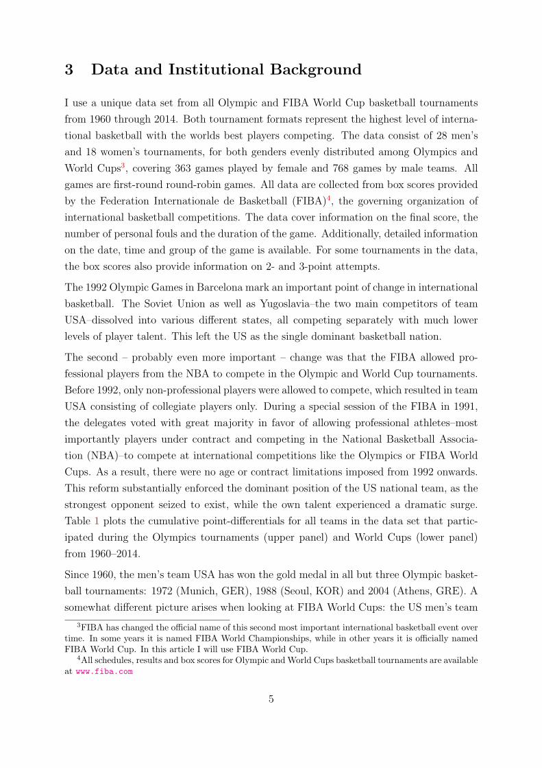
I use a unique data set from all Olympic and FIBA World Cup basketball tournaments

from 1960 through 2014. Both tournament formats represent the highest level of interna-

tional basketball with the worlds best players competing. The data consist of 28 men’s

and 18 women’s tournaments, for both genders evenly distributed among Olympics and

World Cups3, covering 363 games played by female and 768 games by male teams. All

games are first-round round-robin games. All data are collected from box scores provided

by the Federation Internationale de Basketball (FIBA)4, the governing organization of

international basketball competitions. The data cover information on the final score, the

number of personal fouls and the duration of the game. Additionally, detailed information

on the date, time and group of the game is available. For some tournaments in the data,

the box scores also provide information on 2- and 3-point attempts.

The 1992 Olympic Games in Barcelona mark an important point of change in international

basketball. The Soviet Union as well as Yugoslavia–the two main competitors of team

USA–dissolved into various different states, all competing separately with much lower

levels of player talent. This left the US as the single dominant basketball nation.

The second – probably even more important – change was that the FIBA allowed pro-

fessional players from the NBA to compete in the Olympic and World Cup tournaments.

Before 1992, only non-professional players were allowed to compete, which resulted in team

USA consisting of collegiate players only. During a special session of the FIBA in 1991,

the delegates voted with great majority in favor of allowing professional athletes–most

importantly players under contract and competing in the National Basketball Associa-

tion (NBA)–to compete at international competitions like the Olympics or FIBA World

Cups. As a result, there were no age or contract limitations imposed from 1992 onwards.

This reform substantially enforced the dominant position of the US national team, as the

strongest opponent seized to exist, while the own talent experienced a dramatic surge.

Table 1 plots the cumulative point-differentials for all teams in the data set that partic-

ipated during the Olympics tournaments (upper panel) and World Cups (lower panel)

from 1960–2014.

Since 1960, the men’s team USA has won the gold medal in all but three Olympic basket-

ball tournaments: 1972 (Munich, GER), 1988 (Seoul, KOR) and 2004 (Athens, GRE). A

somewhat different picture arises when looking at FIBA World Cups: the US men’s team

3FIBA has changed the official name of this second most important international basketball event overtime. In some years it is named FIBA World Championships, while in other years it is officially namedFIBA World Cup. In this article I will use FIBA World Cup.

4All schedules, results and box scores for Olympic andWorld Cups basketball tournaments are availableat www.fiba.com

5

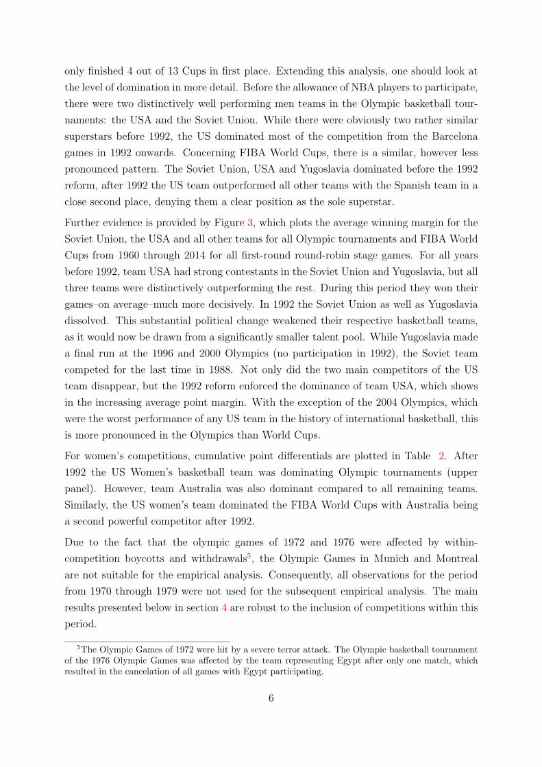
only finished 4 out of 13 Cups in first place. Extending this analysis, one should look at

the level of domination in more detail. Before the allowance of NBA players to participate,

there were two distinctively well performing men teams in the Olympic basketball tour-

naments: the USA and the Soviet Union. While there were obviously two rather similar

superstars before 1992, the US dominated most of the competition from the Barcelona

games in 1992 onwards. Concerning FIBA World Cups, there is a similar, however less

pronounced pattern. The Soviet Union, USA and Yugoslavia dominated before the 1992

reform, after 1992 the US team outperformed all other teams with the Spanish team in a

close second place, denying them a clear position as the sole superstar.

Further evidence is provided by Figure 3, which plots the average winning margin for the

Soviet Union, the USA and all other teams for all Olympic tournaments and FIBA World

Cups from 1960 through 2014 for all first-round round-robin stage games. For all years

before 1992, team USA had strong contestants in the Soviet Union and Yugoslavia, but all

three teams were distinctively outperforming the rest. During this period they won their

games–on average–much more decisively. In 1992 the Soviet Union as well as Yugoslavia

dissolved. This substantial political change weakened their respective basketball teams,

as it would now be drawn from a significantly smaller talent pool. While Yugoslavia made

a final run at the 1996 and 2000 Olympics (no participation in 1992), the Soviet team

competed for the last time in 1988. Not only did the two main competitors of the US

team disappear, but the 1992 reform enforced the dominance of team USA, which shows

in the increasing average point margin. With the exception of the 2004 Olympics, which

were the worst performance of any US team in the history of international basketball, this

is more pronounced in the Olympics than World Cups.

For women’s competitions, cumulative point differentials are plotted in Table 2. After

1992 the US Women’s basketball team was dominating Olympic tournaments (upper

panel). However, team Australia was also dominant compared to all remaining teams.

Similarly, the US women’s team dominated the FIBA World Cups with Australia being

a second powerful competitor after 1992.

Due to the fact that the olympic games of 1972 and 1976 were affected by within-

competition boycotts and withdrawals5, the Olympic Games in Munich and Montreal

are not suitable for the empirical analysis. Consequently, all observations for the period

from 1970 through 1979 were not used for the subsequent empirical analysis. The main

results presented below in section 4 are robust to the inclusion of competitions within this

period.

5The Olympic Games of 1972 were hit by a severe terror attack. The Olympic basketball tournamentof the 1976 Olympic Games was affected by the team representing Egypt after only one match, whichresulted in the cancelation of all games with Egypt participating.

6

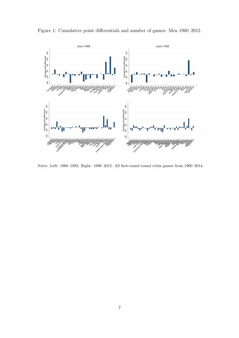
Figure 1: Cumulative point differentials and number of games: Men 1960–2012.

−6

0−

20

20

60

10

01

40

Ave

rag

e p

oin

t d

iffe

ren

tia

l

Austra

lia

Brazil

Bulga

riaCAR

Can

ada

China

Cub

a

Cze

chos

lova

kia

Egypt

Finland

Franc

e

Ger

man

y

Hun

garyIta

ly

Japa

n

Korea

Mex

ico

Mor

occo

Panam

aPer

u

Philip

pine

s

Polan

d

Puerto

Rico

Seneg

al

Soviet U

nion

SpainUSA

Uru

guay

Yugos

lavia

year>1988

−6

0−

20

20

60

10

01

40

Ave

rag

e p

oin

t d

iffe

ren

tia

l

Angola

Argen

tina

Austra

lia

BrazilCIS

Can

ada

China

Cro

atia

Franc

e

Ger

man

y

Gre

at B

ritain

Gre

eceIra

nIta

ly

Korea

Lith

uania

New

Zea

land

Niger

ia

Puerto

Rico

Rus

sia

Serbia

& Mon

t.

Spain

TunisiaUSA

Venez

uela

Yugos

lavia

year<1992−

60

−2

02

06

01

00

14

0A

ve

rag

e p

oin

t d

iffe

ren

tia

l

Angola

Argen

tina

Austra

lia

Brazil

CAR

Can

ada

China

Cot

e D’Iv

oire

Cub

a

Cze

chos

lova

kia

Dom

inican

Rep

ublic

Egypt

Franc

e

Ger

man

y

Gre

ece

Isra

elIta

ly

Japa

n

Korea

Malay

sia

Mex

ico

Net

herla

nds

New

Zea

land

Panam

a

Parag

uayPer

u

Philip

pine

s

Polan

d

Puerto

Rico

Seneg

al

Soviet U

nion

SpainUSA

Unite

d Ara

b Rep

ublic

Uru

guay

Venez

uela

Yugos

lavia

−6

0−

20

20

60

10

01

40

Ave

rag

e p

oin

t d

iffe

ren

tia

l

Alger

ia

Angola

Argen

tina

Austra

lia

Brazil

Can

ada

China

Cot

e D’Iv

oire

Cro

atia

Cub

a

Dom

inican

Rep

ublic

Egypt

Finland

Franc

e

Ger

man

y

Gre

eceIra

nIta

ly

Japa

n

Jord

an

Korea

Leba

non

Lith

uania

Mex

ico

New

Zea

land

Niger

ia

Panam

a

Philip

pine

s

Puerto

Rico

Qat

ar

Rus

sia

Seneg

al

Serbia

Serbia

& Mon

t.

Slove

nia

Spain

Tunisia

Turke

yUSA

Ukr

aine

Venez

uela

Yugos

lavia

Notes: Left: 1960–1992. Right: 1996–2012. All first-round round robin games from 1960–2014.

7

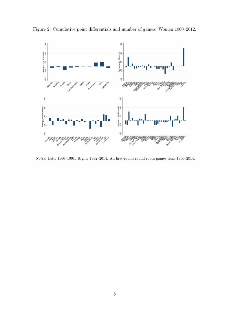
Figure 2: Cumulative point differentials and number of games: Women 1960–2012.

−6

0−

20

20

60

10

0A

ve

rag

e p

oin

t d

iffe

ren

tia

l

Austra

lia

Bulga

ria

Can

ada

China

Cze

chos

lova

kia

Japa

n

Korea

Soviet U

nion

USA

Yugos

lavia

−6

0−

20

20

60

10

0A

ve

rag

e p

oin

t d

iffe

ren

tia

l

Angola

Austra

lia

Belar

us

Brazil

Can

ada

China

Cro

atia

Cub

a

Cze

ch R

epub

lic

Cze

chos

lova

kiaDRC

Franc

e

Gre

at B

ritain

Gre

eceIta

ly

Japa

n

Korea

LatviaM

ali

New

Zea

land

Niger

ia

Polan

d

Rus

sia

Seneg

al

Slova

k Rep

ublic

Soviet U

nion

Spain

Turke

yUSA

Ukr

aine

−6

0−

20

20

60

10

0A

ve

rag

e p

oin

t d

iffe

ren

tia

l

Austra

lia

Bolivia

Brazil

Bulga

ria

Can

ada

China

Chine

se T

aipe

i

Cub

a

Cze

chos

lova

kiaDRC

Franc

e

Hun

gary

Italy

Japa

n

Korea

Malay

sia

Net

herla

ndsPer

u

Polan

d

Seneg

al

Soviet U

nion

USA

Yugos

lavia

−6

0−

20

20

60

10

0A

ve

rag

e p

oin

t d

iffe

ren

tia

l

Angola

Argen

tina

Austra

lia

Belar

us

Brazil

Can

ada

China

Chine

se T

aipe

i

Cub

a

Cze

ch R

epub

licDRC

Franc

e

Ger

man

y

Gre

ece

Hun

garyIta

ly

Japa

n

Kenya

Korea

Lith

uaniaM

ali

Moz

ambiqu

e

New

Zea

land

Niger

ia

Polan

d

Rus

sia

Seneg

al

Serbia

Slova

k Rep

ublic

Spain

Tunisia

Turke

yUSA

Yugos

lavia

Notes: Left: 1960–1991. Right: 1992–2014. All first-round round robin games from 1960–2014.

8

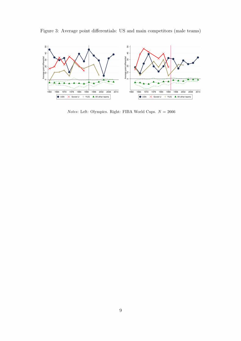
Figure 3: Average point differentials: US and main competitors (male teams)

010

20

30

40

50

Avera

ge p

oin

t diffe

rential

1960 1966 1972 1978 1984 1990 1996 2002 2008 2014

USA Soviet U YUG All other teams

010

20

30

40

50

Avera

ge p

oin

t diffe

rential

1960 1966 1972 1978 1984 1990 1996 2002 2008 2014

USA Soviet U YUG All other teams

Notes: Left: Olympics. Right: FIBA World Cups. N = 2666

9

4 Empirical Approach and Results

The empirical literature on the influence of incentives in competitive settings on effort

has proposed several proxies for effort in sports competitions. Berger and Nieken (2014)

analyze effort provision in round-robin tournaments and use the number of two-minute

penalties in handball (a direct consequence of fouls or rule infractions) as a proxy for

effort. A similar approach is chosen by Nieken and Stegh (2010), who use two-minute

penalties in hockey to proxy effort provision. Deutscher et al. (2013) make the distinction

between positive and destructive efforts by analyzing fouls and fair tackles in football

separately. An increase of positive as well as negative effort (sabotage) indicates an

increase in competition intensity as well as effort. Consequently, fouls should be a valid

proxy for individual and team effort in sports contests. In order to measure effort provision

of basketball teams, I follow the approach of previous studies on efforts in basketball

contests who identify personal fouls (or penalties) as a suitable proxy for effort. In a

closely related paper, Lackner, Stracke, Sunde and Winter-Ebmer (2015) analyze the effect

of heterogeneity multi-round pairwise elimination tournaments in professional basketball.

They use the number of fouls as a proxy for effort, arguing that a higher number of fouls

should approximate a higher intensity of the game, which should be correlated with higher

effort. In order to account for different styles of play as well as ability of basketball teams,

they use the deviation of long-term foul behavior. Data on Olympic and World Cup

basketball tournaments, however, do not provide information on long-term behavior of

teams before the observed tournaments. Consequently, I will use a fixed-effects approach

to account for unobserved ability and playing styles.

Previous studies on superstar effects on risk-taking use risky types of golf shots (Brown,

2011) or the probability of a false start in swimming legs (Jane, 2014) as identifiers for

risky strategies. Risk-taking in the context of basketball, however, is commonly measured

by the ratio of three point attempts of all attempts. This measure of risk taking is

similar to the one employed in Grund et al. (2013), who analyze the effect of intermediate

score differentials on risk taking behavior of NBA teams in round-robin and elimination

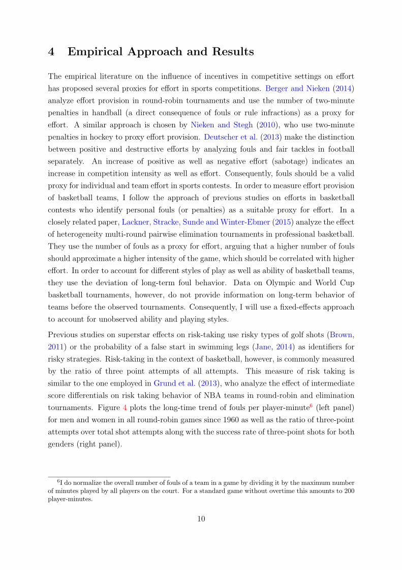
tournaments. Figure 4 plots the long-time trend of fouls per player-minute6 (left panel)

for men and women in all round-robin games since 1960 as well as the ratio of three-point

attempts over total shot attempts along with the success rate of three-point shots for both

genders (right panel).

6I do normalize the overall number of fouls of a team in a game by dividing it by the maximum numberof minutes played by all players on the court. For a standard game without overtime this amounts to 200player-minutes.

10

Figure 4: Trend of fouls per minute and three-point attempts and success: men andwomen

.08

.1.1

2.1

4.1

6A

vera

ge n

um

ber

of fo

uls

/min

1960 1966 1972 1978 1984 1990 1996 2002 2008 2014

men women

.2.3

.4.5

.6.7

Ratio 3

−poin

t/2−

poin

t attem

pts

1960 1966 1972 1978 1984 1990 1996 2002 2008 2014

attempts: men attempts: women

success: men success: women

Notes: Evolution of effort an risk-taking measure over time. Top: personal fouls per player-minute.Bottom: Percent three-point shots of all shots and success rate. Only first-round round-robin games ofOlympic and FIBA World Cup basketball tournaments were included. Only games without US partici-pation included, N = 2262

11

While the US national teams have won the majority of Olympic gold medals as well as

World Cups in the last 60 years, the 1992 reform by FIBA marks a clear shift of power

towards the men’s team USA, which was henceforth frequently called “dream team”. In

the early 90s, the vast majority of NBA players were of US nationality with only few

international players on NBA rosters (Yang and Lin, 2012). The US team superstar effect,

however, might have been mediated somewhat over time, as the number of the number of

international NBA players has steadily increased. At the same time, the quality of other

leagues has improved as a consequence of the ‘globalization’ of basketball.

All Olympic and World Cup basketball tournaments were held in several stages including

round-robin an stage-wise elimination contests. Since 1960, the tournament mode has

changed only slightly. All tournaments consist of a first round-robin stage with parallel

competition in two groups. The only exception were the 1960 (Rome) games with four

parallel groups in the first stage. Men’s World Cup tournaments are similar, with an

initial round-robin stage of 3 groups until 1982 and later on 4 parallel groups. Out of these

group stages, multiple teams advance into the following stages, which are mostly stage-

wise elimination tournaments. Only some tournaments also featured a second round-robin

stage.

In round-robin basketball competitions, it is obvious that all teams who are seeded into

the same group as the US team will be strongly affected by a possible superstar effect.7

The probability of each team–seeded into the same group as the US team–to qualify for

the next round (regardless if elimination mode or second round-robin phase) is lower

compared to teams in the other group(s). In addition to this current heterogeneity effect,

there is also a dynamic forward-looking effect. The next opponent(s) for such a team will

be stronger, as the final ranking–which is influencing the seeding for the next round–will

be lower due to the presence of team USA. Consequently, the first prize (i.e. winning the

group) and second prize (qualifying for the next tournament stage behind the US team)

are deflated through superstar presence. As a result, FIBA’s 1991 decision to allow NBA

players to participate in international competitions will affect teams competing in the

same group as the US team from 1992 onwards.

Comparing success of the US national team at Olympic Games and FIFA World Cups,

one can conclude that the US dominance was greater in the Olympics. This is surprising,

as the level of competition at the Olympics typically is higher as fewer (and on average

better) teams are competing. One potential reason for the less dominant US team is the

7Unfortunately there was no available information on seeding in both Olympics and World Cup com-petitions. However, the few tournaments where seeding information was available confirmed that themain objective of the seeding procedure was to distribute teams equally over all groups regarding theiroverall team ability. This ensures that–on average–all groups are equally talented, except that there isthe US team seeded into one of them.

12

lower reputation of winning the World Cup compared to winning Olympic gold. Brown

(2011) shows that the negative superstar effect is less pronounced when the superstar is

expected to be less dominant, i.e. when his probability to win the tournament is smaller.

This is reflected in the lower two panels of Figure 1: USA teams were the dominant teams

before and after 1991 in men’s FIBAWorld Cups. However, in contrast to the development

at the Olympics, there was at least one strong competitor after 1992 to be found in the

Spanish national team. Consequently, the reform of 1991 should have different effects on

Olympics and World Cups, which can be exploited in a difference-in-difference framework.

Women’s basketball competitions have not been subject to similar reforms. There was no

professional US league similar to the NBA for most of the observed FIBA competitions.

The most prolific women’s league was founded in 1996 and named Women’s National

Basketball Association. The inaugural season was staged in 1997.

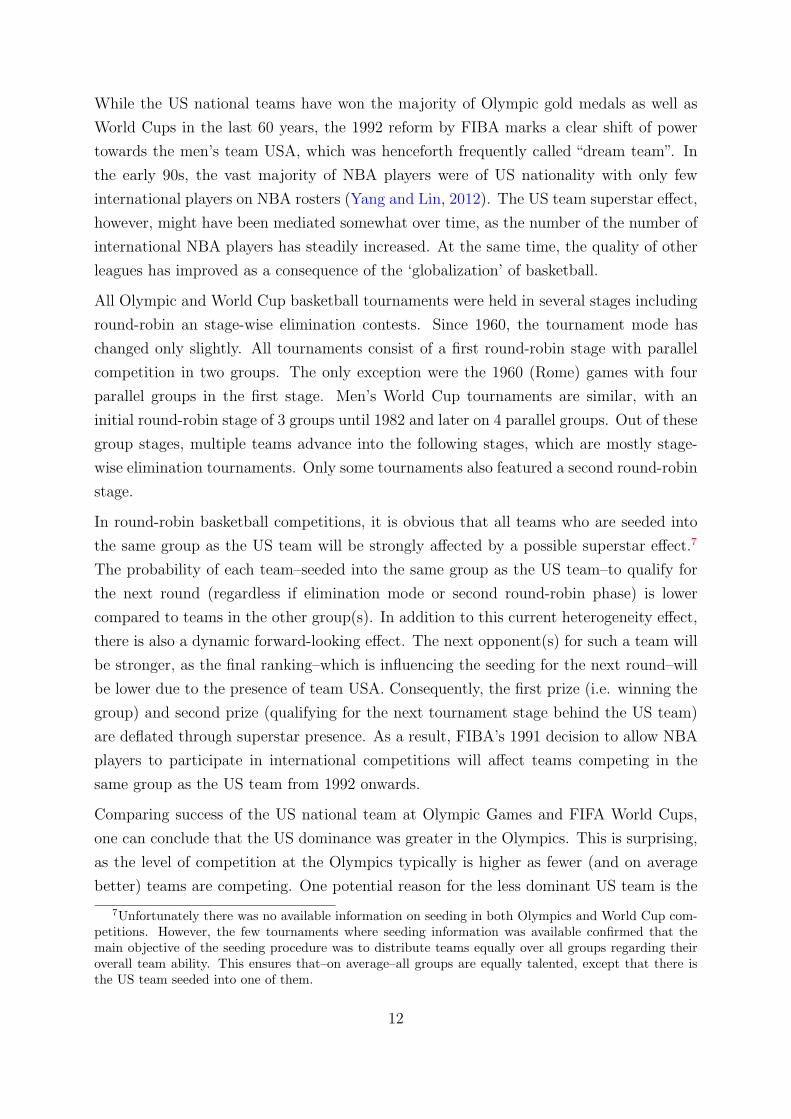
Table 5 plots the evolution of the average number of personal fouls per player-minute

over three time intervals (decades), before and after the reform in 1992. When comparing

games in the same group as team USA with all other games (top left panel), we see an

accelerating downward trend after the 1992 reform, which was more pronounced compared

to all other games. Looking at Olympic games (top right panel) and World Cups (lower

left panel) separately, we see that this seems to be coming mostly from Olympic games.

In addition, it is obvious that the common trend assumption is not violated.

13

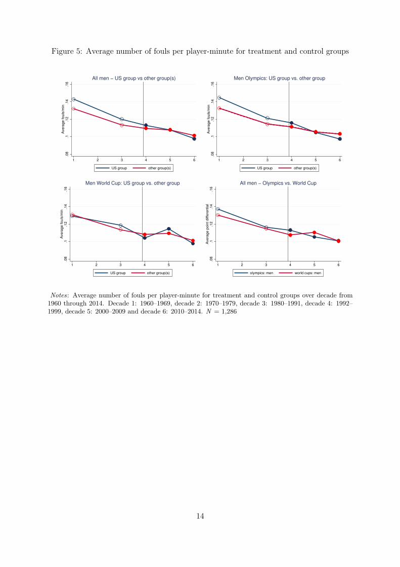
Figure 5: Average number of fouls per player-minute for treatment and control groups

.08

.1.1

2.1

4.1

6A

vera

ge fouls

/min

1 2 3 4 5 6

US group other group(s)

All men − US group vs other group(s)

.08

.1.1

2.1

4.1

6A

vera

ge fouls

/min

1 2 3 4 5 6

US group other group(s)

Men Olympics: US group vs. other group

.08

.1.1

2.1

4.1

6A

vera

ge fouls

/min

1 2 3 4 5 6

US group other group(s)

Men World Cup: US group vs. other group

.08

.1.1

2.1

4.1

6A

vera

ge p

oin

t diffe

rential

1 2 3 4 5 6

olympics: men world cups: men

All men − Olympics vs. World Cup

Notes: Average number of fouls per player-minute for treatment and control groups over decade from1960 through 2014. Decade 1: 1960–1969, decade 2: 1970–1979, decade 3: 1980–1991, decade 4: 1992–1999, decade 5: 2000–2009 and decade 6: 2010–2014. N = 1,286

14

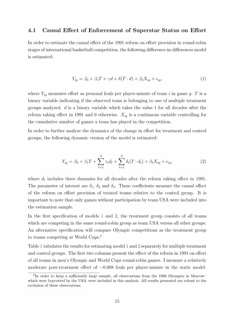
4.1 Causal Effect of Enforcement of Superstar Status on Effort

In order to estimate the causal effect of the 1991 reform on effort provision in round-robin

stages of international basketball competition, the following difference-in-differences model

is estimated:

Yig = β0 + β1T + γd+ δ(T · d) + β3Xig + ǫig, (1)

where Yig measures effort as personal fouls per player-minute of team i in game g. T is a

binary variable indicating if the observed team is belonging to one of multiple treatment

groups analyzed. d is a binary variable which takes the value 1 for all decades after the

reform taking effect in 1991 and 0 otherwise. Xig is a continuous variable controlling for

the cumulative number of games a team has played in the competition.

In order to further analyze the dynamics of the change in effort for treatment and control

groups, the following dynamic version of the model is estimated:

Yig = β0 + β1T +3∑

t=1

γtdt +3∑

t=1

δt(T · dt) + β3Xig + ǫig, (2)

where dt includes three dummies for all decades after the reform taking effect in 1991.

The parameter of interest are δ1, δ2 and δ3. These coefficients measure the causal effect

of the reform on effort provision of treated teams relative to the control group. It is

important to note that only games without participation by team USA were included into

the estimation sample.

In the first specification of models 1 and 2, the treatment group consists of all teams

which are competing in the same round-robin group as team USA versus all other groups.

An alternative specification will compare Olympic competitions as the treatment group

to teams competing at World Cups.8

Table 1 tabulates the results for estimating model 1 and 2 separately for multiple treatment

and control groups. The first two columns present the effect of the reform in 1991 on effort

of all teams in men’s Olympic and World Cups round-robin games. I measure a relatively

moderate post-treatment effect of −0.008 fouls per player-minute in the static model.

8In order to keep a sufficiently large sample, all observations from the 1980 Olympics in Moscow–which were boycotted by the USA–were included in this analysis. All results presented are robust to theexclusion of these observations.

15

This amounts to an increase of 10% on the sample mean or roughly 1.6 fouls less for a

standard game duration of 40 minutes.

The dynamic specification measures no significant decline in effort provision for teams

competing in the same group as team USA in the first decade after the reform (1992-

1999). However, in the period from 2000-2009, an effort decrease of −0.013 (2.6 fouls per

40 minutes) is estimated, while for the years 2010-2014 the estimated negative superstar

effect on effort is −0.017 (3.4 fouls per 40 minutes). From these dynamic diff-in-diff results

one can conclude that the increase in superstar status needed one decade to manifest itself

and was not weakened by the increased number of international players competing in the

NBA.

In a further step, Olympic and World Cup tournaments are analyzed separately. The

estimated coefficients indicate that the overall negative effect of superstar presence is

predominantly coming from Olympic tournaments. I estimate significant and sizeable

effects of the 1991 reform on effort of teams competing in the US round-round group.

This is not the case for the World Cup sample, where all estimated coefficients (static and

dynamic) are insignificant and close to 0. This result is not surprising, as the dominance

of the men’s team USA was much stronger in the Olympics (consult section 3). Columns

(7) and (8) confirm this notion, as we estimate the causal effect of the 1991 reform on the

treatment group Olympics Games compared to the “placebo” control group of games at

World Cups. Indeed I do estimate a negative effect of the reform on effort for the Olympic

Games. Thus, the reform was affecting mostly Olympic tournaments. Figure 6 plots the

estimated coefficients of the dynamic diff-in-diff model over time.

16

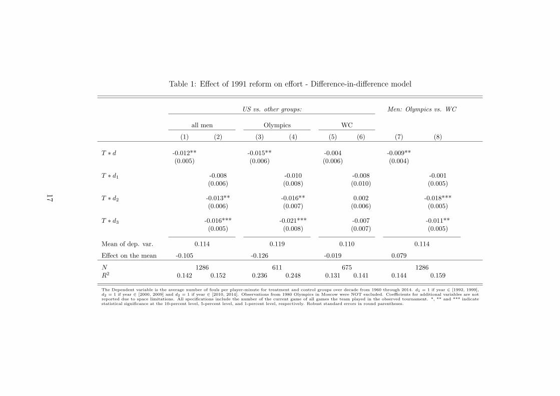
Table 1: Effect of 1991 reform on effort - Difference-in-difference model

US vs. other groups: Men: Olympics vs. WC

all men Olympics WC

(1) (2) (3) (4) (5) (6) (7) (8)

T ∗ d -0.012** -0.015** -0.004 -0.009**(0.005) (0.006) (0.006) (0.004)

T ∗ d1 -0.008 -0.010 -0.008 -0.001(0.006) (0.008) (0.010) (0.005)

T ∗ d2 -0.013** -0.016** 0.002 -0.018***(0.006) (0.007) (0.006) (0.005)

T ∗ d3 -0.016*** -0.021*** -0.007 -0.011**(0.005) (0.008) (0.007) (0.005)

Mean of dep. var. 0.114 0.119 0.110 0.114

Effect on the mean -0.105 -0.126 -0.019 0.079

N 1286 611 675 1286R2 0.142 0.152 0.236 0.248 0.131 0.141 0.144 0.159

The Dependent variable is the average number of fouls per player-minute for treatment and control groups over decade from 1960 through 2014. d1 = 1 if year ∈ [1992, 1999],d2 = 1 if year ∈ [2000, 2009] and d2 = 1 if year ∈ [2010, 2014]. Observations from 1980 Olympics in Moscow were NOT excluded. Coefficients for additional variables are notreported due to space limitations. All specifications include the number of the current game of all games the team played in the observed tournament. *, ** and *** indicatestatistical significance at the 10-percent level, 5-percent level, and 1-percent level, respectively. Robust standard errors in round parentheses.

17

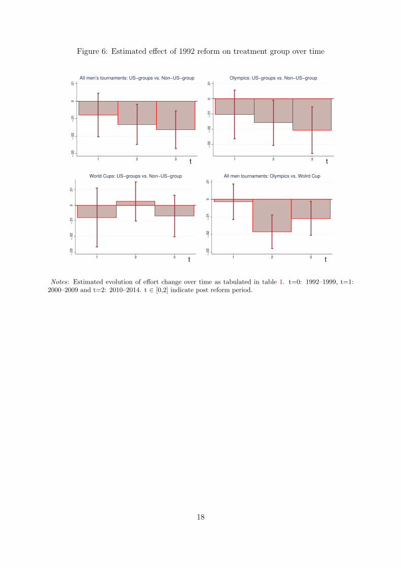
Figure 6: Estimated effect of 1992 reform on treatment group over time

−.0

3−

.02

−.0

10

.01

1 2 3 t

All men’s tournaments: US−groups vs. Non−US−group

−.0

3−

.02

−.0

10

.01

1 2 3 t

Olympics: US−groups vs. Non−US−group

−.0

3−

.02

−.0

10

.01

1 2 3 t

World Cups: US−groups vs. Non−US−group

−.0

3−

.02

−.0

10

.01

1 2 3 t

All men tournaments: Olympics vs. Wolrd Cup

Notes: Estimated evolution of effort change over time as tabulated in table 1. t=0: 1992–1999, t=1:2000–2009 and t=2: 2010–2014. t ∈ [0,2] indicate post reform period.

18

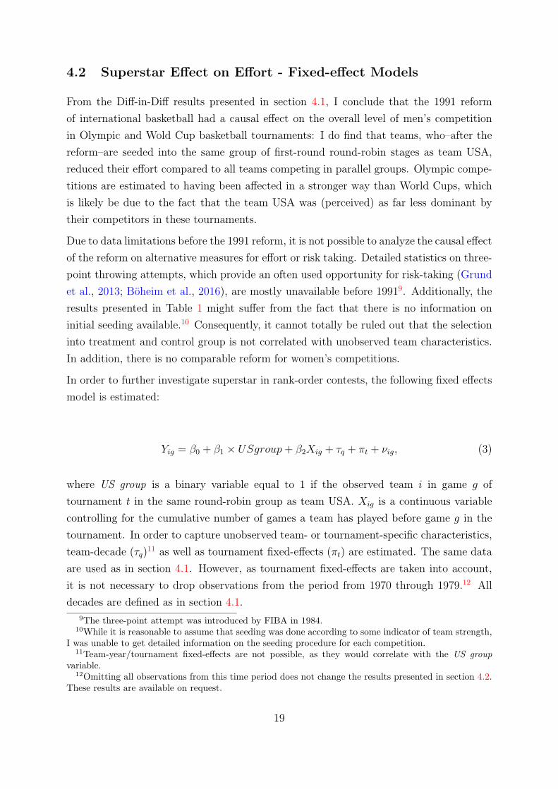
4.2 Superstar Effect on Effort - Fixed-effect Models

From the Diff-in-Diff results presented in section 4.1, I conclude that the 1991 reform

of international basketball had a causal effect on the overall level of men’s competition

in Olympic and Wold Cup basketball tournaments: I do find that teams, who–after the

reform–are seeded into the same group of first-round round-robin stages as team USA,

reduced their effort compared to all teams competing in parallel groups. Olympic compe-

titions are estimated to having been affected in a stronger way than World Cups, which

is likely be due to the fact that the team USA was (perceived) as far less dominant by

their competitors in these tournaments.

Due to data limitations before the 1991 reform, it is not possible to analyze the causal effect

of the reform on alternative measures for effort or risk taking. Detailed statistics on three-

point throwing attempts, which provide an often used opportunity for risk-taking (Grund

et al., 2013; Boheim et al., 2016), are mostly unavailable before 19919. Additionally, the

results presented in Table 1 might suffer from the fact that there is no information on

initial seeding available.10 Consequently, it cannot totally be ruled out that the selection

into treatment and control group is not correlated with unobserved team characteristics.

In addition, there is no comparable reform for women’s competitions.

In order to further investigate superstar in rank-order contests, the following fixed effects

model is estimated:

Yig = β0 + β1 × USgroup+ β2Xig + τq + πt + νig, (3)

where US group is a binary variable equal to 1 if the observed team i in game g of

tournament t in the same round-robin group as team USA. Xig is a continuous variable

controlling for the cumulative number of games a team has played before game g in the

tournament. In order to capture unobserved team- or tournament-specific characteristics,

team-decade (τq)11 as well as tournament fixed-effects (πt) are estimated. The same data

are used as in section 4.1. However, as tournament fixed-effects are taken into account,

it is not necessary to drop observations from the period from 1970 through 1979.12 All

decades are defined as in section 4.1.

9The three-point attempt was introduced by FIBA in 1984.10While it is reasonable to assume that seeding was done according to some indicator of team strength,

I was unable to get detailed information on the seeding procedure for each competition.11Team-year/tournament fixed-effects are not possible, as they would correlate with the US group

variable.12Omitting all observations from this time period does not change the results presented in section 4.2.

These results are available on request.

19

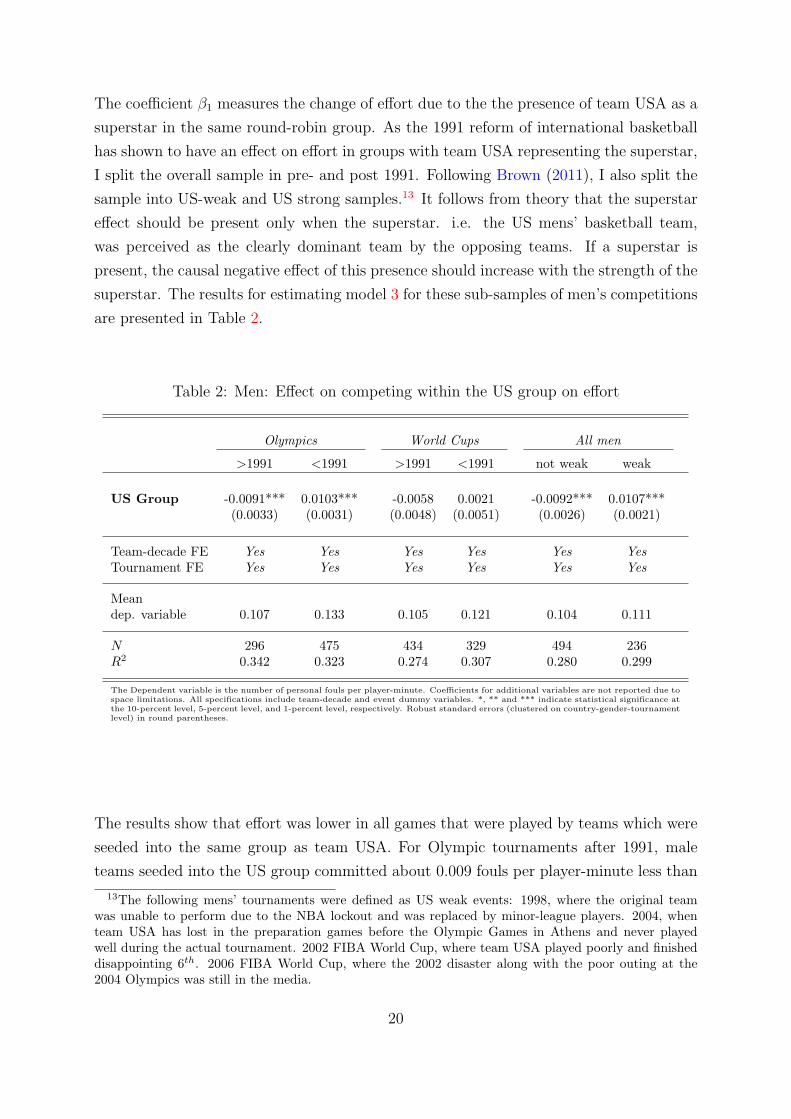
The coefficient β1 measures the change of effort due to the the presence of team USA as a

superstar in the same round-robin group. As the 1991 reform of international basketball

has shown to have an effect on effort in groups with team USA representing the superstar,

I split the overall sample in pre- and post 1991. Following Brown (2011), I also split the

sample into US-weak and US strong samples.13 It follows from theory that the superstar

effect should be present only when the superstar. i.e. the US mens’ basketball team,

was perceived as the clearly dominant team by the opposing teams. If a superstar is

present, the causal negative effect of this presence should increase with the strength of the

superstar. The results for estimating model 3 for these sub-samples of men’s competitions

are presented in Table 2.

Table 2: Men: Effect on competing within the US group on effort

Olympics World Cups All men

>1991 <1991 >1991 <1991 not weak weak

US Group -0.0091*** 0.0103*** -0.0058 0.0021 -0.0092*** 0.0107***(0.0033) (0.0031) (0.0048) (0.0051) (0.0026) (0.0021)

Team-decade FE Yes Yes Yes Yes Yes Yes

Tournament FE Yes Yes Yes Yes Yes Yes

Meandep. variable 0.107 0.133 0.105 0.121 0.104 0.111

N 296 475 434 329 494 236R2 0.342 0.323 0.274 0.307 0.280 0.299

The Dependent variable is the number of personal fouls per player-minute. Coefficients for additional variables are not reported due tospace limitations. All specifications include team-decade and event dummy variables. *, ** and *** indicate statistical significance atthe 10-percent level, 5-percent level, and 1-percent level, respectively. Robust standard errors (clustered on country-gender-tournamentlevel) in round parentheses.

The results show that effort was lower in all games that were played by teams which were

seeded into the same group as team USA. For Olympic tournaments after 1991, male

teams seeded into the US group committed about 0.009 fouls per player-minute less than

13The following mens’ tournaments were defined as US weak events: 1998, where the original teamwas unable to perform due to the NBA lockout and was replaced by minor-league players. 2004, whenteam USA has lost in the preparation games before the Olympic Games in Athens and never playedwell during the actual tournament. 2002 FIBA World Cup, where team USA played poorly and finisheddisappointing 6th. 2006 FIBA World Cup, where the 2002 disaster along with the poor outing at the2004 Olympics was still in the media.

20

all teams seeded into parallel groups. For competitions between 1960 and 1991 (before

the reform), I find that effort for teams competing in the US group was actually higher, as

teams commit about 0.010 fouls per player-minute more when seeded together with team

USA. This indicates that there was a pro-competitive peer-effect rather than a detrimental

superstar effect before the 1991 reform dramatically enforced the US superstar status. For

FIBA World Cups, I find a similar pro-competitive effect before 1991, while there is no

superstar effect to be found after the reform. This confirms the findings presented in

Table 1.

From the fixed-effects results one can cautiously conclude that the degree of dominance of

team USA–although yielding multiple Olympic and World Cup titles–was not big enough

before 1991 to cause an effort reducing superstar effect. Indeed, I do find a positive effort

enhancing effect of being seeded into the same group as the US team. When splitting

all competitions into tournaments where team USA was dominant and events where it

was performing below average, I find a negative but insignificant effect of the US team in

being seeded into the same group. For all years with a weak US team there is a strong

and significant pro-competitive effect.

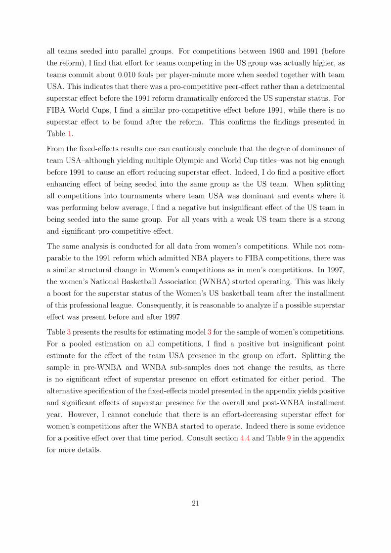
The same analysis is conducted for all data from women’s competitions. While not com-

parable to the 1991 reform which admitted NBA players to FIBA competitions, there was

a similar structural change in Women’s competitions as in men’s competitions. In 1997,

the women’s National Basketball Association (WNBA) started operating. This was likely

a boost for the superstar status of the Women’s US basketball team after the installment

of this professional league. Consequently, it is reasonable to analyze if a possible superstar

effect was present before and after 1997.

Table 3 presents the results for estimating model 3 for the sample of women’s competitions.

For a pooled estimation on all competitions, I find a positive but insignificant point

estimate for the effect of the team USA presence in the group on effort. Splitting the

sample in pre-WNBA and WNBA sub-samples does not change the results, as there

is no significant effect of superstar presence on effort estimated for either period. The

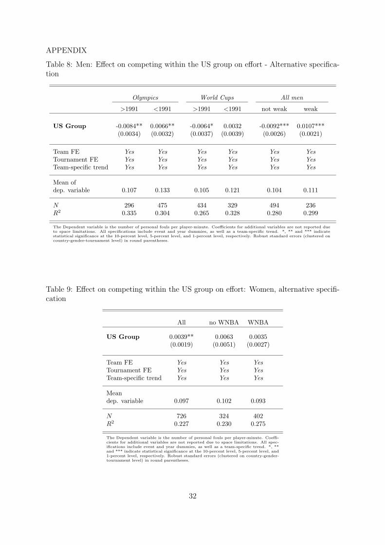
alternative specification of the fixed-effects model presented in the appendix yields positive

and significant effects of superstar presence for the overall and post-WNBA installment

year. However, I cannot conclude that there is an effort-decreasing superstar effect for

women’s competitions after the WNBA started to operate. Indeed there is some evidence

for a positive effect over that time period. Consult section 4.4 and Table 9 in the appendix

for more details.

21

Table 3: Women: Effect on competing within the US group on effort

All no WNBA WNBA

US Group 0.0013 0.0027 -0.0005(0.0026) (0.0046) (0.0037)

Team-decade FE Yes Yes Yes

Tournament FE Yes Yes Yes

Meandep. variable 0.097 0.102 0.093

N 726 324 402R2 0.270 0.242 0.291

The Dependent variable is the number of personal fouls per player-minute. Co-efficients for additional variables are not reported due to space limitations. Allspecifications include team-decade and event dummy variables. *, ** and *** in-dicate statistical significance at the 10-percent level, 5-percent level, and 1-percentlevel, respectively. Robust standard errors (clustered on country-gender-tournamentlevel) in round parentheses.

4.3 Risk Taking Behavior

There is little empirical evidence from the field on the effect of competitors’ heterogeneity

or superstar presence in competitions on agents’ or teams risk taking behavior. In a

theoretical article, Cabral (2003) analyzes how two agents decide between a safe and a

risky technology depending on whether they are trailing or leading in a R&D contest.

Heterogeneity in abilities can also be interpreted as a (score) deficit in a competition.

The weaker contestant is initially behind, as her/his probability to win the competition

is lower. Consequently, a deficit in abilities should increase a contestant’s willingness to

incur risks.

Brown (2011) identifies risk taking in professional golf contest, but her analysis fails to

identify any effect of superstar presence on risk taking of all other professional golf players

in top-tier tournaments. Another analysis is provided by Hill (2014), who uses false starts

as indicators for risk taking. The results indicate no (causal) effect of superstar presence

on risk taking in top-level 100 meter sprint competitions.

Following a definition of risk taking in basketball contests introduced by Grund et al.

(2013), I will examine if superstar presence has any effect on risk taking by professional

basketball teams in round-robin tournaments. Risk taking will be measured by the ratio

22

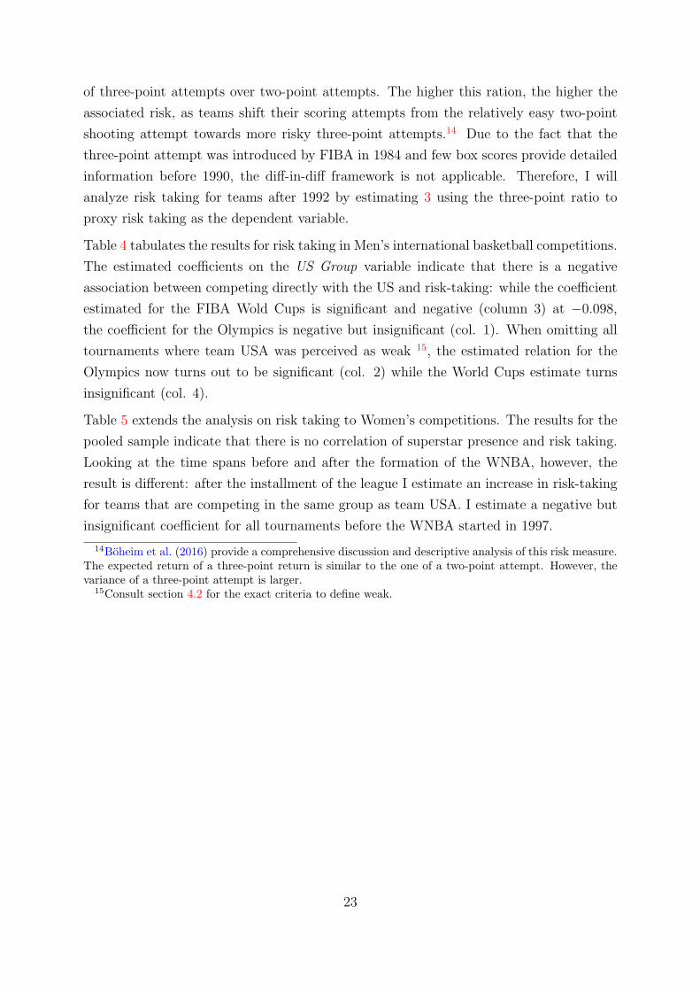
of three-point attempts over two-point attempts. The higher this ration, the higher the

associated risk, as teams shift their scoring attempts from the relatively easy two-point

shooting attempt towards more risky three-point attempts.14 Due to the fact that the

three-point attempt was introduced by FIBA in 1984 and few box scores provide detailed

information before 1990, the diff-in-diff framework is not applicable. Therefore, I will

analyze risk taking for teams after 1992 by estimating 3 using the three-point ratio to

proxy risk taking as the dependent variable.

Table 4 tabulates the results for risk taking in Men’s international basketball competitions.

The estimated coefficients on the US Group variable indicate that there is a negative

association between competing directly with the US and risk-taking: while the coefficient

estimated for the FIBA Wold Cups is significant and negative (column 3) at −0.098,

the coefficient for the Olympics is negative but insignificant (col. 1). When omitting all

tournaments where team USA was perceived as weak 15, the estimated relation for the

Olympics now turns out to be significant (col. 2) while the World Cups estimate turns

insignificant (col. 4).

Table 5 extends the analysis on risk taking to Women’s competitions. The results for the

pooled sample indicate that there is no correlation of superstar presence and risk taking.

Looking at the time spans before and after the formation of the WNBA, however, the

result is different: after the installment of the league I estimate an increase in risk-taking

for teams that are competing in the same group as team USA. I estimate a negative but

insignificant coefficient for all tournaments before the WNBA started in 1997.

14Boheim et al. (2016) provide a comprehensive discussion and descriptive analysis of this risk measure.The expected return of a three-point return is similar to the one of a two-point attempt. However, thevariance of a three-point attempt is larger.

15Consult section 4.2 for the exact criteria to define weak.

23

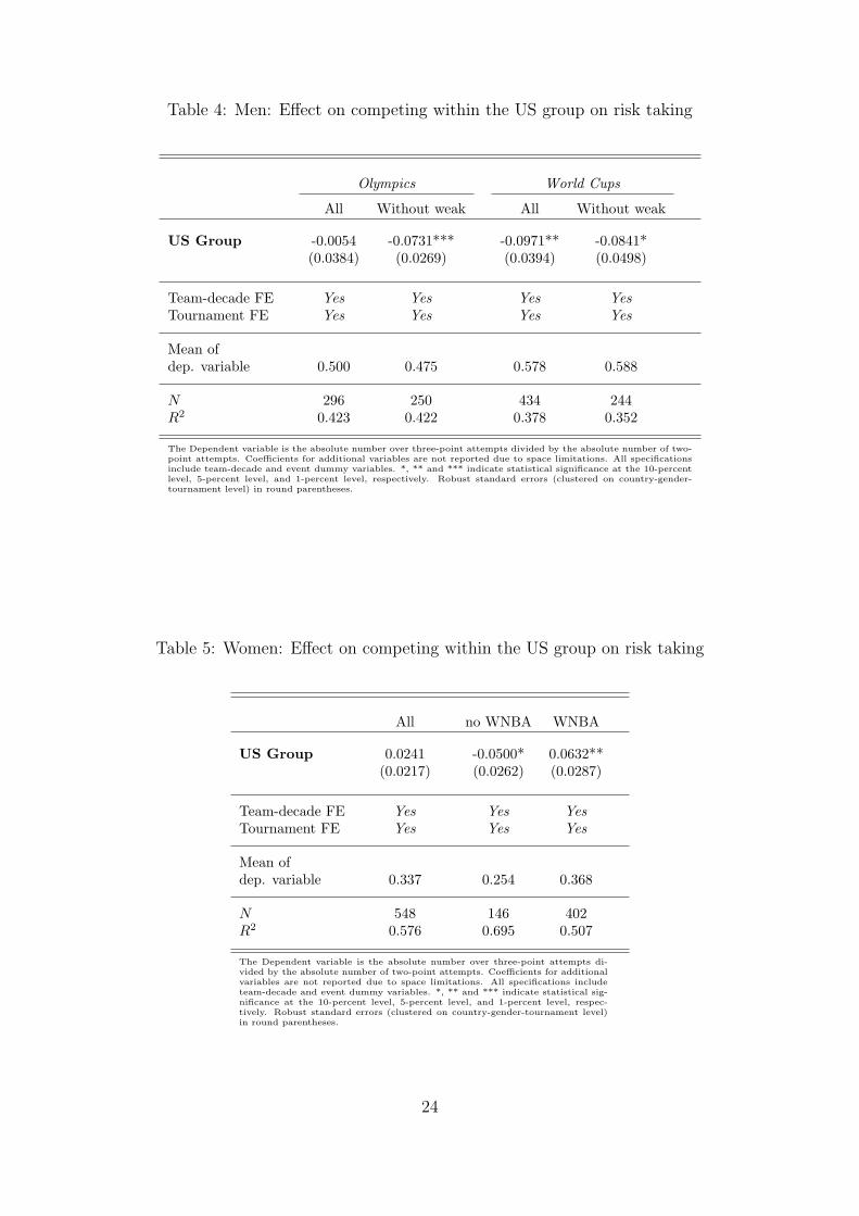
Table 4: Men: Effect on competing within the US group on risk taking

Olympics World Cups

All Without weak All Without weak

US Group -0.0054 -0.0731*** -0.0971** -0.0841*(0.0384) (0.0269) (0.0394) (0.0498)

Team-decade FE Yes Yes Yes Yes

Tournament FE Yes Yes Yes Yes

Mean ofdep. variable 0.500 0.475 0.578 0.588

N 296 250 434 244R2 0.423 0.422 0.378 0.352

The Dependent variable is the absolute number over three-point attempts divided by the absolute number of two-point attempts. Coefficients for additional variables are not reported due to space limitations. All specificationsinclude team-decade and event dummy variables. *, ** and *** indicate statistical significance at the 10-percentlevel, 5-percent level, and 1-percent level, respectively. Robust standard errors (clustered on country-gender-tournament level) in round parentheses.

Table 5: Women: Effect on competing within the US group on risk taking

All no WNBA WNBA

US Group 0.0241 -0.0500* 0.0632**(0.0217) (0.0262) (0.0287)

Team-decade FE Yes Yes Yes

Tournament FE Yes Yes Yes

Mean ofdep. variable 0.337 0.254 0.368

N 548 146 402R2 0.576 0.695 0.507

The Dependent variable is the absolute number over three-point attempts di-vided by the absolute number of two-point attempts. Coefficients for additionalvariables are not reported due to space limitations. All specifications includeteam-decade and event dummy variables. *, ** and *** indicate statistical sig-nificance at the 10-percent level, 5-percent level, and 1-percent level, respec-tively. Robust standard errors (clustered on country-gender-tournament level)in round parentheses.

24

4.4 Robustness

In sections 4.1 and 4.2, I use personal fouls as a proxy for effort. Alternatively, fouls

could be interpreted as sabotage. However, effort and sabotage–while being two distinct

phenomena–are obviously related: a foul which aims at stopping the opponent from scor-

ing as the only possible way also represents effort.

Linking the number of fouls to an increase in the probability to win a game is difficult and

not feasible with the underlying data.16 In order to add robustness to the analysis, the

number of points scored is used as alternative proxy for effort. In contrast to personal fouls,

however, the number of points scored per player-minute is measuring intermediate output

rather than a true effort input in the production function of teams. In addition, points

scored are measuring performance, which is not only affected by effort, but a multitude of

factors, including pure luck. Consequently, this additional approach represents a second

best strategy, as is is not measuring a strategic decision of teams but an (intermediate)

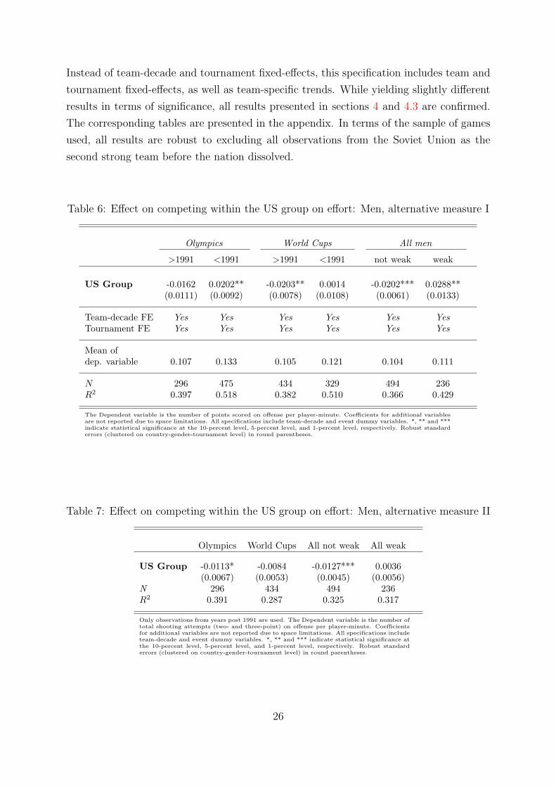
outcome. Table 6 tabulates the results from estimating model 3 with the number of points

scored per player-minute as the dependent variable.

The results confirm the earlier findings for the effect of superstar presence on effort: male

teams tend to exert less offensive effort (i.e. they score less) when they are in the same

group as team USA after the Olympics and Wold Cups allowed professional athletes to

participate. The coefficient for the Olympics is borderline insignificant but negative. In

year before the FIBA reform, we see a positive effect of superstar presence on (offensive)

effort. As before, I split the overall post 1991-reform sample into years where the US team

was anticipated to be weak or strong. When the US team was weak (strong), there is a

negative (positive) effect of superstar presence on effort.

Table 7 tabulates the results for using the absolute number of shooting attempts per

player-minute as a third effort proxy.17 In the presence of a strong superstar I estimate

a strong negative effect on this specific effort measure. The estimated effect for Olympic

Games and World Cups are also negative, albeit not highly significant. In the years when

the team USS was perceived weak, there is a small but insignificant positive effect of

superstar presence on the number of shooting attempts per player-minute. Consequently,

this results confirms the negative effect of superstar presence on (offensive) effort.

The empirical approach of section 4.2 controls for unobserved team heterogeneity by

estimating team-decade fixed effects in analogy to the timing effects presented in Table 1.

In order to test the robustness of these results, an alternative specification is estimated.

16Consult Lackner et al. (2015) for a detailed discussion of this issue.17As for the risk taking measure, the analysis of throwing attempts is restricted to the years after 1991.

Official FIBA box score statistics before do not report throwing attempts.

25

Instead of team-decade and tournament fixed-effects, this specification includes team and

tournament fixed-effects, as well as team-specific trends. While yielding slightly different

results in terms of significance, all results presented in sections 4 and 4.3 are confirmed.

The corresponding tables are presented in the appendix. In terms of the sample of games

used, all results are robust to excluding all observations from the Soviet Union as the

second strong team before the nation dissolved.

Table 6: Effect on competing within the US group on effort: Men, alternative measure I

Olympics World Cups All men

>1991 <1991 >1991 <1991 not weak weak

US Group -0.0162 0.0202** -0.0203** 0.0014 -0.0202*** 0.0288**(0.0111) (0.0092) (0.0078) (0.0108) (0.0061) (0.0133)

Team-decade FE Yes Yes Yes Yes Yes Yes

Tournament FE Yes Yes Yes Yes Yes Yes

Mean ofdep. variable 0.107 0.133 0.105 0.121 0.104 0.111

N 296 475 434 329 494 236R2 0.397 0.518 0.382 0.510 0.366 0.429

The Dependent variable is the number of points scored on offense per player-minute. Coefficients for additional variablesare not reported due to space limitations. All specifications include team-decade and event dummy variables. *, ** and ***indicate statistical significance at the 10-percent level, 5-percent level, and 1-percent level, respectively. Robust standarderrors (clustered on country-gender-tournament level) in round parentheses.

Table 7: Effect on competing within the US group on effort: Men, alternative measure II

Olympics World Cups All not weak All weak

US Group -0.0113* -0.0084 -0.0127*** 0.0036(0.0067) (0.0053) (0.0045) (0.0056)

N 296 434 494 236R2 0.391 0.287 0.325 0.317

Only observations from years post 1991 are used. The Dependent variable is the number oftotal shooting attempts (two- and three-point) on offense per player-minute. Coefficientsfor additional variables are not reported due to space limitations. All specifications includeteam-decade and event dummy variables. *, ** and *** indicate statistical significance atthe 10-percent level, 5-percent level, and 1-percent level, respectively. Robust standarderrors (clustered on country-gender-tournament level) in round parentheses.

26

5 Conclusion

I use data from top-level international basketball contests to analyze superstar effects

in the context of rank-order tournaments. A superstar in my context is a team which

dominates competitions over a substantial period of time. The data identifies team USA

in men’s and women’s national basketball competitions as superstars. A Descriptive

analysis confirms that the US men’s national basketball team was indeed the dominant

team in international competitions. However, the degree of dominance fluctuated as a

result of an exogenous institutional reform. In addition, I use the US women’s basketball

team as a second superstar in order to test for potential gender differences in superstar

effects.

In the empirical analysis I find that there is a causal effect of superstar presence for men’s

Olympic tournaments. Results from a diff-in-diff model suggest that this causal effect is

due to the enforcement of the dominance or status of the sole superstar through a reform

in 1992. This confirms theoretical results that demonstrate an increase superstar effect if

superstar status gets stronger (Brown, 2011). There is also evidence to conclude that not

only performance dominance but also status (financial) dominance plays a significant role,

as the 1992 reform did not only enforce performance related dominance of team USA. It

did also push the team’s status as a superstar with a vastly superior status in terms of

income and popularity.

I find significant and sizeable negative superstar effects on effort if the superstar was indeed

dominant. Before the reform of 1992 and in competitions where team USA was perceived

as weak, competition within the same group of the superstar yields higher effort. This

finding of a positive peer effect further extends Brown (2011) and confirms the findings

of Hill (2012).

In a second step, I analyze the effect of superstar presence on risk-taking behavior of male

and female teams. For male teams, I do find robust evidence for a reduction of risk-taking

if team USA as the superstar is present. For women, however, I get mixed results. Before

the initiation of the leading professional women’s basketball league (WNBA) in the US,

there is a similar negative relationship between risk-taking and superstar presence. After

the WNBA was initiated in 1997, this relationship is positive.

The results presented in this article have strong implications in a multitude of different

contexts. Superstar effects are highly relevant for the design of promotion- and other

types of tournaments. A firm typically wants to maximize total effort of all contestants

by designing a tournament for ultimately selecting the best candidate. If a sufficiently

strong superstar is present, a rank-order tournament design is not an optimal solution:

27

As all participants will consider their chances to rank higher than the superstar to be very

small, they will reduce effort. Consequently, superstar presence will reduce overall effort

and work against the target of overall effort maximization. In addition R&D contests or

patent races will also be affected by the presence of a superstar firm. Such a dominant

firm will reduce effort of all competing firms, which will have a negative effect on overall

effort. Considering the overall reduction in investment into research and development

(ie.e effort), this will likely lead to a loss in total welfare.

My finding of a positive peer effect in the presence of a weak superstar (or multiple

superstars) are of high relevance. However, more research is needed in order to understand

when a superstar peer effect actually does turn into a detrimental effort reducing superstar

effect.

28

References

Baik, Kyung Hwan, “Effort levels in contests with two asymmetric players,” Southern

Economic Journal, 1994, 61 (2), 367–379.

Berger, Johannes and Petra Nieken, “Heterogeneous Contestants and the Intensity

of Tournaments An Empirical Investigation,” Journal of Sports Economics, 2014.

Boheim, Rene, Christoph Freudenthaler, and Mario Lackner, “Gender Differ-

ences in Risk-Taking: Evidence from Professional Basketball,” IZA Discussion Paper,

2016. [accessed on 1 August 2016].

Boudreau, Kevin J, Nicola Lacetera, and Karim R Lakhani, “Incentives and

Problem Uncertainty in Innovation Contests: An Empirical Analysis,” Management

Science, 2011, 57 (5), 843–863.

Brandes, Leif, Egon Franck, and Stephan Nuesch, “Local heroes and superstars: An

empirical analysis of star attraction in German soccer,” Journal of Sports Economics,

2008, 9 (3).

Brown, Jennifer, “Quitters Never Win: The (Adverse) Incentive Effects of Competing

With Superstars,” Journal of Political Economy, 2011, 119 (5), 982–1013.

and Dylan B. Minor, “Selecting the Best? Spillover and Shadows in Elimination

Tournaments,”Management Science, 2014, 60 (12), 3087–3102.

Cabral, Luis, “R&D competition when firms choose variance,” Journal of Economics &

Management Strategy, 2003, 12 (1), 139–150.

Chan, Tat Y, Jia Li, and Lamar Pierce, “Compensation and Peer Effects in Com-

peting Sales Teams,”Management Science, 2014.

Charness, Gary and Matthias Sutter, “Groups make better self-interested decisions,”

The Journal of Economic Perspectives, 2012, pp. 157–176.

Deutscher, Christian, Bernd Frick, Oliver Gurtler, and Joachim Prinz, “Sab-

otage in Tournaments with Heterogeneous Contestants: Empirical Evidence from the

Soccer Pitch,”The Scandinavian Journal of Economics, 2013, 115 (4), 1138–1157.

Emerson, Jamie and Brian C. Hill, “Gender Differences in Competition: Running

Performance in 1,500 Meter Tournaments,” Eastern Economic Journal, 2014, 40, 499–

517.

29

Fort, Rodney and James Quirk, “Cross-subsidization, incentives, and outcomes in

professional team sports leagues,” Journal of Economic Literature, 1995, 33 (3), 1265–

1299.

Grund, Christian, Jan Hocker, and Stefan Zimmermann, “Incidence and Conse-

quences of Risk Taking Behavior in Tournaments: Evidence from the NBA,”Economic

Inquiry, 2013, 51 (2), 1489–1501.

Hausman, Jerry A. and Gregory K. Leonard, “Superstars in the National Basketball

Association: Economic Value and Policy,” Journal of Labor Economics, 1997, 15 (4),

586–624.

Hill, Brian C., “The Heat Is On: Tournament Structure, Peer Effects, and Performance,”

Journal of Sports Economics, 2012, 15 (4), 515–337.

, “The Superstar Effect in 100-Meter Tournaments,” International Journal of Sport

Finance, 2014, 9 (2), 111–129.

Jane, Wen-Jhan, “Peer Effects and Individual Performance: Evidence From Swimming

Competitions,” Journal of Sports Economics, 2014.

Kocher, Martin G and Matthias Sutter, “The Decision Maker Matters: Individ-

ual Versus Group Behaviour in Experimental Beauty-Contest Games,” The Economic

Journal, 2005, 115 (500), 200–223.

Krueger, Alan B, “The economics of real superstars: The market for rock concerts in

the material world,” Journal of Labor Economics, 2005, 23 (1), 1–30.

Kuethe, Todd H and Mesbah Motamed, “Returns to stardom: evidence from US

major league soccer,” Journal of Sports Economics, 2010, 11 (5), 567–579.

Lackner, Mario, Rudi Stracke, Uwe Sunde, and Rudolf Winter-Ebmer, “Are

Competitors Forward Looking in Strategic Interactions? Evidence from the Field,” IZA

Discussion Papers 9564, Institute for the Study of Labor (IZA) 2015. [accessed on 1

May 2016].

Lazear, Edward P and Sherwin Rosen, “Rank-Order Tournaments as Optimum

Labor Contracts,”The Journal of Political Economy, 1981, 89 (5), 841–864.

Lucifora, Claudio and Rob Simmons, “Superstar effects in sport evidence from Italian

soccer,” Journal of Sports Economics, 2003, 4 (1), 35–55.

30

Malmendier, Ulrike and Geoffrey Tate, “Superstar CEOs,” The Quarterly Journal

of Economics, 2009, 124 (4), 1593–1638.

Nieken, Petra and Michael Stegh, “Incentive Effects in Asymmetric Tournaments

Empirical Evidence from the German Hockey League,”mimeo, 2010.

Rosen, Sherwin, “The economics of superstars,” American Economic Review, 1981, 71

(5), 845–858.

, “Prizes and Incentives in Elimination Tournaments,” American Economic Review,

1986, 76 (4), 701–715.

Stracke, Rudi and Uwe Sunde, “Dynamic Incentive Effects of Heterogeneity in Multi-

Stage Promotion Contests,”mimeo, 2014. [accessed on 1 June 2016].

, Wolfgang Hochtl, Rudolf Kerschbamer, and Uwe Sunde, “Incentives and selec-

tion in promotion contests: Is it possible to kill two birds with one stone?,”Managerial

and Decision Economics, 2015, 36 (5), 275–285.

Sunde, Uwe, “Heterogeneity and performance in tournaments: a test for incentive effects

using professional tennis data,”Applied Economics, 2009, 41 (25), 3199–3208.

Szymanski, Stefan, “The Economic Design of Sporting Contests,” Journal of Economic

Literature, 2003, 41 (4), 1137–1187.

Yang, Chih-Hai and Hsuan-Yu Lin, “Is there salary discrimination by nationality in

the NBA? Foreign talent or foreign market,” Journal of Sports Economics, 2012, 13 (1),

53–75.

31

APPENDIX

Table 8: Men: Effect on competing within the US group on effort - Alternative specifica-tion

Olympics World Cups All men

>1991 <1991 >1991 <1991 not weak weak

US Group -0.0084** 0.0066** -0.0064* 0.0032 -0.0092*** 0.0107***(0.0034) (0.0032) (0.0037) (0.0039) (0.0026) (0.0021)

Team FE Yes Yes Yes Yes Yes Yes

Tournament FE Yes Yes Yes Yes Yes Yes

Team-specific trend Yes Yes Yes Yes Yes Yes

Mean ofdep. variable 0.107 0.133 0.105 0.121 0.104 0.111

N 296 475 434 329 494 236R2 0.335 0.304 0.265 0.328 0.280 0.299

The Dependent variable is the number of personal fouls per player-minute. Coefficients for additional variables are not reported dueto space limitations. All specifications include event and year dummies, as well as a team-specific trend. *, ** and *** indicatestatistical significance at the 10-percent level, 5-percent level, and 1-percent level, respectively. Robust standard errors (clustered oncountry-gender-tournament level) in round parentheses.

Table 9: Effect on competing within the US group on effort: Women, alternative specifi-cation

All no WNBA WNBA

US Group 0.0039** 0.0063 0.0035(0.0019) (0.0051) (0.0027)

Team FE Yes Yes Yes

Tournament FE Yes Yes Yes

Team-specific trend Yes Yes Yes

Meandep. variable 0.097 0.102 0.093

N 726 324 402R2 0.227 0.230 0.275

The Dependent variable is the number of personal fouls per player-minute. Coeffi-cients for additional variables are not reported due to space limitations. All spec-ifications include event and year dummies, as well as a team-specific trend. *, **and *** indicate statistical significance at the 10-percent level, 5-percent level, and1-percent level, respectively. Robust standard errors (clustered on country-gender-tournament level) in round parentheses.

32

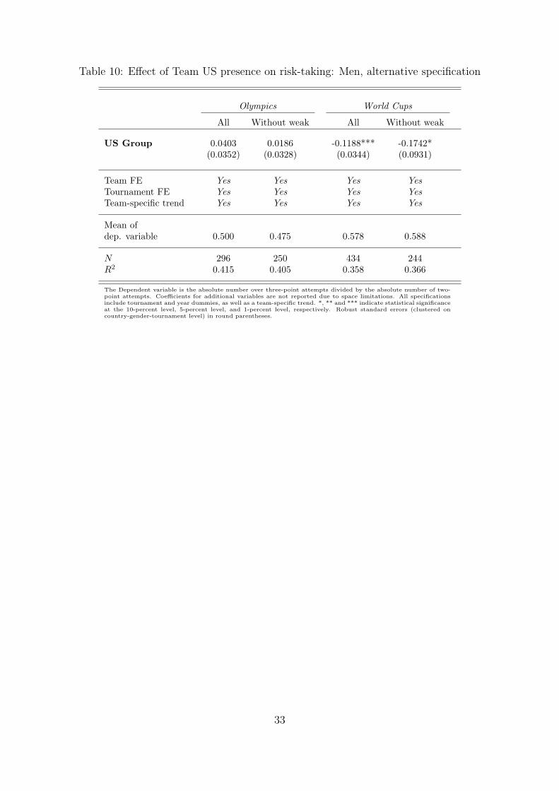
Table 10: Effect of Team US presence on risk-taking: Men, alternative specification

Olympics World Cups

All Without weak All Without weak

US Group 0.0403 0.0186 -0.1188*** -0.1742*(0.0352) (0.0328) (0.0344) (0.0931)

Team FE Yes Yes Yes Yes

Tournament FE Yes Yes Yes Yes

Team-specific trend Yes Yes Yes Yes

Mean ofdep. variable 0.500 0.475 0.578 0.588

N 296 250 434 244R2 0.415 0.405 0.358 0.366

The Dependent variable is the absolute number over three-point attempts divided by the absolute number of two-point attempts. Coefficients for additional variables are not reported due to space limitations. All specificationsinclude tournament and year dummies, as well as a team-specific trend. *, ** and *** indicate statistical significanceat the 10-percent level, 5-percent level, and 1-percent level, respectively. Robust standard errors (clustered oncountry-gender-tournament level) in round parentheses.

33

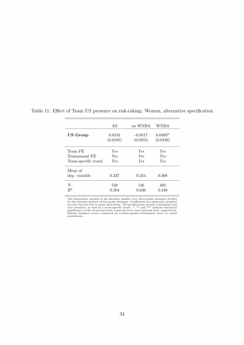
Table 11: Effect of Team US presence on risk-taking: Women, alternative specification

All no WNBA WNBA

US Group 0.0135 -0.0517 0.0493*(0.0185) (0.0355) (0.0246)

Team FE Yes Yes Yes

Tournament FE Yes Yes Yes

Team-specific trend Yes Yes Yes

Mean ofdep. variable 0.337 0.254 0.368

N 548 146 402R2 0.504 0.636 0.448

The Dependent variable is the absolute number over three-point attempts dividedby the absolute number of two-point attempts. Coefficients for additional variablesare not reported due to space limitations. All specifications include tournament andyear dummies, as well as a team-specific trend. *, ** and *** indicate statisticalsignificance at the 10-percent level, 5-percent level, and 1-percent level, respectively.Robust standard errors (clustered on country-gender-tournament level) in roundparentheses.

34