Team 520: Trane: Improve Air Quality

Team 520 i

2021

Jake S. Hamilton; Nicholas A. Holm; Andreu F. Santeiro; Joseph M. Thyer; Gavin A. Young

FAMU-FSU College of Engineering 2525 Pottsdamer St. Tallahassee, FL. 32310

Team 520: Trane: Improve Air Quality

4/13/2021

Team 520 ii

2021

Abstract

Due to the pressing times of COVID-19, an HVAC solution is needed to ensure air quality meets

the necessary requirements. This project is to identify and validate a sustainable HVAC solution

that improves air quality and adheres to government and environmental guidelines to combat

COVID-19. It will continue to be sustainable in future markets for residential and commercial

applications.

Keywords: HVAC, air quality, coronavirus, bipolar ionization, ionization

Team 520 iii

2021

Acknowledgement

We would like to thank our sponsor Cameron Griffith with Trane for taking the time to

meet with us to provide us with the necessary information about our project. We would also like

to thank Dr. McConomy and Dr. Ordonez for giving us mentorship throughout this project. We

also wish to thank Jim Stephens for giving us insight into FSU’s Utilities and Maintenance

operations.

Team 520 iv

2021

Table of Contents

Abstract .......................................................................................................................... ii

Disclaimer ....................................................................... Error! Bookmark not defined.

Acknowledgement ........................................................... Error! Bookmark not defined.

List of Tables................................................................................................................. vi

List of Figures .............................................................................................................. vii

Notation ...................................................................................................................... viii

Chapter One: EML 4551C ...............................................................................................9

1.1 Project Scope .........................................................................................................9

1.2 Customer Needs ................................................................................................... 12

1.3 Functional Decomposition ................................................................................... 16

1.4 Target Summary .................................................................................................. 19

1.5 Concept Generation ............................................................................................. 23

1.6 Concept Selection ................................................................................................ 29

Chapter Two: EML 4552C ............................................................................................ 34

2.1 Restated Project Definition & Scope .................................................................... 34

2.2 Results ................................................................................................................. 37

2.3 Discussion ........................................................................................................... 50

2.4 Conclusions ......................................................................................................... 51

Team 520 v

2021

2.5 Future Work......................................................................................................... 52

Appendix A: Code of Conduct ......................................... Error! Bookmark not defined.

Appendix B: Functional Decomposition ........................................................................ 54

Appendix C: Target Catalog .......................................................................................... 61

Appendix D: Concept Generation .................................................................................. 63

Appendix E: Concept Selection ..................................................................................... 75

Appendix F: MATLAB Code ........................................................................................ 76

Appendix G: Risk Assessment ..................................................................................... 120

References ................................................................................................................... 121

Team 520 vi

2021

List of Tables

Table 1) Cross-Reference Chart ……………………………………………………………………..8

Table 2) Critical Targets Summary ……………………………………………………………...…11

Table 3) House of Quality …………………………………………………………………...……….19

Table 4) Pairwise Comparison …………………………………...…………………………...…….20

Table 5) Pugh Matrix - 1…………………………………...…………………………………...…….21

Table 6) Pugh Matrix – 2 …………………………………...………………….………….…...…….22

Team 520 vii

2021

List of Figures

Figure 1) Negative Ion Concentration ………………………………………………...………….. 27

Figure 2) Positive Ion Concentration …………………………………………………….……….. 28

Figure 3) VOC Concentration …………………………………………………………..…..…….. 29

Figure 4-13) Mold Samples …………………………………………………………..…..……..39-49

Team 520 viii

2021

Notation

ACH – Air exchanges per hour

ASHRAE – American Society of Heating, Refrigeration and Air-Conditioning Engineers

CO2 – Carbon Dioxide

CDC – Centers for Disease Control and Prevention

EPA – Environmental Protection Agency

FAMU – Florida Agricultural and Mechanical University

FSU – Florida State University

HEPA – High-efficiency particulate air

HVAC – Heating, ventilation, and air conditioning

IAQ – Indoor Air Quality

IoT – Internet of Things

MERV – Minimum Efficiency Reporting Value

MRSA – Methicillin-Resistant Staphylococcus Aureus

OEM – Original Equipment Manufacturer

OSHA – Occupational Safety and Health Administration

PHI – Photo Hydro Ionization

PCO – Photocatalytic Oxidation

PPB – Parts Per Billion

PPM – Parts Per Million

UV – Ultra Violet

WHO – World Health Organization

VOC – Volatile Organic Compounds

Team 520 ix

2021

Chapter One: EML 4551C

1.1 Project Scope

Projection Description

The objective of this project is to develop and verify an HVAC solution that improves air

quality while adhering to current guidelines to combat COVID-19 and continue to sustainable in

future markets.

Key Goals

The primary goal of this project is to design an energy-efficient HVAC solution that

improves air quality and is sustainable for future markets when circumstances change. The

solution will adhere to government and environmental guidelines. A variety of technologies will

be investigated, and the most promising one will be pursued. The team will verify the usefulness

of the chosen solution, and a presentation will be given to Trane and FSU representatives to

present findings and offer the proposed solution.

Markets

Due to the increasing threat of the COVID-19 pandemic, air quality management is

critical in the effort to the slow of the virus. Any facility that requires adequate air quality,

humidity levels, and comfort is a potential market for this product. The primary markets are

Trane and FSU’s Utilities and Maintenance Department. Secondary markets include other

universities and schools, commercial buildings (hospitals, casinos, offices, bars, schools,

Team 520 10

2021

restaurants, stadiums, etc.), and residential buildings (homes, nursing homes, apartment

complexes, etc.).

Assumptions

The team has assumed that the solution will be compatible with existing systems, which

will eliminate the need for new infrastructure. The solution must adhere to all associated

government/environmental guidelines. School facilities may have limited availability or require

special guidelines to be followed due to the pandemic. The system will be tested in Florida

climate conditions.

The team has assumed that the solution will be compatible with existing systems, which

will eliminate the need for new infrastructure. The solution must adhere to all associated

government/environmental guidelines. School facilities may have limited availability or require

special guidelines to be followed due to the pandemic. The system will be tested in Florida

climate conditions.

Stakeholders

The stakeholders associated with this project include our senior design professor, Dr.

Shayne McConomy; our advisor, Dr. Juan Ordonez; our sponsor, Trane; our Trane liaison,

Cameron Griffith; FSU’s Utilities and Maintenance Executive Director, Jim Stephens; and the

City of Tallahassee Utilities. The users include indoor facilities that require proper ventilation to

ensure adequate air quality, humidity levels, and comfort within the premises. The beneficiaries

include those who are susceptible to COVID-19 (elderly, children, individuals with underlying

health problems).

Team 520 11

2021

Team 520 12

2021

1.2 Customer Needs

Questions and Answers:

Question 1: What is currently hindering Trane’s HVAC systems in terms of efficiency

and air quality?

Answer:

o OEM parts/equipment (York, Carrier, Daikin)

o Costly services

Interpretation: Outsourced equipment and maintenance costs make a large portion of

expenses. In house equipment will be used when possible, and maintenance cost will be a

consideration.

Question 2: What is expected of our team in terms of building a single component or a

complete system?

Answer: The team is expected to satisfy a need, regardless of whether it's through one

component or a complete system.

Interpretation: The project will take whatever form is required to achieve its goal.

Question 3: Has Trane made any changes regarding air quality during this COVID-19

pandemic? Can any improvements be made in terms of air quality & if so, how?

Answer: Research and development teams have been working on product testing

regarding the different variables associated with the HVAC system (component

specifications, component location within the system) to achieve the

Team 520 13

2021

recommended/optimal humidity levels and IAQ adhering to (ASHRAE, EPA, OSHA)

guidelines. New filter technologies including UV germicide filters and bipolar ionization

technology are being applied and researched due to these pressing times of the COVID-

19 pandemic. An improvement could be made in terms of air quality by increasing the air

exchange rate from 4-8 times per hour to something higher (8-10 times per hour?).

Interpretation: The system will improve air quality, and there are many potential

methods of doing so.

Question 4: What HVAC components are most prone to failure?

Answer: Depends on the system design and application.

Interpretation: Any component of Trane’s HVAC systems is available to be affected by

the project.

Question 5: What are the necessary attributes of a Trane HVAC system? (What

distinguishes a Trane from a Honeywell?)

Answer: Trane’s market consists of ⅓ residential applications and ⅔ commercial

applications. The company’s driven to provide the lowest life cycle cost, efficient

energy usage to reduce carbon emissions, and for sustainability in future markets.

Interpretation: The goals of the project will overlap with the goals of Trane.

Question 6: Will our team's design be focusing more on residential or commercial

applications?

Team 520 14

2021

Answer: Our team will be focused on air quality and efficiency in facilities like schools

and universities.

Interpretation: The project will be designed for use within facilities like schools and

universities.

Question 7: Are there any special programs used to design & analyze HVAC systems?

Will our team have access to these programs?

Answer: We are free to use any programs for this project, however, we might gain access

to Trane’s Trace 700 program.

Interpretation: The project is free to use whatever available software that will benefit

the design.

Question 8: Who are the stakeholders in this project?

Answer:

o Dr. McConomy - “Technical Buyer”

o Cameron Griffith - Senior Design Mentor (Trane Sponsor) “Executive Buyer”

o Jim Stevens - FSU HVAC Systems Coordinator

Interpretation: The different needs of different types of stakeholders will be met.

Question 9: What government/environmental regulations and guidelines are setting

Trane’s current product specifications?

Team 520 15

2021

Answer: No necessarily enforced regulations (yet), but there are guidelines given by

OSHA and the EPA.

Interpretation: Health and safety guidelines will be taken into consideration.

Question 10: What personal customer needs/wants does our team’s design need to

satisfy?

Answer: The implemented technology must continue to be useful/efficient after the

COVID-19 pandemic.

Interpretation: The design will continue to be useful throughout its lifecycle.

Explanation of Results:

The COVID-19 pandemic has made air quality issues more obvious. Our team sat down

with project sponsor Cameron Griffith to discuss ways we can help Trane create a

practical solution. There are many methods for improving air quality. However, all of

them negatively affect system efficiency. Our team is to design a system that maintains

excellent air quality without hurting the efficiency of existing HVAC systems. Because

air quality and system efficiency are general concerns, not specific to COVID-19, the

design will continue to be useful and cost-effective throughout its lifecycle.

Team 520 16

2021

1.3 Functional Decomposition

After meeting with our Project sponsor, we were told that the demand for clean building

air has never been greater. We learned that many existing HVAC systems are outdated. Many

HVAC systems do not exchange the air at a fast-enough rate to keep air from stagnating. Also,

we learned that existing advanced particulate filtering solutions are often cost prohibitive to

install and service. Based on our interpreted customer needs we divided the project into three

systems: Air Quality, Sustainability, and Controls. The first two systems directly satisfy our

customers' needs of improving air quality and system efficiency. Our third subsystem is to allow

controllability within the HVAC system and to monitor air quality data.

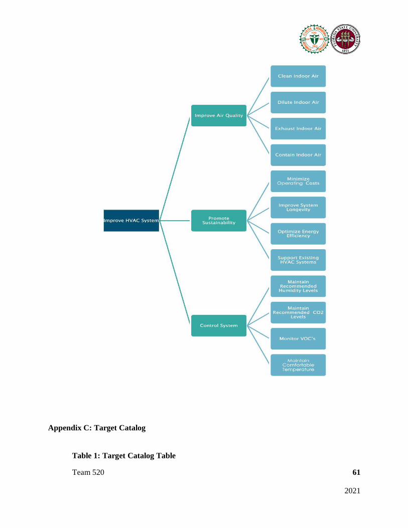
A hierarchical chart (Figure 2, Appendix B) based off of the functional decomposition

was created in order to visualize the breakdown of the project’s systems. The systems were then

expanded upon with desired functions. After creating the hierarchical chart, the systems were

then represented within a cross-reference table. This table allows functions to be compared

across the different systems for overlap of functionality.

The hierarchical chart illustrates the connection between systems and their functions. The

first system we chose was to improve air quality. The customer made it very clear that this is the

main priority of the system due to the COVID-19 pandemic. From the interpreted needs, we

determined our system needed to be able to clean, dilute, exhaust, and contain indoor air. Being

able to clean the air is important to rid the air of contaminants. Diluting the air is necessary to

exchange the old air with fresh air. Once the air is exchanged the old air needs to be safely

exhausted from the system. Finally, we want the system to contain clean air without leakage.

These four functions come directly from Trane; they are essential to good HVAC technology.

Team 520 17

2021

The next system identified by the team was to promote sustainability. A big problem with

improving air quality is that it typically decreases efficiency. We have been tasked with trying to

achieve both to the best of our ability. To promote sustainability within our system, we decided

our functions would be to: reduce operating costs, improve system longevity, optimize energy

efficiency, and support existing HVAC systems. When dealing with customer applications it is

always important to try and reduce installation and running costs. Budgets are often tight and

cannot accommodate large renovations. Improving the longevity of the system ensures that the

system remains useful in a post-COVID-19 environment. Optimizing energy efficiency vs

improved air quality is important. A grossly inefficient system will not result in a useful HVAC

system. Furthermore, our design needs to be capable of being retrofit onto existing systems. This

is important because it allows many potential use cases in different systems while also being less

than the cost of a replacement system. Our sponsor made it clear that practicing sustainable

engineering is important to Trane.

Our third system would be the controls aspect of the project. By monitoring certain

variables within the system, it allows the system to be more dynamic. It is important that the

system can respond to changing conditions. The functions identified were: maintain

recommended humidity levels and CO2 levels, a comfortable temperature, and monitor volatile

organic compounds (VOCs). It is important to maintain a humidity level that promotes both the

comfort of the inhabitants and the reduced growth of bacteria. Elevated CO2 levels can be

harmful and uncomfortable. A basic yet important function is that the system should maintain a

comfortable temperature. If an HVAC system cannot keep the building comfortable, then it has

failed its most basic duty. It is important to monitor and remove VOCs within the system as

Team 520 18

2021

inhabitants can inhale them and become sick. These four functions enable control of system to

the degree necessary to maintain air quality and promote sustainability.

The hierarchy chart was used to determine our basic functions. The cross-reference chart

is used to illustrate that some of these functions contribute to multiple sub-systems. Most of the

control functions are directly related to air quality. Maintaining humidity level is a function of

controls but is integral to air quality. The functional decomposition gives a better understanding

of the project by defining the relationships between each function. This understanding is useful

for concept generation and selection. The function resolution achieved in our functional

decomposition was defined well enough to convey the necessary design without constraining

certain aspects.

Table 1) Cross-Reference Chart

Team 520 19

2021

Table 1. Cross-Reference Chart

The functional decomposition illustrates what the project must accomplish

fundamentally. No matter what form it takes, the final project will be a controlled system that

improves air quality and promotes sustainability.

1.4 Target Summary

After defining the functions of the project in the function decomposition, methods for

defining and measuring those functions were examined.

There are four critical targets. If these four targets are met, the project will be a success.

Many of the other targets relate to these. A VOC concentration of 0.3 milligrams per cubic meter

is defined by the CDC as harmless air. There are conflicting data on this number. Erring on the

side of caution, 0.3 is on the lower end of recommended values (a lower concentration is better).

Team 520 20

2021

Air changes per hour (ACH) is how often the inside air is entirely exchanged for fresh air. The

CDC recommends different values based on the room in question. For example, chemical

facilities have higher recommended ACH than grocery stores. 10 ACH is on the high end for

applications for facilities like schools and office buildings. Energy usage and operating costs are

defined as a percentage of the value of the pre-existing system. When the project is implemented

into existing systems, energy usage will unavoidably increase, but a minimal increase is desired.

115% percent energy usage represents a 15% increase in energy use. This is an intermediate

value based on other air quality solutions. Operating costs directly related to energy use, but also

includes additional maintenance expenses on the additional system component. The desired

operating costs of the augmented system is 120% that of the existing system. These metrics are

defined so that they scale with the size of the existing system. The following table shows the

critical targets and metrics with their functions.

Table 2) Critical Targets Summary

Table 2. Critical Targets Summary Table

Other, noncritical functions are defined by the current guidelines for HVAC systems in

the United States. These standards are used because existing systems are already tested based on

them. The metrics are CO2 concentration, humidity control, and temperature control. The

functionality of the existing system must be unaffected by the implementation of the project.

Team 520 21

2021

There are two other functions that are also measured by ACH. Diluting the indoor air

directly means bringing in fresh air but exhausting and containing the air play an important role

as well. Each of them contributes uniquely to increasing ACH.

A table detailing each function with its respective metric and target can be found in

Appendix C.

Other needs are represented in these targets. It’s important that the project promotes the

ideals Trane uses to represent itself. Minimizing maintenance cost, and thus operating cost,

conveys a robust design with a long lifecycle. Minimizing energy usage connects to an

environmentally friendly mindset. Less energy usage means less carbon emissions. Notably,

none of the targets and metrics specifically mention COVID. To be a sound economic

investment, the system needs to be useful independent of COVID. Decreasing the VOC

concentration without a substantial increase in energy usage will always be an attractive feature.

If the critical metrics are measured, the project can be successfully validated. Testing for

energy usage is simple. Measuring the energy usage of the implemented design and comparing it

to the usage of the subject HVAC system gives all the necessary information. It is common

practice to estimate maintenance cost as a fraction of the initial cost a system. With this estimate

and energy usage, operating costs is easily calculated. ACH is just a function of the size of the

facility and the volumetric flow rate of the system, which can be measured in any number of

ways. Measuring the total VOC concentration is more difficult, as there are a variety of chemical

compounds that are identified as VOCs. To measure this accurately, a specialized device is

required. Due to limited resources, the device would have to be provided either by the college or

by Trane.

Team 520 22

2021

Many of these targets were determined from the functional decomposition and the

customer needs. Each one of these targets has an associated metric as to how to determine if the

targets are met. These metrics were determined largely through group research. For targets

related to air quality composition, the associated metric was found by consulting industry

standards set by ASHRAE and other regulatory agencies (EPA, OSHA, WHO). The installation

cost was found as the desired metric for fitting the HVAC system because the system should

require little to no modifications to be implemented. Optimizing energy efficiency was expressed

as a percentage as this function will scale with the size of the HVAC system. The energy usage

will increase for larger HVAC systems as they are used to cool larger areas. This same concept

explains why the operating costs were expressed as a percentage as well. This percentage was

larger than the energy efficiency as it must account for maintenance of the system as well as

energy usage.

Team 520 23

2021

1.5 Concept Generation

Methodology

There are many ways to approach improving air quality, which, fundamentally, the goal

of the project. There are any number of ways to fill a space with cleaner air. Air can be directly

cleaned. Indoor air can be diluted with fresh outdoor air. Many systems underperform to

conserve energy. Improvements in energy efficiency can lead to improved air quality without

increased energy expenditure. Energy can be found elsewhere and applied in a similar way.

As a result, there is no shortage of usable concepts. Many were provided as

recommendations from organizations like the CDC and ASHRAE. Some were offered as

interesting possibilities by Trane, and some are very minor changes to existing technology.

Most of the concepts came naturally, but the Crap Shoot method was also used. Everyone

is affected by air quality, and any indoor activity is as well. There are plenty of resources to draw

on to clean air. Because of this widespread, the Crap Shoot method seemed particularly useful.

Almost every possible combination resulted in a usable concept.

Furthermore, most air quality technologies are additive, so any number of them can be

used together. Solar panels can offset the energy usage of UV lights. UV lights can be used in

conjunction with high quality filters in particularly vulnerable areas. This lends itself to a

morphological chart, but because almost any solution can be combined with almost any other

solution, it wasn’t used.

The following concepts were chosen as the most promising. A summary is given of each.

They are further compared in Concept Selection. All generated concepts can be found in

Appendix D.

Team 520 24

2021

Medium Fidelity Concepts:

Concept 80. Implement antimicrobial coated duct lining to inhibit mold growth within

the ductwork and to make duct cleaning more feasible.

Assuming the current system duct lining installed, the inclusion of antimicrobial duct

lining would improve the system. The lining acts as an insulator which reduces energy

consumption and prevents unwanted water damage which can lead to costly damages. Adding

duct lining to an HVAC system also improves airflow by sealing any holes within the duct and

increases air quality if the lining is antimicrobial.

Concept 29: Implement Photo Hydro Ionization (PHI) as a purification technique to

increase air quality and reduce ozone levels.

An alternative purification technology developed by RGF Environmental Group is photo

hydro ionization (PHI). This technology utilizes UV lights and a catalyst to create hydro-

peroxide ions to deactivate harmful aerosols. During preliminary testing by Kansas State

University, PHI was proven effective against viruses and bacteria such as MRSA and Swine Flu.

Concept 91: Implement Photocatalytic Oxidation (PCO) as a filtration technology.

This filtration technology is analogous to a catalytic converter in automobiles, it is a

promising technology that uses high-intensity UV-C lights to radiate a titanium dioxide or quad

metal catalyst (as in PHI). As a result, a hydroxyl radical field is developed. These hydroxyl

radicals are powerful oxidizers that oxidize carbon-based molecules and microorganisms in the

air.

Team 520 25

2021

Concept 1: Increase the ACH by increasing the speed of the induction fan motors to

dilute the indoor air with more fresh outdoor air.

Increasing the air exchange rate per hour (ACH) is one of the simplest ways to improve

air quality, given that the outdoor air is satisfactory. To do this, the speed of the induction fan

motors for both intake and exhaust must be increased using a variable frequency drive. By

increasing the ACH the indoor air is further diluted by the incoming fresh outdoor air. This

dilution reduces the harmful aerosols and particulate matter concentration indoors, effectively

improving air quality.

Concept 64: Install Internet of Things (IoT) systems in critical buildings to increase

preventative maintenance by sensing data on air quality and equipment status

The future of HVAC is essentially a fully integrated system called Internet of Things

(IoT) embedded with sensors, software, and connected devices. This smart system can track data

to increase the system’s efficiency and ultimately run autonomously. The end-user has very few

responsibilities due to the seamless operation of the system. By tracking data with sensors and

displaying component states, the end-user can perform maintenance when necessary. The

integration of this technology requires advanced machine learning algorithms to identify a

particular building’s requirements and schedules, which along with the sensors prove to be very

costly.

High Fidelity Concepts:

Team 520 26

2021

Using geothermal energy to augment or power an HVAC system isn’t new technology,

but it isn’t widely used. The temperature of the earth is fairly consistent after a certain depth. By

burying a heat exchanger at a depth where the temperature is uniformly moderate, a house can be

cooled in the summer and heated in the winter. For a large, horizontal heat exchanger, it only

needs to be buried about two meters deep.

Geothermal heat exchangers have become popular options for ecological minded

residential applications. Rather than using natural gas or electricity to condition air, a single

pump is needed to flow water through the buried heat exchanger.

In the case of large commercial buildings, it’s possible the demands would overcome the

supply a geothermal system creates. Even in this case, there are savings to be made by

augmenting a traditional HVAC system with a geothermal one. This is especially notable if the

system needs to be run all the time, with peaks in troughs in demand. During such troughs, the

geothermal system could provide all the required energy, and during peaks the traditional system

can fill in the rest.

Note, this type of system is different from a geothermal powerplant. These plants dig

thousands of feet to where the earth is extremely hot and use that energy to generate steam to

create electricity. The scaled down version of that technology considered for HVAC purposes

does not generate electricity. (Concept 13)

The use of better filters is an unexciting but very likely solution to most air quality issues.

There are many advantages to this solution. Notably, most systems don’t need to be modified for

higher quality filters. This factor cannot be over emphasized. It represents huge savings in both

Team 520 27

2021

money and time. No required modification to the existing system obviously saves money, but

modifications also take time. Many institutions are trying to get people back indoors as quickly

as possible. This solution can be implemented over a weekend.

They are also scalable to whatever air quality issues are prevalent. MERV 13 filters and

above are at least somewhat effective against most airborne VOCs. Above that, they become

increasing effective. Areas that are particularly vulnerable can be fitted with higher quality filters

without any more investment than a higher rated filter. This greatly simplifies the solution for

facilities with varying buildings or systems. An example is Florida States’ campus, where every

building was built differently with a different HVAC system at a different time. Research labs

can be fit with MERV 18 while general lecture halls can be fitted with a lower rated filter, but

the work and time put in are the same.

Furthermore, these filters don’t require any extra dilution of the indoor air. This means no

additional heating or dehumidification needed. The system should function almost exactly as it

did with the old filters.

However, higher quality filters to result in a higher pressure drop, and this can strain

some systems. Old systems fit with high rated filters can struggle or stall under the increased

load. Newer system won’t frequently struggle with this. Regardless, the system has to work

harder to overcome the increased pressure drop. This does result in an increase in power draw,

but it’s difficult to say whether it is significant or not. The major cost incurred with this solution

is the upfront cost of the filters. (Concept 26)

Team 520 28

2021

Bipolar ionization is a newer technology. As such, there are conflicting data and claims

as to its uses and effectiveness. There is little scientific, peer-reviewed literature on the subject. If

this is the chosen solution, testing will be a much more significant part of the project. However,

it is potentially extremely effective solution.

It works by applying a charge to molecules in the air, both negative and positive. These

ions allow for groups of molecules and particles to gather and collect. These conglomerations of

small particles can become large enough to be caught in filters or heavy enough to fall to the

ground. Either way, the particles are removed from the air. The ionized molecules also react with

viruses, bacteria, and mold in the air, killing them. So, the technology works to filter the air as

well as neutralize harmful organic particulate.

Bipolar ionization systems aren’t very expensive to install, but a very high voltage is

required to create the ionized molecules. It’s unclear to what degree this would affect energy

consumption of a system.

Compared to other air quality solutions, bipolar ionization most directly affects the

concentration of viruses in the air, making it a prominent contender for combatting COVID.

(Concept 10)

Team 520 29

2021

1.6 Concept Selection

House of Quality

The identified customer needs were tied to specific engineering characteristics in the

house of quality shown in Table 3. These characteristics include mass, energy consumption, flow

rate, contaminant concentration, & installation cost. A rating was given for each characteristic

depending on the influence it has on each customer requirement. These ratings were summed and

then multiplied by the importance weight factor found in the binary pairwise comparison, located

in appendix E. The relative weight for each customer need was found and ranked. The results of

the house of quality show that flow rate is the priority engineering characteristic followed by,

contaminant concentration, energy consumption, installation cost, & mass.

Table 3) House of Quality

Table 3: House of Quality

AHP

Team 520 30

2021

From the AHP, it became apparent that combatting COVID was an important factor in

the analysis of each concept. Air quality was clearly the most heavily favored factor, followed by

energy consumption and being a retrofit design. Total cost and system longevity were weighted

the lowest. The comparison was normalized for ease of use.

Table 4) Pairwise Comparison

Table 4. Normalize Pairwise Comparison

Air quality directly reflects the effectiveness of the design. If high air quality is achieved,

the design is successful. Other factors change the degree of that success, but this is clearly the

primary goal of the project.

A retrofit design reflects in the total cost, but also the time for installation. This is

important for commercial buildings trying to get people back to work, or schools trying to get

people back to class. Some design, like high quality filters, can be installed over the weekend.

Other designs require significantly more time and resources to put in place. This could be a

limiting factor if schools are resuming class.

Energy consumption represents operation costs to the consumer. Some concepts would

result in increases in energy consumption by at least an order of magnitude. These designs

frequently worked well in cleaning the air but aren’t sustainable environmentally or

economically.

Team 520 31

2021

Total cost and system longevity are both important factors to the design, but less

important to its overall success. They both reflect the economic investment in the design, which

is obviously important to the consumer, but only if the system functions properly in the first

place.

Pugh Matrices

The first Pugh chart compares the five medium and three high fidelity concepts selected

with a baseline datum solution. The datum represents the current HVAC solution used by FSU.

From the chart it can be seen that many concepts were very close in their rankings of pluses and

minuses. The four best performing concepts were compared with a new Pugh chart.

Table 5) Pugh Matrix - 1

Table 5. Pugh Matrix - 1

To better compare them, a new datum was chosen. Concept 2, photo-hydro ionization,

was chosen because it was one of the concepts that represented a good baseline of positives and

negatives. Concepts 3, 6, and 7 were eliminated due to their mediocre performance. This new

Team 520 32

2021

datum was tabulated into Table 4 below. Concept 8 compared slightly better than the other

remaining concepts.

Table 6) Pugh Matrix - 2

Table 6. Pugh Matrix – 2

Final Selection

After the selection process, bipolar ionization is left as the final concept. It was concept

10 in Concept Generation, and Concept 8 in Selection. The process works to both filter the air

and kill harmful suspended organics. It uses a high voltage to create charged molecules in the air.

These ions react with and neutralize bacteria, mold, and viruses directly. They also attract

clumps of particulate that are large enough to be easily removed from the air.

Team 520 33

2021

From the house of quality, it was determined that flow rate is the most important

characteristic, with contaminant concentration closely second. While bipolar ionization doesn’t

increase flow rate, it only slightly hinders it. It’s also notably good at reducing the contaminant

concentration.

There were not many concepts that so directly neutralize viruses in the air. Combined

with comparatively easy installation, that makes bipolar ionization a reasonable candidate for

combatting COVID. These were two heavily weighted factors that this concept excelled in. This

can be seen in table 6, the second Pugh matrix.

All tables can be found in Appendix E.

Team 520 34

2021

Chapter Two: EML 4552C

2.1 Restated Project Definition & Scope

Restated Project Definition

With the onset of the COVID-19 pandemic, schools and businesses sought solutions to the air

accompanying air quality crisis. In addition to mask-wearing and social distancing, many

organizations looked to HVAC solutions. The goal of this project is to identify and verify one

such solution. The chosen concept should be environmentally friendly, useful independent of

COVID, and, ultimately, reduce the risk of the virus spreading.

Redefined Scope

The scope of the project became more narrow. Rather than designing a new device or system, the

plan is to validate an existing technology. Specifically, ionization was selected. Many schools

and organizations began using ionizers for anti-viral purposes in mid-2020, but there was and is

very limited evidence to support that practice. This is a safety issue and an ethical one. The

benefits of further testing this technology were clear.

Manufacturers of these ionizers made many claims about their usefulness. This project focused

on their effect on airborne VOC concentration and on biological samples.

Testing Procedure

VOC Test

Team 520 35

2021

The VOC test is to measure the effects an ionizer has on VOC concentration. These tests will be

conducted in room B136 at the FAMU-FSU College of Engineering.

Initial Data Collection – Initial data will be collected over several hours under normal operating

conditions. A VOC monitor will be used to measure the concentration of VOCs in the air. This

data set will be the control.

Final Data Collection – The ionizer will be installed in the system, as per manufacturer

specifications, and data collection will be conducted over the same time of day under the same

operating conditions.

Test Results – The data from each set will be analyzed and summarized.

Reporting – A final report will be written up including the results from each test, the details of

the testing location, and the specific operating conditions.

Ion Test

The Ion test is to verify that the ionizer is producing both positive and negative ions.

These tests will be conducted in room B136 at the FAMU-FSU College of Engineering.

Initial Data Collection – The ion concentration is measured in the classroom without the ionizer

in operation.

Final Data Collection – The ion concentration is measured in the classroom over several hours

with the ionizer in operation. Measurements will begin immediately after the ionizer is turned on.

Test Results – The gathered data will be compared to determine the change in ion concentration.

Team 520 36

2021

Reporting – A final report will be written up including the results from each test, the details of

the testing apparatus, and the specific operating conditions.

Mold Test

The mold test is to measure the effects an ionizer has on the viability of mold spores. Light and

temperature conditions will be kept constant throughout all tests. These tests will be conducted in

room B136 at the FAMU-FSU College of Engineering.

Initial Data Collection – Mold spores will be suspended in an agar solution in petri dishes. Two

control sample sets will be taken. The first set will simply be sealed and incubated. The second

control sample set will be placed in a room for a set time. During this time, the ionizer will not

be running. The dishes will then be sealed and incubated.

Final Data Collection – The set of test samples will be placed in the same room, but the ionizer

will be in operation. There will be several test sample sets taken with varying exposure times.

After each allotment of time, the samples will be sealed and incubated.

Test Results – The samples will be compared to determine any change in growth rate.

Reporting - A final report will be written up including the results from each test, the details of

the testing apparatus, and the specific operating conditions.

Team 520 37

2021

2.2 Results

Ion Concentration Test:

The results of the ion test indicated that our ionization module was effectively generating

positive and negative ions into the airstream. The negative concentration increased threefold

during one hour of operation and decreased rapidly as the module was powered off back down to

around 1000 ions/cm3. The positive concentration fluctuated sporadically during operation and at

a lower magnitude.

Figure 1) Negative Ion Concentration.

Team 520 38

2021

Figure 2) Positive Ion Concentration.

VOC Concentration Test:

The VOC test determined that the ionization treatment was partially effective in

decreasing the concentration of off-gassed acetone by about 10%. As seen below, the average

VOC concentration when the ionizer was off was around 89.1 ppm. Whereas the average VOC

concentration during treatment was around 80.4 ppm.

Team 520 39

2021

Figure 3) VOC Concentration

Surface Mold Test:

The following images show the growth of the exposed mold samples after 7 days. The

results of the mold test were not analytical like the other two tests, it instead was empirical. From

the samples it was noted that the controls had significant growth over a period of 7 days. The

exposure time had varied results on the mold samples.

Team 520 40

2021

Figure 4

Team 520 41

2021

Figure 5

Team 520 42

2021

Figure 6

Team 520 43

2021

Figure 7

Team 520 44

2021

Figure 8

Team 520 45

2021

Figure 9

Team 520 46

2021

Figure 10

Team 520 47

2021

Figure 11

Team 520 48

2021

Figure 12

Team 520 49

2021

Figure 13

Team 520 50

2021

2.3 Discussion

The ion test was conducted to show that the ionizer we had was operating as expected. A

noticeable increase in ion concentration was expected in the treated space. If the ionizer had been

operating incorrectly, it would have invalidated the rest of the results. Fluctuations were noticed,

especially in the positive ion concentration. The door of the room was opened at least once

during testing, and this could have affected results. The results of this experiment weren’t

critical. It was concluded that the ionizer was operating properly.

The VOC test showed a decrease in VOC concentration. The decrease was around 10%

after several hours. This is not a particularly impressive result. Compared to the claims of the

manufacturers, and compared to other HVAC solutions, this decrease was low. The data set was

limited, and there were fluctuations throughout testing. The degree of fluctuation could be due to

many variables that influence the concentration of VOCs such as temperature, humidity, and

flow behavior within the room. More data over a longer period of time would benefit this testing.

The mold testing was largely inconclusive. Accurate methods of calculating mold growth

were unavailable, so the comparison is limited to visual examination, and the difference was

significant enough to draw conclusions this way. Most of the experimental samples showed less

mold growth, but not remarkably so. Samples 1 and 2 were the controls. Samples 1, 2, 3, 6, 8

experienced less growth than that of samples 4, 5, and 7. Sample exposure time increased with

each sample. No clear correlation between ion exposure time and mold growth can be concluded.

This testing would benefit from more samples and accurate methods of measuring mold growth.

This would likely involve sending samples to third party labs for testing.

Team 520 51

2021

2.4 Conclusions

There was minimal effect on both VOC concentration and surface mold growth. We

noted a slight decrease in VOC concentration and no significant change in growth. It is possible

there is an effect on mold growth, but without more precise measuring methods, the gathered

data is inconclusive.

There are different HVAC technologies that are better suited to the tasks we tested and

others. Ionizers should only be used for controlling particulate matter and antibacterial purposes.

These uses have been thoroughly tested and positive conclusions have been reached. Even then,

higher rated filters perform better in filtering particulate, so ionizer should only be used if

pressure drop is an issue.

It is possible that ionizers have a more significant effect on VOCs and bioaerosols, but

without further testing, it is irresponsible and unethical to use them for those purposes.

Team 520 52

2021

2.5 Future Work

Future Testing

Much more testing needs to be conducted on ionizers before they can responsibly be used for

anti-viral purposes. Viral samples should be used for these tests. Mold samples were used in place of viral

samples for biosafety reasons. To accurately determine the effect that ionizers have on viruses, viruses

must be used in testing. Tests should be conducted on aerosolized and surface samples. The MS2

bacteriophage is recommended for testing. It is harmless to people and a representative viral sample. If

possible, flu and coronavirus samples should be tested as well, for the most accurate results.

Surface mold was tested because aerosolized spores posed several health and safety risks. Testing

with aerosolized mold spores should be done. The mold spores should be disbursed into an airstream

through a ductwork with an ionizer. In the room the ductwork is servicing, the air should be impacted into

Petri dishes. Those dishes should be incubated and compared to a control after some time has passed. One

of the major criticisms of the manufacturer testing was the overly long exposure times. In an airstream,

the mold may only be exposed to ions for a short period of time. Different exposure times should be

tested, with the understanding that shorter times are more realistic.

It is possible the anti-viral effect reported by manufacturers is due to the ozone production of the

ionizers they tested. Some ionizers produce ozone, and some ionizers do not. It is important to distinguish

whether the ozone or the ions are responsible for any results.

Finally, further testing should gather significantly more data than the testing conducted for this

project. VOC levels were measured in unrealistic conditions because testing could not be conducting

during operation hours. It would be better to take measurements in several classrooms, some with ionizers

and some without, for a long period of time. Times of up to a month or more would be desirable. Average

and peak measurements (VOC, mold, particulate matter) could be compared between the classrooms with

Team 520 53

2021

and without the ionizers. This would give real-world conclusions about the effectiveness of ionizers

regarding those metrics.

Team 520 54

2021

Appendices

Appendices

Appendix A: Functional Decomposition

Mission Statement

Provide a strategy for combating COVID-19 by improving air quality to promote public health

and safety.

Team Roles

• Jake Hamilton - Design Engineer

o The Design Engineer will be responsible for most mechanical design aspects as

well as design review. Responsibilities include creating design drafts, performing

design calculations, and overseeing the design process.

• Nicholas Holm - Environmental Engineer

o The Environmental Engineer will be responsible for ensuring design and

implementation meets environmental standards. Tasked with researching best

practices and guidelines relating to health and safety of HVAC design.

• Andi Santeiro - Quality Control Engineer

o The Quality Control Engineer will be in charge of testing, and managing the

materials. Responsibilities include running tests using a select group of programs,

as well as analyzing all materials used throughout the project.

• Joseph Thyer - Project Manager

Team 520 55

2021

o The Project Manager will manage communication between group members and

project stakeholders, keep track of project budget and timelines, and finalize and

submit all assignments.

• Gavin Young - Fluids Engineer

o The Fluids Engineer will be responsible for most thermal fluids calculations

relating to heat transfer, fluid mechanics, and thermodynamics of the system. Also

responsible for the design of thermal fluid components within the system.

Team roles were assigned based on experience and abilities. Role changes and role

responsibilities will be discussed during Zoom meetings or through our Discord server. Roles

will be set; however, adjustments can be made if all group members are notified and come to an

agreement. Group members must be notified within 48 hours of possible role change.

Communication

The group will discuss time availability and share general work schedules. Changes in

availability can be discussed during the weekly scheduled meetings. We will meet primarily

through Zoom and Discord. Correspondence will be done via email. Physical meetings will be

limited as much as possible. If physical meetings become necessary, we will strive to conduct

them safely and responsibly. Group members will be expected to respond to messages within 12

hours.

Dress Code

Team 520 56

2021

Client Zoom or video meetings will be business casual, requiring pants and a polo or

button-down shirt. If the client indicates a different preferred dress code, changes will be made

accordingly. Group presentations will be business casual, requiring pants and a polo or button-

down shirt. Members will coordinate at least 24 hours before the scheduled meeting to decide on

a cohesive appearance.

Attendance Policy

We will meet weekly every Tuesday after class from 7:45 PM - 8:45 PM (or starting

when class ends and ending when needed) for weekly progress reports and to discuss future

mission-critical project tasks. Additionally, there will be an optional meeting every Thursday

from 7:45 PM - 8:45 PM to discuss project objectives. Meetings with sponsors and advisors will

be scheduled as needed and will be held via Zoom or Discord.

Attendance will be mandatory for mission-critical group meetings and weekly progress

report meetings. If a group member is unable to attend a meeting, he/she is expected to notify the

group at least 24 hours in advance.

The project manager will record attendance. If a group member continually misses

meetings, it will be discussed with the group. If it continues to be a problem, the Senior Design

Advisor will be contacted.

Statement of Understanding

I hereby acknowledge that I have read the above Code of Conduct and agree to abide by

the rules and regulations established for this group.

Team 520 57

2021

Signatures:

______________________________________________________

______________________________________________________

______________________________________________________

______________________________________________________

Team 520 58

2021

______________________________________________________

Appendix B: Functional Decomposition

Figure 1. Work Breakdown Structure

Team 520 59

2021

Team 520 60

2021

Figure 2. Hierarchical Chart

Team 520 61

2021

Appendix C: Target Catalog

Table 1: Target Catalog Table

Team 520 62

2021

Team 520 63

2021

Appendix D: Concept Generation

Concepts Generated:

Concept 1. Increase the ACH by increasing the speed of the induction fan motors to

dilute the indoor air with more fresh outdoor air.

Concept 2. Install independent purification filters in the ductwork before the systems air

reaches the occupied space, these can potentially be powered by energy recovery. (solar,

geothermal, gym equipment, ect.)

Concept 3. Improve the current COVID alterations by utilizing existing vacancy sensors

to also control fan speed for different degrees of air ventilation rate

Concept 4. Decrease energy usage by consistently cleaning heating/cooling coils.

Concept 5. Explore alternative refrigerant choice to minimize the use of ozone-depleting

substances which will reduce carbon emissions and increase efficiency

Concept 6. Implementing indoor gardens to increase air quality

Concept 7. Place window exhaust units in buildings to remove contaminated air

Team 520 64

2021

Concept 8. Increase the use of open windows for natural ventilation

Concept 9. Have containers that capture and retain fresh air

Concept 10. Utilize bipolar ionization through HVAC mounted ionizers

Concept 11. Become robots that don’t breathe air

Concept 12. Place portable air purifiers in classrooms

Concept 13. Direct plumbing underground to a depth with cooler temperatures to use less

energy to cool fluids. (Geothermal Heating and Cooling)

Concept 14. Increase cleaning standards to remove dust and other pollutants from the

buildings

Concept 15. Use excess energy from fitness centers to power UVC germicide filters

within the ductwork

Concept 16. Run pipes under the Leach gym pool to be used as a heat exchanger

Concept 17. Start an indoor air quality health club at FSU

Team 520 65

2021

Concept 18. Open windows in classrooms to let in fresh air

Concept 19. Continue classes online to reduce student exposure

Concept 20. Enforce the Tobacco-Free Campus to include electronic vaporizers inside

classrooms that emit harmful chemicals

Concept 21. Increase humidity and heat in classrooms as Covid-19 does not survive as

well in these conditions.

Concept 22. Conduct classes outdoors

Concept 23. Wear hazmat suits in classrooms

Concept 24. Contact trace ill students and quarantine possible infected students

Concept 25. Temperature check every individual before coming into class

Concept 26. Upgrade filters from MERV 13 to either MERV (14-16) or HEPA and

calculate the associated theoretical pressure drop and energy consumption.

Team 520 66

2021

Concept 27. Clean all existing HVAC equipment to remove mold and pollutants

Concept 28. Remove sources of pollutants at air intake locations

Concept 29. Implement Photo Hydro Ionization (PHI) as a purification technique to

increase air quality and reduce ozone levels

Concept 30. Seal up leaks and deficiencies in existing buildings

Concept 31. Integrate a streamlined ductwork system to achieve a maximum indoor air

ventilation rate

Concept 32. Examine food storage standards at FSU mess halls to avoid pollutant

producing pests

Concept 33. Put fans in classrooms to lower temperatures while using less energy

Concept 34. Limit room capacity to reduce heat in rooms

Concept 35. Increase the radius of no-smoking zones around the campus buildings

Concept 36. Provide student and staff training on managing indoor air quality

Team 520 67

2021

Concept 37. Provide a PSA to surroundings residents on ways to improve IAQ within

their homes and businesses

Concept 38. Increase MERV filter rating to 13+ while increasing the AHU’s fan motor

speed to accommodate 10 ACH depending on the state of the vacancy sensor

Concept 39. Substitute the fan blade material for a lighter one, decreasing the power

necessary to turn the fan

Concept 40. Implement a strict filter cleaning regiment to ensure maximum system

airflow

Concept 41. Replace surfaces on classroom objects with more sterile materials

Concept 42. Substitute paint and carpets that emit harmful VOC’s into the occupied

space with sterile materials

Concept 43. Introduce MERV filters at the room vent level for increased filtration

Concept 44. Hire a routine cleaning service to disinfect areas

Team 520 68

2021

Concept 45. Use activated charcoal in combination with HEPA grade filters to diminish

system contaminants

Concept 46. Use integrated solar panels to power auxiliary devices for the system to

reduce the load on primary components (coils, fans)

Concept 47. Use the desiccant wheel to improve system efficiency

Concept 48. Use light fan blades to increase energy efficiency (concept 39)

Concept 49. Replace outdated fan drives with variable frequency drives to ensure

accurate fan speed for different ventilation rate requirements

Concept 50. Exhaust hotspots like restrooms continuously

Concept 51. Implement the Trane Catalytic Air Cleaning System (TCACS) to utilize a

combination of air cleaning technologies

Concept 52. Add thermal diffusers to rooms to utilize the benefits of VAV systems

without the cost

Concept 53. Consider running the HVAC system at maximum outside airflow for 2

hours before and after spaces are occupied, in accordance with manufactory recommendations.

Team 520 69

2021

Concept 54. Disable Demand-Control Ventilation (DCV) to keep outdoor airflow at

design occupancy levels and ultimately improve dilution

Concept 55. Coat key surfaces with antimicrobial soil-resistant (AMSR) coating to

reduce bacteria, mold, and rust from forming

Concept 56. Introduce CO2 air scrubbers into places with high traffic and low air

exchange rate.

Concept 57. Substitute V belts with direct couplers from the electric motor to the fans to

reduce particulate debris accumulation within the system

Concept 58. Integrate WiFi/Bluetooth occupancy sensors to control the systems

ventilation rate

Concept 59. Implement a filter replacement/check maintenance program to periodically

ensure that there is a clean filter that properly fits each air handler

Concept 60. Upgrade the CO2 sensors in the Dirac library to accurately record higher

CO2 concentrations (2000+ ppm) and couple it with the system

Team 520 70

2021

Concept 61. Add a carbon capture chamber into the HVAC system using solid amine

sorbents

Concept 62. Add more windows in the Dirac library and utilize natural ventilation when

permittable

Concept 63. Perform thorough duct inspection to mitigate mold growth and check for

system leaks

Concept 64. Install the Internet of Things (IoT) systems in critical buildings to increase

preventative maintenance by sensing data on air quality and equipment status

Concept 65. Add or improve upon insulation to existing HVAC ducts to better trap

energy within the airflow to maintain temperature and humidity levels.

Concept 66. Research alternative refrigerants and expansion devices to remain

sustainable after the inevitable R22 ban

Concept 67. Implement an artificial intelligence controller to vary HVAC demand based

on building parameters and pedestrian traffic

Team 520 71

2021

Concept 68. Synchronize class schedules to minimize output times for the HVAC

system.

Concept 69. Implement higher quality air filters

Concept 70. Implement a central dehumidification system in older buildings that are

prone to mold growth.

Concept 71. Ensure all vents are not obstructed by furniture or equipment to maintain the

maximum flow rate.

Concept 72. Periodically hire an indoor air quality specialist to evaluate the air.

Concept 73. Develop a thorough maintenance schedule to perform preventative

maintenance before issues arise.

Concept 74. Limit building occupancy to a minimum.

Concept 75. Use only Trane products, because they are superior in quality

Concept 76. Place shoe cleaning mats at entrances to prevent dirt and pollutants from

being deposited deeper inside the building.

Team 520 72

2021

Concept 77. Place activated charcoal bags at locations with poor air quality.

Concept 78. Reduce the use of harmful pesticides around campus. The chemicals release

VOCs that can travel into the HVAC system

Concept 79. Use a stand-alone ductless system in highly contaminated areas in

conjunction with the existing fixed duct system

Concept 80. Implement antimicrobial coated duct lining to inhibit mold growth within

the ductwork and to make duct cleaning more feasible

Concept 81. Utilize AirNow’s Air Quality Flag Program to inform the public the EPA’s

AQI and coordinate personnel activities accordingly

Concept 82. Implement a secondary natural ventilation system driven by either

buoyancy or wind

Concept 83. Replace existing heat pumps with electrocaloric cooling alternatives.

Reduces greenhouse gas emissions from the system.

Team 520 73

2021

Concept 84. Renovate buildings with building-integrated heat and moisture exchangers

built into walls. This system will work in conjunction with the HVAC system to condition the

indoor air

Concept 85. Perform routine checks on the chiller system piping to ensure no working

fluid is leaking IAQ concerns associated with water chillers involve the potential release of the

working fluids from the chiller system

Concept 86. Use Vaporized Hydrogen Peroxide (H2O2) to fill a space to disinfect the air

and surfaces while the building is unoccupied

Concept 87. Implement needle-point bipolar ionization to improve air quality

Concept 88. Use Duct Sealing to Avoid Duct Leakage to save energy

Concept 89. Utilize thermal energy from the Sun to power auxiliary portable air purifiers

throughout FSU’s campus

Concept 90. Continue the mask requirements

Concept 91. Implement Photocatalytic Oxidation (PCO) as a filtration technology

Team 520 74

2021

Concept 92. Ice powered air conditioning

Concept 93. Add cryogenic heat exchangers to improve efficiency

Concept 94. Focus on teaching horticulture within the college of engineering to grow

plants to clean the air.

Concept 95. Supply each student with an oxygen tank

Concept 96. Harness heat from the computer lab

Concept 97. Open a floriculture college

Concept 98. Store all VOC outgassing materials and substances outside

Concept 99. Irradiate the air in the air handler to kill viruses.

Concept 100. Remove all carpeting from all buildings.

Team 520 75

2021

Appendix E: Concept Selection

Table 1E. Concept Legend

Table 2E. House of Quality

Table 3E. Binary Pairwise Comparison

Team 520 76

2021

Table 4E. Pairwise Comparison

Table 5E. Normalize Pairwise Comparison

Table 6E. Pugh Matrix 1

Table 7E. Pugh Matrix 2

Appendix F: MATLAB Code

Team 520 77

2021

Table of Contents

Test 1 - VOC Concentration ............................................ Error! Bookmark not defined.

Control Group - No Acetone ............................................ Error! Bookmark not defined.

Control Group - Acetone ................................................. Error! Bookmark not defined.

Experimental Group - Acetone ........................................ Error! Bookmark not defined.

Test 1 – VOC Concentration

Date: B136 3/20/21 Time: 12PM-6PM Location: B136

%clc %clear

all format

compact

Control Group (No Acetone)

Ventilation Rate [CFM]

location1 = [1 2 3 7 8 9]; location2 = [1:9]; vent_data =

table2array(control([1:3,7:9],3))% Importing data from excel

spreadsheet avg_vent = mean(vent_data)

% Temperature [F] temp_data = table2array(control([1:3,7:9],5))%

Importing data from excel spreadsheet temp_data1 = [70.1 69.6

70.1 70.2 70.4 70.7]; avg_temp = mean(temp_data1)

% VOC [ppb] VOC_data = table2array(control(17:25,3)) % Importing

data from excel spreadsheet

avg_VOC = mean(VOC_data) TWA_VOC = 0; peak_VOC =

table2array(control(17,6)) % Importing data from excel

spreadsheet

Team 520 78

2021

figure() plot(location1,vent_data,'.','MarkerSize',8)

grid on xlabel('Sample Location') ylabel('Ventilation

Rate [CFM]') title('Sample Location vs. Ventilation Rate

- No Acetone')

legend('Data','Mean','Location','bestoutside')

figure()

plot(location1,temp_data1,'.','MarkerSize',8) grid

on xlabel('Sample Location') ylabel('Temperature

[F]') title('Sample Location vs. Temperature - No

Acetone')

legend('Data','Mean','Location','bestoutside')

figure() plot(location2,VOC_data,'.','MarkerSize',8) grid

on xlabel('Sample Location') ylabel('VOC Concentration

[ppb]') title('Sample Location vs. VOC Concentration - No

Acetone') legend('Data','Mean','Location','bestoutside')

vent_data =

75 60 86 80

70 96 avg_vent =

77.8333 temp_data =

6×1 categorical array 70.1 69.6 70.1 70.2 70.4 70.7

avg_temp =

70.1833 VOC_data = 40 31 38 22 21 26 26 27 25 avg_VOC = 28.4444

peak_VOC = 55 Warning: Ignoring

extra legend entries. Warning: Ignoring extra legend entries. Warning: Ignoring extra legend entries.

Team 520 79

2021

Team 520 80

2021

Control Group (with Acetone)

time = [0:15:180];

% Sample point 1 %


vent_data1 = table2array(Test1day1([1:3,7:9],3))% Importing data

from excel spreadsheet avg_vent1 = mean(vent_data1)

% Temperature [F] temp_data1 = table2array(Test1day1([1:3,7:9],5))%

Importing data from excel spreadsheet avg_temp1 = mean(temp_data1)

% VOC [ppm] VOC_data1 = table2array(Test1day1(122:130,3)) %

Importing data from excel spreadsheet

avg_VOC1 = mean(VOC_data1) TWA_VOC1 = table2array(Test1day1(122,4))

Team 520 81

2021

peak_VOC1 = table2array(Test1day1(122,6)) % Importing data from

excel spreadsheet

% Sample point 2 %


vent_data2 = table2array(Test1day1([10:12,16:18],3))% Importing

data from excel spreadsheet avg_vent2 = mean(vent_data2)

% Temperature [F] temp_data2 =

table2array(Test1day1([10:12,16:18],5))% Importing data from excel

spreadsheet avg_temp2 = mean(temp_data2)





excel spreadsheet

% Sample point 3 %











excel spreadsheet

% Sample point 4 % Ventilation Rate

[CFM]



Team 520 82

2021








excel spreadsheet

% Sample point 5 %











excel spreadsheet

% Sample point 6 %




% Temperature [F]

temp_data6 = table2array(Test1day1([46:48,52:54],5))% Importing

data from excel spreadsheet avg_temp6 = mean(temp_data6)





excel spreadsheet

Team 520 83

2021

% Sample point 7 %











excel spreadsheet

% Sample point 8 %







% VOC [ppm]

VOC_data8 = table2array(Test1day1(185:193,3)) % Importing data from

excel spreadsheet



excel spreadsheet

% Sample point 9 %




Team 520 84

2021








excel spreadsheet

% Sample point 10 %










peak_VOC10 = table2array(Test1day1(203,6)) % Importing data from excel

spreadsheet

% Sample point 11 %









Team 520 85

2021

avg_VOC11 = mean(VOC_data11) TWA_VOC11 =

table2array(Test1day1(212,4)) peak_VOC11 =

table2array(Test1day1(212,6)) % Importing data from excel

spreadsheet

% Sample point 12 %


vent_data12 = table2array(Test1day1([100:102,106:108],3))%

Importing data from excel spreadsheet avg_vent12 =

mean(vent_data12)

% Temperature [F] temp_data12 = table2array(Test1day1([100:102,106:108],5))%

Importing data from excel spreadsheet avg_temp12 =

mean(temp_data12)






spreadsheet


[CFM]

vent_data13 = table2array(Test1day1([109:111,115:117],3))%

Importing data from excel spreadsheet avg_vent13 =

mean(vent_data13)


table2array(Test1day1([109:111,115:117],5))% Importing data from

excel spreadsheet avg_temp13 = mean(temp_data13)






spreadsheet

Team 520 86

2021

% Final Data - Control

avg_ventfinal = [avg_vent1 avg_vent2 avg_vent3 avg_vent4 avg_vent5

avg_vent6 avg_vent7 avg_vent8 avg_vent9 avg_vent10 avg_vent11

avg_vent12 avg_vent13]

avg_tempfinal = [avg_temp1 avg_temp2 avg_temp3 avg_temp4 avg_temp5

avg_temp6 avg_temp7 avg_temp8 avg_temp9 avg_temp10 avg_temp11

avg_temp12 avg_temp13]

avg_VOCfinal = [avg_VOC1 avg_VOC2 avg_VOC3 avg_VOC4 avg_VOC5

avg_VOC6 avg_VOC7 avg_VOC8 avg_VOC9 avg_VOC10 avg_VOC11 avg_VOC12

avg_VOC13] TWA_VOCfinal = [TWA_VOC1 TWA_VOC2 TWA_VOC3 TWA_VOC4

TWA_VOC5 TWA_VOC6 TWA_VOC7 TWA_VOC8 TWA_VOC9 TWA_VOC10 TWA_VOC11

TWA_VOC12 TWA_VOC13] peak_VOCfinal = [peak_VOC1 peak_VOC2 peak_VOC3

peak_VOC4 peak_VOC5 peak_VOC6 peak_VOC7 peak_VOC8 peak_VOC9

peak_VOC10 peak_VOC11 peak_VOC12 peak_VOC13]

figure() plot(time,avg_ventfinal) grid on

xlabel('Time [min]') ylabel('Average Ventilation

Rate [CFM]') title('Average Ventilation Rate vs.

Time - Control')

figure() plot(time,avg_tempfinal) grid on

xlabel('Time [min]') ylabel('Average

Temperature [F]') title('Average Temperature

vs. Time - Control') figure()

plot(time,avg_VOCfinal) grid on xlabel('Time

[min]') ylabel('Average VOC Concentration

[ppm]') title('Average VOC Concentration vs.

Time - Control')

figure()

plot(time,TWA_VOCfinal) grid on

xlabel('Time [min]') ylabel('TWA

[ppb]') title('TWA VOC vs. Time -

Control')

figure() plot(time,peak_VOCfinal) grid on

xlabel('Time [min]') ylabel('Peak VOC

Concentration [ppm]') title('Peak VOC

Concentration vs. Time - Control')

vent_data1 =

79 55 55 72

69 95

avg_vent1 =

Team 520 87

2021

70.8333

temp_data1

=

70.1000 69.8000 69.7000 69.8000 70.0000 70.2000

avg_temp1 =

69.9333 VOC_data1 = 41.6000 69.2400 51.4100 63.3900 65.9800 59.5000 51.4400 67.5500 57.2800

avg_VOC1 =

58.5989 TWA_VOC1 =

342

peak_VOC1 =

106.4000

vent_data2 =

79 59 88 75

70 96

avg_vent2 =

77.8333

temp_data2

=

70.7000 70.9000 71.1000 71.2000 71.4000 71.6000

avg_temp2 =

71.1500 VOC_data2 = 69.9200 61.4200 57.7000

Team 520 88

2021

75.6700 67.5900 73.9200 53.8100 59.1500 50.6900

avg_VOC2 =

63.3189 TWA_VOC2 =

227

peak_VOC2 =

83.7800

vent_data3 =

80 59 88 80 67

96

avg_vent3 =

78.3333

temp_data3

=

70.4000 70.2000 70.0000 69.8000 69.7000 69.3000

avg_temp3 =

69.9000 VOC_data3 = 72.7000 75.0900 73.1100 93.5300 91.7300 75.3500 77.2400 73.0100 69.2300

avg_VOC3 =

77.8878 TWA_VOC3 =

274

peak_VOC3 =

117.7000

vent_data4 =

84

Team 520 89

2021

60 88 80

67

97

avg_vent4 =

79.3333

temp_data4

=

68.8000 68.8000 68.8000 68.4000 68.4000 67.8000

avg_temp4 =

68.5000 VOC_data4 = 71.5000 86.1100 75.8700 82.5000 92.8500 101.0000 79.4100 92.6100 83.8800

avg_VOC4 =

85.0811 TWA_VOC4 =

109

peak_VOC4 =

108.1000

vent_data5 =

78 55 85 79 64

92

avg_vent5 =

75.5000

temp_data5

=

69.2000 69.1000 69.2000 69.4000 69.9000

Team 520 90

2021

70.2000

avg_temp5 =

69.5000 VOC_data5 = 85.0000 92.3000 95.9600 97.5000 97.9300 97.9900 94.9200 88.9700 88.6200

avg_VOC5 =

93.2433 TWA_VOC5 =

314

peak_VOC5 =

123.5000

vent_data6 =

77 56 86 81

71

99

avg_vent6 =

78.3333

temp_data6

=

71.3000 71.5000 71.5000 71.4000 71.3000 71.1000

avg_temp6 =

71.3500 VOC_data6 = 109.3000 97.9600 74.0100 78.6700 83.5900 82.0200 77.0000 80.4900

Team 520 91

2021

88.7700

avg_VOC6 =

85.7567 TWA_VOC6 =

272

peak_VOC6 =

109.3000

vent_data7 =

76 60 88 84

71

97

avg_vent7 =

79.3333

temp_data7

=

70.7000 70.5000 70.1000 70.0000 69.7000 69.3000

avg_temp7 =

70.0500 VOC_data7 = 72.3800 90.1300 86.5300 110.7000 114.3000 115.3000 88.4700 90.3000 79.9900

avg_VOC7 =

94.2333 TWA_VOC7 =

114

peak_VOC7 =

125.6000

vent_data8 =

79 61 87 80

72

90

Team 520 92

2021

avg_vent8 =

78.1667

temp_data8

=

69.7000 69.5000 68.4000 68.7000 68.6000 68.2000

avg_temp8 =

68.8500 VOC_data8 = 98.3000 95.4000 85.3000 99.7900 101.4000 88.3200 109.5000 105.5000

109.0000

avg_VOC8 =

99.1678 TWA_VOC8 =

324

peak_VOC8 =

196.9000

vent_data9 =

83 60 85 80 69

96

avg_vent9 =

78.8333

temp_data9

=

68.8000 69.0000 68.7000 69.0000 69.0000 68.9000

avg_temp9 =

68.9000 VOC_data9 = 76.3300

Team 520 93

2021

88.6700 83.4700 98.6600 114.7000 97.2600 96.6200 117.3000

100.0000

avg_VOC9 =

97.0011 TWA_VOC9 =

553

peak_VOC9 =

141.4000

vent_data10

= 80 57 80 78 68

94

avg_vent10 =

76.1667

temp_data10

= 70.8000 70.9000 71.5000 71.9000 71.8000 72.1000

avg_temp10 =

71.5000 VOC_data10 = 67.9800 109.2000 127.0000 108.2000 134.6000 99.2500 101.3000 136.6000

109.2000

avg_VOC10 =

110.3700 TWA_VOC10 =

751

peak_VOC10 =

200.3000

Team 520 94

2021

vent_data11

= 79 58 88 83 71

97

avg_vent11 =

79.3333

temp_data11

= 70.5000 70.6000 70.2000 69.9000 69.6000 69.2000

avg_temp11 = 70.0000 VOC_data11 = 109.8000 113.6000 92.7000 111.4000 106.0000 87.8000 80.7900 99.6600 101.2000

avg_VOC11 =

100.3278 TWA_VOC11 =

312

peak_VOC11 =

121.7000

vent_data12

= 77 63 90 81 71

99

avg_vent12 =

80.1667

temp_data12

= 69.5000 69.2000 68.6000 68.7000 68.3000

Team 520 95

2021

68.0000

avg_temp12 =

68.7167 VOC_data12 = 80.5400 84.9000 108.9000 93.9000 119.5000 96.2500 91.8800 101.7000

93.7100

avg_VOC12 =

96.8089 TWA_VOC12 =

324

peak_VOC12 =

141.5000

vent_data13

= 77 60 88 82 71

95

avg_vent13 =

78.8333

temp_data13

= 69.4000 69.6000 69.1000 69.1000 69.0000 68.9000

avg_temp13 =

69.1833 VOC_data13 = 72.3000 84.3000 118.2000 94.4000 103.8000 103.7000 90.6000 102.7000

101.7000

avg_VOC13 =

96.8556

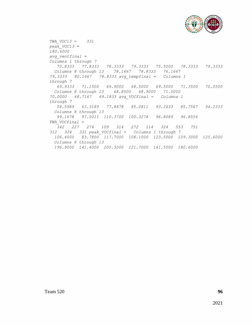
Team 520 96

2021

TWA_VOC13 = 331

peak_VOC13 =

180.6000

avg_ventfinal =

Columns 1 through 7 70.8333 77.8333 78.3333 79.3333 75.5000 78.3333 79.3333 Columns 8 through 13 78.1667 78.8333 76.1667

79.3333 80.1667 78.8333 avg_tempfinal = Columns 1

through 7 69.9333 71.1500 69.9000 68.5000 69.5000 71.3500 70.0500 Columns 8 through 13 68.8500 68.9000 71.5000

70.0000 68.7167 69.1833 avg_VOCfinal = Columns 1

through 7 58.5989 63.3189 77.8878 85.0811 93.2433 85.7567 94.2333 Columns 8 through 13 99.1678 97.0011 110.3700 100.3278 96.8089 96.8556 TWA_VOCfinal = 342 227 274 109 314 272 114 324 553 751

312 324 331 peak_VOCfinal = Columns 1 through 7 106.4000 83.7800 117.7000 108.1000 123.5000 109.3000 125.6000 Columns 8 through 13 196.9000 141.4000 200.3000 121.7000 141.5000 180.6000

Team 520 97

2021

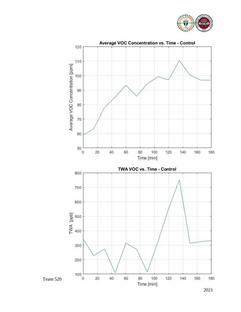
Team 520 98

2021

Team 520 99

2021

Experimental Group (with Acetone)

time = [0:15:180];

% Sample point 1 %


vent_data1e = table2array(Test1day1([1:3,7:9],4))% Importing data

from excel spreadsheet avg_vent1e = mean(vent_data1e)

% Temperature [F] temp_data1e = table2array(Test1day1([1:3,7:9],6))%

Importing data from excel spreadsheet avg_temp1e = mean(temp_data1e)

% VOC [ppm] VOC_data1e = table2array(Test1day1(122:130,9)) %


avg_VOC1e = mean(VOC_data1e) TWA_VOC1e = table2array(Test1day1(122,10))

Team 520 100

2021

peak_VOC1e = table2array(Test1day1(122,12)) % Importing data from

excel spreadsheet

% Sample point 2 %


vent_data2e = table2array(Test1day1([10:12,16:18],4))% Importing

data from excel spreadsheet avg_vent2e = mean(vent_data2e)

% Temperature [F] temp_data2e =


spreadsheet avg_temp2e = mean(temp_data2e)



avg_VOC2e = mean(VOC_data2e) TWA_VOC2e =

table2array(Test1day1(131,10)) peak_VOC2e =


spreadsheet

% Sample point 3 %












spreadsheet


[CFM]

Team 520 101

2021











spreadsheet

% Sample point 5 %












spreadsheet

% Sample point 6 %




% Temperature [F]

temp_data6e = table2array(Test1day1([46:48,52:54],5))% Importing

data from excel spreadsheet avg_temp6e = mean(temp_data6e)

Team 520 102

2021






spreadsheet

% Sample point 7 %












spreadsheet

% Sample point 8 %







% VOC [ppm]

VOC_data8e = table2array(Test1day1(185:193,9)) % Importing data from

excel spreadsheet



Team 520 103

2021


spreadsheet

% Sample point 9 %












spreadsheet

% Sample point 10 %









avg_VOC10e = mean(VOC_data10e) TWA_VOC10e = table2array(Test1day1(203,10))

peak_VOC10e = table2array(Test1day1(203,12)) % Importing data from

excel spreadsheet

% Sample point 11 %


Team 520 104

2021











spreadsheet

% Sample point 12 %


vent_data12e = table2array(Test1day1([100:102,106:108],4))%

Importing data from excel spreadsheet avg_vent12e =

mean(vent_data12e)

% Temperature [F] temp_data12e = table2array(Test1day1([100:102,106:108],6))%

Importing data from excel spreadsheet avg_temp12e =

mean(temp_data12e)






spreadsheet


[CFM]

vent_data13e = table2array(Test1day1([109:111,115:117],4))%

Importing data from excel spreadsheet avg_vent13e =

mean(vent_data13e)

Team 520 105

2021


table2array(Test1day1([109:111,115:117],6))% Importing data from

excel spreadsheet avg_temp13e = mean(temp_data13e)






spreadsheet

% Final Data - Control

avg_ventfinale = [avg_vent1e avg_vent2e avg_vent3e avg_vent4e

avg_vent5e avg_vent6e avg_vent7e avg_vent8e avg_vent9e avg_vent10e

avg_vent11e avg_vent12e avg_vent13e]

avg_tempfinale = [avg_temp1e avg_temp2e avg_temp3e avg_temp4e

avg_temp5e avg_temp6e avg_temp7e avg_temp8e avg_temp9e avg_temp10e

avg_temp11e avg_temp12e avg_temp13e]

avg_VOCfinale = [avg_VOC1e avg_VOC2e avg_VOC3e avg_VOC4e

avg_VOC5e avg_VOC6e avg_VOC7e avg_VOC8e avg_VOC9e avg_VOC10e

avg_VOC11e avg_VOC12e avg_VOC13e] TWA_VOCfinale = [TWA_VOC1e

TWA_VOC2e TWA_VOC3e TWA_VOC4e TWA_VOC5e TWA_VOC6e TWA_VOC7e TWA_VOC8e TWA_VOC9e TWA_VOC10e TWA_VOC11e

TWA_VOC12e TWA_VOC13e] peak_VOCfinale = [peak_VOC1e peak_VOC2e peak_VOC3e peak_VOC4e

peak_VOC5e peak_VOC6e peak_VOC7e peak_VOC8e peak_VOC9e peak_VOC10e

peak_VOC11e peak_VOC12e peak_VOC13e]

figure() % subplot(1,2,1)

plot(time,avg_ventfinale,'.','MarkerSize',8

) grid on xlabel('Time [min]')

ylabel('Average Ventilation Rate [CFM]')

title('Time vs. Average Ventilation Rate')

hold on plot(time,avg_ventfinal,'*')

legend('Experimental','Control','Location','bestoutside'

) figure()

% subplot(1,2,2)

plot(time,avg_tempfinale,'.','MarkerSize',8


ylabel('Average Temperature [F]')

title('Time vs. Average Temperature')

Team 520 106

2021

hold on

plot(time,avg_tempfinal,'*')

legend('Experimental','Control')

% sgtitle('Balometer Data')

figure()

plot(time,avg_VOCfinale,'.','MarkerSize',8


ylabel('Average VOC Concentration [ppm]')

title('Time vs. Average VOC

Concentration')

hold on plot(time,avg_VOCfinal,'*')


)

hold on

plot(0:12) h = yline(80.37, 'b--',

'LineWidth', 1);

legend('Experimental','Control','Experimen

t Mean','Location','bestoutside') figure()

% subplot(1,2,1)

plot(time,TWA_VOCfinale,'.','MarkerSize',8

) grid on xlabel('Time [min]') ylabel('TWA

[ppb]') title('Time vs. TWA VOC')

hold on plot(time,TWA_VOCfinal,'*')


)

figure() % subplot(1,2,2)

plot(time,peak_VOCfinale,'.','MarkerSize',8

) grid on xlabel('Time [min]') ylabel('Peak

VOC Concentration [ppm]') title('Time vs.

Peak VOC Concentration') % sgtitle('VOC

Data')

hold on plot(time,peak_VOCfinal,'*')


) % sgtitle('VOC Data')

vent_data1e

= 75 57 85 78

Team 520 107

2021

69

97

avg_vent1e =

76.8333

temp_data1e

= 71.2000 70.8000 72.4000 72.5000 72.8000 73.2000

avg_temp1e =

72.1500 VOC_data1e = 45.2000 58.5000 53.5000 58.7000 59.2000 46.9000 57.6500 58.3000 61.2000

avg_VOC1e =

55.4611 TWA_VOC1e =

176

peak_VOC1e =

66.1200

vent_data2e

= 79 58 86 83 72

96

avg_vent2e =

79

temp_data2e

= 71.4000 71.2000 71.0000 70.7000 70.4000 70.0000

avg_temp2e =

70.7833 VOC_data2e = 50.7000

Team 520 108

2021

55.7000 75.2000 81.3000 91.7000 69.5000 72.3100 66.9000 66.8000

avg_VOC2e =

70.0122 TWA_VOC2e =

247

peak_VOC2e =

117.2000

vent_data3e

= 77 57 90 79

70

95

avg_vent3e =

78

temp_data3e

= 70.0000 69.8000 70.1000 69.9000 69.7000 70.3000

avg_temp3e =

69.9667 VOC_data3e = 63.8000 71.4000 73.6000 94.7000 112.6000 102.6000 76.8000 114.6000

76.7000

avg_VOC3e =

87.4222 TWA_VOC3e =

291

peak_VOC3e =

159.8000

Team 520 109

2021

vent_data4e

= 75 62 84 79 70 92

avg_vent4e =

77

temp_data4e

= 70.1000 70.4000 69.8000 69.7000 69.8000 70.2000

avg_temp4e =

70 VOC_data4e = 65.8000 71.9000 73.9000 81.5000 94.8000 91.7000 85.6000 94.8000 99.7000

avg_VOC4e =

84.4111 TWA_VOC4e =

275

peak_VOC4e =

126.1000

vent_data5e

= 80 60 88 78 69

94

avg_vent5e =

78.1667

temp_data5e

= 70.1000 70.1000 69.7000 69.9000 70.2000

Team 520 110

2021

70.1000

avg_temp5e =

70.0167 VOC_data5e = 70.0400 73.5000 75.6000 96.4000 100.5000 84.7000 79.9000 95.9000 82.4000

avg_VOC5e =

84.3267 TWA_VOC5e =

298

peak_VOC5e =

164.3000

vent_data6e

= 77 56 86 81

71

99

avg_vent6e =

78.3333

temp_data6e

= 71.3000 71.5000 71.5000 71.4000 71.3000 71.1000

avg_temp6e =

71.3500 VOC_data6e = 109.3000 97.9600 74.0100 78.6700 83.5900 82.0200 77.0000 80.4900 88.7700

avg_VOC6e =

85.7567

Team 520 111

2021

TWA_VOC6e =

272

peak_VOC6e =

109.3000

vent_data7e

= 76 57 84 80 71

98

avg_vent7e =

77.6667

temp_data7e

= 69.9000 70.1000 69.7000 70.1000 69.5000 69.4000

avg_temp7e =

69.7833 VOC_data7e = 59.8000 72.4000 68.7000 80.6000 94.9000 93.6000 103.1000 88.6000 85.5000

avg_VOC7e =

83.0222 TWA_VOC7e =

260

peak_VOC7e =

117

vent_data8e

= 77 57 86 80 71

97

avg_vent8e =

78

temp_data8e

= 68.7000

Team 520 112

2021

69.9000 69.8000 69.6000 69.1000 68.7000

avg_temp8e =

69.3000 VOC_data8e = 60.1000 71.2000 67.3000 97.5000 100.2000 93.1000 89.3000 80.7000 80.5000

avg_VOC8e =

82.2111 TWA_VOC8e = 293

peak_VOC8e =

119.4000

vent_data9e

= 81 60 80 77 70

94

avg_vent9e =

77

temp_data9e

= 69.3000 70.2000 70.1000 69.9000 69.5000 69.1000

avg_temp9e =

69.6833 VOC_data9e = 77.7000 82.2000 84.1000 88.1000 88.3000 76.3000 85.2000

Team 520 113

2021

89.7000 84.1000

avg_VOC9e =

83.9667 TWA_VOC9e =

553

peak_VOC9e =

141.4000

vent_data10e

= 78 59 85 82 72 96

avg_vent10e =

78.6667

temp_data10e

= 69.5000 70.1000 70.2000 69.9000 69.5000 69.1000

avg_temp10e

= 69.7167

VOC_data10e

= 75.4000 83.4000 78.5000 88.0000 87.9000 76.1000 83.2000 89.0000 82.8000

avg_VOC10e =

82.7000 TWA_VOC10e =

510

peak_VOC10e =

136.8000

vent_data11e =

76 57 84 81

69

92

Team 520 114

2021

avg_vent11e =

76.5000

temp_data11e

= 69.9000 70.4000 70.3000 70.2000 70.6000 70.7000

avg_temp11e

= 70.3500 VOC_data11e

= 67.0000 76.0000 69.5000 91.6000 101.0000 94.3000 91.9000 102.1000

88.3000

avg_VOC11e =

86.8556 TWA_VOC11e =

456

peak_VOC11e =

115.9000

vent_data12e =

80 61 88 79

70

94

avg_vent12e =

78.6667

temp_data12e

= 69.7000 69.6000 70.1000 70.2000 70.6000 70.7000

avg_temp12e

= 70.1500 VOC_data12e

= 60.9000

Team 520 115

2021

71.2000 71.7000 85.9000 82.4000 77.8000 93.4000 87.5000 81.7000

avg_VOC12e =

79.1667 TWA_VOC12e =

449

peak_VOC12e =

101.8000

vent_data13e =

78 63 87 82 69 91

avg_vent13e =

78.3333

temp_data13e

= 70.3000 70.5000 70.8000 71.0000 71.2000 71.5000

avg_temp13e

= 70.8833 VOC_data13e

= 61.9000 69.2000 70.3000 79.6000 89.7000 82.7000 85.1000 92.2000 85.1000

avg_VOC13e =

79.5333 TWA_VOC13e = 498

peak_VOC13e =

108.2000

avg_ventfinale =

Columns 1 through 7

Team 520 116

2021

76.8333 79.0000 78.0000 77.0000 78.1667 78.3333 77.6667 Columns 8 through 13 78.0000 77.0000 78.6667

76.5000 78.6667 78.3333 avg_tempfinale = Columns 1

through 7 72.1500 70.7833 69.9667 70.0000 70.0167 71.3500 69.7833 Columns 8 through 13 69.3000 69.6833 69.7167

70.3500 70.1500 70.8833 avg_VOCfinale = Columns 1

through 7 55.4611 70.0122 87.4222 84.4111 84.3267 85.7567 83.0222 Columns 8 through 13 82.2111 83.9667 82.7000 86.8556 79.1667 79.5333 TWA_VOCfinale = 176 247 291 275 298 272 260 293 553 510

456 449 498 peak_VOCfinale = Columns 1 through 7 66.1200 117.2000 159.8000 126.1000 164.3000 109.3000 117.0000 Columns 8 through 13 119.4000 141.4000 136.8000 115.9000 101.8000 108.2000

Team 520 117

2021

Team 520 118

2021

Team 520 119

2021

Published with MATLAB® R2021a

Team 520 120

2021

Appendix G: Risk Assessment

Name of Project: Trane: Improve Air Quality &

Efficiency

Date of submission: 12/4/20

Team member Phone number Email

Jake Hamilton (321) 427-2803 [email protected]

Nicholas Holm (954) 732-2503 [email protected]

Andreu Santeiro (305) 484-5947 [email protected]

Joseph Thyer (850) 510-6575 [email protected]

Gavin Young (727) 453-8563 [email protected]

Faculty mentor Phone number Email

Dr. Shayne McConomy (850) 410-6624 [email protected]

Dr. Juan Ordonez (850)-644-8405 [email protected]

Rewrite the project steps to include all safety measures taken for each step or combination of

steps. Be specific (don’t just state “be careful”).

The ionization unit utilized high voltage. Testers will wear insulating gloves and rubber soled shoes.

The device will always be checked for residual charge before being handled.

The tested air flow will contain small particulate. Testers will wear respiratory masks and safety

goggles. The testing apparatus will be carefully designed to contain the particulate and air flow.

Organic growth will be tested. Testers will wear respiratory masks, safety goggles, and gloves. The

testing apparatus will be carefully designed to contain mold and bacterial growth.

A testing apparatus will be constructed or assembled. Sharp edges may present themselves during

construction. Testers will wear long sleeves and long pants, close toed shoes, and gloves.

OSHA regulations were checked in regard to personnel safety when working with high voltage and

small particulate.

Thinking about the accidents that have occurred or that you have identified as a risk, describe

emergency response procedures to use.

Assess the victim and the scene. If necessary, call the local emergency number to activate the EMS

system. If the victim is conscious, ask for permission to provide care. Provide required care or wait for

proper care providers.

List emergency response contact information:

• Call 911 for injuries, fires or other emergency situations

• Call your department representative to report a facility concern

Name Phone number Faculty emergency contact Phone number

Fire Department (850) 891-6600 Dr. Shayne McConomy (850) 410-6624

Bruce Thyer (850) 508-8880 Dr. Juan Ordonez (850)-644-8405

Donald Hollett (850) 410-6600

Team 520 121

2021

Safety review signatures

Team member Date Faculty mentor Date

Jake Hamilton 12/1/20 Dr. Shayne McConomy 12/1/20

Nicholas Holm 12/1/20 Dr. Juan Ordonez 12/1/20

Andreu Santeiro 12/1/20

Joseph Thyer 12/1/20

Gavin Young 12/1/20

Report all accidents and near misses to the faculty mentor.

References

Air Quality. (2019, December 24). Retrieved October 15, 2020,

from https://morpc.gohio.com/commute-resources/air-quality/

Corson, S., & Vargas, M. (2020, August 19). TRANE: Indoor Air Quality (IAQ)- Related

HVAC Guidance from ASHRAE® and the CDC. Retrieved October 13, 2020.

Drozdov, M. (2020, September 29). How to manage indoor air quality amid covid-19.

Retrieved March 30, 2021, from https://www.randrmagonline.com/articles/89119-how-to-

manage-indoor-air-quality-amid-covid-19

Fredrich, L., McDowell, J., Ponczak, G., Tanzilo, B., & Tarnoff, A. (1970, March 06).

When will it feel safe to go back indoors? Retrieved March 30, 2021,

from https://onmilwaukee.com/articles/indoor-air-quality

Hanania, J. (2018, September). Energy Education: Electrostatic precipitator.

Retrieved November 13, 2020, from https://energyeducation.ca/encyclopedia/Electrostatic_preci

pitator

https://morpc.gohio.com/commute-resources/air-quality/



https://www.randrmagonline.com/articles/89119-how-to-manage-indoor-air-quality-amid-covid-19

https://www.randrmagonline.com/articles/89119-how-to-manage-indoor-air-quality-amid-covid-19

https://onmilwaukee.com/articles/indoor-air-quality

https://energyeducation.ca/encyclopedia/Electrostatic_precipitator

https://energyeducation.ca/encyclopedia/Electrostatic_precipitator

Team 520 122

2021

Housh, W. (2020, February 28). Mold in HVAC System: Clean HVAC Ductwork:

HVAC.com®. Retrieved January 18, 2021, from https://www.hvac.com/blog/what-are-the-

effects-of-mold-in-my-hvac-system-and-how-do-i-know-if-i-have-it/

Lafond, A. (2018, September 26). Threshold limit values of volatile organic compounds.

Retrieved March 30, 2021, from https://foobot.io/guides/threshold-limit-values-volatile-organic-

compounds.php

Lee, S., Hyun, J., Lee, S., & Hwang, J. (2013, December 21). One-pass antibacterial

efficacy of Bipolar AIR Ions against AEROSOLIZED Staphylococcus epidermidis in a duct

flow. Retrieved February 25, 2021, from

https://www.sciencedirect.com/science/article/pii/S0021850213002516

Lower, A. (2020, November). Will a higher MERV filter affect my airflow?

Retrieved November 10, 2020, from https://www.secondnature.com/blog/higher-merv-air-filter-

affect-air-flow

Marsden, J., & Fink, R. (2020, May). Hydro-Peroxide for Indoor Air Quality.

Retrieved November 10, 2020, from https://www.rgf.com/article/hydro-peroxide-for-iaq/

MIT. (2020, June 23). Covid-19 Updates. Retrieved January 19, 2021,

from https://medical.mit.edu/covid-19-updates/2020/09/air-conditioning-risks

Pappas, S. (2020, March 31). Coronavirus testing is ramping up. Here are the new tests

and how they work. Retrieved January 20, 2021, from https://www.livescience.com/coronavirus-

tests-available.html

https://www.hvac.com/blog/what-are-the-effects-of-mold-in-my-hvac-system-and-how-do-i-know-if-i-have-it/

https://www.hvac.com/blog/what-are-the-effects-of-mold-in-my-hvac-system-and-how-do-i-know-if-i-have-it/

https://foobot.io/guides/threshold-limit-values-volatile-organic-compounds.php

https://foobot.io/guides/threshold-limit-values-volatile-organic-compounds.php


https://www.secondnature.com/blog/higher-merv-air-filter-affect-air-flow

https://www.secondnature.com/blog/higher-merv-air-filter-affect-air-flow

https://www.rgf.com/article/hydro-peroxide-for-iaq/

https://medical.mit.edu/covid-19-updates/2020/09/air-conditioning-risks%E2%80%8B

https://medical.mit.edu/covid-19-updates/2020/09/air-conditioning-risks%E2%80%8B

https://www.livescience.com/coronavirus-tests-available.html

https://www.livescience.com/coronavirus-tests-available.html

Team 520 123

2021

Partners, N. (n.d.). Photohydroionization™ (PHI) - an ADVANCED Oxidation

Technology. Retrieved March 30, 2021,

from https://newportpartnersllc.com/technologies/hvac/photohydroionization.html

Rich, S. (2011, October 3). IT Projects Improve Air Quality, Receive Grant Funding.

Retrieved January 18, 2021, from https://www.govtech.com/budget-finance/IT-Projects-

Improve-Air-Quality-Receive-Grant-Funding.html

Steiner, G., & Reischl, G. (2012, July 23). The effect of carrier gas contaminants on the

charging probability of aerosols under bipolar charging conditions. Retrieved March 18, 2021,

from https://www.sciencedirect.com/science/article/pii/S0021850212001334

https://newportpartnersllc.com/technologies/hvac/photohydroionization.html

https://www.govtech.com/budget-finance/IT-Projects-Improve-Air-Quality-Receive-Grant-Funding.html

https://www.govtech.com/budget-finance/IT-Projects-Improve-Air-Quality-Receive-Grant-Funding.html


Team 520: Trane: Improve Air Quality

Documents

Transcript of Team 520: Trane: Improve Air Quality