NBER WORKING PAPER SERIES

TEACHER PERFORMANCE PAY:EXPERIMENTAL EVIDENCE FROM INDIA

Karthik MuralidharanVenkatesh Sundararaman

Working Paper 15323http://www.nber.org/papers/w15323

NATIONAL BUREAU OF ECONOMIC RESEARCH1050 Massachusetts Avenue

Cambridge, MA 02138September 2009

We are grateful to Caroline Hoxby, Michael Kremer, and Michelle Riboud for their support, advice,and encouragement at all stages of this project. We thank George Baker, Efraim Benmelech, Eli Berman,Damon Clark, Julie Cullen, Gordon Dahl, Jishnu Das, Martin Feldstein, Richard Freeman, RobertGibbons, Edward Glaeser, Roger Gordon, Gordon Hanson, Richard Holden, Asim Khwaja, DavidLevine, Jens Ludwig, Sendhil Mullainathan, Ben Olken, Lant Pritchett, Halsey Rogers, Richard Romano,Kartini Shastry, Jeff Williamson, and various seminar participants for useful comments and discussions.This paper is based on a project known as the Andhra Pradesh Randomized Evaluation Study (APRESt), which is a partnership between the Government of Andhra Pradesh, the Azim Premji Foundation,and the World Bank. Financial assistance for the project has been provided by the Government ofAndhra Pradesh, the UK Department for International Development (DFID), the Azim Premji Foundation,and the World Bank. We thank Dileep Ranjekar, Amit Dar, Samuel C. Carlson, and officials of theDepartment of School Education in Andhra Pradesh (particularly Dr. I.V. Subba Rao, Dr. P. Krishnaiah,K. Ramakrishna Rao, and Suresh Chanda), for their continuous support and long-term vision for thisresearch. We are especially grateful to DD Karopady, M Srinivasa Rao, and staff of the Azim PremjiFoundation for their leadership and meticulous work in implementing this project. Sridhar Rajagopalan,Vyjyanthi Shankar, and staff of Educational Initiatives led the test design. We thank Vinayak Alladi,Gokul Madhavan, Ketki Sheth and Maheshwor Shrestha for outstanding research assistance. The findings,interpretations, and conclusions expressed in this paper are those of the authors and do not necessarilyrepresent the views of the World Bank, its Executive Directors, the governments they represent, orthe National Bureau of Economic Research.

NBER working papers are circulated for discussion and comment purposes. They have not been peer-reviewed or been subject to the review by the NBER Board of Directors that accompanies officialNBER publications.

© 2009 by Karthik Muralidharan and Venkatesh Sundararaman. All rights reserved. Short sectionsof text, not to exceed two paragraphs, may be quoted without explicit permission provided that fullcredit, including © notice, is given to the source.

Teacher Performance Pay: Experimental Evidence from IndiaKarthik Muralidharan and Venkatesh SundararamanNBER Working Paper No. 15323September 2009JEL No. C93,I21,M52,O15

ABSTRACT

Performance pay for teachers is frequently suggested as a way of improving education outcomes inschools, but the theoretical predictions regarding its effectiveness are ambiguous and the empiricalevidence to date is limited and mixed. We present results from a randomized evaluation of a teacherincentive program implemented across a large representative sample of government-run rural primaryschools in the Indian state of Andhra Pradesh. The program provided bonus payments to teachers basedon the average improvement of their students' test scores in independently administered learning assessments(with a mean bonus of 3% of annual pay). At the end of two years of the program, students in incentiveschools performed significantly better than those in control schools by 0.28 and 0.16 standard deviationsin math and language tests respectively. They scored significantly higher on "conceptual" as well as"mechanical" components of the tests, suggesting that the gains in test scores represented an actualincrease in learning outcomes. Incentive schools also performed better on subjects for which therewere no incentives, suggesting positive spillovers. Group and individual incentive schools performedequally well in the first year of the program, but the individual incentive schools outperformed in thesecond year. Incentive schools performed significantly better than other randomly-chosen schoolsthat received additional schooling inputs of a similar value.

Karthik MuralidharanDepartment of Economics, 0508University of California, San Diego9500 Gilman DriveLa Jolla, CA 92093-0508and NBERkamurali@ucsd.edu

Venkatesh SundararamanSouth Asia Human Development UnitThe World Bank1818 H Street, NWWashington, DC 20433 vsundararaman@worldbank.org

- 1 -

1. Introduction A fundamental question in education policy around the world is that of the relative

effectiveness of input-based and incentive-based policies in improving the quality of schools.

While the traditional approach to improving schools has focused on providing them with more

resources, there has been growing interest in directly measuring and incentivizing schools and

teachers based on student learning outcomes.1 The idea of paying teachers based on direct

measures of performance has attracted particular attention since teacher salaries are the largest

component of education budgets and recent research shows that teacher characteristics rewarded

under the status quo in most school systems (such as experience and master’s degrees in

education) are poor predictors of better student outcomes.2

However, while the idea of using incentive pay schemes for teachers as a way of improving

school performance is increasingly making its way into policy,

3 the empirical evidence on the

effectiveness of such policies is quite limited – with identification of the causal impact of teacher

incentives being the main challenge. In addition, several studies have highlighted the possibility

of perverse outcomes resulting from high-powered teacher incentives,4

In this paper, we contribute towards filling this gap with evidence from a large-scale

randomized evaluation of a teacher performance pay program implemented in the Indian state of

Andhra Pradesh (AP). We studied two types of teacher performance pay (group bonuses based

on school performance, and individual bonuses based on teacher performance), with the average

bonus calibrated to be around 3% of a typical teacher’s annual salary. The incentive program

was designed to minimize the likelihood of undesired consequences (see design details later) and

suggesting the need for

caution and better evidence before expanding teacher incentive programs based on test scores.

1 This shift in emphasis can be attributed at least in part to the several studies that have pointed to the low correlations between school spending and learning outcomes (see Hanushek (2006) for a review). The “No Child Left Behind” Act of 2001 (NCLB) formalized education policy focus on learning outcomes in the US. Of course, inputs and incentives are not mutually exclusive, but the distinction has policy salience in terms of the relative importance given to the two kinds of approaches, starting from the current status quo. 2 See Rivkin, Hanushek, and Kain (2005), Rockoff (2004), and Gordon, Kane, and Staiger (2006) 3 Teacher performance pay is being considered and implemented in several US states including Colorado, Florida, Tennessee, and Texas, and additional resources have been dedicated to a Federal “Teacher Incentive Fund” by the US Department of Education in 2009. International examples of attempts to tie teacher pay to performance include the UK, Israel, Chile, and Australia. 4 Examples of sub-optimal behavior by teachers include rote 'teaching to the test' and neglecting higher-order skills (Holmstrom and Milgrom, 1991), manipulating performance by short-term strategies like boosting the caloric content of meals on the day of the test (Figlio and Winicki, 2005), excluding weak students from testing (Jacob, 2005), focusing only on some students in response to "threshold effects" embodied in the structure of the incentives (Neal and Schanzenbach, 2008) or even outright cheating (Jacob and Levitt, 2003).

- 2 -

the study was conducted by randomly allocating the incentive programs across a representative

sample of 300 government-run schools in rural AP with 100 schools each in the group and

individual incentive treatment groups and 100 schools serving as the comparison group.5

We find no evidence of any adverse consequences as a result of the incentive programs.

Incentive schools do significantly better on both mechanical components of the test (designed to

reflect rote learning) and conceptual components of the test (designed to capture deeper

understanding of the material),

This large-scale experiment allows us to answer a comprehensive set of questions with

regard to teacher performance pay including: (i) Can teacher performance pay based on test

scores improve student achievement? (ii) What, if any, are the negative consequences of teacher

incentives based on student test scores? (iii) How do school-level group incentives compare with

teacher-level individual incentives? (iv) How does teacher behavior change in response to

performance pay? and (v) How cost effective are teacher incentives relative to other uses for the

same money?

We find that the teacher performance pay program was highly effective in improving student

learning. At the end of two years of the program, students in incentive schools performed

significantly better than those in comparison schools by 0.28 and 0.16 standard deviations (SD)

in math and language tests respectively. The mean treatment effect of 0.22 SD is equal to 9

percentile points at the median of a normal distribution. We find a minimum average treatment

effect of 0.1 SD at every percentile of baseline test scores, suggesting broad-based gains in test

scores as a result of the incentive program.

6

5 The program was implemented by the Azim Premji Foundation (a leading non-profit organization working to improve primary education in India) on behalf of the Government of Andhra Pradesh, with technical support from the World Bank. These interventions were part of a larger project called the AP RESt (Andhra Pradesh Randomized Evaluation Study) that aimed to rigorously evaluate the impact of several policy options to improve the quality of primary education in AP. We have served as technical consultants and have overseen the design, and evaluation of the various interventions. 6 We engaged India’s leading education testing firm (“Education Initiatives”) to design the tests to our specifications so that we could directly test for crowding out of higher-order skills under a performance pay program for teachers.

suggesting that the gains in test scores represent an actual

increase in learning outcomes. Students in incentive schools do significantly better not only in

math and language (for which there were incentives), but also in science and social studies (for

which there were no incentives), suggesting positive spillover effects. There was no difference

in student attrition between incentive and control schools, and no evidence of any adverse

gaming of the incentive program by teachers.

- 3 -

School-level group incentives and teacher-level individual incentives perform equally well in

the first year of the program, but the individual incentive schools significantly outperformed the

group incentive schools in the second year. At the end of two years, the average treatment effect

was 0.27 SD in the individual incentive schools compared to 0.16 SD in the group incentive

schools, with this difference being nearly significant at the 10% level.

We measure changes in teacher behavior in response to the program with both teacher

interviews as well as direct physical observation of teacher activity. Our results suggest that the

main mechanism for the impact of the incentive program was not increased teacher attendance,

but greater (and more effective) teaching effort conditional on being present.

We find that performance-based bonus payments to teachers were a significantly more cost

effective way of increasing student test scores compared to spending a similar amount of money

unconditionally on additional schooling inputs. In a parallel initiative, two other sets of 100

randomly-chosen schools were provided with an extra contract teacher, and with a cash grant for

school materials respectively.7

There was broad-based support from teachers for the program, and we also find that the

extent of teachers' ex-ante support for performance pay (over a series of mean-preserving spreads

of pay) is positively correlated with their ex-post performance. This suggests that teachers are

aware of their own effectiveness and that performance pay might not only increase effort among

existing teachers, but systematically draw more effective teachers into the profession over time.

At the end of two years, students in schools receiving the input

programs scored 0.08 SD higher than those in comparison schools. However, the incentive

programs had a significantly larger impact on learning outcomes (0.22 versus 0.08 SD) over the

same period, even though the total cost of the bonuses was around 25% lower than the amount

spent on the inputs.

8

Our results contribute to a small but growing literature on the effectiveness of performance-

based pay for teachers.

9

7 The details of the input interventions and their impact on learning outcomes are in companion papers (Muralidharan and Sundararaman (2009), and Das et al (2009)), but the summary of the input program effects are discussed in this paper to enable the comparison between inputs and incentives. 8 Lazear (2000) shows that around half the gains from performance-pay in the company he studied were due to more productive workers being attracted to join the company under a performance-pay system. Similarly, Hoxby and Leigh (2005) argue that compression of teacher wages in the US is an important reason for the decline in teacher quality, with higher-ability teachers exiting the teacher labor market.

The best identified studies on the effect of paying teachers on the basis

9Previous studies include Ladd (1999) in Dallas, Atkinson et al (2004) in the UK, and Figlio and Kenny (2007) who use cross-sectional data across multiple US states. Duflo, Hanna, and Ryan (2007) present an experimental evaluation of a program that provided incentives to teachers based on attendance. See Umansky (2005) and

- 4 -

of student test outcomes are Lavy (2002) and (2008), and Glewwe, Ilias, and Kremer (2008), but

their evidence is mixed. Lavy uses a combination of regression discontinuity, difference in

differences, and matching methods to show that both group and individual incentives for high

school teachers in Israel led to improvements in student outcomes (in the 2002 and 2008 papers

respectively). Glewwe et al (2008) report results from a randomized evaluation that provided

primary school teachers (grades 4 to 8) in Kenya with group incentives based on test scores and

find that, while test scores went up in program schools in the short run, the students did not retain

the gains after the incentive program ended. They interpret these results as being consistent with

teachers expending effort towards short-term increases in test scores but not towards long-term

learning.10

There are several unique features in the design of the field experiment presented in this

paper. We conduct the first randomized evaluation of teacher performance pay in a

representative sample of schools.

11

While set in the context of schools and teachers, this paper also contributes to the broader

literature on performance pay in organizations in general and public organizations in particular.

We take incentive theory seriously and design the incentive

program to minimize the risk of perverse outcomes, and design the study to test for a wide range

of possible negative outcomes. We study group (school-level) and individual (teacher-level)

incentives in the same field experiment. We measure changes in teacher behavior with both

direct observations and with teacher interviews. Finally, we study both input and incentive based

policies in the same field experiment to enable a direct comparison of their effectiveness.

12

True experiments in compensation structure with contemporaneous control groups are rare,13

Podgursky and Springer (2007) for reviews on teacher performance pay and incentives. The term "teacher incentives" is used very broadly in the literature. We use the term to refer to financial bonus payments on the basis of student test scores. 10 It is worth nothing though that evidence from several contexts and interventions suggests that the effect of almost all education interventions appear to decay when the programs are discontinued (see Jacob et al, 2008, and Andrabi et al, 2008), and so this inference should be qualified. 11 The random assignment of treatment provides high internal validity, while the random sampling of schools into the universe of the study provides greater external validity than typical experiments by avoiding the “randomization bias”, whereby entities that are in the experiment are atypical relative to the population that the result is sought to be extrapolated to (Heckman and Smith (1995)). 12 See Gibbons (1998) and Prendergast (1999) for general overviews of the theory and empirics of incentives in organizations. Dixit (2002) provides a discussion of these themes as they apply to public organizations. Chiappori and Salanié (2003) survey recent empirical work in contract theory and emphasize the identification problems in testing incentive theory. 13 Bandiera, Barankay, and Rasul (2007) is a recent exception that studies the impact of exogenously varied compensation schemes (though with a sequential as opposed to contemporaneous comparison group).

and

- 5 -

our results may be relevant to answering broader questions regarding performance pay in

organizations.14

2.1 Incentives and intrinsic motivation

The rest of this paper is organized as follows: section 2 provides a theoretical framework for

thinking about teacher incentives. Section 3 describes the experimental design and the

treatments, while section 4 discusses the test design. Sections 5 and 6 present results on the

impact of the incentive programs on test score outcomes and teacher behavior. Section 7

discusses the cost effectiveness of the performance-pay programs, while section 8 discusses

teacher responsiveness to the idea of performance pay. Section 9 concludes.

2. Theoretical Framework

It is not obvious that paying teachers bonuses on the basis of student test scores will even

raise test scores. Evidence from psychological studies suggests that monetary incentives can

sometimes crowd out intrinsic motivation and lead to inferior outcomes.15 Teaching may be

especially susceptible to this concern since many teachers are thought to enter the profession due

to strong intrinsic motivation. The AP context, however, suggested that an equally valid concern

was the lack of differentiation among high and low-performing teachers. Kremer et al (2005)

show that in Indian government schools, teachers reporting high levels of job satisfaction are

more likely to be absent. In subsequent focus group discussions with teachers, it was suggested

that this was because teachers who were able to get by with low effort were quite satisfied, while

hard-working teachers were dissatisfied because there was no difference in professional

outcomes between them and those who shirked. Thus, it is also possible that the lack of external

reinforcement for performance can erode intrinsic motivation.16

In summary, the psychological literature on incentives suggests that extrinsic incentives that

are perceived by workers as a means of exercising control over them are more likely to crowd

out intrinsic motivation, while those that are seen as reinforcing norms of professional behavior

14 Of course, as Dixit (2002) warns, it is important for empirical work to be cautious in making generalizations about performance-based incentives, and to focus on relating success or failure of incentive pay to context-specific characteristics such as the extent and nature of multi-tasking. 15 A classic reference in psychology is Deci and Ryan (1985). Fehr and Falk (2002) survey the psychological foundations of incentives and their relevance for economics. Chapter 5 of Baron and Kreps (1999) provides a good discussion relating intrinsic motivation to practical incentive design and communication. 16 Mullainathan (2006) describes how high initial intrinsic motivation of teachers can diminish over time if they feel that the government does not appreciate or reciprocate their efforts.

- 6 -

can enhance intrinsic motivation (Fehr and Falk, 2002). Thus, the way an incentive program is

framed can influence its effectiveness. The program studied here was careful to frame the

incentives in terms of “recognition” of excellence in teaching as opposed to framing the program

in terms of “school and teacher accountability”.

2.2 Multi-task moral hazard

Even those who agree that incentives based on test scores could improve test performance

worry that such incentives could lead to sub-optimal behavioral responses from teachers.

Examples of such behavior include rote 'teaching to the test' and neglecting higher-order skills

(Holmstrom and Milgrom, 1991), manipulating performance by short-term strategies like

boosting the caloric content of meals on the day of the test (Figlio and Winicki, 2005), excluding

weak students from testing (Jacob, 2005), focusing on some students to the exclusion of others in

response to “threshold effects” embodied in the incentive design (Neal and Schanzenbach, 2008)

or even outright cheating (Jacob and Levitt, 2003).

These are all examples of the problem of multi-task moral hazard, which is illustrated by the

following formulation from Baker (2002).17 a Let be an n-dimensional vector of potential agent

(teacher) actions that map into a risk-neutral principal's (social planner's) value function (V)

through a linear production function of the form:

εε +⋅= afa ),(V

where f is a vector of marginal products of each action on V, and ε is noise in V.

Assume the principal can observe V (but not a) and offers a linear wage contract of the form

Vbsw v ⋅+= . If the agent's expected utility is given by:

∑=

−⋅+⋅−⋅+n

iivv aVbshVbsE

1

2 2/)var()(

where h is her coefficient of absolute risk aversion and 2/2ia is the cost of each action, then the

optimal slope on output ( *vb ) is given by:

22

2*

2 εσhFFbv +

= (2.2.1)

17 The original references are Holmstrom and Milgrom (1991), and Baker (1992). The treatment here follows Baker (2002) which motivates the multi-tasking discussion by focusing on the divergence between the performance measure and the principal's objective function.

- 7 -

where ∑ ==

n

i ifF1

2 . Expression (2.2.1) reflects the standard trade-off between risk and

aligning of incentives, with the optimal slope *vb decreasing as h and 2

εσ increase.

Now, consider the case where the principal cannot observe V but can only observe a

performance measure (P) that is also a linear function of the action vector a given by:

φφ +⋅= aga ),(P

Since g ≠ f, P is an imperfect proxy for V (such as test scores for broader learning). However,

since V is unobservable, the principal is constrained to offer a wage contract as a function of P

such as Pbsw p ⋅+= .

The key result in Baker (2002) is that the optimal slope *pb on P is given by:

22*

2cos

φσθ

hGGFbp +⋅⋅

= (2.2.2)

where ∑==

n

i igG1

2 , and θ is the angle between f and g. The cosine of θ is a measure of how

much *pb needs to be reduced relative to *

vb due to the distortion arising from g ≠ f.

The empirical literature in education showing that teachers sometimes respond to incentives

by increasing actions on dimensions that are not valued by the principal highlights the need to be

cautious in designing incentive programs. In most practical cases, g ≠ f (and cos 1θ ≠ ), and so

it is perhaps inevitable that a wage contract with 0>pb will induce some actions that are

unproductive. However, what matters for incentive design is that 0* >pb , as long as

))0(())0(( =>> pp bVbV aa , even if there is some deviation relative to the first-best action in the

absence of distortion and )(())(( **vp bVbV aa < . In other words, what matters is not whether

teachers engage in more or less of some activity than they would in a first-best world (with

incentives on the underlying social value function), but whether the sum of their activities in a

system with incentives on test scores generates more learning (broadly construed) than in a

situation with no such incentives.

There are several reasons why test scores might be an adequate performance measure in the

context of primary education in a developing country. First, given the extremely low levels of

learning, it is likely that even an increase in routine classroom teaching of basic material will

- 8 -

lead to better learning outcomes.18 Second, even if some of the gains merely reflect an

improvement in test-taking skills, the fact that the education system in India (and several Asian

countries) is largely structured around test-taking suggests that it might be unfair to deny

disadvantaged children in government-schools the benefits of test-taking skills that their more

privileged counterparts in private schools develop.19

2.3 Group versus Individual Incentives

Finally, the design of tests can get more

sophisticated over time, making it difficult to do well on the tests without a deeper understanding

of the subject matter. So, it is possible that additional efforts taken by teachers to improve test

scores for primary school children can also lead to improvements in broader educational

outcomes. Whether this is true is an empirical question and is a focus of our research design (see

section 4).

The theoretical prediction of the relative effectiveness of individual and group teacher

incentives is ambiguous. To clarify the issues, let w = wage, P = performance measure, and c(a)

= cost of exerting effort a with c'(a) > 0, c''(a) > 0, P'(a) > 0, and P''(a) < 0. Unlike typical cases

of team production, an individual teacher's output (test scores of his students) is observable,

making contracts on individual output feasible. The optimal effort for a teacher facing individual

incentives is to choose ai so that: i i

i i

w PP a

∂ ∂⋅ =

∂ ∂ c'(ai) (2.3.1)

Now, consider a group incentive program where the bonus payment is a function of the

average performance of all teachers. The optimality condition for each teacher is:

( )( )i ii

ii i

P P nwaP P n

−

−

∂ +∂ ⋅ =∂ ∂ +

∑∑

c'(ai) (2.3.2)

If the same bonus is paid to a teacher for a unit of performance under both group and

individual incentives then ( )

i i

ii i

w wPP P n−

∂ ∂=∂ ∂ + ∑

, but ( ) 1i i i

i i

P P n Pa n a

− ∂ + ∂ = ⋅

∂ ∂∑

. Since

c''(a) > 0, the equilibrium effort exerted by each teacher under group incentives is lower than that

18 As Lazear (2006) points out, the optimal policy regarding high-stakes tests are different for high-cost and low-cost learners, with concentrated incentives being optimal for high-cost learners. This would be analogous to saying that teaching to the test may be optimal in contexts of very low learning. 19 While the private returns to test-taking skills may be greater than the social returns, the social returns could be positive if they enable disadvantaged students to compete on a more even basis with privileged students for scarce slots in higher levels of education.

- 9 -

under individual incentives. Thus, in the basic theory, group (school-level) incentives induce

free riding and are therefore inferior to individual (teacher-level) incentives, when the latter are

feasible.20

However, if the teachers jointly choose their effort levels, they will account for the

externalities within the group. In the simple case where they each have the same cost and

production functions and these functions do not depend on the actions of the other teachers, they

will each (jointly) choose the level of effort given by (2.3.1). Of course, each teacher has an

incentive to shirk relative to this first best effort level, but if teachers in the school can monitor

each other at low cost, then it is possible that the same level of effort can be implemented as

under individual incentives. This is especially applicable to smaller schools where peer

monitoring is likely to be easier.

21

Finally, if there are gains to cooperation or complementarities in production, then it is

possible that group incentives might yield better results than individual incentives.

22

( )a∀

Consider a

case where teachers have comparative advantages in teaching different subjects or different types

of students. If teachers specialize in their area of advantage and reallocate students/subjects to

reflect this, they could raise P'(a) relative to a situation where each teacher had to teach all

students/subjects. Since P''(a) < 0, the equilibrium effort would also be higher and the outcomes

under group incentives could be superior to those under individual incentives.23

Lavy (2002) and (2008) report results from high-school teacher incentive programs in Israel

at the individual and group level respectively. However, the two programs were implemented at

different (non-overlapping) times and the schools were chosen by different (non-random)

eligibility criteria, and the individual incentive program was only studied for one year. We study

both group and individual incentives in the same field experiment over two full academic years.

20 See Holmstrom (1982) for a solution to the problem of moral hazard in teams. 21 See Kandori (1992) and Kandel and Lazear (1992) for discussions of how social norms and peer pressure in groups can ensure community enforcement of the first best effort level. 22 Itoh (1991) models incentive design when cooperation is important. Hamilton, Nickerson, and Owan (2003) present empirical evidence from a garment factory showing that group incentives for workers improved productivity relative to individual incentives. 23 The additive separability of utility between income and cost of effort implies that there is no 'income effect' of higher productivity on the cost of effort, and so effort goes up in equilibrium since P'(a) is higher.

- 10 -

3. Experimental Design 3.1 Context

While India has made substantial progress in improving access to primary schooling and

primary school enrolment rates, the average levels of learning remain very low. The most recent

Annual Status of Education Report found that over 58% of children aged 6 to 14 in an all-India

sample of over 300,000 rural households could not read at the second grade level, though over

95% of them were enrolled in school (Pratham, 2008). Public spending on education has been

rising as part of the “Education for All” campaign, but there are substantial inefficiencies in

public delivery of education services. A recent study using a nationally representative dataset of

primary schools in India found that 25% of teachers were absent on any given day, and that less

than half of them were engaged in any teaching activity (Kremer et al (2005)).24

The average rural primary school is quite small, with total enrollment of around 80 to 100

students and an average of 3 teachers across grades one through five.

Andhra Pradesh (AP) is the 5th most populous state in India, with a population of over 80

million, 73% of whom live in rural areas. AP is close to the all-India average on measures of

human development such as gross enrollment in primary school, literacy, and infant mortality, as

well as on measures of service delivery such as teacher absence (Figure 1a). The state consists

of three historically distinct socio-cultural regions and a total of 23 districts (Figure 1b). Each

district is divided into three to five divisions, and each division is composed of ten to fifteen

mandals, which are the lowest administrative tier of the government of AP. A typical mandal

has around 25 villages and 40 to 60 government primary schools. There are a total of over

60,000 such schools in AP and over 80% of children in rural AP attend government-run schools

(Pratham, 2008).

25

24 Spending on teacher salaries and benefits comprises over 90% of non-capital spending on education in India. 25 This is a consequence of the priority placed on providing all children with access to a primary school within a distance of 1 kilometer from their homes.

One teacher typically

teaches all subjects for a given grade (and often teaches more than one grade simultaneously).

All regular teachers are employed by the state, and their salary is mostly determined by

experience and rank, with minor adjustments based on assignment location, but no component

based on any measure of performance. The average salary of regular teachers is over Rs.

8,000/month and total compensation including benefits is close to Rs. 10,000/month (per capita

- 11 -

income in AP is around Rs. 2,000/month; 1 US Dollar ≈ 48 Indian Rupees (Rs.)). Teacher

unions are strong and disciplinary action for non-performance is rare.26

3.2 Sampling

We sampled 5 districts across each of the 3 socio-cultural regions of AP in proportion to

population (Figure 1b).27

3.3 AP RESt Design Overview

In each of the 5 districts, we randomly selected one division and then

randomly sampled 10 mandals in the selected division. In each of the 50 mandals, we randomly

sampled 10 schools using probability proportional to enrollment. Thus, the universe of 500

schools in the study was representative of the schooling conditions of the typical child attending

a government-run primary school in rural AP.

The overall design of AP RESt is represented in the table below:

Table 3.1

NONE GROUP BONUS

INDIVIDUAL BONUS

NONE CONTROL (100 Schools) 100 Schools 100 Schools

EXTRA CONTRACT TEACHER 100 Schools

EXTRA BLOCK GRANT 100 Schools

INCENTIVES (Conditional on Improvement in Student Learning

INPUTS (Unconditional)

As Table 3.1 shows, the input treatments (described in section 7) were provided unconditionally

to the selected schools at the beginning of the school year, while the incentive treatments

consisted of an announcement that bonuses would be paid at the beginning of the next school

year conditional on average improvements in test scores during the current school year. No

school received more than one treatment, which allows the treatments to be analyzed

independent of each other. The school year in AP starts in the middle of June, and the baseline

26 See Kingdon and Muzammil (2001) for an illustrative case study of the power of teacher unions in India. Kremer et al (2005) find that 25% of teachers are absent across India, but only 1 head teacher in their sample of 3000 government schools had ever fired a teacher for repeated absence. 27 The districts were chosen so that districts within a region would be contiguous for ease of logistics and program implementation.

- 12 -

tests were conducted in the 500 sampled schools during late June and early July, 2005.28

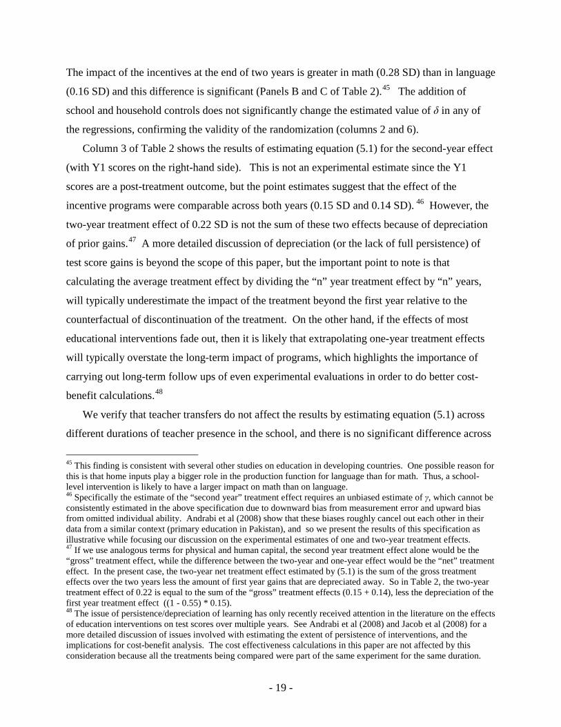
Table 1 (Panel A) shows summary statistics of baseline school and student performance

variables by treatment (control schools are also referred to as a 'treatment' for expositional ease).

Column 4 provides the p-value of the joint test of equality, showing that the null of equality

across treatment groups cannot be rejected for any of the variables and that the randomization

worked properly.

After

the baseline tests were scored, 2 out of the 10 project schools in each mandal were randomly

allocated to each of 5 cells (four treatments and one control). Since 50 mandals were chosen

across 5 districts, there were a total of 100 schools (spread out across the state) in each cell. The

geographic stratification implies that every mandal was an exact microcosm of the overall study,

which allows us to estimate the treatment impact with mandal-level fixed effects and thereby net

out any common factors at the lowest administrative level of government.

29

After the randomization, mandal coordinators (MCs) from APF personally went to each of

the schools in the first week of August 2005 to provide them with student, class, and school

performance reports, and with oral and written communication about the intervention that the

school was receiving. The MCs also made several rounds of unannounced tracking surveys to

each of the schools during the school year to collect data on process variables including student

attendance, teacher attendance and activity, and classroom observation of teaching processes.

30

End of year assessments were conducted in March and April, 2006 in all project schools.

The results were provided to the schools in the beginning of the next school year (July – August,

All schools operated under identical conditions of information and monitoring and only differed

in the treatment that they received. This ensures that Hawthorne effects are minimized and that a

comparison between treatment and control schools can accurately isolate the treatment effect.

28 See Appendix A for the project timeline and activities and Appendix B for details on test administration. The selected schools were informed by the government that an external assessment of learning would take place in this period, but there was no communication to any school about any of the treatments at this time (since that could have led to gaming of the baseline test). 29 Table 1 shows sample balance across control, group incentive, and individual incentive schools, which are the focus of the analysis in this paper. The randomization was done jointly across all 5 treatments shown in Table 3.1, and the sample was also balanced on observables across the other treatments. 30 Six visits were made to each school in the first year (2005 – 06), while four visits were made in the second year (2006 – 07)

- 13 -

2006), and all schools were informed that the program would continue for another year.31

3.4 Description of Incentive Treatments

Bonus

checks based on first year performance were sent to qualifying teachers by the end of September

2006, following which the same processes were repeated for a second year.

Teachers in incentive schools were offered bonus payments on the basis of the average

improvement in test scores (in math and language) of students taught by them subject to a

minimum improvement of 5%. The bonus formula was:

Bonus = Rs. 500 * (% Gain in average test scores – 5%) if Gain > 5%

= 0 otherwise32

All teachers in group incentive schools received the same bonus based on average school-level

improvement in test scores, while the bonus for teachers in individual incentive schools was

based on the average test score improvement of students taught by the specific teacher. We use a

(piecewise) linear formula for the bonus contract, both for ease of communication and

implementation and also because it is the most resistant to gaming across periods (the end of year

score in any year determines the target score for the subsequent year).

33

The 'slope' of Rs. 500 per percentage point gain in average scores was set so that the

expected incentive payment per school would be approximately equal to the additional spending

in the input treatments (based on calibrations from the project pilot).

34

31 The communication to teachers with respect to the length of the program was that the program would continue as long as the government continued to support the project. The expectation conveyed to teachers during the first year was that the program was likely to continue but was not guaranteed to do so. 32 1st grade students were not tested in the baseline, and so their ‘target’ score for a bonus (above which the linear schedule above would apply) was set to be the mean baseline score of the 2nd grade students in the school. The target for the 2nd grade students was equal to their baseline score plus the 5% threshold described above. Schools selected for the incentive programs were given detailed letters and verbal communications explaining the incentive formula. Sample communication letters are available from the authors on request. 33 Holmstrom and Milgrom (1987) show the theoretical optimality of linear contracts in a dynamic setting (under assumptions of exponential utility for the agent and normally distributed noise). Oyer (1998) provides empirical evidence of gaming in response to non-linear incentive schemes. 34 The best way to set expected incentive payments to be exactly equal to Rs. 10,000/school would have been to run a tournament with pre-determined prize amounts. Our main reason for using a contract as opposed to a tournament was that contracts were more transparent to the schools in our experiment since the universe of eligible schools was spread out across the state. Individual contracts (without relative performance measurement) also dominate tournaments for risk-averse agents when specific shocks (at the school or class level) are more salient for the outcome measure than aggregate shocks (across all schools), which is probably the case here (see Kane and Staiger, 2002). See Lazear and Rosen (1981) and Green and Stokey (1983) for a discussion of tournaments and when they dominate contracts.

The threshold of 5%

average improvement was introduced to account for the fact that the baseline tests were in

- 14 -

June/July and the end of year tests would be in March/April, and so the baseline score might be

artificially low due to students forgetting material over the summer vacation. There was no

minimum threshold in the second year of the program because the first year's end of year score

was used as the second year's baseline and the testing was conducted at the same time of the

school year on a 12-month cycle.35

We tried to minimize potentially undesirable 'threshold' effects, where teachers only focus on

students near a performance target, by making the bonus payment a function of the average

improvement of all students.

36 If the function transforming teacher effort into test-score gains is

concave (convex) in the baseline score, teachers would have an incentive to focus on weaker

(stronger) students, but no student is likely to be wholly neglected since each contributes to the

class average. In order to discourage teachers from excluding students with weak gains from

taking the end of year test, we assigned a zero improvement score to any child who took the

baseline test but not the end of year test.37 To make cheating as difficult as possible, the tests

were conducted by external teams of 5 evaluators in each school (1 for each grade), the identity

of the students taking the test was verified, and the grading was done at a supervised central

location at the end of each day's testing (see Appendix B for details).38

35 The convexity in reward schedule in the first year due to the threshold could have induced some gaming, but the distribution of mean class and school-level gains at the end of the first year of the program did not have a gap below the threshold of 5%. If there is no penalty for a reduction in scores, there is convexity in the payment schedule even if there is no threshold (at a gain of zero). To reduce the incentives for gaming in subsequent years, we use the higher of the baseline and year end scores as the target for the next year and so a school/class whose performance deteriorates does not have its target reduced for the next year. 36 Many of the negative consequences of incentives discussed in Jacob (2005) are a response to the threshold effects created by the targets in the program he studied. Neal and Schanzenbach (2008) discuss the impact of threshold effects in the No Child Left Behind act on teacher behavior and show that teachers do in fact focus more on students on the ‘bubble’ and relatively neglect students far above or below the thresholds. We anticipated this concern and designed the incentive schedule accordingly. 37 In the second year (when there was no threshold), students who took the test at the end of year 1 but not at the end of year 2 were assigned a score of -5. Thus, the cost of a dropping out student to the teacher was always equal to a negative 5% score for the student concerned. A higher penalty would have been difficult since most cases of attrition are out of the teacher’s control. The penalty of 5% was judged to be adequate to avoid explicit gaming of the test taking population. We also cap negative gains at the student-level at -5% for the calculation of teacher bonuses. Thus, putting a floor on the extent to which a poor performing student brought down the class/school average at -5% ensured that a teacher/school could never do worse than having a student drop out to eliminate any incentive to get weak students to not appear for the test. 38 There were no cases of cheating in the first year, but two cases of cheating were detected in the second year (one classroom and one entire school). These cases were reported to the project management team by the field enumerators, and the concerned schools/teachers were subsequently disqualified from receiving any bonus for the second year. These cases are not included in the analysis presented in the paper.

- 15 -

4. Test Design 4.1 Test Construction

We engaged India's leading education testing firm, "Educational Initiatives" (EI), to design

the tests to our specifications. The test design activities included mapping the syllabus from the

text books into skills, creating a universe of questions to represent each skill, and calibrating

question difficulty in a pilot exercise in 40 schools during the prior school year (2004-05) to

ensure adequate discrimination on the tests.

The baseline test (June-July, 2005) covered competencies up to that of the previous school

year. At the end of the school year (March-April, 2006), schools had two rounds of tests with a

gap of two weeks between them. The first test (referred to as the “lower end line” or LEL)

covered competencies up to that of the previous school year, while the second test (referred to as

the “higher end line” or HEL) covered materials from the current school year's syllabus. The

same procedure was repeated at the end of the second year, with two rounds of testing.39 Doing

two rounds of testing at the end of each year allows for the inclusion of more overlapping

materials across years of testing, reduces the impact of measurement errors specific to the day of

testing by having multiple tests around two weeks apart, and also reduces sample attrition due to

student absence on the day of the test.40

4.2 Basic versus higher-order skills

For the rest of this paper, Year 0 (Y0) refers to the baseline tests in June-July 2005; Year 1

(Y1) refers to both rounds of tests conducted at the end of the first year of the program in March-

April, 2006; and Year 2 (Y2) refers to both rounds of tests conducted at the end of the second

year of the program in March-April, 2007.

As highlighted in section 2.2, it is possible that broader educational outcomes are no better

(or even worse) under a system of teacher incentives based on test scores even if the test scores

improve. A key empirical question, therefore, is whether additional efforts taken by teachers to

improve test scores for primary school children in response to the incentives are also likely to 39 Thus in any year of testing, the materials in the LEL will overlap with those on the HEL the previous year. This makes it possible to put student achievement over time on a common “vertical scale” using the properties of item response theory (IRT), which is the standard psychometric tool used to equate different tests on a common scale (the IRT estimates are not used in this paper). 40 Since all analysis is done with normalized test scores (relative to the control school distribution), a student can be absent on one testing day and still be included in the analysis without bias because the included score would have been normalized relative to the specific test that the student took.

- 16 -

lead to improvements in broader educational outcomes. We asked EI to design the tests to

include both 'mechanical' and 'conceptual' questions within each skill category on the test. The

distinction between these two categories is not constant, since a conceptual question that is

repeatedly taught in class can become a mechanical one. Similarly a question that is conceptual

in an early grade might become mechanical in a later grade, if students acclimatize to the idea

over time. For this study, a mechanical question was considered to be one that conformed to the

format of the standard exercises in the text book, whereas a conceptual one was defined as a

question that tested the same underlying knowledge or skill in an unfamiliar way.

As an example, consider the following pair of questions (which did not appear sequentially)

from the 4th grade math test under the skill of 'multiplication and division'

The first question follows the standard textbook format for asking multiplication questions

and would be classified as "mechanical" while the second one requires the students to understand

that the concept of multiplication is that of repeated addition, and would be classified as

"conceptual." Note that conceptual questions are not more difficult per se. In this example, the

conceptual question is arguably easier than the mechanical one because a student only has to

count that there are 6 '8's and enter the answer '6' as opposed to multiplying 2 numbers with a

digit carried forward. But the conceptual question is unfamiliar and this is reflected in 43% of

children getting Question 1 correct, while only 8% got Question 2 correct. Of course, the

distinction is not always so stark, and the classification into mechanical and conceptual is a

discrete representation of a continuous scale between familiar and unfamiliar questions.41

4.3 Incentive versus non-incentive subjects

Another dimension on which incentives can induce distortions is on the margin between

incentive and non-incentive subjects. We study the extent to which this is a problem by

conducting additional tests at the end of each year in science and social studies on which there

41 Koretz (2002) points out that test score gains are only meaningful if they generalize from the specific test to other indicators of mastery of the domain in question. While there is no easy solution to this problem given the impracticality of assessing every domain beyond the test, our inclusion of both mechanical and conceptual questions in each test attempts to address this concern.

Question 1: 34 x 5

Question 2: Put the correct number in the empty box: 8 + 8 + 8 + 8 + 8 + 8 = 8 x

- 17 -

was no incentive.42

Since these subjects are introduced only in grade 3 in the school curriculum,

these additional tests were administered in grades 3 to 5.

5. Results 5.1 Teacher Turnover and Student Attrition

Regular civil-service teachers in AP are transferred once every three years on average.

While this could potentially bias our results if more teachers chose to stay in or tried to transfer

into the incentive schools, it is unlikely that this was the case since the treatments were

announced in August ’05, while the transfer process typically starts earlier in the year. There

was no statistically significant difference between any of the treatment groups in the extent of

teacher turnover or attrition, and the transfer rate was close to 33%, which is consistent with the

rotation of teachers once every 3 years (Table 1 – Panel B, rows 11-12). A more worrying

possibility was that additional teachers would try to transfer into the incentive schools in the

second year of the project. As part of the agreement between the Government of AP and the

Azim Premji Foundation, the Government agreed to minimize transfers into and out of the

sample schools for the duration of the study. The average teacher turnover in the second year

was only 5%, and once again, there was no significant difference in teacher transfer rates across

the various treatments (Table 1 – Panel B, rows 13 - 16).43

The average student attrition rate in the sample (defined as the fraction of students in the

baseline tests who did not take a test at the end of each year) was 7.3% and 25% in year 1 and

year 2 respectively, but there is no significant difference in attrition across the treatments (rows

17 and 20). Beyond confirming sample balance, this is an important result in its own right

because one of the concerns of teacher incentives based on test scores is that weaker children

might be induced to drop out of testing in incentive schools (Jacob, 2005). Attrition is higher

among students with lower baseline scores, but this is true across all treatments, and we find no

42 In the first year of the project, schools were not told about these additional subject tests till a week prior to the tests and were told that these tests were only for research purposes. In the second year, the schools knew that these additional tests would be conducted, but also knew from the first year that these tests would not be included in the bonus calculations. 43 There was also a court order to restrict teacher transfers in response to litigation complaining that teacher transfers during the school year were disruptive to students. This may have also helped to reduce teacher transfers during the second year of the project.

- 18 -

significant difference in mean baseline test score across treatment categories among the students

who drop out from the test-taking sample (Table 1 – Panel B, rows 18, 19, 21, 22).

5.2 Specification

We first discuss the impact of the incentive program as a whole by pooling the group and

individual incentive schools and considering this to be the 'incentive' treatment. All estimation

and inference is done with the sample of 300 control and incentive schools unless stated

otherwise. Our default specification uses the form:

ijkjkkmijkmnijkm ZIncentivesYTYT εεεβδγα +++⋅+⋅+⋅+= )()( 0 (5.1)

The main dependent variable of interest is ijkmT , which is the normalized test score on the

specific test (normalized with respect to the score distribution of the control schools), where i, j,

k, m denote the student, grade, school, and mandal respectively. 0Y indicates the baseline tests,

while nY indicates a test at the end of n years of the program. Including the normalized baseline

test score improves efficiency due to the autocorrelation between test-scores across multiple

periods.44

5.3 Impact of Incentives on Test Scores

All regressions include a set of mandal-level dummies (Zm) and the standard errors are

clustered at the school level. Since the treatments are stratified by mandal, including mandal

fixed effects increases the efficiency of the estimate. We also run the regressions with and

without controls for household and school variables.

The 'Incentives' variable is a dummy at the school level indicating if it was in the incentive

treatment, and the parameter of interest is δ, which is the effect on the normalized test scores of

being in an incentive school. The random assignment of treatment ensures that the 'Incentives'

variable in the equation above is not correlated with the error term, and the estimate of the one-

year and two-year treatment effects are therefore unbiased.

Averaging across both math and language, students in incentive schools scored 0.15 standard

deviations (SD) higher than those in comparison schools at the end of the first year of the

program, and 0.22 SD higher at the end of the second year (Table 2 – Panel A, columns 1 and 5).

44 Since grade 1 students did not have a baseline test, we set the normalized baseline score to zero for these students (similarly for students in grade 2 at the end of two years of the treatment). All results are robust to completely excluding grade 1 students as well.

- 19 -

The impact of the incentives at the end of two years is greater in math (0.28 SD) than in language

(0.16 SD) and this difference is significant (Panels B and C of Table 2).45

Column 3 of Table 2 shows the results of estimating equation (5.1) for the second-year effect

(with Y1 scores on the right-hand side). This is not an experimental estimate since the Y1

scores are a post-treatment outcome, but the point estimates suggest that the effect of the

incentive programs were comparable across both years (0.15 SD and 0.14 SD).

The addition of

school and household controls does not significantly change the estimated value of δ in any of

the regressions, confirming the validity of the randomization (columns 2 and 6).

46 However, the

two-year treatment effect of 0.22 SD is not the sum of these two effects because of depreciation

of prior gains.47 A more detailed discussion of depreciation (or the lack of full persistence) of

test score gains is beyond the scope of this paper, but the important point to note is that

calculating the average treatment effect by dividing the “n” year treatment effect by “n” years,

will typically underestimate the impact of the treatment beyond the first year relative to the

counterfactual of discontinuation of the treatment. On the other hand, if the effects of most

educational interventions fade out, then it is likely that extrapolating one-year treatment effects

will typically overstate the long-term impact of programs, which highlights the importance of

carrying out long-term follow ups of even experimental evaluations in order to do better cost-

benefit calculations.48

We verify that teacher transfers do not affect the results by estimating equation (5.1) across

different durations of teacher presence in the school, and there is no significant difference across

45 This finding is consistent with several other studies on education in developing countries. One possible reason for this is that home inputs play a bigger role in the production function for language than for math. Thus, a school-level intervention is likely to have a larger impact on math than on language. 46 Specifically the estimate of the “second year” treatment effect requires an unbiased estimate of γ, which cannot be consistently estimated in the above specification due to downward bias from measurement error and upward bias from omitted individual ability. Andrabi et al (2008) show that these biases roughly cancel out each other in their data from a similar context (primary education in Pakistan), and so we present the results of this specification as illustrative while focusing our discussion on the experimental estimates of one and two-year treatment effects. 47 If we use analogous terms for physical and human capital, the second year treatment effect alone would be the “gross” treatment effect, while the difference between the two-year and one-year effect would be the “net” treatment effect. In the present case, the two-year net treatment effect estimated by (5.1) is the sum of the gross treatment effects over the two years less the amount of first year gains that are depreciated away. So in Table 2, the two-year treatment effect of 0.22 is equal to the sum of the “gross” treatment effects (0.15 + 0.14), less the depreciation of the first year treatment effect ((1 - 0.55) * 0.15). 48 The issue of persistence/depreciation of learning has only recently received attention in the literature on the effects of education interventions on test scores over multiple years. See Andrabi et al (2008) and Jacob et al (2008) for a more detailed discussion of issues involved with estimating the extent of persistence of interventions, and the implications for cost-benefit analysis. The cost effectiveness calculations in this paper are not affected by this consideration because all the treatments being compared were part of the same experiment for the same duration.

- 20 -

these estimates. The testing process was externally proctored at all stages and we had no reason

to believe that cheating was a problem in the first year, but there were two cases of cheating in

the second year. Both these cases were dropped from the analysis and the concerned

schools/teachers were declared ineligible for bonuses (see Appendix B).

The top panel of Figure 2 plots the density and CDF of the test score distribution in treatment

and control schools at the baseline and the lower panel plots them after two years of the program.

Figure 3 plots the quantile treatment effects of the performance pay program on student test

scores (defined for each quantileτ as: )()()( 11 τττδ −− −= mn FG where nG and mF represent the

empirical distributions of the treatment and control distributions with n and m observations

respectively), with bootstrapped 95% confidence intervals, and shows that the quantile treatment

effects are positive at every percentile and increasing. In other words, test scores in incentive

schools are higher at every percentile, but the program also increased the variance of test scores.

5.4 Heterogeneity of Treatment Effects

We find that students in incentive schools do better than control schools for all major sub-

groups including all five grades (1-5), all five project districts, both rounds of testing (lower end

line and higher end line), and across all quintiles of question difficulty, with most of these

differences being significant (since the sample size is large enough to precisely estimate

treatment effects in various sub-groups).49

3δ

We test for heterogeneity of the incentive treatment effect across student, school, and teacher

characteristics by testing if is significantly different from zero in:

sticCharacteriIncentivesYTYT ijkmnijkm ⋅+⋅+⋅+= 210 )()( δδγα

ijkjkkmZsticCharacteriIncentives εεεβδ +++⋅+×⋅+ )(3 (5.2)

Table 5 (Panel A) shows the results of these regressions on several school and household

characteristics.50

49 These tables are not included in the paper, but are available from the authors on request. 50 Each column in Table 3 represents one regression testing for heterogeneous treatment effects along the characteristic mentioned. We also estimate the heterogeneity non-parametrically for each non-binary characteristic, grouping the characteristic into quintiles, and testing if the interaction of the incentive treatment and the top or bottom quintile is significantly different from the omitted category (the middle 3 quintiles), and if the interaction of the incentive treatment with the top and bottom quintiles are significantly different from each other. The results are unchanged and so the table only reports the linear interaction specification in (5.2).

We find very limited evidence of differential treatment effects by school

characteristics such as total number of students, school infrastructure, or school proximity to

- 21 -

facilities. 51

The lack of heterogeneous treatment effects by baseline score is an important indicator of

broad-based gains since the baseline score is probably the best summary statistic of prior inputs

into education. To see this more clearly, Figure 4 shows the non-parametric treatment effects by

baseline score,

We also find no evidence of a significant difference in the effect of the incentives by

most of the student demographic variables, including an index of household literacy, the caste of

the household, the student's gender, and the student's baseline score. The only evidence of

heterogeneous treatment effects is across levels of family affluence, with students from more

affluent families showing a better response to the teacher incentive program.

52 and we see that there is a minimum treatment effect of 0.1 SD for students

regardless of where they were in the initial test score distribution.53

51 Given the presence of several covariates in Table 3, we are cautious to avoid data mining for differential treatment effects since a few significant coefficients are likely simply due to sampling variability. Thus, we consider consistent evidence of heterogeneous treatment effects across multiple years to be more reliable evidence. 52 The figure plots a kernel-weighted local polynomial regression of end line scores (after 2 years) on baseline scores separately for the incentive and control schools, and also plots the difference at each percentile of baseline scores. The confidence intervals of the treatment effects are constructed by drawing 1000 bootstrap samples of data that preserve the within school correlation structure in the original data, and plotting the 95% range for the treatment effect at each percentile of baseline scores. 53 We are thus able to test for the “bubble” student effect found in studies of NCLB such as Neal and Schanzenbach (2008) and can rule out the presence of a similar effect here.

The treatment effects are

slightly lower for students with higher baseline scores, but this is not a significant trend as seen

in Column 8 of Table 3 (Panel A).

The lack of heterogeneous treatment effects by initial scores, suggests that the increase in

variance of test scores in incentive schools (Figure 3) may be reflecting variance in teacher

responsiveness to the incentive program, as opposed to variance in student responsiveness to the

treatment by initial learning levels. We test this by estimating teacher value addition (measured

as teacher fixed effects in a regression of current test scores on lagged scores) and find that both

the mean and variance of teacher value-addition are significantly higher in the incentive schools

(Figure 5). Plotting the difference in teacher fixed effects at each percentile of the control and

treatment distribution shows the heterogeneity in teacher responsiveness quite clearly. We see

that there is no difference between treatment and control schools for the bottom 20% of teachers

(as measured by their effectiveness in increasing student test scores); the difference between the

20th and 60th percentile is positive but with a 5% confidence bound that is close to zero; and

finally the difference between the 60th and 100th percentile is positive, significant, and increasing.

- 22 -

Having established that there is variation in teacher responsiveness to the incentive program,

we test for differential responsiveness by observable teacher characteristics (Table 3B). We find

that the interaction of teachers’ education and training with incentives is positive and significant,

while education and training by themselves are not significant predictors of value addition. This

suggests that teacher qualifications by themselves are not associated with better learning

outcomes under the status quo, they could matter more if teachers had incentives to exert more

effort (see Hanushek (2006)).

We also find that teachers with higher base pay respond less well to the incentives (Table 3 –

Panel B, column 4), which suggests that the magnitude of the incentive mattered because the

potential incentive amount (for which all teachers had the same conditions) would have been a

larger share of base pay for lower paid teachers. However, teachers with higher base pay are

typically more experienced and we see that more experienced teachers also respond less well to

the incentives (column 3). So, while this evidence suggests that the magnitude of the bonus

matters, it is also consistent with an interpretation that young teachers respond better to any new

policy initiative (including performance pay), and so we cannot distinguish the impact of the

incentive amount from that of other teacher characteristics that influence base pay.54

5.5 Mechanical versus Conceptual Learning and Non-Incentive Subjects

To test the impact of incentives on these two kinds of learning, we again use specification

(5.1) but run separate regressions for the mechanical and conceptual parts of the test. Incentive

schools do significantly better on both the mechanical and conceptual components of the test and

the estimate of δ is almost identical across both components (Table 4). Note that the coefficient

on the baseline score is significantly lower for the conceptual component than for the mechanical

component (in both years), indicating that these questions were more unfamiliar than the

mechanical questions. The relative unfamiliarity of these questions increases our confidence that

the gains in test scores represent genuine improvements in learning outcomes.

The impact of incentives on the performance in non-incentive subjects such as science and

social studies is tested using a slightly modified version of specification (5.1) where lagged

scores on both math and language are included to control for initial learning levels. We find that

students in incentive schools also performed significantly better on non-incentive subjects at the 54 Of course, this is a caution that applies to any interpretation of interactions in an experiment, since the covariate is not randomly assigned and could be correlated with other omitted variables.

- 23 -

end of each year of the program, scoring 0.11 and 0.18 SD higher than students in control

schools in science and social studies at the end of two years of the program (Table 5). The

coefficients on the lagged baseline math and language scores here are much lower than those in

Tables 2 and 4, confirming that the domain of these tests was substantially different from that of

the tests on which incentives were paid.

These results do not imply that no diversion of teacher effort away from science, social

studies, or conceptual thinking took place, but rather that in the context of primary education in a

developing country with very low levels of learning, teacher efforts aimed at increasing test

scores in math and language are also likely to contribute to superior performance on broader

educational outcomes suggesting complementarities among the measures and positive spillover

effects between them (though the result could also be due to an improvement in test-taking skills

that transfer across subjects).

5.6 Group versus Individual Incentives

Both the group and the individual incentive programs had significantly positive treatment

effects at the end of each year of the program (Table 6, columns 1 and 7).55

We find no significant impact of the number of teachers in the school on the relative

performance of group and individual incentives (both linear and quadratic interactions of school

size with the group incentive treatment are insignificant). However, the variation in school size

is small with 92% of group incentive schools having between two and five teachers (the mean

number of teachers across the 300 schools was 3.28, the median was 3, and the mode was 2).

The limited range of school size makes it difficult to precisely estimate the impact of group size

on the relative effectiveness of group incentives.

In the first year of

the program, students in individual incentive schools performed slightly better than those in

group incentive schools, but the difference was not significant. By the end of the second year,

students in individual incentive schools scored 0.27 SD higher than those in comparison schools,

while those in group incentive schools scored 0.16 SD higher, with this difference being close to

significant at the 10% level (column 7). Estimates of the treatment effect in the second year

alone (column 4) suggest that individual incentive schools significantly outperformed group

incentive schools in the second year.

55 Table 6 is estimated with specification (5.1) but separating out the “incentive” treatment into group and individual incentives respectively.

- 24 -

We repeat all the analysis presented above (in sections 5.3 – 5.5) after separating the

incentive schools into the group and individual incentive categories, and Table 7 shows the

disaggregated effect of group and individual incentives for each grade, for

mechanical/conceptual questions, and for science and social studies. We find that the individual

incentives always outperform the group incentives though the difference in point estimates are

typically not significant. However, both individual and group incentives were equally cost

effective, because the bonuses paid were a function of student performance (see section 7). We

also find no significant difference in the patterns of heterogeneous treatment effects (discussed in

the previous section) between individual and group incentive schools.

6. Teacher Behavior and Classroom Processes A unique feature of this study is that changes in teacher behavior were measured with both

direct observation as well as teacher interviews. As described in section 3.3, APF staff

enumerators conducted several rounds of unannounced tracking surveys during the two school

years across all schools in the project. The enumerators coded teacher activity (and absence)

through direct physical observation of each teacher in the school. To code classroom processes,

an enumerator typically spent between 20 and 30 minutes at the back of a classroom (during each

visit) without disturbing the class and coded whether specific actions took place during the

period of observation. In addition to these observations, they also interviewed teachers about

their teaching practices and methods, asking identical sets of questions in both incentive and

control schools. These interviews were conducted in August 2006, around 4 months after the

end of year tests, but before any results were announced, and a similar set of interviews was

conducted in August 2007 after the second full year of the program.

There was no difference in either student or teacher attendance between control and incentive

schools. We also find no significant difference between incentive and control schools on any of

the various indicators of classroom processes as measured by direct observation.56

56 These include measures of teacher activity such as using the blackboard, reading from the textbook, asking questions to students, encouraging classroom participation, assigning homework, helping students individually, and measures of student activity such as using textbooks, and asking questions.

This is

similar to the results in Glewwe et al (2003) who find no difference in teacher behavior between

treatment and control schools from similar surveys and raises the question of how the outcomes

- 25 -

are significantly different when there don't appear to be any differences in observed processes

between the schools.

The teacher interviews provide another way of testing for differences in behavior. Teachers

in both incentive and control schools were asked unprompted questions about what they did

differently during the school year at the end of each school year, but before they knew the results

of their students. The interviews indicate that teachers in incentive schools are significantly

more likely to have assigned more homework and class work, conducted extra classes beyond

regular school hours, given practice tests, and paid special attention to weaker children (Table 8).

While self-reported measures of teacher activity might be considered less credible than

observations, we find a positive and significant correlation between nearly all the reported

activities of teachers and the performance of their students (Table 8 – column 4) suggesting that

these self-reports were credible (especially since less than 50% of teachers in the incentive

schools report doing any of the activities described in Table 8).

The interview responses suggest reasons for why salient dimensions of changes in teacher

behavior might not have been captured in the classroom observations. An enumerator sitting in

classrooms during the school day is unlikely to observe the extra classes conducted after school.

Similarly, if the increase in practice tests occurred closer to the end of the school year (in

March), this would not have been picked up by the tracking surveys conducted between

September and February. Finally, while our survey instruments recorded if various activities

took place, they did not have a way to capture the intensity of teacher efforts, which may be an

important channel of impact. One way to see this is to notice that there is no difference between

treatment and control schools in the fraction of teachers coded as “actively teaching” when

observed by the enumerator (Table 8 – row 2), but the interaction of “active teaching” and being

in an incentive school is significantly positively correlated with measures of teacher value

addition (Table 3B – column 7). This suggests that teachers changed the effectiveness of their

teaching in response to the incentives in ways that would not be easily captured even by

observing the teacher.

Our use of both direct observations and interviews might help in reconciling the difference

between the findings of Glewwe et al. (2008) and Lavy (2008) with respect to teacher behavior.

Glewwe et al. use direct observation and report that there was no significant difference in teacher

actions between incentive and comparison schools; Lavy uses phone interviews with teachers

- 26 -

and reports that teachers in incentive schools were significantly more likely to conduct extra

classes, stream students by ability, and provide extra help to weak students. While both methods

are imperfect, our results suggest that the difference between the studies could partly be due to

the different methodologies used for measuring classroom process variables. In summary, it

appears that the incentive program based on end of year test scores did not change the teachers'

cost-benefit calculations on the presence/absence margin on a given day during the school year,

but that it probably made them exert more effort when present (especially closer to the end of

year assessments).

7. Comparison with Input Treatments & Cost-Benefit Analysis As mentioned earlier, a parallel component of this study provided two other sets of 100

randomly chosen schools with an extra contract teacher, and with a cash block grant for school

materials respectively. Contract teachers are hired at the school level and have usually

completed either high school or college, but typically have no formal teacher training. Their

contracts are renewed annually and they are not protected by any civil-service rules. Their

typical salary is less than 20% of the average salary of regular government teachers. Contract

teachers usually teach their own classes and are not 'teacher-aides' who support a regular teacher

in the same classroom. The use of contract teachers has increased in developing countries like

India in response to fiscal pressures and to the difficulty of filling teacher positions in under-

served remote areas. There is some evidence that contract teachers are more cost effective than

regular teachers but their use is controversial. Proponents argue that contract teachers are a cost-

effective way of reducing class size and multi-grade teaching; opponents argue that the use of

untrained teachers will not improve learning.57

The block grant intervention targeted non-teacher inputs directly used by students. The

schools had the freedom to decide how to spend the block grant, subject to guidelines that

required the money to be spent on inputs directly used by children. Schools receiving the block

grant were given a few weeks to make a list of items they would like to procure. The list was

approved by the project manager, and the materials were jointly procured by the teachers and the

APF mandal coordinators, and provided to the schools by September, 2005. The majority of the

57 See our companion paper (Muralidharan and Sundararaman, 2009) for more details on the program and its impact on student learning.

- 27 -

grant money was spent on notebooks, workbooks, exercise books, slates and chalk, writing

materials, and other interactive materials such as charts, maps, and toys.58

These interventions were calibrated so that the expected spending on the input and the

incentive programs was roughly equal.

59

ijkjkkmijkmnijkm ZInputsIncentivesYTYT εεεβδδγα +++⋅+⋅+⋅+⋅+= 210 )()(

To compare the effects across treatment types, we pool

the 2 incentive treatments, the 2 input treatments, and the control schools and run the regression:

(7.1)

using the full sample of 500 schools. While both categories of treatments had a positive and

significant impact on learning outcomes at the end of the first year, the incentive schools

performed 0.06 standard deviations better than the input schools and this difference is significant

at the 10 percent level (Table 9 - Column 1). At the end of two years, the difference is more

pronounced with the incentive schools scoring 0.13 SD higher and this difference is significant at

the 1% level (Table 9 – Column 7). The incentive schools perform better than input schools in

both math and language and both these differences are significant at the end of two years.

The total amount spent on each intervention was calibrated to be roughly equal, but the group

incentive program ended up spending significantly lower amounts per school. The average

annual spending on each of the input treatments was Rs. 10,000/school, while the group and

individual incentives programs cost roughly Rs. 6,000/school and Rs.10,000/school respectively.

The bonus payment in the group incentive schools was lower than that in the individual incentive

schools both because the treatment effect was smaller and also because classes with scores below

their target brought down the average school gain in the group incentive schools, while teachers

with negative gains (relative to targets) did not hurt teachers with positive gains in the individual

incentive schools.60

Both the incentive programs were more cost effective than the input programs. The

individual incentive program spent the same amount per school as the input programs but

produced gains in test scores that were three times larger than those in the input schools (0.27 SD

58 See Das et al (2009), where we discuss the impact of the block grant intervention. 59 These input programs represented 2 out of the 3 most common input-based interventions (infrastructure, teachers, and materials). We did not conduct a randomized evaluation of infrastructure both due to practical difficulties, and because the returns would have to be evaluated over the depreciation life cycle of the infrastructure. Thus, the set of interventions studied here all represent “flow” expenditures that would be incurred annually and are therefore comparable. 60 So even conditional on the same distribution of scores, the individual incentive payout would be higher as long as there are some classes with negative gains relative to the target because of truncation of teacher-level bonuses at zero in the individual incentive calculations.

- 28 -

vs. 0.09 SD). The group incentive program had a smaller treatment effect than the individual

incentive program (0.16 SD vs 0.27 SD), but on a cost effectiveness basis the group and

individual incentive programs were almost identical in their effectiveness (0.16 SD for Rs. 6,000

in the group incentive schools and 0.27 SD for Rs. 10,000 in the individual incentive schools).

Thus, both the incentive programs significantly outperformed the input programs and were

roughly equal to each other in cost effectiveness.

A different way of thinking about the cost of the incentive program is to not consider the

incentive payments as a cost at all, because it is simply a way of reallocating salary spending.

For instance, if salaries were increased by 3% every year for inflation, then it might be possible

to introduce a performance-based component with an expected payout of 3% of base pay in lieu

of a standard increase across the board. Under this scenario, the 'incentive cost' would only be

the risk premium needed to keep expected utility constant compared to the guaranteed increase

of 3%. This is a very small number with an upper bound of 0.1% of base pay if teachers'

coefficient of absolute risk aversion (CARA) is 2 and 0.22% of base pay even if the CARA is as

high 5.61 This is less than 10% of the mean incentive payment (3% of base pay) and thus, the

long-run cost of the incentive program can be substantially lower than the full cost of the

bonuses paid in the short run.62

A full discussion of cost effectiveness should include an estimate of the cost of administering

the program. The main cost outside the incentive payments is that of independently

administering and grading the tests. The approximate cost of each annual round of testing was

Rs. 5,000 per school, which includes the cost of two rounds of independent testing and data entry

Finally, if performance-pay programs are designed on the basis

of multiple years of performance, differences in compensation across teachers would be less due

to random variation (which would need to be compensated for by paying a risk-premium), and

more due to heterogeneity in ability, which would attract higher-ability teachers into the

profession, and reduce the rents paid to less effective teachers (see next section).

61 The risk premium here is the value of ε such that )()]03.1()97.0([5.0 wuwuwu =+++ εε , and is easily estimated for various values of CARA using a Taylor expansion around w. This is a conservative upper bound since the incentive program is modeled as an even lottery between the extreme outcomes of a bonus of 0% and 6%. In practice, the support of the incentive distribution would be non-zero everywhere on [0, 6] and the risk premium would be considerably lower. 62 This would not be true for the current teachers in the system who are used to low levels of effort, and who would need to be compensated not only for the risk of variable pay but for the extra effort that they may need to exert under a performance-pay system. However, new teachers who are not accustomed to the rents of the civil-service job would only need to be compensated for the risk premium.

- 29 -

but not the additional costs borne for research purposes. The incentive program would be more

cost effective than the input programs even after adding these costs and even more so if we take

the long-run view that the fiscal cost of performance pay can be lower than the amount of the

bonus, if implemented in lieu of a scheduled across the board increase in pay.

8. Teacher Opinions on Performance Pay

Nearly 75% of teachers in incentive schools report that their motivation levels went up as a

result of the program (with the other 25% reporting no change); over 95% had a favorable

opinion about the program; over 85% had a favorable opinion regarding the idea of providing

bonus payments to teachers on the basis of performance; and over two thirds of teachers felt that

the government should consider implementing a system of bonus payments on the basis of

performance.

Of course, it is easy to support a program when it only offers rewards and no penalties, and

so we also asked the teachers their opinion regarding performance-pay in an expected wage-

neutral way. Teachers were asked their preference regarding how they would allocate a

hypothetical budgetary allocation for a 15% pay increase between an across-the-board increase

for all teachers, and a performance-based component. Over 75% of teachers supported the idea

of at least some performance-based pay, with over 20% in favor of having 20% or more of

annual pay determined by performance.63

The longer-term benefits to performance pay include not only greater teacher effort, but also

potentially the entry of better teachers into the profession.

64

63 If teachers are risk-averse and have rational expectations about the distribution of their abilities, we would expect less than 50% to support expected-wage-neutral performance pay since there is no risk premium being offered in the set of options. The 75% positive response could reflect several factors including over optimism about their own abilities, a belief that it will be politically more feasible to secure funds for salary increases if these are linked to performance, or a sense that such a system could bring more professional respect to teachers and enhance motivation across the board. 64 See Lazear (2000) and (2003), and Hoxby and Leigh (2005)

We regress the extent of teachers'

preference for performance pay holding expected pay constant (reported before they knew their

outcomes) on the average test score gains of their students and find a positive and significant

correlation between teacher performance and the extent of performance pay they desire. This

suggests that effective teachers know who they are and that there are likely to be sorting benefits

- 30 -

from performance pay. If the teaching community is interested in improving the quality of

teachers entering the profession, this might be another reason to support performance pay.65

While certain features of our experiment may be difficult to replicate in other settings, and

certain aspects of the Indian context (like low average levels of learning), may be most relevant

to developing countries, our results suggest that performance pay for teachers could be an

effective policy tool in India, and perhaps in other settings of low levels of learning as well.

Input and incentive-based policies for improving school quality are not mutually exclusive, but

our results suggest that conditional on the status quo patterns of spending in India, the marginal

9. Conclusion Performance pay for teachers is an idea with strong proponents, as well as opponents, and the

empirical evidence to date on its effectiveness has been mixed. In this paper, we present

evidence from a randomized evaluation of a teacher incentive program in a representative sample

of government-run rural primary schools in the Indian state of Andhra Pradesh, and show that

teacher performance pay led to significant improvements in student test scores, with no evidence

of any adverse consequences of the program. Additional schooling inputs were also effective in

raising test scores, but the teacher incentive programs were three times as cost effective in raising

test scores.

The significant effect of teacher performance pay on learning outcomes over both the one-

year and two-year horizon of the program suggests that the program effects are unlikely to be

due to its novelty. The continued gains on both mechanical and conceptual test questions as well

as on non-incentive subjects indicate that the distortions from multi-tasking are less of a concern

at low levels of learning. Finally, the finding that more educated and better trained teachers

responded better to the incentives (while teacher education and training were not correlated with

learning outcomes in comparison schools), highlights the potential for incentives to be a

productivity-enhancing measure that can improve the effectiveness of other school inputs

(including teacher human capital).

65 Ballou and Podgursky (1993) show that teachers' attitude towards merit pay in the US is more positive than is supported by conventional wisdom and argue that the dichotomy may be due to divergence between the interests of union leadership and members. There is some evidence that this might be the case here as well. Older teachers are significantly less likely to support the idea of performance pay in our data, but they are also much more likely to be active in teacher unions.

- 31 -

returns to spending additional resources on performance-linked incentives for teachers may be

higher than additional spending on unconditionally-provided school inputs.

However, there are several unresolved issues and challenges that need to be addressed before

scaling up teacher performance pay programs. One area of uncertainty is the optimal ratio of

base and bonus pay. Setting the bonus too low might not provide adequate incentives to induce

higher effort, while setting it too high increases both the risk premium and the probability of

undesirable distortions.

We have also not devised or tested the optimal long-term formula for teacher incentive

payments. While the formula used in this project avoided the most common pitfalls of

performance pay from an incentive design perspective, its accuracy was limited by the need for

the bonus formula to be transparent to all teachers (most of whom were encountering a

performance-based bonus for the first time in their careers). A better formula for teacher

bonuses would net out home inputs to estimate a more precise measure of teachers' value

addition. It would also try and account for the fact that the transformation function from teacher

effort into student outcomes is likely to be different at various points in the achievement

distribution. A related concern is measurement error and the potential lack of reliability of test

scores at the class and school levels.66

The incentive formula can be improved with teacher data over multiple years and by drawing

on the growing literature on estimating teacher value-added models (the collection of essays in

Haertel and Herman (2005) is a good starting point) as well as papers complementary to ours that

focus on the theoretical properties of optimal incentive formulae for teachers (see Barlevy and

Neal (2009) for a recent contribution). However, there is a practical trade-off between the

accuracy and precision of the bonus formula on one hand and the transparency of the system to

teachers on the other. Teachers accepted the intuitive 'average gain' formula used in the first two

years of the program and trusted the procedure used and communicated by the Azim Premji

Foundation. If such a program were to become policy, it is likely that teachers will start getting

more sophisticated about the formula, at which point the decision regarding where to locate on

the accuracy-transparency frontier can be made in consultation with teachers. At the same time,

66 Kane and Staiger (2002) show that measurement error in class-level and school-level averages can lead to rankings based on these averages being volatile. However, as Rogosa (2005) points out, mean test-scores can be quite precise (in the sense of accurately estimating levels of learning) even while not being very reliable (in the sense of accurately ranking schools). This might be a reason to prefer contracts over tournaments.

- 32 -

it is possible that there may be no satisfactory resolution of the tension between accuracy and

transparency.67

While the issue of the optimal formula for teacher performance pay has not been resolved,

and implementation concerns are very real, this paper presents rigorous experimental evidence

(in a representative sample of schools in the Indian state of Andhra Pradesh) that even modest

amounts of performance-based pay for teachers can lead to substantial improvements in student

learning outcomes, with limited negative consequences (when implemented in a transparent and

credible way). As school systems around the world consider adopting various forms of

performance pay for teachers,

68

67 Murnane and Cohen (1986) point out that one of the main reasons why merit-pay plans fail is that it is difficult for principals to clearly explain the basis of evaluations to teachers. However, Kremer and Chen (2001) show that performance incentives, even for something as objective as teacher attendance did not work when implemented through head teachers in schools in Kenya. The head teacher marked all teachers present often enough for all of them to qualify for the prize. These results suggest that the bigger concern is not complexity, but rather human mediation, and so a sophisticated algorithm might be acceptable as long as it is clearly objective and based on transparently established ex ante criteria. 68 Lemieux et al (2009) suggest that an important reason for the increasing prevalence of performance-based pay systems across sectors over time is the development of better measurement techniques to directly estimate individual productivity. Clearly, this is an important factor in the increasing interest in rolling out teacher performance pay systems as well.

attempts should be made to build in rigorous impact evaluations

of these programs during the phasing out of such programs. This will also allow experimentation

with variations such as basing bonuses on both subjective and objective measures of

performance, and putting weight on both group and individual-level performance. Programs and

studies could also attempt to vary the magnitude of the incentives to estimate outcome elasticity

with respect to the extent of variable pay, and thereby gain further insights not only on

performance pay for teachers, but on performance pay in organizations in general.

- 33 -

References:

ANDRABI, T., J. DAS, A. KHWAJA, and T. ZAJONC (2008): "Do Value-Added Estimates Add

Value: Accounting for Learning Dynamics," Harvard University. ATKINSON, A., S. BURGESS, B. CROXSON, P. GREGG, C. PROPPER, H. SLATER, and D. WILSON

(2004): "Evaluating the Impact of Performance-Related Pay for Teachers in England," Department of Economics, University of Bristol, UK, The Centre for Market and Public Organisation, 60.

BAKER, G. (1992): "Incentive Contracts and Performance Measurement," Journal of Political Economy, 100, 598-614.

— (2002): "Distortion and Risk in Optimal Incentive Contracts," Journal of Human Resources, 37, 728-51.

BALLOU, D., and M. PODGURSKY (1993): "Teachers' Attitudes toward Merit Pay: Examining Conventional Wisdom," Industrial and Labor Relations Review, 47, 50-61.

BANDIERA, O., I. BARANKAY, and I. RASUL (2007): "Incentives for Managers and Inequality among Workers: Evidence from a Firm Level Experiment," Quarterly Journal of Economics, 122, 729-773.

BARLEVY, G., and D. NEAL (2009): "Pay for Percentile," University of Chicago. BARON, J. N., and D. M. KREPS (1999): Strategic Human Resources: Frameworks for General

Managers. New York: John Wiley. CHIAPPORI, P.-A., and B. SALANIÉ (2003): "Testing Contract Theory: A Survey of Some Recent

Work," in Advances in Economics and Econometrics, ed. by M. Dewatripont, L. P. Hansen, and S. J. Turnovsky. Cambridge, UK: Cambridge University Press.

DAS, J., S. DERCON, P. KRISHNAN, J. HABYARIMANA, K. MURALIDHARAN, and V. SUNDARARAMAN (2009): "When Can School Inputs Improve Test Scores?," University of California, San Diego.

DECI, E. L., and R. M. RYAN (1985): Intrinsic Motivation and Self-Determination in Human Behavior. New York: Plenum.

DIXIT, A. (2002): "Incentives and Organizations in the Public Sector: An Interpretative Review," Journal of Human Resources, 37, 696-727.

DUFLO, E., R. HANNA, and S. RYAN (2007): "Monitoring Works: Getting Teachers to Come to School," Cambridge, MA: MIT.

FEHR, E., and A. FALK (2002): "Psychological Foundations of Incentives," European Economic Review, 46, 687-724.

FIGLIO, D. N., and L. KENNY (2007): "Individual Teacher Incentives and Student Performance," Journal of Public Economics, 91, 901-914.

FIGLIO, D. N., and J. WINICKI (2005): "Food for Thought: The Effects of School Accountability Plans on School Nutrition," Journal of Public Economics, 89, 381-94.

GIBBONS, R. (1998): "Incentives in Organizations," Journal of Economic Perspectives, 12, 115-32.

GLEWWE, P., N. ILIAS, and M. KREMER (2008): "Teacher Incentives," Cambridge, MA: Harvard University.

GORDON, R., T. KANE, and D. STAIGER (2006): "Identifying Effective Teachers Using Performance on the Job," Washington DC: The Brookings Institution.

GREEN, J. R., and N. L. STOKEY (1983): "A Comparison of Tournaments and Contracts," Journal of Political Economy, 91, 349-64.

- 34 -

HAERTEL, E. H., and J. L. HERMAN (2005): Uses and Misuses of Data for Educational Accountability and Improvement. Blackwell Synergy.

HAMILTON, B. H., J. A. NICKERSON, and H. OWAN (2003): "Team Incentives and Worker Heterogeneity: An Empirical Analysis of the Impact of Teams on Productivity and Participation," Journal of Political Economy 111, 465-97.

HANUSHEK, E. (2006): "School Resources," in Handbook of the Economics of Education (Vol 2), ed. by E. Hanushek, and F. Welch: North-Holland.

HECKMAN, J., and J. SMITH (1995): "Assessing the Case of Social Experiments," Journal of Economic Perspectives, 9, 85-110.

HOLMSTROM, B. (1982): "Moral Hazard in Teams," Bell Journal of Economics, 13, 324-40. HOLMSTROM, B., and P. MILGROM (1987): "Aggregation and Linearity in the Provision of

Intertemporal Incentives," Econometrica, 55, 303-28. — (1991): "Multitask Principal-Agent Analyses: Incentive Contracts, Asset Ownership, and Job

Design," Journal of Law, Economics, and Organization, 7, 24-52. HOXBY, C. M., and A. LEIGH (2005): "Pulled Away or Pushed Out? Explaining the Decline of

Teacher Aptitude in the United States," American Economic Review, 94, 236-40. ITOH, H. (1991): "Incentives to Help in Multi-Agent Situations," Econometrica, 59, 611-36. JACOB, B. A. (2005): "Accountability, Incentives and Behavior: The Impact of High-Stakes

Testing in the Chicago Public Schools," Journal of Public Economics, 89, 761-96. JACOB, B. A., L. LEFGREN, and D. SIMS (2008): "The Persistence of Teacher Induced Learning

Gains," Cambridge, MA: National Bureau of Economic Research. JACOB, B. A., and S. D. LEVITT (2003): "Rotten Apples: An Investigation of the Prevalence and

Predictors of Teacher Cheating," Quarterly Journal of Economics 118, 843-77. KANDEL, E., and E. LAZEAR (1992): "Peer Pressure and Partnerships," Journal of Political

Economy, 100, 801-17. KANDORI, M. (1992): "Social Norms and Community Enforcement," Review of Economic

Studies, 59, 63-80. KANE, T. J., and D. O. STAIGER (2002): "The Promise and Pitfalls of Using Imprecise School

Accountability Measures," Journal of Economic Perspectives, 16, 91-114. KINGDON, G. G., and M. MUZAMMIL (2001): "A Political Economy of Education in India: The

Case of U.P.," Economic and Political Weekly, 36. KORETZ, D. M. (2002): "Limitations in the Use of Achievement Tests as Measures of Educators'

Productivity," Journal of Human Resources, 37, 752-77. KREMER, M., and D. CHEN (2001): "An Interim Program on a Teacher Attendance Incentive

Program in Kenya," Harvard University. KREMER, M., K. MURALIDHARAN, N. CHAUDHURY, F. H. ROGERS, and J. HAMMER (2005):

"Teacher Absence in India: A Snapshot," Journal of the European Economic Association, 3, 658-67.

LADD, H. F. (1999): "The Dallas School Accountability and Incentive Program: An Evaluation of Its Impacts on Student Outcomes," Economics of Education Review, 18, 1-16.

LAVY, V. (2002): "Evaluating the Effect of Teachers' Group Performance Incentives on Pupil Achievement," Journal of Political Economy, 110, 1286-1317.

— (2008): "Performance Pay and Teachers' Effort, Productivity and Grading Ethics," Cambridge: Hebrew University.

LAZEAR, E. (2000): "Performance Pay and Productivity," American Economic Review, 90, 1346-61.

- 35 -

— (2003): "Teacher Incentives," Swedish Economic Policy Review, 10, 179-214. — (2006): "Speeding, Terrorism, and Teaching to the Test," Quarterly Journal of Economics,

121, 1029-1061. LAZEAR, E., and S. ROSEN (1981): "Rank-Order Tournaments as Optimum Labor Contracts,"

Journal of Political Economy, 89, 841-64. LEMIEUX, T., W. B. MACLEOD, and D. PARENT (2009): "Performance Pay and Wage Inequality,"

Quarterly Journal of Economics, 124, 1-49. MULLAINATHAN, S. (2006): "Development Economics through the Lens of Psychology,"

Harvard University. MURALIDHARAN, K., and V. SUNDARARAMAN (2009): "Contract Teachers: Experimental

Evidence from India," University of California, San Diego. MURNANE, R. J., and D. K. COHEN (1986): "Merit Pay and the Evaluation Problem: Why Most

Merit Pay Plans Fail and a Few Survive," Harvard Educational Review, 56, 1-17. NEAL, D., and D. W. SCHANZENBACH (2008): "Left Behind by Design: Proficiency Counts and

Test-Based Accountability," University of Chicago. OYER, P. (1998): "Fiscal Year Ends and Nonlinear Incentive Contracts: The Effect on Business

Seasonality," Quarterly Journal of Economics, 113, 149-85. PODGURSKY, M. J., and M. G. SPRINGER (2007): "Teacher Performance Pay: A Review," Journal

of Policy Analysis and Management, 26, 909-949. PRATHAM (2008): Annual Status of Education Report. PRENDERGAST, C. (1999): "The Provision of Incentives in Firms," Journal of Economic

Literature, 37, 7-63. RIVKIN, S. G., E. A. HANUSHEK, and J. F. KAIN (2005): "Teachers, Schools, and Academic

Achievement," Econometrica, 73, 417-58. ROCKOFF, J. E. (2004): "The Impact of Individual Teachers on Student Achievement: Evidence

from Panel Data," American Economic Review, 94, 247-252. ROGOSA, D. (2005): "Statistical Misunderstandings of the Properties of School Scores and

School Accountability," in Uses and Misuses of Data for Educational Accountability and Improvement, ed. by J. L. Herman, and E. H. Haertel: Blackwell Synergy, 147-174.

UMANSKY, I. (2005): "A Literature Review of Teacher Quality and Incentives: Theory and Evidence," in Incentives to Improve Teaching: Lessons from Latin America, ed. by E. Vegas. Washington, D.C: World Bank, 21-61.

- 36 -

Appendix A: Project Timeline and Activities The broad timeline of AP RESt was as follows: January 2004 – October 2004: Planning, Permissions, Partner selection, Funding November 2004 – April 2005: Pilot April 2005 – June 2006: First full year of main interventions June 2006 – June 2007: Second full year of interventions Main Project (Timeline of Key Activities) April – June 2005

• Random sampling of the 500 schools to comprise the universe of the study • Communication of the details of baseline testing to the various district-level officials in

the selected districts (only communicated about the baseline tests and not about the inputs and incentives at this point)

Late June – July 2005 • Baseline tests conducted in all 500 project schools in a 2-week span in early July • Scoring of tests and preparation of school and class performance reports • Stratified random allocation of schools to treatments groups

August 2005 • Distribution of test results, diagnostics, and announcement of relevant incentive schemes

in selected schools • Treatment status and details communicated to schools verbally and in writing

September 2005 • Placement of extra teacher in the relevant randomly selected schools • Provision of block grants to the relevant randomly selected schools, procurement of

materials and audit of procurement September 2005 – February 2006

• Unannounced tracking surveys of all 500 schools on average once a month March – April 2006

• Lower and higher end line assessments conducted in 500 schools August 2006

• Interviews with teachers on teaching activities in the previous school year and on their opinion about performance pay (prior to knowledge of their outcomes)

September 2006 • Provision of school and class level performance reports • Provision of incentive payments to qualified schools and teachers • Communication letters about the second year of the program and repeat of above

processes for the second year of the program

- 37 -

Appendix B: Project Team, Test Administration, and Robustness to Cheating

The project team from the Azim Premji Foundation consisted of around 30 full time staff and 250 to 300 evaluators hired for the period of the baseline and end line testing. The team was led by a project manager, and had 5 district coordinators and 25 mandal coordinators. Each mandal coordinator was responsible for project administration, supervision of independent tests, communications to schools, and conducting tracking surveys in 2 mandals (20 schools). The mandal coordinators were the 'face' of the project to the schools, while each district coordinator was responsible for overall project implementation at the district level.

Teams of evaluators were hired and trained specially for the baseline and end line

assessments. Evaluators were typically college graduates who were obtaining a certificate or degree in teaching. The tests were externally administered with teams of 5 evaluators conducting the assessments in each school (1 for each grade). For the baseline there were 50 teams of 5 evaluators with each team covering a school in a day. The 500 schools were tested in 10 working days over 2 weeks. For the end of year tests, the schools were tested in 2 rounds over 4 weeks at the end of the school year. The 'lower end line' was conducted in the first 2 weeks and the 'higher end line' was conducted in the last 2 weeks. Schools were told that they could be tested anytime in a 2-week window and did not have advance notice of the precise day on which they would be tested.

Identities of children taking the test were verified by asking them for their father's name,

which was verified against a master list of student data. Standard exam procedures of adequate distance between students and continuous proctoring were followed. The teachers were not allowed in the classes while the tests were being given. The tests (and all unused papers) were collected at the end of the testing session and brought back to a central location at the end of the school day. The evaluation of the papers, and the transcription to the 'top sheet' (that was used for data entry) was done in this central location under supervision and with cross checking across evaluators to ensure accuracy.

No cases of cheating were observed during the first year of the programs, but two cases of

cheating were detected in the second year (one classroom and one entire school). These cases were reported to the project management team by the field enumerators, and the schools were subsequently disqualified from receiving any bonus for the second year. These cases are not included in the analysis presented in the paper.

[1] [2] [3] [4]

ControlGroup

IncentiveIndividual Incentive

P-value (Equality of all groups)

School-level Variables1 Total Enrollment (Baseline: Grades 1-5) 113.2 111.3 112.6 0.822 Total Test-takers (Baseline: Grades 2-5) 64.9 62.0 66.5 0.893 Number of Teachers 3.07 3.12 3.14 0.584 Pupil-Teacher Ratio 39.5 40.6 37.5 0.665 Infrastructure Index (0-6) 3.19 3.14 3.26 0.846 Proximity to Facilities Index (8-24) 14.65 14.66 14.72 0.98

Baseline Test Performance7 Math (Raw %) 18.4 17.8 17.4 0.728 Math (Normalized - in Std. deviations) 0.023 -0.004 -0.019 0.749 Telugu (Raw %) 35.0 34.8 33.4 0.54

10 Telugu (Normalized - in Std. deviations) 0.019 0.014 -0.031 0.56

Teacher Turnover and Attrition Year 1

11 Teacher Attrition (%) 0.30 0.34 0.31 0.6312 Teacher Turnover (%) 0.34 0.33 0.32 0.90

Year 2 on Year 1

13 Teacher Attrition (%) 0.04 0.06 0.06 0.5314 Teacher Turnover (%) 0.05 0.04 0.03 0.37

Year 2 on Year 0

15 Teacher Attrition (%) 0.32 0.37 0.34 0.4716 Teacher Turnover (%) 0.37 0.36 0.33 0.82

Student Turnover and Attrition Year 1

17 Student Attrition from baseline to end of year tests 0.078 0.062 0.066 0.2018 Baseline Maths test score of attritors (Equality of all groups) -0.16 -0.15 -0.19 0.9519 Baseline Telugu test score of attritors (Equality of all groups) -0.26 -0.20 -0.25 0.81

Year 2 on Year 020 Student Attrition from baseline to end of year tests 0.25 0.24 0.25 0.7021 Baseline Maths test score of attritors (Equality of all groups) -0.14 -0.07 -0.09 0.7222 Baseline Telugu test score of attritors (Equality of all groups) -0.20 -0.14 -0.20 0.77

Notes:

Table 1: Sample Balance Across Treatments

1. The infrastructure index sums binary variables showing the existence of a brick building, a playground, a compound wall, a functioning source of water, a functional toilet, and functioning electricity.

2. The proximity index sums 8 variables (coded from 1-3) indicating proximity to a paved road, a bus stop, a public health clinic, a private health clinic, public telephone, bank, post office, and the mandal educational resource center.

4. The t-statistics for the baseline test scores and attrition are computed by treating each student/teacher as an observation and clustering the standard errors at the school level (Grade 1 did not have a baseline test). The other t-statistics are computed treating each school as an observation.

Panel A (Means of Baseline Variables)

Panel B (Means of Endline Variables)

3. Teacher attrition refers to the fraction of teachers in the school who left the school during the year, while teacher turnover refers to the fraction of new teachers in the school at the end of the year (both are calculated relative to the list of teachers in the school at the start of the year)

[1] [2] [3] [4] [5] [6]

Normalized Lagged Test Score 0.499 0.497 0.559 0.568 0.45 0.447(0.013)*** (0.013)*** (0.018)*** (0.019)*** (0.015)*** (0.015)***

Incentive School 0.153 0.170 0.140 0.130 0.217 0.225(0.042)*** (0.042)*** (0.041)*** (0.042)*** (0.047)*** (0.048)***

School and Household Controls No Yes No Yes No Yes

Observations 68678 62614 63004 53032 49498 44213R-squared 0.29 0.32 0.30 0.32 0.23 0.25

[1] [2] [3] [4] [5] [6]

Normalized Lagged Test Score 0.49 0.492 0.505 0.512 0.418 0.416(0.017)*** (0.017)*** (0.025)*** (0.025)*** (0.022)*** (0.023)***

Incentive School 0.188 0.205 0.184 0.176 0.276 0.286(0.049)*** (0.050)*** (0.050)*** (0.050)*** (0.055)*** (0.056)***

School and Household Controls No Yes No Yes No Yes

Observations 34109 31105 31443 26473 24584 21953R-squared 0.28 0.30 0.28 0.30 0.23 0.24

[1] [2] [3] [4] [5] [6]

Normalized Lagged Test Score 0.516 0.508 0.617 0.627 0.483 0.476(0.014)*** (0.015)*** (0.014)*** (0.014)*** (0.014)*** (0.014)***

Incentive School 0.119 0.136 0.098 0.086 0.158 0.164(0.038)*** (0.038)*** (0.037)*** (0.038)** (0.043)*** (0.044)***

School and Household Controls No Yes No Yes No Yes

R-squared 0.319 0.341 0.341 0.366 0.246 0.269

Notes:1. All regressions include mandal (sub-district) fixed effects and standard errors clustered at the school level.2. Constants are insignificant in all specifications and are not shown.3. School controls include an infrastructure and proximity index (as defined in Table 1)4. Household controls include student caste, parental education, and affluence (as defined in Table 3A)* significant at 10%; ** significant at 5%; *** significant at 1%

Year 1 on Year 0 Year 2 on Year 1 Year 2 on Year 0

Panel C: Telugu (Language)

Panel B: MathDependent Variable = Normalized End of Year Test Score

Year 1 on Year 0 Year 2 on Year 1 Year 2 on Year 0

Dependent Variable = Normalized End of Year Test Score

Table 2: Impact of Incentives on Student Test Scores

Dependent Variable = Normalized End of Year Test Score

Year 1 on Year 0 Year 2 on Year 1 Year 2 on Year 0

Panel A: Combined (Math and Language)

[1] [2] [3] [4] [5] [6] [7] [8]

Number of Students in

School

School Proximity (8 - 24)

School Infrastructure

(0 - 6)

Household Affluence

(0 - 7)

Parental Literacy

Scheduled Caste/ Tribe

Male Student

Normalised Baseline

Score

Incentive School 0.172 -0.131 0.200 0.087 0.206 0.221 0.234 0.217(0.057)*** (0.216) (0.138) (0.074) (0.048)*** (0.048)*** (0.049)*** (0.047)***

Covariate -0.048 -0.006 0.016 0.012 0.084 -0.054 0.019 0.453(0.031) (0.010) (0.041) (0.015) (0.019)*** (0.041) (0.026) (0.025)***

Interaction 0.033 0.025 0.006 0.039 0.016 -0.006 -0.013 -0.005(0.021) (0.015)* (0.042) (0.019)** (0.025) (0.054) (0.033) (0.031)

Observations 52756 49498 49498 45169 45169 49498 45197 49498R-squared 0.22 0.23 0.23 0.24 0.24 0.23 0.24 0.23

Incentive School 0.133 -0.032 0.068 -0.008 0.126 0.166 0.154 0.150(0.048)*** (0.160) (0.107) (0.063) (0.044)*** (0.044)*** (0.043)*** (0.042)***

Covariate -0.072 -0.013 0.004 0.014 0.087 -0.004 0.008 0.502(0.027)*** (0.008) (0.024) (0.013) (0.016)*** (0.035) (0.020) (0.021)***

Interaction 0.003 0.014 0.030 0.045 0.024 -0.068 0.005 -0.005(0.016) (0.011) (0.030) (0.018)** (0.021) (0.047) (0.025) (0.026)

Observations 70560 66656 66656 63629 63629 68251 63667 68251R-squared 0.29 0.30 0.30 0.31 0.31 0.29 0.31 0.29

Notes:

[1] [2] [3] [4] [5] [6] [7] [8]

Education TrainingYears of

experienceSalary (log) Male

Teacher Absence

Active Teaching

Active or Passive

Teaching

Incentive School -0.097 -0.148 0.238 1.230 0.205 0.175 0.077 0.077(0.152) (0.167) (0.061)*** (0.554)** (0.060)*** (0.044)*** (0.045)* (0.06)

Covariate 0.012 -0.032 -0.002 0.001 0.061 -0.049 0.032 0.058(0.031) (0.040) (0.003) (0.043) (0.056) (0.107) (0.066) (0.07)

Interaction 0.080 0.110 -0.007 -0.119 -0.072 -0.057 0.202 0.118(0.047)* (0.058)* (0.004)* (0.061)* (0.068) (0.146) (0.083)** (0.09)

Observations 88026 88270 88631 89198 90932 107472 107051 124569R-squared 0.281 0.28 0.28 0.28 0.28 0.28 0.284 0.27

Notes:

3. Teacher absence and active teaching are determined from direct observations 4-6 times a year

All regressions (both panels) include mandal (sub-district) fixed effects and standard errors clustered at the school level.* significant at 10%; ** significant at 5%; *** significant at 1%

Table 3: Heterogenous Treatment Effects

Panel B: Teacher Characteristics

Stacked regression using both years of data

1. Teacher education is coded from 1-4 indicating 10th grade, 12th grade, College degree and Master's or higher 2. Teacher training is coded from 1-4 indicating no training, a Diploma, a bachelor's in Education, and a Master's

1. The infrastructure index sums binary variables showing the existence of a brick building, a playground, a compound wall, a functioning source of water, a functional toilet, and functioning electricity. 2. The proximity index sums 8 variables (coded from 1-3) indicating proximity to a paved road, a bus stop, a public health clinic, a private health clinic, public telephone, bank, post office, and the mandal educational resource center.

3. The household affluence index sums seven binary variables coding the ownership of land, owning of current residence, residing in a "pucca" house (house with four walls and a cement and concrete roof) , having each of electricity, water, toilet, and a television at home

Year 1 on Year 0

Panel A: Household and School Characteristics

Year 2 on Year 0

5. Scheduled Caste and Schedule Tribe are the most socioeconomically backward groups in India

4. The parental literacy variable is coded from 0 to 2 for how many of the child's parents are literate

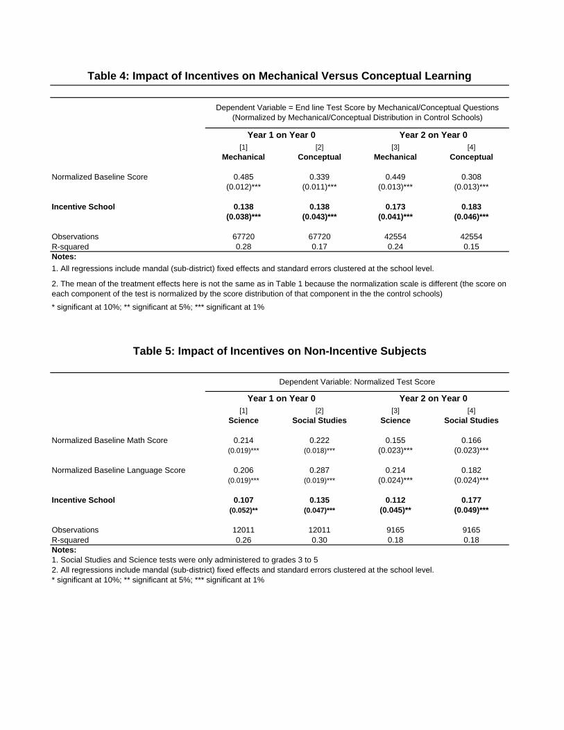
[1] [2] [3] [4]

Mechanical Conceptual Mechanical Conceptual

Normalized Baseline Score 0.485 0.339 0.449 0.308(0.012)*** (0.011)*** (0.013)*** (0.013)***

Incentive School 0.138 0.138 0.173 0.183(0.038)*** (0.043)*** (0.041)*** (0.046)***

Observations 67720 67720 42554 42554R-squared 0.28 0.17 0.24 0.15Notes:

* significant at 10%; ** significant at 5%; *** significant at 1%

[1] [2] [3] [4]

Science Social Studies Science Social Studies

Normalized Baseline Math Score 0.214 0.222 0.155 0.166(0.019)*** (0.018)*** (0.023)*** (0.023)***

Normalized Baseline Language Score 0.206 0.287 0.214 0.182(0.019)*** (0.019)*** (0.024)*** (0.024)***

Incentive School 0.107 0.135 0.112 0.177(0.052)** (0.047)*** (0.045)** (0.049)***

Observations 12011 12011 9165 9165R-squared 0.26 0.30 0.18 0.18Notes:1. Social Studies and Science tests were only administered to grades 3 to 52. All regressions include mandal (sub-district) fixed effects and standard errors clustered at the school level.* significant at 10%; ** significant at 5%; *** significant at 1%

Dependent Variable: Normalized Test Score

Year 1 on Year 0 Year 2 on Year 0

Table 4: Impact of Incentives on Mechanical Versus Conceptual Learning

Dependent Variable = End line Test Score by Mechanical/Conceptual Questions (Normalized by Mechanical/Conceptual Distribution in Control Schools)

Year 1 on Year 0 Year 2 on Year 0

Table 5: Impact of Incentives on Non-Incentive Subjects

2. The mean of the treatment effects here is not the same as in Table 1 because the normalization scale is different (the score on each component of the test is normalized by the score distribution of that component in the the control schools)

1. All regressions include mandal (sub-district) fixed effects and standard errors clustered at the school level.

[1] [2] [3] [4] [5] [6] [7] [8] [9]

Combined Maths Telugu Combined Maths Telugu Combined Maths Telugu0.499 0.490 0.516 0.559 0.505 0.618 0.451 0.417 0.485

(0.013)*** (0.017)*** (0.014)*** (0.018)*** (0.025)*** (0.014)*** (0.015)*** (0.022)*** (0.014)***

0.160 0.194 0.128 0.194 0.239 0.152 0.271 0.321 0.223(0.049)*** (0.060)*** (0.043)*** (0.049)*** (0.058)*** (0.044)*** (0.058)*** (0.068)*** (0.053)***

0.146 0.183 0.110 0.084 0.128 0.042 0.161 0.231 0.091(0.050)*** (0.058)*** (0.046)** (0.049)* (0.061)** (0.043) (0.058)*** (0.071)*** (0.052)*

0.790 0.870 0.683 0.045 0.096 0.026 0.116 0.291 0.03068678 34109 34569 63004 31443 31561 49498 24584 249140.29 0.28 0.32 0.30 0.28 0.34 0.23 0.23 0.25

Notes:All regressions include mandal (sub-district) fixed effects and standard errors clustered at the school level.* significant at 10%; ** significant at 5%; *** significant at 1%

Grade 2 Grade 3 Grade 4 Grade 5 Mechanical Conceptual Science Social Studies

[1] [2] [3] [4] [5] [6] [7] [8]

Individual Incentive 0.209 0.228 0.203 0.410 0.224 0.233 0.186 0.22(0.087)** (0.065)*** (0.086)** (0.081)*** (0.050)*** (0.057)*** (0.057)*** (0.060)***

Group Incentive 0.069 0.114 0.155 0.276 0.121 0.132 0.037 0.134(0.060) (0.080) (0.070)** (0.093)*** (0.051)** (0.057)** (0.056) (0.061)**

F-Stat p-value (Testing GI = II) 0.153 0.223 0.631 0.250 0.082 0.138 0.032 0.220Observations 49498 49498 49498 49498 42554 42554 9165 9165R-squared 0.23 0.23 0.23 0.23 0.24 0.16 0.19 0.18

Notes:1. Panels A and B combine normalized scores in both math and language2. All effects represent two year treatment effects (Y2 on Y0)3. All regressions include mandal (sub-district) fixed effects and standard errors clustered at the school level.* significant at 10%; ** significant at 5%; *** significant at 1%

Year 1 on Year 0 Year 2 on Year 1 Year 2 on Year 0

Table 6: Group versus Individual Incentives

Dependent Variable = Normalized Endline Test Score

Dependent Variable = Normalized Endline Test Score

Panel A: Impact of Incentive Type By GradePanel B: Impact of Incentive

Type on Mechanical vs Conceptual Learning

Panel C : Impact of Incentive Type on Non-Incentive

Subjects

Table 7: Disaggregated Treatment Effects By Individual And Group Incentives (Year 2 on Year 0)

R-squared

Normalized Lagged Score

Individual Incentive School (II)

Group Incentive School (GI)

F-Stat p-value (Testing GI = II)Observations

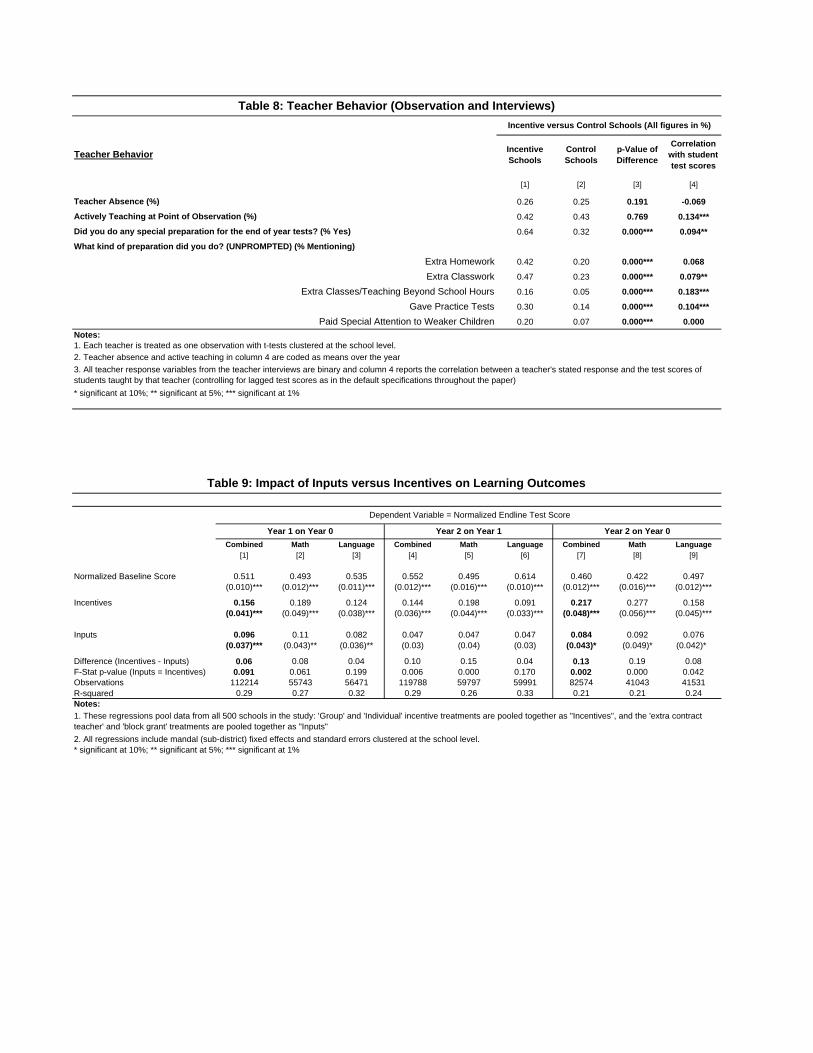
Incentive Schools

Control Schools

p-Value of Difference

Correlation with student test scores

[1] [2] [3] [4]

0.26 0.25 0.191 -0.069

0.42 0.43 0.769 0.134***

0.64 0.32 0.000*** 0.094**

0.42 0.20 0.000*** 0.068

0.47 0.23 0.000*** 0.079**

0.16 0.05 0.000*** 0.183***

0.30 0.14 0.000*** 0.104***

0.20 0.07 0.000*** 0.000

2. Teacher absence and active teaching in column 4 are coded as means over the year

Combined Math Language Combined Math Language Combined Math Language

[1] [2] [3] [4] [5] [6] [7] [8] [9]

Normalized Baseline Score 0.511 0.493 0.535 0.552 0.495 0.614 0.460 0.422 0.497(0.010)*** (0.012)*** (0.011)*** (0.012)*** (0.016)*** (0.010)*** (0.012)*** (0.016)*** (0.012)***

Incentives 0.156 0.189 0.124 0.144 0.198 0.091 0.217 0.277 0.158(0.041)*** (0.049)*** (0.038)*** (0.036)*** (0.044)*** (0.033)*** (0.048)*** (0.056)*** (0.045)***

Inputs 0.096 0.11 0.082 0.047 0.047 0.047 0.084 0.092 0.076(0.037)*** (0.043)** (0.036)** (0.03) (0.04) (0.03) (0.043)* (0.049)* (0.042)*

Difference (Incentives - Inputs) 0.06 0.08 0.04 0.10 0.15 0.04 0.13 0.19 0.08F-Stat p-value (Inputs = Incentives) 0.091 0.061 0.199 0.006 0.000 0.170 0.002 0.000 0.042Observations 112214 55743 56471 119788 59797 59991 82574 41043 41531R-squared 0.29 0.27 0.32 0.29 0.26 0.33 0.21 0.21 0.24Notes:

2. All regressions include mandal (sub-district) fixed effects and standard errors clustered at the school level.* significant at 10%; ** significant at 5%; *** significant at 1%

1. These regressions pool data from all 500 schools in the study: 'Group' and 'Individual' incentive treatments are pooled together as "Incentives", and the 'extra contract teacher' and 'block grant' treatments are pooled together as "Inputs"

Table 9: Impact of Inputs versus Incentives on Learning Outcomes

Dependent Variable = Normalized Endline Test Score

Year 1 on Year 0 Year 2 on Year 1 Year 2 on Year 0

* significant at 10%; ** significant at 5%; *** significant at 1%

Notes: 1. Each teacher is treated as one observation with t-tests clustered at the school level.

Paid Special Attention to Weaker Children

Extra Homework

3. All teacher response variables from the teacher interviews are binary and column 4 reports the correlation between a teacher's stated response and the test scores of students taught by that teacher (controlling for lagged test scores as in the default specifications throughout the paper)

Teacher Absence (%)

Gave Practice Tests

Extra Classes/Teaching Beyond School Hours

Table 8: Teacher Behavior (Observation and Interviews)

What kind of preparation did you do? (UNPROMPTED) (% Mentioning)

Did you do any special preparation for the end of year tests? (% Yes)

Extra Classwork

Actively Teaching at Point of Observation (%)

Teacher Behavior

Incentive versus Control Schools (All figures in %)

Figure 1a: Andhra Pradesh (AP)

Figure 1b: District Sampling (Stratified by Socio-cultural Region of AP)

6263Infant Mortality (per 1000)

25.325.2Teacher Absence (%)

60.564.8Literacy (%)

95.395.9Gross Enrollment (Ages 6-11) (%)

APIndia

6263Infant Mortality (per 1000)

25.325.2Teacher Absence (%)

60.564.8Literacy (%)

95.395.9Gross Enrollment (Ages 6-11) (%)

APIndia

Figure 2: Density/CDF of Normalized Test Scores by Treatment

Figure 3: Quantile (Percentile) Treatment Effects

0.1

.2.3

.4D

ensi

ty

-2 0 2 4 6Baseline Normalized Test Score

Control SchoolsIncentive Schools

0.2

.4.6

.81

Cum

ulat

ive

Dis

tribu

tion

-2 0 2 4 6Baseline Normalized Test Score

Control SchoolsIncentive Schools

0.1

.2.3

.4D

ensi

ty

-2 0 2 4 6Year 2 Normalized Test Score

Control SchoolsIncentive Schools

0.2

.4.6

.81

Cum

ulat

ive

Dis

tribu

tion

-2 0 2 4 6Year 2 Normalized Test Score

Control SchoolsIncentive Schools

-2-1

01

23

Yea

r 2 N

orm

aliz

ed T

est S

core

0 .2 .4 .6 .8 1Percentile of Endline Score

Control Schools Treatment Schools95% Confidence Interval Difference

Figure 4: Heterogeneous Treatment Effects by Baseline Score Percentile

Figure 5: Teacher Fixed Effects by Treatment Status

-.50

.51

Yea

r 2 N

orm

aliz

ed T

est S

core

0 .2 .4 .6 .8 1Percentile of Baseline Score

Control Schools Treatment Schools95% Confidence Interval Difference

-10

12

Teac

her F

ixed

Effe

ct in

SD

of s

tude

nt te

st s

core

s

0 .2 .4 .6 .8 1Percentile of Teacher Fixed Effect

Control Teachers Treatment Teachers95% Confidence Interval Difference