TCIAIG 1

Benchmarks for Grid-Based PathfindingNathan R. Sturtevant

Abstract—The study of algorithms on grids has beenwidespread in a number of research areas. Grids are easyto implement and offer fast memory access. Because of theirsimplicity, they are used even in commercial video games. But,the evaluation of work on grids has been inconsistent betweendifferent papers. Many research papers use different problemsets, making it difficult to compare results between papers.Furthermore, the performance characteristics of each test setare not necessarily obvious. This has motivated the creation of astandard test set of maps and problems on the maps that are openfor all researchers to use. In addition to creating these sets, weuse a variety of metrics to analyze the properties of the test sets.The goal is that these test sets will be useful to many researchers,making experimental results more comparable across papers, andimproving the quality of research on grid-based domains.

Index Terms—path planning, pathfinding, grid, search, map

I. INTRODUCTION

Grid-based maps have been widely used as test domainsin a number of fields, but until recently there was no pub-licly available standardized repository of problems for re-searchers. As a result we have created a pathfinding reposi-tory (http://www.movingai.com/benchmarks/) for storing bothmaps and problem sets that can be run on the maps.

This paper describes the data sets currently available online.We do not set out to describe a particular scientific advance-ment here. Instead, the goal is to describe the repository nowavailable, with the intent that the distribution of these mapsand problem sets will improve the quality and comparison ofwork that uses grids as test domains.

We encourage researchers to test algorithms on as manymaps as possible from the test sets, as this will help show thegenerality or the limitations of a given approach. Additionally,if researchers are working on techniques for video games, theywill find several sets of maps taken from commercial games.

In short, our goal is that this will improve the quality ofevaluation in our own and others’ scientific work.

We also describe a number of metrics which help typify thecharacteristics of each map. These help distinguish the featuresof each map type which might influence performance or theapplicability of a given approach.

When working on these test sets, we initially formed anumber of hypothesis about the properties of these maps. Westate them here with some justification, and then analyze howstrongly these predictions hold in practice.

• Scaling maps does not preserve all of the underlyingproperties of a map. Scaling a map will create larger openspaces and larger openings between distinct areas in theoriginal map. This isn’t to say that it is ‘wrong’ to scalea map, but that this change should be understood.

N. Sturtevant is with the Department of Computer Science, University ofDenver, Denver CO, 80208 USA e-mail: sturtevant@cs.du.edu.

• Artificial maps created algorithmically have differentproperties than maps created by designers for particularapplications. If an algorithm is being designed for aparticular application, it is important that the maps beingtested are similar to the application under consideration.

• There is a significant difference in the properties of agame map, depending on what genre of game the mapwas designed for. In role-playing games, players tend tohave a linear experience through a map, while real-timestrategy games are more about the strategic use of space,leading to less linear maps.

The rest of the paper is as follows. We begin by describingthe map format, as well as the types of maps available in therepository, and the source of these maps. Then we describehow the problem sets were built and the metrics that weuse for measuring the properties of the maps. Finally, weshow a number of experimental results across the domainsand provide a rough classification of the maps. We concludewith suggestions on use of these metrics.

II. MAP TYPES

Each of the following maps is available from an onlinepathfinding repository at http://movingai.com/benchmarks/.They are also available for anonymous SVN checkout froma google code repository:svn checkout http://hog2.googlecode.com/svn

/trunk/maps/ hog2-maps

All maps online are stored in the following format; some mapsin the repository use a more complex representation.

A. Map File Format Description

The map file format used in the repository was originallydeveloped by Yngvi Bjornsson and Markus Enzenberger at theUniversity of Alberta. We adapted this format as we beganimporting different types of maps from commercial games,but only the simplest format is described here.

The map format begins with the type, which is always‘octile’, followed by the dimensions of the map and thenthe map data itself. All cells in a map are either blocked orunblocked. However, to represent the underlying maps in amore artistic manner, several types of terrain have been added.Normal ground is represented by a period (‘.’), and shallowwater is represented by the ‘S’ character. These are the onlypassable types of terrain. All other terrain is considered tobe impassable, including trees (‘T’), water (‘W’) and out ofbounds (‘@’). This is illustrated in Figure 1. Part (a) of thefigure shows the textual representation of the map, while part(b) shows the graphical representation. Overlaid on the map isthe graph which represents the movement that can be taken onthe map. In this case, an agent in the map can walk between

TCIAIG 2

type octileheight 5width 10map@@@@@@@@@@TTWW@....@TTWW@....@TTSS@....@TTSS.....@

(a) (b)Fig. 1. Sample map text (a) and graphical (b) representation. The lines showthe connectivity between grid cells.

(a) (b)Fig. 2. Sample map from Baldur’s Gate II (a) and Dragon Age: Origins (b).

open ground and shallow water, but cannot traverse any otherterrain.

As shown in Figure 1, we assume that diagonal moves areonly possible if the related cardinal moves are both possible.That is, it is not possible to take a diagonal move between twoobstacles, and it is not possible to take a diagonal move to cuta corner. We make this assumption because in a real gameall creatures occupy some volume of space and are not ableto pass through blocked corners. The movement in the gameDragon Age: Origins, for instance, works with this assumption.

Following are the maps stored in the repository.

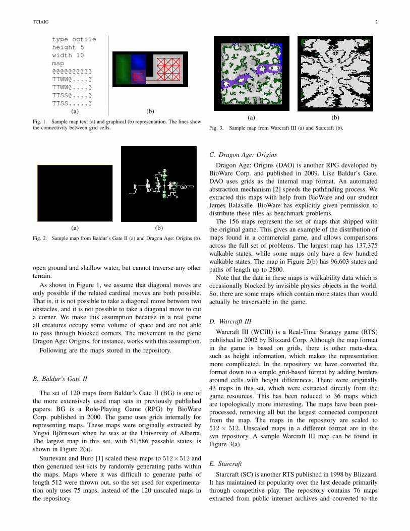
B. Baldur’s Gate II

The set of 120 maps from Baldur’s Gate II (BG) is one ofthe more extensively used map sets in previously publishedpapers. BG is a Role-Playing Game (RPG) by BioWareCorp. published in 2000. The game uses grids internally forrepresenting maps. These maps were originally extracted byYngvi Bjornsson when he was at the University of Alberta.The largest map in this set, with 51,586 passable states, isshown in Figure 2(a).

Sturtevant and Buro [1] scaled these maps to 512×512 andthen generated test sets by randomly generating paths withinthe maps. Maps where it was difficult to generate paths oflength 512 were thrown out, so the set used for experimenta-tion only uses 75 maps, instead of the 120 unscaled maps inthe repository.

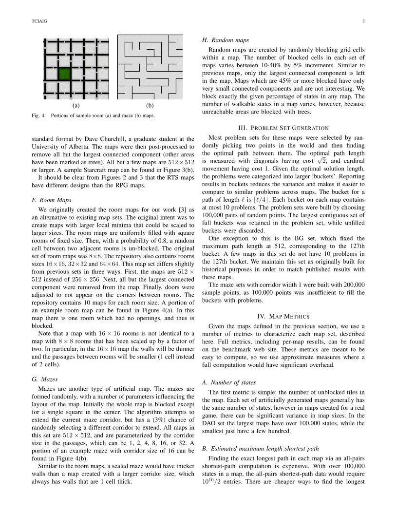
(a) (b)Fig. 3. Sample map from Warcraft III (a) and Starcraft (b).

C. Dragon Age: Origins

Dragon Age: Origins (DAO) is another RPG developed byBioWare Corp. and published in 2009. Like Baldur’s Gate,DAO uses grids as the internal map format. An automatedabstraction mechanism [2] speeds the pathfinding process. Weextracted this maps with help from BioWare and our studentJames Balasalle. BioWare has explicitly given permission todistribute these files as benchmark problems.

The 156 maps represent the set of maps that shipped withthe original game. This gives an example of the distribution ofmaps found in a commercial game, and allows comparisonsacross the full set of problems. The largest map has 137,375walkable states, while some maps only have a few hundredwalkable states. The map in Figure 2(b) has 96,603 states andpaths of length up to 2800.

Note that the data in these maps is walkability data which isoccasionally blocked by invisible physics objects in the world.So, there are some maps which contain more states than wouldactually be traversable in the game.

D. Warcraft III

Warcraft III (WCIII) is a Real-Time Strategy game (RTS)published in 2002 by Blizzard Corp. Although the map formatin the game is based on grids, there is other meta-data,such as height information, which makes the representationmore complicated. In the repository we have converted theformat down to a simple grid-based format by adding bordersaround cells with height differences. There were originally43 maps in this set, which were extracted directly from thegame resources. This has been reduced to 36 maps whichare topologically more interesting. The maps have been post-processed, removing all but the largest connected componentfrom the map. The maps in the repository are scaled to512 × 512. Unscaled maps in a different format are in thesvn repository. A sample Warcraft III map can be found inFigure 3(a).

E. Starcraft

Starcraft (SC) is another RTS published in 1998 by Blizzard.It has maintained its popularity over the last decade primarilythrough competitive play. The repository contains 76 mapsextracted from public internet archives and converted to the

TCIAIG 3

(a) (b)Fig. 4. Portions of sample room (a) and maze (b) maps.

standard format by Dave Churchill, a graduate student at theUniversity of Alberta. The maps were then post-processed toremove all but the largest connected component (other areashave been marked as trees). All but a few maps are 512×512or larger. A sample Starcraft map can be found in Figure 3(b).

It should be clear from Figures 2 and 3 that the RTS mapshave different designs than the RPG maps.

F. Room MapsWe originally created the room maps for our work [3] as

an alternative to existing map sets. The original intent was tocreate maps with larger local minima that could be scaled tolarger sizes. The room maps are uniformly filled with squarerooms of fixed size. Then, with a probability of 0.8, a randomcell between two adjacent rooms is un-blocked. The originalset of room maps was 8×8. The repository also contains roomssizes 16×16, 32×32 and 64×64. This map set differs slightlyfrom previous sets in three ways. First, the maps are 512 ×512 instead of 256× 256. Next, all but the largest connectedcomponent were removed from the map. Finally, doors wereadjusted to not appear on the corners between rooms. Therepository contains 10 maps for each room size. A portion ofan example room map can be found in Figure 4(a). In thismap there is one room which had no openings, and thus isblocked.

Note that a map with 16 × 16 rooms is not identical to amap with 8× 8 rooms that has been scaled up by a factor oftwo. In particular, in the 16×16 map the walls will be thinnerand the passages between rooms will be smaller (1 cell insteadof 2 cells).

G. MazesMazes are another type of artificial map. The mazes are

formed randomly, with a number of parameters influencing thelayout of the map. Initially the whole map is blocked exceptfor a single square in the center. The algorithm attempts toextend the current maze corridor, but has a (3%) chance ofrandomly selecting a different corridor to extend. All maps inthis set are 512× 512, and are parameterized by the corridorsize in the passages, which can be 1, 2, 4, 8, 16, or 32. Aportion of an example maze with corridor size of 16 can befound in Figure 4(b).

Similar to the room maps, a scaled maze would have thickerwalls than a map created with a larger corridor size, whichalways has walls that are 1 cell thick.

H. Random maps

Random maps are created by randomly blocking grid cellswithin a map. The number of blocked cells in each set ofmaps varies between 10-40% by 5% increments. Similar toprevious maps, only the largest connected component is leftin the map. Maps which are 45% or more blocked have onlyvery small connected components and are not interesting. Weblock exactly the given percentage of states in any map. Thenumber of walkable states in a map varies, however, becauseunreachable areas are blocked with trees.

III. PROBLEM SET GENERATION

Most problem sets for these maps were selected by ran-domly picking two points in the world and then findingthe optimal path between them. The optimal path lengthis measured with diagonals having cost

√2, and cardinal

movement having cost 1. Given the optimal solution length,the problems were categorized into larger ‘buckets’. Reportingresults in buckets reduces the variance and makes it easier tocompare to similar problems across maps. The bucket for apath of length ` is b`/4c. Each bucket on each map containsat most 10 problems. The problem sets were built by choosing100,000 pairs of random points. The largest contiguous set offull buckets was retained in the problem set, while unfilledbuckets were discarded.

One exception to this is the BG set, which fixed themaximum path length at 512, corresponding to the 127thbucket. A few maps in this set do not have 10 problems inthe 127th bucket. We maintain this set as originally built forhistorical purposes in order to match published results withthese maps.

The maze sets with corridor width 1 were built with 200,000sample points, as 100,000 points was insufficient to fill thebuckets with problems.

IV. MAP METRICS

Given the maps defined in the previous section, we use anumber of metrics to characterize each map set, describedhere. Full metrics, including per-map results, can be foundon the benchmark web site. These metrics are meant to beeasy to compute, so we use approximate measures where afull computation would have significant overhead.

A. Number of states

The first metric is simple: the number of unblocked tiles inthe map. Each set of artificially generated maps generally hasthe same number of states, however in maps created for a realgame, there can be significant variance in map sizes. In theDAO set the largest maps have over 100,000 states, while thesmallest just have a few hundred.

B. Estimated maximum length shortest path

Finding the exact longest path in each map via an all-pairsshortest-path computation is expensive. With over 100,000states in a map, the all-pairs shortest-path data would require1010/2 entries. There are cheaper ways to find the longest

TCIAIG 4

path, but a reasonably accurate estimation is sufficient for ourpurposes.

For each map we choose a random point and then perform aDijkstra search until the last state is found. Then, we measurethe longest path from this state. We do this 5 times for eachmap and take the maximum. Results are then averaged overall maps in a set. Mazes have, by far, the longest paths. Wewill discuss other correlations later.

C. Transit Node Count

The notions of transit nodes [4] and highway dimension [5]are metrics that have been used to describe why recent plan-ning approaches for road networks have been so successful.Transit nodes in a graph are the nodes at some small radiuswhich are on all shortest paths to nodes at a larger radius.When the number of transit nodes in a road graph is sparse, theall-pairs shortest-path data can be stored just between transitnodes, greatly reducing the storage overhead.

This concept has been generalized into the concept ofhighway dimension. Abraham et. al. [5] show that low high-way dimension guarantees efficient pre-processing and shortestpath queries for a number of planning algorithms, includingcontraction hierarchies [6] and reach [7].

Highway dimension is difficult to compute directly, becauseit requires an expensive optimization. Instead, we measure thenumber of transit nodes at radius r given shortest paths to 4r,for several values of r. This is a lower bound on the highwaydimension, and is measuring the same property – whether asparse set of points can be found on all shortest paths.

We randomly sampled 50 points on each map, measuringthe number of transit nodes for each point, and then averagethe results over all maps in each set. We report results forr = 10 and r = 40. If a map was completely explored beforereaching depth 4r the results were excluded from the reportedaverages.

A low highway dimension and/or transit node count sug-gests that memory-efficient heuristics can be built to solvepathfinding problems quickly.

D. Dimension

In addition to transit node count, we attempt to directlyestimate the dimension of a map. This is related to how thebranching factor might be estimated in an exponential tree.We do this by choosing a random point in a map and thenperforming a Dijkstra search, recording the number of nodesexpanded at each depth. Then we fit the number of states ateach depth to the polynomial a + b · x + c · x2 using linearregression. (The whole process is also called quadratic orpolynomial regression.) The value for c gives some indicationof the dimension of the map. If c = 0, the map is onedimensional. If c = 1 the map is two dimensional. If c < 0,the number of states at each new depth is being reduced. Thenumber of nodes expanded at the end of the search does tendto tail off as the ends of the map are reached, so we onlyperform the regression on the node counts from the first halfof the search. We repeated this measurement 50 times on eachmap. Results are then averaged over all maps.

Originally, our dimension metric was intended to estimatethe dimensions of a Euclidean heuristic [8], but experimentsshowed that results from these two approaches did not corre-late.

E. Heuristic Quality and Nodes Expanded

We use the problem sets to measure the quality of the searchheuristic in two ways. For all problems in bucket 127, whichhave length 508-512, we compare the initial heuristic value tothe optimal path cost and report the percentage. Many smallmaps do not have paths of this length, so this is biased towardslarger maps. We also measured the number of nodes expandedby A* when solving these problems and report this as well.

V. EXPERIMENTAL RESULTS

The average metrics for each problem set are in Table I.The first column is the map set. Results for the BG and WCIIImap sets are provided both for the original sizes and scaledto 512× 512. The artificial maps are all 512× 512, while theother maps are at their native resolutions.

The reported metrics are averages of the number of statesin the map, the maximum length shortest path, the dimen-sionality, the transit node count (TNC), and, for problemswith optimal length 508-512, the heuristic accuracy and nodesexpanded.

As the values reported are averages, there can be significantvariation, especially in the DAO set which contains a numberof small maps. We will look at this broad classification ofvalues; detailed results are available online.

The following data points are worth noting in the set; furtheranalysis follows in the next section.

• Increasing the size of the room maps increases thenumber of states in the map (because there are fewerwalls) and decreases the heuristic accuracy. The numberof nodes expanded in paths length 508-512 increasesslightly as the rooms get larger.

• Increasing the size of the maze corridors also increasesthe number of states in the map. It also increases theheuristic accuracy and the number of nodes expanded.Node expansions increase because larger corridors pro-vide more nodes for A* to expand. Heuristic accuracyincreases because the maximum path length decreases.

• As the random maps are progressively more filled, thenumber of states in the map decreases, but the nodes ex-panded increases. This is mirrored by a drop in heuristicaccuracy, meaning that the problems get harder as morerandom obstacles are added. But, when the map is 40%filled with obstacles, the problems begin to get easieragain.

• The transit node count is significantly higher at r = 10than at r = 40 on the room-64 and maze-32 maps.Recall that the transit node count is measured relative todistances r and 4r. At radius 40, most states will still beinside a room of size 64, increasing the TNC significantly.But, once the bulk of a search exits a door to a room, alloptimal paths will go through the same door, decreasing

TCIAIG 5

Average Average Tran. Node Cnt. Tran. Node Cnt. Heuristic ExpandedMap Set Num. States Max Path Dimension radius = 10 radius = 40 Accuracy (512) Nodes (512)BG 4,507 150.5 0.52 6.12 2.04 - -BG512 73,930 693.0 0.44 39.67 31.74 0.76 22,375.0DAO 21,323 427.4 0.31 11.05 3.32 0.59 17,857.6SC 263,782 1,190.2 0.41 40.11 15.44 0.78 26,993.3WCIII 10,669 155.5 0.70 6.26 2.06 - -WCIII512 90,910 674.0 0.75 32.27 13.30 0.84 27,386.4Rooms-8 206,792 891.7 0.78 5.32 9.15 0.86 40,414.8Rooms-16 231,263 863.8 0.94 3.94 6.54 0.83 41,776.3Rooms-32 243,733 881.0 0.97 4.16 4.77 0.83 45,210.7Rooms-64 249,352 931.0 0.81 30.04 3.20 0.77 50,467.7Mazes-1 131,071 7,575.6 0.01 1.82 1.82 0.18 4,619.0Mazes-2 174,517 5,795.1 0.02 1.86 1.73 0.24 8,671.6Mazes-4 209,268 4,849.1 0.03 1.90 1.81 0.27 14,972.9Mazes-8 232,928 4,526.0 0.03 2.14 1.85 0.34 19,768.0Mazes-16 246,042 3,826.5 0.02 5.81 1.93 0.41 27,693.8Mazes-32 253,819 2,666.4 0.03 22.89 2.77 0.49 39,123.8Random-10 235,903 766.8 1.13 16.93 22.79 0.99 14,696.4Random-15 222,689 789.9 1.01 14.34 19.97 0.97 21,728.9Random-20 209,255 816.6 0.92 11.70 16.80 0.95 28,408.8Random-25 195,315 851.1 0.79 9.33 13.68 0.91 33,447.2Random-30 180,209 894.4 0.64 6.81 10.81 0.86 34,956.9Random-35 161,313 983.5 0.50 4.26 6.86 0.76 35,540.7Random-40 96,365 1,585.1 0.09 2.42 2.36 0.46 19,555.8

TABLE IAVERAGE RESULTS FOR EACH MAP SET.

the TNC. A similar effect occurs in mazes with largercorridor sizes.

• The maze maps are the only set with dimension ofapproximately 0. As the search is constrained by the mazecorridors, no matter the size of the corridor, the numberof new states will tend to grow linearly with the depth.

Next we evaluate our three original hypothesis.

A. Evaluating Map Scaling

The first question we look at is the effect of scaling. Welook primarily at the BG maps, but the same trends hold forthe WCIII maps.

The unscaled maps have an average of 4,507 states, versus73,930 in the scaled maps. This is, of course, the motivation forinitially scaling these maps, as the originally maps were quitesmall and didn’t represent the work that might be requiredin a modern game. Our original hypothesis was that someproperties of maps are changed by scaling.

Results show that our measure of dimension is relativelyunchanged by scaling, while TNC is significantly changedby scaling. We plotted the dimension of the unscaled versusscaled maps, and then fit the resulting point cloud to a line.The points fit the line y = 0.01 + 0.98x with a correlationcoefficient of 0.96. This confirms that scaling a map leavesthe dimensionality unchanged. Our intuition behind this is thatthe relative size of areas stay the same when a map is scaled,so although more nodes will be expanded, the relative ratiosof nodes expanded at each depth stays the same.

Transit node count, however, changes significantly. Theunscaled BG maps have 6.12 transit nodes at radius 10 and2.04 transit nodes at radius 40. This is a significant departurefrom the result for the scaled maps, which have 39.67 transit

nodes at radius 10 and 31.74 transit nodes at radius 40. Givennormal tie-breaking rules (for expanding states with highest g-cost first) on an empty map all states at radius r will be on theshortest path to states at radius 4r. Scaling maps creates largeropen areas, and thus the number of transit nodes increases.Note, however, that this measurement depends on the radius.Given measurements at larger radii, we would expect thenumber of transit nodes to decrease.

These results suggest that scaling is not necessarily thewrong thing to do – it depends on how the maps are used.But the change in transit node count suggests that heuristicscould be less effective on scaled maps than unscaled ones.

B. Algorithmic Versus Designed Maps

Next we look at the maps which were generated algorith-mically in comparison to the other map sets. We performedanalysis of the metrics both manually and using k-meansclustering. All metrics were normalized (i.e. linearly mappedto [0, 1]), and then k-means clustering was run 1000 timeswith 4 and 7 clusters of maps. We kept track of how manytimes any pair of maps was placed in the same cluster witheach approach, and then looked at the top 20 pairings.

As expected, the artificial benchmark problems were verycommonly grouped together, as the metrics for these mapsare very similar. The exceptions to this was the Rooms-64 set,which is closest to the SC map set, and the Random-40 whichis closest to the DAO map set. With 40% random obstaclesthe optimal paths in a map no longer resemble a straight line,as they do with fewer obstacles. Instead the obstacles formareas more analogous to the rooms and corridors which areseen in the DAO maps. The BG512 and WCIII512 map setswere almost always grouped together and show reasonable

TCIAIG 6

similarity. This shows that in some cases algorithmicallydesigned maps share metrics with human-designed maps, butnot in the majority of cases.

C. Genre-Specific Differences

Finally, we look at the difference between maps for role-playing games (RPGs) and real-time strategy games (RTS).We focus on the DAO and SC sets which are not scaled. Wesee that the SC maps have more states and longer paths onaverage. They also have much higher TNC. This is partially aselection bias – the SC maps are being used in competitionsand are not the maps that would be used in a play-throughof a game. But, on the SC maps, a typical problem of length512 would require 10% of the map states to be expanded,while the DAO problems would require 50% of the mapstates to be expanded. This is computed by looking at theaverage number of states in maps with paths length 508-512.This suggests that the SC maps are more two-dimensional: Aheuristic search across a two-dimensional plane will expanda smaller fraction of the total states than a heuristic searchalong a one-dimensional line. But, this is contradicted by ourmeasure of dimension, which shows the SC maps with 0.41versus the DAO maps with 0.31. Further analysis revealed thedifference: the average dimension of maps that contain pathsof length 400 or longer is 0.07. Thus, larger DAO maps havelower dimension. This reveals that, for larger maps, there is aclear structural difference between SC and DAO maps.

VI. CONCLUSIONS

This paper describes a new repository that has been placedonline to improve the evaluation of grid-based problems. Thisrepository will allow researchers to use the same problems andtest sets, increasing the reproducibility of published results.We introduce the data sets, describe how they were built, andprovide metrics for distinguishing map types.

We provide the following suggestions for researchers usingthese problem sets:

• Report exactly which map set was used.• Report exactly what problems were used. For example, a

given bucket size across all maps in a particular problemset.

• Use the existing problem sets. This will allow otherresearchers to exactly duplicate your results.

• Report any deviation from the testing conditions. Thesecould include different edge costs (e.g., 1.5 for diago-nals for more efficient search), a different heuristic, orallowing agents to cut corners.

• Use a broad set of test maps to clearly illustrate thestrengths and weaknesses of a given approach. For in-stance, techniques that work particularly well on mapswith axis-aligned obstacles should not be exclusivelytested on artificial benchmarks. If you are unsure ofthe limitations of your approach, use the benchmarksto explore them, and test to see if any of the providedmetrics correlate with performance.

We have made some effort to collect an interesting set ofmaps and provide useful metrics to analyze them. But, we

are open to adding more map sets or metrics if they can bedemonstrated to provide useful classification. We are also opento adding other map formats to the repository.

Authors are encouraged to send us any papers publishedusing these benchmarks as we are maintaining a list of paperswhich use them. Currently over 30 published papers haveused these maps or benchmark problems starting in 2004 [9]and continuing to the present [10]. We hope that many moreresearchers will benefit from their broader public distribution.

ACKNOWLEDGEMENTS

We acknowledge the help of Chris Rayner in helping to measurethe correlation between our dimension metric and the dimensioncomputed by Euclidean heuristics.

REFERENCES

[1] N. R. Sturtevant and M. Buro, “Partial pathfinding using map abstractionand refinement,” in AAAI, 2005, pp. 1392–1397.

[2] N. R. Sturtevant, “Memory-efficient abstractions for pathfinding,” inAIIDE, 2007, pp. 31–36.

[3] N. R. Sturtevant, A. Felner, M. Barrer, J. Schaeffer, and N. Burch,“Memory-based heuristics for explicit state spaces,” in IJCAI, 2009, pp.609–614. [Online]. Available: http://ijcai.org/papers09/Papers/IJCAI07-107.pdf

[4] H. Bast, S. Funke, and D. Matijevic, “Transit ultrafast shortest-path queries with linear-time preprocessing,” in In 9th DIMACSImplementation Challenge, 2006.

[5] I. Abraham, A. Fiat, A. V. Goldberg, and R. F. Werneck, “Highwaydimension, shortest paths, and provably efficient algorithms,” inProceedings of the Twenty-First Annual ACM-SIAM Symposium onDiscrete Algorithms, ser. SODA ’10. Philadelphia, PA, USA: Societyfor Industrial and Applied Mathematics, 2010, pp. 782–793. [Online].Available: http://portal.acm.org/citation.cfm?id=1873601.1873665

[6] R. Geisberger, P. Sanders, D. Schultes, and D. Delling, “Contractionhierarchies: Faster and simpler hierarchical routing in road networks,”in WEA, 2008, pp. 319–333.

[7] A. V. Goldberg, H. Kaplan, and R. F. Werneck, “Reach for a*: Effi-cient point-to-point shortest path algorithms,” in IN WORKSHOP ONALGORITHM ENGINEERING AND EXPERIMENTS, 2006, pp. 129–143.

[8] D. C. Rayner, M. H. Bowling, and N. R. Sturtevant, “Euclideanheuristic optimization,” in AAAI, 2011. [Online]. Available:http://www.aaai.org/ocs/index.php/AAAI/AAAI11/paper/view/3594

[9] A. Botea, M. Muller, and J. Schaeffer, “Near Optimal Hierarchical Path-Finding,” Journal of Game Development, vol. 1, no. 1, pp. 7–28, 2004.

[10] C. Hernandez and J. A. Baier, “Fast subgoaling for pathfinding via real-time search,” in ICAPS, 2011.

Nathan Sturtevant is Assistant Professor in theComputer Science Department at the University ofDenver. His scientific research focuses on Artifi-cial Intelligence and search in single and multi-agent settings, including applications to real-timeenvironments, such as games, and more competitiveenvironments.