Taylor Polynomials with Error Term

The functionsex, sinx, 1/√

1−x, etc are nice functions but they are not as nice as polynomials.Specifically polynomials can be evaluated completely based on multiplication, subtraction andaddition (realizing that integer powers are just multiple multiplications). Thus when you buildyour computer, if you teach it how to multiply, subtract and add, your computer can also evaluatepolynomials. These other functions are not that simple (even division creates many problems). Theway that computers evaluate the more complex functions is to approximate them by polynomials.

There are many other applications where it is useful to have a polynomial approximation toa function. Generally, polynomials are just easier to use. In this section we will show you howto obtain a polynomial approximation of a function. The approximation will include the errorterm—extremely important since we must know that our approximation is a sufficiently goodapproximation—how good depends on our application. The main tool that we will use is inte-gration by parts. Specifically, we will use integration by parts in the formZ b

aF ′Gdt = [FG]ba−

Z b

aFG′dt.

If you are not particularly familiar with this form of integration by parts, you should review exactlywhy this form is the same as the

Rudv, etc, form of integration by parts.

We consider the functionf and desire to find a polynomial approximation off nearx = 0. We

begin by noting thatZ x

0f ′(t)dt = f (x)− f (0) or

f (x) = f (0)+Z x

0f ′(t)dt (1)

If we write expression (1) asf (x) = T0(x)+R0(x) whereT0(x) = f (0) andR0(x) =R x

0 f ′(t)dt,thenT0 would be referred to as the zero orderTaylor polynomial of the function f aboutx = 0andR0 would be the zero ordererror term —of course the trivial case—and generallyT0 wouldnot be a very good approximation off .

We obtain the next order of approximation by integratingR x

0 f ′(t)dt by parts. We letG = f ′,F ′ = 1. ThenG′ = f ′′ andF = t−x. You should note the last step carefully. The dummy variablein the integral

R x0 f ′(t)dt is t. Hence, if you were to integrate by parts with out being especially

clever (or even sneaky), you would say thatF = t. However, there is no special reason that youcould not useF = t + 1 or F = t + π instead. The only requirement is that the derivative ofFmust be 1. Since the integration (and hence, the differentiation) is with respect tot, x is a constantwith respect to this operation (no different from 1 orπ) andwe want it, it is perfectly OK to setF = t−x. Then application of integration by parts gives

Z x

0f ′(t)dt =

Z x

0F ′Gdt = [FG]x0−

Z x

0FG′dt

=Z x

01· f ′(t)dt =

[(t−x) f ′(t)

]t=xt=0−

Z t=x

t=0(t−x) f ′′(t)dt

= 0− (−x) f ′(0)−Z x

0(t−x) f ′′(t)dt = x f ′(0)−

Z x

0(t−x) f ′′(t)dt.

1

If we plug this result into (1), we get

f (x) = f (0)+x f ′(0)−Z x

0(t−x) f ′′(t)dt (2)

Expression (2) can be written asf (x) = T1(x)+R1(x) whereT1(x) = f (0)+x f ′(0) is the first

orderTaylor polynomial of f at x = 0 andR1(x) = −Z x

0(t − x) f ′′(t)dt is the first ordererror

term. At this time it is not clear thatT1 is a better approximation off thanT0. We must be patient.

Note: In the computation above we used the notationt = x and t = 0 on the integral and theevaluation bracket. This was done to try to emphasize the fact that the variable being substitutedand the dummy variable in the integral ist.

We continue by again integrating the integral in expression (2) by parts. We letG = f ′′, F =(t−x), getG′ = f ′′′ andF = 1

2(t−x)2, and eventually get

f (x) = f (0)+x f ′(0)+12

x2 f ′′(0)+12

Z x

0(t−x)2 f ′′′(t)dt (3)

And it should not be surprising that we write this asf (x) = T2(x)+R2(x) whereT2 andR2 arethe second orderTaylor polynomial of f atx = 0 anderror term , respectively.

By now it is possible to start seeing how and whyT2 approximatesf . The approximation isgoing to be a good approximation (in this case because 2 is still a small number, a relatively goodapproximation) for values ofx near zero, i.e. for small values ofx. If x is small andt is between0 andx, t − x will be small. And,(t − x)2 will be smaller yet. Thus iff ′′′ is small—or at leastbounded, then for small values ofx, R2(x) will be small andf (x)∼= T2(x) where the approximationis only as good asR2(x) is small.

Homework 1: Verify expression (3).

Homework 2: By integrating the integral in (3) by parts, derive the expressionf (x) = T3(x)+R3(x) with the appropriate definitions ofT3 andR3.

After you do HW2 we say etc. (or if we want to be more rigorous, we use mathematical

induction) and obtain (remember thatj! = 1·2· · · · · j and thatf (n) = f′′···′︸︷︷︸

n ):

f (x) =n

∑j=0

1j!

x j f ( j)(0)+(−1)n 1n!

Z x

0(t−x)n f (n+1)(t)dt = Tn(x)+Rn(x) (4)

whereTn is then-th orderTaylor polynomial of f at x = 0 andRn is then-th ordererror term ,i.e.

Tn(x) =n

∑j=0

1j!

x j f ( j)(0) (5)

2

Rn(x) = (−1)n 1n!

Z x

0(t−x)n f (n+1)(t)dt (6)

You might have noticed that every time we said that something was the Taylor polynomial, weadded the expression “off at x = 0” or “of f aboutx = 0”. The reason that we keep telling youthat it is the Taylor polynomial atx = 0 is because we are expanding the function aboutx = 0 (thatis why it depends off and the derivatives off evaluated atx = 0). In the next section we willexpand functions about points other than zero.

We now consider the following example.

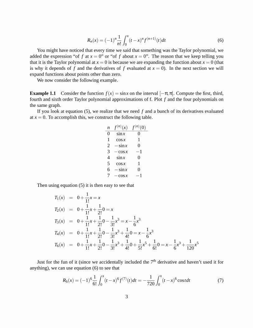
Example 1.1 Consider the functionf (x) = sinx on the interval[−π,π]. Compute the first, third,fourth and sixth order Taylor polynomial approximations of f. Plotf and the four polynomials onthe same graph.

If you look at equation (5), we realize that we needf and a bunch of its derivatives evaluatedatx = 0. To accomplish this, we construct the following table.

n f (n)(x) f (n)(0)0 sinx 01 cosx 12 −sinx 03 −cosx −14 sinx 05 cosx 16 −sinx 07 −cosx −1

Then using equation (5) it is then easy to see that

T1(x) = 0+11!

x = x

T2(x) = 0+11!

x+12!

0 = x

T3(x) = 0+11!

x+12!

0− 13!

x3 = x− 16

x3

T4(x) = 0+11!

x+12!

0− 13!

x3 +14!

0 = x− 16

x3

T6(x) = 0+11!

x+12!

0− 13!

x3 +14!

0+15!

x5 +16!

0 = x− 16

x3 +1

120x5

Just for the fun of it (since we accidentally included the 7th derivative and haven’t used it foranything), we can use equation (6) to see that

R6(x) = (−1)6 16!

Z x

0(t−x)6 f (7)(t)dt =− 1

720

Z x

0(t−x)6costdt (7)

3

Note 1: We notice that even coefficients (coefficients of even powers ofx) are all zero. Only oddpowers ofx are included in the expansion. We want to emphasize that this is not always the case.This happens in this case because the sine function is an odd function so the Taylor polynomialapproximating the sine function will also be an odd function—and the way that a Taylor polynomialis an odd function is by containing only odd powers ofx. The reason that this happens is whenevera function is an odd function about zero, then all of the even derivatives evaluated at zero will bezero. Can you prove that?

Note 2: (Hint: This note is not easy—but it may be useful.) If we consider the expression forR6

given in (7), we see that forx≥ 0

|R6(x)| =∣∣∣∣ 1720

Z x

0(t−x)6costdt

∣∣∣∣≤ 1720

Z x

0

∣∣∣(t−x)6∣∣∣ |cost|dt

≤ 1720

Z x

0

∣∣∣(t−x)6∣∣∣dt because|cost| ≤ 1

=1

720·7|x|7

The first inequality is due to a common property of integrals that apparently is not included in

our text: If f is integrable, then

∣∣∣∣Z b

af (t)dt

∣∣∣∣ ≤ Z b

a| f (t)|dt. If we assume that bothf and| f | are

integrable, then the property follows from Property 7, page 347 (since−| f (t)| ≤ f (t) ≤ | f (t)|).The last equality is true if you just consider the integral carefully, using the fact thatx≥ 0 impliesthatx≥ t. Of course the absolute value sign in the last expression is not needed—we want it therebecause the end result is true whenx is either positive or negative. Whenx≤ 0, we see that

|R6(x)| =∣∣∣∣ 1720

Z x

0(t−x)6costdt

∣∣∣∣ =∣∣∣∣ 1720

Z 0

x(t−x)6costdt

∣∣∣∣≤ 1720

Z 0

x

∣∣∣(t−x)6∣∣∣ |cost|dt

≤ 1720

Z 0

x

∣∣∣(t−x)6∣∣∣dt =

1720·7

|x|7 .

(Remember that whenx≤ 0, |x|=−x.)Hence in either case we have|R6(x)| ≤ 1

720·7 |x|7. If we want to considerx ∈ [−.5, .5], then

|R6(x)| ≤ 1720·7 |.5|

7 ≤ 1.550099206·10−6. Thus usingT6 as an approximation of the sine functionis a very good approximation if we limitx to be in the interval[−.5, .5].

One of the ways that makes it reasonably easy to see what is happening is to plot the Taylorpolynomials and the function. (You should understand that the plot given below is very nice butit does not take the place of the analysis done above. The results of the plot are only as good asthe plotter.) On the plot given in Figure 1 you see that there are four functions plotted:y = sinx,y = T1(x) (which is identical toy = T2(x)) y = T3(x) (= T4(x)) andy = T6(x).

It looks as ifT1 is a pretty good approximation toy= sinx nearx= 0 (which shouldn’t surpriseus sincey = T1(x) represents the tangent to the curvey = sinx at x = 0. It should be pretty clearthaty = T3(x) is a better approximation toy = sinx thaty = T1(x) and thaty = T6(x) is better than

4

y = T3(x). If you look carefully (and have a good eye), it appears thatT6 is a good approximationwell beyond the[−.5, .5] interval analyzed above. You must remember that there are inequalitiesinvolved in the analysis above—that means that the results might be better than we computed themto be.

Figure 1: Taylor polynomial approximations fory = sinx

Example 1.2Consider the functionf (x) = e3x on the interval[−2,2]. Compute the third,fourth, sixth and eighth order Taylor polynomial approximations off . Plot f and the four polyno-mials on the same graph.

5

We begin by constructing the following table.

n f (n)(x) f (n)(0)0 e3x 11 3e3x 32 9e3x 93 27e3x 274 81e3x 815 243e3x 2436 729e3x 7297 2187e3x 21878 38e3x 38

9 39e3x 39

Using equation (5) we see that

T3(x) =10!

+31!

x+32

2!x2 +

33

3!x3 = 1+3x+

92

x2 +92

x3

=3

∑k=0

3k

k!xk

T4(x) =10!

+31!

x+32

2!x2 +

33

3!x3 +

34

4!x4 = 1+3x+

92

x2 +92

x3 +278

x4

=4

∑k=0

3k

k!xk

T6(x) =10!

+31!

x+32

2!x2 +

33

3!x3 +

34

4!x4 +

35

5!x5 +

36

6!x6

= 1+3x+92

x2 +92

x3 +278

x4 +8140

x5 +8180

x6

=6

∑k=0

3k

k!xk

T8(x) =10!

+31!

x+32

2!x2 +

33

3!x3 +

34

4!x4 +

35

5!x5 +

36

6!x6 +

37

7!x7 +

38

8!x8

= 1+3x+92

x2 +92

x3 +278

x4 +8140

x5 +8180

x6 +243560

x7 +7294480

x8

=8

∑k=0

3k

k!xk

We see that it is not much fun to calculate Taylor polynomials for very largen (at least I didn’tenjoy it). In the lab we shall see that these polynomials can be easily computed using Maple orMatlab—and for much largerns than 8. In Figure 2 we see that they all do well in approximatinge3x nearx = 0. We also note that they all do poorly for negativex less than 1.5. And hopefullyyou’d expect by now,T8 does better than the others in general.

6

Figure 2: Taylor polynomial approximations fory = e3x

Note 1: As a part of the calculation we see that even though 3k grows fast, eventually we see thatk! grows faster. This can be seen using the techniques of Section 7.6.

Note 2: We see that by equation (6)

R8(x) = (−1)8 18!

Z x

0(t−x)8 f (9)(t)dt =− 1

51840

Z x

0(t−x)839e3tdt (8)

If we now bound the error term as we did in Example 1.1, forx∈ [−2,2] we get

|R8(x)|=∣∣∣∣ 151840

Z x

0(t−x)839e3tdt

∣∣∣∣≤ 39e6

51840

Z x

0

∣∣(t−x)8∣∣dt =

39e6

51840|x|9

(9)

It should be noted that thee6 term is in the last expression because we bounded the functione3t

on [−2,2] by e6. If we apply inequality (9) on the entire interval[−2,2], set|x| = 2, we see that

7

|R8(x)| ≤ 8714.1 — which is not very good. If we looked at the plots given in Figure 2, we knewthat the approximation would not be good but we wouldn’t think it would be this bad. We mustremember that this is an inequality. If we look at the picture very carefully, the difference betweenT8 ande3t is about 17.2, and it is true that 17.2≤ 8714.1. Even on the interval[−1.5,1.5] whereby the plots in Figure 2 we see thatT8 is clearly a pretty good approximation ofe3t , we find that|R8(x)| ≤ 654.3 (and we could have done a little better if we have boundede3t by e4.5 on [−1.5,1.5]instead of —and gotten 146.0 instead). Again the emphasis is that the result we get from (9) is aninequality. If we setx = .5, we get|R8(x)| ≤ 0.033, which is not great but is reasonably nice.

Homework 3: Compute the fifth order Taylor polynomial of the function11−x atx = 0.

Homework 4: Compute the third order Taylor polynomial of the function 2−x+3x2−2x3+x4

atx = 0. ComputeR3 and show why you know why it is correct.

8

More Taylor Polynomials with Error Term

We emphasized in the last section (and we saw it in the plots) that our approximations were ap-proximations nearx = 0. In this section we develop the analogous results for approximations of afunction f nearx = a for an arbitrarya. We mimic what we did in the previous section but we start

with consideringZ x

af ′(t)dt = f (x)− f (a) or

f (x) = f (a)+Z x

af ′t(t)dt (10)

Of course this gives us the zeroth orderTaylor polynomial of f aboutx= a and the associatedzeroth ordererror term . We again integrate the integral in (10) by parts, settingG= f ′ andF ′ = 1.We getG′ = f ′′, F = t − x (again thet − x instead of just thet—wherex is just a constant withrespect to this integration), and

Z x

af ′(t)dt =

[(t−x) f ′(t)

]t=xt=a−

Z x

a(t−x) f ′′(t)dt

= 0− (a−x) f ′(a)−Z x

a(t−x) f ′′(t)dt = (x−a) f ′(a)−

Z x

a(t−x) f ′′(t)dt.

Thus we have

f (x) = f (a)+(x−a) f ′(a)−Z x

a(t−x) f ′′(t)dt = T1(x)+R1(x) (11)

whereT1(x) = f (a) + (x− a) f ′(a) is the first orderTaylor polynomial of f aboutx = a and

R1(x) =−Z x

a(t−x) f ′′(t)dt is the first order error term.

Hopefully by now it should be easy to compute

f (x) = f (a)+(x−a) f ′(a)+12(x−a)2 f ′′(a)+

12

Z x

a(t−x)2 f ′′′(t)dt = T2(x)+R2(x) (12)

the second orderTaylor polynomial of f aboutx = a and the second order error term, and ingeneral

f (x) =n

∑j=0

1j!

f ( j)(a)(x−a) j +(−1)n

n!

Z x

a(t−x)n f (n+1)(t)dt = Tn(x)+Rn(x) (13)

where

Tn(x) =n

∑j=0

1j!

f ( j)(a)(x−a) j (14)

is then-th orderTaylor polynomial aboutx = a and

Rn(x) =(−1)n

n!

Z x

a(t−x)n f (n+1)(t)dt (15)

is then-th ordererror term .

9

Homework 5: Verify expression (13). (Verify that the form of the Taylor polynomial given in(13) matches that given in (12). Verify by taking one more step of integration by parts that therewill be a j! in the denominator. Verify that(−1)n term inRn appears to be correct.)

We next see that computing Taylor polynomials aboutx = a is very much the same as comput-ing Taylor polynomials aboutx = 0.

Example 2.1 Compute the third and fourth order Taylor polynomials off (x) = 1x+1 aboutx = 2.

Plot f and the two polynomials on the same graph.Again we the construct the table of derivatives as follows.

n f (n)(x) f (n)(2)0 (x+1)−1 3−1

1 −(x+1)−2 −3−2

2 2!(x+1)−3 2! ·3−3

3 −3!(x+1)−4 −3! ·3−4

3 4!(x+1)−5 4! ·3−5

5 −5!(x+1)−6 −5! ·3−6

Applying equation (14) we see that

T3(x) =3

∑j=0

1j!

(x−a) j f ( j)(a)

=10!

(x−2)0 f (2)+11!

(x−2) f ′(2)+12!

(x−2)2 f ′′(2)+13!

(x−3)2 f ′′′(2)

=10!

(x−2)013

+11!

(x−2)(− 1

32

)+

12!

(x−2)2 2!33 +

13!

(x−3)2(−3!

34

)=

13− 1

9(x−2)+

127

(x−2)2− 181

(x−2)3 and

T4(x) = T3(x)+14!

(x−2)4 f (4)(2)

=13− 1

9(x−2)+

127

(x−2)2− 181

(x−2)3 +1

243(x−2)4

Below in Figure 3 we see that bothT3 andT4 approximatef well nearx= 2. Careful inspectionalso shows thatT4 approximatesf better thanT3.

If we treated this problem as we did Examples 1.1 and 1.2, we would next treat the error termto bound the errors terms associated withT3 andT4 and, hence, have an analytic bound on the errorof approximation. Instead we shall state and prove (sort of) the following theorem.

Theorem 1.1 (Taylor Inequality) Suppose the functionf and the firstn+1 derivatives off are

integrable. Suppose thatM is such that max

{∣∣∣ f (n+1)(x)∣∣∣ ∣∣∣∣ |x−a| ≤ d

}≤ M. Then

|Rn(x)| ≤M

(n+1)!|x−a|n+1

10

Figure 3: Taylor polynomial approximations fory = 1x+1

We treat this result just as we bounded the error terms in Examples 1.1 and 1.2. We see that

|Rn(x)| =∣∣∣∣(−1)n

n!

Z x

a(t−x)n f (n+1)(t)dt

∣∣∣∣≤ 1n!

∣∣∣∣Z x

a|(t−x)n|

∣∣∣ f (n+1)(t)∣∣∣dt

∣∣∣∣≤ M

n!

∣∣∣∣Z x

a|(t−x)n|dt

∣∣∣∣ =Mn!|x−a|n+1

n+1=

M(n+1)!

|x−a|n+1

Notice that in the right hand side of the first inequality we have taken the absolute value insideof the integral and outside of the integral. The absolute value that is outside of the integral isnecessary to cover the case whenx < a. Of course the second inequality is due to the assumedbound on the absolute value off . And finally, the final result is obtained by integrating(t−x)n. Tonot allow the absolute value inside of the integral to bother us, it is easiest to perform the integraltwice, once assuming thatx > a and once assuming thatx < a.

We can then return to the example considered in Example 2.1.

11

Example 2.2: Use the Taylor Inequality to bound the error due to the approximation off (x) =1

x+1 by T3 andT4 on the interval[1.5,2.5].To emphasize what we are doing we writeR3(x) = f (x)−T3(x), note thatf (4)(x) = 4!/(x+1)5

and∣∣∣ f (4)(x)

∣∣∣≤ 4!/2.55 (evaluate the function atx = 1.5) and apply Taylor’s Inequality to get

|R3(x)| ≤4!/2.55

4!|x−2|4 ≤ .54

2.55 = 0.00064

Thus we see that forx∈ [1.5,2.5], | f (x)−T3(x)| ≤ 0.00064 — not a bad approximation.Repeating this process forn = 4, we get

|R4(x)| ≤5!/2.56

5!|x−2|5 ≤ .55

2.56 = 0.000128

We should emphasize that in the case whenn = 3, we get the boundM = 4!/2.55 and whenn= 4, we getM = 5!/2.56. These bounds are obtained by evaluatingf (4)(x) and f (5)(x) atx= 1.5.The easiest was to see that the maximums off (4)(x) and f (5)(x) occur atx = 1.5 is to graph thefunctions on the interval[1.5,2.5]. It should be clear that the maximum values of the absolutevalues of these functions occur atx = 1.5.

Homework 6: Evaluate the fourth order Taylor approximation aboutx = −1 of the functionf (x) = e3x on the interval[−1.5,−0.5] and use the Taylor Inequality to determine a bound for theerror of the approximation.

Homework 7: Evaluate the fifth order Taylor approximation aboutx = π of the functionf (x) =cosθ on the interval[π/3,5π/3] and use the Taylor Inequality to determine a bound for the errorof the approximation. (Hint: It is sometime difficult to find the maximum of some functions onsome intervals. For something like the sine and cosine functions, using 1 is the maximum of theabsolute value isusually a good enough bound the function on any interval.)

12

Motivation of Series

In the last three sections we have seen that it is possible to approximate functions by polynomials.We have seen that the approximation might be quite good on some intervals and not so good onother intervals. We have seen the approximation is determined by the error term—and that errorterm is a pain to deal with. From what we have seen, we would have guess that ifT8 is a prettygood approximation off (x) = e3x, then how well mightT100 (we first wrote out the expression forT100 but then decided that we would not waste the space—you can see what it looks like in the lab)approximatee3x? We do know that the hundred and first derivative isf (101)(x) = 3101e3x, so on[−5,5]

|R101| ≤3101e15

101!5101−2.1150·10−35.

We’d have to agree that this result is very good. We clearly could do pretty well on a largerinterval. But obviouslyT100 is not equal to f . There are times when we want to replacef by the“polynomial”. We can’t do that withT100. There are times when it is not good enough to have anapproximation. The obvious approach is to use a larger order yet. If we liked

f (x)∼= T100(x) =100

∑k=0

3k

k!xk

how about∞

∑k=0

3k

k!xk (16)

Before we can consider how or if this might work or be useful, we must decide what it meansor if it can mean anything logical. Easier yet, we might consider whether (16) makes any sense fora fixed value ofx, sayx = 1, i.e. does it make any sense to write

∞

∑k=0

3k

k!1k = 1+3+

92

+278

+ · · · (17)

In the next sections we show you how to decide whether or not an expression such as (17)makes any sense. We will decide when infinite sums such as (17) converge (sum to some number)or do not converge. After we understand what we mean by convergence (sums) of expressions like(17), we return to infinite sums of functions such as is given in (16). Functions given in the formof (16) have been and are still very useful in many areas of mathematics.

13