Introduction The model Nash equilibrium Numerical illustration

Tax Me if you Can!Optimal Nonlinear Income Tax between Competing

Governments

Etienne LEHMANN1

Laurent SIMULA2

Alain TRANNOY3

PET 2014

1CRED – University Paris 2 and CREST2Uppsala University.3Aix–Marseille School of Economics.

1 / 28

Introduction The model Nash equilibrium Numerical illustration

Motivation

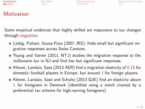
Some empirical evidences that highly skilled are responsive to tax changesthrough migration.

Liebig, Puhani, Sousa-Poza (2007 JRS): finds small but significant mi-gration responses across Swiss Cantons.

Young and Varner (2011, NTJ) studies the migration response to themillionaire tax in NJ and find low but significant responses.

Kleven, Landais, Saez (2013 AER) find a migration elasticity of 0.15 fordomestic football players in Europe, but around 1 for foreign players.

Kleven, Landais, Saez and Schultz (2013 QJE) find an elasticity above1 for foreigners in Denmark (identified using a notch created by apreferential tax scheme for high-earning foreigners).

2 / 28

Introduction The model Nash equilibrium Numerical illustration

Main question

How different is the nonlinear income tax schedule that a government findsoptimal when workers can vote with their feet?

How the optimal tax schedule is affected by tax competition?

What sufficient statics do we need to estimate?

3 / 28

Introduction The model Nash equilibrium Numerical illustration

Main features of the model

Two countries (not necessarily symmetric).

Individuals differ with respect to their skills and migration costs.

In each country, a government sets the nonlinear income tax, takinginto account intensive labor supply and migration responses.

Focus on the Nash equilibrium between two Maximin governments.

Identify key parameters to estimate: semi-elasticity of migration andhow it evolves along the skill distribution.

Definition (Migration responses at a given skill level)

Semi-elasticity: percentage change in the density of taxpayers of a given skilllevel when their consumption is increased by $1.

Elasticity:“... by 1%”= consumption × semi-elasticity.

4 / 28

Introduction The model Nash equilibrium Numerical illustration

What we show analytically

The optimal marginal tax rate formula extends that of Diamond (1998AER) to account for migration responses.

Optimal Marginal Tax rates are positive if the semi-elasticity is decreas-ing in skill or constant.

Optimal Marginal Tax rates may be negative for high-income earnersif the semi-elasticity is increasing in skill.

5 / 28

Introduction The model Nash equilibrium Numerical illustration

Related Optimal tax literature

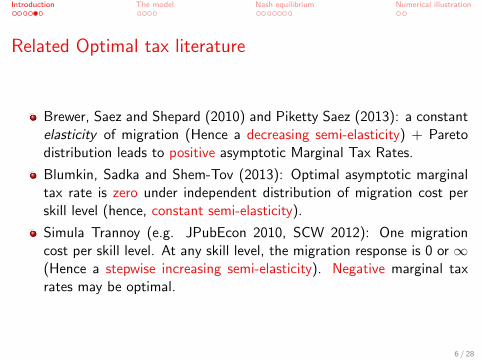
Brewer, Saez and Shepard (2010) and Piketty Saez (2013): a constantelasticity of migration (Hence a decreasing semi-elasticity) + Paretodistribution leads to positive asymptotic Marginal Tax Rates.

Blumkin, Sadka and Shem-Tov (2013): Optimal asymptotic marginaltax rate is zero under independent distribution of migration cost perskill level (hence, constant semi-elasticity).

Simula Trannoy (e.g. JPubEcon 2010, SCW 2012): One migrationcost per skill level. At any skill level, the migration response is 0 or ∞(Hence a stepwise increasing semi-elasticity). Negative marginal taxrates may be optimal.

6 / 28

Introduction The model Nash equilibrium Numerical illustration

Outline of the talk

1 The model.

2 Analytical Results.

3 Numerical Illustration of the Results.

7 / 28

Introduction The model Nash equilibrium Numerical illustration

The model

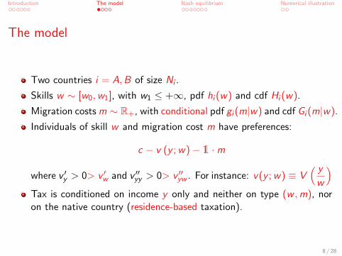
Two countries i = A,B of size Ni .

Skills w ∼ [w0,w1], with w1 ≤ +∞, pdf hi (w) and cdf Hi (w).

Migration costs m ∼ R+, with conditional pdf gi (m|w) and cdf Gi (m|w).

Individuals of skill w and migration cost m have preferences:

c − v (y ;w)− 1 ·m

where v ′y > 0> v ′w and v ′′yy > 0> v ′′yw . For instance: v(y ;w) ≡ V( yw

)Tax is conditioned on income y only and neither on type (w ,m), noron the native country (residence-based taxation).

8 / 28

Introduction The model Nash equilibrium Numerical illustration

Migration decisions

An individual of skill w and migration cost m, born in country A:

She gets UA(w) if she stays in country A.She gets UB(w)−m if she move to country B.She migrates to B if and only if m < UB(w)− UA(w).The mass of movers of skill w is GA (UB(w)− UA(w)|w) hA(w) NA.

Mass of residents in country A for ∆ = UA(w)− UB(w):

ϕA (∆;w) ≡ (1− GA (−∆|w)) hA(w) NA︸ ︷︷ ︸Non migrants in A

+ GB (∆|w) hB(w) NB︸ ︷︷ ︸Migrants from B

We assume m ∼ R+, so for each skill level w , there are workers forwhich migration is not an option and ϕA(·;w) > 0

9 / 28

Introduction The model Nash equilibrium Numerical illustration

Migration decisions (2)

Definition (Semi-elasticity of migration)

ηi (w ; ∆) ≡ 1

ϕi (∆;w)

∂ϕi (∆;w)

∂C (w)

= Percentage change in the density of taxpayers with skill w when theirconsumption C (w) is increased by $1.

Definition (Elasticity of migration)

νi (w ; ∆) ≡ Ci (w)

ϕi (∆;w)

∂ϕi (∆;w)

∂Ci (w)= Ci (w)× ηi (w ; ∆)

νi (w) can be increasing in w while ηi (w) may be decreasing.

10 / 28

Introduction The model Nash equilibrium Numerical illustration

The government

Governments are benevolent and Maximin (Rawlsian).

Exogenous budget requirement E ≥ 0.

The worst-off are non-migrants of productivity w0 (because of the sup-port of migration cost).

Government A takes TB(.) as given.

11 / 28

Introduction The model Nash equilibrium Numerical illustration

Nash Equilibrium (Not Necessarily Symmetric)

For country i , let f ∗(.)def≡ ϕi (U

∗i (w)−U∗−i (w);w) and η∗(w) = ηi (U

∗i (w)−

U∗−i (w);w).

Proposition 1: Optimal marginal tax under tax competition

T ′ (Y (w))

1− T ′ (Y (w))=α (w)

ε (w)︸ ︷︷ ︸Intensive

1− F ∗(w)

w f ∗(w)︸ ︷︷ ︸Distribution

(1− Ef ∗ [T (Y (x)) η∗(x) |x ≥ w ])︸ ︷︷ ︸Decrease of tax liabilities above Y (w)

Ef ∗ [T (Y (x)) η∗(x) |x ≥ w ] = Ef ∗

[T (Y (x))

Y (x)− T (Y (x))ν∗(x) |x ≥ w

]

12 / 28

Introduction The model Nash equilibrium Numerical illustration

The “Tiebout” best

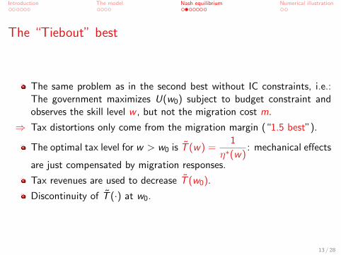
The same problem as in the second best without IC constraints, i.e.:The government maximizes U(w0) subject to budget constraint andobserves the skill level w , but not the migration cost m.

⇒ Tax distortions only come from the migration margin (“1.5 best”).

The optimal tax level for w > w0 is T̃ (w) =1

η∗(w): mechanical effects

are just compensated by migration responses.

Tax revenues are used to decrease T̃ (w0).

Discontinuity of T̃ (·) at w0.

13 / 28

Introduction The model Nash equilibrium Numerical illustration

The Tiebout best as a “target” for the second best

Optimal marginal tax rates are given by: Formula

T ′ (Y (w))

1− T ′ (Y (w))=α (w)

ε (w)

∫∞w

[T̃ (x)− T (Y (x))

]η∗(x) f ∗(x) dx

w f ∗(w)

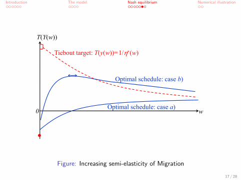
The second best consists in “smoothing” the Tiebout best (Jacquet et alii(2013)) to have tax liabilities as close as possible to the Tiebout target to

minimize distortions along the migration margin (lower∣∣∣T̃ (x)− T (Y (x)

∣∣∣).

14 / 28

Introduction The model Nash equilibrium Numerical illustration

T(Y(w))

Tiebout target: T(Y(w))=1/η∗

w0

Optimal schedule

Figure: Constant Semi-Elasticity of Migration

15 / 28

Introduction The model Nash equilibrium Numerical illustration

T(Y(w)) Tiebout target: T(y(w))=1/η∗(w)

Optimal schedule

w0

Figure: Decreasing Semi-Elasticity of Migration

16 / 28

Introduction The model Nash equilibrium Numerical illustration

T(Y(w))

Tiebout target: T(y(w))=1/η∗(w)

Optimal schedule: case b)

w0Optimal schedule: case a)

Figure: Increasing semi-elasticity of Migration

17 / 28

Introduction The model Nash equilibrium Numerical illustration

T(Y(w))

Optimal schedule

w0

Optimal schedule

Tiebout target: T(y(w))=1/η∗(w)

Figure: The semi-elasticity of Migration increases to infinity

18 / 28

Introduction The model Nash equilibrium Numerical illustration

Parameters

Constant labor supply elasticity c −( yw

)1+ 1ε , with ε = 0.25.

We use the CPS 2007 distribution of earnings for singles without kids.

The skill distribution is recovered using the federal and Californianincome tax schedules for singles without dependent.

Following Diamond (1998), Saez (2001), we extend the obtained ker-nel estimation by a truncated Pareto distribution (+ a mass at w1 =$1 534 6660).

⇒ The top 1% gets a fraction 17.6% of total income in our economy,instead of 18.3% (Alvarado, Atkinson, Piketty and Saez (2013)).

Public expenditures E are kept at their initial level $18, 157, whichrepresents 33.2% of total gross earnings of singles without kids.

3 different scenarios for η(w) = g (0|w) where the elasticity of migra-tion within the top 1% is on average 0.25.

19 / 28

Introduction The model Nash equilibrium Numerical illustration

Numerical illustration of the results

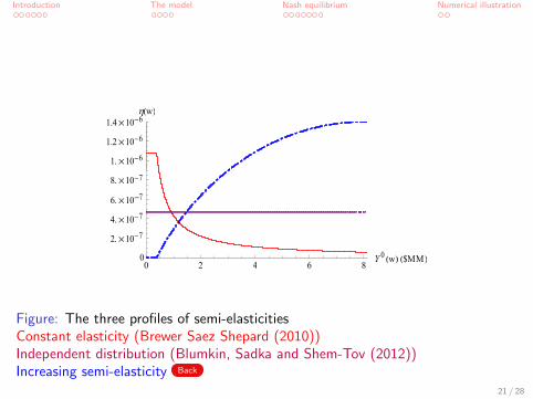
Consider 3 US economies that are identical but their migration re-sponses.

Identical mean elasticity of migration among the top 1% (0.25) but 3different scenarios for how the semi-elasticity varies. The 3 illustrative scenarios

⇒ Numerical illustration: Optimal Marginal Tax Rates Optimal Tax levels

Welfare Losses and Gains from tax competition

The empirical literature should not only estimate the elasticity of mi-gration among the top 1%.

We also need to know how the semi–elasticity of migration is changingalong the skill/income distribution.

20 / 28

Introduction The model Nash equilibrium Numerical illustration

1.µ10-6

1.2µ10-6

1.4µ10-6hHwL

0 2 4 6 8Y 0 HwL H$MML0

2.µ10-7

4.µ10-7

6.µ10-7

8.µ10-7

Figure: The three profiles of semi-elasticitiesConstant elasticity (Brewer Saez Shepard (2010))Independent distribution (Blumkin, Sadka and Shem-Tov (2012))Increasing semi-elasticity Back

21 / 28

Introduction The model Nash equilibrium Numerical illustration

0.15

0.20

0.25

0.30nHwL

0 20 40 60 80 100FHwL H%L

0.05

0.10

0.15

Figure: The three profiles of elasticitiesConstant elasticity (Brewer Saez Shepard (2010))Independent distribution (Blumkin, Sadka and Shem-Tov (2012))Increasing semi-elasticity Back

22 / 28

Introduction The model Nash equilibrium Numerical illustration

60

80

100

T 'HYL

1 2 3 4 5Y0

20

40

Figure: Optimal marginal tax ratesConstant elasticity (Brewer Saez Shepard (2010))Independent distribution (Blumkin, Sadka and Shem-Tov (2012))Increasing semi-elasticity Back

23 / 28

Introduction The model Nash equilibrium Numerical illustration

3

4THYL H$MML

0 1 2 3 4 5Y H$MML0

1

2

Figure: Optimal tax liabilitiesConstant elasticity (Brewer Saez Shepard (2010))Independent distribution (Blumkin, Sadka and Shem-Tov (2012))Increasing semi-elasticity Back

24 / 28

Introduction The model Nash equilibrium Numerical illustration

50

60

70

T HY L

YH%L

0 1 2 3 4 5Y H$MML20

30

40

50

Figure: Optimal average tax ratesConstant elasticity (Brewer Saez Shepard (2010))Independent distribution (Blumkin, Sadka and Shem-Tov (2012))Increasing semi-elasticity Back

25 / 28

Introduction The model Nash equilibrium Numerical illustration

102

104

106UHwLêU closed HwL H%L

20 40 60 80 100FHwL H%L

94

96

98

100

Figure: Welfare gains and losses from tax competitionConstant elasticity (Brewer Saez Shepard (2010))Independent distribution (Blumkin, Sadka and Shem-Tov (2012))Increasing semi-elasticity Back

26 / 28

Introduction The model Nash equilibrium Numerical illustration

300

350

400UHwLêU closed HwL H%L

99.0 99.2 99.4 99.6 99.8 100.0FHwL H%L100

150

200

250

Figure: Welfare gains and losses from tax competition in the top 1%Constant elasticity (Brewer Saez Shepard (2010))Independent distribution (Blumkin, Sadka and Shem-Tov (2012))Increasing semi-elasticity Back

27 / 28

Introduction The model Nash equilibrium Numerical illustration

Conclusion

With a numerical example. 3 economies that are identical, includingmean migration elasticity among the top 1% but different profiles ofthe migration responses have very different optimal tax policies.

A challenge of empirical research: investigating how migration re-sponses are changing within the top 1%.

28 / 28