
Tax collection, the informal sector, and productivity ...mkredler/ReadGr/GonzalezOnOrdonez14.pdf ·...
37
Tax collection, the informal sector, and productivity. Review of Economic Dynamics (2014) Julio César Leal Presented by Beatriz González Macro reading Group - May 2017
Transcript of Tax collection, the informal sector, and productivity ...mkredler/ReadGr/GonzalezOnOrdonez14.pdf ·...

Tax collection, the informal sector, andproductivity.
Review of Economic Dynamics (2014)
Julio César Leal
Presented by Beatriz GonzálezMacro reading Group - May 2017

Outline of this talk
Motivation
Empirical Evidence
Baseline Model
Decomposing the gains from enforcement
Monopolistic Competition
Conclusion

Outline of this talk
Motivation
Empirical Evidence
Baseline Model
Decomposing the gains from enforcement
Monopolistic Competition
Conclusion

Motivation
Informal SectorSector which encompasses all jobs which are not recognized as normal incomesources, and on which taxes are not paid.
Is the informal sector good or bad for the economy?
I Good. It allows firms to operate more efficiently. (Schneider and Enste2002)
I Bad. Incomplete enforcement of taxes: a)Distorts the natural competitiveprocess (Lewis 2004); b) Inefficient scale of operation (Farrell 2004).
This paper: It depends! Inverted U-shaped relationship bewteen output andenforcement.

Aim of this paper
I Assess quantitative effects of incomplete tax enforcement on aggregateoutput and productivity using a dynamic general equilibrium framework.
I Study gains from full enforcement from different set-ups:I Free entry to determine the endogenous mass of firms (Restuccia and Rogerson
2008)I Occupational choices (Gollin 1995, Guner et al. 2008)I Linkages and complementarities with monopolistic competition (Hsieh and
Klenow 2007, Jones 2011).
I Why?I Decompose the gains from full enforcement.I Compare quantitative results of different modelling assumptions.

Outline of this talk
Motivation
Empirical Evidence
Baseline Model
Decomposing the gains from enforcement
Monopolistic Competition
Conclusion

Empirical Evidence
I Data for Mexico:I ENOE (household survey) .I Economic Census + ENAMIN (household survey).
I Informal sector is large, and these establishments are small.I Around 44.5% to 50% of employees are informal in Mexico.
I Employment distribution has a ’missing middle’, and labor is concentrated insmall establishments.I Suggestive evidence that informality is the driving force.
266 J.C. Leal Ordóñez / Review of Economic Dynamics 17 (2014) 262–286
Table 2Employment distribution: Mexico vs. the US.
Size category US Mexico Mex-Formal-1 Mex-Formal-2 Mex-Informal-2
Under 20 25.0 57.3 24.8 29.2 89.120 to 99 29.8 13.0 21.3 30.8 7.9100 or more 45.3 29.8 53.9 40.0 3.0
Mean size 17 5.5 – – –
Sources: For the US, the Census Bureau’s County Business Patterns (2003). For Mexico, the INEGI, using the census+ENAMIN data (2008). For Mex-Formal-1,the IMSS records (2008). For Mex-Formal-2 and Mex-Informal-2, the ENOE (2008 Q2). The mean size for the US is taken from Guner et al. (2008), whilethe mean size in Mexico corresponds to the census + ENAMIN data.
literature, known as the “missing middle” (see Tybout, 2000 for a survey of developing countries). This phenomenon is alsoreflected in the mean size of establishments. In Mexico, the mean size is 5.5 workers, while in the US it is 17 workers (seealso the last row of Table 2).
In the third column of Table 2, I present the distribution of employment in Mexico’s formal sector. To do so, I usedata from the IMSS records. Notice that the IMSS records do not include information on the informal sector. Notice alsothat the distribution of the Mexico’s formal sector is very similar to that in the US. This suggests two things: (1) that theinformal sector is the main driver of the “missing middle” phenomenon, and (2) that most informal employees work insmall establishments or that informal establishments are small.
The size distribution of employment in the formal sector can also be obtained from the ENOE. In the case of the ENOE,the survey also includes information on the employment distribution of informal workers. Both distributions are presentedin the last two columns of Table 2. The broad picture is similar to what we see using the IMSS records: most informalemployees are working in small establishments and the distribution within the formal sector is similar to that in the US.See Appendix A for a detailed description of these distributions.
2.3. Capital distortions
It is a well-established fact that informal firms operate with low capital per worker. For example, Thomas (1992) re-ports this for a survey of Peruvian establishments, de Paula and Scheinkman (2007) make the case for Brazilian firms, andDi-Giannatale et al. (2011) for Mexico. However, my interest is on the particular shape of the capital distortions sufferedby informal establishments. To investigate this, I use data from the ENAMIN, a survey that captures a large proportion ofinformality because its focus is on businesses with 6 or fewer workers (including the owner).
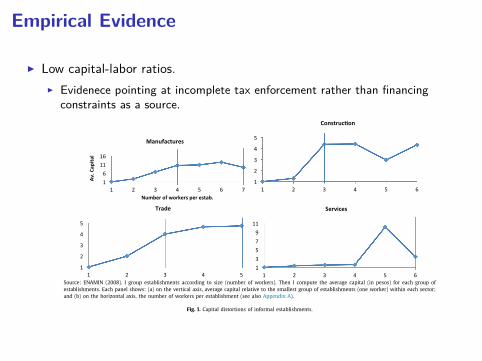
Fig. 1 plots the capital (on the y-axis) and labor (on the x-axis) of informal establishments.5 There are four panels show-ing different sectors covered by the ENAMIN. In a typical model of heterogeneous firms without distortions, the capital–laborratio is constant across size; this implies a linear relationship in a plot of capital vs. labor. Notice, however, that the rela-tionship between capital and labor in Fig. 1 is nonlinear; in particular, there is a range of labor for which capital is constant.This range varies slightly from sector to sector, but is present in all. In other words, there is a capital level that infor-mal establishments do not exceed. Also notice that this distortion on capital translates into low capital–labor ratios, as theliterature reports.
This type of distortion can be rationalized in a model in which the probability of being caught evading taxes increaseswith capital. In particular, assume that the probability of detection is zero if capital is less than or equal to a certain value,b > 0, and one if not. This introduces an incentive to remain small and to operate in the informal sector, hiring no morethan b units of capital in order to benefit from tax evasion.
An alternative interpretation is that low capital–labor ratios reflect the borrowing constraints faced by informal en-trepreneurs. Under this view, these individuals do not have access to formal credit because they lack the collateral neededto take out a loan. Since loans are used to finance capital, borrowing-constrained individuals operate with low capital.
2.4. Financial constraints or incomplete tax enforcement?
In the ENAMIN (2008), there is information that suggests that informal firms are not financially constrained. In thesurvey, the owners are asked how they financed their start-up costs: 50.5% stated that they used their own savings; 19.4%said they borrowed from friends or relatives at zero interest; 13.5% stated that they did not need financing; 4.2% said theyused a severance payment from a former job; and 2.2% used trade credit. Only 1.2% used credit from commercial banks.As discussed in Kaplan et al. (2007), this may mean that access to credit is difficult for small firms, or alternatively, thatdemand for credit is low. Fortunately, a second question in the ENAMIN is enlightening: the owners are asked what the mainproblem faced by their business is; only 2.39% answered that lack of credit was a problem; in contrast, 45% answered that
5 I use the following definition: formal if the business issues invoices, informal if not. In order to use invoices, the business must be registered with thetax authority.
Empirical Evidence
I Low capital-labor ratios.I Evidenece pointing at incomplete tax enforcement rather than financing
constraints as a source.J.C. Leal Ordóñez / Review of Economic Dynamics 17 (2014) 262–286 267
Source: ENAMIN (2008). I group establishments according to size (number of workers). Then I compute the average capital (in pesos) for each group ofestablishments. Each panel shows: (a) on the vertical axis, average capital relative to the smallest group of establishments (one worker) within each sector;and (b) on the horizontal axis, the number of workers per establishment (see also Appendix A).
Fig. 1. Capital distortions of informal establishments.
low sales and excessive competition were the main problem, and 18% said that they had no problems. Therefore, informalentrepreneurs seem to be unaffected by credit constraints.
This evidence supports the research of Moll (2010), who argues that capital misallocation induced by borrowing con-straints can be undone through self-financing because “. . . an entrepreneur without access to external funds can stillaccumulate internal funds over time to substitute for the lack of external funds.”6
Therefore, if financial frictions do not induce capital misallocation, then why do we see distortions in the capital–laborratios of informal firms? I argue that the way taxes are enforced in developing countries induces these distortions on capital.I start with the observation that large establishments are more visible to tax authorities. In fact, a probability of detectionthat increases with firm size is a common assumption in the informal-sector literature.7 Ihrig and Moe (2001) argue thatcapital in particular is harder to hide. Their empirical work on Asian economies shows that a rise in an index of taxenforcement is more effective in manufacturing than in services: manufacturing requires physical equipment and structures,whereas activities in the service sector are easier to hide. Following on from this idea, if the probability of detection dependson capital, we should see a larger proportion of informality in sectors that are less capital intensive. We can corroboratethis using the ENOE: the proportion of informal employees in the trade sector is 53%, while in manufacturing it is 31%.
I also argue that the specific shape of the probability of detection is close to a step function: zero if capital is less than orequal to b > 0, and one if not. Although this assumption proves to be not crucial for the quantitative results, it is motivatedby the following observations: (1) virtually no small businesses in the ENAMIN report taxes being a problem, whilst only0.41% said that they were; (2) the majority of these businesses are not registered with any tax or municipal authority, whichsuggests that they are facing a probability of detection close to zero and explains why taxes are not a concern for thesefirms; (3) Fig. 1 shows that capital flattens out for a certain labor range, consistent with the incentives of the step function.
Moreover, the research of Bigio and Zilberman (2011) favors the step function. The authors study the optimal monitoringstrategy of a tax authority that maximizes revenue and faces a limited amount of resources, as well as costly monitoring.They show that when the tax authority screens observable inputs (such as capital, labor or land), the optimal strategy is abang–bang solution: monitor small firms with zero probability up to a threshold and large firms with the highest possibleprobability. Moreover, the authors emphasize that the optimal policy in their paper is consistent with three empirical regu-larities: (1) the presence of a “missing middle” (Tybout, 2000); (2) an inverse relationship between the amount evaded andthe size of the firm (Dabla-Norris et al., 2008); and (3) some evaders producing inefficiently (La Porta and Shleifer, 2008).In addition to these three, I argue that when the probability of detection depends on observable capital, the model is alsoconsistent with a fourth regularity: (4) informal firms exhibit a size range for which capital is constant (Fig. 1).
In the baseline model, I assume that the probability of being caught depends on capital and takes the form of a stepfunction. In Appendices A–C, I also explore how the quantitative results change if a continuous probability is assumed.
6 This possibility depends crucially on the evolution of the entrepreneur’s productivity over time. Moll shows that contrasting results in previous worksin the literature on financial constraints and capital misallocation can be explained by differences in the assumption of the persistence of the productivityshock. Buera et al. (2011) and Midrigan and Xu (2010) are two examples with contrasting results.
7 See for example, Rauch (1991), Fortin et al. (1997) and, more recently, de Paula and Scheinkman (2007).

Outline of this talk
Motivation
Empirical Evidence
Baseline Model
Decomposing the gains from enforcement
Monopolistic Competition
Conclusion

Baseline Model
I Discrete time, one representative household populated by a continuum ofindividuals.
I Heterogeneous on ability z ∈ [z, z].
I 1 unit of time per period.
I Decreasing returns to scale technology: θk + θl < 1.
Formal entrepreneur
πF(z;w, r) = max{lF,kf}
(1− τy)zkθk
F lθl
F −wlF − rkF (1)
I Government tax to output: τy

Baseline Model
Informal entrepreneur
πI(z;w, r) = max{lI,kI}
(1− p(kI))zkθk
I lθl
I −wlI − rkI (2)
I Enforcement function
p(kI) =
{0 if k(z) 6 b1 else
I No one gets caught in equilibrium!
EmployeeI Receive wage w.

Representative Household
max{Ct,Kt,It(z),Ft(k)}
∞∑t=0
βtu(Ct) (3)
s.t.Ct + Kt+1 − (1− δ)Kt = rtKt + E(wt, rt; τy,b) + Tt , ∀t (4)
where earnings are
E(w, r) =∫ zz
I(z)πI(z;w, r)dG(z) +∫ zz
F(z)πF(z;w, r)dG(z) +∫ zz
(1− I(z) − F(z))wdG(z)
(5)Aggregation and Definition of Equilibrium

Properties of the modelOccupational Choice
270 J.C. Leal Ordóñez / Review of Economic Dynamics 17 (2014) 262–286
Fig. 2. Characterization of occupational decisions. (For interpretation of the references to color in this figure, the reader is referred to the web version ofthis article.)
I focus on the steady-state (SS) equilibrium of this economy. As is standard, the first-order conditions of this problem inthe steady state imply that:
r = 1β
− (1 − δ). (9)
3.4. Market clearing
The market-clearing condition for the labor market will equate the aggregate labor demand from the two sectors to thelabor supply:
z!
z
I(z; wt, rt)lI (z; wt, rt)dG(z) +z!
z
F (z; wt, rt)lF (z; wt, rt)dG(z) =z!
z
W (z; wt, rt)dG(z), (10)
where W (z; wt , rt) = 1 − I(z; wt , rt) − F (z; wt , rt). Market clearing for the capital and good markets are, respectively:
z!
z
I(z; wt, rt)kI (z; wt, rt)dG(z) +z!
z
F (z; wt, rt)kF (z; wt, rt)dG(z) = Kt,
and
Ct + Kt+1 − (1 − δ)Kt =z!
z
I(z; wt, rt)yI (z; wt, rt)dG(z) +z!
z
F (z; wt, rt)yF (z; wt, rt)dG(z).
3.5. Equilibrium definition
An equilibrium for this economy is sequences {Ct , Kt+1, wt , rt} and {It(z), Ft(z)} ∀z ∈ [z, z], whereby taking factor prices{wt, rt}, policies parameters τy and b, and transfers {Tt}, the household solves its problem, firms maximize their profits ∀t ,and markets clear ∀t .
3.6. Steady state
In the following section, I will focus on the steady-state equilibrium. Since I define time-invariant taxation and enforce-ment policies, the dynamic part of this economy is no different from that in the standard growth model. In the steady state,factor prices, occupational decisions, aggregate capital and output are constant over time.
4. Properties of the model
4.1. Occupational choices
In this section, I analyze a number of properties of the model. The steady-state equilibrium is characterized by threethresholds, {z1, zc, z2}, which summarize the occupational decisions of the agents and whether the capital choices of infor-mal entrepreneurs are constrained or unconstrained. Fig. 2 provides a graph of the optimal occupational choices. I study thedetermination of these thresholds next.
I Occupational choice depends on ability z.

Properties of the modelCapital-labor choice
272 J.C. Leal Ordóñez / Review of Economic Dynamics 17 (2014) 262–286
Fig. 3. Capital profile. Fig. 4. Capital–labor ratios.
are positive, it must follow that the more capable informal entrepreneurs are constrained. To illustrate this, consider theentrepreneur z2, who is indifferent between the two sectors. If informal, she would hire b capital; if formal, she wouldhire an amount strictly greater than b. To see why, note that optimal decisions of formal entrepreneur z2 are the same asthose of a hypothetical entrepreneur that operates unconstrained and pays no taxes; this entrepreneur is zh = (1 − τy)z2.Entrepreneur z2 hires capital strictly greater than b as long as zh > zc , and this inequality holds, because, as shown in thebottom case of Eq. (14), πI (z; w, r) is strictly increasing.
Notice that, as a corollary of this property, the labor demand schedule is strictly increasing with respect to z, in equilib-rium. Finally, notice that the discontinuity in the capital schedule translates into an informal sector that appears less capitalintensive. The capital–labor ratio is smaller for constrained establishments (see Fig. 4), as is the capital–output ratio.
5. Calibration
My calibration strategy is different from that followed in works that focus on developed economies, such as Restucciaand Rogerson (2008) and Guner et al. (2008). These papers assume that the US has small distortions and the distortion-freescenario in the model is used as a benchmark to study how deviations affect equilibrium variables. In this study, however,the distortions characteristic of the Mexican economy prevent me from taking the same approach.
The parameters to calibrate are the tax rate paid by the formal sector, τy , the technology parameters, θk , γ , and depre-ciation δ, the discount rate β , the enforcement policy parameter, and the entrepreneurial ability distribution parameters.The enforcement policy used as a benchmark is described in Eq. (2), where the probability of detection depends on capital;therefore, only one parameter needs to be calibrated, i.e., b. Entrepreneurial ability is assumed to follow a truncated Paretodistribution with parameters zmin, zmax, and s. More specifically, I assume that z has CDF:
G(z) = 1 −! zmin
z
"s
1 −! zmin
zmax
"s ,
where s > 0 is the shape parameter and z ∈ [zmin, zmax], with 0 < zmin < zmax. I make this choice for two main reasons.The first is that the firm-size distribution in the US has been reported to be well-described by a Pareto distribution (Axtell,2001). The second is more practical: a truncated Pareto is fully defined on an interval that I can link directly to the modelobjects z and z.
Next, I continue with the value of the parameters for which I am able to provide an independent calibration: the ex-ponent of capital in the production function θk , the depreciation rate δ, and the tax rate τy . I choose θk = 0.33 for thefollowing reasons: first, because it is the standard value used by a number of studies focusing on Mexico; for example,Bergoeing et al. (2001) use θk = 0.33 to compute TFP series for Mexico, Solimano et al. (2005) perform growth accountingusing θk = 0.35 for several Latin American economies including Mexico, and Restuccia (2008) uses a value of θk = 0.28 fora production function with decreasing returns to scale; second, this value is consistent with the estimates of Garcia-Verdu(2005). I choose δ = 0.05 following Solimano et al. (2005) and Bergoeing et al. (2001), who use the same value for thedepreciation rate in articles using Mexican data; additionally, as I will explain below, this value is roughly consistent withdata on investment and on consumption of fixed capital in Mexico. To calibrate the tax rate, an assessment of the fiscalburden on formal firms is needed. I take the total tax revenue from the formal sector, which amounted to 11% of GDP in2008; then, I make an assessment of the value added associated to these firms, this value amounts to 44% of GDP.9 Theratio of these two numbers is τy = 11/44 = 0.25.
9 The value added by the formal sector consists of the value added by financial corporations (3.5%), the value added by public non-oil, non-financialcorporations (2%), the value added by the general government (8%), and the value added by formal private non-financial corporations and quasi-corporations(30.5%).
I z1 < z < zc: Informal firm operates unconstrained: kI(z,w, r) < b.I zc < z < z2: Informal firm operates constrained, kI(z,w, r) = b.
Calibration

Baseline ExperimentsShort term effects
Experiment: Introduce full tax enforcement by making b = 0 → All firms payτy.
Short term effects. Maintain K fixed.J.C. Leal Ordóñez / Review of Economic Dynamics 17 (2014) 262–286 275
Table 5Parameter values.
Parameter Calibrated value
θk 0.33δ 0.05β 0.94γ 0.76zmin 1zmax 13.05s 4.25b 10.50τy 0.25
Table 6Short-run effects: First period after change in enforcement.
Variable Value under complete enforcementrelative to benchmark
Y 1.044τy 1K 1TFP 1.044L 1.120µ 2.104r 1.130w 0.829
decreasing returns and the more efficient it is to concentrate production in large establishments. In the limiting case ofγ = 1 (constant returns to scale), efficient output is reached by concentrating all resources in a single unit, i.e., the mostproductive one. The low value of γ I find implies that the distortion-free allocation for Mexico is to have more workers insmall units than would be the case in countries where the degree of decreasing returns is smaller (i.e., a larger γ ).
That the distortion-free allocation in Mexico is different than that in the US is not necessarily a bad result. It is not thethesis of this paper that the differences between Mexico and US distributions are due solely to tax enforcement differences.It could be argued that Mexico’s distortion-free skewed distribution is merely the result of its early stage of development.A number of authors have documented the steady rise in average firm size in the US during the 19th and 20th century (fora short bibliography, see Desmet and Parente, 2009). Furthermore, when one looks at the distribution of US of the past, at apoint in time during which the US had the same GDP per capita as modern-day Mexico (around the 1930s), it is clear thatit was not as highly concentrated in small establishments as it is in today’s Mexico.12
Finally, one more feature of the calibrated economy is that all informal entrepreneurs are constrained (i.e. that zc ≈ z1),which is roughly consistent with the evidence in Fig. 1.13
6. Results of the baseline model
Once the model is calibrated to the Mexican economy, I can investigate the effects of incomplete enforcement policies.To do this, I use this calibrated economy as a benchmark and perform three exercises: one that focuses on short-run effectsand two more that explore long-run effects. In these exercises, I introduce complete tax enforcement by making b = 0 inthe model; this implies that all establishments would pay a uniform tax (τy).
As a first step, I look at the equilibrium in the first period, immediately after the new enforcement policy is introduced.In this period, the capital stock is the same as in the economy with incomplete enforcement, because accumulation has notoccurred yet. Table 6 shows the value of aggregate variables in this context. Since capital and employment (employees +entrepreneurs) are no different from the benchmark economy, the only reason that output increases is that these resourcesare used more efficiently. Not surprisingly, output increases proportionally with TFP. Also, notice that in this first period,wages decrease.
The gains in TFP are associated with the removal of the distortions present under incomplete tax enforcement. The effectsof incomplete enforcement include distorting three margins: optimal occupational choices, allocation of resources acrossestablishments, and the capital–labor ratios of informal establishments. The first two distortions occur across establishments,while the last occurs within establishments. Incomplete tax enforcement distorts occupational choices because it makesentrepreneurship more attractive; furthermore it distorts the allocation of resources directly because it makes it possible tohave some establishments paying taxes and some others not; finally, it distorts the capital–labor ratio of a group of informalestablishments, because this is the optimal response to a probability of detection that increases with capital.
The short-run gains in TFP respond to the elimination of the distortions mentioned above. Note first, that the em-ployee/entrepreneur threshold z1 increases because a group of low-ability individuals no longer find it attractive to beentrepreneurs, so the average ability in the economy (µ in Table 6) improves14; second, note that since every establishmentpays the same tax rate, marginal products are equalized and the allocation of resources improves; and finally, note thatsince the probability of detection plays no important role under full enforcement, capital–labor ratios become undistorted.
In Table 6, it can be confirmed that, as a result of the change in threshold z1, the proportion of employees in theeconomy increases by 12% and the average ability by 110%. Note that consistent with this, wages decline to a level that is0.83 of the benchmark level. Also note that the rental rate of capital increases by 13% in this first period.
12 Granovetter (1984) documented the fact that the proportion of employees in US manufacturing establishments with fewer than 20 employees was 10%in 1933, while the proportion of employees in Mexican manufacturing establishments with fewer than 15 workers was 37.5% in 2005. Notice that the sizecategory is capped at a smaller size for Mexico than for the US, but the proportion allocated is still larger. Similarly, for the same size categories I find thatfor the retail and wholesale sectors, the figures are 63.8% and 44.4% for the US in 1939, and 72% and 48% for Mexico in 2005.13 This is clearer for construction, trade and services, which are the sectors where most of the informal entrepreneurs operate.14 This also entails a reduction in the mass of firms which reduces output, see Section 7 for a decomposition of the gains.
Gains from improvement in:I Optimal occupational choices.I Allocation of resources across establishments.I Capital-labor ratios of informal establishments.

Baseline ExperimentsLong term effects
I With full enforcementI Occupational choices and allocation of resources across establishments are
same as if τy = 0.
Long term effects. Full tax enforcement (b = 0)J.C. Leal Ordóñez / Review of Economic Dynamics 17 (2014) 262–286 277
Table 7Comparison across steady states with a constant tax rate.
Variable Value under complete enforcementrelative to benchmark
Y 1.109τy 1K 1.200TFP 1.044L 1.120µ 2.104w 0.88
Table 8Comparison across steady states with constant revenue.
Variable Value under complete enforcementrelative to benchmark
Y 1.193τy 0.52K 1.498TFP 1.044L 1.120µ 2.104w 1.10
Fig. 7. Partial enforcement.
In Table 8, I present the effects of such an exercise on the steady-state values. If Mexico’s present enforcement policywere complete, it would be able to reduce taxes to 52% of the current levels. This tax reduction gives an extra boost to theeconomy. Overall, output would increase 19%. The table shows that this increase would be driven mainly by a 50% increasein capital accumulation, while TFP would play a smaller role, with an increase of 4.4% which occurs fully in the short run.In the long run, once accumulation of capital takes place, labor productivity is increased and the wage rate rises to a levelthat is 10% higher than the benchmark.
6.1. Partial enforcement
Full enforcement corresponds to an extreme policy change; one interesting question is, what are the gains from partialimprovements in enforcement? After all, many developed countries do not enforce taxes fully.
In Fig. 7, partial enforcement is achieved by moving the parameter b over a range that goes from 0.1 to 2.5 times itscalibrated value. Panel (a) of Fig. 7 plots output vs. the size of the informal sector; panel (b) output vs. enforcement; andpanel (c) enforcement vs. the size of the informal sector. In the figure, output is measured relative to the benchmark andenforcement is measured by b, which represents the value of the enforcement parameter relative to the calibrated value.Thus, in the benchmark b = 1. Furthermore, the benchmark values in each panel are indicated by a cross.
A few important points arise when analyzing this picture. First, note in panels (a) and (b) that the gains from en-forcement are nonlinear; in fact, starting at the benchmark, a marginal increase in enforcement (i.e., a reduction of b or,equivalently, a reduction in the informal sector) reduces output; second, it is not until b reaches 0.5 that we can see outputgains; third, as we further reduce b (from 0.5 to 0.25), output increases rapidly; finally, note that achieving the enforcementlevels of a developed country (i.e., 10% of informality) generates around 50% of the gains obtained under full enforcement.One reason behind this nonlinear result is the relationship between b and the size of the informal sector; note that the
I TFP does not increase further.I Capital accumulation increases by 20%.I No distortion in capital-labor → Increase MPK.
Baseline ExperimentsLong term effects
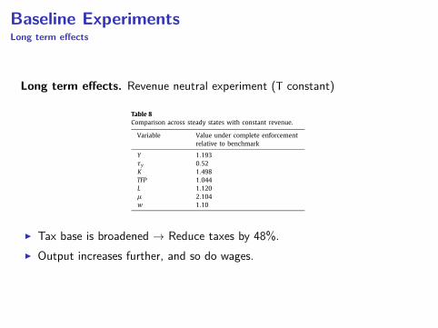
Long term effects. Revenue neutral experiment (T constant)J.C. Leal Ordóñez / Review of Economic Dynamics 17 (2014) 262–286 277
Table 7Comparison across steady states with a constant tax rate.
Variable Value under complete enforcementrelative to benchmark
Y 1.109τy 1K 1.200TFP 1.044L 1.120µ 2.104w 0.88
Table 8Comparison across steady states with constant revenue.
Variable Value under complete enforcementrelative to benchmark
Y 1.193τy 0.52K 1.498TFP 1.044L 1.120µ 2.104w 1.10
Fig. 7. Partial enforcement.
In Table 8, I present the effects of such an exercise on the steady-state values. If Mexico’s present enforcement policywere complete, it would be able to reduce taxes to 52% of the current levels. This tax reduction gives an extra boost to theeconomy. Overall, output would increase 19%. The table shows that this increase would be driven mainly by a 50% increasein capital accumulation, while TFP would play a smaller role, with an increase of 4.4% which occurs fully in the short run.In the long run, once accumulation of capital takes place, labor productivity is increased and the wage rate rises to a levelthat is 10% higher than the benchmark.
6.1. Partial enforcement
Full enforcement corresponds to an extreme policy change; one interesting question is, what are the gains from partialimprovements in enforcement? After all, many developed countries do not enforce taxes fully.
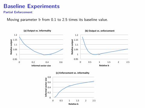
In Fig. 7, partial enforcement is achieved by moving the parameter b over a range that goes from 0.1 to 2.5 times itscalibrated value. Panel (a) of Fig. 7 plots output vs. the size of the informal sector; panel (b) output vs. enforcement; andpanel (c) enforcement vs. the size of the informal sector. In the figure, output is measured relative to the benchmark andenforcement is measured by b, which represents the value of the enforcement parameter relative to the calibrated value.Thus, in the benchmark b = 1. Furthermore, the benchmark values in each panel are indicated by a cross.
A few important points arise when analyzing this picture. First, note in panels (a) and (b) that the gains from en-forcement are nonlinear; in fact, starting at the benchmark, a marginal increase in enforcement (i.e., a reduction of b or,equivalently, a reduction in the informal sector) reduces output; second, it is not until b reaches 0.5 that we can see outputgains; third, as we further reduce b (from 0.5 to 0.25), output increases rapidly; finally, note that achieving the enforcementlevels of a developed country (i.e., 10% of informality) generates around 50% of the gains obtained under full enforcement.One reason behind this nonlinear result is the relationship between b and the size of the informal sector; note that the
I Tax base is broadened → Reduce taxes by 48%.I Output increases further, and so do wages.
Baseline ExperimentsPartial Enforcement
Moving parameter b from 0.1 to 2.5 times its baseline value.
J.C. Leal Ordóñez / Review of Economic Dynamics 17 (2014) 262–286 277
Table 7Comparison across steady states with a constant tax rate.
Variable Value under complete enforcementrelative to benchmark
Y 1.109τy 1K 1.200TFP 1.044L 1.120µ 2.104w 0.88
Table 8Comparison across steady states with constant revenue.
Variable Value under complete enforcementrelative to benchmark
Y 1.193τy 0.52K 1.498TFP 1.044L 1.120µ 2.104w 1.10
Fig. 7. Partial enforcement.
In Table 8, I present the effects of such an exercise on the steady-state values. If Mexico’s present enforcement policywere complete, it would be able to reduce taxes to 52% of the current levels. This tax reduction gives an extra boost to theeconomy. Overall, output would increase 19%. The table shows that this increase would be driven mainly by a 50% increasein capital accumulation, while TFP would play a smaller role, with an increase of 4.4% which occurs fully in the short run.In the long run, once accumulation of capital takes place, labor productivity is increased and the wage rate rises to a levelthat is 10% higher than the benchmark.
6.1. Partial enforcement
Full enforcement corresponds to an extreme policy change; one interesting question is, what are the gains from partialimprovements in enforcement? After all, many developed countries do not enforce taxes fully.
In Fig. 7, partial enforcement is achieved by moving the parameter b over a range that goes from 0.1 to 2.5 times itscalibrated value. Panel (a) of Fig. 7 plots output vs. the size of the informal sector; panel (b) output vs. enforcement; andpanel (c) enforcement vs. the size of the informal sector. In the figure, output is measured relative to the benchmark andenforcement is measured by b, which represents the value of the enforcement parameter relative to the calibrated value.Thus, in the benchmark b = 1. Furthermore, the benchmark values in each panel are indicated by a cross.
A few important points arise when analyzing this picture. First, note in panels (a) and (b) that the gains from en-forcement are nonlinear; in fact, starting at the benchmark, a marginal increase in enforcement (i.e., a reduction of b or,equivalently, a reduction in the informal sector) reduces output; second, it is not until b reaches 0.5 that we can see outputgains; third, as we further reduce b (from 0.5 to 0.25), output increases rapidly; finally, note that achieving the enforcementlevels of a developed country (i.e., 10% of informality) generates around 50% of the gains obtained under full enforcement.One reason behind this nonlinear result is the relationship between b and the size of the informal sector; note that the

Outline of this talk
Motivation
Empirical Evidence
Baseline Model
Decomposing the gains from enforcement
Monopolistic Competition
Conclusion
Decomposing the gains from enforcement
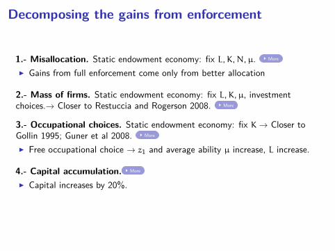
1.- Misallocation. Static endowment economy: fix L,K,N,µ. More
I Gains from full enforcement come only from better allocation
2.- Mass of firms. Static endowment economy: fix L,K,µ, investmentchoices.→ Closer to Restuccia and Rogerson 2008. More
3.- Occupational choices. Static endowment economy: fix K→ Closer toGollin 1995; Guner et al 2008. More
I Free occupational choice → z1 and average ability µ increase, L increase.
4.- Capital accumulation. More
I Capital increases by 20%.

Summary of decompositionJ.C. Leal Ordóñez / Review of Economic Dynamics 17 (2014) 262–286 279
Table 10Effects on factor levels.
Var. Bench. A. Free entry Occupational choices
B. Short run C. Long run
Y 1 0.925 1.044 1.109K 1 1 1 1.200L 1 1 1.120 1.120N 1 0.662 0.424 0.424µ 1 1 2.104 2.104TFP 1 0.925 1.044 1.044
Table 11Decomposing gains of perfect enforcement.
Var. A = MP equalization B = A + free entry C = A + occupational choice D = C + capital accumulation Total
Y 1.02 0.92 1.04 1.11(△Y ) +2 −10 +12 +7 +11TFP 1.02 0.91 1.04 1.04△TFP +2 −10 +12 0 +4
7.2. The mass of firms (adding free entry)
To investigate the importance of distortions in the mass of firms, I add a free-entry condition but keep the assumptions ofa fixed endowment of labor, a fixed endowment of capital, and a fixed average ability (i.e., I shut down occupational choicesand investments). This modification brings the model closer that used by Restuccia and Rogerson (2008) (group “a”).
Consider a potential entrepreneur that is evaluating whether to enter or not. This agent takes into account the expectedprofits of incumbent entrepreneurs. Thus, the value of entry is described by:
We =z!
z1
π(z)g(z)dz − ce,
where g(z) = g(z|z > z1)/(1 − G(z1)), ce is an entry cost, π(z) are profits, and z1 is given by w = πM(z1; w, r) (from thebenchmark, in the baseline model). Now let N be the mass of firms and E the endowment of labor; the labor marketclearing condition is as follows:
E = N
z!
z1
l(z)g(z)dz,
where E = 1 − G(z1).Notice that in this economy, average entrepreneurial ability is constant, independent of N , and is equal to µ =
" zz1
z1
1−γ g(z)dz. Given ce , I can find equilibrium allocations by solving the free entry and the labor market clearing con-
ditions for w and N . Column A in Table 10 shows the results.16
The introduction of complete enforcement reduces We because the expected value of incumbent entrepreneurs is hit byhigher taxes; therefore, the mass of firms is negatively affected. In Eq. (17), the mass of firms is an important component ofaggregate output, thus output decreases. We can perform the accounting of output losses using Eq. (17). Letting Y1 be thevalue of output in Table 9 and Y the corresponding value in Table 10, the effect of full enforcement under this exercise is:YY1
= 0.6620.24 ≈ 0.9251.023 ≈ 0.904. Thus, adding firm entry reduces output by 10% (see also Table 11).
7.3. Occupational choices
Now consider an economy with an occupational-choice rather than a free-entry condition, but keep the assumption of afixed capital stock. This brings the model closer to Gollin (1995) and Guner et al. (2008) (group “b”), and is also our baselinemodel in the short run. Adding occupational choices will bring good news, because it will allow the economy to increaseaverage ability and the supply of labor, while reducing entry.
Notice first that the introduction of full enforcement pushes z1 to the right. As a result, the mass of firms N = 1 − G(z1)is reduced; however, the average ability µ and the supply of labor F (z1) both increase. This exercise is identical to that
16 To obtain the value of ce , I use the fact that We must be zero in equilibrium (the free-entry condition) and set it equal to the value of" z
z1π(z)g(z)dz
in the benchmark.

Outline of this talk
Motivation
Empirical Evidence
Baseline Model
Decomposing the gains from enforcement
Monopolistic Competition
Conclusion

Adding Monopolistic Competition
I Change set-up to Monopolistic competition (Hsieh and Klenow 2007, Jones2011). More on Monopolistic Competition
I Amplifies the effects of resource misallocation through complementarityacross varieties.
282 J.C. Leal Ordóñez / Review of Economic Dynamics 17 (2014) 262–286
Table 12Complete enforcement with monopolistic competition.
Perfect competition Monopolistic competition
Fixed tax rate Revenue neutral Fixed tax rate Revenue neutral
Y 1.11 1.19 1.18 1.34K 1.20 1.50 1.27 1.70TFP 1.04 1.04 1.09 1.12
Table 13Summary of output-loss decomposition (%).
Discontinuous dist. Continuous dist. Relative Related paper
Total loss with fixed revenue −0.34 −0.24 0.70Total loss with fixed tax rate −0.18 −0.12 0.66Contribution of
factor misallocation 0.13 0.11 0.57firm entry −0.56 −0.39 0.46 RRoccupational choices 0.68 0.47 0.45 Gollin, GVXcapital accumulation 0.37 0.43 0.77complementarities 0.38 0.37 0.65 HK, Jones
9. Summary of the output-loss decomposition
Table 13 presents a summary of the decomposition of output losses. It presents this decomposition for both the discon-tinuous distortion analyzed here and a continuous distortion analyzed in Appendix C (see also Section 9.1). For the case ofthe step function (discontinuous distortion), the total loss is 18% when the tax rate is fixed; this, in turn, can be decomposedinto five sources: factor misallocation, firm entry, distortions of occupational choices, capital accumulation, and complemen-tarities. Pure factor misallocation contributes 13% to the output loss, firm entry −56%, occupational choices 68%, capitalaccumulation 37%, and complementarities 38%. Notice that informality has a positive effect on output because it providesan incentive to firm entry, so the increase in the mass of firms contributes −56% to the output loss. This is reversed by thecontribution of occupational choices, which increase average ability and labor supply, whilst reducing entry. Thus, the netcontribution of occupational choices and free entry is 12% (68–56%).
9.1. Discussion
A natural question that arises from this analysis is, what is the cost of increasing enforcement? These costs have to besubtracted from the output gains reported in the previous section, in order to provide a sense of the net gain associatedwith the policy change in question.
Since the informal sector consists of many small businesses, better enforcement increases the number of taxpayers overwhich the authorities need to provide surveillance. In the benchmark, there are 22 times more informal establishmentsthan formal establishments; in other words, informal establishments represent 95% of all entrepreneurs. According to offi-cial Mexican tax authority data, the office currently spends around 1 peso for every 100 pesos collected.19 We can use thisinformation to obtain the enforcement cost per establishment in the model and then calculate the cost of full enforcement,assuming that cost per establishment is a constant and taking into account the increase in the number of formal establish-ments. I calculate that introducing full enforcement will increase total enforcement costs by a factor of 9.6, a huge increase;however, it represents a small fraction of gross revenue. Gross revenue increases to 25% of the model’s GDP and enforce-ment costs to 1.3% of GDP. This means that most of the gains in enforcement remain after subtracting the extra monitoringcosts.
Another source of concern is the importance of the assumption regarding the shape of the probability of detection.So far I have assumed that this probability has a discontinuity. In Appendix C, I investigate the sensitivity of my resultsto this assumption; I find that the bulk of the output losses driven by incomplete enforcement remain when a continuousdistortion is considered. In particular, I use a linear function and find that output losses would be 75% of the losses in thebaseline case.
In Table 13, the decomposition of output losses is also presented for the continuous distortion case. Notice that thebulk of the effects remain when a continuous distortion is considered. However, not all sources of distortions remain withthe same intensity. For example, capital accumulation and complementarities remain as important as in the discontinuousdistortion case, whilst factor misallocation and distortions of occupational choices, as well as firm entry seem less important.
19 This information is available at http://www.sat.gob.mx/sitio_internet/transparencia/51_8833.html.

Outline of this talk
Motivation
Empirical Evidence
Baseline Model
Decomposing the gains from enforcement
Monopolistic Competition
Conclusion
Conclusion
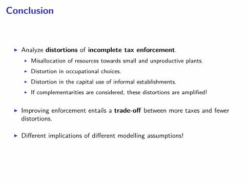
I Analyze distortions of incomplete tax enforcement.I Misallocation of resources towards small and unproductive plants.I Distortion in occupational choices.I Distortion in the capital use of informal establishments.I If complementarities are considered, these distortions are amplified!
I Improving enforcement entails a trade-off between more taxes and fewerdistortions.
I Different implications of different modelling assumptions!

Thank you!

Appendix
Aggregation
270 J.C. Leal Ordóñez / Review of Economic Dynamics 17 (2014) 262–286
Fig. 2. Characterization of occupational decisions. (For interpretation of the references to color in this figure, the reader is referred to the web version ofthis article.)
I focus on the steady-state (SS) equilibrium of this economy. As is standard, the first-order conditions of this problem inthe steady state imply that:
r = 1β
− (1 − δ). (9)
3.4. Market clearing
The market-clearing condition for the labor market will equate the aggregate labor demand from the two sectors to thelabor supply:
z!
z
I(z; wt, rt)lI (z; wt, rt)dG(z) +z!
z
F (z; wt, rt)lF (z; wt, rt)dG(z) =z!
z
W (z; wt, rt)dG(z), (10)
where W (z; wt , rt) = 1 − I(z; wt , rt) − F (z; wt , rt). Market clearing for the capital and good markets are, respectively:
z!
z
I(z; wt, rt)kI (z; wt, rt)dG(z) +z!
z
F (z; wt, rt)kF (z; wt, rt)dG(z) = Kt,
and
Ct + Kt+1 − (1 − δ)Kt =z!
z
I(z; wt, rt)yI (z; wt, rt)dG(z) +z!
z
F (z; wt, rt)yF (z; wt, rt)dG(z).
3.5. Equilibrium definition
An equilibrium for this economy is sequences {Ct , Kt+1, wt , rt} and {It(z), Ft(z)} ∀z ∈ [z, z], whereby taking factor prices{wt, rt}, policies parameters τy and b, and transfers {Tt}, the household solves its problem, firms maximize their profits ∀t ,and markets clear ∀t .
3.6. Steady state
In the following section, I will focus on the steady-state equilibrium. Since I define time-invariant taxation and enforce-ment policies, the dynamic part of this economy is no different from that in the standard growth model. In the steady state,factor prices, occupational decisions, aggregate capital and output are constant over time.
4. Properties of the model
4.1. Occupational choices
In this section, I analyze a number of properties of the model. The steady-state equilibrium is characterized by threethresholds, {z1, zc, z2}, which summarize the occupational decisions of the agents and whether the capital choices of infor-mal entrepreneurs are constrained or unconstrained. Fig. 2 provides a graph of the optimal occupational choices. I study thedetermination of these thresholds next.
EquilibriumAn equilibrium for this economy is sequences {Ct,Kt+1,wt, rt} and It(z), Ft(z)∀z ∈ [z, z], whereby taking factor prices {wt, rt}, policies parameters τy and b,and transfers {Tt}, the household solves its problem, firms maximize their profits∀t, and markets clear ∀t.
AppendixCALIBRATION
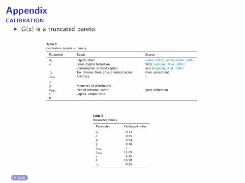
I G(z) is a truncated pareto.274 J.C. Leal Ordóñez / Review of Economic Dynamics 17 (2014) 262–286
Table 3Calibration targets summary.
Parameter Target Source
θk Capital share Gollin (2002), Garcia-Verdu (2005)δ Gross capital formation WDI, Solimano et al. (2005)
Consumption of fixed capital and Bergoeing et al. (2001)τy Tax revenue from private formal sector Own assessmentzmin Arbitrary –
γβ Moments of distributionzmax Size of informal sector Joint calibrations Capital–output ratiob
Table 4Calibration targets.
Targeted variables Data Model
K/Y 2.0 2.1Mean size 5.5 5.8Informal size 0.45 0.45Mean size by employment size category:More than 100 362 360Worker share by employment size category:More than 100 0.30 0.28
Fig. 5. Calibration properties: non-targeted moments.
parameter values that replicate the data fairly well, even in highly disaggregated size categories, despite the fact that I donot target such moments. I present a summary of the calibration targets in Table 3.
5.2. Calibration properties
The targeted moments are well matched as can be confirmed in Table 4, which presents data and model values.Perhaps more interesting is the fact that the calibration yields parameters that replicate well a number of moments that
were not targeted explicitly. In Fig. 5, the model is shown to replicate the mean size for a number of highly disaggregatedsize categories.
The calibrated parameter values are presented in Table 5. Note that the value of γ is 0.76, relatively low compared tothat found in studies focused on the United States. In particular, Atkeson and Kehoe (2005) estimate a value of 0.85 forUS manufactures. γ controls the returns to scale at the establishment level. The closer γ is to 1, the lower the degree of
J.C. Leal Ordóñez / Review of Economic Dynamics 17 (2014) 262–286 275
Table 5Parameter values.
Parameter Calibrated value
θk 0.33δ 0.05β 0.94γ 0.76zmin 1zmax 13.05s 4.25b 10.50τy 0.25
Table 6Short-run effects: First period after change in enforcement.
Variable Value under complete enforcementrelative to benchmark
Y 1.044τy 1K 1TFP 1.044L 1.120µ 2.104r 1.130w 0.829
decreasing returns and the more efficient it is to concentrate production in large establishments. In the limiting case ofγ = 1 (constant returns to scale), efficient output is reached by concentrating all resources in a single unit, i.e., the mostproductive one. The low value of γ I find implies that the distortion-free allocation for Mexico is to have more workers insmall units than would be the case in countries where the degree of decreasing returns is smaller (i.e., a larger γ ).
That the distortion-free allocation in Mexico is different than that in the US is not necessarily a bad result. It is not thethesis of this paper that the differences between Mexico and US distributions are due solely to tax enforcement differences.It could be argued that Mexico’s distortion-free skewed distribution is merely the result of its early stage of development.A number of authors have documented the steady rise in average firm size in the US during the 19th and 20th century (fora short bibliography, see Desmet and Parente, 2009). Furthermore, when one looks at the distribution of US of the past, at apoint in time during which the US had the same GDP per capita as modern-day Mexico (around the 1930s), it is clear thatit was not as highly concentrated in small establishments as it is in today’s Mexico.12
Finally, one more feature of the calibrated economy is that all informal entrepreneurs are constrained (i.e. that zc ≈ z1),which is roughly consistent with the evidence in Fig. 1.13
6. Results of the baseline model
Once the model is calibrated to the Mexican economy, I can investigate the effects of incomplete enforcement policies.To do this, I use this calibrated economy as a benchmark and perform three exercises: one that focuses on short-run effectsand two more that explore long-run effects. In these exercises, I introduce complete tax enforcement by making b = 0 inthe model; this implies that all establishments would pay a uniform tax (τy).
As a first step, I look at the equilibrium in the first period, immediately after the new enforcement policy is introduced.In this period, the capital stock is the same as in the economy with incomplete enforcement, because accumulation has notoccurred yet. Table 6 shows the value of aggregate variables in this context. Since capital and employment (employees +entrepreneurs) are no different from the benchmark economy, the only reason that output increases is that these resourcesare used more efficiently. Not surprisingly, output increases proportionally with TFP. Also, notice that in this first period,wages decrease.
The gains in TFP are associated with the removal of the distortions present under incomplete tax enforcement. The effectsof incomplete enforcement include distorting three margins: optimal occupational choices, allocation of resources acrossestablishments, and the capital–labor ratios of informal establishments. The first two distortions occur across establishments,while the last occurs within establishments. Incomplete tax enforcement distorts occupational choices because it makesentrepreneurship more attractive; furthermore it distorts the allocation of resources directly because it makes it possible tohave some establishments paying taxes and some others not; finally, it distorts the capital–labor ratio of a group of informalestablishments, because this is the optimal response to a probability of detection that increases with capital.
The short-run gains in TFP respond to the elimination of the distortions mentioned above. Note first, that the em-ployee/entrepreneur threshold z1 increases because a group of low-ability individuals no longer find it attractive to beentrepreneurs, so the average ability in the economy (µ in Table 6) improves14; second, note that since every establishmentpays the same tax rate, marginal products are equalized and the allocation of resources improves; and finally, note thatsince the probability of detection plays no important role under full enforcement, capital–labor ratios become undistorted.
In Table 6, it can be confirmed that, as a result of the change in threshold z1, the proportion of employees in theeconomy increases by 12% and the average ability by 110%. Note that consistent with this, wages decline to a level that is0.83 of the benchmark level. Also note that the rental rate of capital increases by 13% in this first period.
12 Granovetter (1984) documented the fact that the proportion of employees in US manufacturing establishments with fewer than 20 employees was 10%in 1933, while the proportion of employees in Mexican manufacturing establishments with fewer than 15 workers was 37.5% in 2005. Notice that the sizecategory is capped at a smaller size for Mexico than for the US, but the proportion allocated is still larger. Similarly, for the same size categories I find thatfor the retail and wholesale sectors, the figures are 63.8% and 44.4% for the US in 1939, and 72% and 48% for Mexico in 2005.13 This is clearer for construction, trade and services, which are the sectors where most of the informal entrepreneurs operate.14 This also entails a reduction in the mass of firms which reduces output, see Section 7 for a decomposition of the gains.
Back

AppendixCALIBRATION
274 J.C. Leal Ordóñez / Review of Economic Dynamics 17 (2014) 262–286
Table 3Calibration targets summary.
Parameter Target Source
θk Capital share Gollin (2002), Garcia-Verdu (2005)δ Gross capital formation WDI, Solimano et al. (2005)
Consumption of fixed capital and Bergoeing et al. (2001)τy Tax revenue from private formal sector Own assessmentzmin Arbitrary –
γβ Moments of distributionzmax Size of informal sector Joint calibrations Capital–output ratiob
Table 4Calibration targets.
Targeted variables Data Model
K/Y 2.0 2.1Mean size 5.5 5.8Informal size 0.45 0.45Mean size by employment size category:More than 100 362 360Worker share by employment size category:More than 100 0.30 0.28
Fig. 5. Calibration properties: non-targeted moments.
parameter values that replicate the data fairly well, even in highly disaggregated size categories, despite the fact that I donot target such moments. I present a summary of the calibration targets in Table 3.
5.2. Calibration properties
The targeted moments are well matched as can be confirmed in Table 4, which presents data and model values.Perhaps more interesting is the fact that the calibration yields parameters that replicate well a number of moments that
were not targeted explicitly. In Fig. 5, the model is shown to replicate the mean size for a number of highly disaggregatedsize categories.
The calibrated parameter values are presented in Table 5. Note that the value of γ is 0.76, relatively low compared tothat found in studies focused on the United States. In particular, Atkeson and Kehoe (2005) estimate a value of 0.85 forUS manufactures. γ controls the returns to scale at the establishment level. The closer γ is to 1, the lower the degree of
Back

AppendixMisallocation
278 J.C. Leal Ordóñez / Review of Economic Dynamics 17 (2014) 262–286
Table 9Pure misallocation effects.
Var. Bench. Full enforcement
Y 1 1.023TFP 1 1.023w 1 0.910r 1 1.107
slope in panel (c) around b = 1 is flatter than the slope around b = 0.5; thus, improvements in enforcement around thebenchmark create relatively small reductions in the informal sector.
One important lesson from Fig. 7 is that making enforcement worse also increases output. This occurs as marginal firms(near z1) enjoy a lower tax burden, while the burden on formal firms stays constant. This is consistent with the commonnotion that the informal sector is good for the economy as it allows firms to operate more efficiently. Fig. 7 helps us to seethe effects of increasing informality as a tradeoff: on the one hand, there is a positive force that originates from “lower”taxes; on the other, there is negative force that stems from resource misallocation, and from distorted occupational andcapital choices. When informality is high, the positive force dominates, because as informality increases, taxes are lower fora set of large and very productive establishments; in contrast, when informality is low, increasing informality reduces taxesfor a set of relatively small, and low-productive establishments. For middle levels of informality, these two forces tend tooffset each other and a U-shape relationship between informality and output emerges. In fact, Mexico, with an informalsector size equal to 45%, is close to the worst possible output level, which is associated with 35% informality.
7. Decomposing the gains from full enforcement
To decompose the gains from full tax enforcement, I perform a number of quantitative exercises asking what wouldhappen to the gains of eliminating distortions if I shut down or add specific features to the model. I start by analyzing astatic endowment economy version of the model and then take out or add features, following the guidelines of five leadingpapers in the literature on resource misallocation across plants. I classify these papers into three groups: (a) Restucciaand Rogerson (2008), which assumes free entry to determine the mass of firms in equilibrium; (b) Gollin (1995) andGuner et al. (2008), which emphasize occupational choices; and (c) Hsieh and Klenow (2007) and Jones (2011), whichfocus on linkages and complementarities using models with monopolistic competition. The contribution of this exercise istwofold: first, it provides a way to decompose the gains from full enforcement; second, it clarifies the differences amongthe aforementioned papers by comparing the results that alternative models provide for the same change in policy.
7.1. Marginal product equalization
As a first step, I look at the effects of full enforcement in a static endowment economy version of the model where thesupply of labor, the supply of capital, the mass of firms, and the average ability of entrepreneurs are all fixed. The resultsare presented in Table 9.
The economy in Table 9 operates with exactly the same resources as the benchmark economy. Since all resources arefixed, the only way to increase output is through a better allocation of resources. With the introduction of full enforce-ment, marginal products are equalized across establishments; therefore, this exercise isolates the pure effect of resourcemisallocation across plants.
Notice also that the introduction of full enforcement has an asymmetric impact on factor returns: wages go down, butthe rental rate of capital increases. This is intuitive: on the one hand, higher taxes affect both factor prices; on the other,the elimination of capital constraints increases both the demand for capital and r.
Since marginal products are equalized under full enforcement, this leads to an important issue regarding the decompo-sition of output gains. When there is no informal sector and marginal products are equalized, we can express aggregateoutput as a function of four main aggregates15:
Y = N1−γ µ1−γ K θk Lθl , (17)
where K is aggregate capital, L is aggregate labor (employees), N is the mass of firms, and µ is average entrepreneurialability. Given the 2.3% gain from a better allocation of resources, the remaining gains associated with full enforcement mustbe generated by changes in the amount of the productive factors in Eq. (17).
15 See Appendix B.
Back

Free entry
I Value of entry
We =
∫ zz1
π(z)g(z|z > z1)
1−G(z1) dz− ce
I Mass of entry computed as
G(z1)︸ ︷︷ ︸L
= N
∫ zz1
l(z)g(z|z > z1)
1−G(z1) dz
J.C. Leal Ordóñez / Review of Economic Dynamics 17 (2014) 262–286 279
Table 10Effects on factor levels.
Var. Bench. A. Free entry Occupational choices
B. Short run C. Long run
Y 1 0.925 1.044 1.109K 1 1 1 1.200L 1 1 1.120 1.120N 1 0.662 0.424 0.424µ 1 1 2.104 2.104TFP 1 0.925 1.044 1.044
Table 11Decomposing gains of perfect enforcement.
Var. A = MP equalization B = A + free entry C = A + occupational choice D = C + capital accumulation Total
Y 1.02 0.92 1.04 1.11(△Y ) +2 −10 +12 +7 +11TFP 1.02 0.91 1.04 1.04△TFP +2 −10 +12 0 +4
7.2. The mass of firms (adding free entry)
To investigate the importance of distortions in the mass of firms, I add a free-entry condition but keep the assumptions ofa fixed endowment of labor, a fixed endowment of capital, and a fixed average ability (i.e., I shut down occupational choicesand investments). This modification brings the model closer that used by Restuccia and Rogerson (2008) (group “a”).
Consider a potential entrepreneur that is evaluating whether to enter or not. This agent takes into account the expectedprofits of incumbent entrepreneurs. Thus, the value of entry is described by:
We =z!
z1
π(z)g(z)dz − ce,
where g(z) = g(z|z > z1)/(1 − G(z1)), ce is an entry cost, π(z) are profits, and z1 is given by w = πM(z1; w, r) (from thebenchmark, in the baseline model). Now let N be the mass of firms and E the endowment of labor; the labor marketclearing condition is as follows:
E = N
z!
z1
l(z)g(z)dz,
where E = 1 − G(z1).Notice that in this economy, average entrepreneurial ability is constant, independent of N , and is equal to µ =
" zz1
z1
1−γ g(z)dz. Given ce , I can find equilibrium allocations by solving the free entry and the labor market clearing con-
ditions for w and N . Column A in Table 10 shows the results.16
The introduction of complete enforcement reduces We because the expected value of incumbent entrepreneurs is hit byhigher taxes; therefore, the mass of firms is negatively affected. In Eq. (17), the mass of firms is an important component ofaggregate output, thus output decreases. We can perform the accounting of output losses using Eq. (17). Letting Y1 be thevalue of output in Table 9 and Y the corresponding value in Table 10, the effect of full enforcement under this exercise is:YY1
= 0.6620.24 ≈ 0.9251.023 ≈ 0.904. Thus, adding firm entry reduces output by 10% (see also Table 11).
7.3. Occupational choices
Now consider an economy with an occupational-choice rather than a free-entry condition, but keep the assumption of afixed capital stock. This brings the model closer to Gollin (1995) and Guner et al. (2008) (group “b”), and is also our baselinemodel in the short run. Adding occupational choices will bring good news, because it will allow the economy to increaseaverage ability and the supply of labor, while reducing entry.
Notice first that the introduction of full enforcement pushes z1 to the right. As a result, the mass of firms N = 1 − G(z1)is reduced; however, the average ability µ and the supply of labor F (z1) both increase. This exercise is identical to that
16 To obtain the value of ce , I use the fact that We must be zero in equilibrium (the free-entry condition) and set it equal to the value of" z
z1π(z)g(z)dz
in the benchmark.
Back

Monopolistic competition - Set upI Final good producer aggregates intermediates with CRS technology.
Y =
(∫y(w)ρdω
)ρI Demand for each variety is
y(ω) =
(p(ω)
P
)−σ(I
P
)(6)
whereI Price index: P =
(∫p(w)1−σdω
)1/rhoI Aggregate demand of intermediates: I =
∫p(ω)y(ω)dω.
I Intermediate good producers have a Cobb-Douglas technology
y(x) = xkαl1−α (7)
I Maximizep(x)y(x) −wl(x) − rk(x) s.t. (6) and (7).
Back

Monopolistic competition - Set up
Equivalence between perfect and monopolistic competition.I If the following conditions are met, the equilibrium allocations between the
two models are exactly the same.
J.C. Leal Ordóñez / Review of Economic Dynamics 17 (2014) 262–286 281
p(x)y(x) − wl(x) − rk(x),
therefore, the problem for a producer x is to maximize profits subject to Eqs. (18) and (19).
8.3. Household problem
I keep the feature of the model that includes a representative household populated by a continuum of members withabilities x and each member faces an occupational choice, as in the benchmark model. The household problem with mo-nopolistic competition is only slightly different from that in the model with perfect competition, with one difference beingin the budget constraint. In the case of monopolistic competition, we have a firm that produces the final good—which isowned by the household—and its profits must be part of the resources available to the household. It is found that, due toCRS, the profits for the final producer are zero in equilibrium.
A further difference is in the profits of the intermediate producers x ∈ (x, x), which are, in general, different from theprofits of entrepreneurs z ∈ (z, z). However, by choosing the right value of the parameters, an equivalence between thesetwo models can be established.
8.4. Equivalency between perfect- and monopolistic-competition models
Equilibrium allocations in the model with perfect competition can be delivered by the model with monopolistic compe-tition, provided certain conditions are placed on the parameters and the productivity levels. To demonstrate this, first letus note the following equivalency between establishment z’s problem in the model with perfect competition and that forproducer x in the model with monopolistic competition. Producer x’s sales are:
p(x)y(x) = I(1/σ ) y(x)σ−1σ = I(1/σ )x
σ−1σ kα σ−1
σ l(1−α) σ−1σ , (20)
where the first equality arrives when using Eq. (18) to substitute for p(x) and the second when we use Eq. (19) to substitutefor y(x). Conversely, remember that sales for a typical establishment z in the perfect-competition model are simply givenby y(z) = zkθk lθl . Furthermore, notice that the total cost in both problems is (wl + rk) and, therefore, the optimal choices ofentrepreneur z in the perfect-competition model will be the same as the optimal choices of the intermediate producer x inthe model with imperfect competition, provided the following conditions are met18:
1.
z = I(1/σ )xσ−1σ , ∀z ∈ (z, z),
2.
θk = ασ − 1
σ, and
3.
θl = (1 − α)σ − 1
σ.
If the above three conditions hold, then the equilibrium allocations are exactly the same in both models. Moreover, givenequilibrium allocations for the perfect-competition model, we can always choose values of α, σ , and x ∈ (x, x), such thatthe above conditions hold. This equivalency is satisfied regardless of whether we are dealing with the incomplete or thecomplete enforcement versions. I use the aforementioned conditions to obtain α, σ , and x ∈ (x, x), such that the twoproblems referred to above are equivalent. I compute this equivalency for the incomplete enforcement versions.
8.5. Full enforcement with monopolistic competition
Now, I introduce complete enforcement in the model with monopolistic competition and look at the new steady state.Table 12 shows the results. Adding monopolistic competition triples the gains in measured TFP, increases capital accumula-tion by a factor of 1.33, and output by a factor of 1.8 with respect to perfect competition. The gains in TFP and output arenot negligible. Restuccia (2008) studies the Latin American development problem and finds that in a model with human-capital accumulation, TFP would have to increase 60% in order to eliminate the gap in income per capita between thesecountries and the US. Thus, introducing full enforcement could make a 20% (12/60) contribution to achieving this goal.
The mechanics of the multiplier are evident in condition 1 above. Notice that the productivity of each firm is nowaffected by aggregate demand (I). Since a distortion in one firm affects aggregate demand, it also affects the productivity ofthe remaining firms, which in turn feeds back into I , and so on.
18 This point is also found in footnote 6 in Restuccia and Rogerson (2008).
Back

Monopolistic competition - Decomposition282 J.C. Leal Ordóñez / Review of Economic Dynamics 17 (2014) 262–286
Table 12Complete enforcement with monopolistic competition.
Perfect competition Monopolistic competition
Fixed tax rate Revenue neutral Fixed tax rate Revenue neutral
Y 1.11 1.19 1.18 1.34K 1.20 1.50 1.27 1.70TFP 1.04 1.04 1.09 1.12
Table 13Summary of output-loss decomposition (%).
Discontinuous dist. Continuous dist. Relative Related paper
Total loss with fixed revenue −0.34 −0.24 0.70Total loss with fixed tax rate −0.18 −0.12 0.66Contribution of
factor misallocation 0.13 0.11 0.57firm entry −0.56 −0.39 0.46 RRoccupational choices 0.68 0.47 0.45 Gollin, GVXcapital accumulation 0.37 0.43 0.77complementarities 0.38 0.37 0.65 HK, Jones
9. Summary of the output-loss decomposition
Table 13 presents a summary of the decomposition of output losses. It presents this decomposition for both the discon-tinuous distortion analyzed here and a continuous distortion analyzed in Appendix C (see also Section 9.1). For the case ofthe step function (discontinuous distortion), the total loss is 18% when the tax rate is fixed; this, in turn, can be decomposedinto five sources: factor misallocation, firm entry, distortions of occupational choices, capital accumulation, and complemen-tarities. Pure factor misallocation contributes 13% to the output loss, firm entry −56%, occupational choices 68%, capitalaccumulation 37%, and complementarities 38%. Notice that informality has a positive effect on output because it providesan incentive to firm entry, so the increase in the mass of firms contributes −56% to the output loss. This is reversed by thecontribution of occupational choices, which increase average ability and labor supply, whilst reducing entry. Thus, the netcontribution of occupational choices and free entry is 12% (68–56%).
9.1. Discussion
A natural question that arises from this analysis is, what is the cost of increasing enforcement? These costs have to besubtracted from the output gains reported in the previous section, in order to provide a sense of the net gain associatedwith the policy change in question.
Since the informal sector consists of many small businesses, better enforcement increases the number of taxpayers overwhich the authorities need to provide surveillance. In the benchmark, there are 22 times more informal establishmentsthan formal establishments; in other words, informal establishments represent 95% of all entrepreneurs. According to offi-cial Mexican tax authority data, the office currently spends around 1 peso for every 100 pesos collected.19 We can use thisinformation to obtain the enforcement cost per establishment in the model and then calculate the cost of full enforcement,assuming that cost per establishment is a constant and taking into account the increase in the number of formal establish-ments. I calculate that introducing full enforcement will increase total enforcement costs by a factor of 9.6, a huge increase;however, it represents a small fraction of gross revenue. Gross revenue increases to 25% of the model’s GDP and enforce-ment costs to 1.3% of GDP. This means that most of the gains in enforcement remain after subtracting the extra monitoringcosts.
Another source of concern is the importance of the assumption regarding the shape of the probability of detection.So far I have assumed that this probability has a discontinuity. In Appendix C, I investigate the sensitivity of my resultsto this assumption; I find that the bulk of the output losses driven by incomplete enforcement remain when a continuousdistortion is considered. In particular, I use a linear function and find that output losses would be 75% of the losses in thebaseline case.
In Table 13, the decomposition of output losses is also presented for the continuous distortion case. Notice that thebulk of the effects remain when a continuous distortion is considered. However, not all sources of distortions remain withthe same intensity. For example, capital accumulation and complementarities remain as important as in the discontinuousdistortion case, whilst factor misallocation and distortions of occupational choices, as well as firm entry seem less important.
19 This information is available at http://www.sat.gob.mx/sitio_internet/transparencia/51_8833.html.
Back