HAL Id: tel-01386600https://tel.archives-ouvertes.fr/tel-01386600

Submitted on 24 Oct 2016

HAL is a multi-disciplinary open accessarchive for the deposit and dissemination of sci-entific research documents, whether they are pub-lished or not. The documents may come fromteaching and research institutions in France orabroad, or from public or private research centers.

L’archive ouverte pluridisciplinaire HAL, estdestinée au dépôt et à la diffusion de documentsscientifiques de niveau recherche, publiés ou non,émanant des établissements d’enseignement et derecherche français ou étrangers, des laboratoirespublics ou privés.

Task-based multifrontal QR solver for heterogeneousarchitectures

Florent Lopez

To cite this version:Florent Lopez. Task-based multifrontal QR solver for heterogeneous architectures. Distributed, Par-allel, and Cluster Computing [cs.DC]. Université Paul Sabatier - Toulouse III, 2015. English. <NNT :2015TOU30303>. <tel-01386600>

THESEEn vue de l’obtention du

DOCTORAT DE L’UNIVERSITE DE TOULOUSE

Délivré par :

L’Université Paul Sabatier

Présentée et soutenue par :

Florent Lopez

Le 11 décembre 2015

Titre :

Task-based multifrontal QR solver for heterogeneous architectures

Solveur multifrontal QR à base de tâches pour architectures hétérogènes

Ecole doctorale et discipline ou spécialité :

ED MITT : Domaine STIC : Sûreté du logiciel et calcul haute performance

Unité de recherche :

IRIT - UMR 5505

Directeurs de Thèse :

Michel Daydé (ENSEEIHT-IRIT)Alfredo Buttari (CNRS-IRIT)

Rapporteurs :

Timothy A. Davis (Texas A&M University)Pierre Manneback (Universite de Mons)

Autres membres du jury :

Frédéric Desprez (Inria Rhône-Alpes)Iain S. Duff (Rutherford Appleton Laboratory)Raymond Namyst (Inria Bordeaux Sud-Ouest)

Résumé

Afin de s’adapter aux architectures multicoeurs et aux machines de plus en plus complexes,les modèles de programmations basés sur un parallélisme de tâche ont gagné en popularitédans la communauté du calcul scientifique haute performance. Les moteurs d’exécutionfournissent une interface de programmation qui correspond à ce paradigme ainsi que desoutils pour l’ordonnancement des tâches qui définissent l’application.

Dans cette étude, nous explorons la conception de solveurs directes creux à base detâches, qui représentent une charge de travail extrêmement irrégulière, avec des tâches degranularités et de caractéristiques différentes ainsi qu’une consommation mémoire variable,au-dessus d’un moteur d’exécution. Dans le cadre du solveur qr mumps, nous montronsdans un premier temps la viabilité et l’efficacité de notre approche avec l’implémenta-tion d’une méthode multifrontale pour la factorisation de matrices creuses, en se basantsur le modèle de programmation parallèle appelé “flux de tâches séquentielles” (SequentialTask Flow). Cette approche, nous a ensuite permis de développer des fonctionnalités tellesque l’intégration de noyaux dense de factorisation de type “minimisation de communica-tions” (Communication Avoiding) dans la méthode multifrontale, permettant d’améliorerconsidérablement la scalabilité du solveur par rapport a l’approche original utilisée dansqr mumps. Nous introduisons également un algorithme d’ordonnancement sous contraintesmémoire au sein de notre solveur, exploitable dans le cas des architectures multicoeur, ré-duisant largement la consommation mémoire de la méthode multifrontale QR avec unimpacte négligeable sur les performances.

En utilisant le modèle présenté ci-dessus, nous visons ensuite l’exploitation des archi-tectures hétérogènes pour lesquelles la granularité des tâches ainsi les stratégies l’ordon-nancement sont cruciales pour profiter de la puissance de ces architectures. Nous pro-posons, dans le cadre de la méthode multifrontale, un partitionnement hiérarchique desdonnées ainsi qu’un algorithme d’ordonnancement capable d’exploiter l’hétérogénéité desressources. Enfin, nous présentons une étude sur la reproductibilité de l’exécution parallèlede notre problème et nous montrons également l’utilisation d’un modèle de programmationalternatif pour l’implémentation de la méthode multifrontale.

L’ensemble des résultats expérimentaux présentés dans cette étude sont évalués avecune analyse détaillée des performance que nous proposons au début de cette étude. Cetteanalyse de performance permet de mesurer l’impacte de plusieurs effets identifiés sur lascalabilité et la performance de nos algorithmes et nous aide ainsi à comprendre pleinementles résultats obtenu lors des tests effectués avec notre solveur.

Mots-clés : méthodes directes de résolution de systèmes linéaires, méthode multifron-tale, multicoeur, moteurs d’exécutions, ordonnancement, algorithmes d’ordonnancementsous contraintes mémoire, architectures hétérogènes, calcul haute performance, GPU

iii

Abstract

To face the advent of multicore processors and the ever increasing complexity of hardwarearchitectures, programming models based on DAG parallelism regained popularity in thehigh performance, scientific computing community. Modern runtime systems offer a pro-gramming interface that complies with this paradigm and powerful engines for schedulingthe tasks into which the application is decomposed. These tools have already proved theireffectiveness on a number of dense linear algebra applications.

In this study we investigate the design of task-based sparse direct solvers which con-stitute extremely irregular workloads, with tasks of different granularities and character-istics with variable memory consumption on top of runtime systems. In the context ofthe qr mumps solver, we prove the usability and effectiveness of our approach with theimplementation of a sparse matrix multifrontal factorization based on a Sequential TaskFlow parallel programming model. Using this programming model, we developed featuressuch as the integration of dense 2D Communication Avoiding algorithms in the multi-frontal method allowing for better scalability compared to the original approach used inqr mumps. In addition we introduced a memory-aware algorithm to control the memorybehaviour of our solver and show, in the context of multicore architectures, an impor-tant reduction of the memory footprint for the multifrontal QR factorization with a smallimpact on performance.

Following this approach, we move to heterogeneous architectures where task granu-larity and scheduling strategies are critical to achieve performance. We present, for themultifrontal method, a hierarchical strategy for data partitioning and a scheduling algo-rithm capable of handling the heterogeneity of resources. Finally we present a study onthe reproducibility of executions and the use of alternative programming models for theimplementation of the multifrontal method.

All the experimental results presented in this study are evaluated with a detailedperformance analysis measuring the impact of several identified effects on the performanceand scalability. Thanks to this original analysis, presented in the first part of this study,we are capable of fully understanding the results obtained with our solver.

Keywords: sparse direct solvers, multifrontal method, multicores, runtime systems,scheduling, memory-aware algorithms, heterogeneous architectures, high-performance com-puting, GPU

v

Acknowledgements

I am extremely grateful to Alfredo Buttari for his excellent supervision and constantsupport throughout three years of intensive work. Without his efforts this thesis wouldnot have been possible. Thanks also to my two co-advisors Emmanuel Agullo and AbdouGermouche for their fruitful collaborations and very interesting discussions. I also wish tothank Michel Daydé for his support during this thesis.

Thanks to Jack Dongarra and George Bosilca for their warm welcome at the Univer-sity of Tennessee, Knoxville, during my six month scholar visit to the ICL Laboratory.Thanks to the Distributed Computing team for the great collaboration, valuable help andintroducing me to the PaRSEC library.

I would like to thank all the members of the thesis committee for reviewing my dis-sertation and particularly the “Rapporteurs” Tim Davis and Pierre Manneback for theinsightful reports they provided about this manuscript. Also a big thank you to Iain Dufffor providing such a complete and detailed feedback on the dissertation.

Thanks to my colleagues and particularly my office mates who are now among myclosest friends: Francois-Henry Rouet, Clement Weisbecker, Mohamed Zenadi, ClementRoyet and Theo Mary. Thanks to them for the good moments we shared, and the adviceand support I received from you.

Finally, I’m deeply grateful to my family for their love, support and encouragementduring the production of this thesis.

vii

Contents

Résumé iii

Abstract v

Acknowledgements vii

1 Introduction 1

1.1 Architectures . . . . . . . . . . . . . . . . . . . . . . . . . . . . . . . . . . 11.2 Linear systems and direct methods . . . . . . . . . . . . . . . . . . . . . . 4

1.2.1 Problems/applications . . . . . . . . . . . . . . . . . . . . . . . . . 41.2.2 QR decomposition . . . . . . . . . . . . . . . . . . . . . . . . . . . 61.2.3 Multifrontal QR methods . . . . . . . . . . . . . . . . . . . . . . . 9

1.3 Parallelization of the QR factorization . . . . . . . . . . . . . . . . . . . . 141.3.1 Dense QR factorization . . . . . . . . . . . . . . . . . . . . . . . . 141.3.2 Sparse QR factorization . . . . . . . . . . . . . . . . . . . . . . . . 17

1.4 Programming models and runtime systems . . . . . . . . . . . . . . . . . . 171.4.1 Programming models for task-based applications . . . . . . . . . . 181.4.2 Task-based runtime systems for modern architectures . . . . . . . 20

1.4.2.1 The StarPU runtime system . . . . . . . . . . . . . . . . 221.4.2.2 The PaRSEC runtime system . . . . . . . . . . . . . . . . 25

1.5 Related work on dense linear algebra . . . . . . . . . . . . . . . . . . . . . 271.6 Related work on sparse direct solvers . . . . . . . . . . . . . . . . . . . . . 281.7 The qr mumps solver . . . . . . . . . . . . . . . . . . . . . . . . . . . . . . 30

1.7.1 Fine-grained parallelism in qr mumps . . . . . . . . . . . . . . . . . 301.7.2 Tree pruning . . . . . . . . . . . . . . . . . . . . . . . . . . . . . . 341.7.3 Blocking of dense matrix operations . . . . . . . . . . . . . . . . . 351.7.4 The qr mumps scheduler . . . . . . . . . . . . . . . . . . . . . . . . 36

1.7.4.1 Scheduling policy . . . . . . . . . . . . . . . . . . . . . . 361.8 Positioning of the thesis . . . . . . . . . . . . . . . . . . . . . . . . . . . . 381.9 Experimental settings . . . . . . . . . . . . . . . . . . . . . . . . . . . . . 40

1.9.1 Machines . . . . . . . . . . . . . . . . . . . . . . . . . . . . . . . . 401.9.2 Problems . . . . . . . . . . . . . . . . . . . . . . . . . . . . . . . . 41

2 Performance analysis approach 45

2.1 General analysis . . . . . . . . . . . . . . . . . . . . . . . . . . . . . . . . 462.2 Discussion . . . . . . . . . . . . . . . . . . . . . . . . . . . . . . . . . . . . 50

3 Task-based multifrontal method: porting on a general purpose runtimesystem 53

3.1 Efficiency and scalability of the qr mumps scheduler . . . . . . . . . . . . . 53

ix

Contents

3.2 StarPU-based multifrontal method . . . . . . . . . . . . . . . . . . . . . . 543.2.1 DAG construction in the runtime system . . . . . . . . . . . . . . 543.2.2 Dynamic task scheduling and memory consumption . . . . . . . . 583.2.3 Experimental results . . . . . . . . . . . . . . . . . . . . . . . . . . 60

4 STF-parallel multifrontal QR method on multicore architecture 654.1 STF-parallel multifrontal QR method . . . . . . . . . . . . . . . . . . . . 65

4.1.1 STF-parallelization . . . . . . . . . . . . . . . . . . . . . . . . . . . 654.2 STF multifrontal QR method 1D . . . . . . . . . . . . . . . . . . . . . . . 69

4.2.1 STF parallelization with block-column partitioning . . . . . . . . . 694.2.2 Experimental results . . . . . . . . . . . . . . . . . . . . . . . . . . 714.2.3 The effect of inter-level parallelism . . . . . . . . . . . . . . . . . . 75

4.3 STF multifrontal QR method 2D . . . . . . . . . . . . . . . . . . . . . . . 764.3.1 Experimental results . . . . . . . . . . . . . . . . . . . . . . . . . . 794.3.2 Inter-level parallelism in 1D vs 2D algorithms . . . . . . . . . . . . 83

4.4 Task scheduling with lws . . . . . . . . . . . . . . . . . . . . . . . . . . . 85

5 Memory-aware multifrontal method 895.1 Memory behavior of the multifrontal method . . . . . . . . . . . . . . . . 895.2 Task scheduling under memory constraint . . . . . . . . . . . . . . . . . . 91

5.2.1 The sequential case . . . . . . . . . . . . . . . . . . . . . . . . . . . 915.2.2 The parallel case . . . . . . . . . . . . . . . . . . . . . . . . . . . . 92

5.3 STF Memory-aware multifrontal method . . . . . . . . . . . . . . . . . . . 935.4 Experimental results . . . . . . . . . . . . . . . . . . . . . . . . . . . . . . 95

6 STF-parallel multifronatal QR method on heterogeneous architecture 996.1 Frontal matrices partitioning schemes . . . . . . . . . . . . . . . . . . . . 996.2 Scheduling strategies . . . . . . . . . . . . . . . . . . . . . . . . . . . . . . 1026.3 Implementation details . . . . . . . . . . . . . . . . . . . . . . . . . . . . . 1056.4 Experimental results . . . . . . . . . . . . . . . . . . . . . . . . . . . . . . 106

6.4.1 Performance and analysis . . . . . . . . . . . . . . . . . . . . . . . 1066.4.2 Multi-streaming . . . . . . . . . . . . . . . . . . . . . . . . . . . . 1106.4.3 Comparison with a state-of-the-art GPU solver . . . . . . . . . . . 112

6.5 Possible minor, technical improvements . . . . . . . . . . . . . . . . . . . 113

7 Associated work 1157.1 PTG multifrontal QR method . . . . . . . . . . . . . . . . . . . . . . . . . 1157.2 Simulation of qrm starpu with StarPU SimGrid . . . . . . . . . . . . . . 1207.3 StarPU contexts in qrm starpu . . . . . . . . . . . . . . . . . . . . . . . . 124

8 Conclusion 1298.1 General conclusion . . . . . . . . . . . . . . . . . . . . . . . . . . . . . . . 1298.2 Perspectives and future work . . . . . . . . . . . . . . . . . . . . . . . . . 130

Submitted articles . . . . . . . . . . . . . . . . . . . . . . . . . . . . . . . 133Conference proceedings . . . . . . . . . . . . . . . . . . . . . . . . . . . . 133Posters . . . . . . . . . . . . . . . . . . . . . . . . . . . . . . . . . . . . . . 133Conference talks . . . . . . . . . . . . . . . . . . . . . . . . . . . . . . . . 133

References 135

x

Chapter 1

Introduction

1.1 Architectures

The world of computing, and particularly the world of High Performance Computing(HPC), have witnessed a substantial change at the beginning of the last decade as all theclassic techniques used to improve the performance of microprocessors reached the point ofdiminishing returns [17]. These techniques, such as deep pipelining, speculative executionor superscalar execution, were mostly based on the use of Instruction Level Parallelism(ILP) and required higher and higher clock frequencies to the point where the processorspower consumption, which grows as the cube of the clock frequency, became (or wasabout to become) unsustainable. This was not only true for large data or supercomputingcenters but also, and even more so, for portable devices such as laptops, tablets andsmartphones which have recently become very widespread. In order to address this issue,the microprocessor industry sharply turned towards a new design based on the use ofThread Level Parallelism (TLP) achieved by accommodating multiple processing units orcores on the same die. This led to the production of multicore processors that are nowadaysubiquitous. The main advantage over the previous design principles lies in the fact thatthe multicore design does not require an increase in the clock frequency but only impliesan augmentation of the chip capacitance (i.e., the number of transistors) on which thepower consumption only depends linearly. As a result, the multicore technology not onlyenables improvement in performance, but also reduces the power consumption: assuminga single-core processor with frequency f , a dual-core with frequency 0.75 ∗ f is 50% fasterand consumes 15% less energy.

Since their introduction, multicore processors have become increasingly popular andcan be found, nowadays, in almost any device that requires some computing power. Be-cause they allow for running multiple processes simultaneously, the introduction of multi-core in high throughput computing or in desktop computing was transparent and imme-diately beneficial. In HPC, though, the switch to the multicore technology lead to a sharpdiscontinuity with the past as methods and algorithms had to be rethought and codesrewritten in order to take advantage of the added computing power through the use ofTLP. Nonetheless, multicore processors have quickly become dominant and are currentlyused in basically all supercomputers. Figure 1.1 (left) shows the performance share of mul-ticore processors in the Top5001 list (a list of the 500 most powerful supercomputers in theworld, which is updated twice per year); the figure shows that after their first appearancein the list (May 2005) multicore has quickly become the predominant technology in theTop500 list and ramped up to nearly 100% of the share in only 5 years. The figure also

1http://top500.org

1

1. Introduction

0

20

40

60

80

100

93 95 97 99 01 03 05 07 09 11 13 15

Year

Cores per socket -- performance share

60

32

18

14

10

12

8

16

6

9

4

2

1

0

20

40

60

80

100

93 95 97 99 01 03 05 07 09 11 13 15

Year

Accelerators -- performance share

PEZY-SC

Hybrid

Nvidia Kepler

Intel Xeon Phi

ATI Radeon

Nvidia Fermi

IBM Cell

Clearspeed

None

Figure 1.1: Performance share of multicore processors (on the left) and accelerators (onthe right) in the Top500 list.

shows that the number of cores per socket has grown steadily over the years: a typicalmodern processor features between 8 and 16 cores. In Section 1.9.1 we present the sys-tems used for the experiments reported in this document. The most recent and powerfulamong these processors is the Xeon E5-2680 which hosts 12 cores; each of these cores has256 bit AVX vector units with Fused Multiply-Add (FMA) capability which, with a clockfrequency of 2.5 GHz make a peak performance of 40 Gflop/s per core and 480 Gflop/son the whole processor for double-precision floating point operations.

Around the same period as the introduction of multicore processors, the use of ac-celerators or coprocessors started gaining the interest of the HPC community. Althoughthis idea was not new (for example FPGA boards were previously used as coprocessors),it was revamped thanks to the possibility of using extremely efficient commodity hard-ware for accelerating scientific applications. One such example is the Cell processor [65]produced by the STI consortium (formed by IBM, Toshiba and Sony) from 2005 to 2009.The Cell was used as an accelerator board on the Roadrunner supercomputer installedat the Los Alamos National Labrador (USA) which was ranked #1 in the Top500 list ofNovember 2008. The use of accelerators for HPC scientific computing, however, gained avery widespread popularity with the advent of General Purpose GPU computing. Specif-ically designed for image processing operations, Graphical Processing Units (GPUs) offera massive computing power which is easily accessible for highly data parallel applications(image processing often consists in repeating the same operation on a large number ofpixels). This led researchers to think that these devices could be employed to acceleratescientific computing applications, especially those based on the use of operations with avery regular behaviour and data access pattern, such as dense linear algebra. In the lastfew years, GPGPU has become extremely popular in scientific computing and is employedin a very wide range of applications, not only dense linear algebra. This widespread useof GPU accelerators was also eased by the fact that GPUs, which were very limited incomputing capabilities and difficult to program, have become, over the years, suited toa much wider range of applications and much easier to program thanks to the devel-

2

1.1. Architectures

opment of specific high-level programming languages and development kits. Figure 1.1(right) shows the performance share of supercomputers equipped with accelerators. Al-though some GPU accelerators are also produced by AMD, currently the most widelyused ones are produced by Nvidia. Figure 1.2 shows a block diagram of the architectureof a recent Nvidia GPU device, the K40m of the Kepler family. This board is equippedwith 15 Streaming Multiprocessors (SMX), each containing 192 single precision cores and64 double precision ones for a peak performance of 1.43 (4.29) Tflop/s for double (single)precision computations. The K40m also has a memory of 12 GB capable of streaming dataat a speed of 288 GB/s.

More recently Intel has also started producing accelerators, namely the Xeon Phiboards. The currently distributed models of the Xeon Phi devices, the Knights Cornerfamily, can host up to 61 cores connected with a bi-directional ring interconnect. Eachcore has a 512 bit wide vector unit with FMA capability and the clock frequency canbe as high as 1.238 GHz which makes an overall maximum peak performance of 1208Gflop/s for double-precision, floating point computation. On-board memory can be as bigas 16 GB and transfer data at a speed of 352 GB/s. One outstanding advantage of theXeon Phi devices is that the instruction set is fully x86 compliant which allows for using“traditional” multithreading programming technologies such as OpenMP.

Figure 1.2: Block diagram of the Kepler K40m GPU.

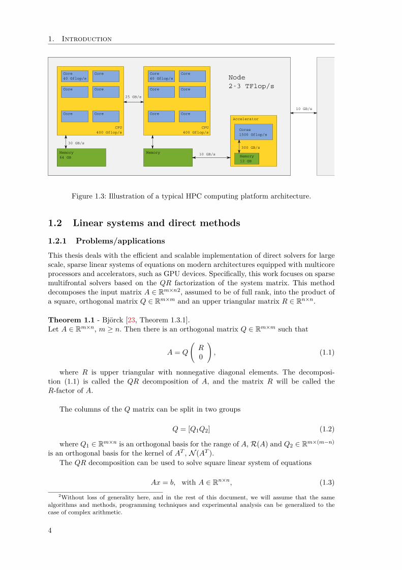
Figure 1.3 shows a typical configuration of a modern HPC computing platform. This isformed by multiple (up to thousands) nodes connected through a high-speed network; eachnode may include multiple processors, each connected with a NUMA memory module. Anode may also be equipped with one or more accelerators. Please note that the figurereports indicative values for performance, bandwidths and memory capacities and do notrefer to any specific device. The figure shows that modern HPC platforms are basedon extremely heterogeneous architectures as they employ processing units with differentperformance, memories with different capacities and interconnects with different latenciesand bandwidths.

3

1. Introduction

Core40 Gflop/s

Core

25 GB/s

Memory64 GB

CPU400 Gflop/s

Core

Core

Core Core

Core40 Gflop/s

Core

CPU400 Gflop/s

Core

Core

Core Core

30 GB/s

Memory

Accelerator

Cores1500 Gflop/s

Memory12 GB

300 GB/s

10 GB/s

Node2-3 TFlop/s

10 GB/s

Figure 1.3: Illustration of a typical HPC computing platform architecture.

1.2 Linear systems and direct methods

1.2.1 Problems/applications

This thesis deals with the efficient and scalable implementation of direct solvers for largescale, sparse linear systems of equations on modern architectures equipped with multicoreprocessors and accelerators, such as GPU devices. Specifically, this work focuses on sparsemultifrontal solvers based on the QR factorization of the system matrix. This methoddecomposes the input matrix A ∈ R

m×n2, assumed to be of full rank, into the product ofa square, orthogonal matrix Q ∈ R

m×m and an upper triangular matrix R ∈ Rn×n.

Theorem 1.1 - Bjorck [23, Theorem 1.3.1].Let A ∈ R

m×n, m ≥ n. Then there is an orthogonal matrix Q ∈ Rm×m such that

A = Q

(R0

), (1.1)

where R is upper triangular with nonnegative diagonal elements. The decomposi-tion (1.1) is called the QR decomposition of A, and the matrix R will be called theR-factor of A.

The columns of the Q matrix can be split in two groups

Q = [Q1Q2] (1.2)

where Q1 ∈ Rm×n is an orthogonal basis for the range of A, R(A) and Q2 ∈ R

m×(m−n)

is an orthogonal basis for the kernel of AT , N (AT ).

The QR decomposition can be used to solve square linear system of equations

Ax = b, with A ∈ Rn×n, (1.3)

2Without loss of generality here, and in the rest of this document, we will assume that the samealgorithms and methods, programming techniques and experimental analysis can be generalized to thecase of complex arithmetic.

4

1.2. Linear systems and direct methods

as the solution x can be computed through the following three steps (where we useMATLAB notation) ⎧⎪⎨

⎪⎩[QR] = qr(A)z = QT bx = R\z

(1.4)

where, first, the QR decomposition is computed (e.g., using one of the methods describedin the next section), an intermediate result is computed trough a simple matrix-vectorproduct and, finally, solution x is computed through a triangular system solve. It mustbe noted that the second and the third steps are commonly much cheaper than the firstand that the same QR decomposition can be used to solve matrix A against multipleright-hand sides b. If the right hand sides are available all together, then the second andthird steps can each be applied at once to all of them. As we will explain the next twosections, the QR decomposition is commonly unattractive in practice for solving squaresystems mostly due to its excessive cost when compared to other available techniques,despite its desirable numerical properties.

The QR decomposition is instead much more commonly used for solving linear systemswhere A is overdetemined, i.e. where there are more equations than unknowns. In suchcases, unless the right-hand side b is in the range of A, the system admits no solution; itis possible, though, to compute a vector x such that Ax is as close as possible to b, or,equivalently, such that the residual ‖Ax − b‖2 is minimized:

minx

‖Ax − b‖2. (1.5)

Such a problem is called a least-squares problem and commonly arises in a large varietyof applications such as statistics, photogrammetry, geodetics and signal processing. Onetypical example is given by linear regression where a linear model, say f(x, y) = a+bx+cyhas to be fit to a number of observations subject to errors (fi, xi, yi), i = 1, ..., m. Thisleads to the overdetermined system

⎡⎢⎢⎢⎢⎣1 x1 y1

1 x2 y2...

......

1 xm ym

⎤⎥⎥⎥⎥⎦

⎡⎢⎣ a

bc

⎤⎥⎦ =

⎡⎢⎢⎢⎢⎣

f1

f2...

fm

⎤⎥⎥⎥⎥⎦

Assuming the QR decomposition of a in Equation (1.1) has been computed and

QT b =

[QT

1

QT2

]b =

[cd

]

we have‖Ax − b‖2

2 = ‖QT Ax − QT b‖22 = ‖Rx − c‖2

2 + ‖d‖22.

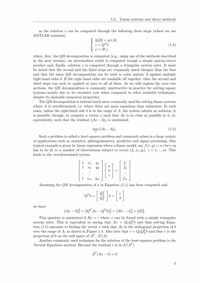
This quantity is minimized if Rx = c where x can be found with a simple triangularsystem solve. This is equivalent to saying that Ax = Q1QT

1 b and thus solving Equa-tion (1.5) amounts to finding the vector x such that Ax is the orthogonal projection of bover the range of A, as shown in Figure 1.4. Also note that r = Q2QT

2 b and thus r is theprojection of b on the null space of AT , N (A).

Another commonly used technique for the solution of the least-squares problem is theNormal Equations method. Because the residual r is in N (AT )

AT (Ax − b) = 0

5

1. Introduction

Figure 1.4: Solution of a least-squares problem.

and, thus, the solution x to Equation (1.5) can be found solving the linear systemAT Ax = AT b. Because AT A is Symmetric Positive Definite (assuming A has full rank),this can be achieved through the Cholesky factorization. Nonetheless, the method basedon the QR factorization is often preferred because the conditioning of AT A is equal to thesquare of the conditioning of A, which may lead to excessive error propagation.

The QR factorization is also commonly used to solve underdetermined systems, i.e.,with more unknowns than equations, which admit infinite solutions. In such cases thedesired solution is the one with minimum 2-norm:

min‖x‖2, Ax = b. (1.6)

The solution of this problem can be achieved computing the QR factorization of AT

[Q1Q2]

[R0

]= AT

where Q1 ∈ Rn × m and Q2 ∈ Rn × (n − m). Then

Ax = RT QT x = [RT 0]

[z1

z2

]= b

and the minimum 2-norm solution follows by setting z2 = 0. Note that Q2 is an orthog-onal basis for N (A) and, thus, the minimum 2-norm solution is computed by removingfor any admissible solution x all of its components in N (A).

For the sake of space and readability, we do not discuss here the use of iterativemethods such as LSQR [91] or Craig [39] for the solution of problems (1.5) and (1.6) butwe refer the reader to the book by Bjorck [23] which contains a thorough description ofthe classical methods used for solving least-squares and minimum 2-norm problems.

1.2.2 QR decomposition

The QR decomposition of a matrix can be computed in different ways; the use of GivensRotations [57], Householder reflections [69] or the Gram-Schmidt orthogonalization [100]are among the most commonly used and best known ones. We will not cover here the use ofGivens Rotations, Gram-Schmidt orthogonalization and their variants and refer, instead,the reader to classic linear algebra textbooks such as Golub et al. [59] or Bjorck [23] for anexhaustive discussion of such methods. We focus, instead, on the QR factorization basedon Householder reflections which has become the most commonly used method especially

6

1.2. Linear systems and direct methods

because of the availability of algorithms capable of achieving very high performance onprocessors equipped with memory hierarchies.

For a given a vector u, a Householder Reflection is defined as

H = I − 2uuT

uT v(1.7)

and u is commonly referred to as Householder vector. It is easy to verify that H issymmetric and orthogonal. Because Pu = uuT

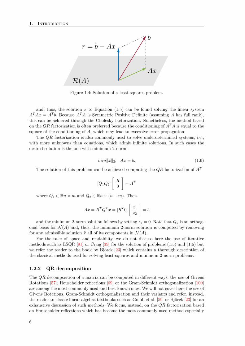
uT uis a projector over the space of u, Hx can

be regarded as the reflection of a vector x on the hyperplane that has normal vector u.This is depicted in Figure 1.5 (left).

Figure 1.5: Householder reflection

The Householder reflection can be defined in such a way that Hx has all zero coefficientsexcept the first, which means to say that Hx = ±‖x‖2e1 where e1 is the first unit vector.This can be achieved if Hx is the reflection of x on the hyperplane that bisects the anglebetween x and ±‖x‖2e1. This hyperplane is orthogonal to the difference of these twovectors x ∓ ‖x‖2e1 which can thus be used to construct the vector

u = x ∓ ‖x‖2e1. (1.8)

Note that, if, for example, x is close to a multiple of e1, then ‖x‖2 ≈ x(1) which maylead to a dangerous cancellation in Equation (1.8); to avoid this problem u is commonlychosen as

u = u + sign(x(1))‖x‖2e1. (1.9)

In practice, it is very convenient to scale u in such a way that its first coefficient isequal to 1 (more on this will be said later). Assuming v = u/u(1), through some simplemanipulations, the Householder transformation H is defined as

H = I − τvvT , where τ =sign(x(1))(x(1) − ‖x‖2)

‖x‖2. (1.10)

Note that the matrix H is never explicitly built neither to store, nor to apply theHouseholder transformation; the storage is done implicitly by means of v and τ and thetransformation can be applied to an entire matrix A ∈ R

m×n in 4mn flops like this

HA = (I − τvvT )A = A − τv(vT A) (1.11)

7

1. Introduction

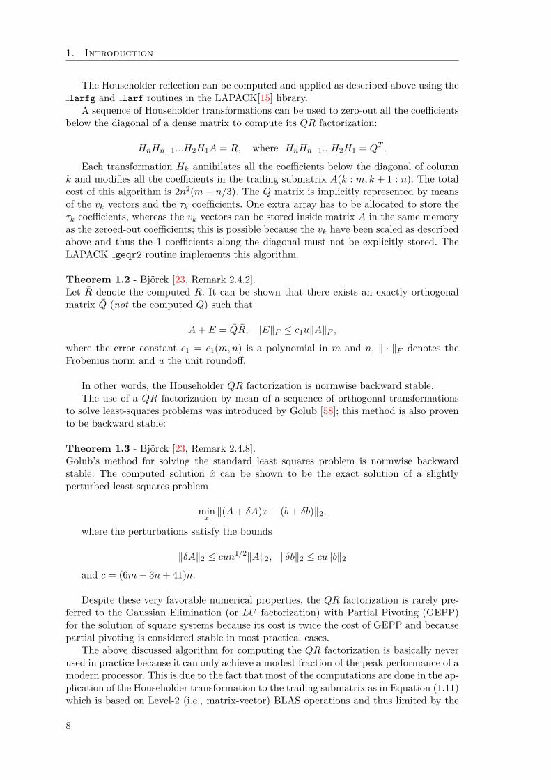
The Householder reflection can be computed and applied as described above using thelarfg and larf routines in the LAPACK[15] library.

A sequence of Householder transformations can be used to zero-out all the coefficientsbelow the diagonal of a dense matrix to compute its QR factorization:

HnHn−1...H2H1A = R, where HnHn−1...H2H1 = QT .

Each transformation Hk annihilates all the coefficients below the diagonal of columnk and modifies all the coefficients in the trailing submatrix A(k : m, k + 1 : n). The totalcost of this algorithm is 2n2(m − n/3). The Q matrix is implicitly represented by meansof the vk vectors and the τk coefficients. One extra array has to be allocated to store theτk coefficients, whereas the vk vectors can be stored inside matrix A in the same memoryas the zeroed-out coefficients; this is possible because the vk have been scaled as describedabove and thus the 1 coefficients along the diagonal must not be explicitly stored. TheLAPACK geqr2 routine implements this algorithm.

Theorem 1.2 - Bjorck [23, Remark 2.4.2].Let R denote the computed R. It can be shown that there exists an exactly orthogonalmatrix Q (not the computed Q) such that

A + E = QR, ‖E‖F ≤ c1u‖A‖F ,

where the error constant c1 = c1(m, n) is a polynomial in m and n, ‖ · ‖F denotes theFrobenius norm and u the unit roundoff.

In other words, the Householder QR factorization is normwise backward stable.The use of a QR factorization by mean of a sequence of orthogonal transformations

to solve least-squares problems was introduced by Golub [58]; this method is also provento be backward stable:

Theorem 1.3 - Bjorck [23, Remark 2.4.8].Golub’s method for solving the standard least squares problem is normwise backwardstable. The computed solution x can be shown to be the exact solution of a slightlyperturbed least squares problem

minx

‖(A + δA)x − (b + δb)‖2,

where the perturbations satisfy the bounds

‖δA‖2 ≤ cun1/2‖A‖2, ‖δb‖2 ≤ cu‖b‖2

and c = (6m − 3n + 41)n.

Despite these very favorable numerical properties, the QR factorization is rarely pre-ferred to the Gaussian Elimination (or LU factorization) with Partial Pivoting (GEPP)for the solution of square systems because its cost is twice the cost of GEPP and becausepartial pivoting is considered stable in most practical cases.

The above discussed algorithm for computing the QR factorization is basically neverused in practice because it can only achieve a modest fraction of the peak performance of amodern processor. This is due to the fact that most of the computations are done in the ap-plication of the Householder transformation to the trailing submatrix as in Equation (1.11)which is based on Level-2 (i.e., matrix-vector) BLAS operations and thus limited by the

8

1.2. Linear systems and direct methods

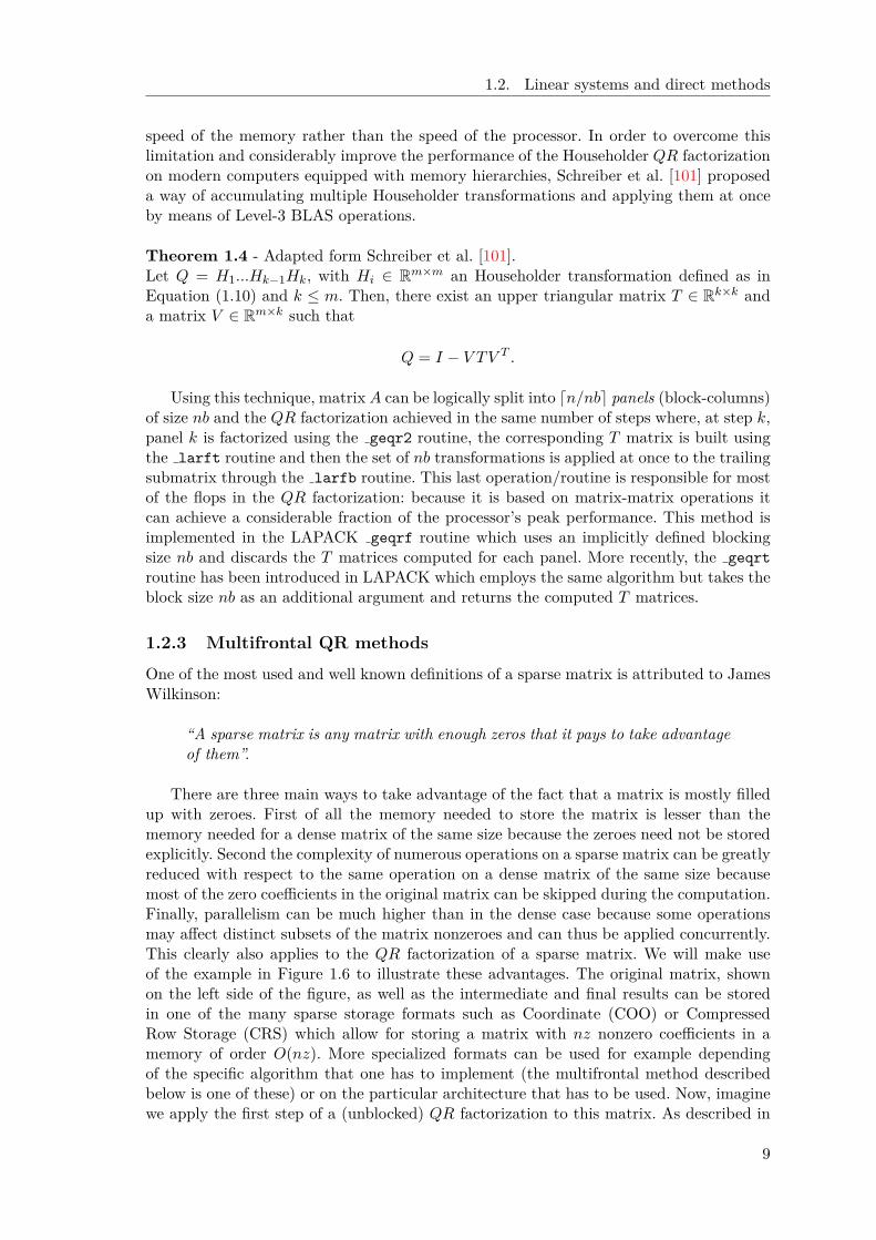
speed of the memory rather than the speed of the processor. In order to overcome thislimitation and considerably improve the performance of the Householder QR factorizationon modern computers equipped with memory hierarchies, Schreiber et al. [101] proposeda way of accumulating multiple Householder transformations and applying them at onceby means of Level-3 BLAS operations.

Theorem 1.4 - Adapted form Schreiber et al. [101].Let Q = H1...Hk−1Hk, with Hi ∈ R

m×m an Householder transformation defined as inEquation (1.10) and k ≤ m. Then, there exist an upper triangular matrix T ∈ R

k×k anda matrix V ∈ R

m×k such that

Q = I − V TV T .

Using this technique, matrix A can be logically split into n/nb panels (block-columns)of size nb and the QR factorization achieved in the same number of steps where, at step k,panel k is factorized using the geqr2 routine, the corresponding T matrix is built usingthe larft routine and then the set of nb transformations is applied at once to the trailingsubmatrix through the larfb routine. This last operation/routine is responsible for mostof the flops in the QR factorization: because it is based on matrix-matrix operations itcan achieve a considerable fraction of the processor’s peak performance. This method isimplemented in the LAPACK geqrf routine which uses an implicitly defined blockingsize nb and discards the T matrices computed for each panel. More recently, the geqrt

routine has been introduced in LAPACK which employs the same algorithm but takes theblock size nb as an additional argument and returns the computed T matrices.

1.2.3 Multifrontal QR methods

One of the most used and well known definitions of a sparse matrix is attributed to JamesWilkinson:

“A sparse matrix is any matrix with enough zeros that it pays to take advantageof them”.

There are three main ways to take advantage of the fact that a matrix is mostly filledup with zeroes. First of all the memory needed to store the matrix is lesser than thememory needed for a dense matrix of the same size because the zeroes need not be storedexplicitly. Second the complexity of numerous operations on a sparse matrix can be greatlyreduced with respect to the same operation on a dense matrix of the same size becausemost of the zero coefficients in the original matrix can be skipped during the computation.Finally, parallelism can be much higher than in the dense case because some operationsmay affect distinct subsets of the matrix nonzeroes and can thus be applied concurrently.This clearly also applies to the QR factorization of a sparse matrix. We will make useof the example in Figure 1.6 to illustrate these advantages. The original matrix, shownon the left side of the figure, as well as the intermediate and final results can be storedin one of the many sparse storage formats such as Coordinate (COO) or CompressedRow Storage (CRS) which allow for storing a matrix with nz nonzero coefficients in amemory of order O(nz). More specialized formats can be used for example dependingof the specific algorithm that one has to implement (the multifrontal method describedbelow is one of these) or on the particular architecture that has to be used. Now, imaginewe apply the first step of a (unblocked) QR factorization to this matrix. As described in

9

1. Introduction

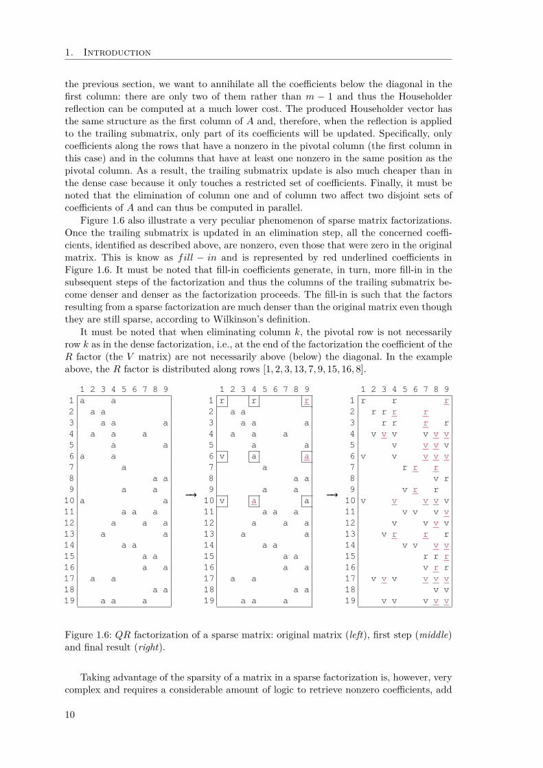
the previous section, we want to annihilate all the coefficients below the diagonal in thefirst column: there are only two of them rather than m − 1 and thus the Householderreflection can be computed at a much lower cost. The produced Householder vector hasthe same structure as the first column of A and, therefore, when the reflection is appliedto the trailing submatrix, only part of its coefficients will be updated. Specifically, onlycoefficients along the rows that have a nonzero in the pivotal column (the first column inthis case) and in the columns that have at least one nonzero in the same position as thepivotal column. As a result, the trailing submatrix update is also much cheaper than inthe dense case because it only touches a restricted set of coefficients. Finally, it must benoted that the elimination of column one and of column two affect two disjoint sets ofcoefficients of A and can thus be computed in parallel.

Figure 1.6 also illustrate a very peculiar phenomenon of sparse matrix factorizations.Once the trailing submatrix is updated in an elimination step, all the concerned coeffi-cients, identified as described above, are nonzero, even those that were zero in the originalmatrix. This is know as fill − in and is represented by red underlined coefficients inFigure 1.6. It must be noted that fill-in coefficients generate, in turn, more fill-in in thesubsequent steps of the factorization and thus the columns of the trailing submatrix be-come denser and denser as the factorization proceeds. The fill-in is such that the factorsresulting from a sparse factorization are much denser than the original matrix even thoughthey are still sparse, according to Wilkinson’s definition.

It must be noted that when eliminating column k, the pivotal row is not necessarilyrow k as in the dense factorization, i.e., at the end of the factorization the coefficient of theR factor (the V matrix) are not necessarily above (below) the diagonal. In the exampleabove, the R factor is distributed along rows [1, 2, 3, 13, 7, 9, 15, 16, 8].

1 2 3 4 5 6 7 8 9

1 a a

2 a a

3 a a a

4 a a a

5 a a

6 a a

7 a

8 a a

9 a a

10 a a

11 a a a

12 a a a

13 a a

14 a a

15 a a

16 a a

17 a a

18 a a

19 a a a

��

1 2 3 4 5 6 7 8 9

1 r r r

2 a a

3 a a a

4 a a a

5 a a

6 v a a

7 a

8 a a

9 a a

10 v a a

11 a a a

12 a a a

13 a a

14 a a

15 a a

16 a a

17 a a

18 a a

19 a a a

��

1 2 3 4 5 6 7 8 9

1 r r r

2 r r r r

3 r r r r

4 v v v v v v

5 v v v v

6 v v v v v

7 r r r

8 v r

9 v r r

10 v v v v v

11 v v v v

12 v v v v

13 v r r r

14 v v v v

15 r r r

16 v r r

17 v v v v v v

18 v v

19 v v v v v

Figure 1.6: QR factorization of a sparse matrix: original matrix (left), first step (middle)and final result (right).

Taking advantage of the sparsity of a matrix in a sparse factorization is, however, verycomplex and requires a considerable amount of logic to retrieve nonzero coefficients, add

10

1.2. Linear systems and direct methods

new ones, identify tasks that can be performed in parallel etc. Graph theory can assistin achieving these tasks as it allows for computing matrix permutations that reduce thefill-in, computing the number and position of fill-in coefficients, defining the dependenciesbetween the elimination steps of the factorization. All this information is commonly com-puted in a preliminary phase, commonly referred to as analysis whose cost is O(|A|+ |R|)where |A| and |R| are, respectively, the number of nonzeroes in A and R. We refer thereader to classic textbooks on direct, sparse methods such as the ones by Duff et al. [48] orDavis [41] for a thorough description of the techniques used in the analysis phase. One thissymbolic, structural information is available upon completion of the analysis, the actualfactorization can take place using different techniques. For the sparse QR factorization,the most commonly employed technique is the multifrontal method which was first intro-duced by Duff and Reid [49] as a method for the factorization of sparse, symmetric linearsystems. At the heart of this method is the concept of an elimination tree, introduced bySchreiber [102] and extensively studied and formalized later by Liu [84]. This tree graph,computed at the analysis phase, describes the dependencies among computational tasksin the multifrontal factorization. The multifrontal method can be adapted to the QR fac-torization of a sparse matrix thanks to the fact that the R factor of a matrix A and theCholesky factor of the normal equation matrix AT A share the same structure under thehypothesis that the matrix A is Strong Hall:

Definition 1.1 - Strong Hall matrix [23, Definition 6.4.1].A matrix A ∈ R

m×n, m ≥ n is said to have the Strong Hall property if every subset ofk columns, 0 < k < n, the corresponding submatrix has nonzeroes in at leas k + 1 rows.

Based on this equivalence, the structure of the R factor of A is the same as that of theCholesky factor of AT A (excluding numerical cancellations) and the elimination tree forthe QR factorization of A is the same as that for the Cholesky factorization of AT A. Inthe case where the Strong Hall property does not hold, the elimination tree related to theCholesky factorization of AT A can still be used although the resulting QR factorizationwill perform more computations and consume more memory than what is really needed;alternatively, the matrix A can be permuted to a Block Triangular Form (BTF) where allthe diagonal blocks are Strong Hall.

In a basic multifrontal method, the elimination tree has n nodes, where n is the numberof columns in the input matrix A, each node representing one pivotal step of the QRfactorization of A. This tree is defined by a parent relation where the parent of node iis equal to the index of the first off-diagonal coefficient in row i of the factor R. Theelimination tree for the matrix in Figure 1.6 is depicted in Figure 1.7. Every node ofthe tree is associated with a dense frontal matrix (or, simply, front) that contains allthe coefficients affected by the elimination of the corresponding pivot. The whole QRfactorization consists in a topological order (i.e., bottom-up) traversal of the tree where,at each node, two operations are performed:

• assembly: a set of rows from the original matrix (all those which have a nonzeroin the pivotal column) is assembled together with data produced by the processingof child nodes to form the frontal matrix. This operation simply consists in stackingthese data one on top of the other: the rows of these data sets can be stacked in anyorder but the order of elements within rows has to be the same. The set of columnindices associated with a node is, in general, a superset of those associated with itschildren;

11

1. Introduction

• factorization: one Householder reflector is computed and applied to the wholefrontal matrix in order to annihilate all the subdiagonal elements in the first column.This step produces one row of the R factor of the original matrix and a complementwhich corresponds to the data that will be later assembled into the parent node(commonly referred to as a contribution block). The Q factor is defined implicitly bymeans of the Householder vectors computed on each front; the matrix that storesthe coefficients of the computed Householder vectors, will be referred to as the Vmatrix from now on.

1 2 3 4 5 6 7 8 9

1 r r r

6 v v v v v

10 v v v v v

2 r r r r

4 v v v v v v

17 v v v v v v

3 r r r r

13 v r r r

19 v v v v v

5 v v v v

12 v v v v

7 r r r

9 v r r

11 v v v v

14 v v v v

15 r r r

16 v r r

8 v r

18 v v

1 2 3 4 5 6 7 8 9

1 r r r

2 r r r r

3 r r r r

13 r r r

7 r r r

9 r r

15 r r r

16 r r

8 r

2

5

4

1 3

9

8

7

6

1

2

43

5

Figure 1.7: Example of multifrontal QR factorization. On the left side the factorized matrix(the same as in Figure 1.6 with a row permutation). On the upper-right part, the structureof the resulting R factor. On the right-bottom part the elimination tree; the dashed boxesshow how the nodes are amalgamated into supernodes.

In practical implementations of the multifrontal QR factorization, nodes of the elimi-nation tree are amalgamated to form supernodes. The amalgamated pivots correspond torows of R that have the same structure and can be eliminated at once within the samefrontal matrix without producing any additional fill-in in the R factor. The elimination ofamalgamated pivots and the consequent update of the trailing frontal submatrix can thusbe performed by means of efficient Level-3 BLAS routines through the WY representa-tion [101]. Moreover, amalgamation reduces the number of assembly operations increasingthe computations-to-communications ratio which results in better performance. The amal-gamated elimination tree is also commonly referred to as assembly tree.

Figure 1.7 shows some details of a sparse QR factorization. The factorized matrix isshown on the left part of the figure. Note that this is the same matrix as in Figure 1.6where the rows of A are sorted in order of increasing index of the leftmost nonzero in orderto show more clearly the computational pattern of the method on the input data. Actually,the sparse QR factorization in insensitive to row permutations which means that any rowpermutation will always yield the same fill-in, as it can be verified comparing Figures 1.6and 1.7. On the top-right part of the figure, the structure of the resulting R factor is shown.

12

1.2. Linear systems and direct methods

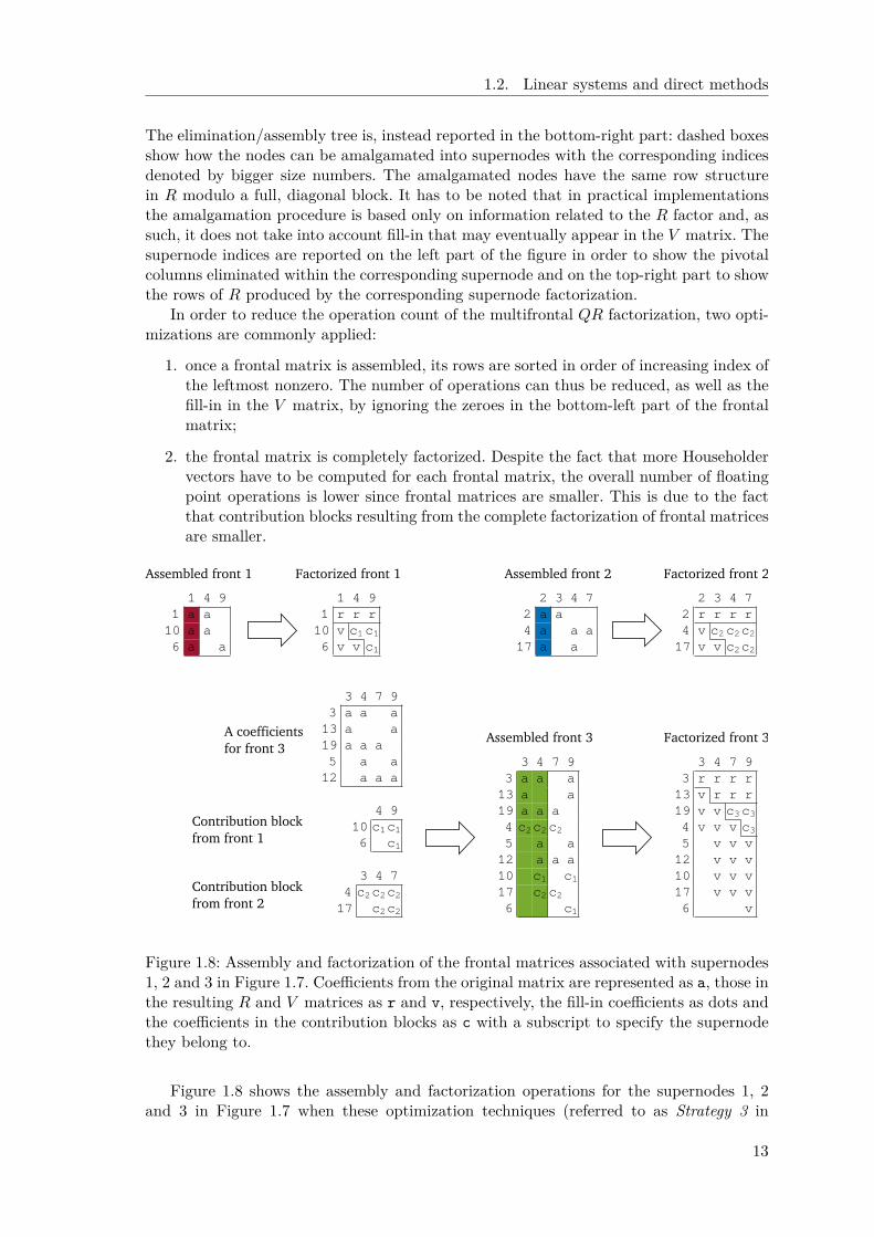
The elimination/assembly tree is, instead reported in the bottom-right part: dashed boxesshow how the nodes can be amalgamated into supernodes with the corresponding indicesdenoted by bigger size numbers. The amalgamated nodes have the same row structurein R modulo a full, diagonal block. It has to be noted that in practical implementationsthe amalgamation procedure is based only on information related to the R factor and, assuch, it does not take into account fill-in that may eventually appear in the V matrix. Thesupernode indices are reported on the left part of the figure in order to show the pivotalcolumns eliminated within the corresponding supernode and on the top-right part to showthe rows of R produced by the corresponding supernode factorization.

In order to reduce the operation count of the multifrontal QR factorization, two opti-mizations are commonly applied:

1. once a frontal matrix is assembled, its rows are sorted in order of increasing index ofthe leftmost nonzero. The number of operations can thus be reduced, as well as thefill-in in the V matrix, by ignoring the zeroes in the bottom-left part of the frontalmatrix;

2. the frontal matrix is completely factorized. Despite the fact that more Householdervectors have to be computed for each frontal matrix, the overall number of floatingpoint operations is lower since frontal matrices are smaller. This is due to the factthat contribution blocks resulting from the complete factorization of frontal matricesare smaller.

1 4 9

1 a a

10 a a

6 a a

1 4 9

1 r r r

10 v c1c1

6 v v c1

2 3 4 7

2 a a

4 a a a

17 a a

2 3 4 7

2 r r r r

4 v c2c2c2

17 v v c2c2

Assembled front 1 Factorized front 1 Assembled front 2 Factorized front 2

3 4 7 9

3 a a a

13 a a

19 a a a

5 a a

12 a a a

3 4 7

4 c2c2c2

17 c2c2

4 9

10 c1c1

6 c1

3 4 7 9

3 a a a

13 a a

19 a a a

4 c2c2c2

5 a a

12 a a a

10 c1 c1

17 c2c2

6 c1

3 4 7 9

3 r r r r

13 v r r r

19 v v c3c3

4 v v v c3

5 v v v

12 v v v

10 v v v

17 v v v

6 v

A coefficients

for front 3

Contribution block

from front 1

Contribution block

from front 2

Assembled front 3 Factorized front 3

Figure 1.8: Assembly and factorization of the frontal matrices associated with supernodes1, 2 and 3 in Figure 1.7. Coefficients from the original matrix are represented as a, those inthe resulting R and V matrices as r and v, respectively, the fill-in coefficients as dots andthe coefficients in the contribution blocks as c with a subscript to specify the supernodethey belong to.

Figure 1.8 shows the assembly and factorization operations for the supernodes 1, 2and 3 in Figure 1.7 when these optimization techniques (referred to as Strategy 3 in

13

1. Introduction

Amestoy et al. [14]) are applied. Note that, because supernodes 1 and 2 are leaves of theassembly tree, the corresponding assembled frontal matrices only include coefficients fromthe matrix A. The contribution blocks resulting from the factorization of supernodes 1and 2 are appended to the rows of the input A matrix associated with supernode 3 insuch a way that the resulting, assembled, frontal matrix has the staircase structure shownin Figure 1.8 (bottom-middle). Once the front is assembled, it is factorized as shown inFigure 1.8 (bottom-right).

A detailed presentation of the multifrontal QR method, including the optimizationtechniques described above, can be found in the work by Amestoy et al. [14] or Davis [41].

The multifrontal method can achieve very high efficiency on modern computing sys-tems because all the computations are arranged as operations on dense matrices; this re-duces the use of indirect addressing and allows the use of efficient Level-3 BLAS routineswhich can achieve a considerable fraction of the peak performance of modern computingsystems.

1.3 Parallelization of the QR factorization

1.3.1 Dense QR factorization

Computing the QR factorization of a dense matrix is a relatively expensive task becauseas explained above, its cost is O(n2m) flops. Therefore, especially when dealing with largesize problems, parallelization is a natural way of reducing the execution time. In addition,due to its high computational intensity (i.e., the number of operations divided by theamount of data manipulated), the QR factorization of a dense matrix can potentiallyachieve a good scaling under favorable circumstances (more on these below).

As explained in Section 1.2.2, the blocked QR factorization is a succession of panelreductions ( geqrt) and update ( gemqrt) operations. The panel reduction is essentiallybased on Level-2 BLAS operations. This means that this operation cannot be efficientlyparallelized because its cost is dominated by data transfers, either from main memory tothe processor, or among processors; moreover, the computation of a Householder reflectorimplies computing the norm of an entire column and therefore, at each internal step of thepanel reduction, if the panel is distributed among multiple processors a heavily penalizingreduction operation has to take place. The trailing submatrix update, instead is very richin Level-3 BLAS operations and is thus an ideal candidate for parallelization because thedata transfers can easily overlapped with computations.

A very classic and straightforward way to parallelize the blocked QR factorizationdescribed in Section 1.2.2 is based on a fork-join model where sequential panel operationsare alternated with parallel updates. This can be easily implemented if the trailing sub-matrix is split into block-columns and each block-column updated by a different processindependently of the others, as in the interior loop of the following pseudocode:

1 do k=1, n/nb

! reduce panel a(k)

3 call _geqrt (a(k))

5 do j=k+1, n/nb

! update block - column a(j) w.r.t. panel a(k)

7 call _gemqrt (a(k), a(j))

end do

9 end do

14

1.3. Parallelization of the QR factorization

The scalability of this approach can be improved noting that it is not necessary towait for the completion of all the updates in step k to compute the reduction of panela(k+1) but this can be started as soon as the update of block-column a(k+1) with respectto panel a(k) is finished. This technique is well known under the name of lookahead andessentially allows for pipelining two consecutive stages of the blocked QR factorization;the same idea can be pushed further in order to pipeline l stages, in which case we talk ofdepth-l lookahead. In the rest of this document we will refer to this approach as the 1Dparallelization. Despite the improvements brought by lookahead, its scalability remainsextremely poor; even if we had enough resources to perform concurrently all the updates ineach stage of the blocked factorization, the execution time will be severely limited by theslow and sequential panel reductions. This is especially true for extremely overdeterminedmatrices where the cost of panel reductions becomes very high relative to the cost ofupdate operations.

For this reason, when multicore architectures started to appear (around the beginningof the 2000s) and the core count of supercomputers started to ramp up, novel algorithmswere introduced to overcome these limitations. These methods, known under the name oftile or communication-avoiding algorithms are based on a 2D decomposition of matricesinto tiles (or blocks) of size nb x nb; this permits to break down the panel factorizationand the related updates into smaller tasks which leads to a three-fold advantage:

1. the panel factorization and the related updates can be parallelized;

2. the updates related to a panel stage can be started before the panel is entirelyreduced;

3. subsequent panel stages can be started before the panel is entirely reduced.

In these 2D (because of the decomposition into square blocks) algorithms, the topmostpanel tile (the one lying on the diagonal) is used to annihilate the others; this can beachieved in different ways. For example, the topmost tile can be first reduced into atriangular tile with a general geqrt LAPACK QR factorization which can then be usedto annihilate the other tiles, one after the other, with tpqrt LAPACK QR factorizations,where t and p stand for triangular and pentagonal, respectively. The panel factorization isthus achieved through a flat reduction tree as shown in Figure 1.10 (left). This approachallows for a better pipelining of the tasks (points 2 and 3 above); in the case of extremelyoverdetermined matrices, however, it provides only a moderate additional concurrencywith respect to the 1D approach because the tasks within a panel stage cannot be executedconcurrently. Another possible approach consists in first reducing all the tiles in the panelinto triangular tiles using geqrt operations; this first stage is embarrassingly parallel.Then, through a binary reduction tree, all the triangular tiles except the topmost oneare annihilated using tpqrt operations, as shown in Figure 1.10 (middle). This secondmethod provides better concurrency but results in a higher number of tasks, some of whichare of very small granularity. Also, in this case a worse pipelining of successive panel stagesis obtained [47]. In practice a hybrid approach can be used where the panel is split intosubsets of size bh: each subset is reduced into a triangular tile using a flat reduction treeand then, the remaining tiles are reduced using a binary tree. This is the technique usedin the PLASMA library [9] and illustrated in Figure 1.10 (right) for the case of bh= 2.Other reduction trees can also be employed; we refer the reader to the work by Dongarraet al. [47] for an excellent survey of such techniques.

It must be noted that these algorithms require some extra flops with respect to thestandard blocked QR factorization [34]; this overhead can be reduced to a negligible levelby choosing and appropriate internal block size of the elementary kernels described above.

15

1. Introduction

1 do k=1, n/nb

! for all the block - columns in the front

3 do i = k, m/nb , bh

call _geqrt (f(k,i))

5 do j=k+1, n/nb

call _gemqrt (f(k,i), f(i,j))

7 end do

! intra - subdomain flat -tree reduction

9 do l=i+1, min(i+bh -1,m/nb)

call _tpqrt (f(i,k), f(l,k))

11 do j=k+1, n/nb

call _tpmqrt (f(l,k), f(i,j), f(l,j))

13 end do

end do

15 end do

do while (bh.le.m/nb -k+1)

17 ! inter - subdomains binary -tree reduction

do i = k, m/nb -bh , 2*bh

19 l = i+bh

if(l.le.m/nb) then

21 call _tpqrt (f(i,k), f(l,k))

do j=k+1, n

23 call _tpmqrt (f(l,k), f(i,j), f(l,j))

end do

25 end if

end do

27 bh = bh*2

end do

29 end do

Figure 1.9: Pseudo-code showing the implementation of the tiled QR.

Figure 1.10: Possible panel reduction trees for the 2D front factorization. On the (left),the case of a flat tree, i.e., with bh= ∞. In the (middle), the case of a binary tree, i.e.,with (bh= 1). On the (right) the case of an hybrid tree with bh= 2.

These communication avoiding algorithms have been the object of numerous theoret-ical studies [21, 22, 29] and have been used to accelerate the dense QR factorization onmulticore systems either in single-node, shared memory settings [10, 61, 31, 34, 35], on dis-tributed memory, multicore parallel machines [47, 44, 105, 116], GPU equipped systems [4,16, 116] and even on Grid environments [8].

16

1.4. Programming models and runtime systems

1.3.2 Sparse QR factorization

As explained in Section 1.2.3, sparsity implies that, when performing an operation on amatrix, it is often possible to identify independent tasks that can be executed concurrently,i.e., sparsity implies parallelism. In sparse, direct solvers and thus, being one of them, inthe multifrontal QR method, this concurrency is expressed by the elimination tree: frontsthat belong to different branches are independent and can thus be treated in any orderand, possibly, in parallel. We refer to this type of parallelism as tree parallelism. Theamount of concurrency available in the tree parallelism clearly depends on the shapeof the tree and on the distribution of the computational load along its branches and,as a consequence, on the sparsity structure of the input matrix. As explained above,prior to its factorization a sparse matrix is permuted in order to reduce the fill-in; theshape of the elimination tree clearly depends on this permutation and, consequently, theamount of tree parallelism does too. Local methods such as Average Minimum Degree [12](AMD) or its column variant COLAMD [40], although capable of reducing the fill-in,commonly lead to deep and rather unbalanced elimination trees where tree parallelismis difficult to exploit, especially in distributed memory systems where load balancing isharder to achieve. Nested-dissection [55] based methods instead, not only are very effectivein reducing fill-in (much better than local methods especially for large scale problems),but also lead to wider (binary) and better balanced elimination trees because the loadbalancing can be taken into account by the dissector selection criterion.

Fronts, although much smaller in size than the input sparse matrix, are not small ingeneral. Some of them may have hundred thousands rows or column and, consequently,their factorization may require a considerable amount of work. This provides a secondsource of concurrency which is commonly referred to as front or node parallelism. Any ofthe algorithms presented in the previous section can be used to factorize a frontal matrixusing multiple processes.

The degree of concurrency in tree and node parallelism changes during the bottom-uptraversal of the tree. Fronts are relatively small at the leaf nodes of the tree and growbigger towards the root node; as a result, front parallelism is scarce at the bottom ofthe tree and abundant at the top. On the other hand, tree parallelism provides a highamount of concurrency at the bottom of the tree and only a little at the top part where thetree shrinks towards the root node. Because of this complementarity, using both types ofparallelism is essential for achieving a good scalability. This is clearly much more difficultin the distributed memory parallel case where a careful mapping of processes to tree andnode parallelism has to be done.

1.4 Programming models and runtime systems

Computing platform hardware has dramatically evolved ever since the computer sciencebegan, always striving to provide new convenient accelerating features. Each new accel-erating hardware feature inevitably leaves programmers to decide whether to make theirapplication dependent on that feature (and break compatibility) or not (and miss thepotential benefit), or even to handle both cases (at the cost of extra management code inthe application). This common problem is known as the performance portability issue.

The first purpose of runtime systems is thus to provide abstraction. Runtime systems of-fer a uniform programming interface for a specific subset of hardware (e.g., OpenGL or Di-rectX are well-established examples of runtime systems dedicated to hardware-acceleratedgraphics) or low-level software entities (e.g., POSIX-thread implementations). They aredesigned as thin user-level software layers that complement the basic, general purpose

17

1. Introduction

functions provided by the operating system calls. Applications then target these uniformprogramming interfaces in a portable manner. Low-level, hardware dependent details arehidden inside runtime systems. The adaptation of runtime systems is commonly handledthrough drivers. The abstraction provided by runtime systems thus enables portability.Abstraction alone is however not enough to provide portability of performance, as it doesnothing to leverage low-level-specific features to get increased performance.

Consequently, the second role of runtime systems is to optimize abstract applicationrequests by dynamically mapping them onto low-level requests and resources as efficientlyas possible. This mapping process makes use of scheduling algorithms and heuristics todecide the best actions to take for a given metric and the application state at a givenpoint in its execution time. This allows applications to readily benefit from availableunderlying low-level capabilities to their full extent without breaking their portability.Thus, optimization together with abstraction allows runtime systems to offer portabilityof performance.

In the specific case of parallel work mapping, other approaches have occasionally beenadopted instead of using runtimes. Many scientific applications and libraries, includinglinear system solvers, integrate their own, customized dynamic scheduling algorithms oreven resort to static scheduling techniques, either for historical reasons, or to avoid thepotential overhead of an extra runtime layer.

However, as multicore processors densify, as cache and memory hierarchies deepen,the resulting increase in complexity now makes the use of work-mapping runtime systemsvirtually unavoidable. Such work-mapping runtime systems take elementary task descrip-tions and dependencies as input and are responsible for dynamically scheduling the taskson available computing units so as to minimize a given cost function (usually the executiontime) under some pre-defined set of constraints.

Work-mapping runtime systems themselves are now facing new challenges with therecent move of the high performance community towards the use of specialized acceleratingcores together with traditional general-purpose cores. They not only have to decide aboutthe interest (or not) to use some specific hardware features, but also have to decide whethersome entire application tasks should rather be performed on an accelerated core or is betterleft on a standard core.

In the case where specialized cores are located on an expansion card having its ownmemory (e.g., most existing GPUs), the input data of a task have to be copied from centralmemory to the card memory before the task can be run. The output results must also becopied back to the central memory once the task computation is complete. The cost ofcopying data between central memory and accelerator memory is not negligible. This cost,as well as data dependencies between tasks, must therefore also be taken into accountby the scheduling algorithms when deciding whether to offload a given task, to avoidunnecessary data transfers. Transfers should also be done in advance and asynchronouslyso as to overlap communication with computation.

1.4.1 Programming models for task-based applications

Modern task-based runtime systems aim at abstracting the low-level details of the hard-ware achitechture and enhance the portability of the performance of the code designed ontop of them. As it is the case in this thesis, in most cases, this abstraction relies on a DAGof tasks. In this DAG, vertices represent the tasks to be executed while edges representthe dependences between them.

While tasks are almost systematically explicitly encoded, runtime systems offer mul-tiple ways to encode the dependencies of the DAG. Each runtime system usually comes

18

1.4. Programming models and runtime systems

Figure 1.11: Pseudo-code (left) and associated DAG (right). Arguments correspondingto data that are modified by the function are underlined. The id1 → id3 dependency isdeclared explicitly while the id1 → id2 dependency is implicitly inferred with respect tothe data hazard on x.

with its own API which includes one or multiple ways to encode the dependencies andtheir exhaustive listing would be out of the scope of this thesis. However, we may con-sider that there are two main modes for encoding dependencies. The most natural methodconsists in declaring explicit dependencies between tasks. In spite of the simplicity of theconcept, this approach may have a limited productivity in practice as some algorithmsmay have dependencies that are difficult to express. Alternatively, dependencies may beimplitcly computed by the runtime system thanks to the sequential consistency. In thislatter approach, tasks are provided in sequence and the data they operate on are alsodeclared.

We illustrate these two dominant modes of expression of dependencies with a simpleexample relying on a minimum number of pseudo-instructions. Assume we want to en-code the DAG shown in Figure 1.4.1 (right) relying on an explicit dependency betweentasks id1 and id3 and an implicit dependency between tasks id1 and id2. A task can bedefined as an instance of a function working on a specific set of data, different taskspossibly being different instances of a same function. For instance, in our example weassume that tasks id1 and id3 are instances of function fun1 while task id2 is an instanceof function fun2. While tasks are instanciated with the submit task pseudo-instruction(see Figure 1.4.1, left), the explicit dependency between tasks id1 and id3 can simply beencoded with a declare dependency pseudo-instruction (see Figure 1.4.1, left). On theother hand, implicit dependencies aim letting the runtime system automatically infer de-pendencies thanks to so-called superscalar analysis [11] which aims at ensuring that theparallelization does not violate dependencies, following the sequential consistency. WhileCPUs implement such a superscalar analysis on chip at the instruction level [11], run-time systems implement it in a software layer on tasks. Superscalar analysis is performedon tasks and the associated input/output data they operate on. Assume that task id1

operates on data x and y in read/write mode and read mode (calling fun1(x, y) if thearguments corresponding to data which are modified by a function are underlined), re-spectively, while task id2 operates on data x in read mode (fun2(x)). Because of possibledata hazards occurring on x between tasks id1 and id2, the superscalar analysis detectsthat a dependency is required to respect the sequential consistency.

Another important paradigm for handling dependencies consists of recursive submis-sion. Indeed, it may be convenient for the programmer to let tasks trigger other tasks.Sometimes, one may furthermore need the task to be fully completed and cleaned up be-fore triggering other tasks. Runtime systems often support this option through a so-calledcall-back mechanism consisting of a post-processing portion of code executed once the taskis completed and cleaned up.

Depending on the context, the programmer affinity and portion of the algorithm toencode, different paradigms may be considered as natural and appropriate. For instance,

19

1. Introduction

we propose and study a task-based multifrontal method relying a combination of thesefour types of dependencies (explicit, implicit, recursive, call-back) in Section 3.2.1 in or-der to reproduce as accurately as possible the behavior of the original qr mumps codewith a general purpose runtime system. Although relatively natural to write as it followsthe trends of the original code, the resulting task-based code is complex and difficult tomaintain because it relies on multiple paradigms for handling dependencies. Alternatively,one may rely on a well-defined and more simple programming model in order to design arelatively more simple code, easier to maintain and benefit from properties provided bythe model. The Sequential Task Flow (STF) programming model consists on fully relyingon sequential consistency using only implicit dependencies. The STF model, there-fore, consists of submitting a sequence of tasks through a non blocking function call thatdelegates the execution of the task to the runtime system. Upon submission, the runtimesystem adds the task to the current DAG along with its dependencies which are automati-cally computed through data dependency analysis [11]. The actual execution of the task isthen postponed to the moment when its dependencies are satisfied. As mentioned above,this paradigm is also sometimes referred to as superscalar since it mimics the functioningof superscalar processors where instructions are issued sequentially from a single streambut can actually be executed in a different order and, possibly, in parallel depending ontheir mutual dependencies. We propose and study the design of a multifrontal methodbased on this model in Chapter 4. We show that the simplicity of the model allows for de-signing more advanced numerical algorithms with an concise yet effective expression. Wealso rely on properties we can derive from the model in order to design a memory-awaremechanism in Chapter 5 and extend the scope of the method to heterogeneous platformsin Chapter 6.

One challenge in scaling to large scale many-core systems is how to represent extremelylarge DAGs of tasks in a compact fashion. Cosnard et al. [38] presented a model, namely theParameterized Task Graph (PTG), which addresses this issue. In this model, tasks are notenumerated but parametrized and dependencies between tasks are explicit. For instance,in the DAG represented in Figure 1.4.1 (right), tasks id1 and id3 are two instances of thesame type of task implementing fun1. This property can be used to encode the DAG in acompact way inducing a lower memory footprint for its representation as well as ensuringlimited complexity for parsing it while the problem size grows. For this reason the memoryconsumption overhead in the runtime system for representing the DAG can much lowerfor the PTG model than for the STF model. In addition with a STF model the DAG hasto be completely unrolled whereas with a PTG the DAG is only partially unfolded duringthe execution following the task progression. From this point of view, the advantage of thePTG approach over the STF one can be crucial in a distributed memory context becausethe DAG is pruned on every nodes and only a portion of the DAG is represented on eachnodes. This could considerably reduce the runtime overhead for the management of theDAG. On the other hand, knowing the entire DAG can be useful to compute the scheduleof the DAG or give information to the dynamic scheduler by prepossessing the DAG. Forthese reasons we discuss the potential advantages of relying on such a model for designinga multifrontal method in Section 7.1.

1.4.2 Task-based runtime systems for modern architectures

Many initiatives have emerged in the past years to develop efficient runtime systemsfor modern heterogeneous platforms. Most of these runtime systems use a task-basedparadigm to express concurrency and dependencies by employing a task dependency graphto represent the application to be executed. The main differences between all the ap-

20

1.4. Programming models and runtime systems

proaches are related, to the programming model, to whether or not they manage datamovements between computational resources and to which extent they focus on taskscheduling.

Some runtime systems have been specifically designed for the development of parallellinear algebra applications. One of these if the TBLAS runtime system [106], which pro-vides a simple interface to create dense linear algebra applications and automates datatransfers. TBLAS assumes that programmers should statically map data on the differentprocessing units but it supports heterogeneous data block sizes (i.e., different granularityof computations). The QUARK runtime system [79] was specifically designed for schedul-ing linear algebra kernels on multi-core architectures. It is characterized by a schedulingalgorithm based on work-stealing and by its higher scalability in comparison with otherdedicated runtime systems. Finally, the SuperMatrix runtime system [37], follows nearlythe same idea as it represents the matrix hierarchically: the matrix is viewed as blocksthat serve as units of data where operations over those blocks are treated as units of com-putation. The implementation transparently enqueues the required operations, internallytracking dependencies, and then executes the operations utilizing out-of-order executiontechniques.

Most of the available runtime systems, however, do not target any specific type ofapplications and provide a general API. Qilin [87], for example, provides an interface tosubmit kernels that operate on arrays which are automatically dispatched between the dif-ferent processing units of an heterogeneous machine. Moreover, Qilin dynamically compilesparallel code for both CPUs (by relying on the Intel TBB [95] technology) and for GPUs,using CUDA. Another relevant framework is Charm++ [75] which is a parallel variant ofthe C++ language that provides sophisticated load balancing and a large number of com-munication optimization mechanisms. Charm++ has been extended to provide supportfor accelerators such as the Cell processors as well as GPUs [78]. Many runtime systemspropose a task-based programming paradigm. Runtime systems like KAAPI/XKAAPI [53]or APC+ [62], Legion [31], Realm [112] offer support for hybrid platforms mixing CPUsand GPUs. Their data management is based on a DSM-like mechanism: each data block isassociated with a bitmap that permits to determine whether there is already a copy locallyavailable to a specific processing unit or not. Moreover, task scheduling within KAAPIis based on work-stealing mechanisms or on graph partitioning. The StarSs project isactually an umbrella term that describes both the StarSs language extensions and a col-lection of runtime systems targeting different types of platforms [20, 19]. StarSs providesan annotation-based language which extends C or Fortran applications to offload piecesof computation on the architecture targeted by the underlying runtime system. The PaR-SEC [26, 25] (formerly DAGuE) runtime system dynamically schedules tasks within a nodeusing a rather simple strategy based on a locality-aware work-stealing strategy. It was firstintroduced for linear algebra but was later extended to more generic applications. It takesadvantage of the specific shape of the task graphs (in the sense that there are few typesof tasks) to represent the task dependency graph in an algebraic fashion. More detailson this tool are given in Section 1.4.2.2 The StarPU runtime system provides a genericinterface for developing parallel, task-based applications. It supports multicore architec-tures equipped with accelerator as well as distributed memory systems. This runtime iscapable of transparently handling data and provides a rich panel of features. The detailsof this runtime systems are given in Section 1.4.2.1. All the above mentioned efforts havecontributed to proving the ease of use, the effectiveness and portability of general purposeruntime systems to the point where the OpenMP board has decided to include similarfeatures in the latest OpenMP standard 4.0: the task construct was extended with thedepend clause which enables the OpenMP runtime to automatically detect dependencies

21

1. Introduction

among tasks and consequently schedule them. The same OpenMP standard also providesconstructs for using accelerator devices.

Whereas task-based runtime systems were mainly research tools in the past years,their recent progress makes them now solid candidates for designing advanced scientificsoftware as they provide programming paradigms that allow the programmer to expressconcurrency in a simple yet effective way and relieve him from the burden of dealing withlow-level architectural details.

The work presented in this thesis relies on the StarPU runtime system. This is mostlydue to its large set of features which include full control over the scheduling policy, supportfor accelerators and distributed memory parallelism and transparent handling of data. Forthis reason, this runtime is described in more details in Section 1.4.2.1. Part of our workis also focused on evaluating the use of the PaRSEC runtime system for the implemen-tation of the multifrontal QR factorization. This runtime supports a radically differentprogramming model with respect to StarPU; more details can be found in Section 1.4.2.2.

1.4.2.1 The StarPU runtime system

StarPU is a runtime system developed by the STORM (formerly RUNTIME) team atInria Bordeaux specifically designed for the parallelization of algorithms on heterogeneousarchitectures. A complete description of StarPU can be found in the work by Augonnetet al. [18].

StarPU provides an interface which is extremely convenient for implementing andparallelizing applications or algorithms that can be described as a graph of tasks. Taskshave to be explicitly submitted to the runtime system along with the data they work on andthe corresponding data access mode. Through data analysis, StarPU can automaticallydetect the dependencies among tasks and build the corresponding DAG. Once a task issubmitted, the runtime tracks its dependencies and schedules its execution as soon asthese are satisfied, taking care of gathering the data on the unit where the task is actuallyexecuted. In StarPU the execution is initiated by a master thread, running on a CPU,which is commonly in charge of submitting the tasks; the execution of the tasks, instead,is performed by worker threads (or, simply, workers) whose number and type (e.g., CPUor GPU) can be chosen by the programmer or by the user at run time. A CPU worker isbound to a CPU core whereas a GPU worker is bound to a GPU and a CPU core whichis used to drive the work of the GPU. Note that nothing prevents worker threads fromsubmitting tasks although this does not comply with the Sequential Task Flow model.Because StarPU has full control over a task and the associated data, these have to bedeclared to the runtime prior to the task submission. A task type can be declared througha codelet which specifies, among other things, the name of the task type, the units whereit can be executed (e.g., CPU and/or GPU), the corresponding implementations (onefor each type of unit) and the number of input data. Data, instead, is declared througha specific function call where the programmer informs StarPU about the location of thedata (i.e., the data pointer) and about its properties such as the size, the rank, the leadingdimension. Upon execution of this function call, StarPU returns a handle; once declaredthe data is not meant to be directly accessed by the programmer anymore but only throughthe handle and the associated methods. A task can roughly be defined as an instance of atask type coupled with a set of handles which represent the data used by the task itself.

We can more conveniently illustrate the functioning of StarPU using the simple se-quential code in Figure 1.12 as an example. The purpose of the sequential example is tocompute every elements of the array denoted y, using the input array x. The computationis done by applying the functions f, g as shown in the example. The right side of the figure

22

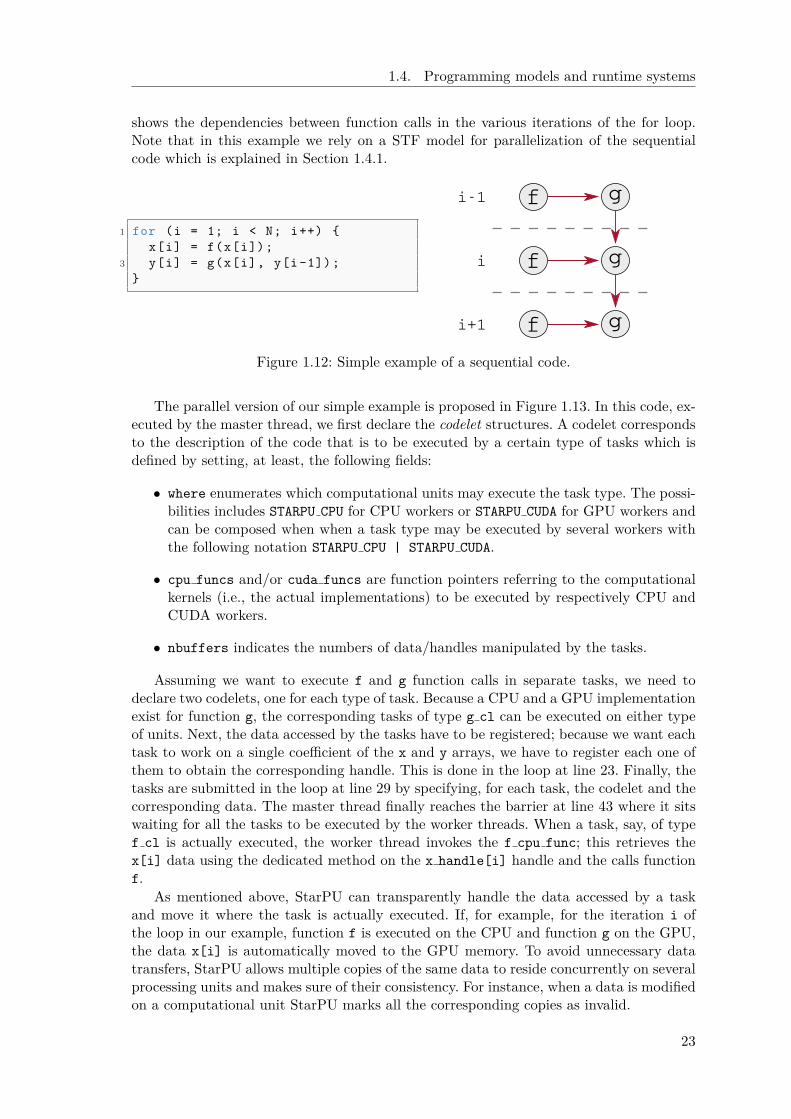
1.4. Programming models and runtime systems

shows the dependencies between function calls in the various iterations of the for loop.Note that in this example we rely on a STF model for parallelization of the sequentialcode which is explained in Section 1.4.1.

1 for (i = 1; i < N; i++) {

x[i] = f(x[i]);

3 y[i] = g(x[i], y[i -1]);

}f g

f g

f g

i-1

i

i+1

Figure 1.12: Simple example of a sequential code.

The parallel version of our simple example is proposed in Figure 1.13. In this code, ex-ecuted by the master thread, we first declare the codelet structures. A codelet correspondsto the description of the code that is to be executed by a certain type of tasks which isdefined by setting, at least, the following fields:

• where enumerates which computational units may execute the task type. The possi-bilities includes STARPU CPU for CPU workers or STARPU CUDA for GPU workers andcan be composed when when a task type may be executed by several workers withthe following notation STARPU CPU | STARPU CUDA.

• cpu funcs and/or cuda funcs are function pointers referring to the computationalkernels (i.e., the actual implementations) to be executed by respectively CPU andCUDA workers.

• nbuffers indicates the numbers of data/handles manipulated by the tasks.

Assuming we want to execute f and g function calls in separate tasks, we need todeclare two codelets, one for each type of task. Because a CPU and a GPU implementationexist for function g, the corresponding tasks of type g cl can be executed on either typeof units. Next, the data accessed by the tasks have to be registered; because we want eachtask to work on a single coefficient of the x and y arrays, we have to register each one ofthem to obtain the corresponding handle. This is done in the loop at line 23. Finally, thetasks are submitted in the loop at line 29 by specifying, for each task, the codelet and thecorresponding data. The master thread finally reaches the barrier at line 43 where it sitswaiting for all the tasks to be executed by the worker threads. When a task, say, of typef cl is actually executed, the worker thread invokes the f cpu func; this retrieves thex[i] data using the dedicated method on the x handle[i] handle and the calls functionf.

As mentioned above, StarPU can transparently handle the data accessed by a taskand move it where the task is actually executed. If, for example, for the iteration i ofthe loop in our example, function f is executed on the CPU and function g on the GPU,the data x[i] is automatically moved to the GPU memory. To avoid unnecessary datatransfers, StarPU allows multiple copies of the same data to reside concurrently on severalprocessing units and makes sure of their consistency. For instance, when a data is modifiedon a computational unit StarPU marks all the corresponding copies as invalid.

23

1. Introduction

/* Codelet definition for kernel f */

2 struct starpu_codelet f_cl =

{

4 .where = STARPU_CPU ,

. cpu_funcs = { f_cpu_func },

6 . nbuffers = 1

};

8

/* Codelet definition for kernel g */

10 struct starpu_codelet g_cl =

{

12 .where = STARPU_CPU | STARPU_CUDA ,

. cpu_funcs = { g_cpu_func },

14 . cuda_funcs = { g_cuda_func },

. nbuffers = 3

16 };

18 starpu_data_handle_t x_handle [N], y_handle [N];

20 starpu_init ();

22 /* declaration of data handles */

for (i = 0; i < N; i++) {

24 starpu_variable_data_register (& x_handle [i], STARPU_MAIN_RAM , (

uintptr_t ) &x[i], sizeof ( double ));

starpu_variable_data_register (& y_handle [i], STARPU_MAIN_RAM , (

uintptr_t ) &y[i], sizeof ( double ));

26 }

28 /* tasks submission */

for (i = 1; i < N; i++) {

30

starpu_insert_task (&f_cl ,

32 STARPU_RW , x_handle [i],

0);

34

starpu_insert_task (&g_cl ,

36 STARPU_R , x_handle [i],

STARPU_R , y_handle [i-1],

38 STARPU_W , y_handle [i],

0);

40

}

42

starpu_task_wait_for_all ();

44

starpu_shutdown ();

Figure 1.13: Simple example of a parallel version of the sequential code in Figure 1.12using a STF model with StarPU.

Among the other features of the StarPU runtime system, in the work described in thefollowing chapters, we will use the following:

24

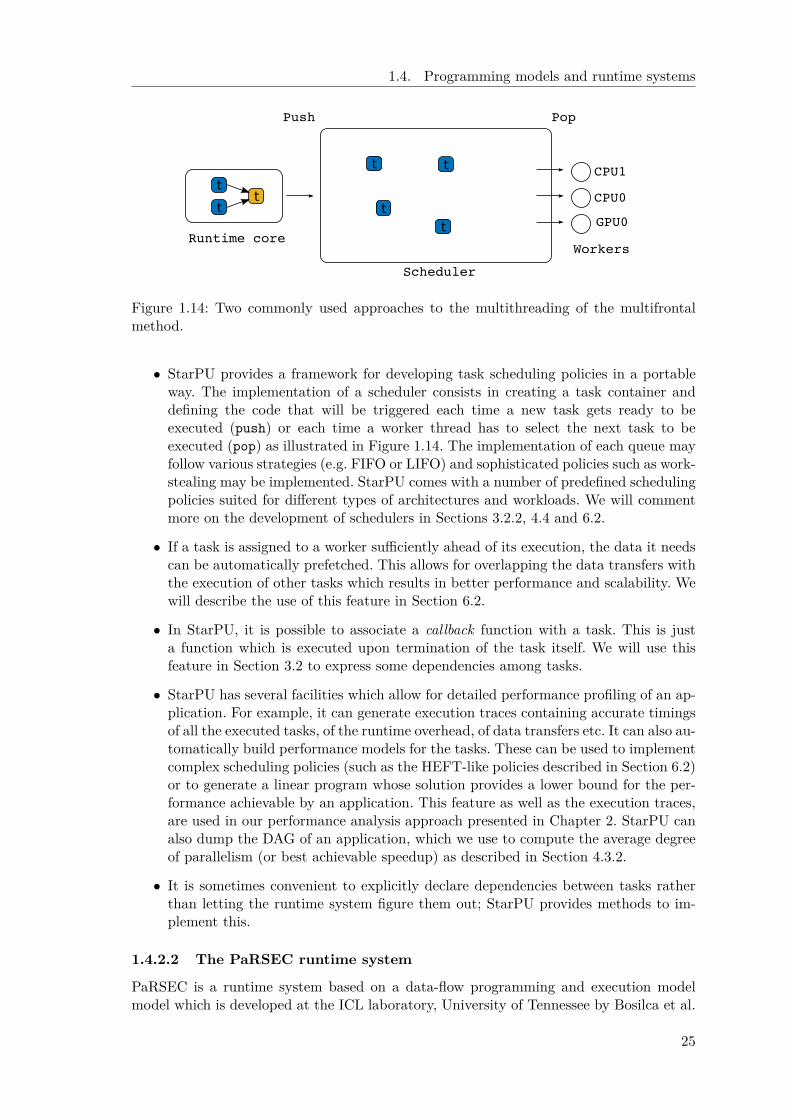
1.4. Programming models and runtime systems

Figure 1.14: Two commonly used approaches to the multithreading of the multifrontalmethod.

• StarPU provides a framework for developing task scheduling policies in a portableway. The implementation of a scheduler consists in creating a task container anddefining the code that will be triggered each time a new task gets ready to beexecuted (push) or each time a worker thread has to select the next task to beexecuted (pop) as illustrated in Figure 1.14. The implementation of each queue mayfollow various strategies (e.g. FIFO or LIFO) and sophisticated policies such as work-stealing may be implemented. StarPU comes with a number of predefined schedulingpolicies suited for different types of architectures and workloads. We will commentmore on the development of schedulers in Sections 3.2.2, 4.4 and 6.2.

• If a task is assigned to a worker sufficiently ahead of its execution, the data it needscan be automatically prefetched. This allows for overlapping the data transfers withthe execution of other tasks which results in better performance and scalability. Wewill describe the use of this feature in Section 6.2.

• In StarPU, it is possible to associate a callback function with a task. This is justa function which is executed upon termination of the task itself. We will use thisfeature in Section 3.2 to express some dependencies among tasks.

• StarPU has several facilities which allow for detailed performance profiling of an ap-plication. For example, it can generate execution traces containing accurate timingsof all the executed tasks, of the runtime overhead, of data transfers etc. It can also au-tomatically build performance models for the tasks. These can be used to implementcomplex scheduling policies (such as the HEFT-like policies described in Section 6.2)or to generate a linear program whose solution provides a lower bound for the per-formance achievable by an application. This feature as well as the execution traces,are used in our performance analysis approach presented in Chapter 2. StarPU canalso dump the DAG of an application, which we use to compute the average degreeof parallelism (or best achievable speedup) as described in Section 4.3.2.

• It is sometimes convenient to explicitly declare dependencies between tasks ratherthan letting the runtime system figure them out; StarPU provides methods to im-plement this.

1.4.2.2 The PaRSEC runtime system

PaRSEC is a runtime system based on a data-flow programming and execution modelmodel which is developed at the ICL laboratory, University of Tennessee by Bosilca et al.

25

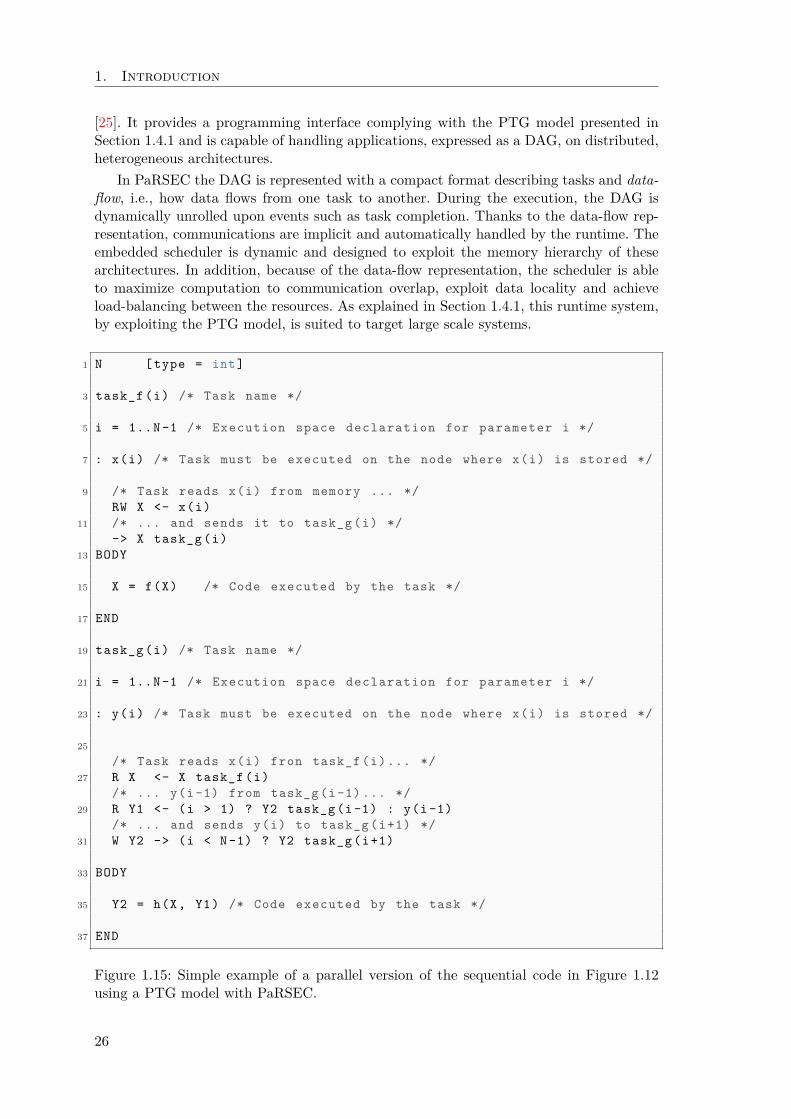
1. Introduction

[25]. It provides a programming interface complying with the PTG model presented inSection 1.4.1 and is capable of handling applications, expressed as a DAG, on distributed,heterogeneous architectures.

In PaRSEC the DAG is represented with a compact format describing tasks and data-flow, i.e., how data flows from one task to another. During the execution, the DAG isdynamically unrolled upon events such as task completion. Thanks to the data-flow rep-resentation, communications are implicit and automatically handled by the runtime. Theembedded scheduler is dynamic and designed to exploit the memory hierarchy of thesearchitectures. In addition, because of the data-flow representation, the scheduler is ableto maximize computation to communication overlap, exploit data locality and achieveload-balancing between the resources. As explained in Section 1.4.1, this runtime system,by exploiting the PTG model, is suited to target large scale systems.

1 N [type = int]

3 task_f (i) /* Task name */

5 i = 1..N-1 /* Execution space declaration for parameter i */

7 : x(i) /* Task must be executed on the node where x(i) is stored */

9 /* Task reads x(i) from memory ... */

RW X <- x(i)

11 /* ... and sends it to task_g (i) */

-> X task_g (i)

13 BODY

15 X = f(X) /* Code executed by the task */

17 END

19 task_g (i) /* Task name */

21 i = 1..N-1 /* Execution space declaration for parameter i */

23 : y(i) /* Task must be executed on the node where x(i) is stored */

25

/* Task reads x(i) fron task_f (i)... */

27 R X <- X task_f (i)

/* ... y(i -1) from task_g (i -1) ... */

29 R Y1 <- (i > 1) ? Y2 task_g (i -1) : y(i -1)

/* ... and sends y(i) to task_g (i+1) */

31 W Y2 -> (i < N -1) ? Y2 task_g (i+1)

33 BODY

35 Y2 = h(X, Y1) /* Code executed by the task */

37 END

Figure 1.15: Simple example of a parallel version of the sequential code in Figure 1.12using a PTG model with PaRSEC.

26

1.5. Related work on dense linear algebra

PaRSEC provides a language called Job Data Flow (JDF) to express PTG parallelcodes. During the compilation process, the files containing the JDF code are translatedinto C-code files by a specific compiler distributed with PaRSEC called daguepp. The DAGis defined by a set of task types that can be associated with several parameters defined ona given range of values. The tasks are associated with a list of predecessors and successorsthat define the dependencies in the DAG. These dependencies are generally based on databut may also represent precedence constraints. Tasks are associated with a code that willbe executed for each task instances. A code specific to different types of resources, suchas CPU or GPU, may be given.

We illustrate the features provided by PaRSEC using the same sequential example usedin the previous section to introduce StarPU. A PTG parallel version of the sequential codein Figure 1.12 is shown in Figure 1.15, using the JDF language. For the sake of brevity weonly show the PTG representation of our example and we do not present the declarationof data types or the instantiation of the DAG from the JDF.

In our JDF we define two different type of tasks, namely task f and task g, thatare associated with the parameter i. This parameter is defined on the ranges 0..N-1 fortask f and 1..N-1 for task g. The parameter N defined at the beginning of the JDFcode, associated with a type, int in our example, and set when the DAG is instantiated.The data-flow associated with task task f contains two edges. The first one reads datax(i) from memory in a variable referred to as X. The second edge send the modified dataX to task task g(i). The data-flow associated with task task g has three edges. Thefirst incoming edge consists in retrieving the data X modified by task task f(i). Thesecond incoming edges retrieved the data called Y1 necessary to compute Y2. For this datawe consider two cases. If i > 1 then Y1 is retrieved from the computed data Y2 in tasktask g(i-1) and otherwise it is read in memory. Finally Y2 is send to tasks task g(i+1)

in the case where such task exists.

Note that the expression of the DAG presented above is independent from the problemsize. The memory needed for its representation as well as the complexity for its analysisis constant when the problem grows. For this reason the memory consumption overheadin the runtime system for representing the DAG is much lower for the PTG model thanfor the STF model. In addition, with a STF model the DAG is entirely built and storedwhereas with a PTG the DAG is only partially unfolded during the execution following thetask progression. From this point of view, The advantage of the PTG approach over theSTF one can be crucial in a distributed memory context because the DAG is pruned andonly a portion of the DAG is represented on each node. This could considerably reducethe runtime overhead for the management of the DAG. On the other hand, knowing theentire DAG can be useful to compute the schedule of the DAG or give information to thedynamic scheduler by prepossessing the DAG.

1.5 Related work on dense linear algebra

The linear algebra computing community is spending a great deal of effort to tackle thenew challenges raised by the drastic increase of the computational resources due to therelatively recent introduction of multicore processors. One commonly employed approachconsists in reducing the granularity of computations and avoiding “fork-join” parallelism,as the scalability of this scheme suffers from an excessive amount of synchronizations. Mostof the related work focuses on intra-node parallelization with a shared memory parallelprogramming paradigm. To be more precise, thread based parallelization is widely usedto tackle the performance issues within a computing node. These concepts have been first

27

1. Introduction

introduced in the field of dense linear algebra computations [33] where the main idea wasto replace the commonly used data layout for dense matrices with one based on tiles/blocksand to write novel algorithms suited to this new data organization; by defining a task asthe execution of an elementary operation on a tile and by expressing data dependenciesamong these tasks in a Directed Acyclic Graph (DAG), the number of synchronizationsis drastically reduced in comparison with classical approaches (such as the LAPACK orScaLAPACK libraries) thanks to a dynamic data-flow parallel execution model. This idealed to the design of new algorithms for various algebra operations [34, 94] now at the baseof well known software packages like PLASMA [9] and FLAME [113].

Interestingly, to extract potential parallelism better, these software packages are al-ready often designed with, to some extent, the concept of task before having in mind thegoal of being executed on top of a runtime system. This possibility was considered whenthese software packages need to target modern heterogeneous systems. A lot of attentionhas recently been paid to the design of new algorithms able to fully exploit the huge po-tential of accelerators (mostly GPUs). The main challenges raised by these heterogeneousplatforms are mostly related to task granularity and data management: although regularcores require fine granularity of data as well as computations, accelerators such as GPUsneed coarse-grain tasks. This inevitably introduces the need for identifying the parts of thealgorithm which are more suitable to be processed by accelerators. As for the multicorecase described in the previous section, the exploitation of this kind of platform was firstconsidered in the context of dense linear algebra algorithms. This has been accomplishedin four main steps by

1. Designing and implementing efficient kernels [89, 90, 52, 114];

2. Designing algorithms for heterogeneous mono-accelerator platforms with an offloadingapproach [109];

3. Exploiting both CPUs and the accelerator in the context of mono-accelerator plat-forms [110];

4. Extending the designed approaches to the multi-accelerator case [93, 85, 10, 116].

While the first three steps do not require complex scheduling techniques, the lat-ter relies on a dynamic scheduling approach to achieve the flexibility required by theseheterogeneous platforms [3, 4]. Specifically, runtime systems are used to manage tasksdynamically, these runtime systems being either generic like StarPU [18] or PaRSEC [26,25], or specific like QUARK [79] , or the one developed for the TBLAS [106] library. Asa result, higher performance portability is also achieved thanks to the hardware abstrac-tion layer introduced by runtime systems [5]. These efforts resulted in the design of theMAGMA library [9] on top of StarPU, the DPLASMA library [27] on top of PaRSEC andthe adaptation of the existing FLAME library [73] to heterogeneous multicore systemsusing the SuperMatrix [37] runtime system.

1.6 Related work on sparse direct solvers

The literature on parallel, sparse direct methods is very abundant and many solver arecurrently available with different features and efficiency. Many of them are also based ontask parallelism, to some extent, although very few (apart from PaStiX, described below,no other solver fully relies on a runtime system) rely on a general purpose runtime systemfor implementing parallelism. Some target multicore architectures, others are designed for

28

1.6. Related work on sparse direct solvers

using GPUs and other for distributed memory systems; some can handle all these types ofdevices in a single package. A complete taxonomy of all the known solvers and methodsis out of the scope of this document but we will make, in the rest of this section, a list ofworks that are more closely related to the subject of this thesis.

One of the first multifrontal QR solvers is the MA49 developed by Amestoy et al.[14] and still distributed in the HSL Mathematical Software Library. This solver was de-signed for shared memory multiprocessors and employed a rather simple approach to theuse of tree and node parallelism where each type is exploited separately with a differenttechnique. In this solver, tree parallelism is achieved trough a hand coded task queue-ing system, where a task is defined as the assembly and the factorization of a front; atask associated with a front is pushed in the task queue as soon as all the tasks associ-ated with child fronts are completed. Node parallelism, instead, is entirely delegated to amultithreaded BLAS library.

More recently, in 2011, Tim Davis released a new multifrontal QR solver named SuiteS-parseQR [42] (SPQR) which is also specifically designed for shared memory, multicoresystems. In essence, SPQR uses the same approach as MA49 for implementing parallelismbut relies on a runtime system, namely Intel Threading Building Blocks [95] for handlingthe tasks: tasks are submitted to the TBB runtime in a recursive fashion and barriers areused to ensure that a front is processed once the tasks associated to its children are done.As for node parallelism, SPQR relies on the use of multithreaded BLAS libraries.

Even more recently, Davis and his team developed a variant of the SPQR solver, calledSPQR-GPU, that runs on a GPU; this is a GPU-only solver in the sense that the CPU isonly used to drive the work of the GPU where all the computation takes place. SPQR-GPUemploys 2D communication avoiding algorithms for the factorization of frontal matricesand uses a task-based approach for implementing parallelism. The elimination tree is splitinto pieces called “stages” such that each stage fits into the GPU memory (for smallerproblems the whole elimination tree can be processed in a single stage). The handling oftasks is done trough the use of two nested schedulers which are hand-coded. The outerscheduler, called the “Sparse QR scheduler” handles the stages and as soon as a stage isready for being processed (i.e., when its child stages are finished) spawns an instance ofthe inner scheduler, called the “Bucket scheduler”, which is in charge of generating thenumerical tasks related to the fronts in the stage and of submitting them to the GPUdevice for execution. The tracking of dependencies in both schedulers is done manually.

The UHM solver (which uses the LDLT factorization) by Kim et al. [76] uses a sim-ilar approach to SPQR and SPQR-GPU but targets shared memory multicore machined(without GPU). It also employs a nested tasking mechanism. A recursive submission ofOpenMP tasks (one task per front) is used to handle tree parallelism exactly in the sameway as SPQR uses Intel TBB. When one such task is executed, it spawns an instance ofan inner, hand-coded scheduler which generates OpenMP tasks for the operations relatedto the associated front. The tracking of the dependencies between these tasks is done ina rather complicated way where multiple tasks may be generated for the same operationalthough only one of them actually executes the operation. Another variant of the UHMsolver can handle GPU devices [77]: tree parallelism is handled as in the base variant andnode parallelism is achieved through a bulk synchronous execution of task lists with astating mapping of tasks to processing units (CPUs or GPUs) based on a performancemodel.

In 2014 Hogg et al. [67] released SSIDS, a GPU-only multifrontal solver for sparse,symmetric indefinite systems. This solver shares some commonalities with SPQR-GPU:the factorization proceeds in successive steps where, at each step, a list of independenttasks is generated and submitted to the GPU for execution.

29

1. Introduction

The same authors of SSID also developed the MA86 [66] and MA87 [68] solvers thattarget, respectively, the solution of symmetric indefinite and symmetric positive definitesparse linear systems on multicore machines. Both these solvers are based on a left-looking,supernodal factorization where supernodes are decomposed into tiles and use a task-basedparallelization approach; the scheduling of tasks is achieved with a hand-coded task queue-ing system. The tracking of task dependencies is done associating a counter to each tilewhich describes its state and, consequently, the operations that can be executed on it; assoon as it is possible to execute an operation on a tile, the corresponding task is pushedin the task pool.

Among the other efforts to port sparse, direct methods on GPUs, we can cite thework by George et al. [56], Lucas et al. [86], and Yu et al. [119]. These approaches mainlytarget the multifrontal method for LU or Cholesly factorizations due to its very good datalocality properties. The main idea is to treat some parts of the computations (mostly,trailing submatrix updates) entirely on the GPU. Therefore the main originality of theseefforts is in the methods and algorithms used to decide whether or not a task can beprocessed on a GPU. In most cases this was achieved through a threshold based criterionon the size of the computational tasks. More complex approaches can be found in thework by [120, 99, 96]. These improve over previous efforts mostly by proposing techniquesfor aggregating fine grain operations to form large grain tasks which maximise the GPUoccupancy (either by grouping basic BLAS operation or by treating a complete subtree asa single task) and pipelining to overlap communications with computations. In more recentwork, Sao et al. [98] extend the SuperLU Dist package to support Xeon Phi architecturesusing analogous techniques as in their previous effort [99].

The work which is most closely related to this thesis, is described in the PhD thesisof Xavier Lacoste [80]. Lacoste implemented two variants of the PaStiX [64] solver based,respectively, on STF and PTG task parallelism each relying on a different runtime system,namely StarPU and PaRSEC, respectively. Both variants implement a 1D, left-looking su-pernodal factorization and are capable of using multicore systems equipped with multipleGPUs. The variant based on StarPU can also run on distributed memory systems. Theseimplementations do not take full advantage of the features of runtime systems. In theStarPU variant, task dependencies are declared explicitly through the use of tags, ratherthan inferred by the runtime through data analysis. In both variants the scheduling oftasks to GPU devices is static and relies on a performance model; moreover, no evictionpolicy is implemented: once the supernodes that are mapped on the GPU are processed,they are not brought back to the host device in order to free space for new ones. Thismeans that the amount of computation that can be done on the GPU is limited by the sizeof the memory available on the device. Ultimately, Lacoste concluded that, in a sharedmemory context and up to a certain number of cores, it is possible to use runtime sys-tem to develop sparse direct solvers whose performance is on par with (or slightly lesserthan) that of a finely tuned, hand coded package. Nonetheless he showed how runtimesystems can ease the porting of such solvers on GPU equipped architectures thanks to theautomatic dependency tracking and the transparent data handling capability.

1.7 The qr mumps solver

1.7.1 Fine-grained parallelism in qr mumps

As explained in the previous section, Other existing multithreaded, multifrontal QRsolvers, such as MA49 or SPQR only explicitly handle tree parallelism, but rely on thirdparty, multithreaded BLAS operations for exploiting node parallelism. This is illustrated

30

1.7. The qr mumps solver

12

3

12

3

Figure 1.16: Two commonly used approaches to the multithreading of the multifrontalmethod.

in Figure 1.16 (left) Although this approach works reasonably well for a limited numberof threads, its scalability suffers because of two main issues:

1. Because the node parallelism is delegated to an external multithreaded BLAS library,the number of threads dedicated to node parallelism and to tree parallelism has tobe fixed before the execution of the factorization. Thus, a thread configuration thatmay be optimal for the bottom part of the tree will result in a poor parallelizationof the top part and vice versa. If the BLAS library allows for, it could be possibleto dynamically change the number of threads in each call to a BLAS routine butthis is poorly portable and extremely difficult from an algorithmic point of view asit requires a very accurate performance model and sophisticated scheduling policies;to our knowledge, there is no existing solver that achieves this.

2. It is not possible to start working on a front until all of its children are completelyfactorized; this results from the fact that each front is entirely processed in a singletask and may considerably limit the scalability of the code (we will provide experi-mental proof of this fact in Sections 4.2.3 and 4.3.2).

Other multifrontal solvers, such as UHM overcome the first of these two shortcomingsby explicitly parallelizing the factorization of each front through a DAG based approach.This approach is depicted in Figure 1.16 (right). In this case each working thread canexecute any factorization task no matter which front this comes from which ensures agood load balancing and does not require any performance modeling. Nonetheless, in thissolver it is still not possible to start working on a front until all of of its children arecompleted.

The qr mumps solver [32] pushes this approach even further and overcomes both thepreviously mentioned limitations by using a fine-grain partitioning and data flow modelof execution which allows for handling both tree and node parallelism in a consistent way.The approach used in this solver uses a 1D partitioning of fronts into block-columns ofsize nb (a tunable parameter) as shown in Figure 1.17 (left) and defines five elementarykernels applied on block-columns or frontal matrices:

31

1. Introduction

1. activate: this routine computes the structure of the front3 (which essentially de-pends on the structure of the child fronts and the rows of the original matrix Aassociated with the front itself), allocates and initializes the front data structureand assembles the coefficients in the rows of the original matrix A associated withthe front;

2. assemble: for a block-column in the child node, assembles the corresponding partof the contribution block into the parent node (if it exists). Note that, in practice,only a subset of the block-columns of f; moreover, because the assembly of a frontsimply consists in copying coefficients into distinct memory locations, the assemble

operations are all independent;

3. geqrt: computes the QR factorization of a block-column. This is the panel fac-torization in the LAPACK dense QR factorization; Figure 1.17 (middle) shows thedata modified when the panel operation is executed on the first block-column;

4. gemqrt: applies to a block-column the Householder reflectors computed in a pre-vious geqrt operation. This is the update operations in the LAPACK dense QRfactorization; Figure 1.17 (right) shows the coefficients read and modified when thethird block-column is update’d with respect to the first panel;

5. deactivate: stores the coefficients of the R and H factors aside and frees the memorycontaining the contribution block;

Block-column partitioning geqrt operation gemqrt operation

Figure 1.17: Block-column partitioning of a frontal matrix (left) and geqrt and gemqrtoperations pattern (middle and right, respectively); dark gray coefficients represent dataread by an operation while black coefficients represent written data.

The multifrontal factorization of a sparse matrix can thus be defined as a sequence oftasks, each task corresponding to the execution of an elementary operation of the typedescribed above on a block-column or a front. The tasks are arranged in a Directed AcyclicGraph (DAG) such that the edges of the DAG define the dependencies among tasks andthus the relative order in which they have to be executed. In this approach assemblyoperations are parallelized and the status of each block-column is tracked individually;consequently, it is possible to start working on a block-column as soon as it is fully assem-bled regardless of the other block-columns in the same front. As a result, the factorization

3Note that this data could be computed at the analysis phase and stored but this would result inexcessive memory consumption.

32

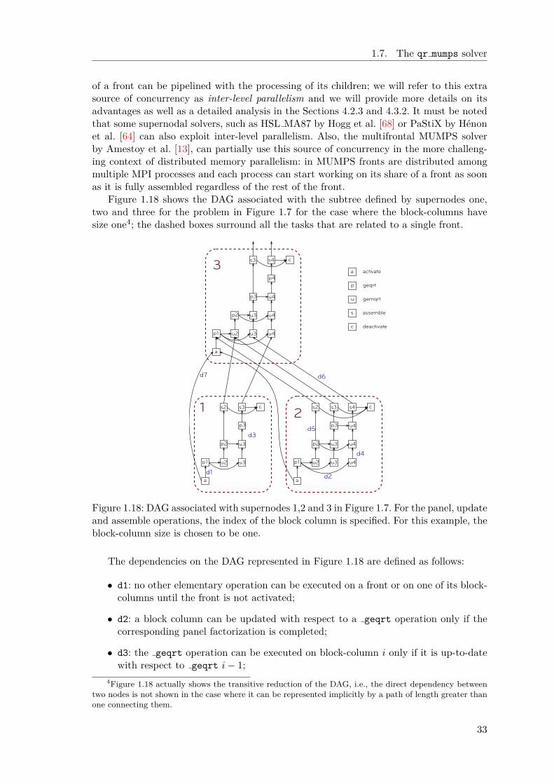
1.7. The qr mumps solver

of a front can be pipelined with the processing of its children; we will refer to this extrasource of concurrency as inter-level parallelism and we will provide more details on itsadvantages as well as a detailed analysis in the Sections 4.2.3 and 4.3.2. It must be notedthat some supernodal solvers, such as HSL MA87 by Hogg et al. [68] or PaStiX by Henonet al. [64] can also exploit inter-level parallelism. Also, the multifrontal MUMPS solverby Amestoy et al. [13], can partially use this source of concurrency in the more challeng-ing context of distributed memory parallelism: in MUMPS fronts are distributed amongmultiple MPI processes and each process can start working on its share of a front as soonas it is fully assembled regardless of the rest of the front.

Figure 1.18 shows the DAG associated with the subtree defined by supernodes one,two and three for the problem in Figure 1.7 for the case where the block-columns havesize one4; the dashed boxes surround all the tasks that are related to a single front.

12

a

p1 u2 u3

p2 u3

p3

s2 s3

a

p1 u2 u3

u3

u4

u4

u4

s2 s3 s4

p2

p3

cc

3

a

p1 u2 u3

u3

u4

u4

u4

p4

s3 s4

p2

p3

c

d1d2

d4

d5

d6d7

a

u

s

c

activate

p geqrt

gemqrt

assemble

deactivate

d3

Figure 1.18: DAG associated with supernodes 1,2 and 3 in Figure 1.7. For the panel, updateand assemble operations, the index of the block column is specified. For this example, theblock-column size is chosen to be one.

The dependencies on the DAG represented in Figure 1.18 are defined as follows:

• d1: no other elementary operation can be executed on a front or on one of its block-columns until the front is not activated;

• d2: a block column can be updated with respect to a geqrt operation only if thecorresponding panel factorization is completed;

• d3: the geqrt operation can be executed on block-column i only if it is up-to-datewith respect to geqrt i − 1;

4Figure 1.18 actually shows the transitive reduction of the DAG, i.e., the direct dependency betweentwo nodes is not shown in the case where it can be represented implicitly by a path of length greater thanone connecting them.

33

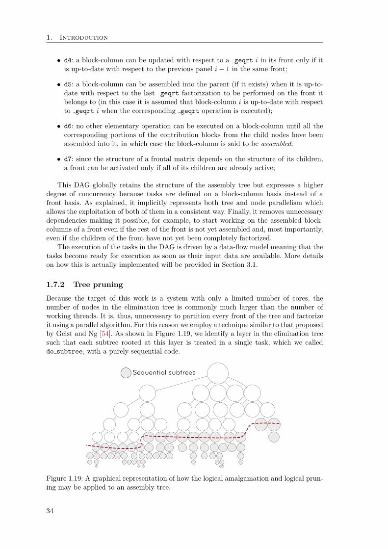
1. Introduction

• d4: a block-column can be updated with respect to a geqrt i in its front only if itis up-to-date with respect to the previous panel i − 1 in the same front;

• d5: a block-column can be assembled into the parent (if it exists) when it is up-to-date with respect to the last geqrt factorization to be performed on the front itbelongs to (in this case it is assumed that block-column i is up-to-date with respectto geqrt i when the corresponding geqrt operation is executed);

• d6: no other elementary operation can be executed on a block-column until all thecorresponding portions of the contribution blocks from the child nodes have beenassembled into it, in which case the block-column is said to be assembled;

• d7: since the structure of a frontal matrix depends on the structure of its children,a front can be activated only if all of its children are already active;

This DAG globally retains the structure of the assembly tree but expresses a higherdegree of concurrency because tasks are defined on a block-column basis instead of afront basis. As explained, it implicitly represents both tree and node parallelism whichallows the exploitation of both of them in a consistent way. Finally, it removes unnecessarydependencies making it possible, for example, to start working on the assembled block-columns of a front even if the rest of the front is not yet assembled and, most importantly,even if the children of the front have not yet been completely factorized.

The execution of the tasks in the DAG is driven by a data-flow model meaning that thetasks become ready for execution as soon as their input data are available. More detailson how this is actually implemented will be provided in Section 3.1.

1.7.2 Tree pruning

Because the target of this work is a system with only a limited number of cores, thenumber of nodes in the elimination tree is commonly much larger than the number ofworking threads. It is, thus, unnecessary to partition every front of the tree and factorizeit using a parallel algorithm. For this reason we employ a technique similar to that proposedby Geist and Ng [54]. As shown in Figure 1.19, we identify a layer in the elimination treesuch that each subtree rooted at this layer is treated in a single task, which we calleddo subtree, with a purely sequential code.

Figure 1.19: A graphical representation of how the logical amalgamation and logical prun-ing may be applied to an assembly tree.

34

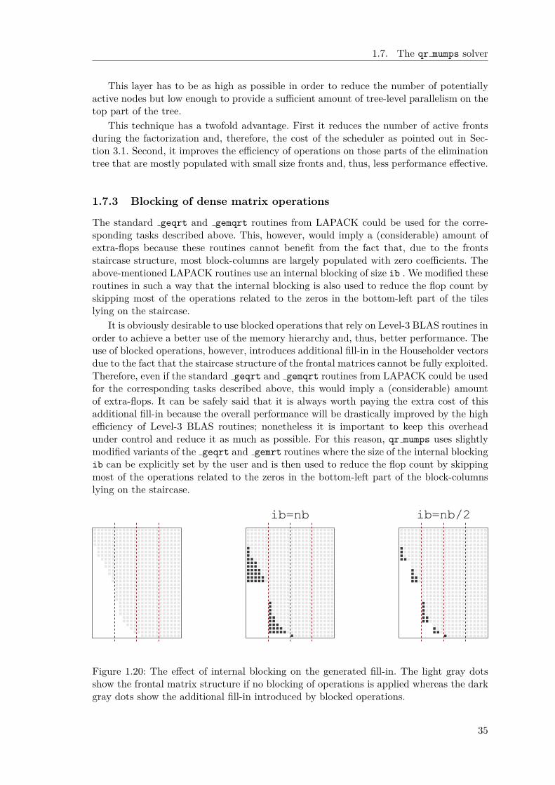
1.7. The qr mumps solver

This layer has to be as high as possible in order to reduce the number of potentiallyactive nodes but low enough to provide a sufficient amount of tree-level parallelism on thetop part of the tree.

This technique has a twofold advantage. First it reduces the number of active frontsduring the factorization and, therefore, the cost of the scheduler as pointed out in Sec-tion 3.1. Second, it improves the efficiency of operations on those parts of the eliminationtree that are mostly populated with small size fronts and, thus, less performance effective.

1.7.3 Blocking of dense matrix operations

The standard geqrt and gemqrt routines from LAPACK could be used for the corre-sponding tasks described above. This, however, would imply a (considerable) amount ofextra-flops because these routines cannot benefit from the fact that, due to the frontsstaircase structure, most block-columns are largely populated with zero coefficients. Theabove-mentioned LAPACK routines use an internal blocking of size ib . We modified theseroutines in such a way that the internal blocking is also used to reduce the flop count byskipping most of the operations related to the zeros in the bottom-left part of the tileslying on the staircase.

It is obviously desirable to use blocked operations that rely on Level-3 BLAS routines inorder to achieve a better use of the memory hierarchy and, thus, better performance. Theuse of blocked operations, however, introduces additional fill-in in the Householder vectorsdue to the fact that the staircase structure of the frontal matrices cannot be fully exploited.Therefore, even if the standard geqrt and gemqrt routines from LAPACK could be usedfor the corresponding tasks described above, this would imply a (considerable) amountof extra-flops. It can be safely said that it is always worth paying the extra cost of thisadditional fill-in because the overall performance will be drastically improved by the highefficiency of Level-3 BLAS routines; nonetheless it is important to keep this overheadunder control and reduce it as much as possible. For this reason, qr mumps uses slightlymodified variants of the geqrt and gemrt routines where the size of the internal blockingib can be explicitly set by the user and is then used to reduce the flop count by skippingmost of the operations related to the zeros in the bottom-left part of the block-columnslying on the staircase.

Figure 1.20: The effect of internal blocking on the generated fill-in. The light gray dotsshow the frontal matrix structure if no blocking of operations is applied whereas the darkgray dots show the additional fill-in introduced by blocked operations.

35

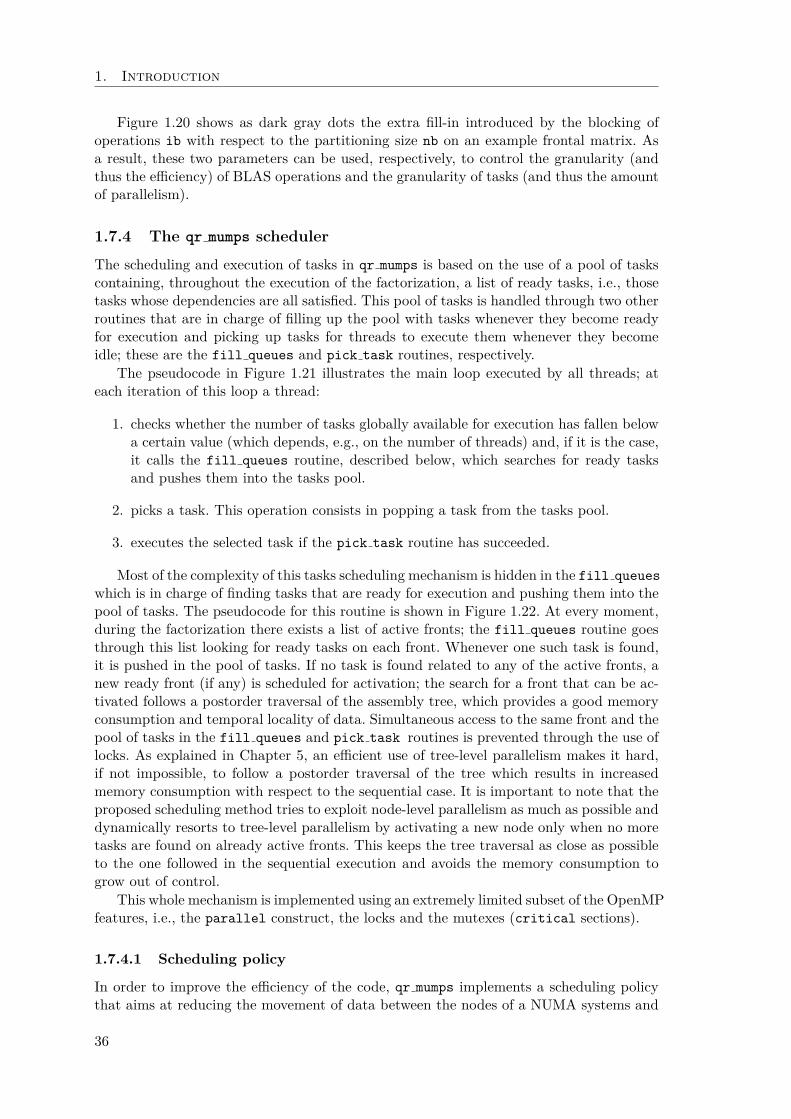
1. Introduction

Figure 1.20 shows as dark gray dots the extra fill-in introduced by the blocking ofoperations ib with respect to the partitioning size nb on an example frontal matrix. Asa result, these two parameters can be used, respectively, to control the granularity (andthus the efficiency) of BLAS operations and the granularity of tasks (and thus the amountof parallelism).

1.7.4 The qr mumps scheduler

The scheduling and execution of tasks in qr mumps is based on the use of a pool of taskscontaining, throughout the execution of the factorization, a list of ready tasks, i.e., thosetasks whose dependencies are all satisfied. This pool of tasks is handled through two otherroutines that are in charge of filling up the pool with tasks whenever they become readyfor execution and picking up tasks for threads to execute them whenever they becomeidle; these are the fill queues and pick task routines, respectively.

The pseudocode in Figure 1.21 illustrates the main loop executed by all threads; ateach iteration of this loop a thread:

1. checks whether the number of tasks globally available for execution has fallen belowa certain value (which depends, e.g., on the number of threads) and, if it is the case,it calls the fill queues routine, described below, which searches for ready tasksand pushes them into the tasks pool.

2. picks a task. This operation consists in popping a task from the tasks pool.

3. executes the selected task if the pick task routine has succeeded.

Most of the complexity of this tasks scheduling mechanism is hidden in the fill queues

which is in charge of finding tasks that are ready for execution and pushing them into thepool of tasks. The pseudocode for this routine is shown in Figure 1.22. At every moment,during the factorization there exists a list of active fronts; the fill queues routine goesthrough this list looking for ready tasks on each front. Whenever one such task is found,it is pushed in the pool of tasks. If no task is found related to any of the active fronts, anew ready front (if any) is scheduled for activation; the search for a front that can be ac-tivated follows a postorder traversal of the assembly tree, which provides a good memoryconsumption and temporal locality of data. Simultaneous access to the same front and thepool of tasks in the fill queues and pick task routines is prevented through the use oflocks. As explained in Chapter 5, an efficient use of tree-level parallelism makes it hard,if not impossible, to follow a postorder traversal of the tree which results in increasedmemory consumption with respect to the sequential case. It is important to note that theproposed scheduling method tries to exploit node-level parallelism as much as possible anddynamically resorts to tree-level parallelism by activating a new node only when no moretasks are found on already active fronts. This keeps the tree traversal as close as possibleto the one followed in the sequential execution and avoids the memory consumption togrow out of control.

This whole mechanism is implemented using an extremely limited subset of the OpenMPfeatures, i.e., the parallel construct, the locks and the mutexes (critical sections).

1.7.4.1 Scheduling policy

In order to improve the efficiency of the code, qr mumps implements a scheduling policythat aims at reducing the movement of data between the nodes of a NUMA systems and

36

1.7. The qr mumps solver

1 mainloop : do

if( n_ready_tasks < ntmin) then

3 ! if the number of threads falls

! below a certain value , fill -up

5 ! the queues

call fill_queues ()

7 end if

9 task = pick_task ()

11 select case(task%id)

case( geqrt)

13 call execute_geqrt ()

case( gemqrt )

15 call execute_gemqrt ()

case( assemble )

17 call execute_assemble ()

case( activate )

19 call execute_activate ()

case( deactivate )

21 call execute_deactivate ()

case( finish )

23 exit mainloop

end select

25 end do mainloop

Figure 1.21: main execution loop in qr mumps, executed by every thread.

1 found = .false.

forall (front in active fronts )

3 ! for each active front try to schedule

! ready tasks

5 found = found .or. push_geqrt (front)

found = found .or. push_gemqrt (front)

7 found = found .or. push_assemble (front)

found = found .or. push_deactivate (front)

9 end forall

11 if (found) then

! if tasks were pushed in the previous

13 ! loop return

return

15 else

! otherwise schedule the activation of

17 ! the next ready front

call push_activate (next ready front)

19 end if

21 if ( factorization over) call push_finish ()

Figure 1.22: fill queue routine in qr mumps, filling thread queues with tasks ready forexecution

37

1. Introduction

at reducing the time for traversing the DAG critical path which defines a lower bound onthe execution time of the task graph.

In the multifrontal method, Level-3 BLAS routines such as gemqrt operations repre-sent the largest share of computational cost. However there remain a significant amountof Level-2 BLAS routines as well as symbolic operations such as activate, assemble andgeqrt tasks whose efficiency is limited by the speed of memory. In particular many taskson the critical path are memory-bound and the impact of the time spent on this pathbecomes more and more important as the number of resources grows. In addition, somefrontal matrices, especially at the bottom of the tree, are too small to achieve asymptoticperformance on Level-3 routines. Therefore to achieve a good scalability of the multi-frontal factorization, it is important to execute these memory-bound kernels as efficientlyas possible. This can be done by executing the kernels on the threads which are the closestto the data they manipulate. For this purpose qr mumps introduces a concept of ownershipof a front: the thread that performs the activate operation on a front becomes its ownerand, therefore, becomes the privileged thread to perform all the subsequent tasks relatedto that front. This leads to a better performance of tasks because of the first-touch rulewhich is implemented in most (if not all) modern operating systems. The task pool is thenimplemented as a set of queues, one for each thread. In the fill queue routine, whena ready task is found, it is pushed in the queue associated with the thread that ownsthe related front. An activate task, instead, is pushed on the queue associated with thethread that executes the fill queues routine because the ownership of the related frontis not set yet. When a thread executes the pick task routine, it first looks for a readytask in its own queue. In the case where no task is available on the local queue, an archi-tecture aware work-stealing technique is employed, i.e., the thread will try to steal a taskfrom queues associated with threads with which it shares some level of memory (caches orDRAM module on a NUMA machine) and if still no task is found it will attempt to steal atask from any other queue. The computer’s architecture can be detected using tools suchas hwloc [30]. Experimental results presented by Buttari [32] show that this techniqueprovides some mild performance improvements.

In order to avoid any delay on the critical path that may increase the makespan andinduce resource starvation, tasks along this path are set with higher priorities over othertasks. In the case of a dense QR factorization with a 1D block-column partitioning it iseasy to see that panel operations lie on the critical path of the factorization task graph. Inqr mumps only two levels of priority can be used: although tasks are always popped fromthe head of each queue, they can be pushed either on the head or on the tail which allowsthe prioritisation of certain tasks. The panel operations for example are always pushed onthe head to prioritise them over other tasks.

1.8 Positioning of the thesis

Direct methods, introduced in Section 1.2, constitute a popular approach to find thesolution of large sparse linear systems of equations. They are often preferred for theirrobustness over other approaches like iterative methods whose efficiency largely dependson the numerical properties of the input problem. As presented in Section 1.3, in thecases of dense and sparse systems, recently developed factorization algorithms generate ahigh amount of concurrency and allow the exploitation of efficient kernels, yielding goodperformance on modern multicore architectures. The evolution of the hardware, however,with the increase in the number of cores per chips, the introduction of accelerators andthe diminishing amount of memory per core, face researchers with new challenges that we

38

1.8. Positioning of the thesis

tackle in this study: how to implement complex and irregular algorithms in an efficient yetportable way? how to make algorithms evolve and improve without being limited or con-strained by the complexity of their actual implementation? how to achieve the execution ofcomplex workloads on heterogeneous architectures equipped with multiple execution unitsrunning at different speeds and with memories having different capacities and speeds? Howto profile and analyze the performance of such codes on hybrid architectures?

This thesis attempts to address these issues through an approach which consists in rely-ing on the use of modern runtime systems in order to achieve a performance and memoryefficient yet portable implementation of the QR multifrontal method for heterogeneousarchitectures. Modern runtime systems, presented in Section 1.4.2, provide programminginterfaces complying with DAG-based algorithms that have recently become more andmore popular in the domain of linear algebra as explained for both the dense and sparsecase in Sections 1.5 and 1.6, respectively. The use of runtime systems has been largelystudied in the context of dense linear algebra but still represents a challenge for sparse al-gorithms such as the multifrontal method. The difficulty associated with the developmentof sparse methods on top of runtime systems lies in complexity of the DAG representingthe application with a large amount of tasks, with a great variety of kernels, granularityand memory consumption.

The first issue we address in Chapter 3 is to validate the pertinence of this approach byporting qr mumps to StarPU in a new version referred to as qrm starpu. We show that weachieve good performance with qrm starpu and provide a detailed performance analysiscomparing our new version with the original solver. In Chapter 4 we redesign the previousimplementation using a pure Sequential Task Flow model and improve our solver with theintegration of 2D, communication avoiding front factorization algorithms. Furthermore wedevelop a memory-aware algorithm allowing for controlling the memory consumption ofthe parallel multifrontal method. As we mention in Section 1.6, few sparse solvers are basedon runtime systems and none of them fully relies on these tools for handling parallelismand tasks execution, scheduling and data management. In our approach, we separate theexpression of algorithms from low-level details such as dependency management, datatransfer and data consistency that are delegated to the runtime system. In addition wetake advantage of the expressiveness of the programming models that we use to developnew features.

Exploiting heterogeneous systems is extremely challenging due to the complexity ofthese architectures. Current approaches presented in Section 1.6 generally rely on simplestatic scheduling strategies and some of the state-of-the-art solvers only exploit the accel-erator without taking advantage of the other resources on the architectures. In Chapter 6we address the data partitioning and scheduling issues that are critical to achieve perfor-mance on these architectures. We extend the 1D block-column partitioning used in theqr mumps solver (see Section 1.7) to a hierarchical block partitioning allowing to generateboth fine and coarse granularity tasks adapted to the processing unit capabilities. Weshow that the simplicity of the STF model facilitates the implementation of this datapartitioning with a complex dependency pattern and gives the ability to dynamically par-tition data. We develop a scheduling strategy capable of handling the task heterogeneityin the DAG and the diversity of resources on heterogeneous architectures. Thanks to themodular approach that we employ, the scheduler implemented in qrm starpu is genericand totally usable in other StarPU based applications.

The efficiency of the approaches presented above are assessed with a detailed perfor-mance analysis presented in Chapter 2. This performance analysis approach allows formeasuring and separately analysing several factors playing a role in performance and scal-ability such as locality issues and task pipelining. It should be noted this analysis requires

39

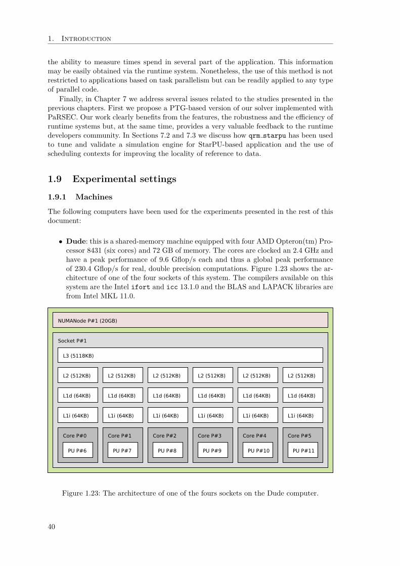
1. Introduction

the ability to measure times spend in several part of the application. This informationmay be easily obtained via the runtime system. Nonetheless, the use of this method is notrestricted to applications based on task parallelism but can be readily applied to any typeof parallel code.

Finally, in Chapter 7 we address several issues related to the studies presented in theprevious chapters. First we propose a PTG-based version of our solver implemented withPaRSEC. Our work clearly benefits from the features, the robustness and the efficiency ofruntime systems but, at the same time, provides a very valuable feedback to the runtimedevelopers community. In Sections 7.2 and 7.3 we discuss how qrm starpu has been usedto tune and validate a simulation engine for StarPU-based application and the use ofscheduling contexts for improving the locality of reference to data.

1.9 Experimental settings

1.9.1 Machines

The following computers have been used for the experiments presented in the rest of thisdocument:

• Dude: this is a shared-memory machine equipped with four AMD Opteron(tm) Pro-cessor 8431 (six cores) and 72 GB of memory. The cores are clocked an 2.4 GHz andhave a peak performance of 9.6 Gflop/s each and thus a global peak performanceof 230.4 Gflop/s for real, double precision computations. Figure 1.23 shows the ar-chitecture of one of the four sockets of this system. The compilers available on thissystem are the Intel ifort and icc 13.1.0 and the BLAS and LAPACK libraries arefrom Intel MKL 11.0.

NUMANode P#1 (20GB)

Socket P#1

L3 (5118KB)

L2 (512KB)

L1d (64KB)

L1i (64KB)

Core P#0

PU P#6

L2 (512KB)

L1d (64KB)

L1i (64KB)

Core P#1

PU P#7

L2 (512KB)

L1d (64KB)

L1i (64KB)

Core P#2

PU P#8

L2 (512KB)

L1d (64KB)

L1i (64KB)

Core P#3

PU P#9

L2 (512KB)

L1d (64KB)

L1i (64KB)

Core P#4

PU P#10

L2 (512KB)

L1d (64KB)

L1i (64KB)

Core P#5

PU P#11

Figure 1.23: The architecture of one of the fours sockets on the Dude computer.

40

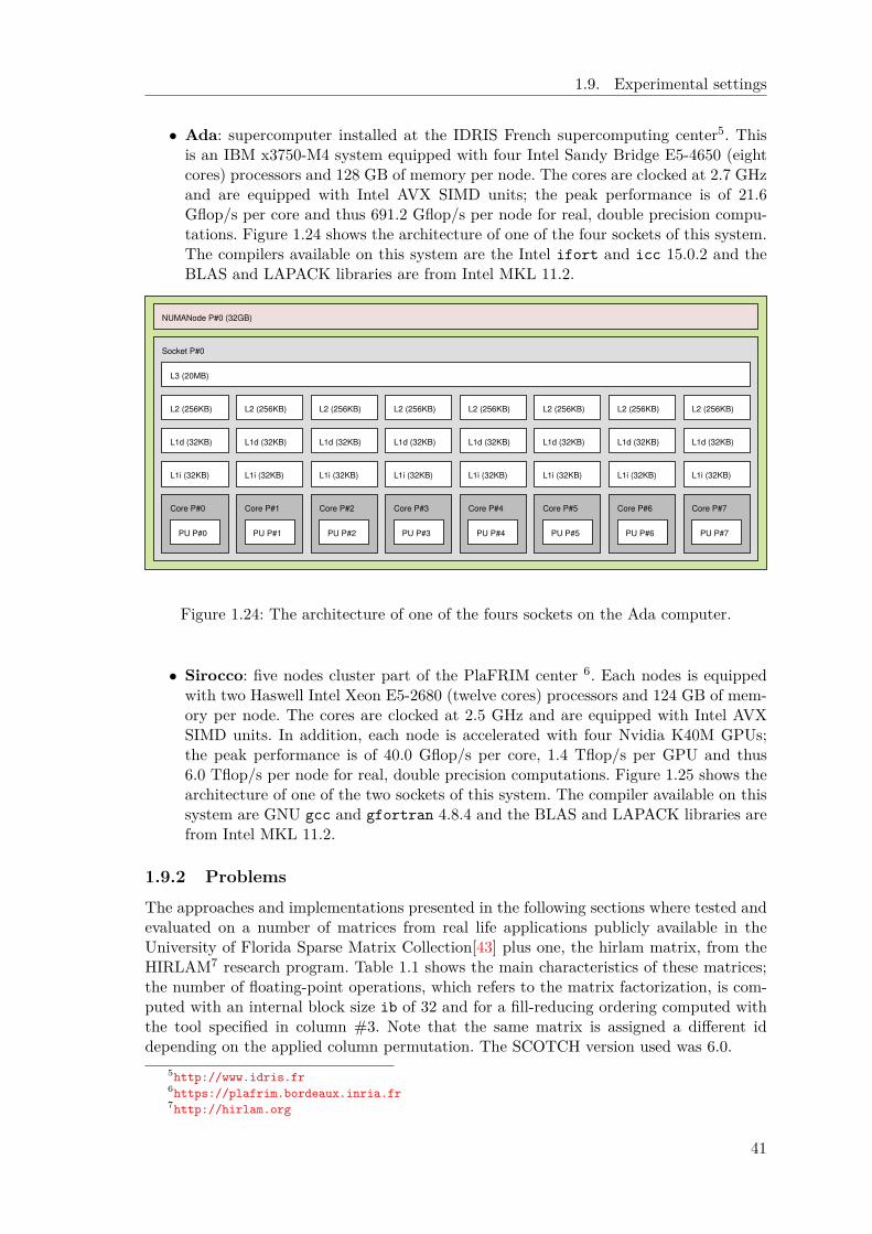
1.9. Experimental settings

• Ada: supercomputer installed at the IDRIS French supercomputing center5. Thisis an IBM x3750-M4 system equipped with four Intel Sandy Bridge E5-4650 (eightcores) processors and 128 GB of memory per node. The cores are clocked at 2.7 GHzand are equipped with Intel AVX SIMD units; the peak performance is of 21.6Gflop/s per core and thus 691.2 Gflop/s per node for real, double precision compu-tations. Figure 1.24 shows the architecture of one of the four sockets of this system.The compilers available on this system are the Intel ifort and icc 15.0.2 and theBLAS and LAPACK libraries are from Intel MKL 11.2.

NUMANode P#0 (32GB)

Socket P#0

L3 (20MB)

L2 (256KB)

L1d (32KB)

L1i (32KB)

Core P#0

PU P#0

L2 (256KB)

L1d (32KB)

L1i (32KB)

Core P#1

PU P#1

L2 (256KB)

L1d (32KB)

L1i (32KB)

Core P#2

PU P#2

L2 (256KB)

L1d (32KB)

L1i (32KB)

Core P#3

PU P#3

L2 (256KB)

L1d (32KB)

L1i (32KB)

Core P#4

PU P#4

L2 (256KB)

L1d (32KB)

L1i (32KB)

Core P#5

PU P#5

L2 (256KB)

L1d (32KB)

L1i (32KB)

Core P#6

PU P#6

L2 (256KB)

L1d (32KB)

L1i (32KB)

Core P#7

PU P#7

Figure 1.24: The architecture of one of the fours sockets on the Ada computer.

• Sirocco: five nodes cluster part of the PlaFRIM center 6. Each nodes is equippedwith two Haswell Intel Xeon E5-2680 (twelve cores) processors and 124 GB of mem-ory per node. The cores are clocked at 2.5 GHz and are equipped with Intel AVXSIMD units. In addition, each node is accelerated with four Nvidia K40M GPUs;the peak performance is of 40.0 Gflop/s per core, 1.4 Tflop/s per GPU and thus6.0 Tflop/s per node for real, double precision computations. Figure 1.25 shows thearchitecture of one of the two sockets of this system. The compiler available on thissystem are GNU gcc and gfortran 4.8.4 and the BLAS and LAPACK libraries arefrom Intel MKL 11.2.

1.9.2 Problems

The approaches and implementations presented in the following sections where tested andevaluated on a number of matrices from real life applications publicly available in theUniversity of Florida Sparse Matrix Collection[43] plus one, the hirlam matrix, from theHIRLAM7 research program. Table 1.1 shows the main characteristics of these matrices;the number of floating-point operations, which refers to the matrix factorization, is com-puted with an internal block size ib of 32 and for a fill-reducing ordering computed withthe tool specified in column #3. Note that the same matrix is assigned a different iddepending on the applied column permutation. The SCOTCH version used was 6.0.

5http://www.idris.fr6https://plafrim.bordeaux.inria.fr7http://hirlam.org

41

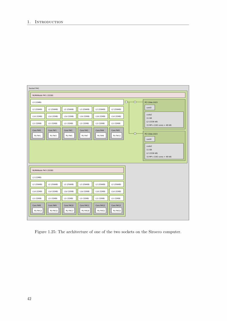
1. Introduction

Socket P#1

NUMANode P#1 (32GB)

L3 (15MB)

L2 (256KB)

L1d (32KB)

L1i (32KB)

Core P#0

PU P#1

L2 (256KB)

L1d (32KB)

L1i (32KB)

Core P#1

PU P#3

L2 (256KB)

L1d (32KB)

L1i (32KB)

Core P#2

PU P#5

L2 (256KB)

L1d (32KB)

L1i (32KB)

Core P#3

PU P#7

L2 (256KB)

L1d (32KB)

L1i (32KB)

Core P#4

PU P#9

L2 (256KB)

L1d (32KB)

L1i (32KB)

Core P#5

PU P#11

PCI 10de:1023

card3

cuda2

11 GB

L2 (1536 kB)

15 MP x (192 cores + 48 kB)

PCI 10de:1023

card4

cuda3

11 GB

L2 (1536 kB)

15 MP x (192 cores + 48 kB)

NUMANode P#3 (32GB)

L3 (15MB)

L2 (256KB)

L1d (32KB)

L1i (32KB)

Core P#8

PU P#13

L2 (256KB)

L1d (32KB)

L1i (32KB)

Core P#9

PU P#15

L2 (256KB)

L1d (32KB)

L1i (32KB)

Core P#10

PU P#17

L2 (256KB)

L1d (32KB)

L1i (32KB)

Core P#11

PU P#19

L2 (256KB)

L1d (32KB)

L1i (32KB)

Core P#12

PU P#21

L2 (256KB)

L1d (32KB)

L1i (32KB)

Core P#13

PU P#23

Figure 1.25: The architecture of one of the two sockets on the Sirocco computer.

42

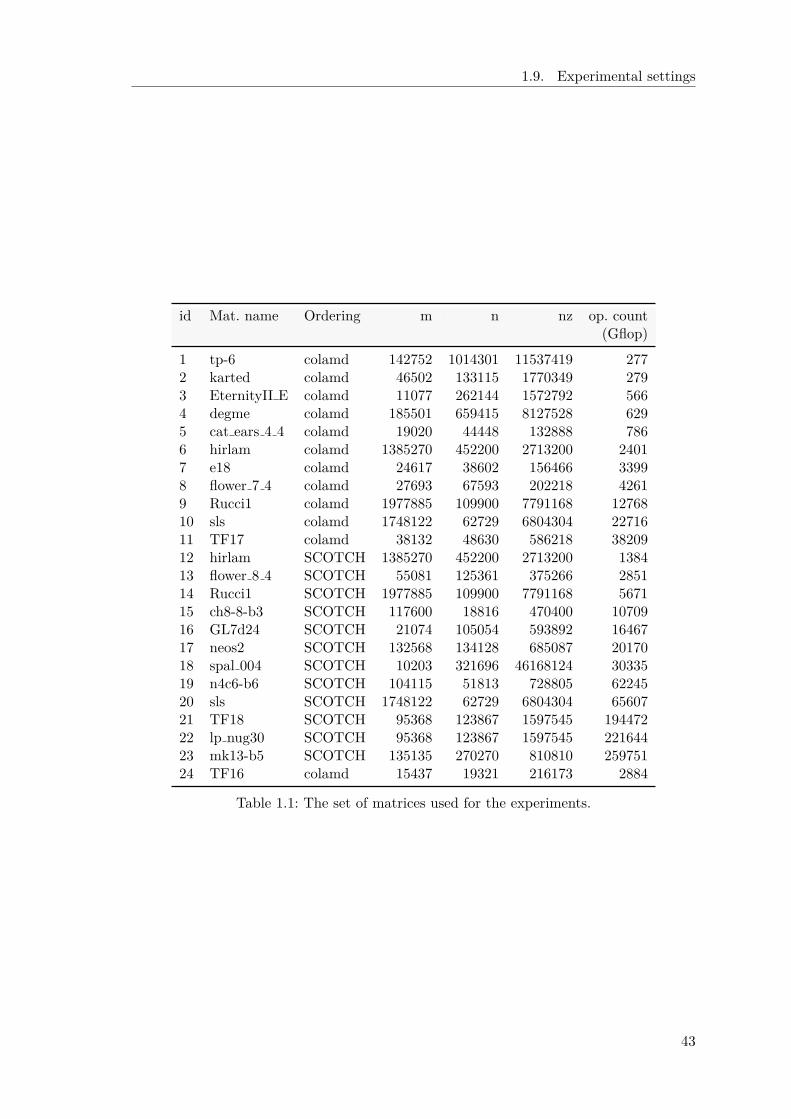
1.9. Experimental settings

id Mat. name Ordering m n nz op. count(Gflop)

1 tp-6 colamd 142752 1014301 11537419 2772 karted colamd 46502 133115 1770349 2793 EternityII E colamd 11077 262144 1572792 5664 degme colamd 185501 659415 8127528 6295 cat ears 4 4 colamd 19020 44448 132888 7866 hirlam colamd 1385270 452200 2713200 24017 e18 colamd 24617 38602 156466 33998 flower 7 4 colamd 27693 67593 202218 42619 Rucci1 colamd 1977885 109900 7791168 1276810 sls colamd 1748122 62729 6804304 2271611 TF17 colamd 38132 48630 586218 3820912 hirlam SCOTCH 1385270 452200 2713200 138413 flower 8 4 SCOTCH 55081 125361 375266 285114 Rucci1 SCOTCH 1977885 109900 7791168 567115 ch8-8-b3 SCOTCH 117600 18816 470400 1070916 GL7d24 SCOTCH 21074 105054 593892 1646717 neos2 SCOTCH 132568 134128 685087 2017018 spal 004 SCOTCH 10203 321696 46168124 3033519 n4c6-b6 SCOTCH 104115 51813 728805 6224520 sls SCOTCH 1748122 62729 6804304 6560721 TF18 SCOTCH 95368 123867 1597545 19447222 lp nug30 SCOTCH 95368 123867 1597545 22164423 mk13-b5 SCOTCH 135135 270270 810810 25975124 TF16 colamd 15437 19321 216173 2884

Table 1.1: The set of matrices used for the experiments.

43

Chapter 2

Performance analysis approach

Performance profiling and analysis is one of the cornerstones of High Performance Com-puting. Nonetheless, it may be a challenging task to achieve, especially in the case ofcomplex applications or algorithms and large or complex architectures. Therefore, it is nosurprise that performance profiling has been the object of a very vast amount of literature.

In the case of sequential applications, a rather simple but effective approach consistsin computing the efficiency of the code as a ratio of the attained speed and a referenceperformance which depends on the peak capability of the underlying architecture. Becauseprocessing units and memories work at different speeds, this reference performance variesdepending on whether the application is compute bound (i.e., limited by the speed ofthe processing unit) or memory bound and to what extent. The Roofline model [115]is a popular method for computing this performance upper bound as a function of theoperational intensity:

AttainableGflop/s

= min

{Peak Floating-point

Performance,Peak MemoryBandwidth

×Operationalintensity

}.

The peak floating-point performance and peak memory bandwidth can be set equal tothe theoretical values of the architecture; these values, however, are commonly unattain-able and therefore these parameter values are computed using benchmarks like the BLASgemm (matrix-matrix multiply) operation, which is commonly considered as the fastestcompute-bound operation, or the STREAM [88] benchmark, respectively. The rooflinemodel can also be used for shared-memory, parallel applications but cannot be extendedto the case where accelerators are used or to distributed-memory, parallel codes. Moreover,its use is difficult in the case of complex applications, such as the multifrontal method,which include both memory and compute-bound operations whose relative weight variesdepending on the input problem.

The performance of a parallel code, either shared or distributed-memory, on a homo-geneous platform (i.e., where all the processing units are the same) is commonly assessedmeasuring its speedup, i.e., the ratio between the sequential and the parallel executiontimes t(1)/t(p), or, equivalently, the parallel efficiency

e(p) =t(1)

t(p) × p

where p is the number of processing units used. The scalability measures the ability ofa parallel code to reduce the execution time as more resources are provided. Amadahl’slaw can be used to define a bound on the achievable speedup (or parallel efficiency or

45

2. Performance analysis approach

scaling) of a parallel code but, again, this is very hard to achieve for complex and irregularapplications.

The emerging heterogeneous architectures represent a challenge for the performanceevaluation of parallel algorithms compared to the uni-processor and parallel, homogeneousenvironments. Accelerators, not only process data at different speeds compared to theCPUs but also have different capabilities, i.e., are more or less suited to different typesof operations, and are attached to their own memory which has different latency andbandwidth than that on the host. The performance analysis of codes that use acceleratorsis often limited to measuring the added performance brought by the accelerators, that is,a simple speed comparison with the CPU-only execution.

Although the above presented techniques can be used to achieve a rough evaluation ofthe performance of a parallel code, none of them provides any insight which can guide theHPC expert in reformulating or improving his algorithms or the programmer in optimizinghis code in order to achieve better performance. Many factors play an important role inthe performance and scalability of a code; among the others, we can mention the cost ofdata transfers and synchronizations, the granularity of operations, the properties of thealgorithm and the amount of concurrency it can deliver. A quantitative evaluation of thesefactors can be extremely valuable.

In order to evaluate the effectiveness of the techniques proposed in Chapters 3, 4 and 6as well as of the software that implements them, we developed a novel performance analysisapproach [S1, C2]. First, we introduce a method for computing a relatively tight upperbound for the performance attainable by the parallel code, which is not merely a sumof the peak performance of the available processing units; this performance reference iscomputed by not only taking into account the features of the underlying architecture, butalso the properties of the implemented algorithm and allows for evaluating the efficiencyof a parallel code. Then we show how it is possible to factorize this efficiency measureinto a product of terms that allow for assessing, singularly, the effect of several factorsplaying a role in the performance and scalability of a code. This analysis requires theability to retrieve specific information from the execution that are easy to gather whenusing a runtime system.

2.1 General analysis

Consider the problem of evaluating the execution of a parallel application on a targetcomputing environment composed of p heterogeneous processors such as CPUs and GPUsworkers. Critical factors playing a role on parallel executions must be considered to com-pute realistic performance bounds and understand to what extent each of these factorsmay limit the performance. Idle times and data transfers (communications, in general) forexample represent a major bottleneck for performance of parallel executions. Also we seekto quantify the cost of the runtime system, if any, compared to the workload in order toevaluate the effectiveness of these tools and estimate the overhead they induce.

In the proposed performance evaluation approach we perform a detailed analysis ofthe execution times by considering the cumulative times spent by all threads in the mainphases of the execution:

• tt(p): The time spent in tasks which represent the workload of the application;

• tr(p): The time spent in the runtime for handling the execution of the application(in our case, this includes building the DAG and scheduling the tasks);

46

2.1. General analysis

• tc(p): The time spent performing communications that are not overlapped by com-putations. This corresponds to the time spent by workers waiting for data to betransferred on their associated memory node before being able to execute a task;

• ti(p): The idle time spent waiting for dependencies between tasks to be satisfied.

The execution time of the factorization t(p), may be expressed, using these cumulativetimes, as follows:

t(p) =tt(p) + tr(p) + tc(p) + ti(p)

p

The efficiency of a parallel code can be defined as

e(p) =tmin(p)

t(p)

where tmin(p) is a lower bound on the execution time with p processes. A possible wayof computing tmin(p) for a task graph is to measure the execution time associated withthe optimal schedule. However, given the complexity of the task scheduling problem in thegeneral case it is not reasonable to compute this tmin(p) for any input problem. Insteadwe choose to use a looser bound that consists in computing the optimal value of tmin(p)for a relaxed version of the initial scheduling problem built on the following assumptions:

1. There are no dependencies between tasks which means that we consider an embar-rassingly parallel problem, i.e., ti(p) = 0;

2. The runtime does not induce any overhead on the execution time, i.e., tr(p) = 0;

3. The cost of all data transfers is equal to zero, i.e., tc(p) = 0;

4. Tasks are moldable meaning that they may be processed by multiple processors.

In order to compute tmin(p) we introduce the following notation: for a set of tasks Ωrunning on a set of p resources denoted by R, we define αω

r as the share of work in taskω processed by resource r and tω

r as the time spent by resource r processing its share oftask ω. Then tmin(p) can be computed as the solution of the following linear program:

Linear Program 1Minimize T such that, for all r ∈ R and for all ω ∈ Ω:

∑ω∈Ω

αωr tω

r = tr ≤ T

|R|∑r=1

αωr = 1

where the tωr can be computed using a performance model. Note that the problem of

finding tmin(p) is equivalent to minimizing the area αωr tω

r for all ω ∈ Ω and r ∈ R. For thisreason the optimal value tmin(p) is replaced by tarea(p) in the following. We illustrate howtarea(p) is defined in Figure 2.1 on a simple execution with three resources. On the left ofthe figure is represented the trace of the real execution where t(p) is measured. On theright is represented the optimal schedule for the relaxed version of the original schedulingproblem where tarea(p) is measured.

Note that parallelism is normally achieved by partitioning operations and data; this im-plies a smaller granularity of tasks and thus, likely, a poorer performance of the operations

47

2. Performance analysis approach

PU2

PU1

PU0

(a) Actual schedule.

PU2

PU1

PU0area

(b) Area schedule.

Figure 2.1: Illustration on a simple Gantt chart of a parallel execution with three workers.

performed by them. Moreover, parallel algorithms often trade floating-point operations forconcurrency and therefore may perform more operations than the corresponding sequen-tial ones (this is, for example, the case of 2D communication avoiding QR factorizations,as explained in Section 1.3.1). Based on these observations, we can further refine the effi-ciency definition above replacing tarea(p) with tarea(p) computed as the solution of LinearProgram 1 assuming ω ∈ Ω, where Ω is the set of tasks of the sequential algorithm. Inother words, in tarea(p) we assume that there is no performance loss when working onpartitioned data and that the parallel algorithm has the same cost as the sequential one.Please note that this also models the fact that in some cases data are inherently of smallgranularity and, therefore, tasks that work on them have a poor performance regardlessof the partitioning.

By replacing the term t(p) in the expression of the parallel efficiency using cumulativetimes and noting that tarea

t (p) = p × tarea(p) from the definition of our lower bound, wemay express the parallel efficiency as as

e(p) =tarea(p)

t(p)=

tarea(p) × p

tt(p) + tr(p) + tc(p) + ti(p)=

tareat (p)

tt(p) + tr(p) + tc(p) + ti(p)

=

eg

tareat (p)

tareat (p)

·

et

tareat (p)

tt(p)·

er

tt(p)

tt(p) + tr(p)·

ec

tt(p) + tr(p)

tt(p) + tr(p) + tc(p)·

ep

tt(p) + tr(p) + tc(p)

tt(p) + tr(p) + tc(p) + ti(p).

This expression allows us to decompose the parallel efficiency as the product of fivewell identified effects:

• eg: the granularity efficiency, which measures how the overall efficiency is reducedby the data partitioning and the use of parallel algorithms. This loss of efficiencyis mainly due to the fact that because of the partitioning of data into fine grainedblocks, elementary operations do not run at the same speed as in the purely sequen-tial code and also to the fact that the parallel algorithm may perform more flopsthan the sequential one;

• et: the task efficiency, measures how well the assignment of tasks to processingunits matches the tasks properties to the units capabilities as well as the exploitationof data locality (more details are provided below);

• er: the runtime efficiency, which measures the cost of the runtime system withrespect to the actual work done;

• ec: the communication efficiency, which measures the cost of communicationswith respect to the actual work done due to data transfers between workers;

48

2.1. General analysis

• ep: the pipeline efficiency, which measures how well the tasks have been pipelined.This includes two effects. First, the quality of the scheduling because if the schedulingpolicy takes bad decisions (for example, it delays the execution of tasks along thecritical path) many stalls can be introduced in the pipeline. Second, the shape ofthe DAG or, more generally, the amount of concurrency it delivers: for example, inthe extreme case where the DAG is a chain of tasks, any scheduling policy will doas bad because all the workers except one will be idling at any time.

Analysis for homogeneous multicore systems In the case of an homogeneous archi-tecture such as a multicore system with p cores, the solution of Linear Program 1 greatlysimplifies and can be easily found.

tarea(p) and tarea(p) do not have to be computed but can be measured by timing,respectively, the sequential execution of the sequential algorithm and the sequential exe-cution of the parallel algorithm (with the corresponding data partitioning), that is

tarea(p) =t(1)

p, tarea(p) =

t(1)

p. (2.1)

Note that in a sequential execution the cost of the communications and of the runtimeas well as the idle times are all identically equal to zero and therefore t(1) = tt(1) andt(1) = tt(1).

Replacing t(p) and tarea(p) in the expression of the parallel efficiency using the cumu-lative times we obtain:

e(p) =tt(1)

tt(p) + tr(p) + ti(p)

=

eg

tt(1)

tt(1)·

et

tt(1)

tt(p)·

er

tt(p)

tt(p) + tr(p) + tc(p)·

ep

tt(p) + tr(p)

tt(p) + tr(p) + ti(p).

Here we assumed ec = 1 because there are no explicit or measurable data transfers.These, however, happen implicitly when tasks access data which are remotely located inthe NUMA memory system; this makes the tasks execution time tt(p) increase as thenumber of cores p increases. This effect is measured by et.

Analysis for heterogeneous systems Compared to the homogeneous case, computingtarea(p) and tarea(p) in the context of heterogeneous systems is more complex because taskexecution times depend on the type of resources where they are executed. Therefore weneed need to solve the Linear Program in 1 to determine these values. The first stepconsists in gathering the execution times for every task on every possible computationalunit. Then the linear system is built either statically if all tasks are known in advanceor by registering it during an actual execution and finally solved using a linear programsolver.

The tasks efficiency, in this case, still measures the effect of implicit communicationsbut also, and more importantly, how well the heterogeneity of the processing units isexploited. In other words, et measures how well tasks have been mapped to computationalunits with respect to the optimal mapping computed by solving the linear program. Notethat this efficiency is not necessarily lower than one and it is closely related to the pipelineefficiency:

49

2. Performance analysis approach

• et < 1: tasks are globally being executed at a lower speed with respect to the optimal.This may happen because the tasks assigned to the different processing units are notof the good type; this is, for example, the case where very small granularity tasksare executed by GPUs;

• et > 1: note that a particularly naive scheduling policy can map all the tasks to fasterunits. This would obviously result in a small cumulative tasks execution time tt(p)but would inevitably lead to the starvation of the slower units and, as a consequence,to a poor pipeline efficiency ep.

As a result, the quality of the scheduling policy can be measured by the product ofthe tasks and pipeline efficiencies et · ep which is always less than one.

2.2 Discussion

As discussed in the previous section, the pipeline efficiency ep may be lowered eitherbecause of a lack of parallelism in the DAG or as a result of bad scheduling decisionstaken during the execution. The distinction between the two phenomena can be madequalitatively by looking at the execution traces but the analysis is basic and inaccurate.

Section 4.2.3. The analysis of the critical path defined as the longest path in the theDAG of tasks allows to decide what is the limiting factor for the pipeline efficiency. Ifwe note CP the set of tasks on the critical path (longest path from an entry task to anexit task) of the DAG and Lω the workload associated with the task ω, the maximumachievable speedup is the following:

S∞ =

∑ω∈Ω Lω∑

ω∈CP Lω

This quantity gives the maximal amount of parallelism available in a DAG, and givena multicore architecture, one can expect to have at most the speedup given by its valuecompared to a sequential execution. In practice, the actual speedup would be much lowerbecause of the aforementioned effects such as granularity efficiency and locality efficiency.Therefore, when targeting an architecture such as a multicore machine with p cores, a lowvalue S∞ (lower than p for example) indicates that the DAG is not suited and will notdeliver enough parallelism to feed all the resources.

In a heterogeneous context the formulation of S∞ becomes more complex as there is nolonger equivalence between the length of a task and its execution time. For this reason thecritical path may not be interpreted as the longest path in the DAG in terms of work load.In an effort to adapt the definition of S∞ to heterogeneous architecture it is possible toreformulate it by replacing the length of the critical path with a lower bound on its length.For example we define CPmin as the critical path of a DAG, considering the minimumcomputational cost. Using the previous notations the minimal computational cost of atask ω on every resources may be expressed as minr∈R tω

r . Then we use this notion toderive another definition of S∞ as follows:

S∞ =

∑ω∈Ω minr∈R tω

r∑ω∈CPmin

minr∈R tωr

The previous definition of S∞ for homogeneous architectures may be seen as a partic-ular case of this definition. Note that the denominator in the latter formula does not equalthe length of the critical path because it does not take into account the communicationcost between processors. In addition as we will see later the definition of a critical path is

50

2.2. Discussion

not trivial in an heterogeneous context as it is associated with a choice of metric for thecomputational cost of a task that can have several interpretations. For instance the criticalpath may be determined by considering the average computation cost of tasks denoted tω.

The second metric we use to evaluate the execution time t(p), commonly referredto as makespan, is the ratio between this value and the length of the critical path whoseexpression is straightforward in a homogeneous case and can be interpreted as the efficiencyof the makespan:

emakepan(p) =t(p)∑

ω∈CP tω

As for the definition of our previous metric this formula may not be easily generalizedto a heterogeneous context. Using the same methodology as previously we simply replacethe expression of the critical path by a lower bound on the length of the critical paththerefore corresponding to a lower bound on the makespan ensuring that this quantity isinferior to one.

Another idea to take into account the critical path in the case of a parallel hetero-geneous execution, suggested by Agullo et al. [6], is to integrate a constraint in LinearProgram 1 corresponding to the lower bound on the length of the critical path that weuse in the previous metrics S∞ and emakepan(p). With this constraint, we express the factthat the makespan may not be larger than this lower bound:

∑ω∈CPmin

minr∈R

tωr ≤ T

However in the general case the number of variables is important (one variable pertask) and increases with the size of the problem which makes the linear program hard tosolve without constraints and consequently even harder when adding a constraint. Agulloet al. [6] show that given a problem (Cholesky factorization in their case) it is possible toreduce the linear program to another one of small size and whose size is independent fromthe problem. This is made possible by the regularity of dense linear algebra algorithm thatthey tackle. It may be noted that in our study it is not possible to make any assumptionson the regularity our problems.

To handle the complexity of complex DAGs arising in the case of sparse linear algebrait is possible to evaluate the impact of scheduling algorithm and communication usingsimulations. As presented by Agullo et al. [6] and Stanisic et al. [108] in the case ofdense algorithms and as we show in Chapter 7.2 in the context of qr mumps for sparseproblems, with the help of tools that may be integrated in runtime systems such as StarPU-SimGrid it is possible to reproduce execution of a DAG on a parallel machine. In additionsome parameters may be changed such as bandwidths and tasks processing speeds (inorder to remove the effect of locality for example) in order to measure the influence ofthese parameters on the execution time and evaluate the behavior of scheduling strategiesunder some circumstances (for example when the number of processors grows) withoutperforming the actual execution.

51

Chapter 3

Task-based multifrontal method:porting on a general purposeruntime system

The task-based multifrontal QR method implemented in qr mumps and presented in Sec-tion 1.7 constitutes an extremely irregular workload, with tasks of different granularitiesand characteristics and with variable memory consumption. In the qr mumps solver, thetasks that form this workload are scheduled through a hand-written code which relies onthe knowledge of the algorithm. In this chapter we will first comment on the shortcomingsof the scheduling method implemented in the qr mumps solver described in Section 1.7.We will then focus on the porting of the qr mumps algorithm on top of a general purposeruntime system in order to asses the usability of these tools on such large and complexworkloads [C1]. As explained, modern runtime systems provide programming interfacesthat comply with a DAG-based programming paradigm and powerful engines for schedul-ing the tasks into which the application is decomposed. For these reason, these tools arevery well suited for qr mumps; nonetheless, this porting is not straightforward and requiressome care. The result of this work is a preliminary version of a new code which we refer toas qrm starpu. This code will be used to run the experiments presented in Section 3.2.3that show how this migration to a general purpose runtime system leads to a much moremodular and portable code at the cost of a negligible loss of performance.

3.1 Efficiency and scalability of the qr mumps scheduler

A consequence of the design of the qr mumps scheduler presented in Section 1.7.4 is thatthe size of the search space for the fill queues routine is proportional to the number ofactive fronts, at a given moment, during the factorization. The size of this search space,however, can grow excessively large and, consequently, the cost of the fill queues routinemay become unbearable. This is the case for example when the the elimination tree iscomposed of a large number of nodes. Moreover, when the number working threads growswe observe the following two effects: first the layer computed for the logical tree pruning(see Section 1.7.2) in the elimination tree tends to go down the tree which increases thenumber of frontal matrices to be activated during the factorization; Second the numberof resources to feed the scheduler becomes higher and the activation of frontal matricesis triggered sooner during the factorization. In particular, nothing prevents the schedulerfrom activating all the frontal matrices as soon as they are ready which can make thesearch space arbitrarily large. Two different techniques were presented by Buttari [32] to

53

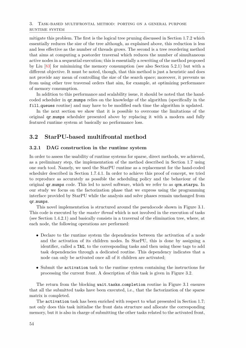
3. Task-based multifrontal method: porting on a general purpose

runtime system

mitigate this problem. The first is the logical tree pruning discussed in Section 1.7.2 whichessentially reduces the size of the tree although, as explained above, this reduction is lessand less effective as the number of threads grows. The second is a tree reordering methodthat aims at computing a postorder traversal which reduces the number of simultaneousactive nodes in a sequential execution; this is essentially a rewriting of the method proposedby Liu [83] for minimizing the memory consumption (see also Section 5.2.1) but with adifferent objective. It must be noted, though, that this method is just a heuristic and doesnot provide any mean of controlling the size of the search space; moreover, it prevents usfrom using other tree traversal orders that aim, for example, at optimizing performanceof memory consumption.

In addition to this performance and scalability issue, it should be noted that the hand-coded scheduler in qr mumps relies on the knowledge of the algorithm (specifically in thefill queues routine) and may have to be modified each time the algorithm is updated.

In the next section we show that it is possible to overcome the limitations of theoriginal qr mumps scheduler presented above by replacing it with a modern and fullyfeatured runtime system at basically no performance loss.

3.2 StarPU-based multifrontal method

3.2.1 DAG construction in the runtime system

In order to assess the usability of runtime systems for sparse, direct methods, we achieved,as a preliminary step, the implementation of the method described in Section 1.7 usingone such tool. Namely, we used the StarPU runtime as a replacement for the hand-codedscheduler described in Section 1.7.4.1. In order to achieve this proof of concept, we triedto reproduce as accurately as possible the scheduling policy and the behaviour of theoriginal qr mumps code. This led to novel software, which we refer to as qrm starpu. Inour study we focus on the factorization phase that we express using the programminginterface provided by StarPU while the analysis and solve phases remain unchanged fromqr mumps.

This novel implementation is structured around the pseudocode shown in Figure 3.1.This code is executed by the master thread which is not involved in the execution of tasks(see Section 1.4.2.1) and basically consists in a traversal of the elimination tree, where, ateach node, the following operations are performed:

• Declare to the runtime system the dependencies between the activation of a nodeand the activation of its children nodes. In StarPU, this is done by assigning aidentifier, called a TAG, to the corresponding tasks and then using these tags to addtask dependencies through a dedicated routine. This dependency indicates that anode can only be activated once all of it children are activated;

• Submit the activation task to the runtime system containing the instructions forprocessing the current front. A description of this task is given in Figure 3.2.

The return from the blocking wait tasks completion routine in Figure 3.1 ensuresthat all the submitted tasks have been executed, i.e., that the factorization of the sparsematrix is completed.

The activation task has been enriched with respect to what presented in Section 1.7;not only does this task initialise the front data structure and allocate the correspondingmemory, but it is also in charge of submitting the other tasks related to the activated front,

54

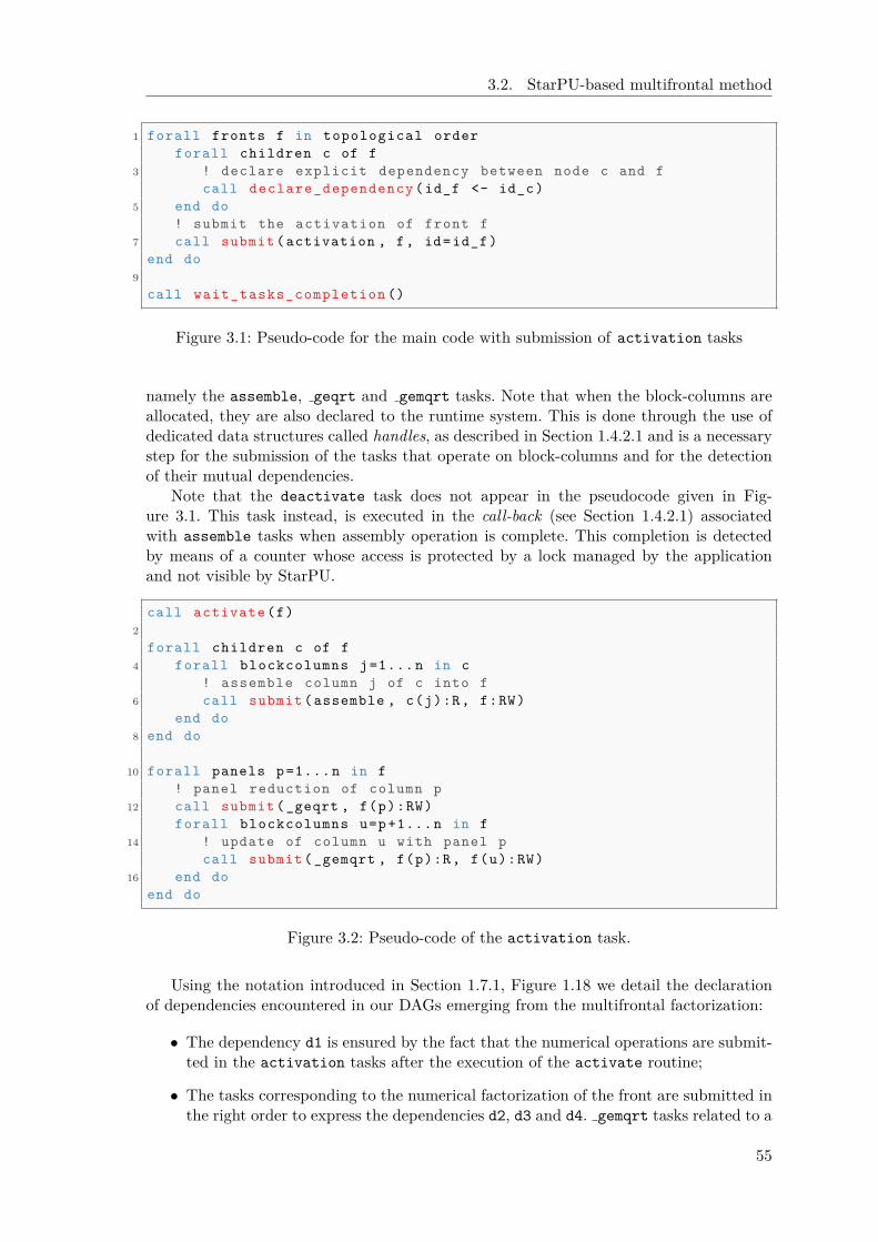
3.2. StarPU-based multifrontal method

1 forall fronts f in topological order

forall children c of f

3 ! declare explicit dependency between node c and f

call declare_dependency (id_f <- id_c)

5 end do

! submit the activation of front f

7 call submit (activation , f, id=id_f)

end do

9

call wait_tasks_completion ()

Figure 3.1: Pseudo-code for the main code with submission of activation tasks

namely the assemble, geqrt and gemqrt tasks. Note that when the block-columns areallocated, they are also declared to the runtime system. This is done through the use ofdedicated data structures called handles, as described in Section 1.4.2.1 and is a necessarystep for the submission of the tasks that operate on block-columns and for the detectionof their mutual dependencies.

Note that the deactivate task does not appear in the pseudocode given in Fig-ure 3.1. This task instead, is executed in the call-back (see Section 1.4.2.1) associatedwith assemble tasks when assembly operation is complete. This completion is detectedby means of a counter whose access is protected by a lock managed by the applicationand not visible by StarPU.

call activate (f)

2

forall children c of f

4 forall blockcolumns j=1...n in c

! assemble column j of c into f

6 call submit (assemble , c(j):R, f:RW)

end do

8 end do

10 forall panels p=1...n in f

! panel reduction of column p

12 call submit (_geqrt , f(p):RW)

forall blockcolumns u=p+1...n in f

14 ! update of column u with panel p

call submit (_gemqrt , f(p):R, f(u):RW)

16 end do

end do

Figure 3.2: Pseudo-code of the activation task.

Using the notation introduced in Section 1.7.1, Figure 1.18 we detail the declarationof dependencies encountered in our DAGs emerging from the multifrontal factorization:

• The dependency d1 is ensured by the fact that the numerical operations are submit-ted in the activation tasks after the execution of the activate routine;

• The tasks corresponding to the numerical factorization of the front are submitted inthe right order to express the dependencies d2, d3 and d4. gemqrt tasks related to a

55

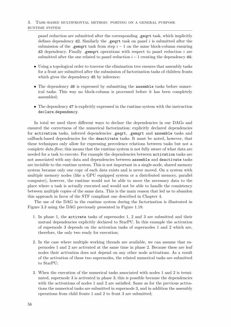
3. Task-based multifrontal method: porting on a general purpose

runtime system

panel reduction are submitted after the corresponding geqrt task, which implicitlydefines dependency d2. Similarly the geqrt task on panel i is submitted after thesubmission of the gemqrt task from step i − 1 on the same block-column ensuringd3 dependency. Finally gemqrt operations with respect to panel reduction i aresubmitted after the one related to panel reduction i −1 creating the dependency d4;

• Using a topological order to traverse the elimination tree ensures that assembly tasksfor a front are submitted after the submission of factorization tasks of children frontswhich gives the dependency d5 by inference;

• The dependency d6 is expressed by submitting the assemble tasks before numer-ical tasks. This way no block-column is processed before it has been completelyassembled;

• The dependency d7 is explicitly expressed in the runtime system with the instructiondeclare dependency.

In total we used three different ways to declare the dependencies in our DAGs andensured the correctness of the numerical factorization: explicitly declared dependenciesfor activation tasks, inferred dependencies geqrt, gemqrt and assemble tasks andcallback-based dependencies for the deactivate tasks. It must be noted, however, thatthese techniques only allow for expressing precedence relations between tasks but not acomplete data-flow; this means that the runtime system is not fully aware of what data areneeded for a task to execute. For example the dependencies between activation tasks arenot associated with any data and dependencies between assemble and deactivate tasksare invisible to the runtime system. This is not important in a single-node, shared memorysystem because only one copy of each data exists and is never moved. On a system withmultiple memory nodes (like a GPU equipped system or a distributed memory, parallelcomputer), however, the runtime would not be able to move the necessary data to theplace where a task is actually executed and would not be able to handle the consistencybetween multiple copies of the same data. This is the main reason that led us to abandonthis approach in favor of the STF compliant one described in Chapter 4.

The use of the DAG in the runtime system during the factorization is illustrated inFigure 3.3 using the DAG previously presented in Figure 1.18:

1. In phase 1, the activate tasks of supernodes 1, 2 and 3 are submitted and theirmutual dependencies explicitly declared to StarPU. In this example the activationof supernode 3 depends on the activation tasks of supernodes 1 and 2 which are,therefore, the only two ready for execution;

2. In the case where multiple working threads are available, we can assume that su-pernodes 1 and 2 are activated at the same time in phase 2. Because these are leafnodes their activation does not depend on any other node activations. As a resultof the activation of these two supernodes, the related numerical tasks are submittedto StarPU;

3. When the execution of the numerical tasks associated with nodes 1 and 2 is termi-nated, supernode 3 is activated in phase 3; this is possible because the dependencieswith the activations of nodes 1 and 2 are satisfied. Same as for the previous activa-tions the numerical tasks are submitted in supernode 3, and in addition the assemblyoperations from child fronts 1 and 2 to front 3 are submitted;

56

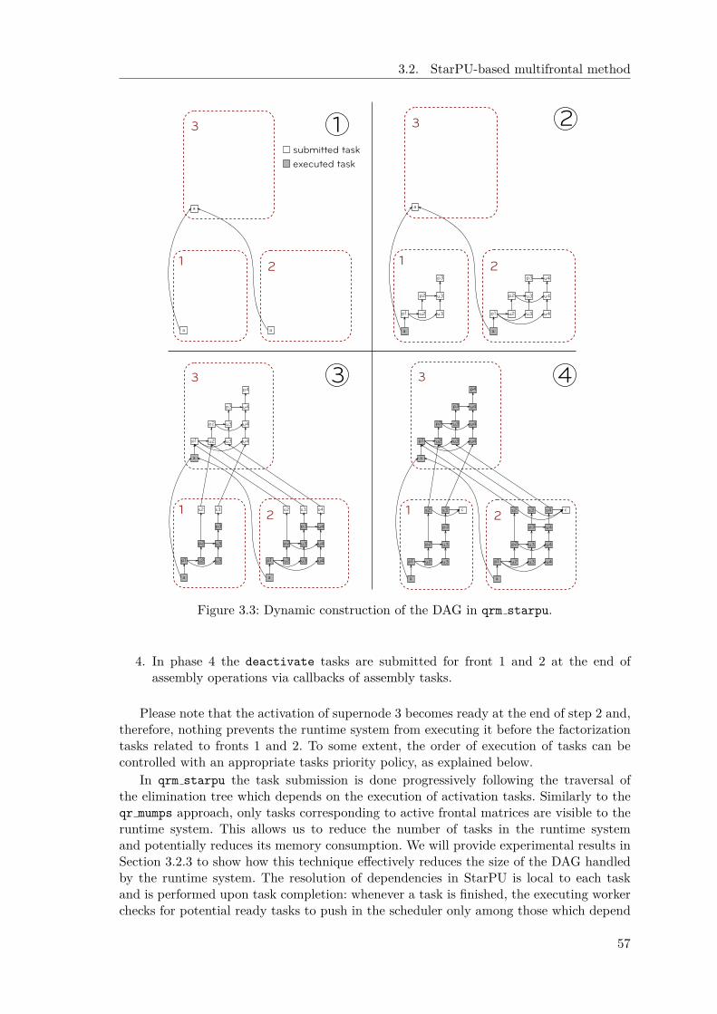
3.2. StarPU-based multifrontal method

Figure 3.3: Dynamic construction of the DAG in qrm starpu.

4. In phase 4 the deactivate tasks are submitted for front 1 and 2 at the end ofassembly operations via callbacks of assembly tasks.

Please note that the activation of supernode 3 becomes ready at the end of step 2 and,therefore, nothing prevents the runtime system from executing it before the factorizationtasks related to fronts 1 and 2. To some extent, the order of execution of tasks can becontrolled with an appropriate tasks priority policy, as explained below.

In qrm starpu the task submission is done progressively following the traversal ofthe elimination tree which depends on the execution of activation tasks. Similarly to theqr mumps approach, only tasks corresponding to active frontal matrices are visible to theruntime system. This allows us to reduce the number of tasks in the runtime systemand potentially reduces its memory consumption. We will provide experimental results inSection 3.2.3 to show how this technique effectively reduces the size of the DAG handledby the runtime system. The resolution of dependencies in StarPU is local to each taskand is performed upon task completion: whenever a task is finished, the executing workerchecks for potential ready tasks to push in the scheduler only among those which depend

57

3. Task-based multifrontal method: porting on a general purpose

runtime system

on it. As a result, the tracking and updating of dependencies has a much smaller cost thanthe method implemented in qr mumps; most importantly, this cost only depends on thenumber of outgoing edges of each task and is, therefore, relatively independent of the sizeof the input sparse problem.

There is one fundamental difference between qr mumps and qrm starpu. In the mul-tifrontal QR method, the assembly of a front is an embarrassingly parallel operationbecause it simply consists in the copy of coefficients of the contribution blocks from thechild nodes into different locations in the front. This means that any two assembly taskscan be done in any order and possibly in parallel even though they access the same block-column. qr mumps can easily take advantage of this fact because the task dependenciesare hard-coded in the fill queues routine based on the knowledge of the algorithm. Inqrm starpu, instead, if two or more assembly tasks access the same block-column, a data-hazard is detected and thus the tasks are serialized according to the order of submission.In order to partially address this problem, the StarPU developers implemented a novel ac-cess mode STARPU COMMUTE which makes it possible to instruct the runtime system aboutthe possibility of executing two tasks in any order (but not in parallel).

This is an example of how our developments and evaluations provide valuable feedbackto the community of runtime systems developers; we will show other examples of this fruit-ful collaboration in the next sections. This feature, however, was not yet available at themoment we implemented qrm starpu and ran the experiments in Section 3.2.3; the com-mutativity among assembly tasks was instead used in the work described in Chapters 4, 5and 6.

3.2.2 Dynamic task scheduling and memory consumption

The level of concurrency as well as the memory consumption of the multifrontal methodbased on StarPU depend on the path followed in the DAG and the scheduling policyused. As explained, the numerical tasks (i.e., panel reductions, updates and assemblies)are submitted by activation tasks which are, therefore, extremely important because theypotentially increase the concurrency level and enhance the scalability. It must be noted,however, that executing an activation task too early is worthless because the numericaltasks it submits cannot be executed as they depend on many other, previously submittedtasks. On the other hand, the activation tasks in charge of allocating fronts increase thememory consumption. For this reason, during the dynamic construction of the DAG weneed an efficient scheduling policy to have an amount of concurrency suited to the resourcesand to save memory from unnecessary allocations.

Maximizing concurrency while limiting the memory consumption is achieved by as-signing to each type of tasks priority values as follows:

• activate: This tasks increases the memory consumption by allocating frontal matrixdata structures and therefore we assign it a negative priority to prevent the schedulerfrom allocating fronts when there is enough parallelism to feed all resources and thuslimit memory consumption;

• assemble: These tasks are critical for concurrency because all numerical tasks froma front depend on it. They are given the highest priority after deactivate operationwhich is 3;

• geqrt: panel operations lie on the critical path of the DAG corresponding to thedense QR factorization when using a 1D block-column partitioning. They are as-signed priority 2 which is higher than non-critical update tasks;

58

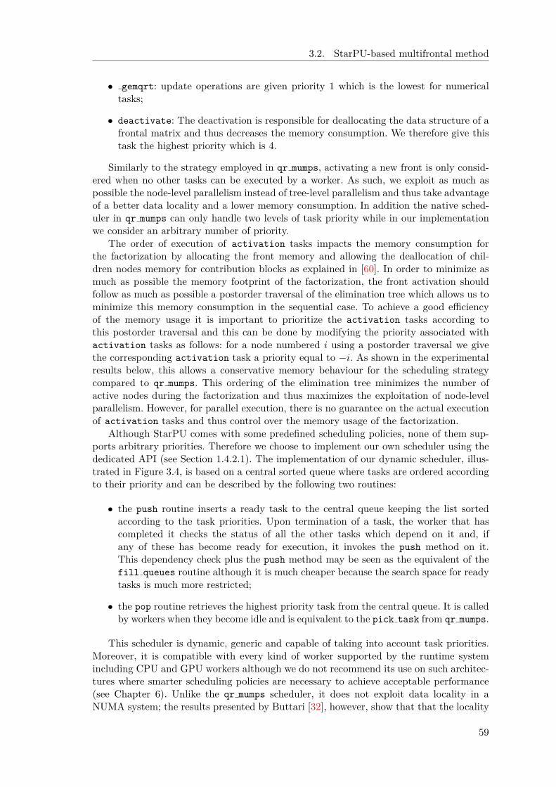
3.2. StarPU-based multifrontal method

• gemqrt: update operations are given priority 1 which is the lowest for numericaltasks;

• deactivate: The deactivation is responsible for deallocating the data structure of afrontal matrix and thus decreases the memory consumption. We therefore give thistask the highest priority which is 4.

Similarly to the strategy employed in qr mumps, activating a new front is only consid-ered when no other tasks can be executed by a worker. As such, we exploit as much aspossible the node-level parallelism instead of tree-level parallelism and thus take advantageof a better data locality and a lower memory consumption. In addition the native sched-uler in qr mumps can only handle two levels of task priority while in our implementationwe consider an arbitrary number of priority.

The order of execution of activation tasks impacts the memory consumption forthe factorization by allocating the front memory and allowing the deallocation of chil-dren nodes memory for contribution blocks as explained in [60]. In order to minimize asmuch as possible the memory footprint of the factorization, the front activation shouldfollow as much as possible a postorder traversal of the elimination tree which allows us tominimize this memory consumption in the sequential case. To achieve a good efficiencyof the memory usage it is important to prioritize the activation tasks according tothis postorder traversal and this can be done by modifying the priority associated withactivation tasks as follows: for a node numbered i using a postorder traversal we givethe corresponding activation task a priority equal to −i. As shown in the experimentalresults below, this allows a conservative memory behaviour for the scheduling strategycompared to qr mumps. This ordering of the elimination tree minimizes the number ofactive nodes during the factorization and thus maximizes the exploitation of node-levelparallelism. However, for parallel execution, there is no guarantee on the actual executionof activation tasks and thus control over the memory usage of the factorization.

Although StarPU comes with some predefined scheduling policies, none of them sup-ports arbitrary priorities. Therefore we choose to implement our own scheduler using thededicated API (see Section 1.4.2.1). The implementation of our dynamic scheduler, illus-trated in Figure 3.4, is based on a central sorted queue where tasks are ordered accordingto their priority and can be described by the following two routines:

• the push routine inserts a ready task to the central queue keeping the list sortedaccording to the task priorities. Upon termination of a task, the worker that hascompleted it checks the status of all the other tasks which depend on it and, ifany of these has become ready for execution, it invokes the push method on it.This dependency check plus the push method may be seen as the equivalent of thefill queues routine although it is much cheaper because the search space for readytasks is much more restricted;

• the pop routine retrieves the highest priority task from the central queue. It is calledby workers when they become idle and is equivalent to the pick task from qr mumps.

This scheduler is dynamic, generic and capable of taking into account task priorities.Moreover, it is compatible with every kind of worker supported by the runtime systemincluding CPU and GPU workers although we do not recommend its use on such architec-tures where smarter scheduling policies are necessary to achieve acceptable performance(see Chapter 6). Unlike the qr mumps scheduler, it does not exploit data locality in aNUMA system; the results presented by Buttari [32], however, show that that the locality

59

3. Task-based multifrontal method: porting on a general purpose

runtime system

WorkersRuntime core

CPU0

CPU2

CPU1

task priority

t tt ...t

Scheduler

t

t

t

t

Figure 3.4: Sorted central queue scheduler in qrm starpu.

aware scheduling proposed therein (see Section 1.7.4.1) only provided mild improvementsand that an interleaved memory allocation policy does a much better job of reducing thepenalty for distant memory accesses on a limited size NUMA machine. A much bettermethod for dealing with the complexity of large NUMA machines is based on the conceptof contexts which was developed and evaluated by Hugo et al. [71, 70] and which we brieflydescribe in Section 7.3. Another drawback of this scheduler lies in the fact that all theready tasks are stored in a single queue: in the case were the number of ready tasks andof working threads is high, this may lead to a costly contention on the locks that preventconcurrent accesses to this data structure. In Section 4.4 we will describe the design andimplementation of a novel scheduler that aims at overcoming these shortcomings but webelieve that this scheduler provides the necessary features to conduct a fair comparisonwith the original qr mumps code.

3.2.3 Experimental results

This section aims at evaluating the effectiveness of the proposed techniques as well as theperformance of the resulting code. For this purpose, the behaviour of the qrm starpu codewill be compared to the original qr mumps and also, briefly, to the SuiteSparseQR package(referred to as spqr) released by Tim Davis in 2009 [42]. The tests were done on a subsetof the matrices in Table 1.1 on the Dude machine described in Section 1.9.1. Table 3.1shows the factorization times (in seconds) using qrm starpu, qr mumps and spqr withdifferent numbers of cores whereas Figure 3.5 presents the speedup achieved by each ofthese three solvers on 12 and 24 cores.

Both qr mumps and qrm starpu clearly outperform the spqr package by a factorgreater than two thanks to the powerful programming and execution paradigm basedon DAG parallelism. On the other hand, qrm starpu is consistently but only marginallyless efficient than qr mumps, by a factor below 10% for eight out of eleven matrices andstill only below 20% in the worst case. As a conclusion, the parallelization scheme im-pacts performance much more than the underlying low-level layer, validating the thesisthat modular approaches based on runtime systems can compete with heavily hand-tunedcodes.

For a better understanding of the behaviour of both qr mumps and qrm starpu, weconducted on both codes the analysis described in Section 2.1; the results of this analysisare reported on Figure 3.6. Please note that, for the purpose of this evaluation, the graphon the top-right corner of the figure reports the product of the granularity and the taskefficiencies eg × et as defined in Section 2.1 because these two metrics are expected to beequivalent for both codes as the results also prove. The granularity efficiency eg , in fact,is the same since the same values for the inner and outer blocking parameters (see Fig-ure 1.20) have been chosen for the two codes and thus exactly the same tasks are executedon both sides. As for the task efficiency et, it must be noted that all the experiments in

60

3.2. StarPU-based multifrontal method

Factorization time (sec.)

Matrix 1 2 3 4 5 6 7 8 9 10 11

th.

spqr

1 52.9 49.9 99.5 111.0 123.3 406.3 538.3 687.5 2081.0 4276.0 5361.02 34.5 32.1 63.4 69.0 74.1 238.1 290.1 379.1 1154.7 2870.4 2959.24 24.8 22.9 44.8 46.5 48.3 148.4 168.9 229.9 737.7 2001.0 1659.26 21.5 19.1 36.0 38.2 39.5 116.3 128.4 178.6 598.9 1845.9 1203.212 17.0 14.5 26.2 33.0 32.5 85.7 90.5 131.6 468.3 1644.0 769.918 15.7 12.7 22.5 28.8 29.1 73.4 78.7 119.1 404.9 1603.0 636.924 14.2 12.3 20.7 26.2 27.8 68.6 74.1 114.2 372.7 1389.3 588.6

qrm

starpu

1 51.8 49.0 97.5 104.8 137.5 417.6 496.1 733.6 1931.0 3572.0 5417.02 27.1 25.7 52.9 55.6 72.0 215.4 251.1 386.2 981.0 1813.0 2789.04 14.5 14.3 26.3 29.4 38.8 111.4 130.6 209.4 505.0 942.7 1410.06 10.6 10.2 18.9 20.8 27.2 77.9 91.6 153.7 349.9 676.0 979.412 6.9 6.2 10.9 12.4 16.2 43.4 50.4 92.4 190.3 439.3 525.818 6.0 5.0 9.0 9.8 13.1 32.0 38.1 69.1 146.3 363.7 371.124 5.7 4.4 8.0 8.5 12.4 28.1 32.9 58.0 122.7 336.3 305.9

qr

mumps

1 51.5 48.8 96.9 104.6 137.1 410.8 495.2 729.7 1928.0 3571.0 5420.02 26.1 24.5 51.1 53.6 69.1 208.4 248.7 368.8 969.4 1793.0 2724.04 13.7 12.7 25.0 27.0 35.6 105.1 125.6 189.8 505.0 903.9 1367.06 9.6 8.7 17.1 18.4 24.5 71.9 85.8 127.9 333.0 617.6 919.112 5.7 5.2 10.2 10.8 14.2 39.5 46.6 69.4 177.9 392.3 479.018 4.9 4.3 8.3 8.6 11.7 29.6 34.0 53.3 137.2 342.3 339.024 5.0 4.3 7.9 8.0 11.0 26.5 30.5 48.8 120.9 337.0 282.0

Table 3.1: Factorization times, in seconds, on an AMD Istanbul system for qrm starpu

(top), qr mumps (middle) and spqr (bottom). The first row shows the matrix number.

0

5

10

15

20

1 2 3 4 5 6 7 8 9 10 11

Matrix #

Speedup -- spqr vs qr_starpu vs qr_mumps

spqr 12 threads

qrs 12 threads

qrm 12 threads

spqr 24 threads

qrs 24 threads

qrm 24 threads

Figure 3.5: Speedup for the spqr, qrm starpu and qr mumps factorizations on 12 and 24cores.

61

3. Task-based multifrontal method: porting on a general purpose

runtime system

0

0.2

0.4

0.6

0.8

1

1 2 3 4 5 6 7 8 9 10 11

Overall efficiency

e qrm

e qrs

0

0.2

0.4

0.6

0.8

1

1 2 3 4 5 6 7 8 9 10 11

Granularity x Task efficiency

et qrm

et qrs

0

0.2

0.4

0.6

0.8

1

1 2 3 4 5 6 7 8 9 10 11

Pipeline efficiency

ep qrm

ep qrs

0

0.2

0.4

0.6

0.8

1

1 2 3 4 5 6 7 8 9 10 11

Runtime efficiency

er qrm

er qrs

Figure 3.6: Efficiency measures for qr mumps (qrm) and qrm starpu (qrs).

62

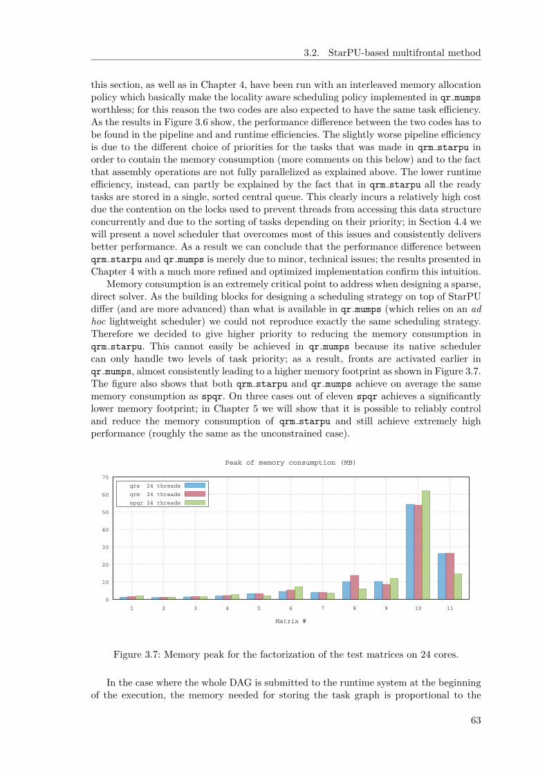
3.2. StarPU-based multifrontal method

this section, as well as in Chapter 4, have been run with an interleaved memory allocationpolicy which basically make the locality aware scheduling policy implemented in qr mumps

worthless; for this reason the two codes are also expected to have the same task efficiency.As the results in Figure 3.6 show, the performance difference between the two codes has tobe found in the pipeline and and runtime efficiencies. The slightly worse pipeline efficiencyis due to the different choice of priorities for the tasks that was made in qrm starpu inorder to contain the memory consumption (more comments on this below) and to the factthat assembly operations are not fully parallelized as explained above. The lower runtimeefficiency, instead, can partly be explained by the fact that in qrm starpu all the readytasks are stored in a single, sorted central queue. This clearly incurs a relatively high costdue the contention on the locks used to prevent threads from accessing this data structureconcurrently and due to the sorting of tasks depending on their priority; in Section 4.4 wewill present a novel scheduler that overcomes most of this issues and consistently deliversbetter performance. As a result we can conclude that the performance difference betweenqrm starpu and qr mumps is merely due to minor, technical issues; the results presented inChapter 4 with a much more refined and optimized implementation confirm this intuition.

Memory consumption is an extremely critical point to address when designing a sparse,direct solver. As the building blocks for designing a scheduling strategy on top of StarPUdiffer (and are more advanced) than what is available in qr mumps (which relies on an adhoc lightweight scheduler) we could not reproduce exactly the same scheduling strategy.Therefore we decided to give higher priority to reducing the memory consumption inqrm starpu. This cannot easily be achieved in qr mumps because its native schedulercan only handle two levels of task priority; as a result, fronts are activated earlier inqr mumps, almost consistently leading to a higher memory footprint as shown in Figure 3.7.The figure also shows that both qrm starpu and qr mumps achieve on average the samememory consumption as spqr. On three cases out of eleven spqr achieves a significantlylower memory footprint; in Chapter 5 we will show that it is possible to reliably controland reduce the memory consumption of qrm starpu and still achieve extremely highperformance (roughly the same as the unconstrained case).

0

10

20

30

40

50

60

70

1 2 3 4 5 6 7 8 9 10 11

Matrix #

Peak of memory consumption (MB)

qrs 24 threads

qrm 24 threads

spqr 24 threads

Figure 3.7: Memory peak for the factorization of the test matrices on 24 cores.

In the case where the whole DAG is submitted to the runtime system at the beginningof the execution, the memory needed for storing the task graph is proportional to the

63

3. Task-based multifrontal method: porting on a general purpose

runtime system

problem size. Figure 3.8 shows the maximum number of tasks that the runtime systemhandles during the factorization versus the total number of tasks executed. The firstbeing between 3 and 11 times smaller than the second, these data show that the techniqueproposed in Section 3.2 is effective in reducing the runtime system overhead and memoryconsumption.

0

20

40

60

80

100

120

140

160

180

200

1 2 3 4 5 6 7 8 9 10 11

Matrix #

Number of tasks (x1000)

max # of tasks

tot # of tasks

Figure 3.8: Maximum DAG size handled by StarPU during the factorization of the testmatrices when using 24 threads.

64

Chapter 4

STF-parallel multifrontal QRmethod on multicore architecture

In the previous chapter we proposed a first approach for the implementation of the mul-tifrontal QR method based on the StarPU runtime system which was mainly meant toasses the usability of a runtime system for implementing a sparse, direct method. Forthis reason we tried to reproduce as accurately as possible the behaviour of the originalqr mumps code. However, as explained at the end of Chapter 3, this implementation has anumber of shortcomings, most importantly the complexity and difficult maintainability ofthe code. For this reason, in this chapter, we develop and evaluate experimentally a novelapproach [S1] which implements the same algorithm (described in Section 1.7) in compli-ance with the Sequential Task Flow (STF) programming model presented in Section 1.4.1.We particularly emphasize the simplicity of the model for the parallelization of a complexalgorithm such as the multifrontal factorization method and show the effectiveness of theapproach.

We first illustrate the concept of the STF-parallelization of a sequential code withthe implementation of a multifrontal method without dealing with the choice of a frontpartitioning scheme. Then, we propose a STF-parallel multifrontal method using a 1Dblock-column partitioning and show both the effectiveness of the approach and the lim-itations arising from the choice of partitioning. Finally, by leveraging the expressivenessof the programming model, we enhance the exploitation of the node-level parallelism byintroducing dense 2D Communication Avoiding (CA) factorization algorithms of frontalmatrices. We show a substantial performance gain using this strategy with a small impacton the runtime overhead. It should be noted that the use of such factorization schemesin the multifrontal method represents a big challenge as it makes the DAG much biggerwith a more complex task dependency pattern. As previously discussed, we show that notonly the model facilitates the implementation of such features but also incurs a negligibleoverhead in the runtime system.

4.1 STF-parallel multifrontal QR method

4.1.1 STF-parallelization

In this section we present the STF parallelization of the multifrontal method without usingany specific frontal matrix partitioning. Figure 4.1 shows the main sequential pseudocodeof the factorization using the four basic kernels namely activate, assemble, deactivate

and factorize. This algorithms consists of a topological traversal of the elimination tree

65

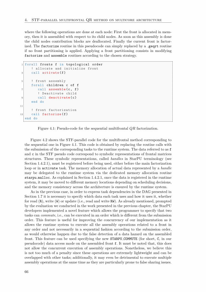
4. STF-parallel multifrontal QR method on multicore architecture

where the following operations are done at each node: First the front is allocated in mem-ory, then it is assembled with respect to its child nodes. As soon as this assembly is donethe child nodes contribution blocks are deallocated. Finally the current front is factor-ized. The factorize routine in this pseudocode can simply replaced by a geqrt routineif no front partitioning is applied. Applying a front partitioning consists in modifyingfactorize and assemble routines according to the chosen strategy.

1 forall fronts f in topological order

! allocate and initialize front

3 call activate (f)

5 ! front assembly

forall children c of f

7 call assemble (c, f)

! Deactivate child

9 call deactivate (c)

end do

11

! front factorization

13 call factorize (f)

end do

Figure 4.1: Pseudo-code for the sequential multifrontal QR factorization.

Figure 4.2 shows the STF-parallel code for the multifrontal method corresponding tothe sequential one in Figure 4.1. This code is obtained by replacing the routine calls withthe submission of the corresponding tasks to the runtime system. The data referred to as f

and c in the STF pseudo code correspond to symbolic representations of frontal matricesstructures. These symbolic representations, called handles in StarPU terminology (seeSection 1.4.2.1), must be registered before being used, either before the main factorizationloop or in activate task. The memory allocation of actual data represented by a handlemay be delegated to the runtime system via the dedicated memory allocation routinestarpu malloc. As explained in Section 1.4.2.1, once the data is registered in the runtimesystem, it may be moved to different memory locations depending on scheduling decisions,and the memory consistency across the architecture is ensured by the runtime system.

As in the previous case, in order to express task dependencies in the DAG presented inSection 1.7 it is necessary to specify which data each task uses and how it uses it, whetherfor read (R), write (W) or update (i.e., read and write RW). As already mentioned, promptedby the evaluation we conducted in the work presented in the previous chapter, the StarPUdevelopers implemented a novel feature which allows the programmer to specify that twotasks can commute, i.e., can be executed in an order which is different from the submissionorder. This feature is useful for improving the concurrency of our implementation as itallows the runtime system to execute all the assembly operations related to a front inany order and not necessarily in a sequential fashion according to the submission order,as would otherwise happen due to the false detection of a data hazard on the assembledfront. This feature can be used specifying the new STARPU COMMUTE (for short, C, in ourpseudocode) data access mode on the assembled front f. It must be noted that, this doesnot allow the concurrent execution of assembly operations. Nonetheless, we believe thisis not too much of a penalty since these operations are extremely lightweight and can beoverlapped with other tasks; additionally, it may even be detrimental to execute multipleassembly operations at the same time as they are particularly prone to false sharing issues.

66

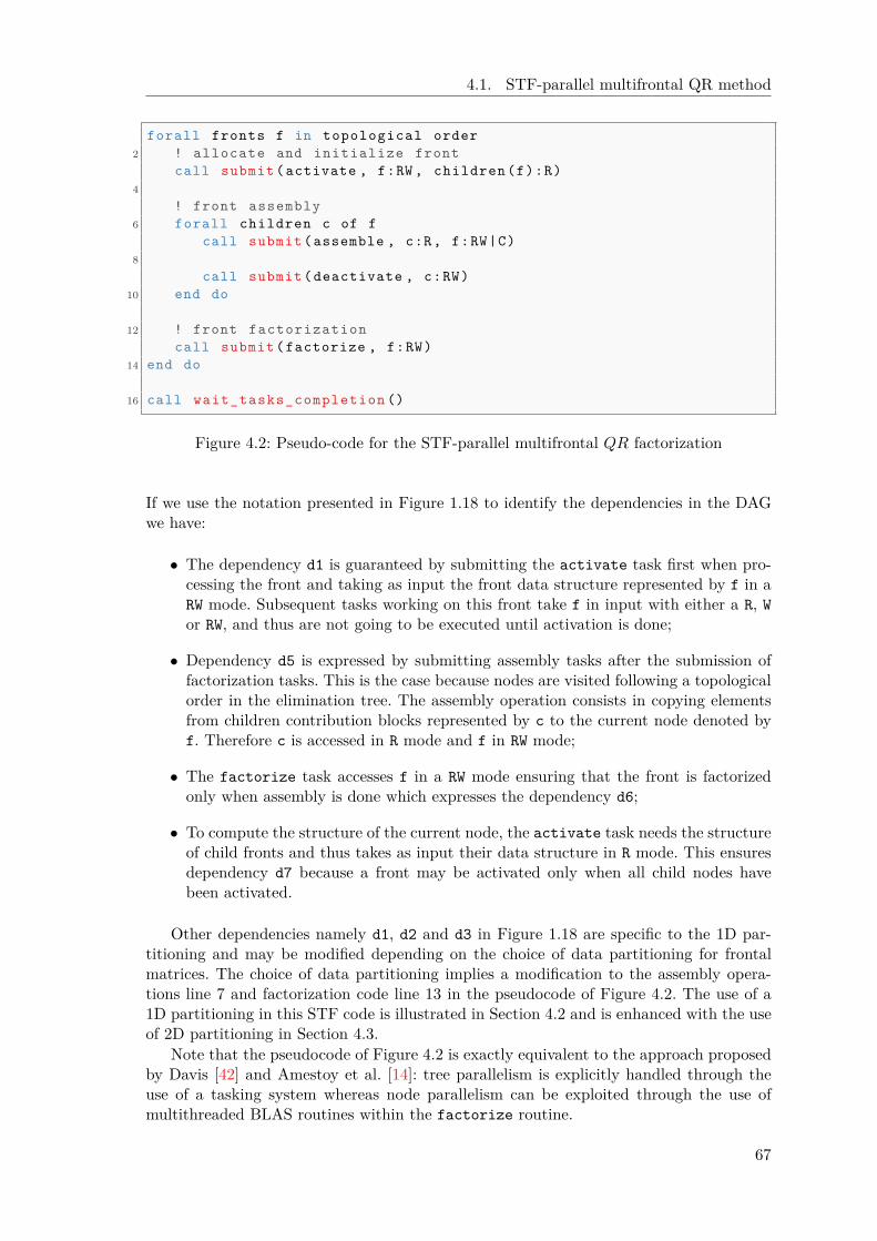
4.1. STF-parallel multifrontal QR method

forall fronts f in topological order

2 ! allocate and initialize front

call submit (activate , f:RW , children (f):R)

4

! front assembly

6 forall children c of f

call submit (assemble , c:R, f:RW|C)

8

call submit (deactivate , c:RW)

10 end do

12 ! front factorization

call submit (factorize , f:RW)

14 end do

16 call wait_tasks_completion ()

Figure 4.2: Pseudo-code for the STF-parallel multifrontal QR factorization

If we use the notation presented in Figure 1.18 to identify the dependencies in the DAGwe have:

• The dependency d1 is guaranteed by submitting the activate task first when pro-cessing the front and taking as input the front data structure represented by f in aRW mode. Subsequent tasks working on this front take f in input with either a R, W

or RW, and thus are not going to be executed until activation is done;

• Dependency d5 is expressed by submitting assembly tasks after the submission offactorization tasks. This is the case because nodes are visited following a topologicalorder in the elimination tree. The assembly operation consists in copying elementsfrom children contribution blocks represented by c to the current node denoted byf. Therefore c is accessed in R mode and f in RW mode;

• The factorize task accesses f in a RW mode ensuring that the front is factorizedonly when assembly is done which expresses the dependency d6;

• To compute the structure of the current node, the activate task needs the structureof child fronts and thus takes as input their data structure in R mode. This ensuresdependency d7 because a front may be activated only when all child nodes havebeen activated.

Other dependencies namely d1, d2 and d3 in Figure 1.18 are specific to the 1D par-titioning and may be modified depending on the choice of data partitioning for frontalmatrices. The choice of data partitioning implies a modification to the assembly opera-tions line 7 and factorization code line 13 in the pseudocode of Figure 4.2. The use of a1D partitioning in this STF code is illustrated in Section 4.2 and is enhanced with the useof 2D partitioning in Section 4.3.

Note that the pseudocode of Figure 4.2 is exactly equivalent to the approach proposedby Davis [42] and Amestoy et al. [14]: tree parallelism is explicitly handled through theuse of a tasking system whereas node parallelism can be exploited through the use ofmultithreaded BLAS routines within the factorize routine.

67

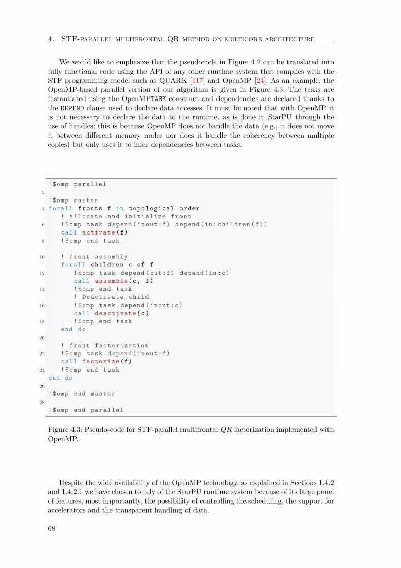
4. STF-parallel multifrontal QR method on multicore architecture

We would like to emphasize that the pseudocode in Figure 4.2 can be translated intofully functional code using the API of any other runtime system that complies with theSTF programming model such as QUARK [117] and OpenMP [24]. As an example, theOpenMP-based parallel version of our algorithm is given in Figure 4.3. The tasks areinstantiated using the OpenMPTASK construct and dependencies are declared thanks tothe DEPEND clause used to declare data accesses. It must be noted that with OpenMP itis not necessary to declare the data to the runtime, as is done in StarPU through theuse of handles; this is because OpenMP does not handle the data (e.g., it does not moveit between different memory nodes nor does it handle the coherency between multiplecopies) but only uses it to infer dependencies between tasks.

!$omp parallel

2

!$omp master

4 forall fronts f in topological order

! allocate and initialize front

6 !$omp task depend (inout:f) depend (in: children (f))

call activate (f)

8 !$omp end task

10 ! front assembly

forall children c of f

12 !$omp task depend (out:f) depend (in:c)

call assemble (c, f)

14 !$omp end task

! Deactivate child

16 !$omp task depend (inout:c)

call deactivate (c)

18 !$omp end task

end do

20

! front factorization

22 !$omp task depend (inout:f)

call factorize (f)

24 !$omp end task

end do

26

!$omp end master

28

!$omp end parallel

Figure 4.3: Pseudo-code for STF-parallel multifrontal QR factorization implemented withOpenMP.

Despite the wide availability of the OpenMP technology, as explained in Sections 1.4.2and 1.4.2.1 we have chosen to rely of the StarPU runtime system because of its large panelof features, most importantly, the possibility of controlling the scheduling, the support foraccelerators and the transparent handling of data.

68

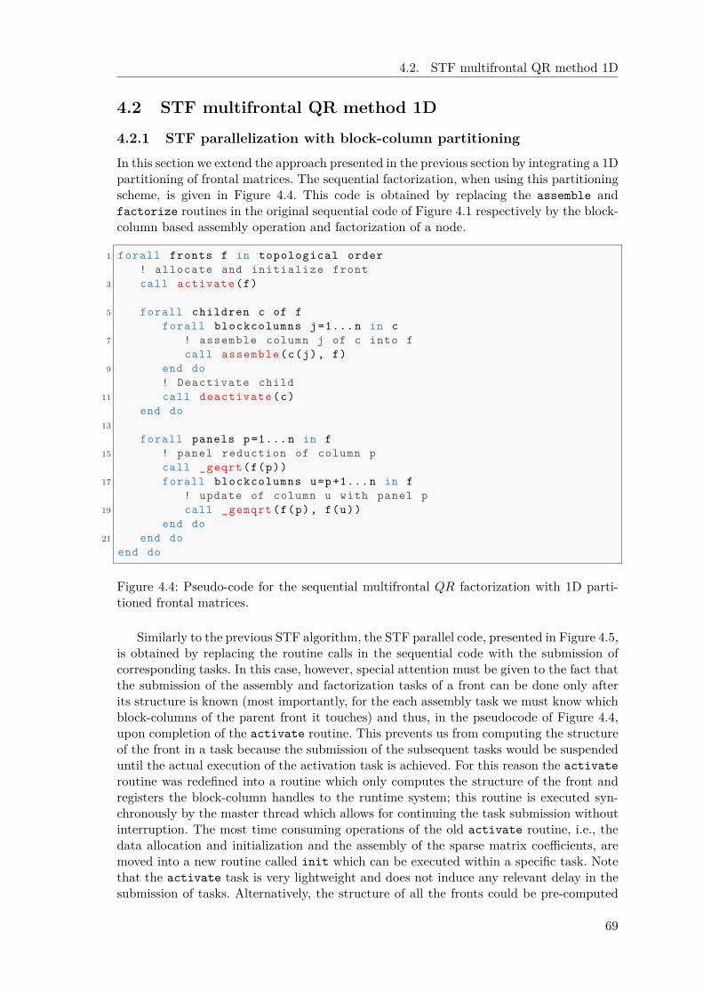
4.2. STF multifrontal QR method 1D

4.2 STF multifrontal QR method 1D

4.2.1 STF parallelization with block-column partitioning

In this section we extend the approach presented in the previous section by integrating a 1Dpartitioning of frontal matrices. The sequential factorization, when using this partitioningscheme, is given in Figure 4.4. This code is obtained by replacing the assemble andfactorize routines in the original sequential code of Figure 4.1 respectively by the block-column based assembly operation and factorization of a node.

1 forall fronts f in topological order

! allocate and initialize front

3 call activate (f)

5 forall children c of f

forall blockcolumns j=1...n in c

7 ! assemble column j of c into f

call assemble (c(j), f)

9 end do

! Deactivate child

11 call deactivate (c)

end do

13

forall panels p=1...n in f

15 ! panel reduction of column p

call _geqrt (f(p))

17 forall blockcolumns u=p+1...n in f

! update of column u with panel p

19 call _gemqrt (f(p), f(u))

end do

21 end do

end do

Figure 4.4: Pseudo-code for the sequential multifrontal QR factorization with 1D parti-tioned frontal matrices.

Similarly to the previous STF algorithm, the STF parallel code, presented in Figure 4.5,is obtained by replacing the routine calls in the sequential code with the submission ofcorresponding tasks. In this case, however, special attention must be given to the fact thatthe submission of the assembly and factorization tasks of a front can be done only afterits structure is known (most importantly, for the each assembly task we must know whichblock-columns of the parent front it touches) and thus, in the pseudocode of Figure 4.4,upon completion of the activate routine. This prevents us from computing the structureof the front in a task because the submission of the subsequent tasks would be suspendeduntil the actual execution of the activation task is achieved. For this reason the activate

routine was redefined into a routine which only computes the structure of the front andregisters the block-column handles to the runtime system; this routine is executed syn-chronously by the master thread which allows for continuing the task submission withoutinterruption. The most time consuming operations of the old activate routine, i.e., thedata allocation and initialization and the assembly of the sparse matrix coefficients, aremoved into a new routine called init which can be executed within a specific task. Notethat the activate task is very lightweight and does not induce any relevant delay in thesubmission of tasks. Alternatively, the structure of all the fronts could be pre-computed

69

4. STF-parallel multifrontal QR method on multicore architecture

during the analysis phase and stored but, as explained, this would result in excessivememory consumption.

forall fronts f in topological order

2 ! compute structure and register handles

call activate (f)

4

! allocate and initialize front

6 call submit (init , f:RW , children (f):R)

8 forall children c of f

forall blockcolumns j=1...n in c

10 ! assemble column j of c into f

call submit (assemble , c(j):R, f:RW|C)

12 end do

! Deactivate child

14 call submit (deactivate , c:RW)

end do

16

forall panels p=1...n in f

18 ! panel reduction of column p

call submit (_geqrt , f(p):RW)

20 forall blockcolumns u=p+1...n in f

! update of column u with panel p

22 call submit (_gemqrt , f(p):R, f(u):RW)

end do

24 end do

end do

26

call wait_tasks_completion ()

Figure 4.5: Pseudo-code for the STF-parallel multifrontal QR factorization with 1D par-titioned frontal matrices.

Using the data access modes and the order of task submission, the runtime systemautomatically infers dependencies between tasks and thus builds the DAG, specifically:

• the activation of a node f depends on the activation of its children;

• all the other tasks related to a node f depend on the node activation;

• the assembly of a block-column j of a front c into its parent f depends on all thegeqrt and gemqrt tasks on c(j) and on the activation of f;

• the geqrt task on a block-column p depends on all the assembly and all the previousupdate tasks concerning p;

• the gemqrt task on a block-column u with respect to geqrt p depends on all theassembly and all the previous gemqrt tasks concerning u and the related geqrt

task on block-column p;

• the deactivation of a front c can only be executed once all the related geqrt,gemqrt and assemble tasks are completed.

70

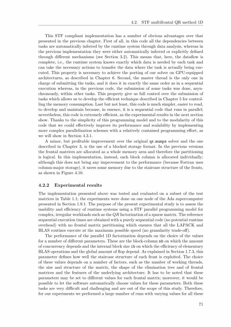
4.2. STF multifrontal QR method 1D

This STF compliant implementation has a number of obvious advantages over thatpresented in the previous chapter. First of all, in this code all the dependencies betweentasks are automatically inferred by the runtime system through data analysis, whereas inthe previous implementation they were either automatically inferred or explicitly definedthrough different mechanisms (see Section 3.2). This means that, here, the dataflow iscomplete, i.e., the runtime system knows exactly which data is needed by each task andcan take the necessary actions to transfer the data where the task is actually being exe-cuted. This property is necessary to achieve the porting of our solver on GPU-equippedarchitectures, as described in Chapter 6. Second, the master thread is the only one incharge of submitting the tasks, and it does it in exactly the same order as in a sequentialexecution whereas, in the previous code, the submission of some tasks was done, asyn-chronously, within other tasks. This property give us full control over the submission oftasks which allows us to develop the efficient technique described in Chapter 5 for control-ling the memory consumption. Last but not least, this code is much simpler, easier to read,to develop and maintain because, in essence, it is a sequential code that runs in parallel;nevertheless, this code is extremely efficient, as the experimental results in the next sectionshow. Thanks to the simplicity of this programming model and to the modularity of thiscode that we could effectively improve its performance and scalability by implementingmore complex parallelization schemes with a relatively contained programming effort, aswe will show in Section 4.3.1.

A minor, but profitable improvement over the original qr mumps solver and the onedescribed in Chapter 3, is the use of a blocked storage format. In the previous versionsthe frontal matrices are allocated as a whole memory area and therefore the partitioningis logical. In this implementation, instead, each block column is allocated individually;although this does not bring any improvement to the performance (because Fortran usescolumn-major storage), it saves some memory due to the staircase structure of the fronts,as shown in Figure 4.10.

4.2.2 Experimental results

The implementation presented above was tested and evaluated on a subset of the testmatrices in Table 1.1; the experiments were done on one node of the Ada supercomputerpresented in Section 1.9.1. The purpose of the present experimental study is to assess theusability and efficiency of runtime systems using a STF parallel programming model forcomplex, irregular workloads such as the QR factorization of a sparse matrix. The referencesequential execution times are obtained with a purely sequential code (no potential runtimeoverhead) with no frontal matrix partitioning which ensures that all the LAPACK andBLAS routines execute at the maximum possible speed (no granularity trade-off).

The performance of the parallel 1D factorization depends on the choice of the valuesfor a number of different parameters. These are the block-column nb on which the amountof concurrency depends and the internal block size ib on which the efficiency of elementaryBLAS operations and the global amount of flop depend. As explained in Section 1.7.3, thisparameter defines how well the staircase structure of each front is exploited. The choiceof these values depends on a number of factors, such as the number of working threads,the size and structure of the matrix, the shape of the elimination tree and of frontalmatrices and the features of the underlying architecture. It has to be noted that theseparameters may be set to different values for each frontal matrix; moreover, it would bepossible to let the software automatically choose values for these parameters. Both thesetasks are very difficult and challenging and are out of the scope of this study. Therefore,for our experiments we performed a large number of runs with varying values for all these

71

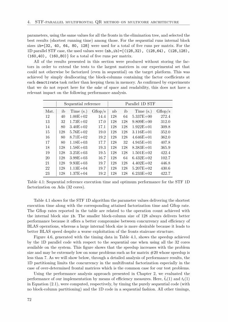
4. STF-parallel multifrontal QR method on multicore architecture

parameters, using the same values for all the fronts in the elimination tree, and selected thebest results (shortest running time) among those. For the sequential runs internal blocksizes ib={32, 40, 64, 80, 128} were used for a total of five runs per matrix. For the1D parallel STF case, the used values were (nb,ib)={(128,32), (128,64), (128,128),

(160,40), (160,80)} for a total of five runs per matrix.

All of the results presented in this section were produced without storing the fac-tors in order to extend the tests to the largest matrices in our experimental set thatcould not otherwise be factorized (even in sequential) on the target platform. This wasachieved by simply deallocating the block-columns containing the factor coefficients ateach deactivate task rather than keeping them in memory. As confirmed by experimentsthat we do not report here for the sake of space and readability, this does not have arelevant impact on the following performance analysis.

Sequential reference Parallel 1D STF

Mat. ib Time (s.) Gflop/s nb ib Time (s.) Gflop/s12 40 1.00E+02 14.4 128 64 5.337E+00 272.413 32 1.73E+02 17.0 128 128 9.809E+00 312.014 80 3.40E+02 17.1 128 128 1.922E+01 309.815 128 5.76E+02 19.0 128 128 3.116E+01 352.016 80 8.71E+02 19.2 128 128 4.646E+01 362.017 80 1.18E+03 17.7 128 32 4.945E+01 407.818 128 1.58E+03 19.3 128 128 8.383E+01 365.919 128 3.25E+03 19.5 128 128 1.501E+02 422.420 128 3.99E+03 16.7 128 64 6.432E+02 102.721 128 9.93E+03 19.7 128 128 4.402E+02 446.822 128 1.13E+04 19.7 128 128 5.207E+02 430.623 128 1.37E+04 19.2 128 128 6.233E+02 422.7

Table 4.1: Sequential reference execution time and optimum performance for the STF 1Dfactorization on Ada (32 cores).

Table 4.1 shows for the STF 1D algorithm the parameter values delivering the shortestexecution time along with the corresponding attained factorization time and Gflop rate.The Gflop rates reported in the table are related to the operation count achieved withthe internal block size ib. The smaller block-column size of 128 always delivers betterperformance because it offers a better compromise between concurrency and efficiency ofBLAS operations, whereas a large internal block size is more desirable because it leads tobetter BLAS speed despite a worse exploitation of the fronts staircase structure.

Figure 4.6, generated with the timing data in Table 4.1, shows the speedup achievedby the 1D parallel code with respect to the sequential one when using all the 32 coresavailable on the system. This figure shows that the speedup increases with the problemsize and may be extremely low on some problems such as for matrix #20 whose speedup isless than 7. As we will show below, through a detailed analysis of performance results, the1D partitioning limits the concurrency in the multifrontal factorization especially in thecase of over-determined frontal matrices which is the common case for our test problems.

Using the performance analysis approach presented in Chapter 2, we evaluated theperformance of our implementation by means of efficiency measures. Here, tt(1) and tt(1)in Equation (2.1), were computed, respectively, by timing the purely sequential code (withno block-column partitioning) and the 1D code in a sequential fashion. All other timings,

72

4.2. STF multifrontal QR method 1D

0

5

10

15

20

25

30

12 13 14 15 16 17 18 19 20 21 22 23

Matrix #

Speedup 1D -- 32 cores

1D

Figure 4.6: Speedup of the STF 1D algorithm with respect to the sequential case on Ada(32 cores).

i.e. tr(p), tc(p) and ti(p) are returned by StarPU upon execution of the parallel code with1D block-column partitioning on p = 32 cores. All these measurements are related to theparameter settings in Table 4.1.

The 1D partitioning provides a coarse granularity of tasks resulting in a good granular-ity efficiency with a value greater than 0.8 on the tested problems. However it suffers frompoor cache behaviour in the case of extremely overdetermined frontal matrices becauseof the tall-and-skinny shape of block-columns. This phenomenon is accentuated when theproblem grows which explains the decrease of the granularity efficiency when the matrixsize increases. As shown in Figure 4.7, the lowest granularity efficiency is obtained on thematrix #20 which represents an extreme case for the impact of overdetermined matricesbecause most of the flops are done in one front with roughly 1.3 M rows and only 7 Kcolumns. The performance loss induced by the runtime is extremely small in our case withan overhead lower than 2% on average showing the efficiency of our scheduling strategy.

The efficiency results in Figure 4.7 show that the most limiting factors for the scal-ability of the factorization are the impact of data locality and the task pipelining. Asexplained for the efficiency of granularity, data locality may not be efficiently exploitedbecause of the 1D partitioning which does not allows for a good exploitation of low-levelmemory resulting in performance loss during parallel execution due to memory contentionand inter-level communications. The relatively poor pipeline efficiency obtained on smallermatrices is due to the limited amount of concurrency offered by the 1D partitioning espe-cially for overdetermined matrices. This lack of parallelism is compensated by the tree-levelparallelism and is thus less evident on large problems. As expected the matrix #20 givesextremely low pipeline efficiency resulting from the low concurrency level provided by the1D partitioning on a tall-and-skinny matrix.

73

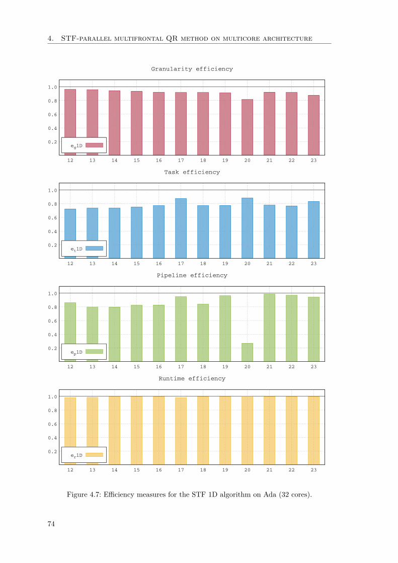
4. STF-parallel multifrontal QR method on multicore architecture

0.2

0.4

0.6

0.8

1.0

12 13 14 15 16 17 18 19 20 21 22 23

Granularity efficiency

eg1D

0.2

0.4

0.6

0.8

1.0

12 13 14 15 16 17 18 19 20 21 22 23

Task efficiency

et1D

0.2

0.4

0.6

0.8

1.0

12 13 14 15 16 17 18 19 20 21 22 23

Pipeline efficiency

ep1D

0.2

0.4

0.6

0.8

1.0

12 13 14 15 16 17 18 19 20 21 22 23

Runtime efficiency

er1D

Figure 4.7: Efficiency measures for the STF 1D algorithm on Ada (32 cores).

74

4.2. STF multifrontal QR method 1D

4.2.3 The effect of inter-level parallelism

As explained in Section 1.7, qr mumps and qrm starpu can take advantage of what wecalled inter-level parallelism which allows for working on a block-column of a front assoon as it becomes fully assembled regardless of the status of the other block-columnswithin the same front or within child fronts. As a result, the factorization of a front can bepipelined with those of the child nodes for an extra source of parallelism. This techniqueis rather complex to implement as it requires tracking the assembly status of each columnindividually; in qrm starpu this is implicitly and very efficiently done by the runtimesystem through the tracking of dependencies between tasks.

Although the elimination tree can be traversed in any topological order, a postorderis commonly chosen because it has favorable properties in terms of memory consumption.In a parallel execution the traversal deviates from this postorder in order to use treeparallelism and achieve better concurrency but, if possible, it is better to stay as closeas possible to the sequential postorder in order to avoid excessive memory consumption.This can be achieved in a relatively easy way in a share memory context using techniqueslike the one presented in Section 3.2.2 but it is much more complex in a distributedmemory parallel setting (see, for example, the work by Agullo et al. [2]). As a result,in a shared memory parallel multifrontal solver, the factorization can be imagined asa wavefront which starts from one corner of the elimination tree, say, the bottom leftcorner, and sweeps the entire tree moving towards the opposite corner, the top right one.When this wavefront reaches the last, rightmost branch, all the fronts therein are treatedsequentially, one after the other because no tree parallelism is available anymore. Thislack of concurrency can incur a severe penalty if the inter-level parallelism is not usedbecause quite a considerable fraction of the total volume of operations is done on theselast fronts. Figure 4.8 shows, on the top part, the execution trace for the factorizationof matrix #5 on the Dude machine when inter-level parallelism is not implemented. Thistrace was produced by adding “fake” dependencies to the qrm starpu solver in order toreproduce the behaviour shown in Figure 1.16 (right). A different color has been used forall the tasks related to each front. It is seen visible how the lack of tree parallelism on thelast few fronts introduces a heavy penalty stall in the execution traces. On the contrary,when inter-level parallelism is implemented, the execution trace (see the bottom trace inFigure 4.8) is relatively densely populated until the end of the execution leading to a gainin time of around 30%.

Because the runtime controls all the components of the parallel execution of a code,from the execution of tasks to the handling of their mutual dependencies, it can provideaccurate measurement and data that allow for detailed performance analysis. Specifically,the StarPU runtime system can produce the DAG that includes all the tasks along withtheir dependencies where the tasks can be weighted with either their execution time orother useful information provided by the programmer. Using these data, we conducted acritical-path analysis for the factorization of our test matrices using the STF parallel code.Assuming that the critical path (the longest path in the DAG) is a lower bound on theexecution time, the maximum achievable speedup or average degree of concurrency canbe defined as the ratio between the sum of the weights of all the tasks along the criticalpath (i.e., length of the critical path) and the sum of the weights in the whole DAG:

max speedup = avg concurrency =

∑i∈DAG wi∑i∈CP wi

where wi is the weight of task i. For each matrix, the DAG used to conduct thisanalysis is the one related to the case where 32 working threads are used (remember that

75

4. STF-parallel multifrontal QR method on multicore architecture

Time

Figure 4.8: Execution traces for matrix #5 on the Dude architectures using 24 coreswithout (top) and with (bottom) inter-level parallelism.

the DAG changes with the number of threads because of a different choice of the tree-pruning level as described in Section 1.7.2). The weight of tasks is chosen to be equal tothe execution time measured in an execution with only one working thread. This precisechoice was made because we believe that granularity plays an important role in the criticalpath analysis and thus the execution time is a more realistic measure than, for example,the number of flops (or the amount of data movement for memory-bound tasks); at thesame time, the single-threaded execution was chosen to exclude from the analysis theeffects of data locality (the reader can refer to Figure 4.7 for a measure of those). Thecritical path in the DAG is computed through a Depth-First Search. Figure 4.9 shows themaximum achievable speedup for the factorization of the test matrices using the methodpresented above, with or without inter-level parallelism. The figure shows that the inter-level parallelism is beneficial (considerably, for some problems such as #19 or #22) in allcases except for matrices #17 and #20. On these two problems the inter-level parallelismdoes not bring any benefit for different reasons. In matrix #17 all the largest fronts, exceptthe root, are largely underdetermined which means that concurrency is abundant withineach front and thus the lack of pipelining between fronts along the last branch is notpenalizing. In matrix #20, instead, most of the flops are performed in a single, huge frontand thus the benefit of inter-level parallelism is only marginal.

4.3 STF multifrontal QR method 2D

With a 1D partitioning of frontal matrices, the node parallelism is achieved because all theupdates related to a panel can be executed concurrently and because panel operations canbe executed at the same time as updates related to previous panels (this technique is well

76

4.3. STF multifrontal QR method 2D

0

20

40

60

80

100

120

140

160

12 13 14 15 16 17 18 19 20 21 22 23

Matrix #

Max degree of concurrency 1D

1D nopipe

1D pipe

Figure 4.9: Maximum degree of concurrency on Ada (32 cores) emerging from the DAGwith and without inter-level parallelism.

known under the name of lookahead). It is clear that when frontal matrices are stronglyoverdetermined (i.e., they have many more rows than columns, which is the most commoncase in the multifrontal QR method) this approach does not provide much concurrency.In the multifrontal method this problem is mitigated by the fact that multiple frontalmatrices are factorized at the same time. However, considering that in the multifrontalfactorization most of the computational weight is related to the topmost nodes wheretree parallelism is scarce, a 1D front factorization approach can still seriously limit thescalability as shown in the previous section.

1D Partitioning 2D Partitioning

nb

mb

nb

Figure 4.10: 1D partitioning of a frontal matrix into block-columns (left), 2D partitioninginto tiles (right) with blocked storage.

This severe limitation can be overcome by employing communication-avoiding algo-rithms for the factorization of frontal matrices. These methods, discussed in Section 1.3.1,

77

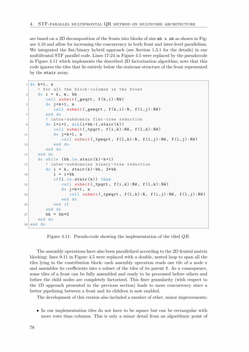
4. STF-parallel multifrontal QR method on multicore architecture

are based on a 2D decomposition of the fronts into blocks of size mb x nb as shown in Fig-ure 4.10 and allow for increasing the concurrency in both front and inter-level parallelism.We integrated the flat/binary hybrid approach (see Section 1.3.1 for the details) in ourmultifrontal STF parallel code. Lines 17-24 in Figure 4.5 were replaced by the pseudocodein Figure 4.11 which implements the described 2D factorization algorithm; note that thiscode ignores the tiles that lie entirely below the staircase structure of the front representedby the stair array.

1 do k=1, n

! for all the block - columns in the front

3 do i = k, m, bh

call submit (_geqrt , f(k,i):RW)

5 do j=k+1, n

call submit (_gemqrt , f(k,i):R, f(i,j):RW)

7 end do

! intra - subdomain flat -tree reduction

9 do l=i+1, min(i+bh -1, stair(k))

call submit (_tpqrt , f(i,k):RW , f(l,k):RW)

11 do j=k+1, n

call submit (_tpmqrt , f(l,k):R, f(i,j):RW , f(l,j):RW)

13 end do

end do

15 end do

do while (bh.le.stair(k)-k+1)

17 ! inter - subdomains binary -tree reduction

do i = k, stair(k)-bh , 2*bh

19 l = i+bh

if(l.le.stair(k)) then

21 call submit (_tpqrt , f(i,k):RW , f(l,k):RW)

do j=k+1, n

23 call submit (_tpmqrt , f(l,k):R, f(i,j):RW , f(l,j):RW)

end do

25 end if

end do

27 bh = bh*2

end do

29 end do

Figure 4.11: Pseudo-code showing the implementation of the tiled QR.

The assembly operations have also been parallelized according to the 2D frontal matrixblocking: lines 9-11 in Figure 4.5 were replaced with a double, nested loop to span all thetiles lying in the contribution block: each assembly operation reads one tile of a node c

and assembles its coefficients into a subset of the tiles of its parent f. As a consequence,some tiles of a front can be fully assembled and ready to be processed before others andbefore the child nodes are completely factorized. This finer granularity (with respect tothe 1D approach presented in the previous section) leads to more concurrency since abetter pipelining between a front and its children is now enabled.

The development of this version also included a number of other, minor improvements:

• In our implementation tiles do not have to be square but can be rectangular withmore rows than columns. This is only a minor detail from an algorithmic point of

78

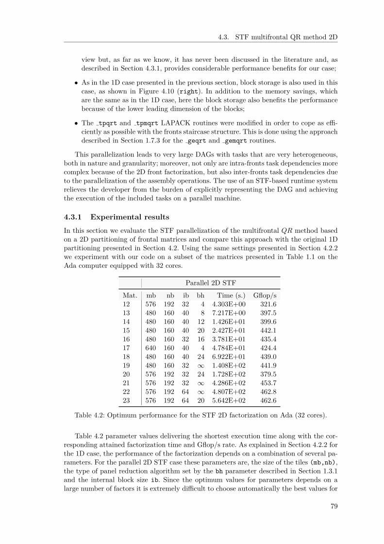
4.3. STF multifrontal QR method 2D

view but, as far as we know, it has never been discussed in the literature and, asdescribed in Section 4.3.1, provides considerable performance benefits for our case;

• As in the 1D case presented in the previous section, block storage is also used in thiscase, as shown in Figure 4.10 (right). In addition to the memory savings, whichare the same as in the 1D case, here the block storage also benefits the performancebecause of the lower leading dimension of the blocks;

• The tpqrt and tpmqrt LAPACK routines were modified in order to cope as effi-ciently as possible with the fronts staircase structure. This is done using the approachdescribed in Section 1.7.3 for the geqrt and gemqrt routines.

This parallelization leads to very large DAGs with tasks that are very heterogeneous,both in nature and granularity; moreover, not only are intra-fronts task dependencies morecomplex because of the 2D front factorization, but also inter-fronts task dependencies dueto the parallelization of the assembly operations. The use of an STF-based runtime systemrelieves the developer from the burden of explicitly representing the DAG and achievingthe execution of the included tasks on a parallel machine.

4.3.1 Experimental results

In this section we evaluate the STF parallelization of the multifrontal QR method basedon a 2D partitioning of frontal matrices and compare this approach with the original 1Dpartitioning presented in Section 4.2. Using the same settings presented in Section 4.2.2we experiment with our code on a subset of the matrices presented in Table 1.1 on theAda computer equipped with 32 cores.

Parallel 2D STF

Mat. mb nb ib bh Time (s.) Gflop/s12 576 192 32 4 4.303E+00 321.613 480 160 40 8 7.217E+00 397.514 480 160 40 12 1.426E+01 399.615 480 160 40 20 2.427E+01 442.116 480 160 32 16 3.781E+01 435.417 640 160 40 4 4.784E+01 424.418 480 160 40 24 6.922E+01 439.019 480 160 32 ∞ 1.408E+02 441.920 576 192 32 24 1.728E+02 379.521 576 192 32 ∞ 4.286E+02 453.722 576 192 64 ∞ 4.807E+02 462.823 576 192 64 20 5.642E+02 462.6

Table 4.2: Optimum performance for the STF 2D factorization on Ada (32 cores).

Table 4.2 parameter values delivering the shortest execution time along with the cor-responding attained factorization time and Gflop/s rate. As explained in Section 4.2.2 forthe 1D case, the performance of the factorization depends on a combination of several pa-rameters. For the parallel 2D STF case these parameters are, the size of the tiles (mb,nb),the type of panel reduction algorithm set by the bh parameter described in Section 1.3.1and the internal block size ib. Since the optimum values for parameters depends on alarge number of factors it is extremely difficult to choose automatically the best values for

79

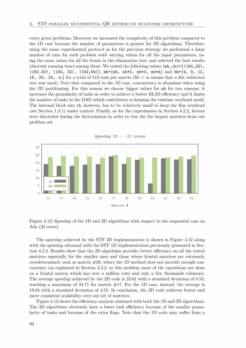
4. STF-parallel multifrontal QR method on multicore architecture

every given problems. Moreover we increased the complexity of this problem compared tothe 1D case because the number of parameters is greater for 2D algorithms. Therefore,using the same experimental protocol as for the previous strategy we performed a largenumber of runs for each problem with varying values for all the input parameters, us-ing the same values for all the fronts in the elimination tree, and selected the best results(shortest running time) among those. We tested the following values (nb,ib)={(160,32),

(160,40), (192, 32), (192,64)}, mb={nb, nb*2, nb*3, nb*4} and bh={4, 8, 12,

16, 20, 24, ∞} for a total of 112 runs per matrix (bh = ∞ means that a flat reductiontree was used). Note that compared to the 1D case, concurrency is abundant when usingthe 2D partitioning. For this reason we choose bigger values for nb for two reasons: itincreases the granularity of tasks in order to achieve a better BLAS efficiency and it limitsthe number of tasks in the DAG which contributes to keeping the runtime overhead small.The internal block size ib, however, has to be relatively small to keep the flop overhead(see Section 1.3.1) under control. Finally, as for the experiments in Section 4.2.2, factorswere discarded during the factorization in order to test the the largest matrices from ourproblem set.

0

5

10

15

20

25

30

12 13 14 15 16 17 18 19 20 21 22 23

Matrix #

Speedup 2D -- 32 cores

1D

2D

Figure 4.12: Speedup of the 1D and 2D algorithms with respect to the sequential case onAda (32 cores).

The speedup achieved by the STF 2D implementation is shown in Figure 4.12 alongwith the speedup obtained with the STF 1D implementation previously presented in Sec-tion 4.2.2. Results show that the 2D algorithm provides better efficiency on all the testedmatrices especially for the smaller ones and those where frontal matrices are extremelyoverdetermined, such as matrix #20, where the 1D method does not provide enough con-currency (as explained in Section 4.2.2, in this problem most of the operations are doneon a frontal matrix which has over a million rows and only a few thousands columns).The average speedup achieved by the 2D code is 23.61 with a standard deviation of 0.53,reaching a maximum of 24.71 for matrix #17. For the 1D case, instead, the average is19.04 with a standard deviation of 4.55. In conclusion, the 2D code achieves better andmore consistent scalability over our set of matrices.

Figure 4.13 shows the efficiency analysis obtained with both the 1D and 2D algorithms.The 2D algorithms obviously have a lower task efficiency because of the smaller granu-larity of tasks and because of the extra flops. Note that the 1D code may suffer from a

80

4.3. STF multifrontal QR method 2D

poor cache behaviour in the case of extremely overdetermined frontal matrices because ofthe extremely tall-and-skinny shape of block-columns. This explains why the granularityefficiency for the 2D code on matrix #20 is better than for the 1D code unlike for the othermatrices. 2D algorithms, however, achieve better locality efficiency than 1D most likelydue to the 2D partitioning of frontal matrices into tiles which have a more cache-friendlyshape and size than the extremely tall and skinny block-columns used in the 1D algo-rithm. Not surprisingly, the 2D code achieves much better scheduling efficiency (i.e., lessidle time) than the 1D code on all matrices: this results from a much higher concurrency,which is the purpose of the 2D code. As for the runtime efficiency, it is in favor of the1D implementation due to a much smaller number of tasks with bigger granularity andsimpler dependencies. However the performance loss induced by the runtime is extremelysmall in both cases: less than 2% on average and never higher than 4% for the 2D imple-mentation; this is also due to the efficiency of the scheduler specifically implemented andused for these experiments (see Section 4.4).

81

4. STF-parallel multifrontal QR method on multicore architecture

0.2

0.4

0.6

0.8

1.0

12 13 14 15 16 17 18 19 20 21 22 23

Granularity efficiency

eg1D

eg2D

0.2

0.4

0.6

0.8

1.0

12 13 14 15 16 17 18 19 20 21 22 23

Task efficiency

et1D

et2D

0.2

0.4

0.6

0.8

1.0

12 13 14 15 16 17 18 19 20 21 22 23

Pipeline efficiency

ep1D

ep2D

0.2

0.4

0.6

0.8

1.0

12 13 14 15 16 17 18 19 20 21 22 23

Runtime efficiency

er1D

er2D

Figure 4.13: Efficiency measures for the STF 1D algorithm on Ada (32 cores).

82

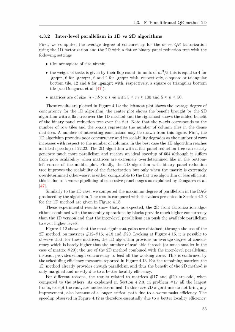
4.3. STF multifrontal QR method 2D

4.3.2 Inter-level parallelism in 1D vs 2D algorithms

First, we computed the average degree of concurrency for the dense QR factorizationusing the 1D factorization and the 2D with a flat or binary panel reduction tree with thefollowing settings

• tiles are square of size nbxnb;

• the weight of tasks is given by their flop count: in units of nb3/3 this is equal to 4 forgeqrt, 6 for gemqrt, 6 and 2 for geqrt with, respectively, a square or triangularbottom tile, 12 and 6 for gemqrt with, respectively, a square or triangular bottomtile (see Dongarra et al. [47]);

• matrices are of size m ∗ nb × n ∗ nb with 5 ≤ m ≤ 100 and 5 ≤ n ≤ 50.

These results are plotted in Figure 4.14: the leftmost plot shows the average degree ofconcurrency for the 1D algorithm, the center plot shows the benefit brought by the 2Dalgorithm with a flat tree over the 1D method and the rightmost shows the added benefitof the binary panel reduction tree over the flat. Note that the y-axis corresponds to thenumber of row tiles and the x-axis represents the number of column tiles in the densematrices. A number of interesting conclusions may be drawn from this figure. First, the1D algorithm provides poor concurrency and its scalability degrades as the number of rowsincreases with respect to the number of columns; in the best case the 1D algorithm reachesan ideal speedup of 22.22. The 2D algorithm with a flat panel reduction tree can clearlygenerate much more parallelism and reaches an ideal speedup of 604 although it suffersfrom poor scalability when matrices are extremely overdetermined like in the bottom-left corner of the middle plot. Finally, the 2D algorithm with binary panel reductiontree improves the scalability of the factorization but only when the matrix is extremelyoverdetermined otherwise it is either comparable to the flat tree algorithm or less efficient;this is due to a worse pipelining of successive panel stages as explained by Dongarra et al.[47].

Similarly to the 1D case, we computed the maximum degree of parallelism in the DAGproduced by the algorithm. The results compared with the values presented in Section 4.2.3for the 1D method are given in Figure 4.15.

These experimental results show that, as expected, the 2D front factorization algo-rithms combined with the assembly operations by blocks provide much higher concurrencythan the 1D version and that the inter-level parallelism can push the available parallelismto even higher levels.

Figure 4.12 shows that the most significant gains are obtained, through the use of the2D method, on matrices #12-#16, #18 and #20. Looking at Figure 4.15, it is possible toobserve that, for these matrices, the 1D algorithm provides an average degree of concur-rency which is barely higher that the number of available threads (or much smaller in thecase of matrix #20); the use of the 2D method combined with the inter-level parallelism,instead, provides enough concurrency to feed all the working cores. This is confirmed bythe scheduling efficiency measures reported in Figure 4.13. For the remaining matrices the1D method already provides enough parallelism and thus the benefit of the 2D method isonly marginal and mostly due to a better locality efficiency.

For different reasons, the results related to matrices #17 and #20 are odd, whencompared to the others. As explained in Section 4.2.3, in problem #17 all the largestfronts, except the root, are underdetermined. In this case 2D algorithms do not bring anyimprovement, also because of a longer critical path due to a worse tasks efficiency. Thespeedup observed in Figure 4.12 is therefore essentially due to a better locality efficiency.

83

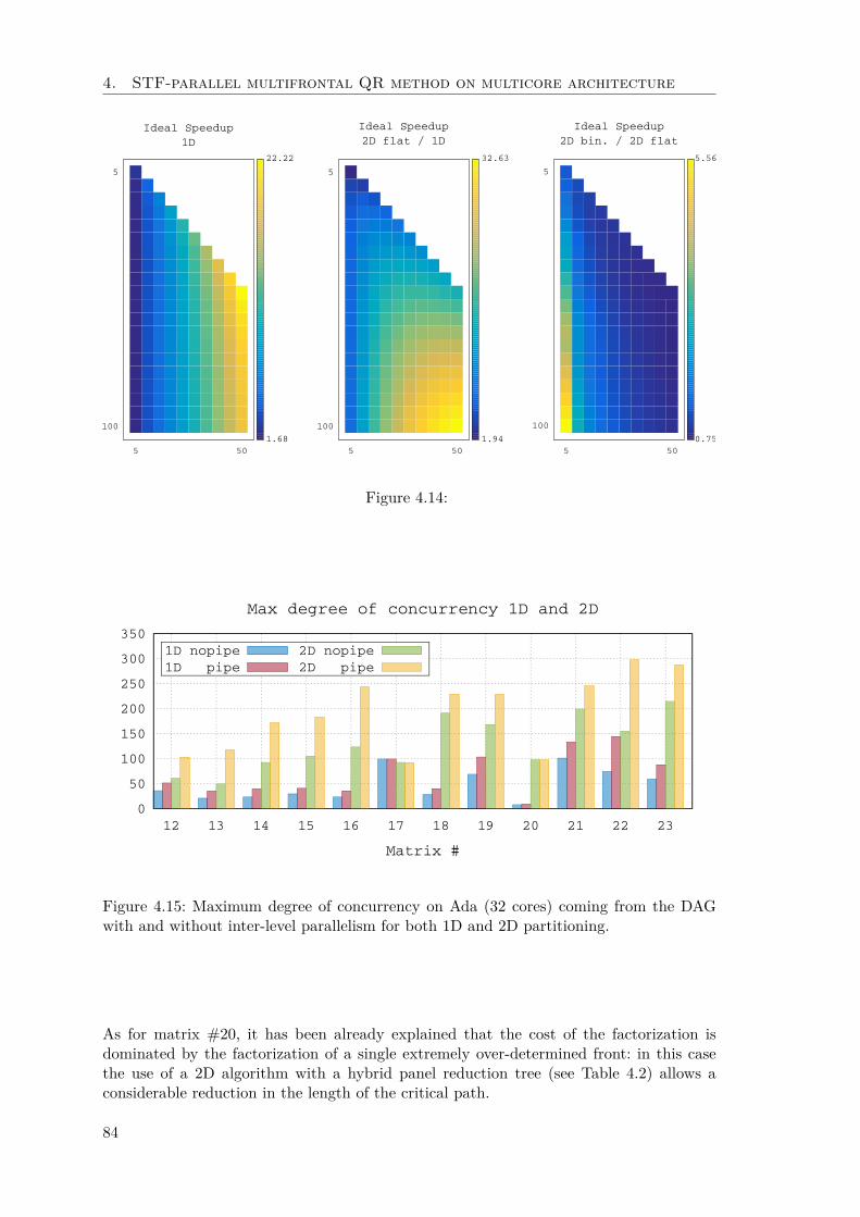
4. STF-parallel multifrontal QR method on multicore architecture

5 50

100

5

1.68

22.22

5 50

100

5

1.94

32.63

5 50

100

5

0.75

5.56

Ideal Speedup1D

Ideal Speedup2D flat / 1D

Ideal Speedup2D bin. / 2D flat

Figure 4.14:

0

50

100

150

200

250

300

350

12 13 14 15 16 17 18 19 20 21 22 23

Matrix #

Max degree of concurrency 1D and 2D

1D nopipe1D pipe

2D nopipe2D pipe

Figure 4.15: Maximum degree of concurrency on Ada (32 cores) coming from the DAGwith and without inter-level parallelism for both 1D and 2D partitioning.

As for matrix #20, it has been already explained that the cost of the factorization isdominated by the factorization of a single extremely over-determined front: in this casethe use of a 2D algorithm with a hybrid panel reduction tree (see Table 4.2) allows aconsiderable reduction in the length of the critical path.

84

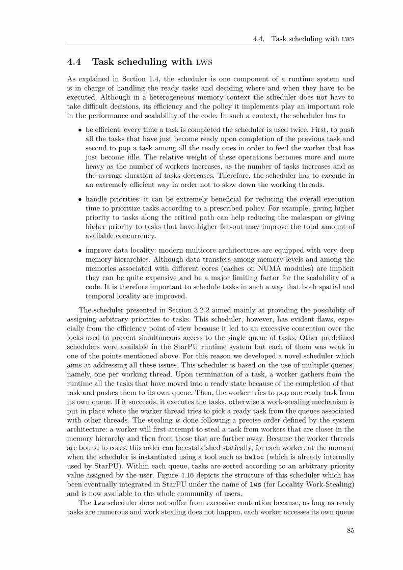
4.4. Task scheduling with lws

4.4 Task scheduling with lws

As explained in Section 1.4, the scheduler is one component of a runtime system andis in charge of handling the ready tasks and deciding where and when they have to beexecuted. Although in a heterogeneous memory context the scheduler does not have totake difficult decisions, its efficiency and the policy it implements play an important rolein the performance and scalability of the code. In such a context, the scheduler has to

• be efficient: every time a task is completed the scheduler is used twice. First, to pushall the tasks that have just become ready upon completion of the previous task andsecond to pop a task among all the ready ones in order to feed the worker that hasjust become idle. The relative weight of these operations becomes more and moreheavy as the number of workers increases, as the number of tasks increases and asthe average duration of tasks decreases. Therefore, the scheduler has to execute inan extremely efficient way in order not to slow down the working threads.

• handle priorities: it can be extremely beneficial for reducing the overall executiontime to prioritize tasks according to a prescribed policy. For example, giving higherpriority to tasks along the critical path can help reducing the makespan or givinghigher priority to tasks that have higher fan-out may improve the total amount ofavailable concurrency.

• improve data locality: modern multicore architectures are equipped with very deepmemory hierarchies. Although data transfers among memory levels and among thememories associated with different cores (caches on NUMA modules) are implicitthey can be quite expensive and be a major limiting factor for the scalability of acode. It is therefore important to schedule tasks in such a way that both spatial andtemporal locality are improved.

The scheduler presented in Section 3.2.2 aimed mainly at providing the possibility ofassigning arbitrary priorities to tasks. This scheduler, however, has evident flaws, espe-cially from the efficiency point of view because it led to an excessive contention over thelocks used to prevent simultaneous access to the single queue of tasks. Other predefinedschedulers were available in the StarPU runtime system but each of them was weak inone of the points mentioned above. For this reason we developed a novel scheduler whichaims at addressing all these issues. This scheduler is based on the use of multiple queues,namely, one per working thread. Upon termination of a task, a worker gathers from theruntime all the tasks that have moved into a ready state because of the completion of thattask and pushes them to its own queue. Then, the worker tries to pop one ready task fromits own queue. If it succeeds, it executes the tasks, otherwise a work-stealing mechanism isput in place where the worker thread tries to pick a ready task from the queues associatedwith other threads. The stealing is done following a precise order defined by the systemarchitecture: a worker will first attempt to steal a task from workers that are closer in thememory hierarchy and then from those that are further away. Because the worker threadsare bound to cores, this order can be established statically, for each worker, at the momentwhen the scheduler is instantiated using a tool such as hwloc (which is already internallyused by StarPU). Within each queue, tasks are sorted according to an arbitrary priorityvalue assigned by the user. Figure 4.16 depicts the structure of this scheduler which hasbeen eventually integrated in StarPU under the name of lws (for Locality Work-Stealing)and is now available to the whole community of users.

The lws scheduler does not suffer from excessive contention because, as long as readytasks are numerous and work stealing does not happen, each worker accesses its own queue

85

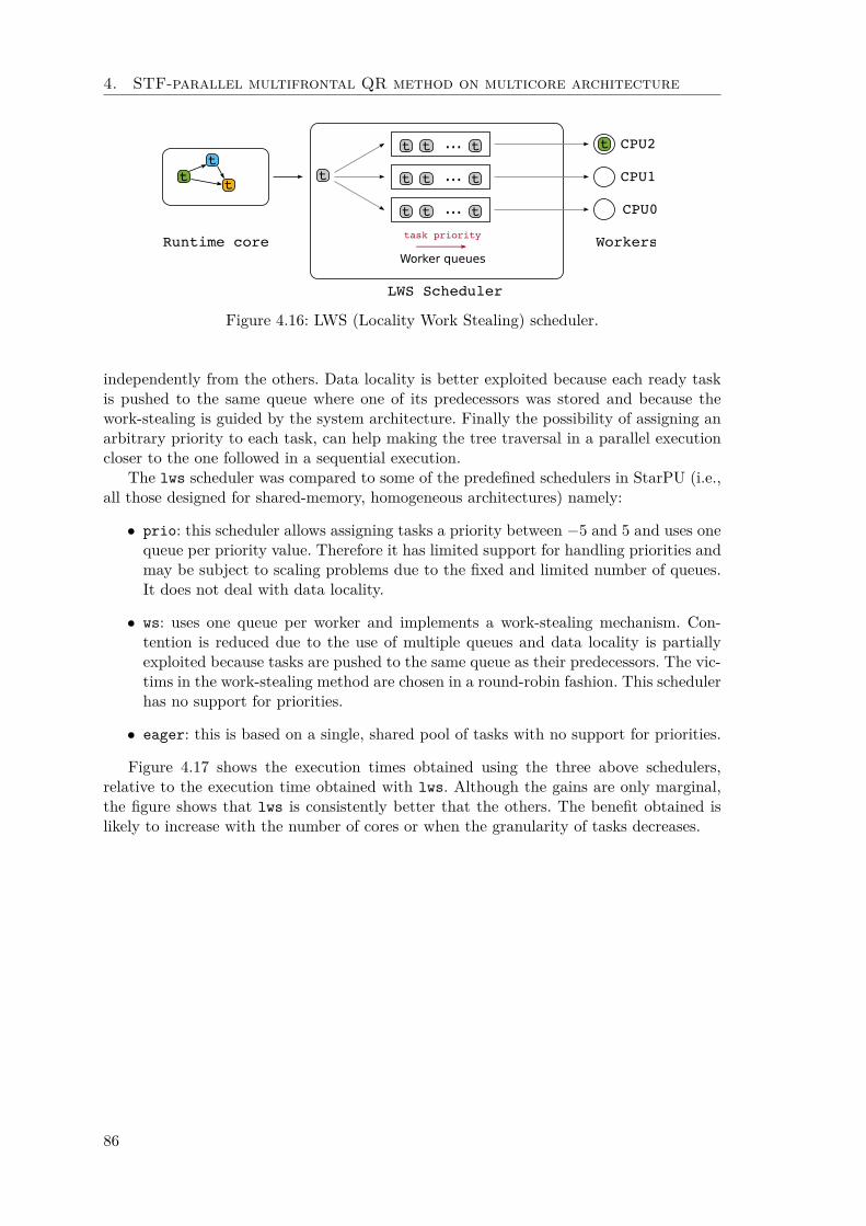
4. STF-parallel multifrontal QR method on multicore architecture

WorkersRuntime core

LWS Scheduler

Worker queues

CPU0

CPU2

CPU1t

t

t

task priority

t tt ...

t t tt ...

t tt ...

t

Figure 4.16: LWS (Locality Work Stealing) scheduler.

independently from the others. Data locality is better exploited because each ready taskis pushed to the same queue where one of its predecessors was stored and because thework-stealing is guided by the system architecture. Finally the possibility of assigning anarbitrary priority to each task, can help making the tree traversal in a parallel executioncloser to the one followed in a sequential execution.

The lws scheduler was compared to some of the predefined schedulers in StarPU (i.e.,all those designed for shared-memory, homogeneous architectures) namely:

• prio: this scheduler allows assigning tasks a priority between −5 and 5 and uses onequeue per priority value. Therefore it has limited support for handling priorities andmay be subject to scaling problems due to the fixed and limited number of queues.It does not deal with data locality.

• ws: uses one queue per worker and implements a work-stealing mechanism. Con-tention is reduced due to the use of multiple queues and data locality is partiallyexploited because tasks are pushed to the same queue as their predecessors. The vic-tims in the work-stealing method are chosen in a round-robin fashion. This schedulerhas no support for priorities.

• eager: this is based on a single, shared pool of tasks with no support for priorities.

Figure 4.17 shows the execution times obtained using the three above schedulers,relative to the execution time obtained with lws. Although the gains are only marginal,the figure shows that lws is consistently better that the others. The benefit obtained islikely to increase with the number of cores or when the granularity of tasks decreases.

86

4.4. Task scheduling with lws

0.8

1.0

1.2

12 13 14 15 16 17 18 19 20 21 22 23

Matrix #

Exection time relative to lws

prio

ws

eager

Figure 4.17: Factorization times obtained with pre-existing schedulers normalized to theone obtained with lws.

87

Chapter 5

Memory-aware multifrontalmethod

In this chapter we tackle the problem of controlling the memory consumption of the mul-tifrontal QR method and aim at imposing a constraint on the maximum memory usageduring the execution. The algorithm, based on the STF model and presented in the pre-vious chapter may lead to a large memory consumption as all the frontal matrices couldbe allocated immediately after the beginning of the execution. The strategy employed toreduce the memory consumption consists in trying to keep the traversal of the elimina-tion tree as close as possible to a postorder that minimizes the memory footprint in asequential execution. This approach, however, does not provide any means of controllingor predicting, in the parallel factorization, the memory consumption which can grow arbi-trarily. After a brief description of the memory behaviour for the multifrontal method, andreviewing the existing techniques for controlling its memory footprint, we propose a modi-fication of the STF algorithm capable of reliably controlling the memory consumption [S1]of a parallel factorization. Although, in principle, this technique may reduce the amountof available concurrency by limiting the use of tree parallelism, the experimental resultsreported below show that the actual reduction of performance is basically negligible.

5.1 Memory behavior of the multifrontal method

The memory needed to perform the multifrontal factorization (QR as well as LU or othertypes) is not statically allocated at once before the factorization begins but is allocatedand deallocated as the frontal matrices are activated and deactivated, as described inSection 1.2.3. Specifically, each activation task allocates all the memory needed to processa front; this memory can be split into two parts:

1. a persistent memory: once the frontal matrix is factorized, this part contains thefactor coefficients and, therefore, once allocated it is never freed, unless in an out-of-core execution (where factors are written on disk)1;

2. a temporary memory: this part contains the contribution block and is freed by thedeactivate task once the coefficients it contains have been assembled into the parentfront.

1In some other cases the factors can also be discarded as, for example, when the factorization is donefor computing the determinant of the matrix.

89

5. Memory-aware multifrontal method

As a result, the memory footprint of the multifrontal method in a sequential executionvaries greatly throughout the factorization. Starting at zero, it grows fast at the beginningas the first fronts are activated, it then goes up and down as fronts are activated anddeactivated until it reaches a maximum value (we refer to this value as the sequentialpeak) and eventually goes down towards the end of the factorization to the point wherethe only thing left in memory is the factors. The memory consumption varies depending onthe particular topological order followed for traversing the elimination tree and techniquesexist to determine the memory minimizing traversal for sequential executions as explainedin Section 5.2.

500

1000

1500

2000

2500

3000

3500

4000

50 100 150 200 250

Memory (MB)

Time (sec.)

Sequential

6 threads, no constraint

6 threads, Sequential*2.0

Figure 5.1: The memory profiles for matrix #12 for a sequential (in blue) and 6-threadedparallel factorization without memory constraint (in red) and with a constraint equal to2.0 times the sequential peak (in green).

Figure 5.1 shows, in the blue curve, the typical memory consumption profile of asequential multifrontal factorization; the data in this figure results from the factorizationof matrix #12. The memory footprint varies considerably throughout the factorizationand presents spikes immediately followed by sharp decreases; each spike corresponds tothe activation of a front whereas the following decrease corresponds to the deactivation ofits children once its assembly is completed.

It has to be noted that the use of tree parallelism normally increases the memoryconsumption of the multifrontal method simply because, in order to feed the workingprocesses, more work has to be generated and thus more fronts have to be activatedconcurrently. The memory consumption of the STF parallel code discussed so far can beconsiderably higher than the sequential peak (up to 3 times or more). This is due to thefact that the runtime system tries to execute tasks as soon as they are available and tothe fact that activation tasks are extremely fast and only depend upon each other; as aresult, all the fronts in the elimination tree are almost instantly allocated at the beginningof the factorization. This behaviour, moreover, is totally unpredictable because of the verydynamic execution model of the runtime system. This is depicted in Figure 5.1 with thered curve which shows the memory consumption for the case where our runtime basedSTF factorization is run with six threads; in this case the memory consumption is roughlyfive times higher than the sequential peak. Figure 5.2 shows the memory consumptionof the STF parallel code relative to the sequential code on a number of matrices whenexecuted on the Ada computer using 32 threads. As shown, in several cases the memoryincrease can be considerable, especially in the case where the factors are discarded due tothe fact that, in this case, the relative weight of the temporary memory is less.

90

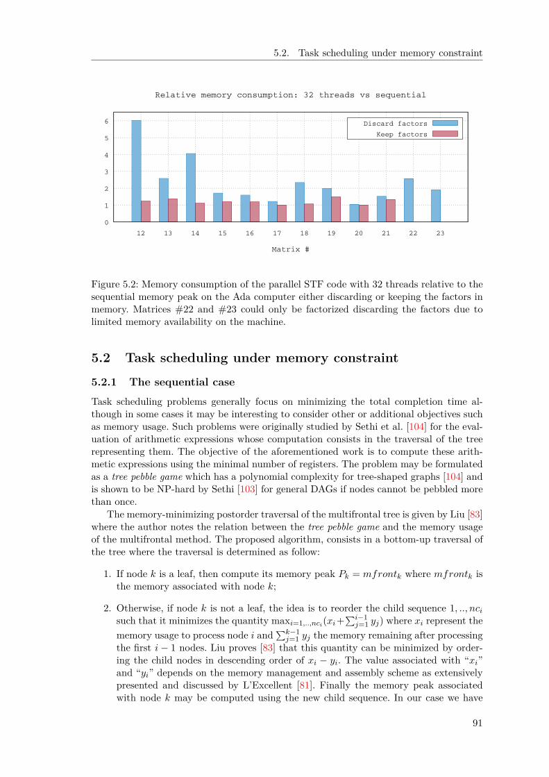
5.2. Task scheduling under memory constraint

0

1

2

3

4

5

6

12 13 14 15 16 17 18 19 20 21 22 23

Matrix #

Relative memory consumption: 32 threads vs sequential

Discard factors

Keep factors

Figure 5.2: Memory consumption of the parallel STF code with 32 threads relative to thesequential memory peak on the Ada computer either discarding or keeping the factors inmemory. Matrices #22 and #23 could only be factorized discarding the factors due tolimited memory availability on the machine.

5.2 Task scheduling under memory constraint

5.2.1 The sequential case

Task scheduling problems generally focus on minimizing the total completion time al-though in some cases it may be interesting to consider other or additional objectives suchas memory usage. Such problems were originally studied by Sethi et al. [104] for the eval-uation of arithmetic expressions whose computation consists in the traversal of the treerepresenting them. The objective of the aforementioned work is to compute these arith-metic expressions using the minimal number of registers. The problem may be formulatedas a tree pebble game which has a polynomial complexity for tree-shaped graphs [104] andis shown to be NP-hard by Sethi [103] for general DAGs if nodes cannot be pebbled morethan once.

The memory-minimizing postorder traversal of the multifrontal tree is given by Liu [83]where the author notes the relation between the tree pebble game and the memory usageof the multifrontal method. The proposed algorithm, consists in a bottom-up traversal ofthe tree where the traversal is determined as follow:

1. If node k is a leaf, then compute its memory peak Pk = mfrontk where mfrontk isthe memory associated with node k;

2. Otherwise, if node k is not a leaf, the idea is to reorder the child sequence 1, .., nci

such that it minimizes the quantity maxi=1,..,nci(xi+

∑i−1j=1 yj) where xi represent the

memory usage to process node i and∑k−1

j=1 yj the memory remaining after processingthe first i − 1 nodes. Liu proves [83] that this quantity can be minimized by order-ing the child nodes in descending order of xi − yi. The value associated with “xi”and “yi” depends on the memory management and assembly scheme as extensivelypresented and discussed by L’Excellent [81]. Finally the memory peak associatedwith node k may be computed using the new child sequence. In our case we have

91

5. Memory-aware multifrontal method

xi = max(Pi, mfrontk + Fk) and yj = cbj + Fj where cbj represents the memorysize of the contribution block for node j and Fj the size of factors in the subtreerooted at node j. In the case of an out-of-core execution the previous expressionsare changed into xi = max(Pi, mfrontk) and yj = cbj .

The optimal memory ordering is obtained using a depth-first traversal on the tree usingthe rearranged child sequences. The minimal memory usage for the sequential traversal ofthe elimination tree is given by the memory peak computed at the root node. Figure 5.3shows the variation of the memory usage during the factorization. The table on the rightside of the figure shows the memory consumption for a sequential execution where thetree is traversed in natural order which is a-b-c-d-e; the corresponding sequential peak isequal to 22 memory units. If we apply the above algorithm to the case of this figure thenwe find that the optimal memory traversal is b-c-d-a-e and the corresponding sequentialmemory peak is equals to 19 memory units.

a b c

d

e

(1,4)(1,4)

(8,1)

(3,0)

(2,1)

Task Memoryactivate(a) 3activate(b) 8activate(c) 13activate(d) 22

deactivate(b) 18deactivate(c) 14

activate(e) 17deactivate(a) 16deactivate(d) 15

Figure 5.3: The memory consumption (right) for a 5-nodes elimination tree (left) assuminga sequential traversal in natural order. Next to each node of the tree the two valuescorresponding to the factors (permanent) and the contribution block (temporary) sizes inmemory units.

Liu [82] observed that the postorder may not give the best memory usage among alltopological orders and proposes an algorithm to find the optimal memory topological orderfor a given tree. Motivated by tree structures emerging from the multifrontal factorization,Jacquelin et al. [74] give an alternative algorithm less costly for computing this memoryoptimal topological order. In practice, only postorders are considered because they providegood locality properties and, as pointed out by Jacquelin et al. [74], they often give optimaltraversal on trees coming from real applications.

5.2.2 The parallel case

The memory-minimization problem, extensively studied in sequential, has received littleattention in the parallel case. In recent work, Eyraud-Dubois et al. [50] show that theparallel variant of the pebble game is NP-complete and prove that there is no approximationalgorithm that can be designed to tackle the problem. They propose, instead, severalheuristics for scheduling task trees which aim at reducing the memory consumption of amultifrontal factorization2 in a shared memory, parallel setting. One of these heuristics,MemBookingInnerFirst is such that the parallel processing of the elimination tree

2Note that the problem is presented in a much more general form in their paper and not necessarilyrelated to the multifrontal factorization.

92

5.3. STF Memory-aware multifrontal method

can be achieved while respecting a prescribed memory bound. This is achieved through amemory reservation system; roughly speaking, when a tree node is activated not only is thememory needed for its processing allocated but the memory needed to process its parentis reserved. This reservation ensures that, when the parent node becomes ready, enoughmemory is available to process it; this prevents memory deadlocks (see the next section foran explanation of this issue). The authors validated experimentally this heuristic, as wellas the others, by simulating a rather simplistic shared memory parallelization scheme.

In the distributed memory parallel case, the memory issue is much harder to tacklebecause, not only has the memory consumption to be minimized but also it must bebalanced among the various nodes participating in the factorization. Sparse direct solverscommonly rely on the Proportional Mapping [92] method for distributing the work andmemory loads across the computer nodes. In this method all the resources assigned to anode of the elimination tree are partitioned into subsets whose size is relative to the weight(either in terms of memory or flops) of the child subtrees and each subset assigned to theroot of the corresponding child subtree. All the available resources are first mapped on theroot node and then the method works recursively until all the nodes of the tree have beenassigned some resources. The proportional mapping method mostly aims at balancing the(memory or computational) load of the processes but does not offer any guarantee on theoverall memory consumption. Indeed Rouet [97] proved that this method leads to a poormemory efficiency and scalability. A radically different approach, sometimes referred toas tree sequential mapping, consists in mapping all the available resources on every singlenode of the eliminations tree: as a result, the nodes of the tree are traversed sequentiallyand each node is processed in parallel using all the available resources. This approachachieves exactly the same memory consumption as in a sequential execution but suffersfrom very poor performance because tree parallelism is not used and because an excessiveamount of resources is allocated to fronts of potentially small size. In his PhD thesis, Rouet[97] refines a memory aware method that was first introduced by Agullo [1] and which mapsthe computational resources aiming at a good load balance under a prescribed memoryconstraint. The method attempts to apply the proportional mapping method but everytime a proportional mapping step is applied to a set of siblings it also checks whether theimposed memory constraint is respected within the corresponding subtrees. If it is not thecase, the method serializes the processing of the sibling subtrees by enforcing precedenceconstraints. Roughly speaking, the method tries to apply proportional mapping as muchas possible but whenever this leads to a violation of the memory constraints it locallyreverts to tree sequential mapping.

5.3 STF Memory-aware multifrontal method

This section proposes a method for limiting the memory consumption of parallel executionsof our STF code by forcing it to respect a prescribed memory constraint which has to beequal to or bigger than the sequential peak. This technique shares commonalities withthe MemBookingInnerFirst heuristic proposed by Eyraud-Dubois et al. [50]. On theother hand, whereas Eyraud-Dubois et al. [51] only consider the theoretical problem, thepresent study proposes a new and robust algorithm to ensure that the imposed memoryconstraint is guaranteed while allowing a maximum amount of concurrency on shared-memory multicore architectures. In the remainder of this section we assume that the treetraversal order is fixed and we do not tackle the problem of finding a different traversalthat minimizes the memory footprint.

We rely on the STF model to achieve this objective with a relatively simple algorithm.

93

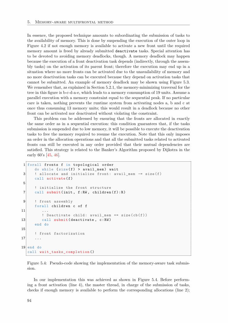
5. Memory-aware multifrontal method

In essence, the proposed technique amounts to subordinating the submission of tasks tothe availability of memory. This is done by suspending the execution of the outer loop inFigure 4.2 if not enough memory is available to activate a new front until the requiredmemory amount is freed by already submitted deactivate tasks. Special attention hasto be devoted to avoiding memory deadlocks, though. A memory deadlock may happenbecause the execution of a front deactivation task depends (indirectly, through the assem-bly tasks) on the activation of its parent front; therefore the execution may end up in asituation where no more fronts can be activated due to the unavailability of memory andno more deactivation tasks can be executed because they depend on activation tasks thatcannot be submitted. An example of memory deadlock may be shown using Figure 5.3.We remember that, as explained in Section 5.2.1, the memory-minimizing traversal for thetree in this figure is b-c-d-a-e, which leads to a memory consumption of 19 units. Assume aparallel execution with a memory constraint equal to the sequential peak. If no particularcare is taken, nothing prevents the runtime system from activating nodes a, b and c atonce thus consuming 13 memory units; this would result in a deadlock because no otherfront can be activated nor deactivated without violating the constraint.

This problem can be addressed by ensuring that the fronts are allocated in exactlythe same order as in a sequential execution: this condition guarantees that, if the taskssubmission is suspended due to low memory, it will be possible to execute the deactivationtasks to free the memory required to resume the execution. Note that this only imposesan order in the allocation operations and that all the submitted tasks related to activatedfronts can still be executed in any order provided that their mutual dependencies aresatisfied. This strategy is related to the Banker’s Algorithm proposed by Dijkstra in theearly 60’s [45, 46].

1 forall fronts f in topological order

do while (size(f) > avail_mem ) wait

3 ! allocate and initialize front: avail_mem -= size(f)

call activate (f)

5

! initialize the front structure

7 call submit (init , f:RW , children (f):R)

9 ! front assembly

forall children c of f

11 ...

! Deactivate child: avail_mem += size(cb(f))

13 call submit (deactivate , c:RW)

end do

15

! front factorization

17 ...

19 end do

call wait_tasks_completion ()

Figure 5.4: Pseudo-code showing the implementation of the memory-aware task submis-sion.

In our implementation this was achieved as shown in Figure 5.4. Before perform-ing a front activation (line 4), the master thread, in charge of the submission of tasks,checks if enough memory is available to perform the corresponding allocations (line 2);

94

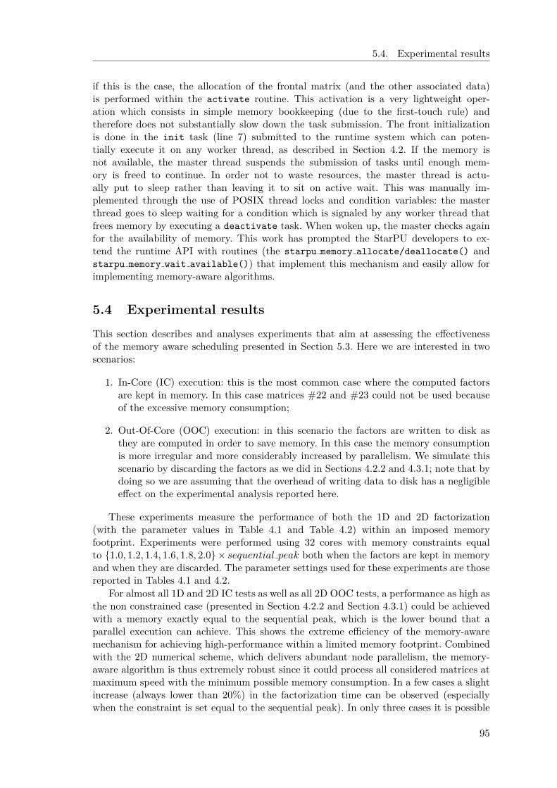
5.4. Experimental results

if this is the case, the allocation of the frontal matrix (and the other associated data)is performed within the activate routine. This activation is a very lightweight oper-ation which consists in simple memory bookkeeping (due to the first-touch rule) andtherefore does not substantially slow down the task submission. The front initializationis done in the init task (line 7) submitted to the runtime system which can poten-tially execute it on any worker thread, as described in Section 4.2. If the memory isnot available, the master thread suspends the submission of tasks until enough mem-ory is freed to continue. In order not to waste resources, the master thread is actu-ally put to sleep rather than leaving it to sit on active wait. This was manually im-plemented through the use of POSIX thread locks and condition variables: the masterthread goes to sleep waiting for a condition which is signaled by any worker thread thatfrees memory by executing a deactivate task. When woken up, the master checks againfor the availability of memory. This work has prompted the StarPU developers to ex-tend the runtime API with routines (the starpu memory allocate/deallocate() andstarpu memory wait available()) that implement this mechanism and easily allow forimplementing memory-aware algorithms.

5.4 Experimental results

This section describes and analyses experiments that aim at assessing the effectivenessof the memory aware scheduling presented in Section 5.3. Here we are interested in twoscenarios:

1. In-Core (IC) execution: this is the most common case where the computed factorsare kept in memory. In this case matrices #22 and #23 could not be used becauseof the excessive memory consumption;

2. Out-Of-Core (OOC) execution: in this scenario the factors are written to disk asthey are computed in order to save memory. In this case the memory consumptionis more irregular and more considerably increased by parallelism. We simulate thisscenario by discarding the factors as we did in Sections 4.2.2 and 4.3.1; note that bydoing so we are assuming that the overhead of writing data to disk has a negligibleeffect on the experimental analysis reported here.

These experiments measure the performance of both the 1D and 2D factorization(with the parameter values in Table 4.1 and Table 4.2) within an imposed memoryfootprint. Experiments were performed using 32 cores with memory constraints equalto {1.0, 1.2, 1.4, 1.6, 1.8, 2.0} × sequential peak both when the factors are kept in memoryand when they are discarded. The parameter settings used for these experiments are thosereported in Tables 4.1 and 4.2.

For almost all 1D and 2D IC tests as well as all 2D OOC tests, a performance as high asthe non constrained case (presented in Section 4.2.2 and Section 4.3.1) could be achievedwith a memory exactly equal to the sequential peak, which is the lower bound that aparallel execution can achieve. This shows the extreme efficiency of the memory-awaremechanism for achieving high-performance within a limited memory footprint. Combinedwith the 2D numerical scheme, which delivers abundant node parallelism, the memory-aware algorithm is thus extremely robust since it could process all considered matrices atmaximum speed with the minimum possible memory consumption. In a few cases a slightincrease (always lower than 20%) in the factorization time can be observed (especiallywhen the constraint is set equal to the sequential peak). In only three cases it is possible

95

5. Memory-aware multifrontal method

to observe a smooth decrease of the factorization time as the constraint on the memoryconsumption is relaxed: these are the OOC, 1D factorization of matrices #12, #14 and#18.

To explain this extreme efficiency, we performed the following analysis. As explained inSection 5.3, prior to activating a front, the master thread checks whether enough memoryis available to achieve this operation. If it is not the case, the master thread is put tosleep and later woken up as soon as one deactivate task is executed; at this time themaster thread checks again for the availability of memory. The master thread stays in thisloop until enough deactivation tasks have been executed to free up the memory neededto proceed with the next front activation. Every time the master thread was suspendedor resumed we recorded the time stamp and the number of ready tasks (i.e., those whosedependencies were all satisfied).

Figure 5.6 shows the collected data for matrix #12 with an imposed memory consump-tion equal to the sequential peak, in the OOC case using both the 1D (left) and 2D (right)methods. In this figure, each (x, y) point means that at time x the master thread wassuspended or resumed and that, at that time, y tasks where ready for execution or beingexecuted. The width of each graph shows the execution time of the memory constrainedfactorization whereas the vertical dashed line shows the execution time when no limit onthe memory consumption is imposed. The figure leads to the following observations:

• in both the 1D and 2D factorizations, the number of ready tasks falls, at some point,below the number of available cores (the horizontal, solid line); this lack of tasks isresponsible for a longer execution time with respect to the unconstrained case.

• in the 1D factorization this lack of tasks is more evident; this can be explainedby the fact that the 1D method delivers much lower concurrency than the 2D oneand therefore, suspending the submission of tasks may lead more quickly to threadstarvation. As a result, the difference in the execution times of the constrained andunconstrained executions is more evident in the 1D factorization.

For all other tests, either the number of tasks is always (much) higher than the numberof workers or the tasks submission is never (or almost never) interrupted due to the lackof memory; as a result, no relevant performance degradation was observed with respect tothe case where no memory constraint is imposed. This behavior mainly results from twoproperties of the multifrontal QR factorization:

1. the size of the contribution blocks is normally very small compared to the size offactors, especially in the case where frontal matrices are overdetermined;

2. the size of a front is always greater than or equal to the sum of the sizes of all thecontribution blocks associated with its children (because in the assembly operation,contribution blocks are not summed to each other but stacked).

As a result, in the sequential multifrontal QR factorization, the memory consumptiongrows almost monotonically and in most cases the sequential peak is achieved on the rootnode or very close to it. For this reason, when the tasks submission is interrupted in amemory-constrained execution, a large portion of the elimination tree has already beensubmitted and the number of available tasks is considerably larger than the number ofworking threads. Other types of multifrontal factorizations (LU , for instance) are likely tobe more sensitive to the memory constraint because they do not possess the two propertiesdescribed above. By the same token, it is reasonable to expect that imposing a memory

96

5.4. Experimental results

0.8

1.0

1.2

1.4

1.6

12 13 14 15 16 17 18 19 20 21 22 23

Matrix #

Relative time constrained vs not. 2D, discard

1.0

1.2

1.4

1.6

1.8

2.0

0.8

1.0

1.2

1.4

1.6

12 13 14 15 16 17 18 19 20 21 22 23

Matrix #

Relative time constrained vs not. 2D, keep

1.0

1.2

1.4

1.6

1.8

2.0

0.8

1.0

1.2

1.4

1.6

12 13 14 15 16 17 18 19 20 21 22 23

Matrix #

Relative time constrained vs not. 1D, discard

1.0

1.2

1.4

1.6

1.8

2.0

0.8

1.0

1.2

1.4

1.6

12 13 14 15 16 17 18 19 20 21 22 23

Matrix #

Relative time constrained vs not. 1D, keep

1.0

1.2

1.4

1.6

1.8

2.0

Figure 5.5: Memory-constrained factorization times relative to the unconstrained execu-tion for the 2D and 1D methods either discarding (OOC) or keeping (IC) the factors inmemory. Matrices #22 and #23 could only be factorized discarding the factors (OOC)due to limited memory availability on the machine.

97

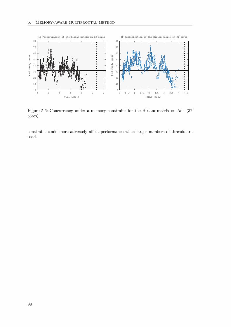
5. Memory-aware multifrontal method

0

10

20

30

40

50

60

70

80

0 1 2 3 4 5 6

# of ready tasks

Time (sec.)

1D Factorization of the Hirlam matrix on 32 cores

0

10

20

30

40

50

60

70

80

0 0.5 1 1.5 2 2.5 3 3.5 4 4.5

# of ready tasks

Time (sec.)

2D Factorization of the Hirlam matrix on 32 cores

Figure 5.6: Concurrency under a memory constraint for the Hirlam matrix on Ada (32cores).

constraint could more adversely affect performance when larger numbers of threads areused.

98

Chapter 6

STF-parallel multifronatal QRmethod on heterogeneousarchitecture

In this chapter we present the implementation of a multifrontal method for heterogeneousarchitectures such as GPU-accelerated multicore systems. The implementation presentedin Chapter 4 constitutes the basis for this work and as we showed in the multicore case,the runtime system facilitates the development of such algorithms in the context of hetero-geneous systems. First of all, the runtime system is capable of handling the data transfersand managing the data consistency across the architecture then, by providing kernels spe-cific to accelerators, it is able to execute tasks on accelerators following a given schedulingstrategy. We show in this chapter that solely providing the kernels for accelerator is notsufficient to efficiently exploit the potential performance of accelerator based systems andwe propose frontal matrix partitioning and scheduling strategies to attain good perfor-mance on such machines. In addition using the performance analysis approach presentedin Chapter 2 we are capable of evaluating how well we are exploiting the acceleratedarchitectures on which we performed our experiments.

6.1 Frontal matrices partitioning schemes

Finding frontal matrix partitioning strategies that allows an efficient exploitation of bothCPU and GPU resources constitutes one of the main challenges in implementing a mul-tifrontal method for GPU-accelerated multicore systems. This results from the fact thatGPUs, which are potentially able to deliver much higher performance than CPUs, re-quire coarse granularity operations to achieve peak performance while a CPU reaches itspeak with relatively small granularity tasks. The approach presented in Section 4.2, wherefrontal matrices are uniformly partitioned into small size block-columns, could be readilyported to GPU-accelerated platforms by simply providing GPU implementations for thevarious tasks to the StarPU runtime system. This, however, would result in an unsatis-factory performance because, due to the fine granularity of tasks, only a small fraction ofthe GPU performance could be used. This front partitioning strategy, which we refer toas fine-grain partitioning, shown in Figure 6.1(a), is not suited to heterogeneous architec-tures despite being able to deliver sufficient concurrency to feed both the CPU cores andthe GPU and reduce idle times on all the resources. A radically different approach is whatwe refer to as coarse-grain partitioning (Figure 6.1(b)), where fine-grained panel tasks areexecuted on CPU and large-grain (as large as possible) update tasks are performed on

99

6. STF-parallel multifronatal QR method on heterogeneous

architecture

GPU. This corresponds to the algorithm used in the MAGMA package [9] and aims atobtaining the best acceleration of computationally intensive tasks on the GPU. In orderto keep the GPU constantly busy, static scheduling is used that allows the overlapping ofGPU and CPU computation thanks to a depth-1 lookahead technique; this is achieved bysplitting the trailing submatrix update into two separate tasks of, respectively, fine andcoarse granularity. This second approach clearly incurs the opposite problem than the onewe face with the fine-grain partitioning: despite being able to maximize the efficiency ofGPU operations with respect to the problem size, it severely limits the amount of nodeparallelism as well as of inter-level parallelism (see Section 1.7.1 and 4.2.3) and thereforeleads to resource (especially CPUs) starvation.

Panel

Update

nbcpu

(a) Fine-grain parti-tioning.

Panel

Update

nbcpu

(b) Coarse-grain parti-tioning.

nbgpu

nbcpu

(c) Hierarchical-grainpartitioning.

Figure 6.1: Partitioning schemes.

In order to take advantage of the fine and coarse-grain approaches and to overcomethe limitations of both, we developed a hierarchical partitioning of fronts (Figure 6.1(c))which is similar to the approach proposed by Wu et al. [116] and corresponds to a trade-offbetween parallelism and GPU kernel efficiency with task granularity suited for both typesof resources. The front is first partitioned into coarse grain block-columns, referred to asouter block-columns, of width nbGPU suitable for GPU computation (this happens at themoment when the front is activated) and then each outer block-column is dynamicallyre-partitioned into inner block-columns of width nbCPU appropriate for the CPU only im-mediately before being factorized. This is achieved through dedicated partitioning taskswhich are subject to dependencies with respect to the other, previously submitted, tasksthat operate on the same data. When these dependencies are satisfied, StarPU ensuresthat the block being re-partitioned is in a consistent state, in case there are multiple copiesof it. Furthermore, StarPU ensures that the partitioning is performed in a logical fashion:no actual copy is performed and there is no extra data allocated. The partitioning is doneusing two tasks: partition and unpartition. In order to partition a data i representedby the handle f(i) into n pieces, it is necessary to declare the handles associated with thesub-data f(i,1)..f(i,n). The partition task takes as input the data to be partitioned

100

6.1. Frontal matrices partitioning schemes

forall outer panels o_p =1... o_n in f

2 ! partition (outer) block column f(o_p) into

! i_n inner block columns f(o_p ,1) .. f(o_p ,i_n)

4 call submit (partition , f(o_p):R, f(o_p ,1):W... f(o_p ,i_n):W)

6 forall inner panels i_p =1.. i_n

! panel reduction of inner block column i_p

8 call submit (_geqrt , f(i_p):RW)

forall inner blockcolumns i_u=i_p +1.. i_n in f(o_p)

10 ! update (inner) column in_u with panel i_p

call submit (_gemqrt , f(i_p):R, f(i_u):RW)

12 end do

14 forall outer blockcolumns o_u=o_p +1.. o_n

! update outer block column o_u with panel i_p

16 call submit (_gemqrt , f(i_p):R,f(o_u):RW)

end do

18 end do

20 ! unpartition (outer ) block column

call submit ( unpartition , f(o_p ,1):R...f(o_p ,i_n):R, f(o_p):W)

22 end do

Figure 6.2: STF code for the hierarchical QR factorization of frontal matrices.

forall panels p=1...n in f

2

! partition trailing submatrix

4 call submit (partition , f(p,tr):R, f(p,bc):W, f(p+1,tr):W)

6 ! panel reduction of block column p

call submit (_geqrt , f(p,bc):RW)

8

! update trailing submatrix p+1 with panel p

10 call submit (_gemqrt , f(p+1,tr):RW)

12 ! unpartition trailing submatrix

call submit ( unpartition , f(p,bc):R, f(p+1,tr):R, f(p,tr):W)

14

end do

Figure 6.3: STF code for the coarse QR factorization of frontal matrices.

101

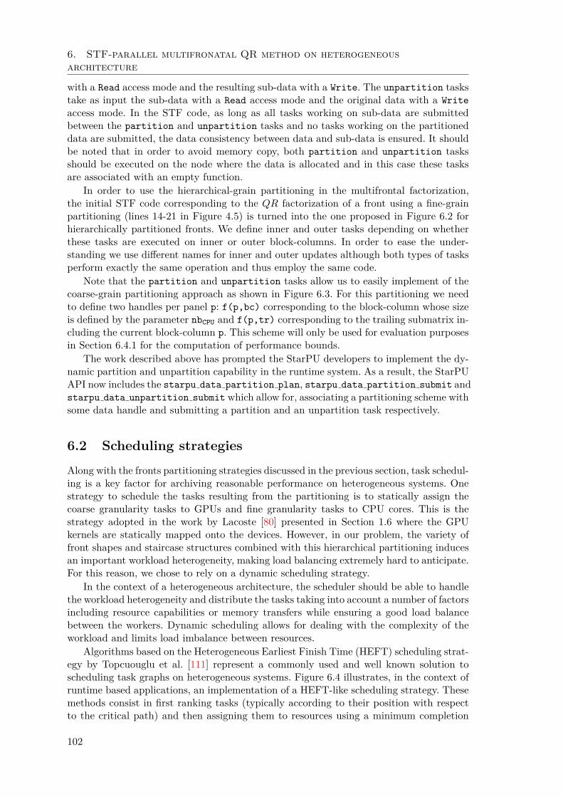
6. STF-parallel multifronatal QR method on heterogeneous

architecture

with a Read access mode and the resulting sub-data with a Write. The unpartition taskstake as input the sub-data with a Read access mode and the original data with a Write

access mode. In the STF code, as long as all tasks working on sub-data are submittedbetween the partition and unpartition tasks and no tasks working on the partitioneddata are submitted, the data consistency between data and sub-data is ensured. It shouldbe noted that in order to avoid memory copy, both partition and unpartition tasksshould be executed on the node where the data is allocated and in this case these tasksare associated with an empty function.

In order to use the hierarchical-grain partitioning in the multifrontal factorization,the initial STF code corresponding to the QR factorization of a front using a fine-grainpartitioning (lines 14-21 in Figure 4.5) is turned into the one proposed in Figure 6.2 forhierarchically partitioned fronts. We define inner and outer tasks depending on whetherthese tasks are executed on inner or outer block-columns. In order to ease the under-standing we use different names for inner and outer updates although both types of tasksperform exactly the same operation and thus employ the same code.

Note that the partition and unpartition tasks allow us to easily implement of thecoarse-grain partitioning approach as shown in Figure 6.3. For this partitioning we needto define two handles per panel p: f(p,bc) corresponding to the block-column whose sizeis defined by the parameter nbCPU and f(p,tr) corresponding to the trailing submatrix in-cluding the current block-column p. This scheme will only be used for evaluation purposesin Section 6.4.1 for the computation of performance bounds.

The work described above has prompted the StarPU developers to implement the dy-namic partition and unpartition capability in the runtime system. As a result, the StarPUAPI now includes the starpu data partition plan, starpu data partition submit andstarpu data unpartition submit which allow for, associating a partitioning scheme withsome data handle and submitting a partition and an unpartition task respectively.

6.2 Scheduling strategies

Along with the fronts partitioning strategies discussed in the previous section, task schedul-ing is a key factor for archiving reasonable performance on heterogeneous systems. Onestrategy to schedule the tasks resulting from the partitioning is to statically assign thecoarse granularity tasks to GPUs and fine granularity tasks to CPU cores. This is thestrategy adopted in the work by Lacoste [80] presented in Section 1.6 where the GPUkernels are statically mapped onto the devices. However, in our problem, the variety offront shapes and staircase structures combined with this hierarchical partitioning inducesan important workload heterogeneity, making load balancing extremely hard to anticipate.For this reason, we chose to rely on a dynamic scheduling strategy.

In the context of a heterogeneous architecture, the scheduler should be able to handlethe workload heterogeneity and distribute the tasks taking into account a number of factorsincluding resource capabilities or memory transfers while ensuring a good load balancebetween the workers. Dynamic scheduling allows for dealing with the complexity of theworkload and limits load imbalance between resources.

Algorithms based on the Heterogeneous Earliest Finish Time (HEFT) scheduling strat-egy by Topcuouglu et al. [111] represent a commonly used and well known solution toscheduling task graphs on heterogeneous systems. Figure 6.4 illustrates, in the context ofruntime based applications, an implementation of a HEFT-like scheduling strategy. Thesemethods consist in first ranking tasks (typically according to their position with respectto the critical path) and then assigning them to resources using a minimum completion

102

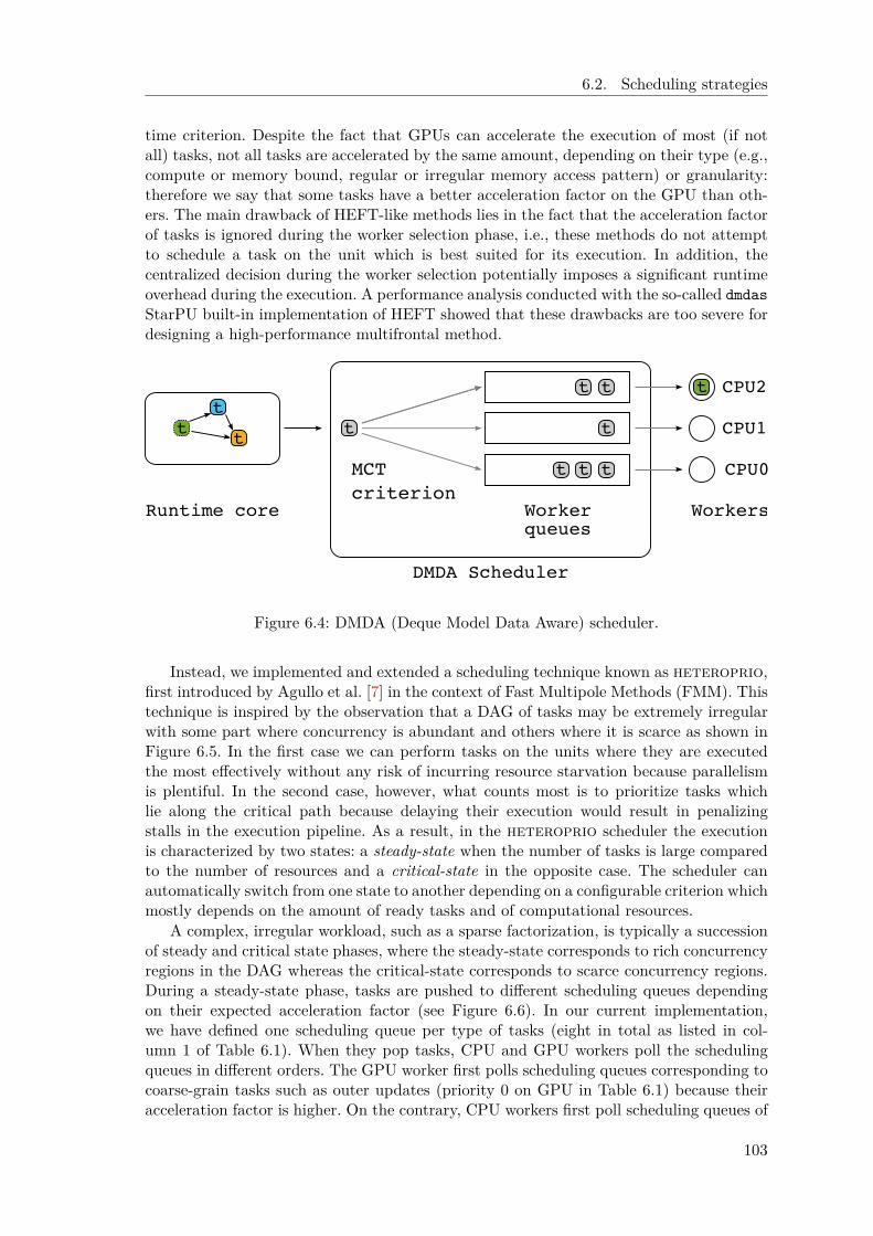
6.2. Scheduling strategies

time criterion. Despite the fact that GPUs can accelerate the execution of most (if notall) tasks, not all tasks are accelerated by the same amount, depending on their type (e.g.,compute or memory bound, regular or irregular memory access pattern) or granularity:therefore we say that some tasks have a better acceleration factor on the GPU than oth-ers. The main drawback of HEFT-like methods lies in the fact that the acceleration factorof tasks is ignored during the worker selection phase, i.e., these methods do not attemptto schedule a task on the unit which is best suited for its execution. In addition, thecentralized decision during the worker selection potentially imposes a significant runtimeoverhead during the execution. A performance analysis conducted with the so-called dmdas

StarPU built-in implementation of HEFT showed that these drawbacks are too severe fordesigning a high-performance multifrontal method.

WorkersRuntime core

CPU0

CPU2

CPU1

tt

t

tt t

DMDA Scheduler

Worker

queues

t

MCT

criterion

t

t

t

t

Figure 6.4: DMDA (Deque Model Data Aware) scheduler.

Instead, we implemented and extended a scheduling technique known as heteroprio,first introduced by Agullo et al. [7] in the context of Fast Multipole Methods (FMM). Thistechnique is inspired by the observation that a DAG of tasks may be extremely irregularwith some part where concurrency is abundant and others where it is scarce as shown inFigure 6.5. In the first case we can perform tasks on the units where they are executedthe most effectively without any risk of incurring resource starvation because parallelismis plentiful. In the second case, however, what counts most is to prioritize tasks whichlie along the critical path because delaying their execution would result in penalizingstalls in the execution pipeline. As a result, in the heteroprio scheduler the executionis characterized by two states: a steady-state when the number of tasks is large comparedto the number of resources and a critical-state in the opposite case. The scheduler canautomatically switch from one state to another depending on a configurable criterion whichmostly depends on the amount of ready tasks and of computational resources.

A complex, irregular workload, such as a sparse factorization, is typically a successionof steady and critical state phases, where the steady-state corresponds to rich concurrencyregions in the DAG whereas the critical-state corresponds to scarce concurrency regions.During a steady-state phase, tasks are pushed to different scheduling queues dependingon their expected acceleration factor (see Figure 6.6). In our current implementation,we have defined one scheduling queue per type of tasks (eight in total as listed in col-umn 1 of Table 6.1). When they pop tasks, CPU and GPU workers poll the schedulingqueues in different orders. The GPU worker first polls scheduling queues corresponding tocoarse-grain tasks such as outer updates (priority 0 on GPU in Table 6.1) because theiracceleration factor is higher. On the contrary, CPU workers first poll scheduling queues of

103

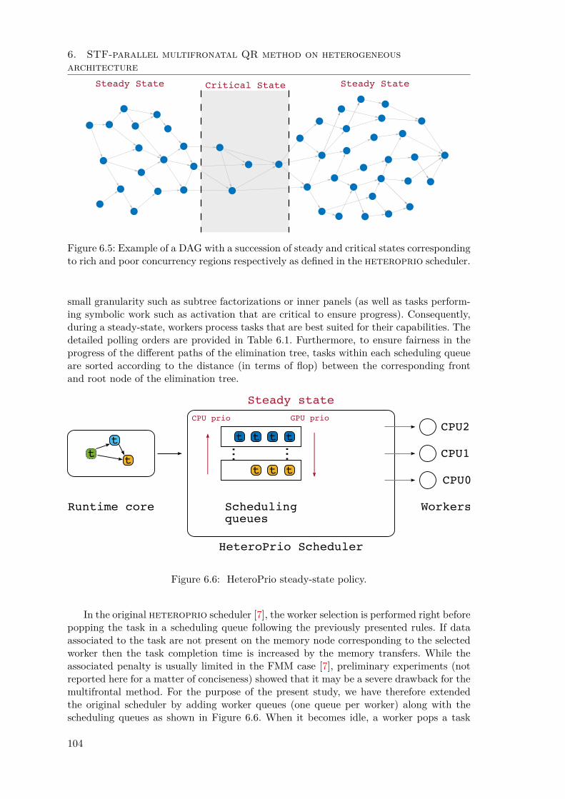
6. STF-parallel multifronatal QR method on heterogeneous

architecture

Steady State Critical State Steady State

Figure 6.5: Example of a DAG with a succession of steady and critical states correspondingto rich and poor concurrency regions respectively as defined in the heteroprio scheduler.

small granularity such as subtree factorizations or inner panels (as well as tasks perform-ing symbolic work such as activation that are critical to ensure progress). Consequently,during a steady-state, workers process tasks that are best suited for their capabilities. Thedetailed polling orders are provided in Table 6.1. Furthermore, to ensure fairness in theprogress of the different paths of the elimination tree, tasks within each scheduling queueare sorted according to the distance (in terms of flop) between the corresponding frontand root node of the elimination tree.

WorkersRuntime core

CPU0

CPU2

CPU1

t

HeteroPrio Scheduler

ttt

t t t

...

...

Scheduling

queues

CPU prio GPU prio

Steady state

t

t

t

Figure 6.6: HeteroPrio steady-state policy.

In the original heteroprio scheduler [7], the worker selection is performed right beforepopping the task in a scheduling queue following the previously presented rules. If dataassociated to the task are not present on the memory node corresponding to the selectedworker then the task completion time is increased by the memory transfers. While theassociated penalty is usually limited in the FMM case [7], preliminary experiments (notreported here for a matter of conciseness) showed that it may be a severe drawback for themultifrontal method. For the purpose of the present study, we have therefore extendedthe original scheduler by adding worker queues (one queue per worker) along with thescheduling queues as shown in Figure 6.6. When it becomes idle, a worker pops a task

104

6.3. Implementation details

from its worker queue and then fills it up again by picking a new task from the schedulingqueues through the polling procedure described above. The data associated with tasks ina worker queue can be automatically prefetched on the corresponding memory node whilethe corresponding worker is executing other tasks. If the size of the worker queues is toohigh, a task may be assigned to a worker much earlier than its actual execution, whichmay result in a sub-optimal choice. Therefore, because no additional benefit was observedbeyond this value, we set this size to two in our experiments.

Scheduling queues Steady-state Critical-stateCPU GPU CPU GPU

activate 0 - 0 -assemble 7 - 5 -deactivate 1 - 1 -do subtree 2 2 2 0part./unpart. 3 - 3 -inner panel 4 - 4 -inner update 5 1 6 1outer update 6 0 7 2

Table 6.1: Scheduling queues and polling orders in HeteroPrio.

When the number of tasks becomes low (with respect to a fixed threshold which isset depending on the amount of computational power of the platform), the schedulingalgorithm switches to critical-state. CPU and GPU workers cooperate to process criticaltasks as early as possible in order to produce new ready tasks quickly. For instance, becauseouter updates are less likely to be on the critical path, the GPU worker will select themlast in spite of their high acceleration factor. The last two columns of Table 6.1 provide thecorresponding polling order. Additionally, in this state, CPU workers are allowed to selecta task only if its expected completion time does not exceed the total completion timeof the tasks remaining in the GPU worker queue. This extra rule prevents CPU workersfrom selecting all the few available tasks and leaving the GPU idle whereas it could havefinished processing them all quickly.

6.3 Implementation details

In the proposed implementation we use, in addition to the CPU kernels, two GPU kernels:the gemqrt kernel corresponding to the update operation and the do subtree kernel forthe factorization of subtrees whose root node is on the layer resulting from the logicaltree pruning as explained in section 1.7.2. The gemqrt on GPU is performed using themagma {s,d,z,c}larfb gpu routine from the MAGMA package [9] which is the equivalentto the larfb kernel for CPUs. In order to exploit computationally intensive kernels andavoid irregularities in the memory access pattern of the factors V that are applied toa block-column, this kernel performs extra computations on the elements on the upper-right corner of the matrix V . This strategy allows us to obtain better kernel performanceat the cost of additional flops for this operation. Note, also, that this routine is notcapable of exploiting, internally, the staircase structure of the panel. The do subtree ona GPU consists in a sequential tree traversal where fronts are initialized and assembledon the CPU and factorized on the GPU. For this factorization operation, a coarse-grainpartitioning is used similarly to the magma {s,d,c,z}geqrf routine from MAGMA. This

105

6. STF-parallel multifronatal QR method on heterogeneous

architecture

routine however cannot be used is our case because of the staircase structure of frontalmatrices. Instead, we developed a routine called {s,d,c,z}geqrf stair gpu performingcoarse-grain factorization of a front using the same mapping of tasks as the MAGMAroutine magma {s,d,z,c}geqrf and capable of exploiting the frontal matrices staircasestructure.

As explained in Section 1.4.2.1, when tasks are scheduled on a GPU worker StarPUautomatically handles the memory transfers of associated data on the GPU memory node.For the gemqrt tasks with respect to a panel operation, the V and T matrix resulting fromthe panel and the C block-column to be updated are associated with the tasks and thus willbe automatically transferred to the GPU if necessary. In the case of a do subtree the CPU-GPU memory transfers are performed by {s,d,c,z}geqrf stair gpu kernels. The datamanipulated in the task are not associated with the task in order to prevent the runtimesystem from transferring the whole subtree to the GPU before the execution of a task.Instead, the data manipulated in a do subtree task are represented by a symbolic handleallowing a declaration of the dependencies with the tasks depending on the do subtree

tasks.

6.4 Experimental results

6.4.1 Performance and analysis

We tested the previously presented implementation on a subset of the test matrices inTable 1.1; the experiments were done on one node of the Sirocco cluster presented inSection 1.9.1. In this experimental study we evaluate the performance of the STF par-allel multifrontal QR method on heterogeneous architectures using the frontal matricespartitioning and scheduling strategies described above. We first tested the parallel codeusing CPU workers only and then we added one GPU worker. For the CPU only ex-periments we use the fine-grain (i.e. block-column) partitioning presented above and inSection 4.2. As explained in Section 4.2.2 the performance of the parallel factorizationusing a block-column partitioning depends on several parameters. In the fine-grain casethese parameters are nb which impacts the concurrency generated in the DAG and theinner block size ib which affects the efficiency of elementary BLAS kernels and determinesthe global amount of flop performed during the factorization. Finding the optimal param-eters for this is extremely difficult because it depends on a great number of factors suchas the number of workers, size and structure of the matrix. For this reason we performeda large test with several combinations for ib and nb and selected the best results in termsof factorization time. The values used for the experiments were (nb,ib)={(128,64),

(128,128), (192,64), (192,192), (256,64), (256,128), (256,256)}. Similarly tothe experimental setting presented in Section 4.2.2 the factors are discarded during theexecution. The scheduling used for the experiments in a multicore context is lws presentedin Section 4.4.

The performance of the code in the multicore case using a fine-grain partitioning isreported in Table 6.2 with two configurations: the first using the twelve cores of a E5-2680 processor and the second using the twenty-four cores of two E5-2680 processorsavailable on the machine. The table shows the shortest execution time along with thecorresponding Gflop/s rates obtained for the factorization of the tested matrices and theoptimal parameters ib and nb for which this performance was attained.

For the heterogeneous experiments, we use the hierarchical-grain partitioning pre-sented in section 6.1. The parameters defining a hierarchical block column partitioningare the size of the outer block column nbgpu and the size of the inner block column nbgpu.

106

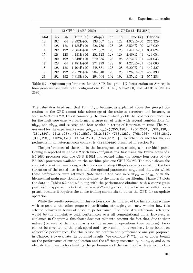
6.4. Experimental results

12 CPUs (1×E5-2680) 24 CPUs (2×E5-2680)

Mat. nb ib Time (s.) Gflop/s nb ib Time (s.) Gflop/s12 192 64 8.892E+00 138.667 128 128 4.922E+00 275.32913 128 128 1.188E+01 226.780 128 128 8.525E+00 316.02914 192 192 2.364E+01 221.062 128 128 1.444E+01 351.82415 128 128 4.151E+01 252.123 128 128 2.468E+01 424.05416 192 192 5.849E+01 272.335 128 128 3.734E+01 421.03317 128 64 7.181E+01 271.779 128 64 4.270E+01 457.06018 128 128 1.104E+02 248.881 128 128 6.209E+01 442.52719 192 192 2.212E+02 284.040 128 128 1.269E+02 489.39021 192 192 6.318E+02 294.604 192 192 3.352E+02 555.283

Table 6.2: Optimum performance for the STF fine-grain 1D factorization on Sirocco inhomogeneous case with both configurations 12 CPUs (1×E5-2680) and 24 CPUs (2×E5-2680).

The value ib is fixed such that ib = nbcpu because, as explained above the gemqrt op-eration on the GPU cannot take advantage of the staircase structure and because, asseen in Section 4.2.2, this is commonly the choice which yields the best performance. Asfor the multicore case, we performed a large set of tests with several combinations fornbcpu and nbgpu and selected the best results in terms of factorization time. The val-ues used for the experiments were (nbgpu,nbcpu)={(256,128), (256,256), (384,128),

(384,384), (512,128), (512,256), (512,512) (768,128), (768,256), (768,384),

(896,128), (1024,128), (1024,256), (1024,512) }. The scheduler used for the ex-periments in an heterogeneous context is heteroprio presented in Section 6.2.

The performance of the code in the heterogeneous case using a hierarchical parti-tioning is reported in Table 6.2 with two configurations: first using the twelve cores of aE5-2680 processor plus one GPU K40M and second using the twenty-four cores of twoE5-2680 processors available on the machine plus one GPU K40M. The table shows theshortest execution time along with the corresponding Gflop/s rates obtained for the fac-torization of the tested matrices and the optimal parameters nbgpu and nbcpu for whichthese performance were attained. Note that in the case were nbgpu = nbcpu, then thehierarchical-grain partitioning is equivalent to the fine-grain partitioning. Figure 6.7 plotsthe data in Tables 6.2 and 6.3 along with the performance obtained with a coarse-grainpartitioning approach; note that matrices #22 and #23 cannot be factorized with this ap-proach because it requires the entire trailing submatrix to be on the GPU for an updateoperation.

While the results presented in this section show the interest of the hierarchical schemewith respect to the other proposed partitioning strategies, one may wonder how thisscheme behaves in terms of absolute performance. The most straightforward referencewould be the cumulative peak performance over all computational units. However, asexplained in Chapter 2, this choice does not take into account the fact that, due to theirnature (because of their granularity or the nature of operations they perform), taskscannot be executed at the peak speed and may result in an excessively loose bound onachievable performance. For this reason we perform the performance analysis proposedin Chapter 2 to evaluate the obtained results. We compute tarea(p) as an upper boundon the performance of our application and the efficiency measures eg, et, ep, ec and er toidentify the main factors limiting the performance of the execution with respect to this

107

6. STF-parallel multifronatal QR method on heterogeneous

architecture

12 CPUs (1×E5-2680) 24 CPUs (2×E5-2680)+ 1 GPU (1×K40M) + 1 GPU (1×K40M)

Mat. nbgpu nbcpu Time (s.) Gflop/s nbgpu nbcpu Time (s.) Gflop/s12 384 384 8.302E+00 214.172 384 384 6.960E+00 255.46813 384 384 1.014E+01 309.913 256 256 9.731E+00 304.15514 384 384 1.803E+01 311.883 256 256 1.404E+01 382.01415 768 256 2.051E+01 525.130 512 256 2.026E+01 531.60916 896 128 2.810E+01 559.479 896 128 2.866E+01 548.54717 192 192 8.700E+01 246.755 256 256 6.797E+01 329.90518 512 256 4.918E+01 560.600 768 256 4.882E+01 564.73319 768 256 1.039E+02 611.656 796 384 8.763E+01 741.39921 768 256 2.792E+02 671.463 1024 256 2.403E+02 780.160

Table 6.3: Optimum performance for the STF hierarchical-grain 1D factorization onSirocco in heterogeneous case with both configurations 12 CPUs (1×E5-2680) + 1 GPU(1×K40M) and 24 CPUs (2×E5-2680) + 1 GPU (1×K40M).

0

200

400

600

800

1000

12 13 14 15 16 17 18 19 21

GFlop/s

Matrix #

Performance -- Sirocco

1 GPU -- coarse 12 CPUs -- fine 12 CPUs + 1 GPU -- hierarchical 24 CPUs -- fine 24 CPUs + 1 GPU -- hierarchical

Figure 6.7: Performance with heterogeneous vs multicore algorithms on Sirocco platform.

upper bound. Technically, tarea(p) and tarea(p) are computed by running two instances ofthe code, respectively, one with coarse grain partitioning and the other with hierarchicalpartitioning and solving, in both cases, the Linear Program 1 defined in Chapter 2. Notethat in order to generate the linear problem, it is necessary to run the code multiple timesso that StarPU can build accurate performance profiles.

Figure 6.8 shows the efficiency analysis for our code on the test matrices. With aruntime efficiency er greater than 0.9 for the tested matrices we see that the cost of theruntime system is negligible compared to the workload. In addition, the runtime overheadbecomes relatively smaller and smaller as the size of the problems increases. These results

108

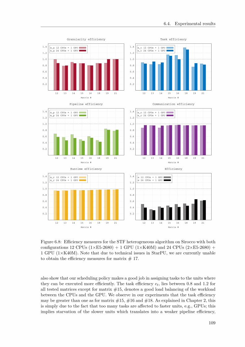
6.4. Experimental results

0.2

0.4

0.6

0.8

1.0

1.2

1.4

12 13 14 15 16 18 19 21

Matrix #

Granularity efficiency

e_g 12 CPUs + 1 GPUe_g 24 CPUs + 1 GPU

0.2

0.4

0.6

0.8

1.0

1.2

1.4

12 13 14 15 16 18 19 21

Matrix #

Task efficiency

e_t 12 CPUs + 1 GPUe_t 24 CPUs + 1 GPU

0.2

0.4

0.6

0.8

1.0

1.2

1.4

12 13 14 15 16 18 19 21

Matrix #

Pipeline efficiency

e_p 12 CPUs + 1 GPUe_p 24 CPUs + 1 GPU

0.2

0.4

0.6

0.8

1.0

1.2

1.4

12 13 14 15 16 18 19 21

Matrix #

Communication efficiency

e_c 12 CPUs + 1 GPUe_c 24 CPUs + 1 GPU

0.2

0.4

0.6

0.8

1.0

1.2

1.4

12 13 14 15 16 18 19 21

Matrix #

Runtime efficiency

e_r 12 CPUs + 1 GPUe_r 24 CPUs + 1 GPU

0.2

0.4

0.6

0.8

1.0

1.2

1.4

12 13 14 15 16 18 19 21

Matrix #

Efficiency

e 12 CPUs + 1 GPUe 24 CPUs + 1 GPU

Figure 6.8: Efficiency measures for the STF heterogeneous algorithm on Sirocco with bothconfigurations 12 CPUs (1×E5-2680) + 1 GPU (1×K40M) and 24 CPUs (2×E5-2680) +1 GPU (1×K40M). Note that due to technical issues in StarPU, we are currently unableto obtain the efficiency measures for matrix # 17.

also show that our scheduling policy makes a good job in assigning tasks to the units wherethey can be executed more efficiently. The task efficiency et, lies between 0.8 and 1.2 forall tested matrices except for matrix #15, denotes a good load balancing of the workloadbetween the CPUs and the GPU. We observe in our experiments that the task efficiencymay be greater than one as for matrix #15, #16 and #18. As explained in Chapter 2, thisis simply due to the fact that too many tasks are affected to faster units, e.g., GPUs; thisimplies starvation of the slower units which translates into a weaker pipeline efficiency,

109

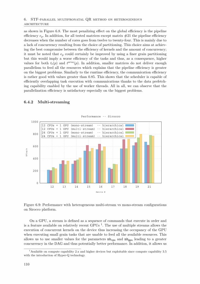
6. STF-parallel multifronatal QR method on heterogeneous

architecture

as shown in Figure 6.8. The most penalizing effect on the global efficiency is the pipelineefficiency ep. In addition, for all tested matrices except matrix #21 the pipeline efficiencydecreases when the number of cores goes from twelve to twenty-four. This is mainly due toa lack of concurrency resulting from the choice of partitioning. This choice aims at achiev-ing the best compromise between the efficiency of kernels and the amount of concurrency;it must be noted that ep could certainly be improved by using a finer grain partitioningbut this would imply a worse efficiency of the tasks and thus, as a consequence, highervalues for both tt(p) and tarea(p). In addition, smaller matrices do not deliver enoughparallelism to feed all the resources which explains that the pipeline efficiency is greateron the biggest problems. Similarly to the runtime efficiency, the communication efficiencyis rather good with values greater than 0.85. This shows that the scheduler is capable ofefficiently overlapping task execution with communications thanks to the data prefetch-ing capability enabled by the use of worker threads. All in all, we can observe that theparallelization efficiency is satisfactory especially on the biggest problems.

6.4.2 Multi-streaming

0

200

400

600

800

1000

12 13 14 15 16 17 18 19 21

GFlop/s

Matrix #

Performance -- Sirocco

12 CPUs + 1 GPU (mono-stream) -- hierarchical 12 CPUs + 1 GPU (multi-stream) -- hierarchical24 CPUs + 1 GPU (mono-stream) -- hierarchical 24 CPUs + 1 GPU (multi-stream) -- hierarchical

Figure 6.9: Performance with heterogeneous multi-stream vs mono-stream configurationson Sirocco platform.

On a GPU, a stream is defined as a sequence of commands that execute in order andis a feature available on relatively recent GPUs 1. The use of multiple streams allows theexecution of concurrent kernels on the device thus increasing the occupancy of the GPUwhen executing small grain tasks that are unable to feed all the available resources. Thisallows us to use smaller values for the parameters nbcpu and nbgpu leading to a greaterconcurrency in the DAG and thus potentially better performance. In addition, it allows us

1Available on compute capability 2.x and higher devices but exploitable since compute capability 3.5with the introduction of Hyper-Q technology.

110

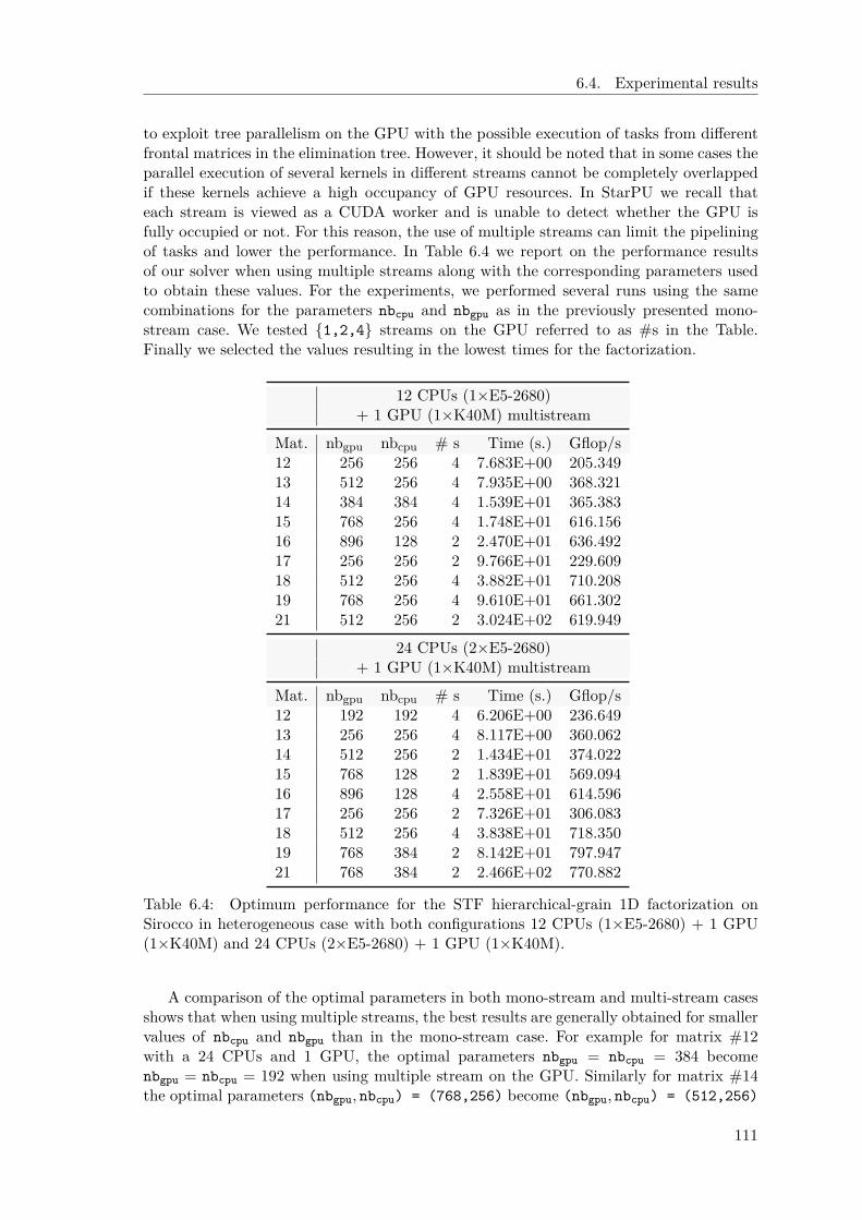
6.4. Experimental results

to exploit tree parallelism on the GPU with the possible execution of tasks from differentfrontal matrices in the elimination tree. However, it should be noted that in some cases theparallel execution of several kernels in different streams cannot be completely overlappedif these kernels achieve a high occupancy of GPU resources. In StarPU we recall thateach stream is viewed as a CUDA worker and is unable to detect whether the GPU isfully occupied or not. For this reason, the use of multiple streams can limit the pipeliningof tasks and lower the performance. In Table 6.4 we report on the performance resultsof our solver when using multiple streams along with the corresponding parameters usedto obtain these values. For the experiments, we performed several runs using the samecombinations for the parameters nbcpu and nbgpu as in the previously presented mono-stream case. We tested {1,2,4} streams on the GPU referred to as #s in the Table.Finally we selected the values resulting in the lowest times for the factorization.

12 CPUs (1×E5-2680)+ 1 GPU (1×K40M) multistream

Mat. nbgpu nbcpu # s Time (s.) Gflop/s12 256 256 4 7.683E+00 205.34913 512 256 4 7.935E+00 368.32114 384 384 4 1.539E+01 365.38315 768 256 4 1.748E+01 616.15616 896 128 2 2.470E+01 636.49217 256 256 2 9.766E+01 229.60918 512 256 4 3.882E+01 710.20819 768 256 4 9.610E+01 661.30221 512 256 2 3.024E+02 619.949

24 CPUs (2×E5-2680)+ 1 GPU (1×K40M) multistream

Mat. nbgpu nbcpu # s Time (s.) Gflop/s12 192 192 4 6.206E+00 236.64913 256 256 4 8.117E+00 360.06214 512 256 2 1.434E+01 374.02215 768 128 2 1.839E+01 569.09416 896 128 4 2.558E+01 614.59617 256 256 2 7.326E+01 306.08318 512 256 4 3.838E+01 718.35019 768 384 2 8.142E+01 797.94721 768 384 2 2.466E+02 770.882

Table 6.4: Optimum performance for the STF hierarchical-grain 1D factorization onSirocco in heterogeneous case with both configurations 12 CPUs (1×E5-2680) + 1 GPU(1×K40M) and 24 CPUs (2×E5-2680) + 1 GPU (1×K40M).

A comparison of the optimal parameters in both mono-stream and multi-stream casesshows that when using multiple streams, the best results are generally obtained for smallervalues of nbcpu and nbgpu than in the mono-stream case. For example for matrix #12with a 24 CPUs and 1 GPU, the optimal parameters nbgpu = nbcpu = 384 becomenbgpu = nbcpu = 192 when using multiple stream on the GPU. Similarly for matrix #14the optimal parameters (nbgpu, nbcpu) = (768,256) become (nbgpu, nbcpu) = (512,256)

111

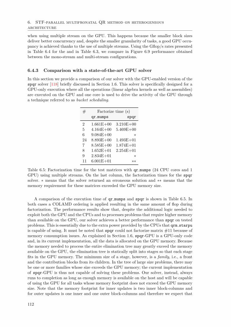
6. STF-parallel multifronatal QR method on heterogeneous

architecture

when using multiple stream on the GPU. This happens because the smaller block sizesdeliver better concurrency and, despite the smaller granularity of tasks, a good GPU occu-pancy is achieved thanks to the use of multiple streams. Using the Gflop/s rates presentedin Table 6.4 for the and in Table 6.3, we compare in Figure 6.9 performance obtainedbetween the mono-stream and multi-stream configurations.

6.4.3 Comparison with a state-of-the-art GPU solver

In this section we provide a comparison of our solver with the GPU-enabled version of thespqr solver [118] briefly discussed in Section 1.6. This solver is specifically designed for aGPU-only execution where all the operations (linear algebra kernels as well as assemblies)are executed on the GPU and one core is used to drive the activity of the GPU througha technique referred to as bucket scheduling.

# Factorize time (s)qr mumps spqr

2 1.661E+00 3.210E+005 4.164E+00 5.469E+006 9.084E+00 ∗24 8.893E+00 1.493E+017 8.585E+00 1.874E+018 1.652E+01 2.254E+019 2.834E+01 ∗11 6.001E+01 ∗∗

Table 6.5: Factorization time for the test matrices with qr mumps (24 CPU cores and 1GPU) using multiple streams. On the last column, the factorization times for the spqr

solver. ∗ means that the solver returned an erroneous solution and ∗∗ means that thememory requirement for these matrices exceeded the GPU memory size.

A comparison of the execution time of qr mumps and spqr is shown in Table 6.5. Inboth cases a COLAMD ordering is applied resulting in the same amount of flop duringfactorization. The performance results show that, despite the additional logic needed toexploit both the GPU and the CPUs and to processes problems that require higher memorythan available on the GPU, our solver achieves a better performance than spqr on testedproblems. This is essentially due to the extra power provided by the CPUs that qrm starpu

is capable of using. It must be noted that spqr could not factorize matrix #11 because ofmemory consumption issues. As explained in Section 1.6, spqr-GPU is a GPU-only codeand, in its current implementation, all the data is allocated on the GPU memory. Becausethe memory needed to process the entire elimination tree may greatly exceed the memoryavailable on the GPU, the elimination tree is statically split into stages so that each stagefits in the GPU memory. The minimum size of a stage, however, is a family, i.e., a frontand the contribution blocks from its children. In the tree of large size problems, there maybe one or more families whose size exceeds the GPU memory; the current implementationof spqr-GPU is thus not capable of solving these problems. Our solver, instead, alwaysruns to completion as long as enough memory is available on the host and will be capableof using the GPU for all tasks whose memory footprint does not exceed the GPU memorysize. Note that the memory footprint for inner updates is two inner block-columns andfor outer updates is one inner and one outer block-columns and therefore we expect that

112

6.5. Possible minor, technical improvements

most of the tasks will fit in the GPU memory unless the size of the frontal matrices isextremely high.

In two cases (matrices #6 and #9) the spqr solver returned an erroneous solution.

6.5 Possible minor, technical improvements

The code we implemented and that was used to produce the experimental results pre-sented above was principally developed with the objective of validating and assessing theeffectiveness of the front partitioning and tasks scheduling methods discussed in the previ-ous sections. There are, nonetheless, a number of minor technical improvements that canbe applied to the code and that are likely to bring substantial benefits to its performanceand scalability. Although we plan to pursue these developments in future work, we brieflydiscuss them in this section.

• GPU memory allocation. In our current implementation, frontal matrices arealways allocated on the host memory, which implies that the data has to be trans-ferred to the GPU before being processed by GPU tasks. In some specific cases itshould be possible to allocate the memory directly on the device which allows forsaving communications. This is, for example, the case when do subtree tasks areexecuted on the GPU.

• Memory pinning. Memory pinning enables faster data transfers between the hostand the device. Although pinned memory allocations have a higher latency, this isproven to be extremely beneficial for the factorization of a large dense matrix. How-ever, in the case of our code, which uses block storage, many, small size allocationsare executed for each frontal matrix, which renders the pinning overhead unbearable.Moreover, because all the allocations are done by the master thread, this overheadslows down the submission of tasks. It should be possible to perform pinned alloca-tions selectively only on those fronts which are more likely to be processed on theGPU, or to defer the allocation to the init task in order to prevent the overheadfrom slowing down the submission of tasks.

• Staircase-aware GPU kernels. As explained in Section 6.3, qrm starpu currentlyrelies on MAGMA routines for performing inner and outer updates. As a result, weare not fully capable of taking advantage of the fronts staircase structure. Imple-menting kernels that can exploit the staircase would readily result in a performanceimprovement.

• GPU panel factorization and assemblies. At the moment we do not have a GPUimplementation for the geqrt and assembly tasks. Although these operations arelikely to have small acceleration factors relative to the updates, they can still be runfaster on the GPU and, moreover, being capable of computing them on the devicewould allow us to save some data transfers.

• Efficient subtrees. The performance of GPU do subtree tasks can be improvedby employing approaches like the one used for spqr-GPU or SSIDS (see Section 1.6).

113

Chapter 7

Associated work

7.1 PTG multifrontal QR method

In the previous chapters we presented the parallelization of a multifrontal method basedon an STF model and implemented with the StarPU runtime system. In this section wepropose an alternative approach using a PTG model presented in Section 1.4.1. This par-allel version of the multifrontal method is implemented with the PaRSEC runtime systemintroduced in Section 1.4 and referred to as qrm parsec. As explained in Section 1.4.1,contrary to the STF model where task dependencies are inferred by the runtime system,the PTG model requires the explicit declaration of all the dependencies in the DAG to theruntime system. In the PaRSEC runtime system, this is done through a specific languagecalled JDF. This property allows great flexibility in the expression of dependencies andprevents the occurrence of unnecessary dependencies in the computed DAG as is the casefor the assembly tasks in the implementation described in Chapters 3, 4, 5 and 6. On theother hand, the expression of the DAG for the multifrontal QR factorization represents achallenge due to the complexity of its dependency pattern and because it is only knowndynamically at runtime.

A simple approach for the implementation of the PTG-parallel factorization consists inexpressing the whole DAG in a single JDF. This solution however raises several problems.First the dependency pattern associated with the factorization of the frontal matricesand the assembly operations is dynamically known during the tree traversal and PaRSECdoes not currently support this property. This approach is therefore not suited and as aconsequence prevents us from using inter-level parallelism as we show below. It should benoted that this is only a technical limitation of the runtime system and not of the pro-gramming model. Regarding the PTG model, it is conceivable to represent a DAG whichis dynamically built as it is unrolled during execution. The second reason for choosinganother approach is that the complexity of the dependency pattern increases with theamount of tasks in the DAG. In the proposed implementation of qrm parsec we use asimpler approach based on hierarchical DAGs. We consider a two-level hierarchy with anouter DAG and multiple inner DAGs spawned by the tasks of the higher level DAG: theouter DAG contains tasks related to the activation, deactivation, initialization and assem-bly of the nodes of the elimination tree whereas each inner DAG contains all the tasksfor factorizing the related front. This approach is illustrated in Figure 7.1 where threedifferent DAGs denoted by 1, 2 and 3 are spawned by tasks in the outer DAG. Note thatthis approach is equivalent to the one used in the UHM solvers presented in Section 1.6.

The PaRSEC implementation of the multifrontal QR factorization in our solver is splitinto several JDF files:

115

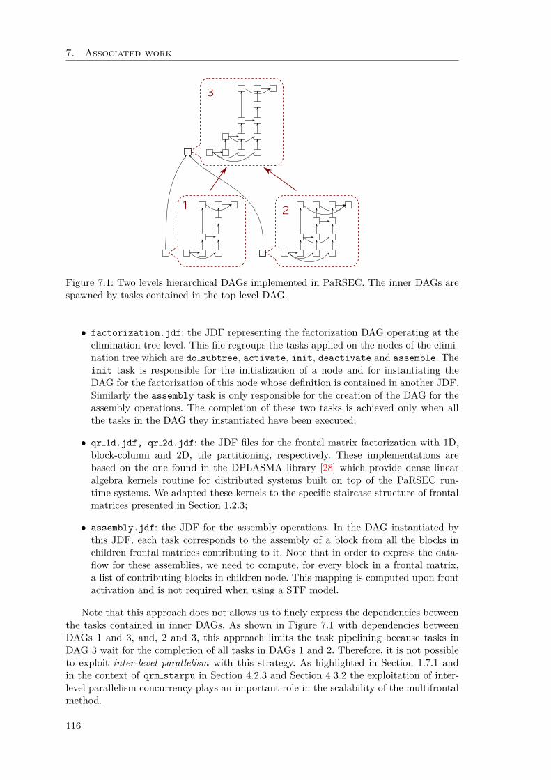
7. Associated work

12

3

Figure 7.1: Two levels hierarchical DAGs implemented in PaRSEC. The inner DAGs arespawned by tasks contained in the top level DAG.

• factorization.jdf: the JDF representing the factorization DAG operating at theelimination tree level. This file regroups the tasks applied on the nodes of the elimi-nation tree which are do subtree, activate, init, deactivate and assemble. Theinit task is responsible for the initialization of a node and for instantiating theDAG for the factorization of this node whose definition is contained in another JDF.Similarly the assembly task is only responsible for the creation of the DAG for theassembly operations. The completion of these two tasks is achieved only when allthe tasks in the DAG they instantiated have been executed;

• qr 1d.jdf, qr 2d.jdf: the JDF files for the frontal matrix factorization with 1D,block-column and 2D, tile partitioning, respectively. These implementations arebased on the one found in the DPLASMA library [28] which provide dense linearalgebra kernels routine for distributed systems built on top of the PaRSEC run-time systems. We adapted these kernels to the specific staircase structure of frontalmatrices presented in Section 1.2.3;

• assembly.jdf: the JDF for the assembly operations. In the DAG instantiated bythis JDF, each task corresponds to the assembly of a block from all the blocks inchildren frontal matrices contributing to it. Note that in order to express the data-flow for these assemblies, we need to compute, for every block in a frontal matrix,a list of contributing blocks in children node. This mapping is computed upon frontactivation and is not required when using a STF model.

Note that this approach does not allows us to finely express the dependencies betweenthe tasks contained in inner DAGs. As shown in Figure 7.1 with dependencies betweenDAGs 1 and 3, and, 2 and 3, this approach limits the task pipelining because tasks inDAG 3 wait for the completion of all tasks in DAGs 1 and 2. Therefore, it is not possibleto exploit inter-level parallelism with this strategy. As highlighted in Section 1.7.1 andin the context of qrm starpu in Section 4.2.3 and Section 4.3.2 the exploitation of inter-level parallelism concurrency plays an important role in the scalability of the multifrontalmethod.

116

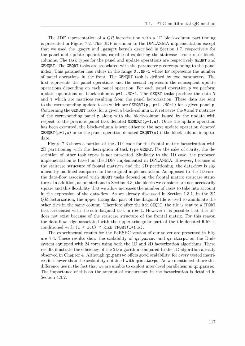
7.1. PTG multifrontal QR method

The JDF representation of a QR factorization with a 1D block-column partitioningis presented in Figure 7.2. This JDF is similar to the DPLASMA implementation exceptthat we used the geqrt and gemqrt kernels described in Section 1.7, respectively forthe panel and update operations, capable of exploiting the staircase structure of block-columns. The task types for the panel and update operations are respectively GEQRT andGEMQRT. The GEQRT tasks are associated with the parameter p corresponding to the panelindex. This parameter has values in the range 0..NP-1 where NP represents the numberof panel operations in the front. The GEMQRT task is defined by two parameters. Thefirst represents the panel operations and the second represents the subsequent updateoperations depending on each panel operation. For each panel operation p we performupdate operations on block-columns p+1..NC-1. The GEQRT tasks produce the data V

and T which are matrices resulting from the panel factorization. These data are sentto the corresponding update tasks which are GEMQRT(p, p+1..NC-1) for a given panel p.Concerning the GEMQRT tasks, for a given a block-column u, it retrieves the V and T matricesof the corresponding panel p along with the block-column issued by the update withrespect to the previous panel task denoted GEMQRT(p-1,u). Once the update operationhas been executed, the block-column is sent either to the next update operation denotedGEMQRT(p+1,u) or to the panel operation denoted GEQRT(u) if the block-column is up-to-date.

Figure 7.3 shows a portion of the JDF code for the frontal matrix factorization with2D partitioning with the description of task type GEQRT. For the sake of clarity, the de-scription of other task types is not presented. Similarly to the 1D case, the proposedimplementation is based on the JDFs implemented in DPLASMA. However, because ofthe staircase structure of frontal matrices and the 2D partitioning, the data-flow is sig-nificantly modified compared to the original implementation. As opposed to the 1D case,the data-flow associated with GEQRT tasks depend on the frontal matrix staircase struc-tures. In addition, as pointed out in Section 4.3, the blocks we consider are not necessarilysquare and this flexibility that we allow increases the number of cases to take into accountin the expression of the data-flow. As we already discussed in Section 1.3.1, in the 2DQR factorization, the upper triangular part of the diagonal tile is used to annihilate theother tiles in the same column. Therefore after the kth GEQRT, the tile is sent to a TPQRT

task associated with the sub-diagonal task in row i. However it is possible that this tiledoes not exist because of the staircase structure of the frontal matrix. For this reasonthe data-flow edge associated with the upper triangular part of the tile denoted R kk isconditioned with (i < lct) ? R kk TPQRT(i+1,k).

The experimental results for the PaRSEC version of our solver are presented in Fig-ure 7.4. These results show the scalability of qr parsec and qr starpu on the Dudesystem equipped with 24 cores using both the 1D and 2D factorization algorithms. Theseresults illustrate the efficiency of the 2D algorithm compared to the 1D algorithm alreadyobserved in Chapter 4. Although qr parsec offers good scalability, for every tested matri-ces it is lower than the scalability obtained with qrm starpu. As we mentioned above thisdifference lies in the fact that we are unable to exploit inter-level parallelism in qr parsec.The importance of this on the amount of concurrency in the factorization is detailed inSection 4.3.2.

117

7. Associated work

1 GEQRT (p)

3 p = 0 .. (NP -1)

5 : A(0,p)

7 RW A_p <- (p==0) ? A(0,p) : C_u GEMQRT (p-1, p)-> (p < NC -1) ? V_p GEMQRT (p, (p+1) ..(NC -1))

9 -> A(0,p)

11 RW T_p <- T(0, p) [type = LITTLE_T ]-> (p < NC -1) ? T_p GEMQRT (p, (p+1) ..(NC -1)) [type = LITTLE_T ]

13 -> T(0,p)

15 ;NC

17 BODY{

19

_geqrt_stair (&m, &n, &ib ,21 & stair [off], &off ,

A_p + off , &lda ,23 T_p , &ldt ,

work , &info);25

}27 END

29 GEMQRT (p, u)

31 p = 0..(NP -1)u = (p+1) ..(NC -1)

33

: A(0,u)35

READ V_p <- A_p GEQRT (p)37 READ T_p <- T_p GEQRT (p) [type = LITTLE_T ]

RW C_u <- (p==0) ? A(0,u) : C_u GEMQRT (p-1, u)39 -> ((u == p+1) && (u <= (NP -1))) ? A_p GEQRT (u)

-> ((u > p+1) && (p < (NP -1))) ? C_u GEMQRT (p+1, u)41

; (NC -u)43

BODY45 {

47 _gemqrt_stair ("l", "t",&m, &j, &k, &ib ,

49 & stair [off], &off ,V_p + off , &ldv ,

51 T_p , &ldt ,C_u + off , &ldc ,

53 work , &info);

55 }

57 END

Figure 7.2: Code for the 1D block-column dense QR factorization with PaRSEC.

118

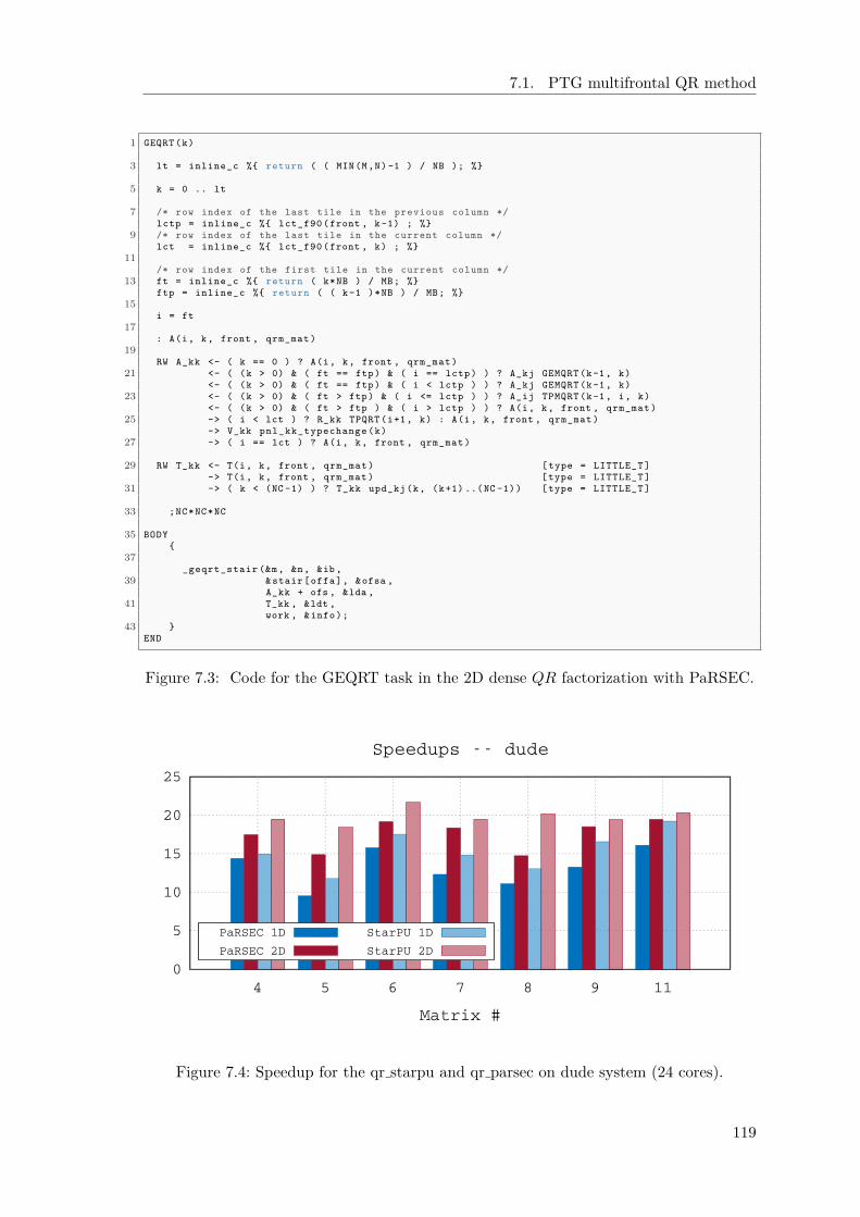
7.1. PTG multifrontal QR method

1 GEQRT (k)

3 lt = inline_c %{ return ( ( MIN(M,N) -1 ) / NB ); %}

5 k = 0 .. lt

7 /* row index of the last tile in the previous column */lctp = inline_c %{ lct_f90 (front , k -1) ; %}

9 /* row index of the last tile in the current column */lct = inline_c %{ lct_f90 (front , k) ; %}

11

/* row index of the first tile in the current column */13 ft = inline_c %{ return ( k*NB ) / MB; %}

ftp = inline_c %{ return ( ( k -1 )*NB ) / MB; %}15

i = ft17

: A(i, k, front , qrm_mat )19

RW A_kk <- ( k == 0 ) ? A(i, k, front , qrm_mat )21 <- ( (k > 0) & ( ft == ftp) & ( i == lctp) ) ? A_kj GEMQRT (k-1, k)

<- ( (k > 0) & ( ft == ftp) & ( i < lctp ) ) ? A_kj GEMQRT (k-1, k)23 <- ( (k > 0) & ( ft > ftp) & ( i <= lctp ) ) ? A_ij TPMQRT (k-1, i, k)

<- ( (k > 0) & ( ft > ftp ) & ( i > lctp ) ) ? A(i, k, front , qrm_mat )25 -> ( i < lct ) ? R_kk TPQRT (i+1, k) : A(i, k, front , qrm_mat )

-> V_kk pnl_kk_typechange (k)27 -> ( i == lct ) ? A(i, k, front , qrm_mat )

29 RW T_kk <- T(i, k, front , qrm_mat ) [type = LITTLE_T ]-> T(i, k, front , qrm_mat ) [type = LITTLE_T ]

31 -> ( k < (NC -1) ) ? T_kk upd_kj (k, (k+1) ..(NC -1)) [type = LITTLE_T ]

33 ;NC*NC*NC

35 BODY{

37

_geqrt_stair (&m, &n, &ib ,39 & stair [offa], &ofsa ,

A_kk + ofs , &lda ,41 T_kk , &ldt ,

work , &info);43 }

END

Figure 7.3: Code for the GEQRT task in the 2D dense QR factorization with PaRSEC.

0

5

10

15

20

25

4 5 6 7 8 9 11

Matrix #

Speedups -- dude

PaRSEC 1D

PaRSEC 2D

StarPU 1D

StarPU 2D

Figure 7.4: Speedup for the qr starpu and qr parsec on dude system (24 cores).

119

7. Associated work

7.2 Simulation of qrm starpu with StarPU SimGrid

The development of scientific software that aims to be portable across different archi-tectures requires a considerable amount of performance analysis and tuning. This is avery challenging task to achieve for large and complex codes which feature an irregularworkload and which are designed for modern computing platforms equipped with het-erogeneous processing units. This is even more difficult if one considers that access tocomputing platforms with the desired characteristics may be limited if at all possible. Inthe case of runtime-based software, this issue can be addressed by taking advantage ofthe fact that the runtime has full control over the execution of the tasks in which theworkload is decomposed: the runtime system can be instructed not to actually executethe tasks, but instead to simulate their execution reproducing their resource consumption(be it PU time or memory) on the target architecture. Because the tasks are not actuallyexecuted, and therefore the resources are not actually consumed, this technique allows thesimulation of the execution of very large workloads on large and complex architectureseven on systems with a relatively limited amount of resources like a laptop computer.

Researchers from the MESCAL project at the LIG Laboratory of Grenoble have re-alized a coarse-grain hybrid simulation/emulation of StarPU applications [107] on top ofSimGrid[36], a simulation toolkit specifically designed for distributed system simulation.In this approach the application (i.e., the work of the master thread) and runtime areemulated as their actual code is executed and the tasks submission and scheduling aretherefore done as in a real execution; tasks, however, are not actually executed but simu-lated. An initial calibration of the target machine is run first to derive performance profilesand models (interconnect topology, data transfers, computation kernels) that are given asinput to SimGrid. Subsequent simulations can then be performed in a reproducible way onpersonal commodity laptops without requiring any further access to the target machines.

This approach was proved capable of achieving accurate performance prediction oftwo dense linear algebra algorithms on a number of heterogeneous systems [108], yetits effectiveness on more irregular and heterogeneous workloads had to be assessed. Forthis purpose, we collaborated [0] with the authors of the StarPU-SimGrid platform toevaluate the accuracy of this simulation engine on the qrm starpu solver, precisely onthe 1D STF variant presented in Section 4.2. Compared to the abovementioned study onthe simulation of dense linear algebra applications with StarPU and SimGrid, the maindifficulty arises from the application structure and from the larger variety of computationtasks or kernels called with a wide variety of input parameters. When working with densematrices, it is common to use a global fixed block size and a given kernel type (e.g.,gemm) is therefore always called with the same parameters throughout the execution,which makes its duration on the same processing unit very stable and easy to model. Inthe qrm starpu factorization, the amount of work that has to be done by a given kernelgreatly depends on its input parameters. These parameters may or may not be explicitlygiven to the StarPU runtime and we thus had to rework the qrm starpu task submissionmodel to ensure StarPU can propagate this information to SimGrid. The modelling of thedifferent kernels used in qrm starpu was done using the following assumptions:

• geqrt: this kernel is a simple wrapper around the corresponding LAPACK routineand thus it can be completely characterized by the size m×n of the block it operateson. This information is readily available to StarPU through the task parameters nb

(the column width), mb (the block-column height) and bk (the front factorizationstage or panel number). Given that m = mb − (bk − 1) × nb and n = nb, the

120

7.2. Simulation of qrm starpu with StarPU SimGrid

complexity of this kernel is

Tgeqrt = a + 2b(nb2 × mb) − 2c(nb3 × bk) +4d

3nb3,

where a, b, c and d are machine and memory hierarchy dependent constant coeffi-cients.

• gemqrt: The duration of the gemqrt kernel also depends on the geometry of thedata it operates upon, defined by the same mb, nb, and bk parameters. This kernelssimply wraps the LAPACK gemqrt routine which applies k Householder reflectionsof size m, m − 1, ..., m − k+1 on a matrix of size m × n where m, n and k are equalto mb − (bk − 1) × nb, nb and nb, respectively. Therefore, its a priori complexity isdefined as:

Tgemqrt = a′ + 4b′(nb2 × mb) − 4c′(nb3 × bk) + 3d′nb3

• init: the execution time of this kernel depends on the number of coefficients in thefronts (because they have to be initialized to zero) #Zeros and the number #Aasmof coefficients from the input sparse matrix that have to be assembled in the front.These parameters had to be added to the signature of the task submission routinein order to make their value available to StarPU.

• assemble: the execution time of tihs kernel solely depends on the number #Casm ofcoefficients from the block-column that have to be assembled into the parent front.This parameter had to be added to the signature of the task submission routine inorder to make its value available to StarPU.

• do subtree: the execution time of this kernel mostly depends on the number of flopsperformed therein and on the number of fronts in the subtree (this gives a measureof the granularity of operations and thus their efficiency). These parameters had tobe added to the signature of the task submission routine in order to make their valueavailable to StarPU. Note that this data is computed during the analysis phase andthus already available.

• deactivate: this kernel is considered negligible as it only acounts for less than 1%of the total execution time.

To evaluate the quality of our approach, we used two different kinds of nodes fromthe Plafrim1 platform. The fourmi nodes feature 2 Quad-core Nehalem Intel Xeon X5550with a frequency of 2.66 GHz and 24 GB of RAM memory and the riri nodes comprise 4Deca-core Intel Xeon E7-4870 with a frequency of 2.40 GHz and 1 TB of RAM memory.The fourmi nodes proved to be easier to model as their CPU architecture is well balancedwith 4 cores sharing L3 cache on each of the 2 NUMA nodes. Such a configuration leadsto little cache contention. However, the RAM of these nodes is limited and thereby limitsthe matrices that can be factorized to a certain size. Although the huge memory of theriri machine puts almost no restriction on the matrix choice, its memory hierarchy with10 cores sharing the same L3 cache lead to cache contention that can be tricky to model.

The execution time of a single kernel on a certain machine greatly depends on the ma-chine characteristics (namely CPU frequency, memory hierarchy, compiler optimization,etc.). Obtaining accurate timing is thus a critical step of the modelling. To predict the

1https://plafrim.bordeaux.inria.fr/

121

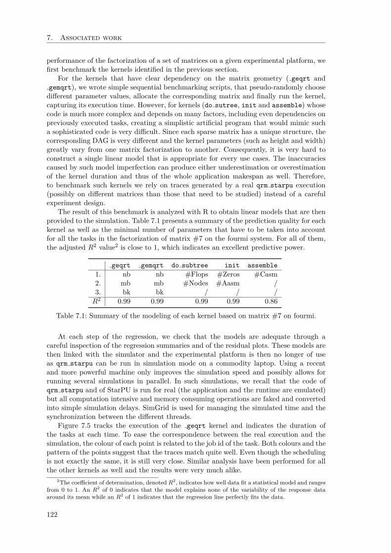
7. Associated work

performance of the factorization of a set of matrices on a given experimental platform, wefirst benchmark the kernels identified in the previous section.

For the kernels that have clear dependency on the matrix geometry ( geqrt andgemqrt), we wrote simple sequential benchmarking scripts, that pseudo-randomly choosedifferent parameter values, allocate the corresponding matrix and finally run the kernel,capturing its execution time. However, for kernels (do sutree, init and assemble) whosecode is much more complex and depends on many factors, including even dependencies onpreviously executed tasks, creating a simplistic artificial program that would mimic sucha sophisticated code is very difficult. Since each sparse matrix has a unique structure, thecorresponding DAG is very different and the kernel parameters (such as height and width)greatly vary from one matrix factorization to another. Consequently, it is very hard toconstruct a single linear model that is appropriate for every use cases. The inaccuraciescaused by such model imperfection can produce either underestimation or overestimationof the kernel duration and thus of the whole application makespan as well. Therefore,to benchmark such kernels we rely on traces generated by a real qrm starpu execution(possibly on different matrices than those that need to be studied) instead of a carefulexperiment design.

The result of this benchmark is analyzed with R to obtain linear models that are thenprovided to the simulation. Table 7.1 presents a summary of the prediction quality for eachkernel as well as the minimal number of parameters that have to be taken into accountfor all the tasks in the factorization of matrix #7 on the fourmi system. For all of them,the adjusted R2 value2 is close to 1, which indicates an excellent predictive power.

geqrt gemqrt do subtree init assemble

1. nb nb #Flops #Zeros #Casm2. mb mb #Nodes #Aasm /3. bk bk / / /

R2 0.99 0.99 0.99 0.99 0.86

Table 7.1: Summary of the modeling of each kernel based on matrix #7 on fourmi.

At each step of the regression, we check that the models are adequate through acareful inspection of the regression summaries and of the residual plots. These models arethen linked with the simulator and the experimental platform is then no longer of useas qrm starpu can be run in simulation mode on a commodity laptop. Using a recentand more powerful machine only improves the simulation speed and possibly allows forrunning several simulations in parallel. In such simulations, we recall that the code ofqrm starpu and of StarPU is run for real (the application and the runtime are emulated)but all computation intensive and memory consuming operations are faked and convertedinto simple simulation delays. SimGrid is used for managing the simulated time and thesynchronization between the different threads.

Figure 7.5 tracks the execution of the geqrt kernel and indicates the duration ofthe tasks at each time. To ease the correspondence between the real execution and thesimulation, the colour of each point is related to the job id of the task. Both colours and thepattern of the points suggest that the traces match quite well. Even though the schedulingis not exactly the same, it is still very close. Similar analysis have been performed for allthe other kernels as well and the results were very much alike.

2The coefficient of determination, denoted R2, indicates how well data fit a statistical model and ranges

from 0 to 1. An R2 of 0 indicates that the model explains none of the variability of the response data

around its mean while an R2 of 1 indicates that the regression line perfectly fits the data.

122

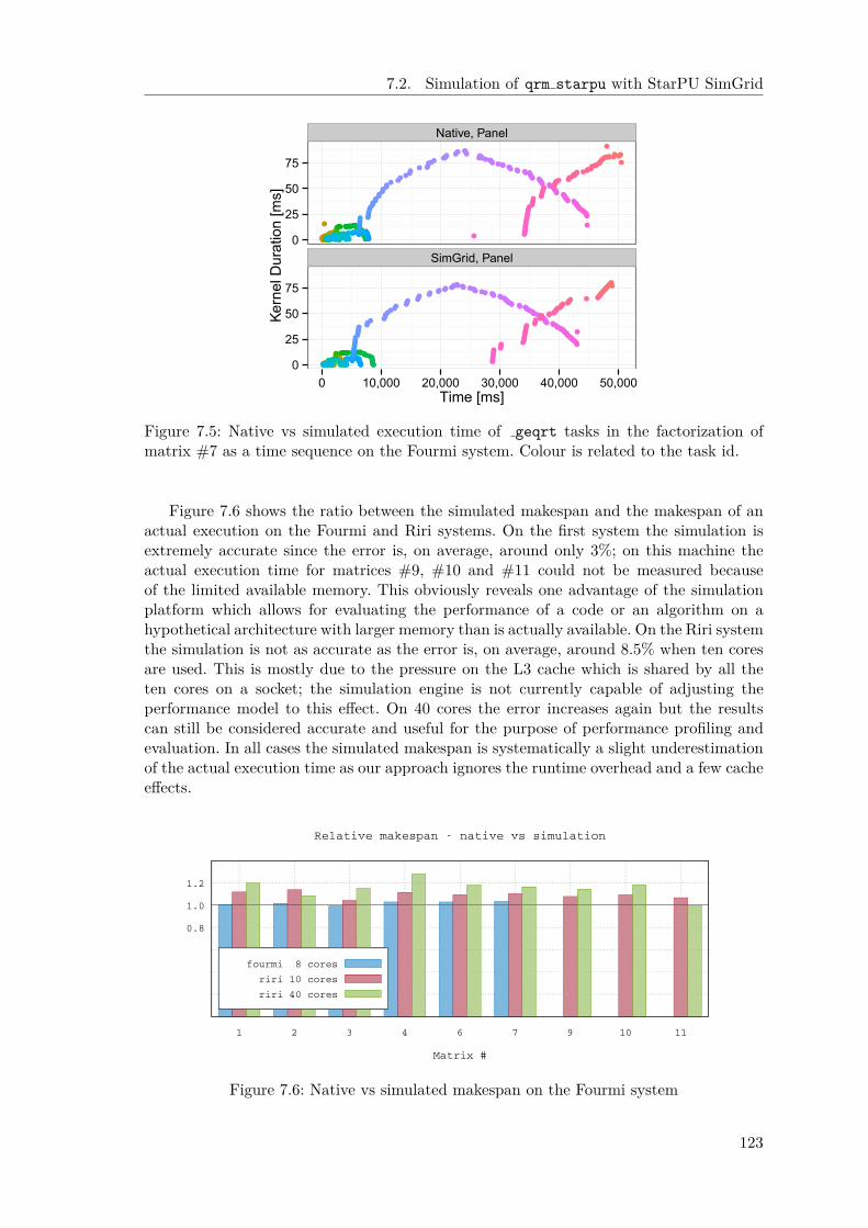
7.2. Simulation of qrm starpu with StarPU SimGrid

●●●●●●●●●●●●●●●●●●●●●●●●●●●●●●●●●●●●●●●●●●●●●●●●●●●●●●●●●●●●●●●●●●●●●●

●

●●●●●●●●●●●●●●●●●●●●●●●●●●●●●●●●●●●●●●●●●●●●●●●●●●●●●●●●●●●●●●●●●●●●●●●●●●●●●●●●●●●●●●●●●●●●●●●●●●●●●●●●●●●●●●●●●●●●●●●●●●●●●●●●●●●●●●●●●●●●●●●●●

●●●●●●●●●●●●●●●●●●●●●●●●●●● ●●●●●●●●●●●●●●●●●●●●●●●●●●●●●●●●●●●●●●●●●●●●●●●●●●●●●●●●

●●●●●●●●●●●●●●●●●●●●●●●●●● ●●

●●●●●●●●●●●●●●●●

●●●

● ●●●●●

●●●●●●●

●●●●●●●●●●●●●●●●●●●●●●●●●●●●●●●●●●●●●●●●●●●●●●●●●●●●●●●●●●●●●●●●●●●

●

● ●●●●●●●●●●●●●●●●●●● ●●

●●●● ●●●

●●●● ●●●

●●●●●●●●

●●●●●●●●●●●●

●

●●●●●●●●

●

●●●●●●●●●●●●●●●●●●●●●●●●●●●●●●●●●●●●●●●●●●●●●●●●●●●●●●●●●●●●●●●●●●●●●●●●●●●●●●●●●●●●●●●●●●●●●●●●●●●●●●●●●●●●●●●●●●●●●●●●●●●●●●●●●●●●●●●●●●●●●●●●●●●●●●●●●●●●●●●●●●●●●●●●●●●●●●●●●●●●●●●●●●●●●●●●●●●●●●●●●●●●●●●●●●●●●●●●

●●●●●●●●●●●●●●●●●●●●●●●●●●● ●●●●●●●●●●●●●●●●●●●●●●●●●●●●●●●●●●●●●●●●●●●●●●●●●●●●●●●●●●●●●●●●

●●●●●●●●●●●●●●●●●●●●●●●●●●● ●●

● ●●●●●●● ●●

● ●●● ●●

●●●●●●●●●●●●●●●●●●●●●●●●●●●●●● ●●●●●●●●●●●●●●●●●●●●●●●●●●●●●●●●●●●●●●●●●●●●

●

●●●●●●●●●●● ●●

●●●●●●●●

●●●●●●●●●●●

●●●●●●●●●●●●●● ● ●●●

●●●●●●●●●●●●●●●●

Native, Panel

SimGrid, Panel

0

25

50

75

0

25

50

75

0 10,000 20,000 30,000 40,000 50,000

Time [ms]

Ke

rne

l D

ura

tio

n [

ms]

Figure 7.5: Native vs simulated execution time of geqrt tasks in the factorization ofmatrix #7 as a time sequence on the Fourmi system. Colour is related to the task id.

Figure 7.6 shows the ratio between the simulated makespan and the makespan of anactual execution on the Fourmi and Riri systems. On the first system the simulation isextremely accurate since the error is, on average, around only 3%; on this machine theactual execution time for matrices #9, #10 and #11 could not be measured becauseof the limited available memory. This obviously reveals one advantage of the simulationplatform which allows for evaluating the performance of a code or an algorithm on ahypothetical architecture with larger memory than is actually available. On the Riri systemthe simulation is not as accurate as the error is, on average, around 8.5% when ten coresare used. This is mostly due to the pressure on the L3 cache which is shared by all theten cores on a socket; the simulation engine is not currently capable of adjusting theperformance model to this effect. On 40 cores the error increases again but the resultscan still be considered accurate and useful for the purpose of performance profiling andevaluation. In all cases the simulated makespan is systematically a slight underestimationof the actual execution time as our approach ignores the runtime overhead and a few cacheeffects.

0.8

1.0

1.2

1 2 3 4 6 7 9 10 11

Matrix #

Relative makespan - native vs simulation

fourmi 8 cores

riri 10 cores

riri 40 cores

Figure 7.6: Native vs simulated makespan on the Fourmi system

123

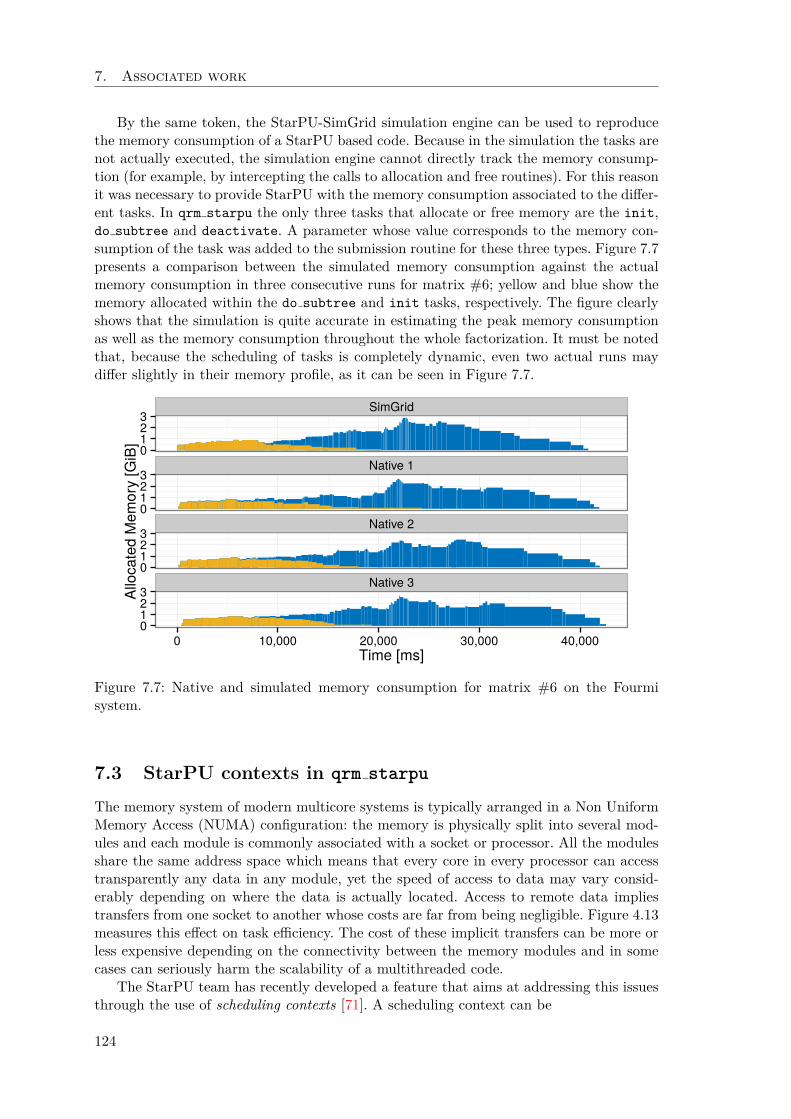
7. Associated work

By the same token, the StarPU-SimGrid simulation engine can be used to reproducethe memory consumption of a StarPU based code. Because in the simulation the tasks arenot actually executed, the simulation engine cannot directly track the memory consump-tion (for example, by intercepting the calls to allocation and free routines). For this reasonit was necessary to provide StarPU with the memory consumption associated to the differ-ent tasks. In qrm starpu the only three tasks that allocate or free memory are the init,do subtree and deactivate. A parameter whose value corresponds to the memory con-sumption of the task was added to the submission routine for these three types. Figure 7.7presents a comparison between the simulated memory consumption against the actualmemory consumption in three consecutive runs for matrix #6; yellow and blue show thememory allocated within the do subtree and init tasks, respectively. The figure clearlyshows that the simulation is quite accurate in estimating the peak memory consumptionas well as the memory consumption throughout the whole factorization. It must be notedthat, because the scheduling of tasks is completely dynamic, even two actual runs maydiffer slightly in their memory profile, as it can be seen in Figure 7.7.

Native 2

Native 3

0123

Native 1

0123

SimGrid

0123

0123

0 10,000 20,000 30,000 40,000

Time [ms]

Allo

ca

ted

Me

mo

ry [

GiB

]

Figure 7.7: Native and simulated memory consumption for matrix #6 on the Fourmisystem.

7.3 StarPU contexts in qrm starpu

The memory system of modern multicore systems is typically arranged in a Non UniformMemory Access (NUMA) configuration: the memory is physically split into several mod-ules and each module is commonly associated with a socket or processor. All the modulesshare the same address space which means that every core in every processor can accesstransparently any data in any module, yet the speed of access to data may vary consid-erably depending on where the data is actually located. Access to remote data impliestransfers from one socket to another whose costs are far from being negligible. Figure 4.13measures this effect on task efficiency. The cost of these implicit transfers can be more orless expensive depending on the connectivity between the memory modules and in somecases can seriously harm the scalability of a multithreaded code.

The StarPU team has recently developed a feature that aims at addressing this issuesthrough the use of scheduling contexts [71]. A scheduling context can be

124

7.3. StarPU contexts in qrm starpu

defined as a structure able to encapsulate a parallel code and restrict its ex-ecution on a section of the machine. By means of the scheduling contexts, aparallel code runs on top of an abstract machine, whose set of resources canbe dynamically changed during its execution. This allows the programmers tocontrol the distribution of computing resources (i.e. CPUs and GPUs) overco-executing parallel kernels (Hugo [72])

Scheduling contexts can be used for efficiently composing StarPU based applications.Imagine a scenario where two applications have to be executed concurrently on the samemachine. Two contexts can be created, one for each application, and each of them can beassigned an amount of resources (e.g., processing units) proportional to the relative weightof the associated application; all the tasks related to one application will be submitted to,and handled by the corresponding scheduling context and, as a consequence, executed bythe associated resources. This will prevent the two applications from interfering with eachother (for example polluting each others caches) and from competing for resources.

Scheduling contexts were later used to improve the scalability of qrm starpu on NUMAarchitectures by Hugo et al. [70]. This idea stems from the observation that separatebranches of the elimination tree are independent and can thus be assigned to differentcontexts including disjoint subsets of resources whose size is established depending ontheir relative weight. Resources within each context share some level of memory (e.g.,cache or NUMA module), which allows the reduction the cache miss rate or the transferof data among NUMA modules and thus improves performance.

The analysis phase of the qrm starpu solver has been extended with a proportionalmapping [92] step. This algorithm consists in a top-down traversal: all the available re-sources are mapped on the root node of the elimination tree and then they are partitionedinto bundles and each bundle assigned to a set of child nodes. The amount of resourcesin each bundle depends on the relative weight of the subtrees rooted at the child nodes.This process is applied recursively until all the bundles contain a minimum, non divisibleamount of resources (for instance, one core). The weight of each subtree can be computedas the time needed to process the entire subtree, according to a given performance model.Each bundle is then mapped to context. This results in a tree of contexts which matchesthe memory hierarchy as shown in Figure 7.8: all the resources in a context/bundle sharesome level of memory (say, L2 cache) and all those in the higher level context, obtainedby merging all the contexts in a set of siblings, share a lower level memory (L3 cache).

L3

L2

Module

Figure 7.8: Mapping of tree nodes to contexts.

Note that the initial mapping of resources may be inaccurate due to inaccuracies of theperformance model or because it cannot take into account conditions that are related to theload of the machine. In order to address this issue a hypervisor process constantly monitors

125

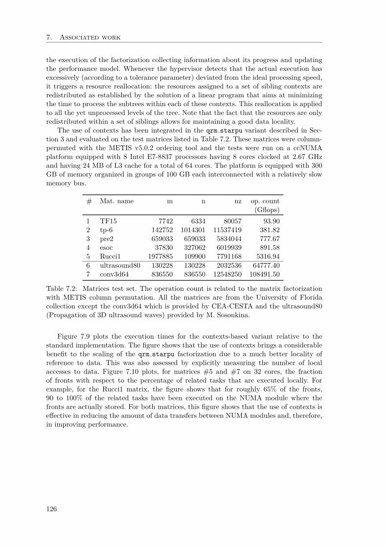
7. Associated work

the execution of the factorization collecting information about its progress and updatingthe performance model. Whenever the hypervisor detects that the actual execution hasexcessively (according to a tolerance parameter) deviated from the ideal processing speed,it triggers a resource reallocation: the resources assigned to a set of sibling contexts areredistributed as established by the solution of a linear program that aims at minimizingthe time to process the subtrees within each of these contexts. This reallocation is appliedto all the yet unprocessed levels of the tree. Note that the fact that the resources are onlyredistributed within a set of siblings allows for maintaining a good data locality.

The use of contexts has been integrated in the qrm starpu variant described in Sec-tion 3 and evaluated on the test matrices listed in Table 7.2. These matrices were column-permuted with the METIS v5.0.2 ordering tool and the tests were run on a ccNUMAplatform equipped with 8 Intel E7-8837 processors having 8 cores clocked at 2.67 GHzand having 24 MB of L3 cache for a total of 64 cores. The platform is equipped with 300GB of memory organized in groups of 100 GB each interconnected with a relatively slowmemory bus.

# Mat. name m n nz op. count(Gflops)

1 TF15 7742 6334 80057 93.902 tp-6 142752 1014301 11537419 381.823 pre2 659033 659033 5834044 777.674 esoc 37830 327062 6019939 891.585 Rucci1 1977885 109900 7791168 5316.94

6 ultrasound80 130228 130228 2032536 64777.407 conv3d64 836550 836550 12548250 108491.50

Table 7.2: Matrices test set. The operation count is related to the matrix factorizationwith METIS column permutation. All the matrices are from the University of Floridacollection except the conv3d64 which is provided by CEA-CESTA and the ultrasound80(Propagation of 3D ultrasound waves) provided by M. Sosonkina.

Figure 7.9 plots the execution times for the contexts-based variant relative to thestandard implementation. The figure shows that the use of contexts brings a considerablebenefit to the scaling of the qrm starpu factorization due to a much better locality ofreference to data. This was also assessed by explicitly measuring the number of localaccesses to data. Figure 7.10 plots, for matrices #5 and #7 on 32 cores, the fractionof fronts with respect to the percentage of related tasks that are executed locally. Forexample, for the Rucci1 matrix, the figure shows that for roughly 65% of the fronts,90 to 100% of the related tasks have been executed on the NUMA module where thefronts are actually stored. For both matrices, this figure shows that the use of contexts iseffective in reducing the amount of data transfers between NUMA modules and, therefore,in improving performance.

126

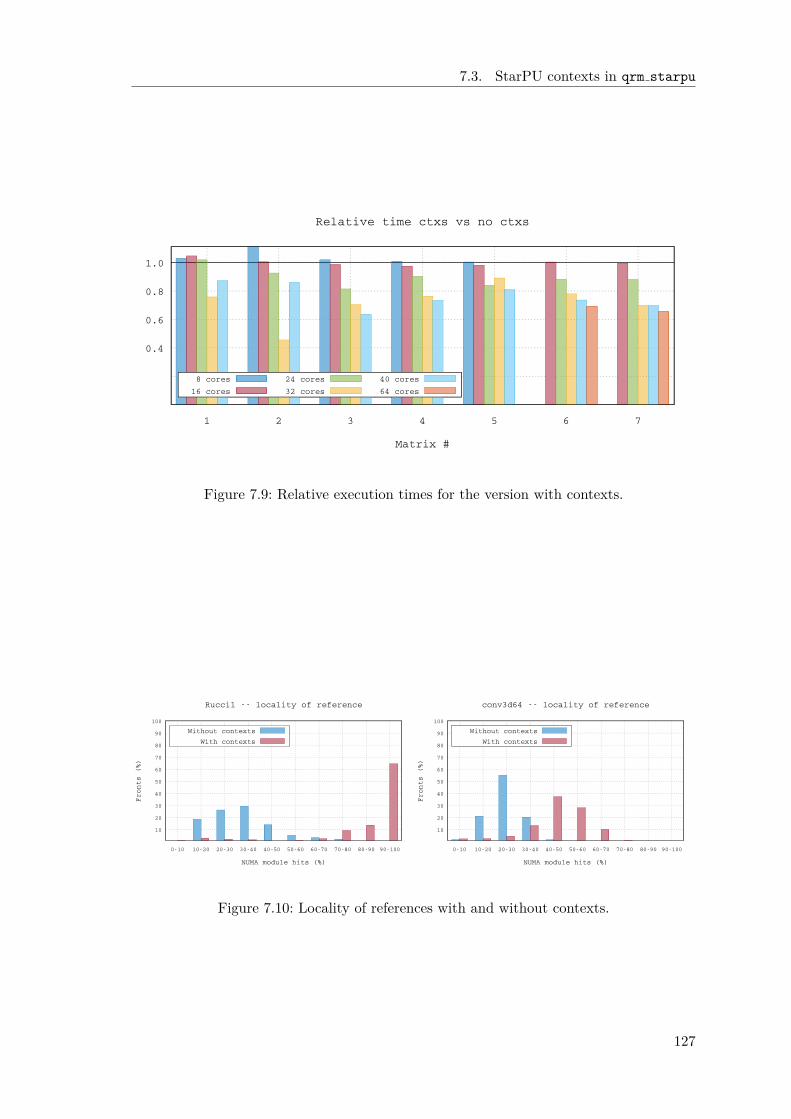
7.3. StarPU contexts in qrm starpu

0.4

0.6

0.8

1.0

1 2 3 4 5 6 7

Matrix #

Relative time ctxs vs no ctxs

8 cores

16 cores

24 cores

32 cores

40 cores

64 cores

Figure 7.9: Relative execution times for the version with contexts.

10

20

30

40

50

60

70

80

90

100

0-10 10-20 20-30 30-40 40-50 50-60 60-70 70-80 80-90 90-100

Fronts (%)

NUMA module hits (%)

Rucci1 -- locality of reference

Without contexts

With contexts

10

20

30

40

50

60

70

80

90

100

0-10 10-20 20-30 30-40 40-50 50-60 60-70 70-80 80-90 90-100

Fronts (%)

NUMA module hits (%)

conv3d64 -- locality of reference

Without contexts

With contexts

Figure 7.10: Locality of references with and without contexts.

127

Chapter 8

Conclusion

8.1 General conclusion

In this thesis we have addressed the design of a sparse direct solver, capable of efficientlyexploiting multicore and heterogeneous architectures, using modern runtime systems.

The first issue we addressed in Chapter 3 is to prove the relevance of our approach byporting the multifrontal method implemented in qr mumps on top of StarPU. In this chap-ter the StarPU based version of qr mumps, referred to as qrm starpu, is experimentallyvalidated by performing a comparative study with the original solver which, essentially,assesses the validity of the approach and the usability of runtime systems for the imple-mentation of sparse, direct methods.

Although capable of achieving good performance this implementation relies on a mix-ture of parallel programming models (see Section 1.4.1) which constitutes a hindranceto the development of new features. For this reason, we redesigned the implementationqrm starpu using a pure Sequential Task Flow model. In Chapter 4, we first presented aSTF-parallelization of the multifrontal method using the original 1D block-column par-titioning scheme (the same as in the qr mumps solver and in the approach described inChapter 3), showed the expressiveness and simplicity of use of this parallel programmingmodel and proved the efficiency of the resulting code. Based on this, we improved thesolver by integrating 2D communication avoiding front factorization algorithms and showhow this is relatively easy to implement, thanks to simplicity of the programming model.The superior performance and scalability of the resulting solver is assessed through a richset of experimental results and a finely detailed performance analysis. Furthermore wedeveloped and present in Chapter 5 a memory-aware algorithm which allows us to controlthe memory consumption of the parallel multifrontal method. We showed on a set of testmatrices that we were able to obtain the same performance results as the non constrainedcase when enforcing a memory limit equal to the minimal memory consumption associatedwith the sequential algorithm.

In compliance with the STF parallel programming model, we moved forward to het-erogeneous architectures in Chapter 6 and addressed the data partitioning and schedulingissues that are critical to achieve performance on these architectures. We extended the1D block-column partitioning into a hierarchical block partitioning allowing to generateboth fine and coarse granularity tasks suited to the processing unit capabilities. We de-velop a scheduling strategy capable of handling the task heterogeneity in the DAG andthe diversity of resources on heterogeneous architectures. A performance analysis on aset of test matrices indicates that we are capable of efficiently exploiting heterogeneousarchitectures.

129

8. Conclusion

The validity and efficiency of all the methods presented in this thesis are assessedthrough experimental results. Considering the complexity of algorithms and computerarchitectures, this challenged us with the difficulty of profiling and analysing the per-formance of our implementations as well as the difficulty of identifying and quantifyingpotential sources of inefficiency. For this purpose, we developed a performance analysisapproach, presented in Chapter 2, capable of measuring and separately analysing severalfactors that play a role in performance and scalability such as locality issues and taskpipelining. Additionally, this analysis allows us to measure the cost of the runtime systemand thus provides a further proof of the efficiency and usability of these tools.

Finally we presented in Chapter 7 some collaborative work done in the context ofqrm starpu. First we implemented another version of qr mumps using an alternative pro-gramming model, namely a parametrized task graph. Then we focused on reproducingand simulating parallel executions in qrm starpu. Lastly, we briefly presented the use ofscheduling contexts with StarPU that enhances the exploitation of data locality in themultifrontal method.

Although our work clearly benefited from the features, the performance and the re-liability of modern runtime systems, it must be noted that it also provided a valuablefeedback to the developers of these tools. The results achieved by our work led to the de-velopment and implementation of novel features within the StarPU runtime system suchas commutable tasks, dynamic partitioning/unpartitioning tasks and methods for guidingthe submission of tasks based on the memory consumption.

8.2 Perspectives and future work

The work achieved in this thesis opens up a large number of opportunities for futuredevelopments both from an algorithmic (novel methods and algorithms for improving theperformance and reliability of the solver) and from the software performance optimizationpoints of view.

In our study on heterogeneous architectures, we presented experimental results onGPU-accelerated architectures. We believe that the strategies that we have developed toexploit these architectures can be used to exploit systems equipped with other types ofaccelerators such as the Intel Xeon Phi coprocessors. The techniques that we proposed aredesigned for heterogeneous architectures in general and thus are independent from GPUs.The algorithms that we presented are implemented using a high-level programming modelwhile the runtime system handles the underlying architecture. Provided that we give thespecific kernels to the runtime system, we should be able to exploit Xeon Phi-acceleratedarchitectures.

Thanks to the runtime system approach, the current version of qrm starpu is capableof exploiting multiple GPUs. However it is unlikely to have good performance because itdoes not address potential problems coming from GPU-to-GPU data transfers. Therefore,we need to address data locality issues by developing an appropriate scheduling policy.

In this thesis we focused on single node, multicore and heterogeneous architectures al-though modern runtime systems like StarPU and PaRSEC are capable of using distributed-memory architectures. Implementing the multifrontal QR factorization on such systemsrepresents a hard challenge and requires special care in developing appropriate data dis-tribution and mapping as well as tasks scheduling methods in order to minimize the costof data transfers through the network that connects the nodes of the system.

The qrm starpu solver developed in this thesis provides a reliable and efficient platformfor algorithmic developments and opens up opportunities for developing novel numerical

130

8.2. Perspectives and future work

methods with a relatively limited implementation effort.The performance of the methods presented in this thesis, depends on the value of a

number of parameters, most notably the block-sizes for either the 1D, 2D or hierarchicalfronts partitioning. In the experimental results presented in the previous chapters, wesimply tested a range of values for each of these parameters and only reported performancefor the best cases. Nonetheless, it should be possible to automatically select the valuesthat yield optimal or close to optimal performance depending on the properties of theworkload (shape of the elimination tree and/or of the DAG, granularity of tasks, shapeand size of the frontal matrices) and the machine (number and type of processing units,speed of memory, performance of BLAS routines). This is an extremely challenging taskto achieve but may lead to a much better ease of use of the qrm starpu solver. Moreover,it should be noted that the value of these blocking sizes does not have to be the same forall the frontal matrices in the elimination tree. For example, at the bottom of the tree,where much tree parallelism is available, node parallelism can be reduced by choosinglarger block sizes or even a 1D partitioning in order to improve the efficiency of singletasks. By the same token, the panel reduction method in 2D factorization algorithms,may be chosen depending on the shape of every single front. This is clearly a very difficultchallenge to tackle but may lead to considerable performance improvements.

One critical task we plan to pursue in future work is the extension of the qrm starpu

solver to support rank-deficient systems. Techniques like the Heath [63] method (also usedin the spqr solver) can be employed to handle this type of problem and possibly be im-proved through the use of restricted pivoting techniques. It must be noted, though, thatthese techniques require special care in the task submission and scheduling. The detectionof rank deficiency within a frontal matrix implies modifications of the structure of its an-cestors (potentially up to the root of the elimination tree). Because rank deficiencies canonly be detected during the matrix factorization, it is not possible to submit the wholeDAG solely relying on the information from the symbolic analysis phase. The submissionof some tasks is subordinated to the result of previous ones and therefore the DAG dy-namically changes at runtime. Special strategies must be designed and implemented tocope with this issue.

Regarding the extremely good performance results obtained with our memory-awarealgorithm in qrm starpu, it should be noted that our approach is very conservative interms of memory and may limit the exploitation of tree parallelism which could severelyreduce the scalability of our solver on larger scale platforms. In addition, the proposedalgorithm is especially suited to the multifrontal QR factorization for the reasons thatwe enumerated in our study and might not be as efficient in the context of other typesof multifrontal methods. We could thus refine our algorithm with strategies such as thememory booking heuristics proposed by Eyraud-Dubois et al. [50].

This thesis essentially focused on the factorization of a sparse matrix. As explainedin the introduction, this is only one of the three main phases of a sparse direct solver.The factorization is commonly followed by one or more solve operations with one or moreright-hand sides. Although all the techniques presented in this thesis can readily be appliedto the solve phase, it must be noted that in the case of a single right-hand side the solvephase becomes memory-bound. This means that the relative weight of tasks is very small(much smaller than in the factorization phase) and therefore the runtime overhead is likelyto increase. A different parallelization scheme may have to be employed in this case toovercome this issue. As for the analysis, no floating-point computations are performed inthe various steps of this analysis which are all, inherently, memory bound. Although thisphase is relatively light with respect to the factorization and the solve, its weight becomesmore significant as these are accelerated by exploiting parallelism. The use of runtime

131

8. Conclusion

systems for parallelizing the analysis phase may be challenging due to the nature of theoperations performed therein.

132

Submitted articles

Publications

Submitted articles

[S1] E. Agullo, A. Buttari, A. Guermouche, and F. Lopez. Implementing multifrontalsparse solvers for multicore architectures with Sequential Task Flow runtime sys-tems. Tech. rep. IRI/RT–2014-03–FR. Submitted to ACM Transactions On Math-ematical Software. IRIT, Nov. 2014. url: http://buttari.perso.enseeiht.fr/

stuff/IRI-RT--2014-03--FR.pdf.

Conference proceedings

[C1] E. Agullo, A. Buttari, A. Guermouche, and F. Lopez. “Multifrontal QR Factoriza-tion for Multicore Architectures over Runtime Systems”. In: Euro-Par 2013 ParallelProcessing. Springer Berlin Heidelberg, 2013, pp. 521–532. isbn: 978-3-642-40046-9.url: http://dx.doi.org/10.1007/978-3-642-40047-6_53.

[C2] E. Agullo, A. Buttari, A. Guermouche, and F. Lopez. Task-based multifrontal QRsolver for GPU-accelerated multicore architectures. Tech. rep. IRI/RT–2015–02–FR. Accepted at the HiPC 2015 conference. IRIT, June 2015. url: https://hal.

archives-ouvertes.fr/hal-01166312v2.

Posters

[P1] E. Agullo et al. Matrices Over Runtime Systems at Exascale. Poster at the Super-Computing 2015 conference. 2015.

Conference talks

[T1] E. Agullo, A. Buttari, A. Guermouche, and F. Lopez. Multifrontal QR Factorizationfor Multicore Architectures over Runtime Systems. Presentation at the Euro-Par2013 international conference, Aachen August 26-30 2013. 2013.

[T2] E. Agullo, A. Buttari, A. Guermouche, and F. Lopez. Sparse direct solvers on topof a runtime system. Presentation at the PMAA 2014 international conference,Lugano July 2-4 2014. 2014.

[T3] E. Agullo, A. Buttari, A. Guermouche, and F. Lopez. Sparse direct solvers ontop of a runtime system. Presentation at the SIAM Computational Science andEngineering international conference, Salt Lake City, March 14-18 2015. 2015.

[T4] E. Agullo, A. Buttari, A. Guermouche, and F. Lopez. Task-based multifrontal QRsolver for GPU-accelerated multicore architectures. Presentation at the Sparse Daysin St Girons international conference, St Girons, June 29 - July 2 2015. 2015.

[T5] A. Decollas and F. Lopez. Direct methods on GPU-based systems, preliminary worktowards a functioning code. Presentation at the Sparse Days workshop, Toulouse,June 2012. 2012.

133

References

[1] E. Agullo. “On the out-of-core factorization of large sparse matrices”. PhD thesis.Ecole Normale Superieure de Lyon, Nov. 2008.

[2] E. Agullo, P. R. Amestoy, A. Buttari, A. Guermouche, J.-Y. L’Excellent, andF.-H. Rouet. Robust memory-aware mappings for parallel multifrontal factoriza-tions. Submitted to SIAM SISC. 2012.

[3] E. Agullo, C. Augonnet, J. Dongarra, M. Faverge, J. Langou, H. Ltaief, and S. To-mov. “LU factorization for accelerator-based systems”. In: AICCSA. 2011, pp. 217–224. doi: http://dx.doi.org/10.1109/AICCSA.2011.6126599.

[4] E. Agullo, C. Augonnet, J. Dongarra, M. Faverge, H. Ltaief, S. Thibault, and S. To-mov. “QR Factorization on a Multicore Node Enhanced with Multiple GPU Accel-erators”. In: Proceedings of 25th International Parallel and Distributed ProcessingSymposium (IPDPS’11). 2011, pp. 932–943. doi: http://doi.ieeecomputersociety.

org/10.1109/IPDPS.2011.90.

[5] E. Agullo, C. Augonnet, J. Dongarra, H. Ltaief, R. Namyst, S. Thibault, and S.Tomov. “A Hybridization Methodology for High-Performance Linear Algebra Soft-ware for GPUs”. In: in GPU Computing Gems, Jade Edition 2 (2011), pp. 473–484.

[6] E. Agullo, O. Beaumont, L. Eyraud-Dubois, J. Herrmann, S. Kumar, L. Marchal,and S. Thibault. “Bridging the Gap between Performance and Bounds of CholeskyFactorization on Heterogeneous Platforms”. In: Heterogeneity in Computing Work-shop 2015. Hyderabad, India, May 2015. url: https://hal.inria.fr/hal-

01120507.

[7] E. Agullo, B. Bramas, O. Coulaud, E. Darve, M. Messner, and T. Takahashi. Task-based FMM for heterogeneous architectures. Research Report RR-8513. Inria, Apr.2014, p. 29. url: https://hal.inria.fr/hal-00974674.

[8] E. Agullo, C. Coti, J. Dongarra, T. Herault, and J. Langou. “QR factorization oftall and skinny matrices in a grid computing environment”. In: Parallel DistributedProcessing (IPDPS), 2010 IEEE International Symposium on. Apr. 2010, pp. 1–11.doi: 10.1109/IPDPS.2010.5470475.

[9] E. Agullo, J. Demmel, J. Dongarra, B. Hadri, J. Kurzak, J. Langou, H. Ltaief, P.Luszczek, and S. Tomov. “Numerical linear algebra on emerging architectures: ThePLASMA and MAGMA projects”. In: Journal of Physics: Conference Series 180.1(2009), p. 012037. url: http://stacks.iop.org/1742-6596/180/i=1/a=012037.

[10] E. Agullo, J. Dongarra, R. Nath, and S. Tomov. “Fully Empirical Autotuned QRFactorization For Multicore Architectures”. In: CoRR abs/1102.5328 (2011).

[11] R. Allen and K. Kennedy. Optimizing Compilers for Modern Architectures: ADependence-Based Approach. Morgan Kaufmann, 2002.

135

References

[12] P. R. Amestoy, T. A. Davis, and I. S. Duff. “Algorithm 837: AMD, an approxi-mate minimum degree ordering algorithm”. In: ACM Transactions On Mathemat-ical Software 33(3) (2004), pp. 381–388.

[13] P. R. Amestoy, I. S. Duff, J. Koster, and J.-Y. L’Excellent. “MUMPS: a generalpurpose distributed memory sparse solver”. In: Proceedings of PARA2000, the FifthInternational Workshop on Applied Parallel Computing, Bergen, June 18-21. Ed. byA. H. Gebremedhin, F. Manne, R. Moe, and T. Sørevik. Lecture Notes in ComputerScience 1947. Springer-Verlag, 2000, pp. 122–131.

[14] P. R. Amestoy, I. S. Duff, and C. Puglisi. “Multifrontal QR factorization in amultiprocessor environment”. In: Int. Journal of Num. Linear Alg. and Appl. 3(4)(1996), pp. 275–300.

[15] E. Anderson et al. LAPACK Users’ Guide. Third. Philadelphia, PA: Society forIndustrial and Applied Mathematics, 1999. isbn: 0-89871-447-8 (paperback).

[16] M. Anderson, G. Ballard, J. Demmel, and K. Keutzer. “Communication-AvoidingQR Decomposition for GPUs”. In: Proceedings of the 2011 IEEE InternationalParallel & Distributed Processing Symposium. IPDPS ’11. Washington, DC, USA:IEEE Computer Society, 2011, pp. 48–58. isbn: 978-0-7695-4385-7. doi: 10.1109/

IPDPS.2011.15. url: http://dx.doi.org/10.1109/IPDPS.2011.15.

[17] K. Asanovic et al. The Landscape of Parallel Computing Research: A View fromBerkeley. Tech. rep. UCB/EECS-2006-183. TECHNICAL REPORT, UC BERKE-LEY, 2006.

[18] C. Augonnet, S. Thibault, R. Namyst, and P.-A. Wacrenier. “StarPU: A UnifiedPlatform for Task Scheduling on Heterogeneous Multicore Architectures”. In: Con-currency and Computation: Practice and Experience, Special Issue: Euro-Par 200923 (2 Feb. 2011), pp. 187–198. doi: 10.1002/cpe.1631. url: http://hal.inria.

fr/inria-00550877.

[19] E. Ayguade, R. M. Badia, F. D. Igual, J. Labarta, R. Mayo, and E. S. Quintana-Ortı. “An Extension of the StarSs Programming Model for Platforms with MultipleGPUs”. In: Euro-Par. 2009, pp. 851–862. doi: 10.1007/978-3-642-03869-3_79.

[20] R. M. Badia, J. R. Herrero, J. Labarta, J. M. Perez, E. S. Quintana-Ortı, andG. Quintana-Ortı. “Parallelizing dense and banded linear algebra libraries usingSMPSs”. In: Concurrency and Computation: Practice and Experience 21.18 (2009),pp. 2438–2456.

[21] G. Ballard, E. Carson, J. Demmel, M. Hoemmen, N. Knight, and O. Schwartz.“Communication lower bounds and optimal algorithms for numerical linear alge-bra”. In: Acta Numerica 23 (May 2014), pp. 1–155. issn: 1474-0508. doi: 10 .

1017/S0962492914000038. url: http://journals.cambridge.org/article_

S0962492914000038.

[22] G. Ballard, J. Demmel, O. Holtz, and O. Schwartz. “Minimizing Communication inNumerical Linear Algebra”. In: SIAM Journal on Matrix Analysis and Applications32.3 (2011), pp. 866–901. doi: 10.1137/090769156. eprint: http://dx.doi.org/

10.1137/090769156. url: http://dx.doi.org/10.1137/090769156.

[23] A. Bjorck. Numerical methods for Least Squares Problems. Philadelphia: SIAM,1996.

[24] T. O. architecture review board. OpenMP 4.0 Complete specifications. 2013.

136

References

[25] G. Bosilca, A. Bouteiller, A. Danalis, M. Faverge, T. Herault, and J. J. Dongarra.“PaRSEC: Exploiting Heterogeneity to Enhance Scalability”. In: Computing inScience and Engineering 15.6 (2013), pp. 36–45. doi: 10.1109/MCSE.2013.98.url: http://dx.doi.org/10.1109/MCSE.2013.98.

[26] G. Bosilca, A. Bouteiller, A. Danalis, T. Herault, P. Lemarinier, and J. Dongarra.“DAGuE: A generic distributed DAG engine for High Performance Computing”.In: Parallel Computing 38.1-2 (2012), pp. 37–51. doi: 10.1016/j.parco.2011.

10.003.

[27] G. Bosilca, A. Bouteiller, A. Danalis, T. Herault, P. Luszczek, and J. Dongarra.“Dense Linear Algebra on Distributed Heterogeneous Hardware with a SymbolicDAG Approach”. In: Scalable Computing and Communications: Theory and Prac-tice (2013), pp. 699–733.

[28] G. Bosilca et al. “Distibuted Dense Numerical Linear Algebra Algorithms on mas-sively parallel architectures: DPLASMA”. In: Proceedings of the 25th IEEE Inter-national Symposium on Parallel and Distributed Processing Workshops and Phd Fo-rum (IPDPSW’11), PDSEC 2011. Anchorage, United States, May 2011, pp. 1432–1441. url: https://hal.inria.fr/hal-00809680.

[29] H. Bouwmeester, M. Jacquelin, J. Langou, and Y. Robert. “Tiled QR Factoriza-tion Algorithms”. In: Proceedings of 2011 International Conference for High Perfor-mance Computing, Networking, Storage and Analysis. SC ’11. Seattle, Washington:ACM, 2011, 7:1–7:11. isbn: 978-1-4503-0771-0. doi: 10.1145/2063384.2063393.url: http://doi.acm.org/10.1145/2063384.2063393.

[30] F. Broquedis, J. Clet-Ortega, S. Moreaud, N. Furmento, B. Goglin, G. Mercier, S.Thibault, and R. Namyst. “hwloc: A Generic Framework for Managing HardwareAffinities in HPC Application”. In: Parallel, Distributed and Network-Based Pro-cessing (PDP), 2010 18th Euromicro International Conference. Feb. 2010, pp. 180–186. doi: 10.1109/PDP.2010.67.

[31] A. Buttari. “Fine granularity sparse QR factorization for multicore based systems”.In: Proceedings of the 10th international conference on Applied Parallel and Scien-tific Computing - Volume 2. PARA’10. Reykjavik, Iceland: Springer-Verlag, 2012,pp. 226–236. isbn: 978-3-642-28144-0. url: http://dx.doi.org/10.1007/978-

3-642-28145-7_23.

[32] A. Buttari. “Fine-Grained Multithreading for the Multifrontal QR Factorization ofSparse Matrices”. In: SIAM Journal on Scientific Computing 35.4 (2013), pp. C323–C345. eprint: http://epubs.siam.org/doi/pdf/10.1137/110846427. url:http://epubs.siam.org/doi/abs/10.1137/110846427.

[33] A. Buttari, J. Dongarra, J. Kurzak, J. Langou, P. Luszczek, and S. Tomov. “Theimpact of multicore on math software”. In: Proceedings of the 8th internationalconference on Applied parallel computing: state of the art in scientific computing.PARA’06. Umea;, Sweden: Springer-Verlag, 2007, pp. 1–10. isbn: 3-540-75754-6,978-3-540-75754-2. url: http : / / dl . acm . org / citation . cfm ? id = 1775059 .

1775061.

[34] A. Buttari, J. Langou, J. Kurzak, and J. Dongarra. “A class of parallel tiled linearalgebra algorithms for multicore architectures”. In: Parallel Comput. 35 (1 Jan.2009), pp. 38–53. issn: 0167-8191. doi: 10.1016/j.parco.2008.10.002. url:http://dl.acm.org/citation.cfm?id=1486274.1486415.

137

References

[35] A. Buttari, J. Langou, J. Kurzak, and J. Dongarra. “Parallel tiled QR factorizationfor multicore architectures”. In: Concurr. Comput. : Pract. Exper. 20.13 (2008),pp. 1573–1590. issn: 1532-0626. doi: 10.1002/cpe.v20:13.

[36] H. Casanova, A. Giersch, A. Legrand, M. Quinson, and F. Suter. “Versatile, Scal-able, and Accurate Simulation of Distributed Applications and Platforms”. Anglais.In: Journal of Parallel and Distributed Computing 74.10 (June 2014), pp. 2899–2917. doi: 10.1016/j.jpdc.2014.06.008.

[37] E. Chan, F. G. V. Zee, P. Bientinesi, E. S. Quintana-Ortı, G. Quintana-Ortı, andR. A. van de Geijn. “SuperMatrix: a multithreaded runtime scheduling system foralgorithms-by-blocks”. In: PPOPP. 2008, pp. 123–132.

[38] M. Cosnard and M. Loi. “Automatic task graph generation techniques”. In: SystemSciences, 1995. Proceedings of the Twenty-Eighth Hawaii International Conferenceon. Vol. 2. Jan. 1995, 113–122 vol.2. doi: 10.1109/HICSS.1995.375471.

[39] E. J. Craig. “The N-step iteration procedures”. In: Journal of Mathematics andPhysics 34 (1955), pp. 64–73.

[40] T. A. Davis, J. R. Gilbert, S. I. Larimore, and E. G. Ng. “A column approximateminimum degree ordering algorithm”. In: ACM Trans. Math. Softw. 30.3 (Sept.2004), pp. 353–376. issn: 0098-3500. doi: 10.1145/1024074.1024079. url: http:

//doi.acm.org/10.1145/1024074.1024079.

[41] T. Davis. Direct Methods for Sparse Linear Systems. Society for Industrial andApplied Mathematics, 2006. doi: 10.1137/1.9780898718881. eprint: http://

epubs.siam.org/doi/pdf/10.1137/1.9780898718881. url: http://epubs.

siam.org/doi/abs/10.1137/1.9780898718881.

[42] T. A. Davis. “Algorithm 915, SuiteSparseQR: Multifrontal multithreaded rank-revealing sparse QR factorization”. In: ACM Trans. Math. Softw. 38.1 (Dec. 2011),8:1–8:22. issn: 0098-3500. doi: 10.1145/2049662.2049670. url: http://doi.

acm.org/10.1145/2049662.2049670.

[43] T. A. Davis and Y. Hu. “The university of Florida sparse matrix collection”. In:ACM Trans. Math. Softw. 38.1 (Dec. 2011), 1:1–1:25. issn: 0098-3500. url: http:

//doi.acm.org/10.1145/2049662.2049663.

[44] J. Demmel, L. Grigori, M. Hoemmen, and J. Langou. “Communication-optimalParallel and Sequential QR and LU Factorizations”. In: SIAM J. Sci. Comput.34.1 (Feb. 2012), pp. 206–239. issn: 1064-8275. url: http://dx.doi.org/10.

1137/080731992.

[45] E. W. Dijkstra. “Een algorithme ter voorkoming van de dodelijke omarming”. cir-culated privately. 1965. url: http://www.cs.utexas.edu/users/EWD/ewd01xx/

EWD108.PDF.

[46] E. W. Dijkstra. “The Mathematics Behind the Banker’s Algorithm”. English. In:Selected Writings on Computing: A personal Perspective. Texts and Monographs inComputer Science. Springer New York, 1982, pp. 308–312. isbn: 978-1-4612-5697-7.doi: 10.1007/978-1-4612-5695-3_54. url: http://dx.doi.org/10.1007/978-

1-4612-5695-3_54.

[47] J. Dongarra, M. Faverge, T. Herault, M. Jacquelin, J. Langou, and Y. Robert. “Hi-erarchical QR factorization algorithms for multi-core clusters”. In: Parallel Com-puting 39.4-5 (2013), pp. 212–232. url: http://hal.inria.fr/hal-00809770.

138

References

[48] I. S. Duff, A. M. Erisman, and J. K. Reid. Direct Methods for Sparse Matrices.New York, NY, USA: Oxford University Press, Inc., 1986. isbn: 0-198-53408-6.

[49] I. S. Duff and J. K. Reid. “The multifrontal solution of indefinite sparse symmet-ric linear systems”. In: ACM Transactions On Mathematical Software 9 (1983),pp. 302–325.

[50] L. Eyraud-Dubois, L. Marchal, O. Sinnen, and F. Vivien. “Parallel Scheduling ofTask Trees with Limited Memory”. In: ACM Trans. Parallel Comput. 2.2 (June2015), 13:1–13:37. issn: 2329-4949. doi: 10.1145/2779052. url: http://doi.

acm.org/10.1145/2779052.

[51] L. Eyraud-Dubois, L. Marchal, O. Sinnen, and F. Vivien. “Parallel scheduling oftask trees with limited memory”. In: CoRR abs/1410.0329 (2014). url: http:

//arxiv.org/abs/1410.0329.

[52] M. Garland, S. L. Grand, J. Nickolls, J. Anderson, J. Hardwick, S. Morton, E.Phillips, Y. Zhang, and V. Volkov. “Parallel Computing Experiences with CUDA”.In: IEEE Micro 28.4 (2008), pp. 13–27.

[53] T. Gautier, F. Le Mentec, V. Faucher, and B. Raffin. “X-kaapi: A Multi ParadigmRuntime for Multicore Architectures”. In: 42nd International Conference on Par-allel Processing, ICPP 2013, Lyon, France, October 1-4, 2013. 2013, pp. 728–735.doi: 10.1109/ICPP.2013.86. url: http://dx.doi.org/10.1109/ICPP.2013.86.

[54] A. Geist and E. G. Ng. “Task scheduling for parallel sparse Cholesky factorization”.In: Int J. Parallel Programming 18 (1989), pp. 291–314.

[55] A. J. George. “Nested dissection of a regular finite-element mesh”. In: SIAM J.Numer. Anal. 10.2 (1973), pp. 345–363.

[56] T. George, V. Saxena, A. Gupta, A. Singh, and A. R. Choudhury. “MultifrontalFactorization of Sparse SPD Matrices on GPUs”. In: Proceedings of 25th Interna-tional Parallel and Distributed Processing Symposium (IPDPS’11). 2011, pp. 372–383.

[57] W. Givens. “Computation of Plane Unitary Rotations Transforming a GeneralMatrix to Triangular Form”. English. In: Journal of the Society for Industrial andApplied Mathematics 6.1 (1958), pp. 26–50. issn: 03684245. url: http://www.

jstor.org/stable/2098861.

[58] G. Golub. “Numerical methods for solving linear least squares problems”. English.In: Numerische Mathematik 7.3 (1965), pp. 206–216. issn: 0029-599X. doi: 10.

1007/BF01436075. url: http://dx.doi.org/10.1007/BF01436075.

[59] G. H. Golub and C. F. Van Loan. Matrix Computations. 4th ed. Baltimore, MD.:Johns Hopkins Press, 2012.

[60] A. Guermouche, J.-Y. L’Excellent, and G. Utard. “Impact of Reordering on theMemory of a Multifrontal Solver”. In: Parallel Computing 29.9 (2003), pp. 1191–1218.

[61] B. Hadri, H. Ltaief, E. Agullo, and J. Dongarra. “Tile QR factorization with parallelpanel processing for multicore architectures”. In: IPDPS. IEEE, 2010, pp. 1–10.url: http://dx.doi.org/10.1109/IPDPS.2010.5470443.

[62] T. D. R. Hartley, E. Saule, and U. V. Catalyurek. “Improving performance ofadaptive component-based dataflow middleware”. In: Parallel Computing 38.6-7(2012), pp. 289–309.

139

References

[63] M. T. Heath. “Some Extensions of an Algorithm for Sparse Linear Least SquaresProblems”. In: SIAM Journal on Scientific and Statistical Computing 3.2 (1982),pp. 223–237. doi: 10.1137/0903014. eprint: http://dx.doi.org/10.1137/

0903014. url: http://dx.doi.org/10.1137/0903014.

[64] P. Henon, P. Ramet, and J. Roman. “PaStiX: A High-Performance Parallel DirectSolver for Sparse Symmetric Definite Systems”. In: Parallel Computing 28.2 (Jan.2002), pp. 301–321.

[65] H. P. Hofstee. “Power Efficient Processor Architecture and The Cell Processor”. In:Proceedings of the 11th International Symposium on High-Performance ComputerArchitecture. HPCA ’05. Washington, DC, USA: IEEE Computer Society, 2005,pp. 258–262. isbn: 0-7695-2275-0. doi: 10 . 1109 / HPCA . 2005 . 26. url: http :

//dx.doi.org/10.1109/HPCA.2005.26.

[66] J. D. Hogg and J. A. Scott. An indefinite sparse direct solver for large problemson multicore machines. Tech. rep. RAL-TR-2010-011. Rutherford Appleton Labo-ratory, 2010.

[67] J. Hogg, E. Ovtchinnikov, and J. Scott. A sparse symmetric indefinite direct solverfor GPU architectures. Tech. rep. RAL-P-2014-006. STFC Rutherford AppletonLab., 2014. url: https://epubs.stfc.ac.uk/work/12189719.

[68] J. Hogg, J. K. Reid, and J. A. Scott. “Design of a Multicore Sparse Cholesky Fac-torization Using DAGs”. In: SIAM J. Scientific Computing 32.6 (2010), pp. 3627–3649.

[69] A. S. Householder. “Unitary Triangularization of a Nonsymmetric Matrix”. In: J.ACM 5.4 (Oct. 1958), pp. 339–342. issn: 0004-5411. doi: 10.1145/320941.320947.url: http://doi.acm.org/10.1145/320941.320947.

[70] A. Hugo, A. Guermouche, P.-A. Wacrenier, and R. Namyst. “A Runtime Approachto Dynamic Resource Allocation for Sparse Direct Solvers”. In: Parallel Processing(ICPP), 2014 43rd International Conference on. Sept. 2014, pp. 481–490. doi:10.1109/ICPP.2014.57.

[71] A. Hugo, A. Guermouche, P.-A. Wacrenier, and R. Namyst. “Composing multipleStarPU applications over heterogeneous machines: A supervised approach”. In:International Journal of High Performance Computing Applications 28.3 (2014),pp. 285–300. doi: 10.1177/1094342014527575. eprint: http://hpc.sagepub.

com/content/28/3/285.full.pdf+html. url: http://hpc.sagepub.com/

content/28/3/285.abstract.

[72] A.-E. Hugo. “Composability of parallel codes on heterogeneous architectures”. The-ses. Universite de Bordeaux, Dec. 2014. url: https://tel.archives-ouvertes.

fr/tel-01162975.

[73] F. D. Igual, E. Chan, E. S. Quintana-Ortı, G. Quintana-Ortı, R. A. van de Geijn,and F. G. V. Zee. “The FLAME approach: From dense linear algebra algorithmsto high-performance multi-accelerator implementations”. In: J. Parallel Distrib.Comput. 72.9 (2012), pp. 1134–1143.

[74] M. Jacquelin, L. Marchal, Y. Robert, and B. Ucar. “On Optimal Tree Traversalsfor Sparse Matrix Factorization”. In: Proceedings of 25th International Parallel andDistributed Processing Symposium (IPDPS’11). IEEE Computer Society, 2011.

[75] L. V. Kale and S. Krishnan. “CHARM++: A Portable Concurrent Object OrientedSystem Based On C++”. In: OOPSLA. 1993, pp. 91–108.

140

References

[76] K. Kim and V. Eijkhout. “A Parallel Sparse Direct Solver via Hierarchical DAGScheduling”. In: ACM Trans. Math. Softw. 41.1 (Oct. 2014), 3:1–3:27. issn: 0098-3500.

[77] K. Kim and V. Eijkhout. “Scheduling a Parallel Sparse Direct Solver to MultipleGPUs”. In: Parallel and Distributed Processing Symposium Workshops PhD Forum(IPDPSW), 2013 IEEE 27th International. May 2013, pp. 1401–1408.

[78] D. M. Kunzman and L. V. Kale. “Programming heterogeneous clusters with accel-erators using object-based programming”. In: Scientific Programming 19.1 (2011),pp. 47–62.

[79] J. Kurzak and J. Dongarra. “Fully Dynamic Scheduler for Numerical Computingon Multicore Processors”. In: LAPACK working note lawn220 (2009).

[80] X. Lacoste. “Scheduling and memory optimizations for sparse direct solver on multi-core/multi-gpu cluster systems”. PhD thesis. Talence, France: LaBRI, UniversiteBordeaux, Feb. 2015. url: http://www.labri.fr/˜ramet/restricted/these_

lacoste_preprint.pdf.

[81] J.-Y. L’Excellent. “Multifrontal methods for large sparse systems of linear equa-tions: parallelism, memory usage, performance optimization and numerical issues”.Habilitation. Ecole Normale Superieure de Lyon, 2012.

[82] J. W. H. Liu. “An Application of Generalized Tree Pebbling to Sparse MatrixFactorization”. In: SIAM J. Algebraic Discrete Methods 8.3 (July 1987), pp. 375–395. issn: 0196-5212. doi: 10.1137/0608031. url: http://dx.doi.org/10.1137/

0608031.

[83] J. W. H. Liu. “On the storage requirement in the out-of-core multifrontal methodfor sparse factorization”. In: ACM Transactions On Mathematical Software 12(1986), pp. 127–148.

[84] J. W. H. Liu. “The Role of Elimination Trees in Sparse Factorization”. In: SIAMJournal on Matrix Analysis and Applications 11 (1990), pp. 134–172.

[85] H. Ltaief, S. Tomov, R. Nath, P. Du, and J. Dongarra. “A Scalable High PerformantCholesky Factorization for Multicore with GPU Accelerators”. In: VECPAR. 2010,pp. 93–101.

[86] R. F. Lucas, G. Wagenbreth, D. M. Davis, and R. Grimes. “Multifrontal compu-tations on GPUs and their multi-core hosts”. In: Proceedings of the 9th interna-tional conference on High performance computing for computational science. VEC-PAR’10. Berkeley, CA: Springer-Verlag, 2011, pp. 71–82. isbn: 978-3-642-19327-9.url: http://dl.acm.org/citation.cfm?id=1964238.1964249.

[87] C.-K. Luk, S. Hong, and H. Kim. “Qilin: exploiting parallelism on heterogeneousmultiprocessors with adaptive mapping”. In: MICRO. 2009, pp. 45–55.

[88] J. D. McCalpin. STREAM: Sustainable Memory Bandwidth in High PerformanceComputers. Tech. rep. Charlottesville, Virginia: University of Virginia, 1991-2007.url: http://www.cs.virginia.edu/stream/.

[89] R. Nath, S. Tomov, and J. Dongarra. “Accelerating GPU Kernels for Dense LinearAlgebra”. In: VECPAR. 2010, pp. 83–92.

[90] R. Nath, S. Tomov, and J. Dongarra. “An Improved MAGMA GEMM For FermiGraphics Processing Units”. In: IJHPCA 24.4 (2010), pp. 511–515.

141

References

[91] C. C. Paige and M. A. Saunders. “LSQR: An Algorithm for Sparse Linear Equationsand Sparse Least Squares”. In: ACM Trans. Math. Softw. 8.1 (Mar. 1982), pp. 43–71. issn: 0098-3500. doi: 10.1145/355984.355989. url: http://doi.acm.org/

10.1145/355984.355989.

[92] A. Pothen and C. Sun. “A mapping algorithm for parallel sparse Cholesky factor-ization”. In: SIAM Journal on Scientific Computing 14 (1993), pp. 1253–1253.

[93] G. Quintana-Ortı, F. D. Igual, E. S. Quintana-Ortı, and R. A. van de Geijn. “Solv-ing dense linear systems on platforms with multiple hardware accelerators”. In:PPOPP. 2009, pp. 121–130.

[94] G. Quintana-Ortı, E. S. Quintana-Ortı, R. A. V. D. Geijn, F. G. V. Zee, and E.Chan. “Programming matrix algorithms-by-blocks for thread-level parallelism”. In:ACM Trans. Math. Softw. 36.3 (2009).

[95] J. Reinders. Intel Threading Building Blocks: Outfitting C++ for Multi-Core Pro-cessor Parallelism. O’Reilly, 2007.

[96] S. C. Rennich, D. Stosic, and T. A. Davis. “Accelerating Sparse Cholesky Fac-torization on GPUs”. In: Proceedings of the Fourth Workshop on Irregular Ap-plications: Architectures and Algorithms. IA3 ’14. New Orleans, Louisiana: IEEEPress, 2014, pp. 9–16. isbn: 978-1-4799-7056-8. doi: 10.1109/IA3.2014.6. url:http://dx.doi.org/10.1109/IA3.2014.6.

[97] F.-H. Rouet. “Memory and performance issues in parallel multifrontal factoriza-tions and triangular solutions with sparse right-hand sides”. anglais. These de doc-torat. Toulouse, France: Institut National Polytechnique de Toulouse, Oct. 2012.url: http://tel.archives-ouvertes.fr/tel-00785748.

[98] P. Sao, X. Liu, R. Vuduc, and X. Li. “A Sparse Direct Solver for DistributedMemory Xeon Phi-Accelerated Systems”. In: Parallel and Distributed ProcessingSymposium (IPDPS), 2015 IEEE International. May 2015, pp. 71–81. doi: 10.

1109/IPDPS.2015.104.

[99] P. Sao, R. W. Vuduc, and X. S. Li. “A Distributed CPU-GPU Sparse Direct Solver”.In: Euro-Par 2014 Parallel Processing. 2014, pp. 487–498.

[100] E. Schmidt. “Uber die Auflosung linearer Gleichungen mit Unendlich vielen un-bekannten”. German. In: Rendiconti del Circolo Matematico di Palermo (1884-1940) 25.1 (1908), pp. 53–77. doi: 10.1007/BF03029116. url: http://dx.doi.

org/10.1007/BF03029116.

[101] R. Schreiber and C. Van Loan. “A storage-efficient WY representation for productsof Householder transformations”. In: SIAM J. Sci. Stat. Comput. 10 (1989), pp. 52–57.

[102] R. Schreiber. “A new implementation of sparse Gaussian elimination”. In: ACMTransactions On Mathematical Software 8 (1982), pp. 256–276.

[103] R. Sethi. “Complete Register Allocation Problems”. In: Proceedings of the FifthAnnual ACM Symposium on Theory of Computing. STOC ’73. Austin, Texas, USA:ACM, 1973, pp. 182–195. doi: 10.1145/800125.804049. url: http://doi.acm.

org/10.1145/800125.804049.

[104] R. Sethi and J. D. Ullman. “The Generation of Optimal Code for ArithmeticExpressions”. In: J. ACM 17.4 (Oct. 1970), pp. 715–728. issn: 0004-5411. doi:10.1145/321607.321620. url: http://doi.acm.org/10.1145/321607.321620.

142

References

[105] F. Song, H. Ltaief, B. Hadri, and J. Dongarra. “Scalable Tile Communication-Avoiding QR Factorization on Multicore Cluster Systems”. In: Proceedings of the2010 ACM/IEEE International Conference for High Performance Computing, Net-working, Storage and Analysis. SC ’10. Washington, DC, USA: IEEE ComputerSociety, 2010, pp. 1–11. isbn: 978-1-4244-7559-9. doi: 10.1109/SC.2010.48. url:http://dx.doi.org/10.1109/SC.2010.48.

[106] F. Song, A. YarKhan, and J. Dongarra. “Dynamic task scheduling for linear alge-bra algorithms on distributed-memory multicore systems”. In: Proceedings of theACM/IEEE Conference on High Performance Computing, SC’09. 2009.

[107] L. Stanisic, S. Thibault, A. Legrand, B. Videau, and J.-F. Mehaut. “Faithful Per-formance Prediction of a Dynamic Task-Based Runtime System for HeterogeneousMulti-Core Architectures”. In: Concurrency and Computation: Practice and Expe-rience (May 2015). doi: 10.1002/cpe.

[108] L. Stanisic, S. Thibault, A. Legrand, B. Videau, and J. Mehaut. “Modeling andSimulation of a Dynamic Task-Based Runtime System for Heterogeneous Multi-core Architectures”. In: Euro-Par 2014 Parallel Processing - 20th InternationalConference, Porto, Portugal, August 25-29, 2014. Proceedings. 2014, pp. 50–62.doi: 10.1007/978-3-319-09873-9_5. url: http://dx.doi.org/10.1007/978-

3-319-09873-9_5.

[109] S. Tomov, J. Dongarra, and M. Baboulin. “Towards dense linear algebra for hy-brid GPU accelerated manycore systems”. In: Parallel Computing 36.5-6 (2010),pp. 232–240.

[110] S. Tomov, R. Nath, H. Ltaief, and J. Dongarra. “Dense linear algebra solvers formulticore with GPU accelerators”. In: IPDPS Workshops. 2010, pp. 1–8.

[111] H. Topcuouglu, S. Hariri, and M.-Y. Wu. “Performance-effective and low-complexitytask scheduling for heterogeneous computing”. In: IEEE Transactions on Paral-lel and Distributed Systems 13.3 (Mar. 2002), pp. 260–274. issn: 1045-9219. doi:10.1109/71.993206.

[112] S. Treichler, M. Bauer, and A. Aiken. “Realm: an event-based low-level runtimefor distributed memory architectures”. In: International Conference on ParallelArchitectures and Compilation, PACT ’14, Edmonton, AB, Canada, August 24-27, 2014. 2014, pp. 263–276. doi: 10.1145/2628071.2628084. url: http://doi.

acm.org/10.1145/2628071.2628084.

[113] F. Van Zee, E. Chan, R. van de Geijn, E. Quintana, and G. Quintana-Orti. “In-troducing: The Libflame Library for Dense Matrix Computations”. In: Computingin Science Engineering PP.99 (2009), p. 1. issn: 1521-9615. doi: 10.1109/MCSE.

2009.154.

[114] V. Volkov and J. Demmel. “Benchmarking GPUs to tune dense linear algebra”. In:SC08. 2008, p. 31.

[115] S. Williams, A. Waterman, and D. Patterson. “Roofline: An Insightful Visual Per-formance Model for Multicore Architectures”. In: Commun. ACM 52.4 (Apr. 2009),pp. 65–76. issn: 0001-0782. doi: 10.1145/1498765.1498785. url: http://doi.

acm.org/10.1145/1498765.1498785.

[116] W. Wu, A. Bouteiller, G. Bosilca, M. Faverge, and J. Dongarra. “Hierarchical DAGscheduling for Hybrid Distributed Systems”. In: 29th IEEE International Parallel &Distributed Processing Symposium (IPDPS). Hyderabad, India, May 2015, pp. 156–165.

143

[117] A. YarKhan, J. Kurzak, and J. Dongarra. QUARK Users’ Guide: QUeueing AndRuntime for Kernels. Tech. rep. Innovative Computing Laboratory, University ofTennessee, 2011.

[118] S. Yeralan, T. Davis, and S. Ranka. Sparse QR factorization on the GPU. Tech.rep. University of Florida, 2015.

[119] C. D. Yu, W. Wang, and D. Pierce. “A CPU-GPU hybrid approach for the unsym-metric multifrontal method”. In: Parallel Comput. 37 (12 Dec. 2011), pp. 759–770.issn: 0167-8191. doi: http://dx.doi.org/10.1016/j.parco.2011.09.002. url:http://dx.doi.org/10.1016/j.parco.2011.09.002.

[120] D. Zou, Y. Dou, S. Guo, R. Li, and L. Deng. “Supernodal sparse Cholesky factoriza-tion on graphics processing units”. In: Concurrency and Computation: Practice andExperience 26.16 (2014), pp. 2713–2726. issn: 1532-0634. doi: 10.1002/cpe.3158.url: http://dx.doi.org/10.1002/cpe.3158.