Tarque - 2011 - Chapter 6

8/12/2019 Tarque - 2011 - Chapter 6

http://slidepdf.com/reader/full/tarque-2011-chapter-6 1/44

6. NON-LINEAR PSEUDO-STATIC ANALYSIS OF ADOBE WALLS

Blondet et al. [2005] carried out a cyclic test on an adobe wall to reproduce its seismic

response and damage pattern under in-plane loads. The displacement was applied at the wall top and at low increments to simulate a static analysis. In this work, the force-displacement curve obtained from the experimental test (see section 3.5) is used forcalibrating preliminary numerical models of adobe walls.

In the previous chapter different modelling approaches were described for representingthe cracking and damage on concrete panels, which are also applied to masonry panels,including adobe walls. These numerical approaches are divided into discrete andcontinuum models.

The numerical modelling of adobe structures is not simple since there is scarce material

information, especially the fracture energy in tension and compression for modelling theinelastic behaviour of the adobe material. In this chapter three finite element models ofadobe walls are built and, taking advantage of the experimental results shown in 3.5.3, theadobe material properties are calibrated within a discrete and continuum approach. Forthis, two finite element programmes are used: Midas FEA and Abaqus/Standard. InMidas FEA two finite element models are built, one following the simplified micro-modelling (discrete model) and the second one following a smeared crack model(continuum model). The adobe wall built in Abaqus/Standard is modelled following adamaged plasticity model (continuum model). The finite element models are solvedfollowing an implicit solution, and are described as follows.

6.1 IMPLICIT SOLUTION METHOD FOR SOLVING QUASI-STATIC PROBLEMS In this analysis the load/displacement is applied slowly to the body so that the inertialforces can be neglected (acceleration and velocities are zero). It follows that the internalforces I (for a given displacement u ) must be equal to the external forces P at eachtime step t , or the residual force R u must be:

R u = P I u 0 (6.1)

8/12/2019 Tarque - 2011 - Chapter 6


Sabino Nicola Tarque Ruíz114

Amongst the different solution procedures used in the implicit finite element solvers, theNewton-Raphson solution procedure is the faster for solving non-linear problems underforce control, though no convergence procedure is full proof. When solving quasi staticproblems, a set of non-linear equations are generally expressed as:

T T

V S dV dS 0G u B u N t (6.2)

where G is a set of non-linear equations in u which are updated at each iteration and arefunction of the nodal displacements vector u , is the stresses vector, B is the matrix

that relates the strain vector to the displacements, N is the matrix of element shapefunctions and t is the surface traction vector. V and S represent the volume and surfaceof the body, respectively. The right-hand side of Equation (6.2) represents the differencebetween the internal and the external forces.

Equation (6.2) is solved for a displacement vector that equilibrates the internal andexternal forces, as explained in Harewood and McHugh [2007]. Besides, Equation (6.2) issolved by incremental methods where load/displacements are applied in time steps t ,

t t u is solved from a known state t

u . In the following equations the subscript denotesiteration number and the superscript denotes an increment step.

At the beginning, Equation (6.2) is solved to obtain the displacement correction

t t

i 1

u

based on information of t t i

u as:

t t i t t t t

i i

1

1

G u

u G uu

(6.3)

The partial derivative on the right side is the so called Jacobian matrix expressed as theglobal stiffness matrix tan K :

t t

i t t i tan

G u

K u =

u

(6.4)

Thus:

t t t t t t i i i

1

1 tan

u K u G u (6.5)

The previous equation involves the inversion of the global stiffness matrix (no singularmatrix), which ends in a computationally expensive operation, but it ensures that a

8/12/2019 Tarque - 2011 - Chapter 6


Numerical modelling of the seismic behaviour of adobe buildings 115

relatively large time increment can be used while maintaining the accuracy of the solution[Harewood and McHugh 2007].

The displacement correction t t i 1

u is added to the previous state, thus the improved

displacement solution is given with Equation (6.6) and t t i 1

u is used as the current

approximation to the solution for the subsequent iteration i 1 in Equation (6.2) untilthe equilibrium is reached.

t t t t t t i i i 1 1

u u u (6.6)

Convergence is measured by ensuring that the difference between external and internalforces G u , displacement increment t t

i

u and displacement correction t t i 1

u aresufficiently small. The difference between several solution procedures is the way in which

t t i 1

u is determined. As an example, Figure 6.1 shows the iteration process followed

with a Newton-Rapshon procedure for reaching equilibrium in an implicit procedure.

Figure 6.1. Iteration process for an implicit solution.

6.2 DISCRETE MODEL: MODELLING THE PUSHOVER RESPONSE OF AN ADOBE

WALL

The adobe wall I-1 presented in section 3.5 is now created in Midas FEA using linearelastic solid elements and zero thickness non-linear interface elements. The combinedcracking-shearing-crushing model is used for representing the non-linear behaviour of theadobe masonry lumped at the mortar joints. A total of 17 courses were placed to modelthe adobe masonry. The original dimensions of the unit bricks (0.30x0.13x0.10 and0.22x0.13x0.10 m ) were extended to take into account the 13~15 mm mortar thickness.

The model includes the reinforced concrete beams (at the top: crown beam, and at thebase: foundation), the adobe walls and the timber lintel. The base of the foundation is

8/12/2019 Tarque - 2011 - Chapter 6



fully fixed; the top part of the crown beam is free. Since the test was displacementcontrolled, in the numerical model a monotonic top-displacement was applied at one

vertical edge of the top concrete beam to reach a maximum displacement of 10 mm. Thematerial parameters are changed in the finite element model for a parametric study.

a) Complete model view b) View of the interface elements

c) In red the applied loads

Figure 6.2. Finite element model of the adobe wall subjected to horizontal displacement loads at thetop. Discrete model, Midas FEA.

The configuration of the numerical model in Midas FEA is shown in Figure 6.2.. All thesolid elements are considered elastic and isotropic and the properties, shown in Table 6.1,

8/12/2019 Tarque - 2011 - Chapter 6



are taken from the published literature, where E is the elasticity modulus, is thePoisson’s ratio, and m is the weight density. Figure 6.2b shows the interface elements,placed around each adobe brick for the in-plane wall, and just at the top and bottom partof the adobe courses in the transverse walls. This assumption intends to simulatehorizontal failure planes in the transverse walls. The interface layers that join the adobeblocks with the top reinforced concrete beam are numerically stiffer than the mud mortarjoints; this was considered to avoid sliding between the concrete beam and the adobelayer. Figure 6.2c shows the point where the displacement load is applied.

Table 6.1. Elastic material properties of the adobe blocks, concrete and timber materials.

Adobe blocks Concrete Timber

E ( MPa ) m ( N/mm 3 ) E( MPa )

m( N/mm 3 )

E( MPa )

m( N/mm 3 )

230 0.2 2e-05 22000 0.25 2.4e-05 10000 0.15 6.87e-06

The parameters calibration is done by comparing the numerical pushover curve with theexperimental envelope of the cyclic Force-Displacement curve (Figure 3.15). First, theelastic behaviour is calibrated and then the inelastic behaviour is discussed.

6.2.1 Calibration of material properties

As previously mentioned, a complete database of material properties of the adobetypically used in Peru is not available. The scarce available data refers to compressionstrength and elastic properties only ( e.g. elasticity modulus). The lack of available data fordefining the inelastic properties of adobe, such as fracture energy in compression andtension, introduces large uncertainties in the analyses.

A correct parametric study should vary all parameters (material properties) at the sametime to look for a non-linear optimization. However, since in this work it is not possibledue to the lack of information about the material properties, here each parameter is

varied one by one, and the best value is determined by comparison between thenumerical with the experimental pushover curve.

The values of the elasticity modulus for the adobe masonry (bricks plus mortar joints)

vary from 170 to 260 MPa , as discussed in section 3.2. The first parameters to define a

discrete model are the penalty stiffness n k and s k , which refers to normal and shear

stiffness at the interface, respectively [CUR 1997; Lourenço 1996]. These penalty values

8/12/2019 Tarque - 2011 - Chapter 6



are related to the elasticity modulus of the adobe bricks and the mortar joints, as seen in

Equation (5.12) and repeated here for convenience:

unit mortar

n

mortar unit mortar

E Ek

h E E

(6.7)

uni t mor tar

s

mortar unit mortar

G Gk

h G G

(6.8)

The elasticity modulus for the adobe bricks is assumed as 230 MPa . The elasticitymodulus for the mud mortar is assumed to be lower than that for bricks, so values of79.25, 113.40, 156.50 and 216.85 MPa are considered. The mortar thickness, mortar h , isaround 15 mm. The shear modulus is taken as 0.4 E for the bricks and mortar. With theprevious values, the normal and shear penalty stiffness are those reported in Table 6.2.

Table 6.2. Variation of elasticity of module of the mortar joints for evaluating the penalty stiffness

n k and s k .

Mortar thickness

( mm )

E unit( MPa )

E mortar( MPa )

kn

( N/mm 3 )K s

( N/mm 3 )

15 230 216.85 252.85 101.14

15 230 156.50 32.58 13.03

15 230 113.40 14.95 5.98

15 230 79.25 8.06 3.23

In order to make the first round of analysis the other material parameters are defined asshown in Table 6.3, where c is the cohesion, o is the friction angle, is the dilatancyangle, r is the residual friction angle, f t is the tensile strength, I G is the fracture energyfor Mode I (related to tension softening), a and b are factors to evaluate the fractureenergy for Mode II (expressed as GII = a. +b and related to the shear behaviour), f c is thecompression strength C s is the shear tension contribution factor (which is 9 according to

Lourenço [1996], c G is the compressive fracture energy, and k p is the peak equivalentplastic relative displacement. The parameters which are marked with * are considered forthe parametric study and those shown in Table 6.3 are the ones which gave goodnumerical experimental agreementin terms of global response of the masonry wall (asdiscussed later). The inelastic parameter values for the adobe masonry were taken lowerthan those proposed by Lourenço [1996] for clay masonry based on the clear differencein the material strengths.

8/12/2019 Tarque - 2011 - Chapter 6



Table 6.3. Preliminary material properties for the interface model (mortar joints).

Structural Mode I

kn

( N/mm 3 )kt

( N/mm 3 )c ( N/mm 2 ) o ( deg ) ( deg ) r

( deg ) f t

( N/mm 2 )*I G ( N/mm )*

Table 6.2 Table 6.2 0.05 30 0 30 0.01 0.0008

Mode II Compression cap

a ( mm )* b ( N/mm )* f c ( N/mm 2 ) * C s c

G ( N/mm ) *k p ( mm ) *

0 0.01 0.25 9 0.02 0.09

Figure 6.3 shows the effect of the variation of the penalty stiffness n k and s k , on theelastic part of the pushover curve. As expected, it is seen that greater stiffness values leadto a stiffer elastic response. It is shown that n k N mm 38.09 / and s k N mm 33.23 / ,

which implies unit E MPa 230 and mortar E MPa 80 , match well the elastic part and theyielding initiation, so these values were fixed to analyze other material parameters.

0

20

40

60

80

100

0 2 4 6 8 10

Displacement (mm)

F o r c e

( k N )

Experimental

kn= 8.09 N/mm³

kn= 14.95 N/mm³

kn= 32.58 N/mm³

Kn= 253 N/mm³

Figure 6.3. Comparison of the pushover curves in models with different penalty stiffness values.Discrete model, Midas FEA.

Variation of the tensile strength t f of the mortar was applied to study its influence. Thefracture energy I G was maintained constant and equal to 0.0008 N/mm , which means

that the area under each curve is the same. So, due to this the crack displacement values

related to low tensile strength are greater than those related to high tensile strength ( e.g.

see curve for t f MPa 0.0025 in Figure 6.4). The crack displacement is equal to the

tensile strain times the thickness of the mortar joint, which is around 15 mm .

8/12/2019 Tarque - 2011 - Chapter 6



0

0.005

0.01

0.015

0.02

0.025

0 0.1 0.2 0.3 0.4 0.5

Crack displ acement (mm)

T e n s i l e s t r e n g t h ( M P a )

ft= 0.02 MPa

ft= 0.01 MPa

ft= 0.005 MPa

ft= 0.0025 MPa

Figure 6.4. Variation of tensile strength t f at the interface,I G = 0.0008 N/mm , h = 15 mm .

Figure 6.5 shows the pushover curves obtained varying the tensile strength. It is seen thatthe global strength of the masonry depends on the crack displacement values in thetensile softening. Greater crack displacement values produce an increment on the lateralresistant at the post-yield peak. When the tensile softening part of the constitutive lawdescends abruptly ( e.g. f t MPa 0.02 curve in Figure 6.4), the pushover curve stops afterthe yielding initiation because can not develop greater crack displacements. All the curves,except the one related to f t MPa 0.02 , have similar global behaviour until 6.2 mm top

horizontal displacement. The best match in terms of crack pattern and strength wasobtained with t f MPa 0.01 .

0

5

10

15

20

25

30

35

40

45

50

0 2 4 6 8 10

Displacement (mm)

F o r c e ( k N )

Experimental

ft= 0.0025 MPa

ft= 0.005 MPa

ft= 0.01 MPa

ft= 0.02 MPa

Figure 6.5. Influence of the tensile strength t f on the pushover response. Discrete model, Midas

FEA.

8/12/2019 Tarque - 2011 - Chapter 6



0

0.002

0.004

0.006

0.008

0.01

0.012

0 0.1 0.2 0.3 0.4 0.5



Gf= 0.0015 N/mm

Gf= 0.0008 N/mm

Gf= 0.0005 N/mm

Figure 6.6. Variation of fracture energyI G at the interface, constant t f = 0.01 MPa , h = 15 mm .

A variation of the tensile fracture energy I G with constant tensile strength f t was appliedto study its influence on the structural response (Figure 6.6). An increment in the lateralstrength of the masonry is observed when the tensile softening part does not descentabruptly (Figure 6.7), which partially concludes that greater fracture energy gives greaterlateral strength.

0

5

10

15

20

25

30

35

40

45

50

0 2 4 6 8 10

Displacement (mm)

F o r c e ( k N )

Experimental

Gf= 0.005 N/mm

Gf= 0.008 N/mm

Gf= 0.015 N/mm

Figure 6.7. Influence of the fracture energy in tensionI G on the pushover response. Discrete

model, Midas FEA.

A parametric study was carried out for evaluating the compression strength of adobemasonry. Since there is not information about the inelastic material properties, ahardening/softening curve was assumed taking into consideration the experimentalresults obtained by Lourenço [1996] for clay masonry. It was decided to keep the peakcompressive plastic strain around 0.0008 mm/mm (related to k p= 0.09 mm ) and the

8/12/2019 Tarque - 2011 - Chapter 6



compression fracture energy of 0.02 N/mm , which can be considered a lower bound value of a real compression curve (Figure 6.8).

0

0.1

0.2

0.3

0.4

0.5

0 0.001 0.002 0.003 0.004

Strain (mm/mm)

C o m p r

e s s i o n s t r e n g t h ( M P a )

fc= 0.40 MPa

fc= 0.25 MPa

fc= 0.15 MPa

Figure 6.8. Variation of compression strength c f at the interface, constantC G = 0.02 N/mm , h =

115 mm .

The characteristic length for compression, h , is taken as twice the half height of theadobe brick plus the mortar thickness, that is 115 mm . The relative peak compressive

displacement, k p, is taken as the peak compressive plastic strain times the characteristiclength. Figure 6.9 shows that the failure process does not depend at all on thecompression behaviour.

0

5

10

15

20

25

30

35

40

45

0 2 4 6 8 10

Displacement (mm)

F o r c e ( k N )

Experimental

fc= 0.15 MPa

fc= 0.25 MPa

fc= 0.40 MPa

Figure 6.9. Influence of compression strength c f on the pushover response. Discrete model, Midas

FEA.

A variation of the compressive fracture energy c G was applied to analyze its effect on theglobal response of the masonry wall. The plastic strain related to f c MPa 0.25 was kept

8/12/2019 Tarque - 2011 - Chapter 6



constant and close to 0.0008 mm/mm (Figure 6.10). The results showed no variation onthe global response of the adobe wall.

0

0.05

0.1

0.15

0.2

0.25

0.3

0 0.001 0.002 0.003 0.004

Strain (mm/mm)

C o m p r e

s s

i o n s

t r e n g

t h ( M P a

) Gf= 0.04 N/mm

Gf= 0.02 N/mm

Gf= 0.01 N/mm

Figure 6.10. Variation of fracture energyC G at the interface, constant c f = 0.25 MPa , h = 115 mm .

Another studied considered a variation of the relative peak compressive displacement k p

while maintaining a constant compressive strength ( f c MPa 0.25 ) and a constantcompressive fracture energy ( f

c G N mm 0.02 / ), Figure 6.11. As in the previous cases,

no variation in the global response was observed. The pushover curves were more or lessthe same as the one shown in Figure 6.9.

0

0.1

0.2

0.3

0 0.001 0.002 0.003 0.004

Strain (mm/mm)

C o m p r e s s i o n s t r e n g t h ( M P a )

kp= 0.09 mm

kp= 0.15 mm

kp= 0.20 mm

Figure 6.11. Variation of pk for the compression curve, constant c f = 0.25 MPa and

C G = 0.02

N/mm , h = 115 mm .

It should be said that Midas FEA does not include the compression cap model when theanalysis refers to a three-dimensional interface model. For this reason no variation on thepushover curves was observed varying the compression strength. Finally, a variation of

8/12/2019 Tarque - 2011 - Chapter 6



the Mode II fracture energy (shear) was applied to study the shear behaviour of themortar joints. The dilatation angle was assumed zero. In this case it seems that fractureenergy of 0.01 N/mm can be considered for adobe masonry (Figure 6.12).

0

10

20

30

40

50

60

0 2 4 6 8 10

Displacement (mm)

F o

r c e

( k N )

Experimental

Gf= 0.2 N/mm

Gf= 0.05 N/mm

Gf= 0.01 N/mm

Figure 6.12. Influence of the shear fracture energy

II G at the interface on the pushover response.

Discrete model, Midas FEA.

6.2.2 Results of the pushover analysis considering a discrete model

Figure 6.13 shows the sequence of damage obtained with the selected parametersspecified in Table 6.1 and Table 6.3. The crack pattern follows the experimental results:the cracks go from the top left (where the load is applied) to the right bottom of the wall(Figure 6.14). Also, the horizontal cracks at the transversal walls are in agreement with theexperimental results. Since the load applied is monotonic, the FE model cannot capturethe X-shape failure observed in the experiments. The presence of the two transversal

walls prevents the rocking behaviour, representing correctly the tested wall. Themaximum displacement reached at the top of the wall is around 6.2 mm , after which theprogram stopped due to convergence problems. The comparison between the numericaland experimental pushover response is shown in Figure 6.15.

8/12/2019 Tarque - 2011 - Chapter 6



a) Top displacement= 1 mm b) Top displacement= 2 mm

c) Top displacement= 4 mm d) Top displacement= 6.26 mm

Figure 6.13. Damage pattern of the adobe wall subjected to a horizontal top displacement.

e) Top displacement= 6.26 mm , isometric view

Figure 6.13. Continuation. Damage pattern of the adobe wall subjected to a horizontal topdisplacement. Discrete model, Midas FEA.

8/12/2019 Tarque - 2011 - Chapter 6



Figure 6.14. Experimental damage pattern for wall I-1 due to cyclic displacements applied at the top . Just the adobe wall is shown here, the concrete beam and foundation are hidden,[Blondet et a l. 2005].

All the models were run in Midas FEA with arc-length method with initial stiffness. Thenumber of load steps was specified as 100, the initial load factor was 0.01, and themaximum number of iteration per load step was 300. The convergence criteria were givenby an energy norm and displacement norm of 0.01.

0

5

10

15

20

25

30

35

40

45

0 2 4 6 8 10

Displacement (mm)

F o r c e

( k N )

Numerical

Experimental

Figure 6.15. Load-displacement diagrams, experimental and numerical.

6.3 TOTAL-STRAIN MODEL: MODELLING THE PUSHOVER RESPONSE

In this part the adobe wall tested by Blondet et al. [2005] is modelled using a continuumapproach. A plane stress finite element model is created in Midas FEA using 4-noderectangular shell elements (Figure 6.16a) and considering drilling DOFs and transverseshear deformation. The size of the mesh is usually kept at 100 x 100 mm , which is relatedto a characteristic length dimension h= 141.4 mm , obtained from the square root of thearea of the shell element [Bažant and Oh 1983]. The thickness of the shell is 300 mm . Theadobe masonry includes the adobe bricks and the mud mortar joints; in this case, a

8/12/2019 Tarque - 2011 - Chapter 6



homogeneous material is assumed and the cracks are smeared into the continuum. Thetop and bottom reinforced concrete beams and the timber lintel are considered elastic.

The foundation is fully fixed at the base. The crown beam is at the top. The numericalmodel is subjected to a unidirectional displacement imposed at the two ends of the topcrown beam (Figure 6.16b).

The elastic material properties for the concrete beam and the timber lintel are given in Table 6.1, while those for the adobe masonry are specified in Table 6.4. The materialproperties marked with * are calibrated based on the experimental pushover curve as

discussed later. Equation (5.29) and Equation (5.37) are considered for computing theinelastic part of the tension and compression constitutive law, respectively. i is takengreater than f c /3 to maintain a parabolic shape of the compression curve.

Table 6.4. Material properties for the adobe masonry within total-strain model.

Elastic Tension Compression

E( N/mm 2 )*

m( N/mm 3 )

h( mm )

f t( N/mm 2 )*

I G

( N/mm )*

f c( N/mm 2 )*

c G

( N/mm )*

p ( mm/mm )*

200 0.2 2e-05 141.4 0.04 0.01 0.3 0.103 0.002

a) Complete view of the model b) Position of horizontal applied loads

Figure 6.16. Finite element model of the adobe wall subjected to horizontal displacement loads at thetop. Total-strain model, Midas FEA.

8/12/2019 Tarque - 2011 - Chapter 6



6.3.1 Calibration of material properties

The first parameter that was calibrated is the elasticity modulus E of the adobe masonry. According to section 3.2.3.1 and 3.7, the E value can be considered between 200 and 220 MPa . Besides, [Blondet and Vargas 1978] suggests to use E= 170 MPa ; however, this value seems to be too conservative. In this work E= 200 MPa has been considered for allthe numerical analyses since it yields a good agreement between the numerical andexperimental curves. Figure 6.17 shows the variation of the in-plane response of theadobe wall due to the variation of elasticity modulus. The other, elastic and inelastic,material properties used were the ones specified in Table 6.4.

0

5

10

15

20

25

30

35

40

45

0 2 4 6 8 10

Displacement (mm)

F o r c e

( k N )

Experimental

E= 250 MPa

E= 220 MPa

E= 200 MPa

E= 150 MPa

Figure 6.17. Comparison of the pushover curves in models with different E. Total-strain model.

The next parameter that was calibrated was the tensile strength f t of the masonry, which

can be roughly assumed around 10% of the compression strength f c . The tensile fracture

energy I G is maintained in all cases as 0.01 N/mm (Figure 6.18).

0

0.01

0.02

0.03

0.04

0.05

0.06

0.07

0 0.2 0.4 0.6 0.8 1


T e n s i l e s t r e n

g t h ( M P a )

ft= 0.02 MPa

ft= 0.04 MPaft= 0.06 MPa

Figure 6.18. Variation of tensile strength for total-strain model, constant

I G = 0.01 N/mm , h =

141.4 mm .

8/12/2019 Tarque - 2011 - Chapter 6



Since the area under the tensile softening curve is fixed for all values of the tensile

strength, the crack displacement values are greater for lower tensile strengths (Figure

6.18).

Figure 6.19 shows that the most accurate pushover curve is obtained

when t f MPa 0.04 . Lower values of t f reduce the in-plane strength of the masonry.

However, they also give more stable pushover curves due to the large values of the crack

displacement (see Figure 6.18). On the other hand, larger values of t f increase the

seismic in-plane capacity, but the pushover curve stops due to convergence problems.

0

5

10

15

20

25

30

35

40

45

0 2 4 6 8 10

Displacement (mm)

F o r c e ( k N )

Experimental

ft= 0.02 MPa

ft= 0.04 MPa

ft= 0.06 MPa

Figure 6.19. Influence of the tensile strength t f on the pushover response. Total-strain model, Midas

FEA.

0

0.005

0.01

0.015

0.02

0.025

0.03

0.035

0.04

0.045

0 0.2 0.4 0.6 0.8 1

Crack disp lacement (mm)

T e n s i l e

s t r e n g t h ( M P a )

Gf= 0.005 N/mm

Gf= 0.01 N/mm

Gf= 0.015 N/mm

Figure 6.20. Variation of fracture energy

I G for total-strain model, constant t f = 0.04 MPa , h =

141.4 mm.

8/12/2019 Tarque - 2011 - Chapter 6



A variation of the tensile fracture energy I G was considered 0.05, 0.01 and 0.015 N/mm

(Figure 6.20). The tensile strain values are equal to the crack displacements divided by the

characteristic element length h (141.4 mm ). It is seen that greater the fracture energy, the

larger the crack displacement values.

The best fit of the experimental pushover curve is obtained with I f G MPa 0.01 (Figure

6.21), in terms of both wall strength and crack pattern. This preliminary study concludes

that even though adobe is a very brittle material, it still retains some tension fracture

energy, which controls the crack formation process.

0

5

10

15

20

25

30

35

40

45

0 2 4 6 8 10

Displacement (mm)

F o r c e

( k N )

Experimental

Gf= 0.005 N/mm

Gf= 0.01 N/mm

Gf= 0.015 N/mm

Figure 6.21. Influence of the fracture energy in tensionI G on the pushover response. Total-strain

model, Midas FEA.

The smeared crack model takes into account the effect of shear through a reductionfactor that multiplies the shear stiffness. This is only possible when a fixed crackmodel is used, as is the case for this work (see section 4.2.2). A variation of is analyzedto see how much this can influence the global numerical response. As shown in Figure6.22, the best numerical result was obtained considering 0.05 . The compression

strength f c of the adobe masonry was varied from 0.30 to 0.80 MPa . Thehardening/softening curve is similar to the one used by Lourenço [1996] for clay masonrybut proportionally scaled for adobe masonry. For this reason the ratio C

c G f / is kept atabout 0.344 mm . The peak plastic compression strain p is kept at 0.002 mm/mm , and theplastic strain at 50% of the compression strength m is kept at 0.005 mm/mm in all cases.

The different compression curves are shown in Figure 6.23. According to theexperimental data, it is seen that a reasonable f c value can be greater than 0.50 MPa ;however, this value is calibrated for within a smeared crack approach.

8/12/2019 Tarque - 2011 - Chapter 6



0

5

10

15

20

25

30

35

40

45

0 2 4 6 8 10

Displacement (mm)

F o r c e ( k N )

Experimental

bheta= 0.02 N/mm

bheta= 0.05 N/mm

bheta= 0.10 N/mm

Figure 6.22. Influence of the shear retention factor on the pushover response. Total-strain model,

Midas FEA.

The total peak compression strain values shown in Figure 6.23, which are the sum of theelastic plus the peak plastic strain, are 0.00345, 0.0041, 0.005275 and 0.0056 mm/mm for

c f = 0.30, 0.45, 0.70 and 0.80 MPa , respectively.

0

0.1

0.2

0.3

0.4

0.5

0.6

0.7

0.8

0.9

0 0.002 0.004 0.006 0.008 0.01 0.012 0.014 0.016

Strain (mm/mm)

C o m p r e s s i o n s t r e n g t h ( M P a )

fc= 0.30 MPafc= 0.45 MPafc= 0.70 MPa

fc= 0.80 MPa

Figure 6.23. Variation of compression strength c f for total-strain model. RelationC

c G f / = 0.344

mm in all cases, h = 141.4 mm.

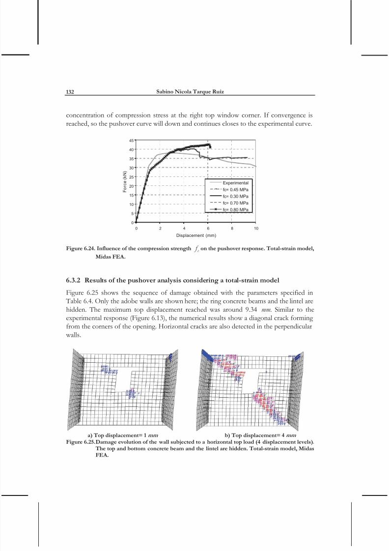
Figure 6.24 shows the numerical pushover curves obtained with different compressionstrength values. It can be observed that the best results are obtained with f c = 0.30 MPa .

The pushover curves obtained with other compression strengths are superimposed andgive higher strength, but stop earlier due to convergence problems due to the

8/12/2019 Tarque - 2011 - Chapter 6



concentration of compression stress at the right top window corner. If convergence isreached, so the pushover curve will down and continues closes to the experimental curve.

0

5

10

15

20

25

30

35

40

45

0 2 4 6 8 10

Displacement (mm)

F o r c e ( k N )

Experimental

fc= 0.45 MPa

fc= 0.30 MPa

fc= 0.70 MPa

fc= 0.80 MPa

Figure 6.24. Influence of the compression strength c f on the pushover response. Total-strain model,

Midas FEA .

6.3.2 Results of the pushover analysis considering a total-strain model

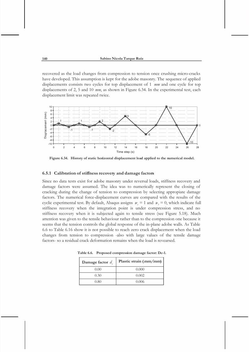
Figure 6.25 shows the sequence of damage obtained with the parameters specified in Table 6.4. Only the adobe walls are shown here; the ring concrete beams and the lintel arehidden. The maximum top displacement reached was around 9.34 mm. Similar to theexperimental response (Figure 6.13), the numerical results show a diagonal crack formingfrom the corners of the opening. Horizontal cracks are also detected in the perpendicular

walls.


Figure 6.25. Damage evolution of the wall subjected to a horizontal top load (4 displacement levels). The top and bottom concrete beam and the lintel are hidden. Total-strain model, MidasFEA.

8/12/2019 Tarque - 2011 - Chapter 6




Figure 6.24. Continuation. Damage evolution of the wall subjected to a horizontal top load (4displacement levels). The top and bottom concrete beam and the lintel are hidden. Total-strain model, Midas FEA.

Figure 6.26 shows the evolution of the maximum principal stresses on the in-plane adobe wall (the concrete beams, lintel and perpendicular walls are not shown). In the legend themaximum tensile stress value is limited to 0.05 MPa . A good agreement is seen between

the maximum tensile stresses and the experimental damage pattern (Figure 6.14). Largetensile stresses correspond to large crack openings. The principal stresses reach theirmaximum values at the opening corners and then travel to the wall corners. The whitezones inside the adobe wall show the parts where the tensile strength has been exceeded;this is possible when dealing with a fixed crack [de Borst and Nauta 1985; Feenstra andRots 2001; Noghabai 1999].

The good global agreement between the numerical results and the experimental testsleads to the conclusion that the total-strain model can be successfully applied to theanalysis of adobe masonry, and the assumption of a homogeneous material is reasonable.Figure 6.27 shows the deformation pattern at the last computation step.

The models were run in Midas FEA with arc-length method with initial stiffness. Thenumber of load steps was specified as 100, the initial load factor was 0.01, and themaximum number of iterations per load step was 800. The convergence criteria weregiven by an energy norm equal to 0.01 and a displacement norm equal to 0.005.

8/12/2019 Tarque - 2011 - Chapter 6





Figure 6.26. Evolution of maximum principal stresses in the adobe wall subjected to a horizontal topdisplacement. Total-strain model, Midas FEA.

Figure 6.27. Deformation of the adobe wall due to a maximum horizontal top displacement of 9.34mm. Total-strain model, Midas FEA.

8/12/2019 Tarque - 2011 - Chapter 6



6.4 CONCRETE DAMAGED PLASTICITY : MODELLING THE PUSHOVER RESPONSE.

A finite element model was created in Abaqus/Standard using 4-node rectangular shellelements without integration reduction (Figure 6.28a). For element controls, a finitemembrane strain and a default drilling hourglass scaling factors were selected. Thenumerical model is similar to the one created in Section 6.3 with Midas FEA, so the shellelements are 100 x 100 mm with 300 mm thick, and the characteristic length is equal to thediagonal of the shell element. The reinforced concrete beams (top and bottom) and the

wooden lintel are modelled using linear material properties. The adobe masonry isrepresented by the concrete damaged plasticity model, which takes into account the

tension and compression constitutive laws for adobe. The displacement history is appliedat one edge of the top concrete beam as seen in Figure 6.28b. The base of the foundationis fully fixed, while the top part of the crown concrete beam is free of movement.

a) Complete view of the model b) Position of horizontal applied loads at the top beam

Figure 6.28. Finite element model of the adobe wall subjected to horizontal displacement loads at thetop. Concrete Damaged Plasticity model, Abaqus/Standard.

The material parameters used in Abaqus/Standard are essentially the ones used for MidasFEA, though the compression strength is increased to 0.45 MPa as shown in Table 6.5.

Table 6.5. Material properties for the adobe masonry within concrete damaged plasticity model.

Elastic Tension Compression

E( N/mm 2 )

m

( N/mm 3 )h

( mm ) f t

( N/mm 2 )

I G

( N/mm )

f c( N/mm 2 )

c G

( N/mm )

p ( mm/mm )

200 0.2 2e-05 141.4 0.04 0.01 0.45 0.155 0.002

8/12/2019 Tarque - 2011 - Chapter 6



The following default additional parameters are required for the concrete damagedplasticity model: dilatation angle= 1, eccentricity= 0.1, ratio of initial equibiaxialcompressive yield stress to initial uniaxial compressive yield stress= 1.16, k parameterrelated to yield surface= 2/3, and null viscosity parameter.

Again, a parametric study for selection of the tensile and compression strength is carriedout. The tensile strength is between 0.02 to 006 MPa and the compression strength is

varied between 0.30 to 0.80 MPa (see Figure 6.18 and Figure 6.23). As in the previousanalysis, it is seen from the numerical pushover curves that the tensile strength is the

parameter that controls the global behaviour of the adobe masonry; low values of tensilestrength allows to a fast inelastic excursion and will end with convergence problems, high

values of tensile strength make more brittle the adobe masonry but increase its lateralstrength. According to Figure 6.29 a value of f t equal to 0.04 MPa should be selected.

0

5

10

15

20

25

30

35

40

45

50

0 2 4 6 8 10

Displacement (mm)

F o r c e ( k N )

Experimentalft= 0.02 MPa

ft= 0.04 MPa

ft= 0.06 MPa

Figure 6.29. Influence of tensile strength t f on the pushover response. Concrete damaged plasticity

model, Abaqus/Standard.

Figure 6.30 shows the numerical pushover curves analyzed with different compressionstrength values. It is seen that the compression strength increment influences on the

maximum lateral strength of the adobe wall, but it maintains similar post peak behaviourand failure pattern. The main difference in lateral strength is seen from 2 to 4 mm of topdisplacement and it is due to the biaxial interaction between tensile and compressivestrength. Less difference it is seen for the pushover curves computed with f c =0.45 MPa to 0.80 MPa .

A lower bound of f c = 0.30 MPa can be considered without loss of accuracy on the globalresponse for the plasticity damage model implemented in Abaqus. In this case, there wasa not convergence problem as seen in Midas FEA.

8/12/2019 Tarque - 2011 - Chapter 6



0

5

10

15

20

25

30

35

40

45

50

0 2 4 6 8 10

Displacement (mm)

F o r c e ( k N )

Experimental

fc= 0.30 MPa

fc= 0.45 MPa

fc= 0.70 MPa

fc= 0.80 MPa

Figure 6.30. Influence of compression strength c f on the pushover response. Concrete damaged

plasticity model, Abaqus/Standard.

For the cyclic analysis done in Section 6.5 a compression strength of 0.30 MPa is assumed

for the adobe masonry, while for the dynamic analysis performed in Section 7 the

compression strength was increased to 0.45 MPa. In both cases the relation C c G f / is

maintained as 0.344 mm .

6.4.1 Results of the pushover response considering the concrete damaged plasticity model

The displacement pattern at the last stage is shown in Figure 6.31. The global behaviourof the numerical analysis on the adobe wall represents well the experimental test in termsof crack pattern and lateral capacity (see Figure 6.14). It is preliminarily concluded thatthe calibrated material properties can be used for further numerical analyses.

Figure 6.31. Deformation of the adobe wall due to a maximum horizontal top displacement of 10mm. Concrete damaged plasticity model, Abaqus/Standard.

8/12/2019 Tarque - 2011 - Chapter 6



Furthermore, the damage pattern is analyzed based on the formation of plastic strain intension at different levels of top displacement (Figure 6.32). It is observed that theformation of cracks starts at the opening corners and at the contact zone of the lintel

with the adobe masonry. Horizontal cracks are also observed at the perpendicular walls,similarly to the ones observed in the experimental test.


c) Top displacement= 6 mm d) Top displacement= 10 mm

Figure 6.32. Evolution of maximum in-plane plastic strain in the adobe wall subjected to a horizontaltop displacement. Concrete damaged plasticity model, Abaqus/Standard.

Figure 6.33 shows the evolution of the maximum principal stresses in the in-plane adobe wall, without the two concrete beams, the timber lintel and the perpendicular walls. It is

observed that the maximum tensile zones (shown in red) are reached first at the openingcorners and evolve diagonally to the wall corners. After any integration point reaches t f ,so the tensile stress value descends but increasing the crack displacement (softening partof the tensile constitutive law).

The models were run in Abaqus/Standard specifying a direct method -for equationsolver- with full Newton solution technique. The total displacement load is applied in 1s,having a minimum increment size of 0.01 s with a maximum of 0.5 s . The maximumnumber of increments is 2000. Non linear geometric effects are considered for the

8/12/2019 Tarque - 2011 - Chapter 6



analysis of equilibrium even though they are not expected to affect the results of such astiff wall. Two control parameters are also specified, the automatic stabilization for adissipated energy fraction of 0.001, and the adaptive stabilization with maximum ratio ofstabilization to strain energy of 0.1.


c) Top displacement= 6 mm d) Top displacement= 10 mm

Figure 6.33. Evolution of maximum principal stresses in the adobe wall subjected to a horizontal topdisplacement. Concrete damaged plasticity model, Abaqus/Standard.

6.5 CONCRETE D AMAGED PLASTICITY : MODELLING THE CYCLIC BEHAVIOUR

The finite element model used for the pushover analysis in Abaqus/Standard was then

used for calibration of parameters for cyclic behaviour. The idea is to calibrate thedamage factors d t and d c (which control the closing of cracking and reduces the elasticstiffness during unloading), and the stiffness recovery t w and c w , for tension andcompression respectively, to reproduce the behaviour of adobe masonry under reversalloads. The tensile and compression strength are kept as 0.04 and 0.30 MPa , respectively.

According to Abaqus 6.9 SIMULIA [2009], it was seen from experimental tests onconcrete that the compressive stiffness can be recovered upon crack closure as the loadchanges from tension to compression. On the other hand, the tensile stiffness is not

8/12/2019 Tarque - 2011 - Chapter 6



recovered as the load changes from compression to tension once crushing micro-crackshave developed. This assumption is kept for the adobe masonry. The sequence of applieddisplacements consists two cycles for top displacement of 1 mm and one cycle for topdisplacements of 2, 5 and 10 mm , as shown in Figure 6.34. In the experimental test, eachdisplacement limit was repeated twice.

2

-2

0

1

-1

1

-1

-10

10

-5

5

-10

-8

-6

-4

-2

0

2

4

6

8

10

0 2 4 6 8 10 12 14 16 18 20 22 24 26 28

Time step (s)

D i s p

l a c e m e

n t ( m m

)

Figure 6.34. History of static horizontal displacement load applied to the numerical model.

6.5.1 Calibration of stiffness recovery and damage factors

Since no data tests exist for adobe masonry under reversal loads, stiffness recovery and

damage factors were assumed. The idea was to numerically represent the closing ofcracking during the change of tension to compression by selecting appropiate damagefactors. The numerical force-displacement curves are compared with the results of thecyclic experimental test. By default, Abaqus assigns c w = 1 and t w = 0, which indicate fullstiffness recovery when the integration point is under compression stress, and nostiffness recovery when it is subjected again to tensile stress (see Figure 5.18). Muchattention was given to the tensile behaviour rather than to the compression one because itseems that the tension controls the global response of the in-plane adobe walls. As Table6.6 to Table 6.16 show it is not possible to reach zero crack displacement when the loadchanges from tension to compression -also with large values of the tensile damagefactors- so a residual crack deformation remains when the load is revearsed.

Table 6.6. Proposed compression damage factor: Dc-1.

Damage factor c d Plastic strain (mm/mm )

0.00 0.000

0.30 0.002

0.80 0.006

8/12/2019 Tarque - 2011 - Chapter 6



Table 6.7. Proposed tensile damage factor: Dt-1.

Damage factor t d Plastic disp. (mm )

0.00 0.00

0.85 0.125

0.90 0.250

0.95 0.5000

0.005

0.01

0.015

0.02

0.025

0.03

0.035

0.04

0.045

0 0.2 0.4 0.6 0.8 1

Crack displacement (mm)

T e n s

i l e s

t r e n g

t h ( M P a

)

Tensile curve

Degradated stiffnessfor unloading



0.00 0.00

0.90 0.250

0.95 0.350

0

0.005

0.01

0.015

0.02

0.025

0.03

0.035

0.04

0.045

0 0.2 0.4 0.6 0.8 1



Tensile curve

Degradated stiffness

for unloading



0.00 0.000

0.90 0.250

0.95 0.500

0

0.005

0.01

0.015

0.02

0.025

0.03

0.035

0.04

0.045

0 0.2 0.4 0.6 0.8 1



Tensile curve


for unloading



0.00 0.000.70 0.100

0.85 0.200

0.95 0.3750

0.005

0.01

0.015

0.02

0.025

0.03

0.035

0.04

0.045

0 0.2 0.4 0.6 0.8 1


T e n s i l e s t r e n g t h ( M

P a )

Tensile curve


for unloading

8/12/2019 Tarque - 2011 - Chapter 6





0.00 0.00

0.75 0.100

0.85 0.250

0.95 0.5000

0.005

0.01

0.015

0.02

0.025

0.03

0.035

0.04

0.045

0 0.2 0.4 0.6 0.8 1


T e n s

i l e s

t r e n g

t h ( M P a

)

Tensile curve


for unloading



0.00 0.000

0.90 0.250

0

0.005

0.01

0.015

0.02

0.025

0.03

0.035

0.04

0.045

0 0.2 0.4 0.6 0.8 1


T e n s

i l e s

t r e n g

t h ( M P a

)

Tensile curve




0.00 0.00

0.80 0.100

0.90 0.200

0.95 0.3000

0.005

0.01

0.015

0.02

0.025

0.03

0.035

0.04

0.045

0 0.2 0.4 0.6 0.8 1


T e n s

i l e s

t r e n g

t h ( M P a

)

Tensile curve


for unloading


Damage factort

d Plastic disp. (mm )

0.00 0.000

0.85 0.125

0.90 0.500

0.95 0.6500

0.005

0.01

0.015

0.02

0.025

0.03

0.035

0.04

0.045

0 0.2 0.4 0.6 0.8 1


T e n s i l e s t r e n g t h ( M P a

)

Tensile curve


8/12/2019 Tarque - 2011 - Chapter 6





0.00 0.00

0.90 0.250

0.95 0.400

0

0.005

0.01

0.015

0.02

0.025

0.03

0.035

0.04

0.045

0 0.2 0.4 0.6 0.8 1



Tensile curve


for unloading



0.00 0.000

0.60 0.050

0.80 0.100

0.85 0.1500

0.005

0.01

0.015

0.02

0.025

0.03

0.035

0.04

0.045

0 0.2 0.4 0.6 0.8 1


T e n s

i l e s

t r e n g

t h ( M P a

)

Tensile curve


Figure 6.35 shows the results of the 21 models run in Abaqus under cyclic loading.

Models 1 to 4 show the effect of stiffness recovery in tension and compression withouttaking into account damage factors. The unloading branch beyond 5 mm and the loadingbranch for 10 mm do not match well the experimental curve. The numerical branchesseem to dissipate more energy that the experimental one. Models 5 to 7 show theinfluence of damage factors with variation of the stiffness recovery; these models showsome improvement matching the experimental results with respect to the previousmodels, especially the loading branch for 10 mm of displacement. However, due toconvergence problems, none of the models reached the last displacement cycle. It ispreliminarily concluded that the inclusion of damage factors allows a betterapproximation of the actual test results. The best result was obtained with c w 0.5 (Model 6). Models 8 to 12 analyze the influence of the tensile damage factor. In thesecases c w is kept at 1. It is seen that the compression stiffness recovery is needed to match

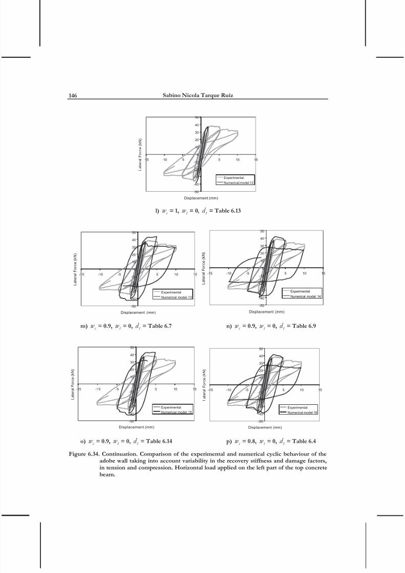
the experimental results, especially for the loading branch at 10 mm. Models 13 to 17analyze the variation of the compression recovery stiffness from 0.70 to 0.90 and thetensile damage factors. It is seen that lower values of c w should be used for a bettermatch with the experimental result in combination with the tensile damage parameterfrom Table 6.7 or Table 6.8. The unloading branch after the 5 mm displacement stillshows large residual deformations for a lateral load equal to 0 kN , which is not inagreement with the experimental observations. It is understood that this phenomenadepends basically on the tensile damage factors applied to the masonry; however, specialattention should be paid to the selection of t d values in order to avoid convergence

8/12/2019 Tarque - 2011 - Chapter 6



problems. Models 18 to 21 maintain the tensile damage factor specified in Table 6.7, which are close to the ones specified in Table 6.9, but with a variation of the compressionstiffness recovery from 0.5 to 0.8. The best match is obtained with Model 20, whichconsidered c w 0.6 , despite the large residual deformations.

-50

-40

-30

-20

-10

0

10

20

30

40

50

-15 -10 -5 0 5 10 15

Displacement (mm)

L a t e r a l F

o r c e ( k N )

Experimental

Numerical model 1

-50

-40

-30

-20

-10

0

10

20

30

40

50

-15 -10 -5 0 5 10 15

Displacement (mm)

L a

t e r a l

F o r c e

( k N )

Experimental

Numerical model 2

a) c w = 1, t w = 0, no damage factor b) c w = 1, t w = 0.9, no damage factor

-50

-40

-30

-20

-10

0

10

20

30

40

50

-15 -10 -5 0 5 10 15

Displacement (mm)

L a

t e r a

l F o r c e

( k N )

Experimental

Numerical model 3

-50

-40

-30

-20

-10

0

10

20

30

40

50

-15 -10 -5 0 5 10 15

Displacement (mm)

L a t e r a l F o r c e ( k N )

Experimental

Numerical model 4

c) c w = 0.75, t w = 0, no damage factor d) c w = 0.5, t w = 0, no damage factor

-50

-40

-30

-20

-10

0

10

20

30

40

-15 -10 -5 0 5 10 15

Displacement (mm)

L a t e r a l F o r c

e ( k N )

Experimental

Numerical model 5

-40

-30

-20

-10

0

10

20

30

40

50

-15 -10 -5 0 5 10 15

Displacement (mm)


Experimental

Numerical model 6

e) c w = 1, t w = 0, c d =Table 6.6, t d =Table 6.7 f) c w = 0.5, t w = 0.5, c d =Table 6.6, t d =Table 6.8

8/12/2019 Tarque - 2011 - Chapter 6



-40

-30

-20

-10

0

10

20

30

40

50

-15 -10 -5 0 5 10 15

Displacement (mm)


Experimental

Numerical model 7

g) c w = 0.5, t w = 0.5, c d = Table 6.6, t d = Table 6.9

-40

-30

-20

-10

0

10

20

30

40

50

-15 -10 -5 0 5 10 15

Displacement (mm)


Experimental

Numerical model 8

-50

-40

-30

-20

-10

0

10

20

30

40

50

-15 -10 -5 0 5 10 15

Displacement (mm)


Experimental

Numerical model 9

h) c w = 1, t w = 0, t d = Table 6.7 i) c w = 1, t w = 0, t d = Table 6.10

-50

-40

-30

-20

-10

0

10

20

30

40

50

-15 -10 -5 0 5 10 15

Displacement (mm)


Experimental

Numerical model 10

-50

-40

-30

-20

-10

0

10

20

30

40

50

-15 -10 -5 0 5 10 15

Displacement (mm)


Experimental

Numerical model 11

j) c w = 1, t w = 0, t d = Table 6.11 k) c w = 1, t w = 0, t d = Table 6.12

Figure 6.35. Comparison of the experimental and numerical cyclic behaviour of the adobe wall takinginto account variability in the recovery stiffness and damage factors, in tension andcompression. Horizontal load applied on the left part of the top concrete beam.

8/12/2019 Tarque - 2011 - Chapter 6



-50

-40

-30

-20

-10

0

10

20

30

40

50

-15 -10 -5 0 5 10 15

Displacement (mm)


Experimental

Numerical model 12

l) c w = 1, t w = 0, t d = Table 6.13

-50

-40

-30

-20

-10

0

10

20

30

40

50

-15 -10 -5 0 5 10 15

Displacement (mm)


Experimental

Numerical model 13

-50

-40

-30

-20

-10

0

10

20

30

40

50

-15 -10 -5 0 5 10 15

Displacement (mm)


Experimental

Numerical model 14

m) c w = 0.9, t w = 0, t d = Table 6.7 n) c w = 0.9, t w = 0, t d = Table 6.9

-50

-40

-30

-20

-10

0

10

20

30

40

50

-15 -10 -5 0 5 10 15

Displacement (mm)

L a

t e r a

l F o r c e

( k N )

Experimental

Numerical model 15

-50

-40

-30

-20

-10

0

10

20

30

40

50

-15 -10 -5 0 5 10 15

Displacement (mm)


Experimental

Numerical model 16

o) c w = 0.9, t w = 0, t d = Table 6.14 p) c w = 0.8, t w = 0, t d = Table 6.4

Figure 6.34. Continuation. Comparison of the experimental and numerical cyclic behaviour of theadobe wall taking into account variability in the recovery stiffness and damage factors,in tension and compression. Horizontal load applied on the left part of the top concretebeam.

8/12/2019 Tarque - 2011 - Chapter 6



-50

-40

-30

-20

-10

0

10

20

30

40

50

-15 -10 -5 0 5 10 15

Displacement (mm)


Experimental

Numerical model 17

q) c w = 0.7, t w = 0, t d = Table 6.8

-40

-30

-20

-10

0

10

20

30

40

50

-15 -10 -5 0 5 10 15

Displacement (mm)


Experimental

Numerical model 18

-40

-30

-20

-10

0

10

20

30

40

50

-15 -10 -5 0 5 10 15

Displacement (mm)


Experimental

Numerical model 19

r) c w = 0.8, t w = 0, t d = Table 6.7 s) c w = 0.7, t w = 0, t d = Table 6.7

-50

-40

-30

-20

-10

0

10

20

30

40

50

-15 -10 -5 0 5 10 15

Displacement (mm)


Experimental

Numerical model 20

-50

-40

-30

-20

-10

0

10

20

30

40

50

-15 -10 -5 0 5 10 15

Displacement (mm)

L a e r a l F o r c e ( k N )

Experimental

Numerical model 21

t) c w = 0.6, t w = 0, t d = Table 6.7 u) c w = 0.5, t w = 0, t d = Table 6.7

Figure 6.34. Continuation. Comparison of the experimental and numerical cyclic behaviour of theadobe wall taking into account variability in the recovery stiffness and damage factors,in tension and compression. Horizontal load applied on the left part of the top concretebeam.

8/12/2019 Tarque - 2011 - Chapter 6



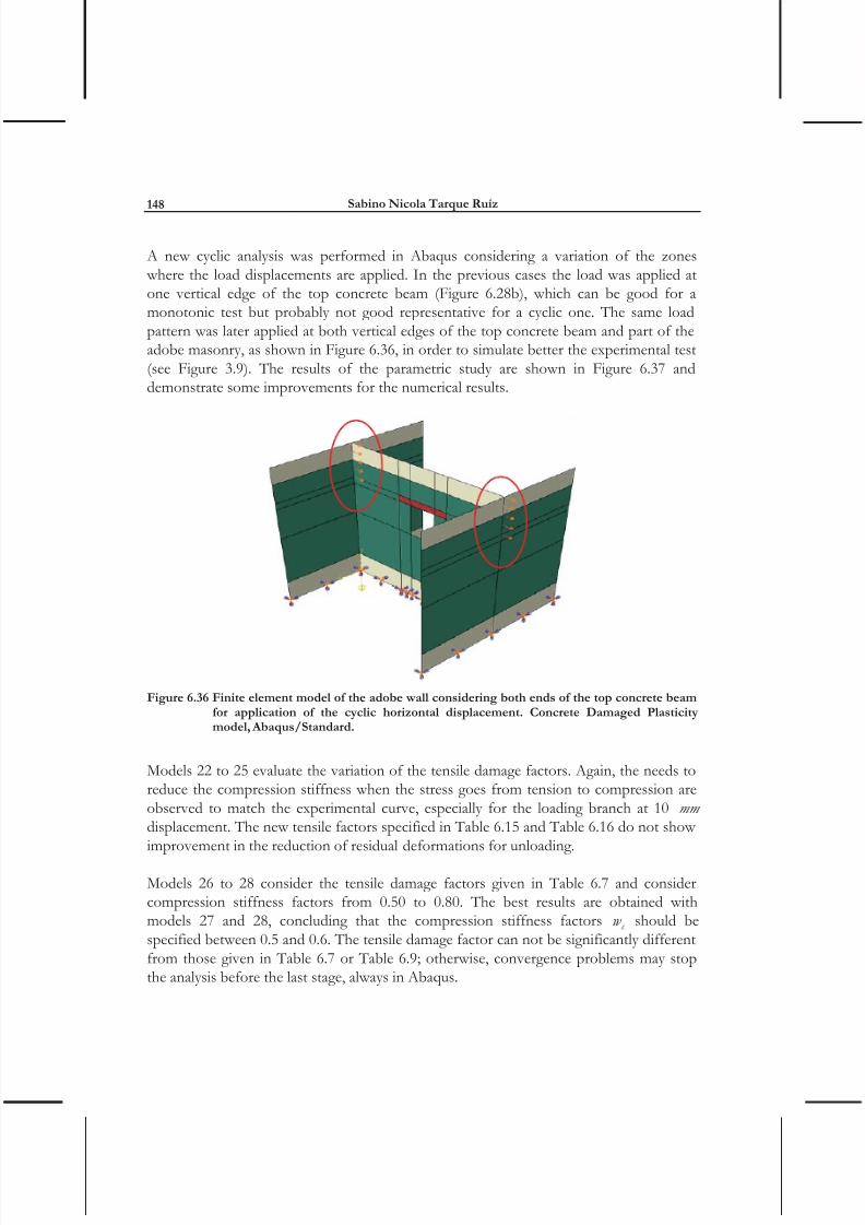
A new cyclic analysis was performed in Abaqus considering a variation of the zones where the load displacements are applied. In the previous cases the load was applied atone vertical edge of the top concrete beam (Figure 6.28b), which can be good for amonotonic test but probably not good representative for a cyclic one. The same loadpattern was later applied at both vertical edges of the top concrete beam and part of theadobe masonry, as shown in Figure 6.36, in order to simulate better the experimental test(see Figure 3.9). The results of the parametric study are shown in Figure 6.37 anddemonstrate some improvements for the numerical results.

Figure 6.36 Finite element model of the adobe wall considering both ends of the top concrete beamfor application of the cyclic horizontal displacement. Concrete Damaged Plasticitymodel, Abaqus/Standard.

Models 22 to 25 evaluate the variation of the tensile damage factors. Again, the needs toreduce the compression stiffness when the stress goes from tension to compression areobserved to match the experimental curve, especially for the loading branch at 10 mm displacement. The new tensile factors specified in Table 6.15 and Table 6.16 do not showimprovement in the reduction of residual deformations for unloading.

Models 26 to 28 consider the tensile damage factors given in Table 6.7 and considercompression stiffness factors from 0.50 to 0.80. The best results are obtained withmodels 27 and 28, concluding that the compression stiffness factors c w should bespecified between 0.5 and 0.6. The tensile damage factor can not be significantly differentfrom those given in Table 6.7 or Table 6.9; otherwise, convergence problems may stopthe analysis before the last stage, always in Abaqus.

8/12/2019 Tarque - 2011 - Chapter 6



-50

-40

-30

-20

-10

0

10

20

30

40

50

-15 -10 -5 0 5 10 15

Displacement (mm)


Experimental

Numerical model 22

-50

-40

-30

-20

-10

0

10

20

30

40

50

-15 -10 -5 0 5 10 15

Displacement (mm)

a e r a

o r c e

Experimental

Numerical model 23

a) c w = 1, t w = 0, t d = Table 6.7 b) c w = 1, t w = 0, t d = Table 6.9

-50

-40

-30

-20

-10

0

10

20

30

40

50

-15 -10 -5 0 5 10 15

Displacement (mm)


Experimental

Numerical model 24

-50

-40

-30

-20

-10

0

10

20

30

40

50

-15 -10 -5 0 5 10 15

Displacement (mm)


Experimental

Numerical model 25

c) c w = 1, t w = 0, t d = Table 6.15 d) c w = 1, t w = 0, t d = Table 6.16

-50

-40

-30

-20

-10

0

10

20

30

40

50

-15 -10 -5 0 5 10 15

Displacement (mm)


ExperimentalNumerical model 26

-50

-40

-30

-20

-10

0

10

20

30

40

50

-15 -10 -5 0 5 10 15

Displacement (mm)


ExperimentalNumerical model 27

e) c w = 0.8, t w = 0, t d = Table 6.7 f) c w = 0.6, t w = 0, t d = Table 6.7

Figure 6.37. Comparison of the experimental and numerical cyclic behaviour of the adobe wall takinginto account variability in the recovery stiffness and damage factors, in tension andcompression. Horizontal load applied at both ends of the top concrete beam.

8/12/2019 Tarque - 2011 - Chapter 6



-50

-40

-30

-20

-10

0

10

20

30

40

50

-15 -10 -5 0 5 10 15

Displacement (mm)


Experimental

Numerical model 28

g) c w = 0.5, t w = 0, t d = Table 6.7

Figure 6.37. Continuation. Comparison of the experimental and numerical cyclic behaviour of theadobe wall taking into account variability in the recovery stiffness and damage factors.Horizontal load applied at both ends of the top concrete beam.

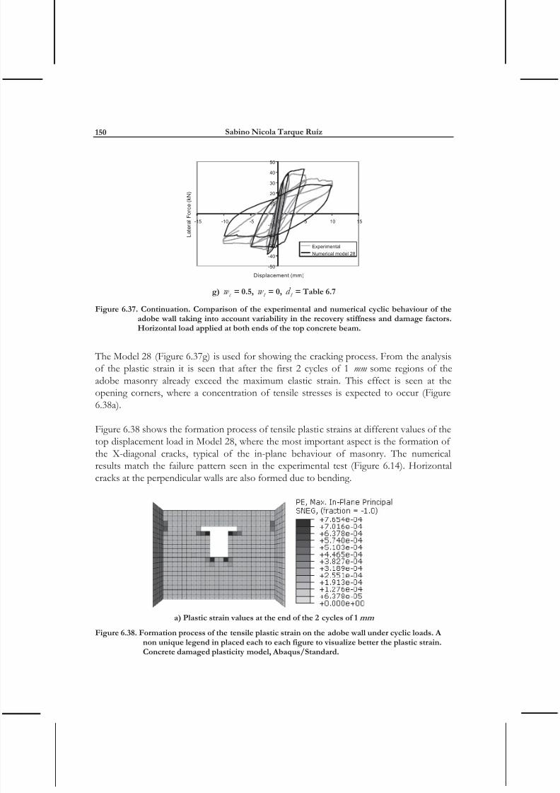
The Model 28 (Figure 6.37g) is used for showing the cracking process. From the analysisof the plastic strain it is seen that after the first 2 cycles of 1 mm some regions of theadobe masonry already exceed the maximum elastic strain. This effect is seen at theopening corners, where a concentration of tensile stresses is expected to occur (Figure6.38a).

Figure 6.38 shows the formation process of tensile plastic strains at different values of thetop displacement load in Model 28, where the most important aspect is the formation ofthe X-diagonal cracks, typical of the in-plane behaviour of masonry. The numericalresults match the failure pattern seen in the experimental test (Figure 6.14). Horizontalcracks at the perpendicular walls are also formed due to bending.

a) Plastic strain values at the end of the 2 cycles of 1 mm

Figure 6.38. Formation process of the tensile plastic strain on the adobe wall under cyclic loads. Anon unique legend in placed each to each figure to visualize better the plastic strain.Concrete damaged plasticity model, Abaqus/Standard.

8/12/2019 Tarque - 2011 - Chapter 6



c) Plastic strain values at the end of the cycle of 5 mm

d) Plastic strain values at the end of the cycle of 10 mm

Figure 6.38. Continuation. Formation process of the tensile plastic strain on the adobe wall undercyclic loads. A non unique legend in placed each to each figure to visualize better the plastic strain. Concrete damaged plasticity model, Abaqus/Standard.

Another way for interpretation of the tensile damage occurred in the adobe masonry is toshow the tensile damage factor (Figure 6.39).

Figure 6.39. Tensile damage factor for Model 28 at the end of the history of cyclic horizontaldisplacement load.

8/12/2019 Tarque - 2011 - Chapter 6



The tensile damage factor is a non-decreasing quantity associated with the tensile failureof the material. In Figure 6.39, the zones which are not in blue ( t d = 0) indicate the zones

which already are in the softening part of the tensile constitutive law and can beinterpreted as damage zones.

6.6 V IBRATION MODES

An eigenvalue analysis is done to compute the vibration modes of the model, especially inthe direction of the applied load (X-X direction). The reinforced concrete beam placed as

foundation of the wall is removed, so the total weight of the model is 100.63 kN . Thebase of the wall is fully fixed. The analysis is performed with Abaqus/Standard throughthe linear perturbation option and considering Lanczos method for extraction of thefrequency values. A 50% of the elasticity of modulus has been used according to Tarque[2008] to take into account early cracking into the material. Figure 6.40 shows theeffective mass related to the first 11 vibration modes, represented here by the frequency

values. In theory the sum of all the effective masses should be equal to the total mass ofthe model. It is seen that 11 modes of vibration are required to reach the 90% of the totalmass (Table 6.17), being the fundamental one the first mode.

0

10

20

30

40

50

60

70

80

8.644 18.753 25.583 29.053 36.399 41.283 45.337 53.734 55.388 58.641 61.147

Frequency (Hz)

E f f e c

t i v e m a s s

( % )

Figure 6.40. Contribution of the modes of vibration in the X-X direction until reaches the 90% of the

total mass of the model.

The deflected shapes given for each mode of vibration are shown in Figure 6.41. The first vibration mode, which involves 74.24% of the total mass, is a translational mode; whilethe others are basically out-of-plane deformations of the flange walls. This analysisconsiders the use of the elastic material properties. However, the adobe material is brittleand goes into the inelastic range very early; therefore the frequencies are expected toshorten.

8/12/2019 Tarque - 2011 - Chapter 6



a) Mode 1. T1= 0.1157s b) Mode 2. T2= 0.0533s

c) Mode 3. T3= 0.0391s d) Mode 4. T4= 0.0344s

e) Mode 5. T5= 0.0275s f) Mode 6. T6= 0.0242s

Figure 6.41. Modes of vibration in the X-X direction.

8/12/2019 Tarque - 2011 - Chapter 6



Table 6.17. Values of the frequency and period of vibrations of the numerical model in the X-Xdirection.

Mode number % effective mass (%) Frequency (Hz) Period (s)

1 74.2347 74.235 8.64 0.1157

2 1.1936 75.428 18.75 0.0533

3 1.5037 76.932 25.58 0.0391

4 5.5291 82.461 29.05 0.0344

5 2.2419 84.703 36.40 0.02756 1.7464 86.449 41.28 0.0242

7 0.8635 87.313 45.34 0.0221

8 0.2657 87.579 53.73 0.0186

9 1.4834 89.062 55.39 0.0181

10 0.0286 89.091 58.64 0.0171

11 1.3749 90.466 61.15 0.0164

6.7 ENERGY BALANCE FOR QUASI-STATIC ANALYSIS

The energy balance of the entire model should be checked to ensure that the timeincrement is not causing instability and the solution of the model is correct. Theconservation of energy implies that the total energy Etotal should be constant and close tozero. The total energy is given by:

total KE IE VD SD KL JD W E E E E E E E E (6.9)

where EKE is the kinetic energy, EIE is the total internal energy, EVD is the visco-elasticenergy, ESD is the static energy due to stabilization, EKL is the loss of kinetic energy atimpact, E JD is the electrical energy dissipated due to flow of electrical current, and EW isthe work done by the externally applied loads. For this quasi static problem the EKE, EVD ,

EKL and E JD are zero energy.

The total internal energy is given by:

I SE PD CD AE QB EE DMD E E E E E E E E (6.10)

where ESE is the recoverable strain energy, EPD is the energy due to plastic dissipation, ECD is the energy dissipated by creep, E AE is the artificial energy, E QB is the energydissipated through quiet boundaries, E EE is the electrostatic energy, and EDMD is the

8/12/2019 Tarque - 2011 - Chapter 6



energy dissipated by damage. For the analysis made here the ECD , E QB, E EE are zeroenergy.

Figure 6.42a shows the components of the total internal energy. It is seen that after 10 s the plastic energy becomes important, which correspond to the cycles of 2 mm topdisplacement. Figure 6.42b shows the components of the total energy. Here it is seen thatthe static energy for stabilization has almost no influence on the total response, which isan indication of proper finite element solution. The energy values are plotted until 29 s because it is the total time necessary to apply the full cyclic load.

0 . E + 0 0

2 . E + 0 5

4 . E + 0 5

6 . E + 0 5

8 . E + 0 5

1 . E + 0 6

0 5 10 15 20 25 30

Time (s)

W h o l e m o d e l e n e r g y ( N - m m )

Internal work

Plastic dissipated energy

Elastic strain energy

Artificial strain energy

Damage dissipated energy

0 . E + 0 0

2 . E + 0 5

4 . E + 0 5

6 . E + 0 5

8 . E + 0 5

1 . E + 0 6

0 5 10 15 20 25 30

Time (s)

W h o l e m o d e l e n e r g y ( N - m m )

External work

Internal work

Static dissipated energy (stabilization)

a) Total internal energy b) Total energy in the model

Figure 6.42. Energy balance for Model 28, non-linear static analysis with concrete damaged plasticitymodel in Abaqus/Standard. .

6.8 SUMMARY

Two finite element approaches were used for modelling the in-plane response of anadobe wall: the discrete and the continuum approach. For the first, the combinedcracking-shearing-crushing interface model developed in Midas FEA was used. In thiscase the adobe bricks are modelled with elastic properties and the inelasticity of the adobematerial is concentrated at the mud mortar interfaces. For the second one, two models

were used: the total-strain model and the concrete damaged plasticity model.

The total-strain model is used in Midas FEA, while the concrete damaged plasticity isused in Abaqus/Standard and Abaqus/Explicit. At the beginning, only a monotonicpushover displacement was considered on the adobe walls for calibration of the adobematerial properties in Midas FEA and Abaqus/Standard. Special care was paid to theinelastic properties. When the numerical failure pattern and the numerical force-displacement curve matched the experimental one in a satisfactory way, another study

8/12/2019 Tarque - 2011 - Chapter 6



was done in Abaqus/Standard to simulate the cyclic response on an adobe wall. This way,damage factors and stiffness recovery in tension and compression were calibrated in viewof the complete seismic analysis of adobe walls (see Chapter 7). The cyclic response wasnot able to be reproduced in Midas FEA due to difficulties in convergence for reversalloads.

Tarque - 2011 - Chapter 6

Documents

Transcript of Tarque - 2011 - Chapter 6