TAPP, ANNA F., M.A. Mapping the Impact of Vegetation and Terrain on Cellular Signal

Levels. (2008)

Directed by Dr. Rick L. Bunch. 60pp

The purpose of this research is to look into the impact that rough topography

combined with dense vegetation can have on a digital cellular phone signal. The research

area is the Deep Creek region of the Great Smoky Mountains National Park. In addition

to hosting an unmatched amount of biological diversity for its acreage, the Great Smoky

Mountains National Park is the most visited U.S. national park.

A classified vegetation map of the park was obtained from the National Park

Service. An all returns LIDAR dataset was used to create a terrain model and a tree

canopy model. Field measurements were conducted in both leaf on and leaf off

conditions along the trails of the Deep Creek region, located north of Bryson City and

south of Clingman’s Dome.

Significant relationships were found relating soil moisture and tree heights to

attenuation. Soil moisture was found to have a significant impact on the leaf on v. leaf

off difference. The height of the tree canopy was a more significant contributor to

attenuation than the species of the tree. In this study the species of tree was only

significant insomuch as it was an indicator of the tree height.

MAPPING THE IMPACT OF VEGETATION AND

TERRAIN ON CELLULAR SIGNAL LEVELS

by

Anna F. Tapp

A Thesis Submitted to

the Faculty of The Graduate School at

The University of North Carolina at Greensboro

in Partial Fulfillment

of the Requirements for the Degree

Master of Arts

Greensboro

2008

Approved by

____________________________________

Rick L. Bunch, PhD, Committee Chair

ii

APPROVAL PAGE

This thesis has been approved by the following committee of the Faculty of The

Graduate School at The University of North Carolina at Greensboro.

Committee Chair ________________________________________

Rick L. Bunch, PhD

Committee Members _________________________________________

Roy S. Stine, PhD

_

______________ ________________________________________

Robert Y. Li, PhD

April 11, 2008 _

Date of Acceptance by Committee

April 4, 2008 _

Date of Final Oral Examination

iii

ACKNOWLEDGEMENTS

Thanks to Dr. Rick Bunch for his perpetual assistance and expertise. Thanks to

CityScape Consultants, Inc. for their technical guidance. A special thanks to Stephanie

Jane Edwards, Kirsten Hunt and Kay Miles for their hours of hiking through the woods.

Finally, none of this would have been possible without the help of Andrew Tapp, my

support team and permanent field partner. The field work was funded by the Center for

Geographic Information Science and Health at the University of North Carolina at

Greensboro.

iv

TABLE OF CONTENTS

Page

LIST OF TABLES .............................................................................................................. v

LIST OF FIGURES............................................................................................................ vi

CHAPTER

VII. INTRODUCTION.................................................................................................. 1

VII. CELLULAR PHONE COVERAGE MODELING................................................ 4

.III. TERRAIN AND CANOPY MODELING.............................................................. 9

Line of Sight Calculations ........................................................................... 9

Tree Canopy Model ................................................................................... 13

Diffraction Estimates................................................................................. 14

IIV. AVAILABLE DATA ........................................................................................... 17

Cell Phone Tower Data Set ....................................................................... 17

LIDAR Data Set......................................................................................... 19

Vegetation Classification Data Set ........................................................... 19

IIV. METHODOLOGY ............................................................................................... 21

Field Data Collection................................................................................ 21

Elevation Model Creation ......................................................................... 23

Predicted Signal Strength Calculations .................................................... 25

IVI. ANALYSIS AND RESULTS .............................................................................. 28

Accuracy Assessments ............................................................................... 28

Statistical Analysis .................................................................................... 36

VII. CONCLUSION .................................................................................................... 45

REFERENCES.................................................................................................................. 48

v

LIST OF TABLES

Page

Table 5.1. Measurements for Reference Power Calculation............................................ 26

Table 5.2. Reference Power Values ................................................................................. 26

Table 6.1. Consolidation of Analysis Categories............................................................. 35

Table 6.2. Distribution of Sample by Vegetation Analysis Class.................................... 35

Table 6.3. ANOVA Test Results With Signal Strength as the Dependent Variable........ 37

Table 6.4. ANOVA Test Results With Tree Canopy Height and Distance from

Dominant Antenna as the Dependent Variables ........................................ 39

Table 6.5. Correlation Test Results With Signal Strength as the Dependent Variable.... 41

vi

LIST OF FIGURES

Page

Figure 2.1. Ideal Cellular Network..................................................................................... 4

Figure 3.1. Viewshed Classification .................................................................................. 9

Figure 3.2. Multiple Knife-Edge Diffraction ................................................................... 14

Figure 4.1. Three Sector Antenna Propagation Pattern.................................................... 17

Figure 4.2. Geographic Research Area ............................................................................ 18

Figure 5.1. Field Data Collection Locations .................................................................... 22

Figure 5.2. Sample Profile Between Transmitter and Receiver ....................................... 26

Figure 6.1. Histogram of Elevation Errors....................................................................... 29

Figure 6.2. Histogram of Canopy Height Errors.............................................................. 30

Figure 6.3. Line of Sight Signal Strength Readings Compared to Free Space Model..... 31

Figure 6.4. Ideal Free Space Plus Diffraction Model Compared to Observed Values .... 32

Figure 6.5. Ideal Free Space Plus Diffraction Model Error, Leaf On and Leaf Off ........ 33

Figure 6.6. Soil Moisture as the Main Effect for the Difference Between Leaf Off

and Leaf On Measurements....................................................................... 37

Figure 6.7. Vegetation Class as the Main Effect for the Difference Between Leaf

Off and Leaf On Measurements ................................................................ 38

Figure 6.8. Four Vegetation Classes as the Main Effect for the Measured Canopy

Height ....................................................................................................... 39

Figure 6.9. Soil Moisture as the Main Effect for the Measured Canopy Height ............. 40

Figure 6.10. Vegetation Class as the Main Effect for the Difference Between Leaf

On and Leaf Off Measurements .............................................................. 42

1

CHAPTER I

INTRODUCTION

Over the last decade the world has experienced an explosion in cellular phone

technology and innovation. In 1995, the number of cellular phones in the United States

was 28 million. In 2001, the estimate was 118 million. In 2007 the numbers rose to 243

million subscribers (CTIA 2007). With this growing popularity, a demand has developed

for access to information and communication at all times. Some view their cellular

phones purely as recreational tools, while many others take comfort in the possession of

mobile technology as a safeguard. Even the individual who does not regularly use a

mobile phone may carry it with them “just in case.” The assumption is that the

technology will be fully functional when the user has a need. With over 210,000 cell

phone tower sites in the country, that assumption is often a reality (CTIA 2007).

Whether for convenience or for emergency, the interest is greater now than ever before to

accurately predict when and where one can make a call. Engineers are collaborating with

geographers to develop these prediction models quickly and accurately.

As individuals became increasingly dependent on mobile technology, the Federal

Communications Commission (FCC) was forced to keep pace with innovation. In 1996

the FCC recognized the growing popularity of cellular communications when it passed

rules establishing Enhanced 911 (E911). E911 was divided into two phases. In the first

phase, wireless providers were required to report the phone number of callers dialing 911

2

along with the location of the antenna that handled the call. In the second phase, wireless

providers were required to have the ability to transmit the location of a caller with an

accuracy of fifty to three hundred meters (FCC 2000). Wireless providers had until

September of 2003 to completely satisfy both phases of E911 (FCC 2005). Five years

later, with positioning technology now firmly embedded in the cellular world, cell phone

users have begun to take E911 for granted.

In the last several years, research has flooded the communications engineering

world related to signal transmission in urban environments. Meanwhile stories continue

to be published in the media related to rural accidents in which there was no cellular

tower in range. USA Today wrote that in August 2007 alone, four separate hiking

incidents made headlines (Copeland 2007). In one incident, hikers in New Jersey were

able to use a cell phone to get help from the police. Others were not so lucky. In Oregon

two hikers had to remain trapped for days in the wilderness before being reported missing

by a concerned employer. Even the best wireless positioning technology is of no use

unless there is an antenna to receive both the location signal and the call for help.

Therefore the need to accurately predict radio frequency transmission is important not

only in the urban environment, but also in the rural context.

The problem of weak cellular coverage in parks is a sensitive issue for many

nature-lovers. As much as hikers would enjoy the security of cell phone coverage on

their journeys, the existence of cell phone towers inside a preserved park impairs the

natural landscape. Therefore if towers are to be placed inside or close to preserved parks,

their numbers would have to be minimized and their appearances camouflaged as much

3

as possible. In order for the number of towers to be minimized, a volume of research is

important to predicting the behavior of the signal in a densely forested environment.

The purpose of this research is to look into the impact that rough topography

combined with dense vegetation can have on a digital cellular phone signal. The

hypothesis is that radio signal field measurements in densely vegetated areas will be

weaker than predicted values. If the hypothesis is confirmed, the subsequent goal is to

determine how different environmental variables impact signal loss to different degrees.

The research area is the Deep Creek region of the Great Smoky Mountains National Park.

In addition to hosting an unmatched amount of biological diversity for its acreage, the

Great Smoky Mountains National Park is the most visited U.S. national park, with eight

to ten million visitors each year (NPS 2007). The National Park Service credits its

popularity to its central location on the East Coast as well as its situation at the end of the

Blue Ridge Parkway. Approximately one hundred and twenty-nine incidents occur in the

park annually (NPS 2007), including at least one accidental fatality (Fraser 2002).

Five sets of data are vital in the consideration of this research problem:

- Cell phone tower sites,

- Terrain elevation grid,

- Vegetation height grid,

- Vegetation classification data,

- And a baseline pathloss prediction.

Each data set adds a vital layer to the analysis of radio frequency signal loss.

4

CHAPTER II

CELLULAR PHONE COVERAGE MODELING

Cellular phone technology is based on the concept of dividing the landscape into

coverage cells typically three miles in diameter. Each cell can handle from five to fifty

calls simultaneously (Molish 2005). Each provider is granted a limited amount of

bandwidth by the FCC. By dividing and sub-dividing the landscape into cells, wireless

providers are able to continuously increase capacity while maintaining the same small

amount of bandwidth. Since each tower only transmits across a limited distance,

frequencies can be reused by non-adjacent cells without causing destructive interference.

The network is purposely designed so that each cell overlaps in part with multiple

others (see Figure 2.1). The overlapping sections are referred to as “handoff zones”. If

Figure 2.1. Ideal Cellular Network

5

the user is in motion and passes through a handoff zone, one tower will take over for the

next in a seamless transition. The user can be traveling as fast as 150 km/hr (92.5 mi/hr)

and never know he or she is being handed from one tower to another (Molish 2005).

When determining the range and effectiveness of a cellular antenna, researchers

calculate the path loss (also called attenuation) of the wave as it travels through space.

Calculations are made using either milliwatts or decibels with respect to milliwatts

(dBm). Results are often reported in dBm’s, a convenient logarithmic unit. Free space

loss is the amount of fading a radio wave will experience in a perfect, clutter-free

environment (Rappaport 2002). Shown in Equation 2.1, free space loss can be derived

mathematically.

Friis Free Space Equation ( ) Ld

GGPd rtr

22

2

4)Pr(

π

λ=

Pr(d) = received power (mW) as a function of distance

d = distance in m

Pt = transmitter power (mW)

Gt = transmitter gain (unitless)

Gr = receiver gain (unitless)

L = system loss factor

Since such a perfect environment does not exist in experience, practical formulas used to

predict path loss in the real world are empirical in nature. Each formula has been derived

and refined through repeated field tests. The results of field tests are plotted and a fitted

curve generated. The equation of the curve is published along with the appropriate

frequency range and environmental situation under which it can be reliably applied.

Empirical equations have been generated and refined to reflect the amount of loss that

(2.1)

6

will be generally experienced in urban and suburban environments at various frequencies

(Hata 1980; Walfisch and Bertoni 1988).

L = 46.3 + 33.9 log f – 13.82 log hB +

[44.9 – 6.55 log hB] log d – CH + C

CH = 3.2 [log (11.75 hB )]2 – 4.97

L = path loss in dbm

f = frequency in MHz

d = distance in km

hB = antenna (base station) height

C = 0 db for medium and suburban, 3 db for for urban

Where f is between 1500 and 2000 MHz, receiver height is up to 10m, base station antenna height is 30 to 100m

and distance between receiver and antenna is up to 20km, and ground clutter is open, urban or suburban.

Equations 2.2.1 and 2.2.2 are the COST-231 formula, which is applicable in urban and

suburban areas with frequencies between 1500 and 2000 MHz (Walfisch and Bertoni

1988).

The major drawback to this type of model is the assumption that the ground cover

across one’s entire area can be classified uniformly. In the example of the COST-231

model, C (known as the clutter value) is a constant. When used in application, the

COST-231 suggests one of two C values for urban or suburban.

GIS has the capacity for making this type of calculation more robust with the

entrance of land cover classes. Publicly available land cover datasets can be used to

differentially calculate the path loss across the coverage map. Within the same map areas

classified as urban can be calculated differently than areas classified as suburban.

The incorporation of geospatial datasets has produced an impetus to move beyond

these average empirical formulas to more precise propagation calculations. Researchers

(2.2.1)

(2.2.2)

7

are increasingly interested in quantifying to what extent more specific forms of ground

clutter interfere with the signal. For example, how does a wooden structure interfere with

the signal compared to a concrete structure? Given this kind of information, the “urban”

class can be broken down into innumerable sub-categories, each with its own clutter

value. As technology and research progresses, the goal is to create a model that begins

with a free space calculation and from there adds each known variable, from weather to

building materials to vegetation types, to produce increasingly accurate path loss

predictions.

Rubinstein took a step in this direction in his 1998 research. He overlaid Land

Use Land Cover (LULC) data over his measurement points. He calculated the difference

between measured and predicted values for three separate band-widths. The differences

within each LULC class were averaged to arrive at an estimated clutter value for each

class located within the research area. Although this study takes a strong step by using

national geospatial data to predict signal strength, the choice of using the LULC dataset

for this application was slightly problematic. A radio wave is impacted most by the

physical nature of the land cover and not by the way the land is being used. For example,

LULC distinguishes between a lake or reservoir, and industrial or commercial. The

behavior of a radio signal will be no different based solely on the cultural usage of a body

of water or building. There can also be wide land cover variations within land use

categories that could throw off the results, especially in urban and suburban applications.

Existing research has primarily focused on urban and suburban areas, where most

of the cellular customers reside. A smaller body of research has attempted to pinpoint the

8

impact of vegetation on wave attenuation. These studies unanimously agree that

vegetation has a strong impact on the fading of a radio wave (Vogel and Goldhirsh 1986;

Tewari, et al. 1990; Goldman and Swenson 1999; Dal Bello, et al. 2000). Unlike

research conducted in urban environments, there have been limited attempts to quantify

the impact of various forms of vegetation.

One such attempt was made in 2002, at the behest of the United Kingdom

Radiocommunications Agency. The company QinetiQ attempted to create a generic

model of propagation through vegetation. In their research, they used five specific types

of trees as benchmarks – sycamore, silver maple, London plane, horse chestnut and

common lime. The excess loss as a wave passes through these types of trees (or trees

with similar leaf sizes and leaf area indices) can be calculated under this paradigm.

Unfortunately its application is limited to environments with similar tree types and no

undercanopy. Additionally, this study made no attempt to measure differences between

leaf on and leaf off situations.

The door is open for further investigation into the impact of vegetation on the

fading of radio waves. Past research has been limited to one or few vegetation types per

study. The National Park Service has completed a massive vegetation classification

project for the Great Smoky Mountains. The dataset divides this region into forty classes

of over and undercanopy. This detailed classification scheme combined with the

vegetative diversity of the area makes it an ideal location for research focusing on

vegetation native to the United States.

9

CHAPTER III

TERRAIN AND CANOPY MODELING

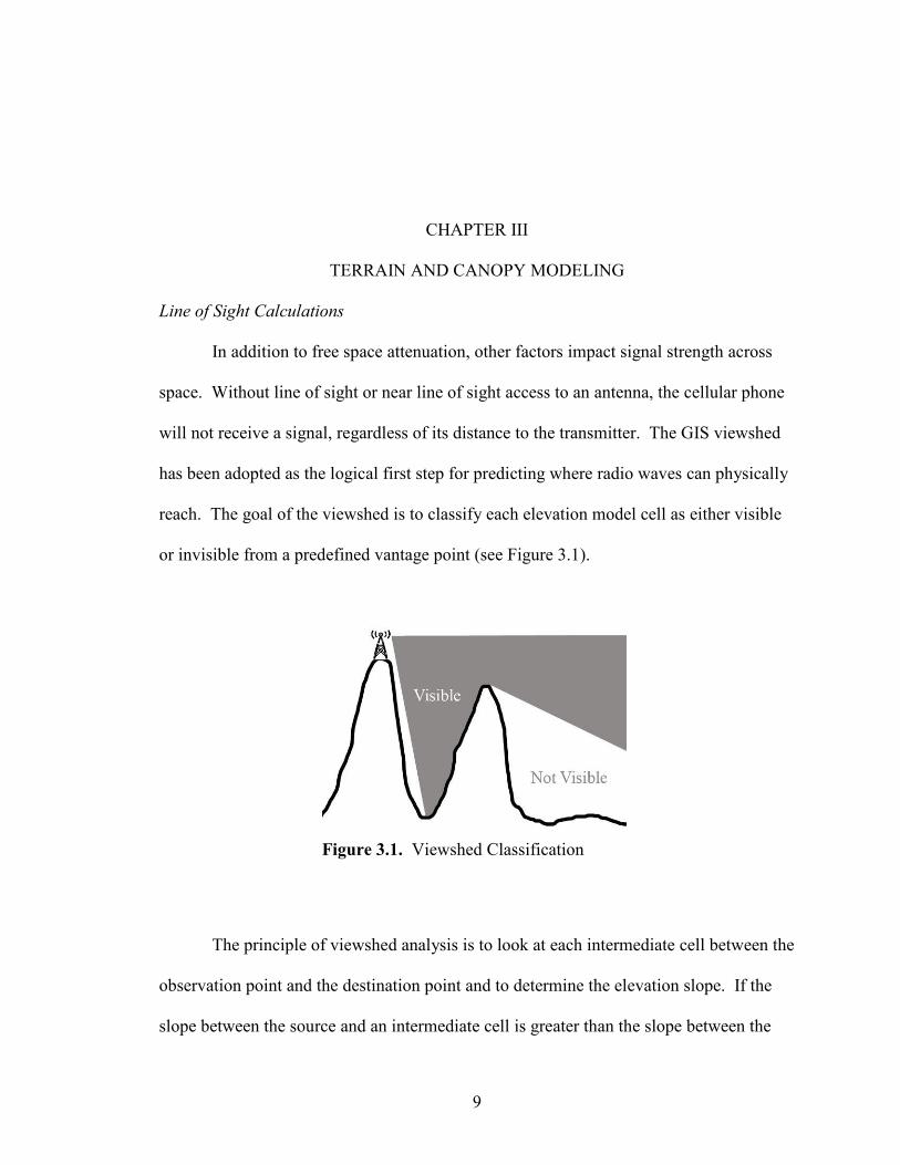
Line of Sight Calculations

In addition to free space attenuation, other factors impact signal strength across

space. Without line of sight or near line of sight access to an antenna, the cellular phone

will not receive a signal, regardless of its distance to the transmitter. The GIS viewshed

has been adopted as the logical first step for predicting where radio waves can physically

reach. The goal of the viewshed is to classify each elevation model cell as either visible

or invisible from a predefined vantage point (see Figure 3.1).

The principle of viewshed analysis is to look at each intermediate cell between the

observation point and the destination point and to determine the elevation slope. If the

slope between the source and an intermediate cell is greater than the slope between the

Figure 3.1. Viewshed Classification

10

source and the destination, then the view must be at least partially blocked (Sorenson and

Lanter 1993). Either a raster or vector model can be used in such an analysis.

Light Detecting and Ranging (LIDAR) data has been increasing in popularity as

an alternative to the photogrammetrically-derived USGS DEMs. A LIDAR system

mounted on an aircraft will measure the time it takes a pulse of laser to hit the earth and

return backscatter. The more laser pulses emitted from the aircraft, the higher the

resolution of the subsequent elevation model. The USGS photogrammetrically-derived

topographic maps claim a vertical accuracy of half of one contour interval (5 feet for 10-

foot contour lines) for 90% of the points surveyed (USGS 2006). In contrast, LIDAR-

derived DEMs boast accuracies as small as 7 cm (NCFM 2003).

In addition to its high accuracy level, another benefit of this technology is its

ability to measure both ground and canopy heights simultaneously. As the scanner

measures the backscatter of the laser pulses, multiple returns from the same laser pulse

will indicate multiple levels of ground cover. The first return reflects the elevation of the

top of the canopy, while the last return generally indicates the ground elevation (Roberts

et al. 2004; Hyde et al. 2006). There will also be last returns which never reach the

ground, bouncing off buildings, tree trunks, and other ground clutter. These points can be

differentiated from ground points using filtering algorithms.

Several filtering algorithms have been proposed to eliminate false ground

readings. Most operate on the conservative premise that since these scanners are so

prolific in their number of returns, throwing out some good returns along with the outliers

is better than leaving outliers in the dataset. Since wooded areas have an abundance of

11

problematic points above the ground, the result can be the removal of most of the points

by the end of the filtering algorithm.

In the filtering process, both falsely high and falsely low readings must be

eliminated. Falsely high elevation values are largely due to canopy obstructions. Falsely

low elevation values are a result of multipath. If part of the emitted energy bounces

between surfaces before returning to the scanner, the scanner will calculate a value that

actually lies below the earth’s surface.

Most filtering algorithms are based on the principle that drastic height changes

between two relatively close LIDAR points are suspicious. Some algorithms use slope as

a measure (Zhang et al. 2003; Zaksek and Pfeifer 2006; Kilian et al. 1996). Others use

the principle of linear prediction, in which strong outliers are iteratively removed until a

good approximation of the ground is obtained (Kraus and Pfeifer 1998). Yet another

group of methodologies involves segmentation of the terrain. Using region growing

principles, the LIDAR point cloud is divided into segments representing various terrain

and canopy elements such as buildings, trees and ground. The assumption is that, at the

end of the procedure, the largest segment must be the ground (Jacobsen and Lohmann

2003; Verma et al. 2006). A few years ago Sithole and Vosselman set out to evaluate

various algorithms. They discovered that the segmentation method was most robust

(2004). However they concluded that in wooded areas with steep terrain all the

algorithms tended to fail, including segmentation.

Kobler et al. chose to develop an algorithm suited to wooded areas with steep

terrain (2007). Their resulting technique is called repetitive interpolation (REIN). First

12

the strongly positive and negative outliers are removed from the data. Citing previous

research showing that an intelligent analyst can remove outliers through simple

observation (Sithole and Vosselman 2004), they recommend visually removing the

obvious errors. To remove additional outliers, the slope between each point and its

nearest neighbor is calculated. Those points with slopes significantly higher than the

steepest slope expected in the area are eliminated. In the final filtering stage, independent

random samples are taken from the LIDAR data. An elevation model is created from

each sample. The result is a distribution of elevations at each location in the model.

Since LIDAR data is most plagued with positive canopy outliers, the lowest elevation at

each point is assumed to be closest to the truth. An adjustment value called the global

mean offset (gmo) is calculated based on the differences between the independent random

sample interpolations. The gmo is added to the minimum elevation at each point to

determine the elevation value of the final output terrain model (Kobler et al. 2007).

Whatever the algorithm used to determine the ground elevation points, a choice

must be made about the spatial resolution of the output DEM. A balance needs to be

struck between the necessary accuracy and the processing time. The more points

included in the interpolation, the greater the accuracy and the longer the processing time.

Anderson et al. proposed solutions for determining the best mix of accuracy and data

reduction (2006). In their study they performed random data reduction methods. After

each data reduction and subsequent interpolation, they compared the output to a DEM

created from the entire set of points. They show that a 5-meter DEM with about 143 data

points per hectare (representing 50% of their original dataset) will not be statistically

13

different from a 5-meter DEM created from 100% of the points. On the other hand, only

40 data points per hectare would be necessary (10% of their original dataset) to create a

similar 30-meter DEM. Anderson et. al. showed that it is valid to randomly select a

portion of the entire dataset to create a DEM in a fraction of the time.

Tree Canopy Model

Using all returns LIDAR data, it is possible to create an elevation grid

representing the ground in addition to a grid modeling the upper tree canopy. Such grids

are typically made through linear interpolation of the LIDAR points, potentially yielding

a vertical accuracy as small as 0.5 m (Roberts et al. 2004; Hyde et al. 2006). This

technique is best employed with LIDAR collected in leaf on conditions. It remains to be

seen if leaf off LIDAR could produce a canopy model approximating the ground truth.

The benefit of a canopy model for this research would be the incorporation of a

new independent variable – distance through ground clutter. In the past, the vegetation

ground clutter values used in propagation algorithms have been absolute numbers

(Rubinstein 1998). Some work has been done testing construction materials for

determining building penetration (Rappaport 2002), however this type of research has not

yet been widely extended to rural features like forests. Schwering et al. made some

observations of which frequencies better penetrate vegetation (1988), but made no

inferences that could be incorporated into a robust computer model.

If GIS could be used to model the distance traveled through the vegetation

canopy, research could determine clutter in terms of dBm’s lost per meter. The

14

assumption is that the attenuation of the wave should be less severe on the edge of a

forest than several meters into the forest (Schwering et al. 1988). Modeling the canopy

cover would produce new opportunities to examine radio wave behavior.

Diffraction Estimates

Unfortunately line of sight using the viewshed analysis does not give a complete

picture of cellular coverage. Diffraction not only allows radio waves to travel across the

curved surface of the earth, but it also gives radio waves the ability to propagate around

obstacles to some extent. These areas outside the line of sight are called “shadowed.”

The signal strength will rapidly decrease in these shadowed regions, but often enough

useful signal will still remain (Rappaport 2002). Some simple situations can be

calculated, among which are knife-edge diffraction and multiple knife-edge diffraction

(Deygout 1966; Bullington 1947; Epstein and Peterson 1953). Signal strength

approximations can be made from these cases and applied to a propagation model.

Tx = Transmitter, Rx = Receiver

Figure 3.2. Multiple Knife-Edge Diffraction

15

One of the most widely-used diffraction algorithms was described by Deygout in

1966. He presented a formula that could be used iteratively for multiple obstructions.

Figure 3.2 shows an example of two obstructions. Deygout’s method is to first compute

the diffraction loss of the main obstacle (path TxM1Rx in Figure 3.2). The next step is to

compute the secondary diffraction loss by applying the same calculations to the path

M1M2Rx. Those loss values are added together. Finally, a correction factor is

incorporated into the equation, completing the total diffraction loss calculation (TDL).

TDL = ML + SL - TC

16log201

1 +

=

rh

ML

where )(

)(5481 cbaf

cbar ++

+=

16log202

2 +

=

rh

SL

where )(

)(5482 cbaf

bacr ++

+=

p

p

qTC

2

1

2log2012

−−=

πα

where ac

cbab )(tan

++=α

where 21

1

r

hq = and 2

2

2

r

hp =

f = frequency of the signal

λ = wavelength of the signal

Equations 3.1.1 to 3.1.8 show the complete set of calculations involved in computing

TDL.

(3.1.1)

(3.1.2)

(3.1.3)

(3.1.4)

(3.1.5)

(3.1.6)

(3.1.7)

(3.1.8)

16

Some say it is not possible to accurately model the diffraction losses that occur

from terrain. For this reason many researchers choose to omit diffraction effects from

their studies, eliminating all shadowed areas from their results (Schwering et al. 1988;

Dal Bello et al. 2000). Deygout defends his diffraction methodology as sound in his

1991 paper. Based on applying his own algorithms for 21 years, he asserts that the mean

error of his cumulative data collection is 1 dB, with a standard deviation of 4-5 dB. He

speculates that the errors people tend to have with his methodology are largely due to

inaccurate terrain models. He notices that the greatest errors tend to occur with the

greatest transmitter-receiver separation. Since his methodology is iterative, each error in

the elevation of an obstruction compounds, generating gross errors at far distances.

17

CHAPTER IV

AVAILABLE DATA

Cell Phone Tower Data Set

A confidential cell phone tower data set was obtained for one Provider for the

state of North Carolina. All locations are for digital towers, which fall in the 1850 to

1990 MHz range. The towers are divided into sectors, with three per tower in most cases.

The data set consists of latitude and longitude in the datum World Geographic System

(WGS) 1984, antenna heights and sector azimuths. Most antennas for Provider have

three sectors with azimuths 120 degrees apart. By having three sectors, the antenna

achieves coverage approximating the shape of a circle. The azimuth is measured in

degrees from north. Figure 4.1 shows a typical antenna propagation pattern with sector

azimuths 120 degrees apart.

Figure 4.1. Three Sector Antenna

Propagation Pattern

18

Figure 4.2. Geographic Research Area

19

An area of interest was chosen just north of Bryson City, North Carolina. The

park refers to this area as Deep Creek. Three Provider towers impact this area, with their

locations shown in Figure 4.2. The towers vary in height and elevation, while each

supports three sectors at azimuths 0, 120 and 240.

LIDAR Data Set

An all returns LIDAR data set for the area of interest was obtained from the North

Carolina Floodplain Mapping Program. This LIDAR was flown at the beginning of 2005

in leaf off season to facilitate the acquisition of bare earth data, particularly in forested

areas (NCFM, 2006). Earthdata International performed a proprietary filtering of the data

points. An independent accuracy assessment found that the DEMs generated from the

filtered LIDAR points located in the park had an RMSE of 1.42 ft (0.43 m), with the

standard deviation of the vertical errors being 1.44 ft (0.44 m) (NCFM 2006).

Vegetation Classification Data Set

A classified map of the Great Smoky Mountains National Park was obtained from

the National Park Service (NPS). The NPS Vegetation Map is comprised of forty classes.

Each class is a combination of over- and undercanopy types. The NPS began its

vegetation mapping in the Cades Cove and Mount Le Conte quads because they believe

the vegetation contained in these regions to be representative of the diversity of the park

(ESRI 2000). The classification was supervised, involving the advance collection of field

observations prior to photointerpretation (The Nature Conservancy 1999). The remainder

20

of the park was classified by comparing a variety of aerial imagery to the classes in the

pilot quads. The park finished its accuracy assessment at the beginning of 2007. They

estimate the overall accuracy of the map to be 80%. The assessment points collected

within the area of interest had a lower accuracy of 78% (Jenkins 2007).

21

CHAPTER V

METHODOLOGY

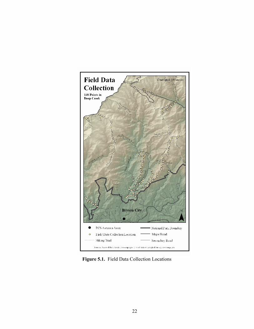
Field Data Collection

Field measurements were conducted along the trails of the Deep Creek region,

located north of Bryson City and south of Clingman’s Dome. It was determined that

three towers could be impacting this area based on their distances and elevations. As this

research is interested in visualizing the reception hikers can expect in the park, data

collection was conducted along the roads and trails. A stratified random sample of trail

segments was selected representing approximately 20% of the trails within the area of

interest. Using a 10-meter DEM acquired from the USGS, a preliminary viewshed

showed which trails had areas within the line of sight and which trails were completely

outside the line of sight. Half the sample was taken from each of these categories in

order to ensure that measurements would include trails within the line of sight for post

processing.

The FCC Universal Licensing System was consulted to determine the frequency

bands reserved by Provider in the geographic area of interest. Two band widths were

reserved in the area, 1870-1885 MHz and 1950-1965 MHz. A spectrum analyzer survey

of the three antenna sites concluded that each of these antennas was operating within the

1950-1965 MHz band.

22

Figure 5.1. Field Data Collection Locations

23

Along each randomly selected road or trail, measurements were taken at equal

intervals, approximately 300 meters apart. A total of 148 points were visited. At each

point the following data were collected: GPS coordinates, and received signal power. At

73 of the 148 locations, the approximate tree canopy height was also measured. The GPS

device had a horizontal accuracy of one meter and an estimated vertical accuracy of two

meters. The tree canopy heights were calculated using a clinometer to measure the height

of a typical tree in the area. The accuracy of this methodology is approximately 4 meters.

The received signal level measurement had an accuracy of 3 percent according to

equipment specifications. Figure 5.1 shows the locations of each data collection point.

Elevation Model Creation

The all returns LIDAR data from the North Carolina Floodplain Mapping Program

was divided into two data sets – last returns and first returns. All points with the same

geographic coordinates were separated between the maximum elevation and the

minimum elevation. The data was then evaluated for outliers. Typical outliers are first

returns that capture birds, clouds, or any other elevation that is above the ground canopy

(Hyde et al. 2007). Any point greater than 100 meters above or below others in the

geographic vicinity was eliminated by a visual survey.

The minimum elevation does not necessarily represent the ground level, as tree

crowns may stop the signal entirely before it hits the ground. With this situation in mind,

the minimum elevation values were further filtered according to the methodology devised

by Kobler et al. (2007). Six independent random samples with replacement were taken

24

from the last returns dataset, each representing 23% of the entire dataset. The resulting

six sample datasets had an average of 145 points per hectare. According to Anderson et

al., at least 143 points per hectare can be used to create a 5-meter DEM (2006). They

determined that a smaller cell size would result in unnecessary computer processing time

with no additional accuracy. Each of the six samples was interpolated to a 5-meter DEM

using the inverse distance weighting algorithm.

These grids were processed to obtain a local minimum for each grid cell in the

area of interest. The output grid containing the local minimums was then used along with

the six sample grids to calculate the gmo. The local gmo for each cell is represented by

the average differences across all six grids (Equation 5.1).

dij = zij – zj,min

Where zij is the i-th elevation estimate at the j-th location

and zj,min is the lowest elevation estimate at the j-th location.

The gmo for the entire dataset is the average of all the local gmo’s. The gmo for the area

of interest was calculated to be 1.83 meters. The gmo was added to each cell in the

minimum elevation grid to produce the final REIN elevation grid.

This methodology was repeated with the first returns, to create five sample grids.

The maximum, instead of the minimum, was calculated at each grid cell location.

Similarly the gmo (2.7 m) was subtracted from the maximum elevation grid to produce a

final canopy grid. Kobler et al. did not test the REIN algorithm as a methodology for

creating a tree canopy model (2007). Therefore an error analysis will be key in

determining the usefulness of the canopy grid.

(5.1)

25

Predicted Signal Strength Calculations

In order to obtain a predicted signal strength for each field collected point, the

first step was to calculate the free space loss. If the transmitted power level of the

antenna is known, the Friis free space formula (Equation 2.1) can be used to approximate

the amount of power remaining in the radio wave when it reaches the receiver.

Unfortunately Provider did not respond to inquiries related to the power level of their

antenna systems. Therefore additional field work was conducted to create a reference

point from which additional free space calculations could be derived. If the researcher

has a known power level at a known distance from the antenna, additional power values

can be calculated relative to that reference power level (Molish 2005, Rappaport 2002).

Equation 5.2 shows that the measured power from a reference distance Pr(d0) can be used

to predict the signal power at another distance from the antenna.

2

0

0 )()(

=

d

ddPdP rr d ≥ d0 ≥ df

Pr = receiver power in milliwatts

d = transmitter-receiver separation in meters

d0 = received power reference point

where df = 2D2 / λ

and D = largest physical linear dimension in meters

on the transmitter antenna

Tables 5.1 and 5.2 show the results of the measurements taken to calculate the reference

power of each transmitter. An average was taken of the measurements around each tower

and used in Equation 5.2 as d0. Using this value combined with the actual distance

(5.2)

26

Table 5.1. Measurements for Reference

Power Calculation

Tower Received Signal

Levels (dBm) at 1 km

Bryson City -50.4

-58.4

-61.2

-60.0

-76.8

-68.4

Sylva -70.8

-81.6

-61.2

-69.2

-79.2

-87.2

-66.0

-73.2

-75.2

-67.2

-63.6

-71.2

Franklin -67.2

-70.4

Table 5.2. Reference Power Values

Tower Average

Power in dBm

at 1 km

Average

Power in mW

at 1 km

Bryson City -62.5 5.62 x 10-7

Sylva -73.1 4.90 x 10-8

Franklin -68.8 1.32 x 10-7

Figure 5.2. Sample Profile Between Transmitter and Receiver

27

separations, Pr(d) was evaluated for each point from the perspective of each tower,

resulting in three predictions at each site.

The output ground elevation DEM from the LIDAR analysis was then input into

Cellular Expert along with the locations and heights of the towers of interest. A profile

was created between each tower and each data point (see Figure 5.2). Each profile shows

how far the radio wave would travel and the location and height of each terrain obstacle.

Most importantly, the profile also calculates the Deygout diffraction for each path. The

Deygout diffraction value was added to the free-space value, resulting in a loss prediction

including terrain as a variable.

Three predictions were available for each data collection point, accounting for the

independent variables of frequency, distance and terrain. The received signal level

measurements collected in the field represented the strongest signal available within that

bandwidth at that location. Therefore the highest of each of the three predicted values

was gleaned from the calculations for comparison to the field collected data. Differences

between observed and measured values were analyzed, with the hopes that the residuals

could be attributed to land cover attributes.

28

CHAPTER VI

ANALYSIS AND RESULTS

Accuracy Assessments

GPS Terrain Heights

The REIN terrain elevation grid was assessed for accuracy based on the GPS

collected points from the field data collection. The average absolute error between the

GPS readings and the REIN grid was 4.17 meters, and the standard deviation 4.44 meters.

A histogram of the elevation errors is shown in Figure 6.1. The skewness is -0.391,

indicating that the mass of the distribution is concentrated on the right side of the

histogram. This would indicate that more often than not, the observed value was greater

than the value predicted by the REIN grid. An average absolute error of 4.17 meters is

greater than expected considering the 0.43 m accuracy asserted by the North Carolina

Floodplain Mapping Program. However the observed values being more often greater

than predicted values could indicate that the REIN algorithm did what it claimed, in that

it eliminated the impact of tree crowns from the final DEM.

29

Over-Canopy Grid

Next the REIN canopy elevation grid was assessed for accuracy based on the

clinometer calculations of an average tree at 73 GPS collected points. The average

absolute error between the clinometer readings and the REIN grid was 10.08 meters, and

the standard deviation 6.55 meters. A histogram of the elevation errors is shown in

Figure 6.1. The skewness is -0.141, indicating that the mass of the distribution is slightly

concentrated on the right side of the histogram. This would indicate that more often than

not, the observed value was greater than the value predicted by the REIN grid. Only 7

points were over-estimated by the model, while 93 points were underestimated by the

model. Therefore for 89% of all the points, the canopy grid gave a value lower than the

20.0000000000010.000000000000.00000000000-10.00000000000-20.00000000000-30.00000000000

Frequency

50

40

30

20

10

0

Error

Figure 6.1. Histogram of Elevation Errors

(Observed Minus Predicted)

30

ground truth. This would indicate that despite the density of the trees in this area, LIDAR

points collected in leaf off conditions are not sufficient for creating a canopy grid using

the REIN algorithm.

Signal Strength Calculations

The noise floor published in the specifications of the spectrum analyzer is -110

dBm. As the signal approaches -110 dBm, the likelihood increases that the any reading

would only reflect environmental noise or noise internal to the unit. Close to -108 dBm,

the cell phone tower signal becomes indiscernible from that noise. Therefore any signal

strength that was recorded as less than -108 dBm is suspect. In such a case the truth

could be -108 dBm, or the truth could be lower. It would be impossible to tell with this

set of equipment. In order to avoid this type of suspect data, all observations less than

0.00000000 10. 00000000 20. 00000000

0

5

10

15

Count

Error

Figure 6.2. Histogram of Canopy Height Errors

(Observed Minus Predicted)

31

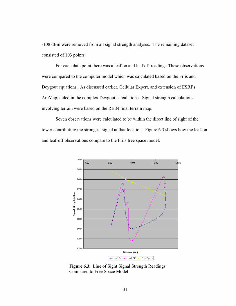
-108 dBm were removed from all signal strength analyses. The remaining dataset

consisted of 103 points.

For each data point there was a leaf on and leaf off reading. These observations

were compared to the computer model which was calculated based on the Friis and

Deygout equations. As discussed earlier, Cellular Expert, and extension of ESRI’s

ArcMap, aided in the complex Deygout calculations. Signal strength calculations

involving terrain were based on the REIN final terrain map.

Seven observations were calculated to be within the direct line of sight of the

tower contributing the strongest signal at that location. Figure 6.3 shows how the leaf-on

and leaf-off observations compare to the Friis free space model.

Figure 6.3. Line of Sight Signal Strength Readings

Compared to Free Space Model

32

In five of the seven cases, the measured value was less than the free space value.

This follows the hypothesis that field collected measurements within dense vegetation

would be lower than a free space calculation. It is interesting to note that the two last

anomalous points are both much farther from their antenna than the other five.

Figure 6.4 shows how closely the field measurements came to the ideal predicted

value for all 103 cases. It shows that as the predicted signal strength decreases, the gap

between the model and the reality increases. The mean leaf-on error was -37.6, while the

mean leaf-off error was -40.3. The standard deviations were similar, 27.5 and 28.6

-200.0

-180.0

-160.0

-140.0

-120.0

-100.0

-80.0

-60.0

-40.0

-20.0

0.0

-200.0 -180.0 -160.0 -140.0 -120.0 -100.0 -80.0 -60.0 -40.0 -20.0 0.0

Free Space Plus Diffraction Model Value (dBm)

Signal Strength Value (dBm)

Leaf On Leaf Off Ideal Model Linear (Ideal Model)

Figure 6.4. Ideal Free Space Plus Diffraction Model Compared to

Observed Values

33

respectively. Both have a -0.7 skewness, showing once again that the observed values

tended to be greater than the predicted values (See Figure 6.5).

The ideal model compared well in cases where diffraction around ridges was not a

factor. However the ideal model did not do nearly as well in the other 96 cases where

Deygout diffraction was calculated. Since the elevation model had an average error of

about 4 meters, it is probable that the prediction accuracy was strongly impacted by the

quality of the REIN grid. This problem, documented by Deygout and his critics has

created an experimental obstacle here as well (Deygout 1991). The proposed

methodology was to compute free space and diffraction for each point, then to assume

that the difference between that computation and reality was solely due to other variables.

Without conducting much more extensive field measurements, it is impossible to know

the exact elevation of each ridge which lies between each point and its antenna. The

-120.00 -80.00 -40.00 0.00

Leaf On Error

0

5

10

15

Count

-120.00 -80.00 -40.00 0.00

Leaf Off Error

0

5

10

15

20

Count

Figure 6.5. Ideal Free Space Plus Diffraction Model Error, Leaf On and Leaf Off

34

relative inaccuracy of the terrain model now renders this approach impossible since the

data are not available at this time to have an accurate Deygout calculation for each point.

Vegetation Classification

In classifying the Great Smoky Mountains National Park, the National Park

Service used the Community Element Global Codes (CEGL) from the National

Vegetation Classification Standard. Since the vegetation of this area is among the most

diverse in the world, the ecologists found that certain CEGL classes were prone to be

misconstrued. Although they observed 58 distinct CEGL classes, they chose to combine

several classes that were indistinguishable in the remotely sensed data. The result was 40

distinct classes, 31 of which are CEGL classes, and the remaining 9 of which fell outside

this classification system (ex. roads, rock, gravel, etc.).

For the current data analysis, the remaining 31 CEGL classes were consolidated

into four distinct categories: evergreen, northern hardwood, oak-hickory, and cove

hardwood. The polygons which fell outside the classification system were invariably

small. For the sake of analysis, the closest class within the NPS system was observed and

applied. Table 6.1 shows how the NPS classes contained in the AOI were consolidated to

become four analysis classes.

Of the 103 points remaining in the sample, 11 were evergreen, 18 were northern

hardwood, 69 were oak-hickory, and 6 were cove hardwood. Table 6.2 shows the

distribution of the points compared to the actual distribution of the vegetation classes

within the area of interest. In this table the population statistics include the entire area of

interest, whereas the data collection points were limited by trail access.

35

Table 6.1. Consolidation of Analysis Categories

Analysis Categories NPS Code

Evergreen

250 – 2000m elevation, mesic soil

Includes formerly mixed spruce-fir forests, where some or

nearly all the firs have been killed by the balsam wooly

adelgid. Evergreen areas with pine also include various

kinds of oak and hickory.

1013 – spruce-fir

1001 – yellow pines

7517 – eastern white pine

Northern Hardwood

1000 – 1500m elevation, mesic soil

Traditionally birch, beech and buckeyes. Birch is most

prolific, but also has spruce, hemlock and red maple.

6124 – forested boulderfield

1010 – northern and acid hardwoods

1011 – northern hardwoods and

boulderfields

Oak-Hickory

250 – 1500m elevation, sub-mesic soil

Various kinds of oak and hickory, with some birch and red

maple.

6192 – oak hardwood with red maple

7230 – oak hardwood with hickory

7692 – oak hardwood rich type

1007 – chestnut oak

1008 – high elevation beech and red oak

1009 – high elevation red and white oak

Cove Hardwood

250 – 1000m elevation, mesic soil

Maple, tuliptree and birch abound. Hemlock is fairly

common.

7543 – cove hardwood acid type

7710 – cove hardwood typic

1003 – floodplain forest

1006 – successional hardwood

Table 6.2. Distribution of Sample by Vegetation Analysis Class

Analysis Category Sample Frequency

(# of points)

Sample

Percent

Population

Frequency (ha)

Population

Percent

Evergreen 11 10.6 2,352 10.1

Northern Hardwood 18 17.3 6,238 26.7

Oak-Hickory 69 66.3 9,828 42.1

Cove Hardwood 6 5.8 4,947 21.2

TOTAL 104 100 23,365 100

For each of its vegetation classes, the park has an inferred soil moisture category

(Madden 2004). Those categories were recorded for each NPS code and related to each

data collection point. They describe the overall moisture trends of that particular

vegetation class across time. The high moisture category gets plenty of precipitation in

prime growth times. The low moisture category gets much less precipitation, and the

little it gets is in the winter.

36

Statistical Analysis

The differences between observed and predicted signal strength values proved to

be great, and could probably be attributed to the quality of the terrain modeling.

Although it may not be possible at this time to attribute all the residuals to land cover

variables, it is still useful to look at how the environmental attributes could have

contributed in part to the signal strength measurements. To that end, three sets of

comparisons were run. Each one assessed the contributions that the land cover variables

made to leaf on measurements, leaf off measurements and the difference between local

leaf on and leaf off measurements. Independent variables included vegetation type, soil

moisture content, measured tree canopy height, and distance from the dominant antenna.

ANOVA Tests

ANOVA tests were run to test the impact of the independent variables of

vegetation type and soil moisture content on the signal strength measurements. The soil

moisture levels reported by the NPS were nominal, distinguishing between dry, wet and

medium soil types. As seen in Table 6.3, the only significant result seen in these

ANOVAs is the impact of soil moisture on the difference between leaf on and leaf off

measurements. Figure 6.6 shows the differences in means graphically. While the

medium and low moisture categories had similar means, the high moisture category was

significantly different.

There was no significant difference in means between the four vegetation

categories and the difference between the leaf on and leaf off measurements. The

ANOVA results for this test are shown in Figure 6.7.

37

Table 6.3. ANOVA Test Results With Signal Strength as the Dependent Variable

Dependent Variables Independent Variables

Vegetation Type Soil Moisture

F-Value P-Value F-Value P-Value

Leaf On Signal Strength 0.66 0.5790 0.24 0.7860

Leaf Off Signal Strength 2.58 0.0582 2.30 0.1054

Leaf Off – Leaf On 2.09 0.1061 5.83 0.0041*

* p-value is significant (α = 0.05)

High,

0.083

Low,

5.4

Medium,

3.577

0

1

2

3

4

5

6

Soil Moisture

Leaf Off - Leaf On (dBm)

Figure 6.6. Soil Moisture as the Main Effect for the Difference Between Leaf Off

and Leaf On Measurements. The different symbols indicate a significant difference

between each category.

38

In order to test the possibility of the independent variables being correlated in

some way, ANOVAs were also run testing the impact of vegetation type and soil

moisture content on tree canopy height and distance from the dominant antenna. The

results are shown in Table 6.4. Significant differences in means were found in all cases.

Tree canopy height varies by vegetation type and by soil moisture, while distance also

varies by vegetation type and soil moisture. Figures 6.8 and 6.9 graphically show the

difference in means of the tree canopy heights, with vegetation type and soil moisture

respectively as the main effects.

Oak-

Hickory,

3.722

Evergreen,

1.44

Cove

Hardwood,

2.533

Northern

Hardwood,

0.044

0

1

2

3

4

5

6

Vegetation Class

Leaf Off - Leaf On (dBm)

Figure 6.7. Vegetation Class as the Main Effect for the Difference Between Leaf Off

and Leaf On Measurements.

39

Table 6.4. ANOVA Test Results With Tree Canopy Height and Distance from

Dominant Antenna as the Dependent Variables

Dependent Variables Independent Variables

Vegetation Type Soil Moisture

F-Value P-Value F-Value P-Value

Tree Canopy Height 6.00 0.0040* 7.46 0.0080*

Distance from Dominant Antenna 8.12 <0.0001* 11.32 <0.0001*

* p-value is significant (α = 0.05)

Oak-

Hickory,

15.662

Evergreen,

8.214

Cove

Hardwood,

14.557

Northern

Hardwood,

9.558

0

2

4

6

8

10

12

14

16

18

Vegetation Class

Canopy Height (m)

Figure 6.8. Four Vegetation Classes as the Main Effect for the Measured Canopy

Height. The different symbols indicate a significant difference between each category.

40

Correlation Tests

Since the independent variables of tree canopy height and distance are

interval/ratio data types, it was possible to use a correlation to test their relationship to

signal strength. Table 6.5 shows that a significant negative correlation exists between

leaf off signal strength and distance. Tree canopy height has a positive correlation to the

leaf on leaf off difference, however distance has a negative correlation to the leaf on leaf

off difference. For every meter the tree canopy increases, the signal strength gap

increases by 0.283 dBm. Conversely, for every meter the transmitter-receiver distance

increases, the signal strength gap decreases by 0.290 dBm.

Med,

15.622

Low,

13.055High,

9.768

0

2

4

6

8

10

12

14

16

18

Soil Moisture

Canopy Height (m

)

Figure 6.9. Soil Moisture as the Main Effect for the Measured Canopy Height. The

different symbols indicate a significant difference between each category.

41

Table 6.5. Correlation Test Results With Signal Strength as the Dependent Variable Dependent Variables Independent Variables

Tree Canopy Height Distance

R-Value P-Value R-Value P-Value

Leaf On Signal Strength -0.108 0.3638 -0.085 0.3915

Leaf Off Signal Strength 0.106 0.3710 -0.298 0.0022*

Leaf Off – Leaf On 0.283 0.0154* -0.290 0.0030*

* p-value is significant (α = 0.05)

The possibility of a correlation between distance and tree canopy height was

investigated. The r-value was -0.210, indicating a potential negative correlation.

However the p-value was 0.0742, which is not small enough to indicate a significant

relationship between the two variables.

Discussion of the Results

There were few significant findings relating the independent variables directly to

the field measured values. None of the independent variables significantly impacted the

leaf on measurements. Distance was found to be the only significant predictor of leaf off

measurements, with a p-value of 0.0022. Not surprisingly, the closer the receiver, the

higher the signal strength. In light of that finding, it is interesting to note that distance

was not a significant predictor of leaf on signal strength. This lack of significance

actually bolsters the hypothesis that leafy vegetation does indeed play an independent

role on signal attenuation.

An analysis of the differences between the seasonal values at each data collection

point reaped the most interesting results. There was no significant difference in means

between the four vegetation categories. Figure 6.7 shows that although at face value the

four classes appear to be different, the p-value for the ANOVA was 0.1061.

42

If the vegetation categories were to be consolidated into two classes, a different

story would emerge. Figure 6.10 shows that there is a significant difference in means

between the two categories of Northern Hardwood and Evergreen, and Oak-Hickory and

Cove Hardwood.

The first category is dominated by spruce, fir, pine, beech, birch and red maple.

The second category is dominated by various types of oak (red, white and chestnut), tulip

poplar, and hickory. These categories might seem arbitrary, but they are actually

connected to other environmental characteristics. The first category has an average

Oak,

Hickory and

Cove

Hardwood,

3.627

Northern

Hardwood

and

Evergreen,

0.207

0

1

2

3

4

5

6

Vegetation Class

Leaf Off - Leaf On (dBm)

Figure 6.10. Vegetation Class as the Main Effect for the Difference Between Leaf On

and Leaf Off Measurements. The different symbols indicate a significant difference

between each category.

43

canopy height of 9 meters, while the second has an average canopy height of 15 meters.

The ANOVA showing the effect of the vegetation category on canopy height shows that

Northern Hardwood and Evergreen as a group have significantly different canopy heights

than Oak-Hickory and Cove Hardwood (Figure 6.8). This trend implies that canopy

height by itself could tell more of the story than tree species.

A correlation comparing the measured canopy height to the seasonal differences

showed a significant positive correlation of 0.28, with a p-value of 0.0154. The higher

the canopy, the more the signal improved in the winter. For every meter increase in the

canopy, the signal improved by 0.28 dBm when the leaves fell.

Distance was also found to be a predictor of the magnitude of the change between

leaf on and leaf off. A negative correlation of -0.29 was found between the two, with a p-

value of 0.003. For every meter increase in distance between the antenna and the

receiver, the gap between leaf on and leaf off diminished by 0.29 dBm. Since there was

no significant correlation between canopy height and distance, distance could be having

its own unique impact on the signal. The farther the distance, the less the leafy

vegetation impacts further attenuation.

Finally, soil moisture was found to have a significant impact on the leaf on v. leaf

off difference. It was also shown to be linked to tree canopy height and distance. It is

unlikely that distance from the antenna is plays a direct role in the composition of the

soil, or in the signal strength differences. In all the studies that have looked at distance as

a variable, one was not found that correlated short distances with the potential for high

clutter interference. It is possible that a causal connection exists between soil moisture

44

and tree height. How the soil moisture and canopy height combine to predict signal

strength loss is not entirely clear. The higher the moisture content, the less the signal

strength gap. The higher the canopy, the more the signal strength gap. The higher the

soil moisture, the lower the canopy. The results seem counterintuitive. They may have

been impacted by the number of observations in each class. Whereas high and medium

moisture contain 29 and 71 points respectively, low only holds 4 sample points. Soil

moisture could also easily be a barometer for another environmental variable not

considered here.

45

CHAPTER VII

CONCLUSION

Up to this point radio propagation research involving vegetation has focused on

determining differing loss values for different tree species. This study has uncovered a

significant new angle of research, indicating a need to focus on other environmental

attributes. Significant relationships were found relating soil moisture and tree heights to

attenuation. According to the data collected, the height of the tree canopy was a more

significant contributor to attenuation than the species of the tree. In fact, the vegetation

classes were not found to be indicators at all until they were grouped according to mean

heights. In this study the species of tree was only significant insomuch as it was an

indicator of the tree height.

In light of this discovery it was disappointing that the tree canopy grid proved to

be inadequate for modeling. Leaf on LIDAR data would certainly yield a much better

digital model, however this data is harder to find and often has not been collected. An

alternative to creating a model through LIDAR would be to use generalized tree height

data regularly collected by the National Park Service and other entities. Each vegetation

category could be given an approximate canopy height to input into a path loss

calculation.

The soil moisture variable deserves further consideration in future studies. It is

unlikely that the soil in an of itself is impacting signal loss. It is much more plausible

46

that the soil moisture content is impacting other aspects of the physical environment.

This study did not differentiate between successional and old growth forests.

Successional forests are going through a process of regrowth. They can have plenty of

annual precipitation but a low canopy of young tree stands. If a correlation were found

between successional forests and high soil moisture, that might account for the finding

that moisture impacts signal attenuation. It is also possible that the undercanopy is

playing a role, as bushes were often taller than the height of the field data collection

equipment. The makeup of the undercanopy can also vary according to the precipitation.

Ideally further studies would include a greater volume of points within the line of sight of

the antenna. Removing the variable of terrain diffraction could help clarify some of these

questions.

Finally, in the interests of creating excellent propagation maps without the need

for expensive field data collection, greater attempts should be made to improve the

accuracy of elevation modeling in this context. Different algorithms for LIDAR filtering

could yield improved diffraction calculations. There is value in comparing the

performance of various LIDAR filtering and terrain modeling techniques.

Every improvement of wireless modeling in rural settings is a step toward a better

understanding of how radio waves interact with the environment. Improved

understanding creates better management of resources and minimization of the visual

impact of towers. As urbanization continues to eliminate green spaces in the United

States, the popularity of park recreation will only increase. Concerns over safety have

always been and will continue to be an issue in the future. Rural areas experience the

47

same public health and emergency concerns as urban areas. Popular recreation spots with

regular incidents and poor coverage are particularly disadvantaged in the face of a crisis.

Predicting cell phone coverage for wilderness areas frequented by novice hikers

makes good sense. The National Park Service has grown in the last hundred years from a

few hundred thousand visits to 275 million visits each year (NPS 2007). Incidents will

happen. An understanding of how to predict and visualize wireless coverage in parks

will be an asset for the future.

48

REFERENCES

Anderson, Eric S., James A. Thompson, David A. Crouse, Rob E. Austin. 2006.

Horizontal resolution and data density effects on remotely sensed LIDAR-based

DEM. Geoderma 132: 406-415.

Bullington, K. 1947. Radio propagation at frequencies above 30 megacycles.

Proceedings of the Institute of Radio Engineers 35: 1122-1136.

CTIA. 2007. CTIA’s Semi-Annual Wireless Industry Survey Results. http://files.ctia.org/

pdf/CTIA_Survey_Mid_Year_2007.pdf (accessed March 18, 2008).

Copeland, Larry. 2007. More hikers wind up lost. USA Today. September 3.

Dal Bello, Julio Cesar R., Glaucio L. Siqueira, Henry L. Bertoni. 2000. Theoretical

analysis and measurement results of vegetation effects on path loss for mobile

cellular communications systems. IEEE Transactions on Vehicular Technology

49, no. 4: 1285-1293.

Deygout, J. 1966. Multiple knife-edge diffraction of microwaves. IEEE Transactions on

Antennas and Propagation 14, no. 4: 480-489.

-------. 1991. Correction factor for multiple knife-edge diffraction. IEEE Transactions on

Antennas and Propagation 39, no. 8: 1256-1258.

Environmental Systems Research Institute. 2000. Photo Interpretation Report USGS-NPS

Vegetation Inventory and Mapping Program Great Smoky Mountains National

Park Cades Cove and Mount Le Conte Topographic Quadrangles Pilot Sudy

49

Area. http://biology.usgs.gov/npsveg/ftp/vegmapping/grsm/reports/ grsmrpt.pdf

(accessed March 9, 2007).

Epstein, J., and D. W. Peterson. 1953. An experimental study of wave propagation at 850

Mc. Proceedings of the International Radio Engineers 41: 595-611.

Federal Communications Commission. 2000. OET Bulletin No. 71 - Guidelines for

testing and verifying the accuracy of wireless E911 location systems.

http://www.fcc.gov/911/enhanced/ (accessed March 9, 2007)

-------. FCC amended report to congress on the deployment of E-911 phase ii services by

Tier III service providers. http://hraunfoss.fcc.gov/edocs_public/attachmatch/

DOC-257964A1.pdf (accessed March 9, 2007).

Fraser, Thomas. 2002. Park near having first fatality-free year since 1971. Maryville

Daily Times. December 22.

Goldman, J. and G. W. Swenson, Jr. 1999. Radio wave propagation through woods. IEEE

Antennas and Propagation Magazine 41, no. 5: 34-36.

Hata, Masaharu. 1980. Empirical Formula for Propagation Loss in Land Mobile Radio

Services. IEEE Transactions on Vehicular Technology 29, no. 3: 317-325.

Hernando, Josae M., and F. Paerez-Fontaan. 1999. Mobile Communications Systems.

Boston: Artech House, Inc.

Hyde, Peter, R. Dubayah, B. Peterson, J. B. Blair, M. Hofton, C. Hunsaker, R. Knox, and

W. Walker. 2005. Mapping forest structure for wildlife habitat analysis using

waveform LIDAR: Validation of montane ecosystems. Remote Sensing of

Environment 96, no. 3: 427-437.

50

Jacobsen, K. and P. Lohmann. 2003. Segmented filtering of laser scanner DSMS.

http://www.isprs.org/commission3/wg3/workshop_laserscanning/papers/

Jacobsen_ALSDD2003.pdf (accessed April 25, 2007).

Jenkins, Michael. 2007. Thematic Accuracy Assessment: Great Smoky Mountains

National Park Vegetation Map. Gatlinburg: National Park Service, Great Smoky

Mountains National Park.

Kilian, J., N. Haala, and M. Englich. 1996. Capture and evaluation of airborne laser

scanner data. In International Archives of Photogrammetry and Remote Sensing,

Vol. XXXI, 383-388. Vienna: ISPRS Congress.

Kobler, Andrej, Norber Pfeifer, Peter Ogrinc, Ljupco Todorovski, Kristof Ostir, and Saso

Dzeroski. 2007. Repetitive interpolation: a robust algorithm for DTM generation

from aerial laser scanned data in forested terrain. Remote Sensing of Environment

108, no. 1: 9-23.

Kraus, K, and N. Pfeifer. 1998. Determination of terrain models in wooded areas with

airborne laser scanner data. ISPRS Journal of Photogrammetry and Remote

Sensing 53: 193-203.

Madden, Marguerite, Roy Welch, Thomas Jordan and Phyllis Jackson. 2004. Digital

Vegetation Maps for the Great Smoky Mountains National Park. Athens, GA:

Department of Geography at the University of Georgia.

Molisch, Andreas F. 2005. Wireless Communications. West Sussex: IEEE Press.

National Park Service. 2007. Transportation in the Parks. http://www.nps.gov/

transportation/ (accessed March 9, 2007).

51

Nature Conservancy, The. 1999. USGS-NPS Vegetation Mapping Program: Vegetation

Classification of Great Smoky Mountains National Park (Cades Cove and Mount

Le Conte Quadrangles). http://biology.usgs.gov/npsveg/ grsm/methods.pdf

(accessed March 9, 2007).

North Carolina Floodplain Mapping Program. 2003. LIDAR and Digital Elevation Data.

http://www.ncfloodmaps.com/pubdocs/ lidar_final_jan03.pdf (accessed March 9,

2007).

-------. 2003. Summary of the Program Fact Sheet. http://www.ncfloodmaps.com/

pubdocs/ncstatusdocument_jan03-4pager.pdf (accessed April 23, 2007).

-------. 2006. LIDAR Accuracy Assessment Report: Swain County.

http://www.ncgs.state.nc.us/flood/qc_reports/Lidar_QA_Swain.pdf (accessed

February 27, 2008)

Ott, R Lyman, and Michael Longnecker. 2001. An Introduction to Statistical Methods

and Data Analysis. Pacific Grove: Thomas Learning, Inc.

Rappaport, Theodore S. 2002. Wireless Communications: Principles and Practice. Upper

Saddle River: Prentice-Hall, Inc..

Roberts, Scott D., Thomas J. Dean, David L. Evans, John W. McCombs, Richard L.

Harrington, and Patrick A. Glass. 2005. Estimating individual tree leaf area in

loblolly pine plantations using LIDAR-derived measurements of height and

crown dimensions. Forest Ecology and Management 213: 54-70.

Rogers, N. C., A. Seville, J. Richter, D. Ndzi, N. Savage, and R. F. S. Caldeirinha. 2002.

A Generic Model of 1-60 GHz Radio Propagation through Vegetation - Final

52

Report. http://www.ofcom.org.uk/static/archive/ra/topics/research/topics/

propagation/vegetation/vegetation-finalreportv1_0.pdf (accessed March 7, 2007).

Rubinstien, Thomas N. 1998. Clutter losses and environmental noise characteristics

associated with various LULC categories. IEEE Transactions on Broadcasting

44, no. 3: 286-293.

Schwering, Felix K., Edmond J. Violette, and Richard H. Espeland. 1988. Millimeter-

wave propagation in vegetation: experiments and theory. IEEE Transactions on

Geoscience and Remote Sensing 26, no. 3: 355-367.

Sithole, George and George Vosselman. 2004. Experimental comparison of filter

algorithms for bare-earth extraction from airborne laser scanning point clouds.

ISPRS Journal of Photogrammetry and Remote Sensing 59: 85-101.

Sorensen, Paul A., and David P. Lanter. 1993. Two Algorithms for Determining Partial

Visibility and Reducing Data Structure Induced Error in Viewshed Analysis.

Photogrammetric Engineering & Remote Sensing 59, no. 7: 1149-1160.

Tewari, R. K., S. Swarup, and Mkanujendra Roy. 1990. Radio wave propagation through

rain forests of India. IEEE Transactions on Antennas and Propagation 38, no. 4:

433-449.

United States Geologic Survey. 2006. Digital Elevation Model (DEM).

http://edc.usgs.gov/guides/dem.html (accessed April 25, 2007).

Verma, Vivek, Rakesh Kumar, and Stephen Hsu. 2006. 3D building detection and

modeling from aerial LIDAR data. Proceedings of the IEEE Computer Society

53

Conference on Computer Vision and Pattern Recognition, 2213-2220. New York:

IEEE Press.

Vogel, Wolfhard J., and Julius Goldhirsh. 1986. Tree attentuation at 869 MHz derived

from remotely piloted aircraft measurements. IEEE Transactions on Antennas and

Propagation 34, no. 12: 1460-1464.

Walfisch, Joram, and Henry L. Bertoni. 1988. A Theoretical Model of UHF Propagation

in Urban Environments. IEEE Transactions in Antennas and Propagation 36, no.

12: 1788-1796.

Zaksek, Klemen and Norbert Pfeifer. 2006. An improved morphological filter for

selecting relief points from a LIDAR point cloud in steep areas with dense

vegetation. http://iaps.zrc-sazu.si/files/File/Publikacije/Zaksek_Pfeifer_

ImprMF.pdf (accessed April 25, 2007).

Zhang, Keqi, Shu-Ching Chen, D. Whitman, Mei-Ling Shyu, Jianhua Yan, Chengcui

Zhang. 2003. A progressive morphological filter for removing nonground

measurements from airborne LIDAR data. IEEE Transactions on Geoscience and

Remote Sensing 41, no. 4: 872-882.