Taking better account of top incomes when measuring inequality levels

and trendsStephen P. Jenkins

London School of EconomicsEmail: s.jenkins@lse.ac.uk

2nd Meeting of Providers of OECD Income Distribution Data, Paris, 19 February 2016

Acknowledgements: My research is partially supported by core funding of the Research Centre on Micro-Social Change at the Institute for Social and Economic Research by the University of Essex and the UKEconomic and Social Research Council (award ES/L009153) and an Australian Research Council DiscoveryGrant (award DP150102409).

1

Has income inequality increased?• The one-word answer is yes, at least for most rich countries• Survey data are the principal source of evidence for these findings in the

work by OECD and the basis of the estimates of most national statistical agencies (including e.g. USA, UK but not “register” countries)

• How accurate are the survey-based estimates of levels and trends?

2

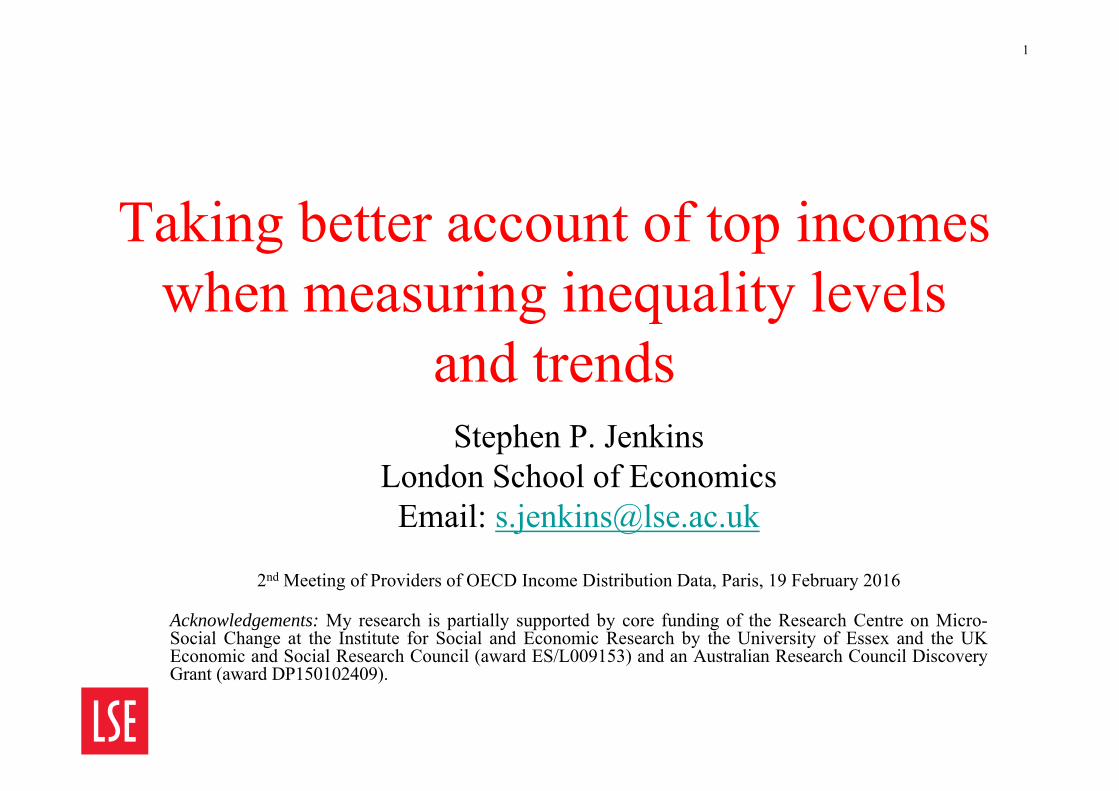
Two main sources of inequality data

Household surveys• E.g. OECD IDD

Income tax returns• E.g. World Top Incomes

Database (WTID) project

3

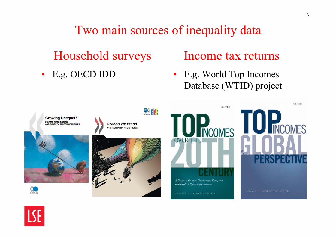
Surveys and tax return data provide different estimates of inequality trends: UK

Notes: The Gini and p90/p10 measures are based on household survey data using the same definitions as employed by the UK’s official income distribution statistics (source: authors’ derivations from the spreadsheet accompanying Belfield et al. 2015). The top 1% share measure is based on tax return data (source: authors’ derivations from Alvaredo et al. 2015). The data sources and income definitions that each series employs are discussed further in Section 2 of Burkhauser et al. (2016)

4

60

80

100

120

140

160

180

Ineq

ualit

y (in

dexe

d 19

62 =

100

)

1960 1965 1970 1975 1980 1985 1990 1995 2000 2005 2010 2015

Gini p90/p10Share top 1%

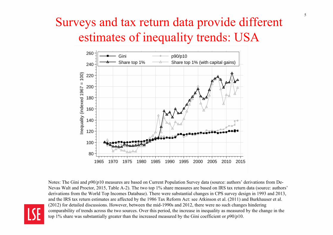
Surveys and tax return data provide different estimates of inequality trends: USA

Notes: The Gini and p90/p10 measures are based on Current Population Survey data (source: authors’ derivations from De-Nevas Walt and Proctor, 2015, Table A-2). The two top 1% share measures are based on IRS tax return data (source: authors’ derivations from the World Top Incomes Database). There were substantial changes in CPS survey design in 1993 and 2013, and the IRS tax return estimates are affected by the 1986 Tax Reform Act: see Atkinson et al. (2011) and Burkhauser et al. (2012) for detailed discussions. However, between the mid-1990s and 2012, there were no such changes hindering comparability of trends across the two sources. Over this period, the increase in inequality as measured by the change in thetop 1% share was substantially greater than the increased measured by the Gini coefficient or p90/p10.

5

80

100

120

140

160

180

200

220

240

260

Ineq

ualit

y (in

dexe

d 19

67 =

100

)

1965 1970 1975 1980 1985 1990 1995 2000 2005 2010 2015

Gini p90/p10Share top 1% Share top 1% (with capital gains)

The Problem

Under-coverage of top incomes in household surveys

6

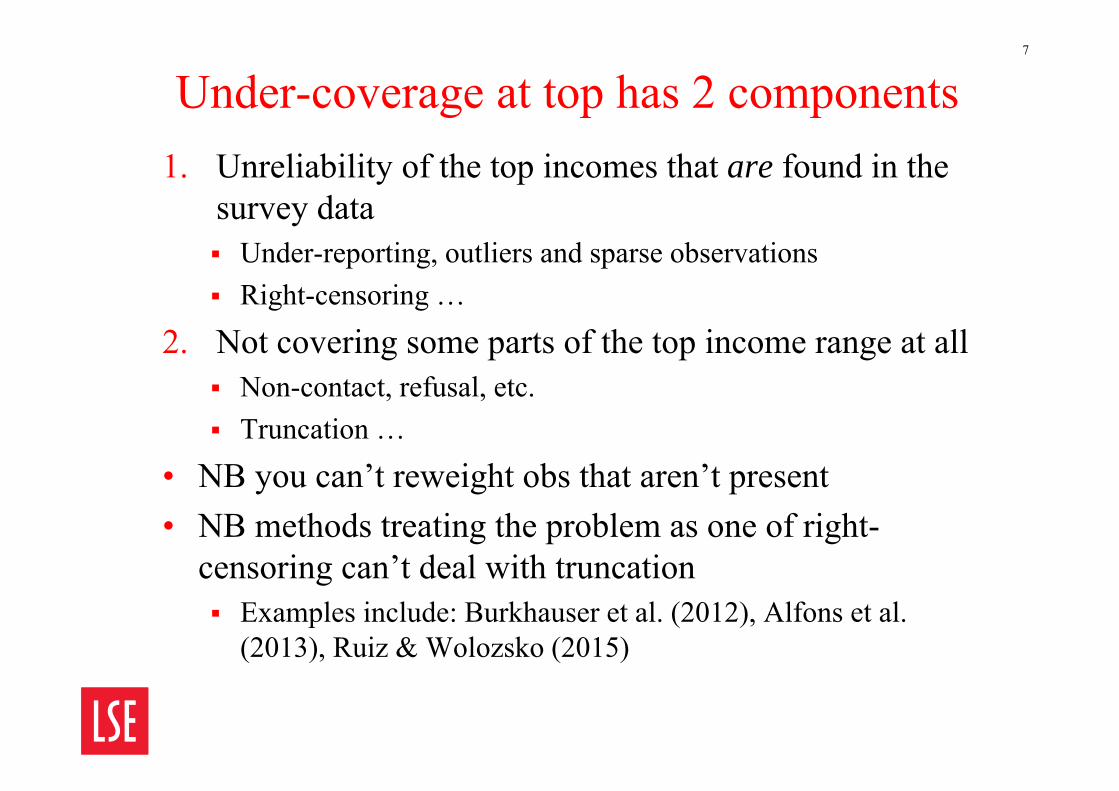
Under-coverage at top has 2 components1. Unreliability of the top incomes that are found in the

survey data Under-reporting, outliers and sparse observations Right-censoring …

2. Not covering some parts of the top income range at all Non-contact, refusal, etc. Truncation …

• NB you can’t reweight obs that aren’t present• NB methods treating the problem as one of right-

censoring can’t deal with truncation Examples include: Burkhauser et al. (2012), Alfons et al.

(2013), Ruiz & Wolozsko (2015)

7

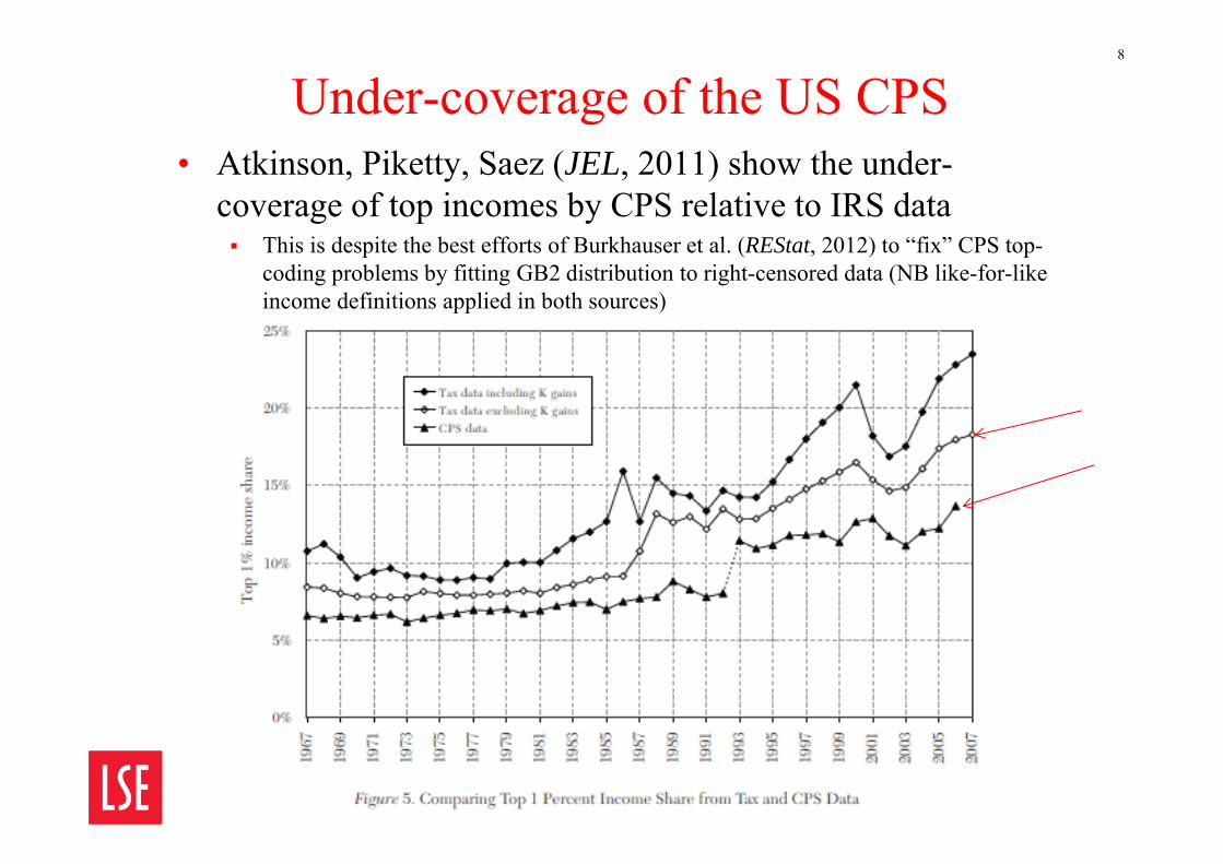
Under-coverage of the US CPS• Atkinson, Piketty, Saez (JEL, 2011) show the under-

coverage of top incomes by CPS relative to IRS data This is despite the best efforts of Burkhauser et al. (REStat, 2012) to “fix” CPS top-

coding problems by fitting GB2 distribution to right-censored data (NB like-for-like income definitions applied in both sources)

8

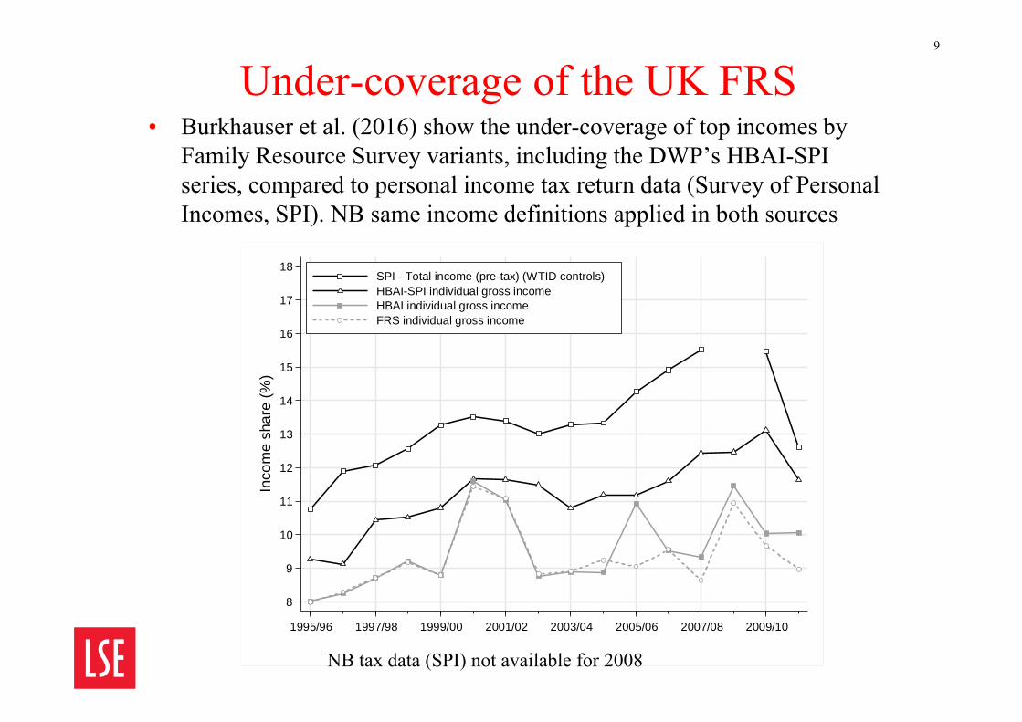
Under-coverage of the UK FRS• Burkhauser et al. (2016) show the under-coverage of top incomes by

Family Resource Survey variants, including the DWP’s HBAI-SPI series, compared to personal income tax return data (Survey of Personal Incomes, SPI). NB same income definitions applied in both sources

9

8

9

10

11

12

13

14

15

16

17

18In

com

e sh

are

(%)

1995/96 1997/98 1999/00 2001/02 2003/04 2005/06 2007/08 2009/10

SPI - Total income (pre-tax) (WTID controls)HBAI-SPI individual gross incomeHBAI individual gross incomeFRS individual gross income

NB tax data (SPI) not available for 2008

Solutions

Two approaches to addressing under-coverage at the top

10

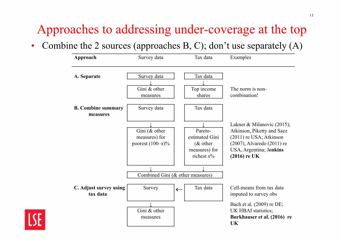
Approaches to addressing under-coverage at the top• Combine the 2 sources (approaches B, C); don’t use separately (A)

11

Approach Survey data Tax data Examples

A. Separate Survey data Tax data↓ ↓

Gini & other measures

Top income shares

The norm is non-combination!

B. Combine summary measures

Survey data Tax data

↓ ↓ Lakner & Milanovic (2015);Gini (& other measures) for

poorest (100–x)%

Pareto-estimated Gini

(& other measures) for

richest x%

Atkinson, Piketty and Saez(2011) re USA; Atkinson (2007), Alvaredo (2011) re USA, Argentina; Jenkins(2016) re UK

↓ ↓Combined Gini (& other measures)

C. Adjust survey using tax data

Survey Tax data Cell-means from tax data imputed to survey obs

↓ Bach et al. (2009) re DE;Gini & other

measuresUK HBAI statistics;Burkhauser et al. (2016) re UK

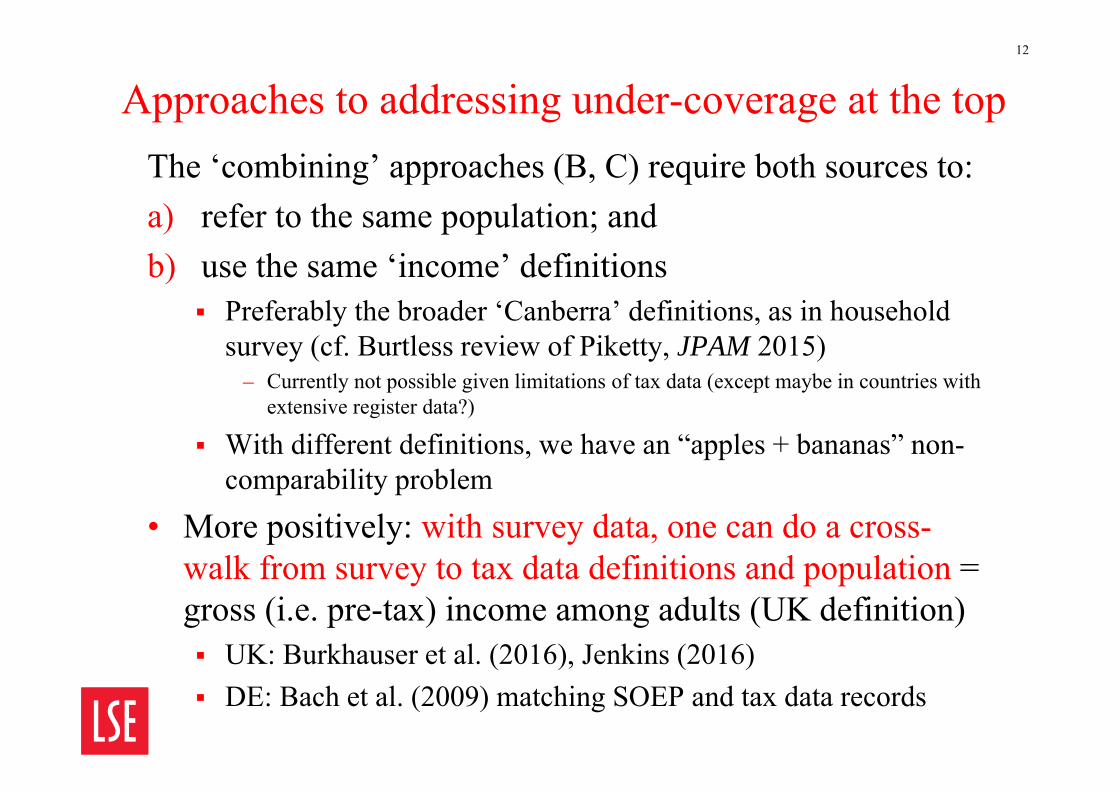
Approaches to addressing under-coverage at the topThe ‘combining’ approaches (B, C) require both sources to:a) refer to the same population; and b) use the same ‘income’ definitions

Preferably the broader ‘Canberra’ definitions, as in household survey (cf. Burtless review of Piketty, JPAM 2015)

– Currently not possible given limitations of tax data (except maybe in countries with extensive register data?)

With different definitions, we have an “apples + bananas” non-comparability problem

• More positively: with survey data, one can do a cross-walk from survey to tax data definitions and population = gross (i.e. pre-tax) income among adults (UK definition) UK: Burkhauser et al. (2016), Jenkins (2016) DE: Bach et al. (2009) matching SOEP and tax data records

12

Approach B: combining estimates

Estimate inequality and mean for top incomes (tax data) and for non-top incomes (survey data), and then derive a combined

inequality estimate for all incomes

13

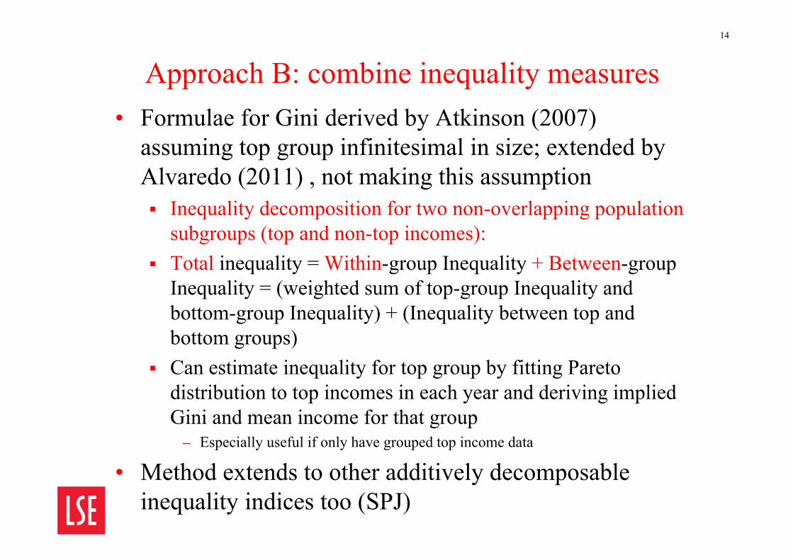
Approach B: combine inequality measures• Formulae for Gini derived by Atkinson (2007)

assuming top group infinitesimal in size; extended by Alvaredo (2011) , not making this assumption Inequality decomposition for two non-overlapping population

subgroups (top and non-top incomes): Total inequality = Within-group Inequality + Between-group

Inequality = (weighted sum of top-group Inequality and bottom-group Inequality) + (Inequality between top and bottom groups)

Can estimate inequality for top group by fitting Pareto distribution to top incomes in each year and deriving implied Gini and mean income for that group

– Especially useful if only have grouped top income data

• Method extends to other additively decomposable inequality indices too (SPJ)

14

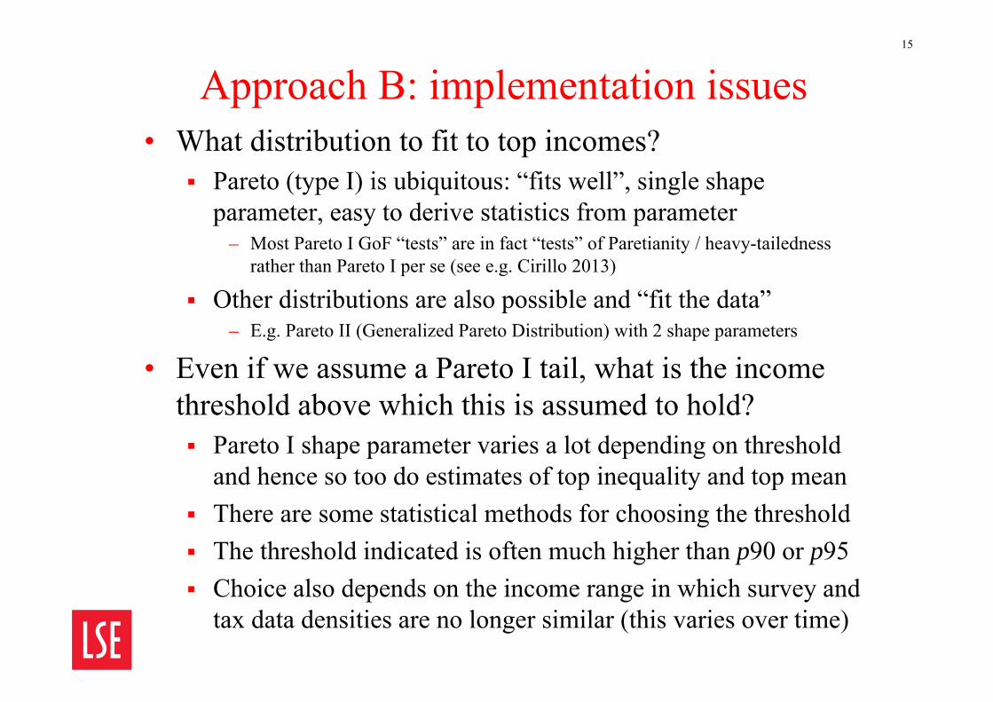
Approach B: implementation issues• What distribution to fit to top incomes?

Pareto (type I) is ubiquitous: “fits well”, single shape parameter, easy to derive statistics from parameter

– Most Pareto I GoF “tests” are in fact “tests” of Paretianity / heavy-tailednessrather than Pareto I per se (see e.g. Cirillo 2013)

Other distributions are also possible and “fit the data”– E.g. Pareto II (Generalized Pareto Distribution) with 2 shape parameters

• Even if we assume a Pareto I tail, what is the income threshold above which this is assumed to hold? Pareto I shape parameter varies a lot depending on threshold

and hence so too do estimates of top inequality and top mean There are some statistical methods for choosing the threshold The threshold indicated is often much higher than p90 or p95 Choice also depends on the income range in which survey and

tax data densities are no longer similar (this varies over time)

15

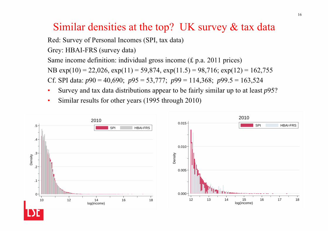
Similar densities at the top? UK survey & tax dataRed: Survey of Personal Incomes (SPI, tax data)Grey: HBAI-FRS (survey data)Same income definition: individual gross income (£ p.a. 2011 prices)NB exp(10) = 22,026, exp(11) = 59,874, exp(11.5) = 98,716; exp(12) = 162,755Cf. SPI data: p90 = 40,690; p95 = 53,777; p99 = 114,368; p99.5 = 163,524• Survey and tax data distributions appear to be fairly similar up to at least p95?• Similar results for other years (1995 through 2010)

16

0.000

0.005

0.010

0.015

Den

sity

12 13 14 15 16 17 18log(income)

SPI HBAI-FRS

2010

0

.1

.2

.3

.4

.5

Den

sity

10 12 14 16 18log(income)

SPI HBAI-FRS

2010

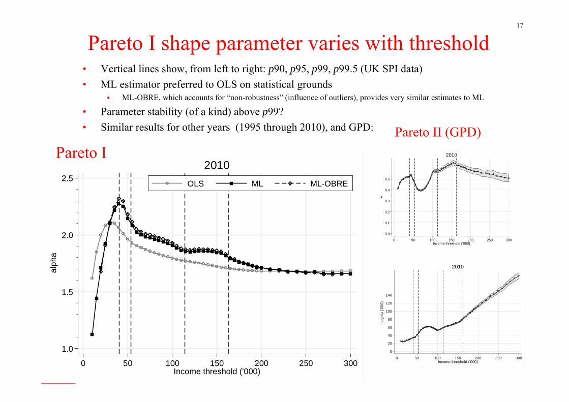
Pareto I shape parameter varies with threshold• Vertical lines show, from left to right: p90, p95, p99, p99.5 (UK SPI data)• ML estimator preferred to OLS on statistical grounds

ML-OBRE, which accounts for “non-robustness” (influence of outliers), provides very similar estimates to ML

• Parameter stability (of a kind) above p99?• Similar results for other years (1995 through 2010), and GPD:

17

1.0

1.5

2.0

2.5

alph

a

0 50 100 150 200 250 300Income threshold ('000)

OLS ML ML-OBRE

2010

0.0

0.1

0.2

0.3

0.4

0.5

xi

0 50 100 150 200 250 300Income threshold ('000)

2010

0

20

40

60

80

100

120

140

sigm

a ('0

00)

0 50 100 150 200 250 300Income threshold ('000)

2010

Pareto IPareto II (GPD)

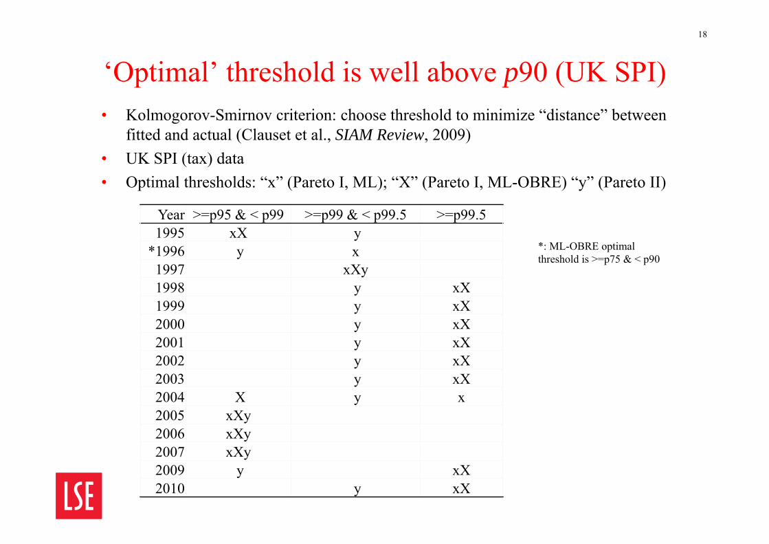
‘Optimal’ threshold is well above p90 (UK SPI)18

• Kolmogorov-Smirnov criterion: choose threshold to minimize “distance” between fitted and actual (Clauset et al., SIAM Review, 2009)

• UK SPI (tax) data• Optimal thresholds: “x” (Pareto I, ML); “X” (Pareto I, ML-OBRE) “y” (Pareto II)

Year >=p95 & < p99 >=p99 & < p99.5 >=p99.51995 xX y

*1996 y x1997 xXy1998 y xX1999 y xX2000 y xX2001 y xX2002 y xX2003 y xX2004 X y x2005 xXy2006 xXy2007 xXy2009 y xX2010 y xX

*: ML-OBRE optimalthreshold is >=p75 & < p90

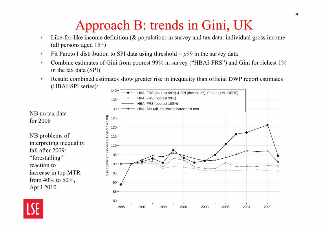
Approach B: trends in Gini, UK• Like-for-like income definition (& population) in survey and tax data: individual gross income

(all persons aged 15+)• Fit Pareto I distribution to SPI data using threshold = p99 in the survey data• Combine estimates of Gini from poorest 99% in survey (“HBAI-FRS”) and Gini for richest 1%

in the tax data (SPI)• Result: combined estimates show greater rise in inequality than official DWP report estimates

(HBAI-SPI series):

19

80

85

90

95

100

105

110

115

120

125

130

135

140

Gin

i coe

ffici

ent (

inde

xed

1996

-97

= 10

0)

1995 1997 1999 2001 2003 2005 2007 2009

HBAI-FRS (poorest 99%) & SPI (richest 1%), Pareto I (ML-OBRE)HBAI-FRS (poorest 99%)HBAI-FRS (poorest 100%)HBAI-SPI (all, equivalent household net)

NB no tax datafor 2008

NB problems ofinterpreting inequalityfall after 2009:“forestalling” reaction to increase in top MTRfrom 40% to 50%, April 2010

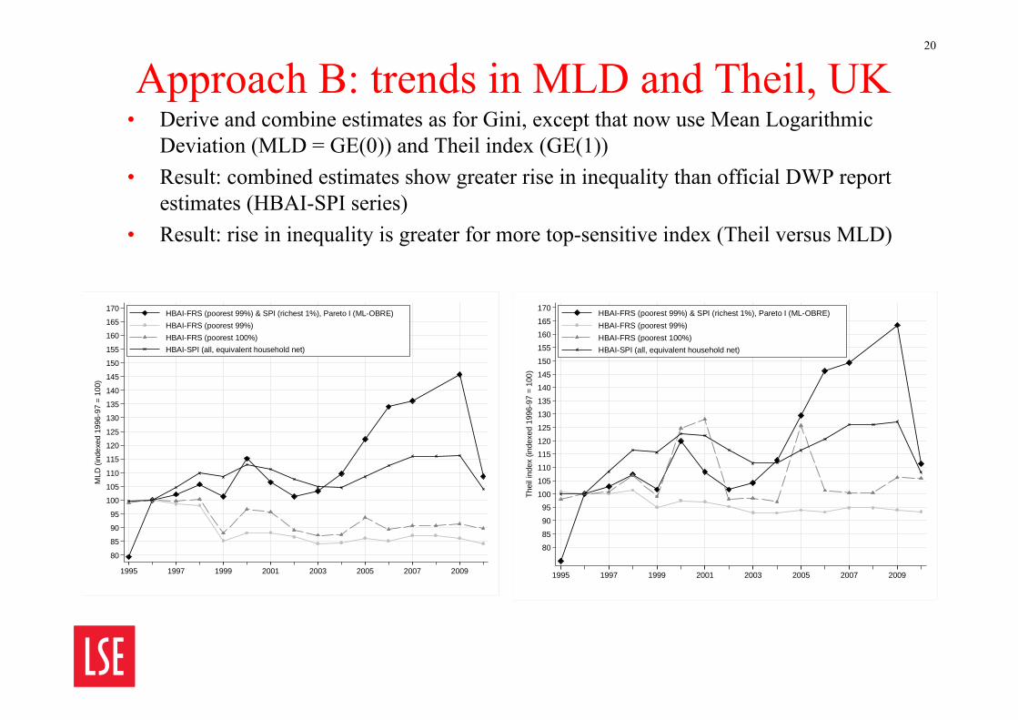
Approach B: trends in MLD and Theil, UK• Derive and combine estimates as for Gini, except that now use Mean Logarithmic

Deviation (MLD = GE(0)) and Theil index (GE(1)) • Result: combined estimates show greater rise in inequality than official DWP report

estimates (HBAI-SPI series)• Result: rise in inequality is greater for more top-sensitive index (Theil versus MLD)

20

80

85

90

95

100

105

110

115

120

125

130

135

140

145

150

155

160

165

170

MLD

(ind

exed

199

6-97

= 1

00)

1995 1997 1999 2001 2003 2005 2007 2009

HBAI-FRS (poorest 99%) & SPI (richest 1%), Pareto I (ML-OBRE)HBAI-FRS (poorest 99%)HBAI-FRS (poorest 100%)HBAI-SPI (all, equivalent household net)

80

85

90

95100

105

110

115120

125

130

135

140145

150

155

160165

170

Thei

l ind

ex (i

ndex

ed 1

996-

97 =

100

)

1995 1997 1999 2001 2003 2005 2007 2009

HBAI-FRS (poorest 99%) & SPI (richest 1%), Pareto I (ML-OBRE)HBAI-FRS (poorest 99%)HBAI-FRS (poorest 100%)HBAI-SPI (all, equivalent household net)

Approach C: combining data

Use cell-mean imputations from tax data to replace top income obs in the

survey data, and then calculate inequality index from combined data

21

Approach C: UK SPI-adjustmentThe data used to calculate UK official “HBAI” estimates contain an ‘SPI-adjustment’ to “improve the quality of data on very high incomes and combat spurious volatility” (DSS Working Group, 1996: 23)1. Replacement of a small number of “very rich” FRS respondents’

individual gross incomes in year t by cell-mean imputations ‘projected’ from tax data (SPI) for year t–1 Distinction between pensioner and non-pensioner households. In mid-1990s, about

0.2% of (weighted) individuals had incomes SPI-adjusted; proportion increased steadily in the early 2000s; since 2008/09, fixed at c. 0.5 %

Benefit-unit and household incomes recalculated post-imputation

2. Recalibration of FRS weights to better gross-up to population (shift in weight towards top income holders)

• Introduced first in 1992 (after DSS ‘Stocktaking’ report 1991), when HBAI used Family Expenditure Survey data, and originally imputed tax/benefit unit income from SPI, later changing to imputing individual incomes reflecting the change to individual taxation from 1990 and thence SPI data collection

22

C: Burkhauser et al. (2016) “SPI2” adjustment• More extensive systematic application of DWP approach• Make adjustments in the HBAI data in order to obtain top

1% income shares (and top 0.5% and 0.1% income shares) that are fully consistent with the WTID benchmark

• Then explore distributional trends, cross-walking between tax data and survey data definitions, and exploiting survey ‘flexibility’ (change receipt unit definition; summary index)

“SPI2” adjustment:1. Rank individuals in the SPI according to total pre-tax income (TI)2. Group individuals, with each group the size of 1/1000th of the total adult population (as

given by WTID control totals) and group mean income3. Repeat steps 1 to 2 with the HBAI data using our derived measure of (non-SPI’d)

individual gross income4. Replace individual income in the HBAI by the mean income of the same group in the

SPI for the 10 top income groups (i.e. the top 1 per cent)5. Total pre-tax income for the top 1 per cent is now the same in the HBAI and in the

WTID/SPI

23

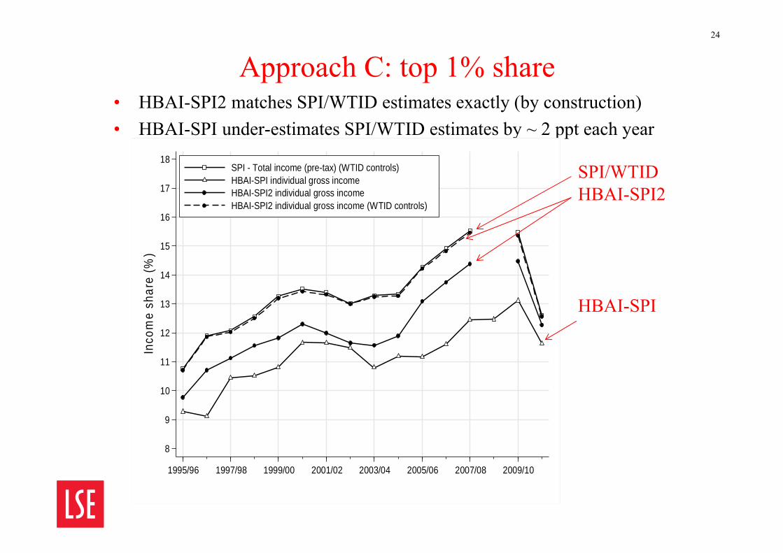
Approach C: top 1% share• HBAI-SPI2 matches SPI/WTID estimates exactly (by construction)• HBAI-SPI under-estimates SPI/WTID estimates by ~ 2 ppt each year

24

SPI/WTIDHBAI-SPI2

HBAI-SPI

8

9

10

11

12

13

14

15

16

17

18In

com

e sh

are

(%)

1995/96 1997/98 1999/00 2001/02 2003/04 2005/06 2007/08 2009/10

SPI - Total income (pre-tax) (WTID controls)HBAI-SPI individual gross incomeHBAI-SPI2 individual gross incomeHBAI-SPI2 individual gross income (WTID controls)

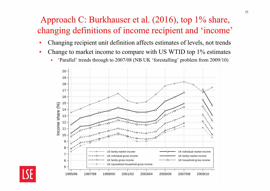
Approach C: Burkhauser et al. (2016), top 1% share, changing definitions of income recipient and ‘income’• Changing recipient unit definition affects estimates of levels, not trends• Change to market income to compare with US WTID top 1% estimates

‘Parallel’ trends through to 2007/08 (NB UK ‘forestalling’ problem from 2009/10)

25

5

6

7

8

9

10

11

12

13

14

15

16

17

18

19

20

Inco

me

shar

e (%

)

1995/96 1997/98 1999/00 2001/02 2003/04 2005/06 2007/08 2009/10

US family market income UK individual market income

UK individual gross income UK family market income

UK family gross income UK household gross incomeUK equivalised household gross income

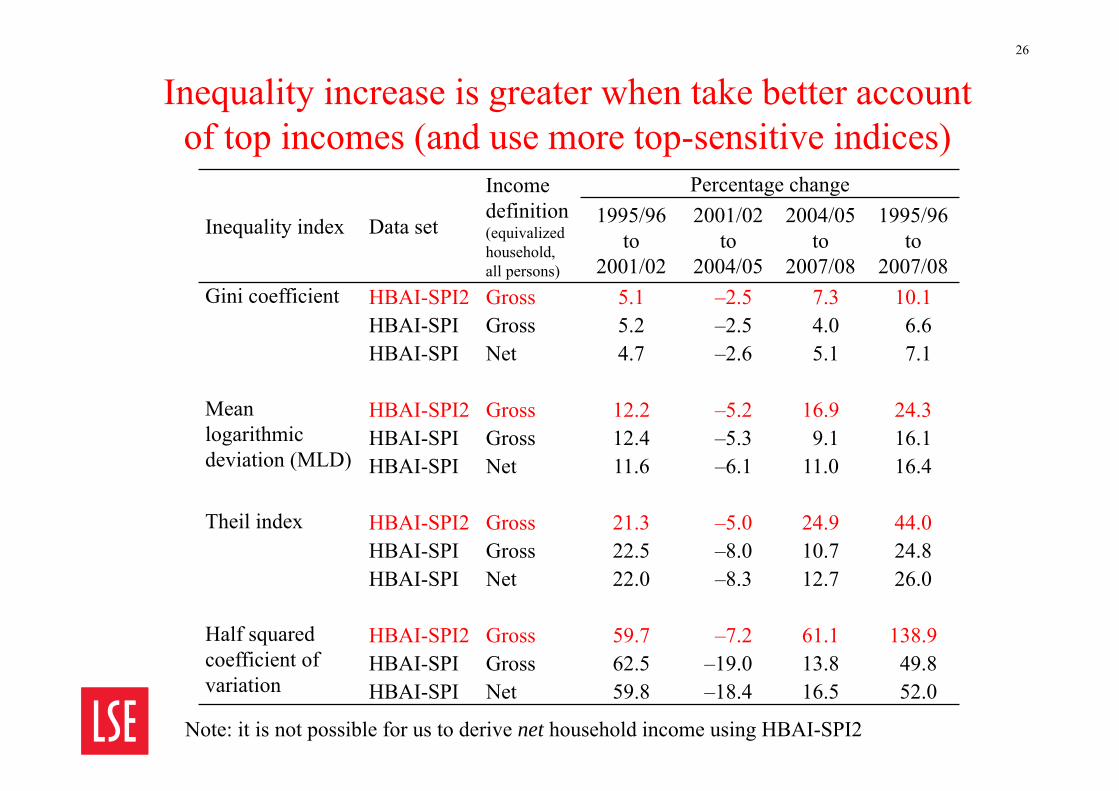
Inequality increase is greater when take better account of top incomes (and use more top-sensitive indices)

Inequality index Data set

Income definition (equivalizedhousehold, all persons)

Percentage change1995/96

to 2001/02

2001/02 to

2004/05

2004/05 to

2007/08

1995/96 to

2007/08Gini coefficient HBAI-SPI2 Gross 5.1 –2.5 7.3 10.1

HBAI-SPI Gross 5.2 –2.5 4.0 6.6HBAI-SPI Net 4.7 –2.6 5.1 7.1

Mean logarithmic deviation (MLD)

HBAI-SPI2 Gross 12.2 –5.2 16.9 24.3HBAI-SPI Gross 12.4 –5.3 9.1 16.1HBAI-SPI Net 11.6 –6.1 11.0 16.4

Theil index HBAI-SPI2 Gross 21.3 –5.0 24.9 44.0HBAI-SPI Gross 22.5 –8.0 10.7 24.8HBAI-SPI Net 22.0 –8.3 12.7 26.0

Half squared coefficient of variation

HBAI-SPI2 Gross 59.7 –7.2 61.1 138.9HBAI-SPI Gross 62.5 –19.0 13.8 49.8HBAI-SPI Net 59.8 –18.4 16.5 52.0

26

Note: it is not possible for us to derive net household income using HBAI-SPI2

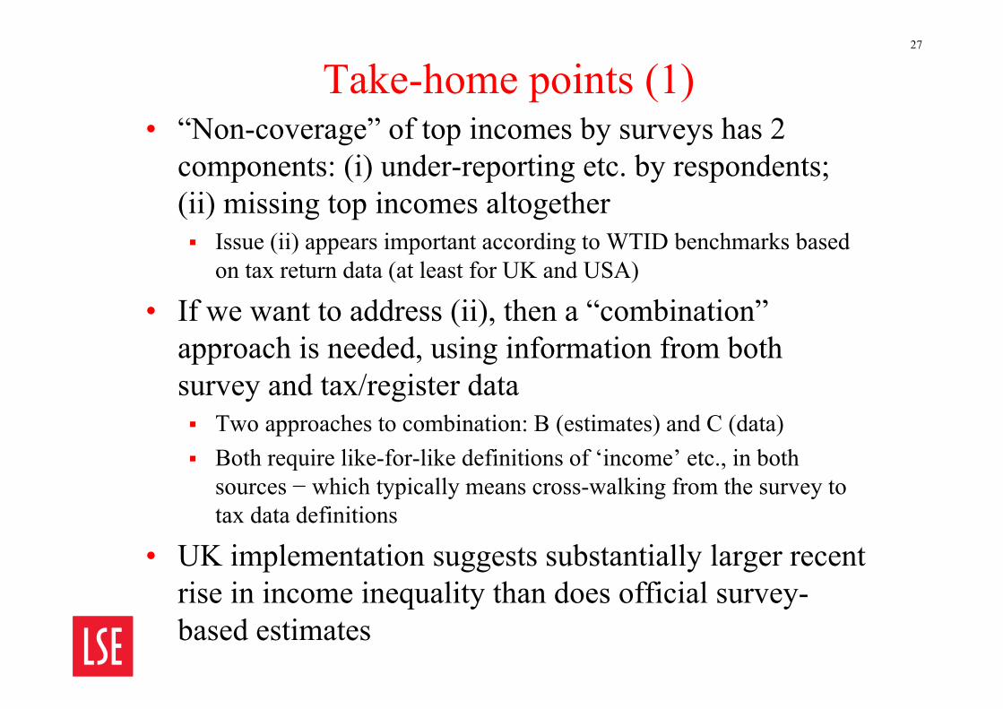
Take-home points (1)• “Non-coverage” of top incomes by surveys has 2

components: (i) under-reporting etc. by respondents; (ii) missing top incomes altogether Issue (ii) appears important according to WTID benchmarks based

on tax return data (at least for UK and USA)

• If we want to address (ii), then a “combination” approach is needed, using information from both survey and tax/register data Two approaches to combination: B (estimates) and C (data) Both require like-for-like definitions of ‘income’ etc., in both

sources − which typically means cross-walking from the survey to tax data definitions

• UK implementation suggests substantially larger recent rise in income inequality than does official survey-based estimates

27

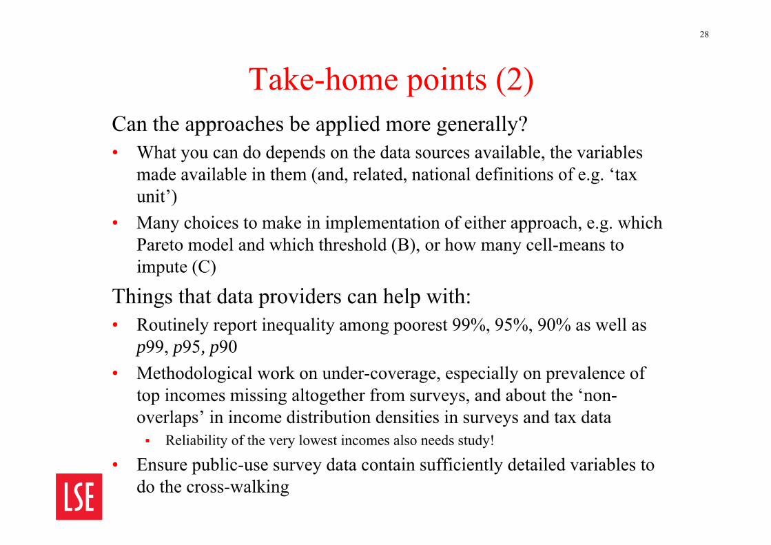
Take-home points (2)Can the approaches be applied more generally?• What you can do depends on the data sources available, the variables

made available in them (and, related, national definitions of e.g. ‘tax unit’)

• Many choices to make in implementation of either approach, e.g. which Pareto model and which threshold (B), or how many cell-means to impute (C)

Things that data providers can help with:• Routinely report inequality among poorest 99%, 95%, 90% as well as

p99, p95, p90• Methodological work on under-coverage, especially on prevalence of

top incomes missing altogether from surveys, and about the ‘non-overlaps’ in income distribution densities in surveys and tax data Reliability of the very lowest incomes also needs study!

• Ensure public-use survey data contain sufficiently detailed variables to do the cross-walking

28

Selected references• Jenkins, S. P. (in preparation). ‘Pareto distributions, top incomes, and recent trends in UK income

inequality’, invited plenary lecture at Conference on the ‘Dynamics of Inequalities and their Perceptions’, Aix-Marseilles University, Marseilles, 26–27 May 2016

• Burkhauser, R. V., Hérault, N., Jenkins, S. P., and Wilkins, R. (2016), ‘What has been happening to UK income inequality since the mid-1990s? Answers from reconciled and combined household survey and tax return data’, NBER Working Paper w21991 (http://www.nber.org/papers/w21991), IZA Discussion Paper No. 9718 (http://ftp.iza.org/dp9718.pdf), ISER Working Paper 2016-03 (https://www.iser.essex.ac.uk/research/publications/working-papers/iser/2016-03).

• Alfons, A., Templ, M. and Filzmoser, P. (2013). Robust estimation of economic indicators from survey samples based on Pareto tail modelling. Journal of the Royal Statistical Society, Series C, 62 (2), 271286.

• Atkinson, A. B., Piketty, T., and Saez, E. (2011). Top incomes in the long run of history. Journal of Economic Literature, 49 (1), 371.

• Bach, S., Corneo, G. and Steiner, V. (2009). From bottom to top. The entire income distribution in Germany, 19922003. Review of Income and Wealth, 55 (2), 303330.

• Burkhauser, R.V., Feng, S., Jenkins, S. P., and Larrimore, J. (2012). Recent trends in top income shares in the USA: reconciling estimates from March CPS and IRS tax return data, Review of Economics and Statistics, 94 (2), 371388.

• Cirillo, P. (2013). Are your data really Pareto distributed? Physica A, 392, 59475962 • Clauset, A., Shaliza, C. R., and Newman, M. E. J. (2009). Power-law distributions in empirical data.

SIAM Review, 51 (4), 661703• Department for Work and Pensions (2015). Households Below Average Income An Analysis of the

Income Distribution 1994/95 – 2013/14. London: Department for Work and Pensions • Ruiz, N. and Woloszko, N. (2015). What do household surveys suggest about the top 1% incomes and

inequality in OECD countries? OECD Economics Department Working Papers, No. 1265, http://dx.doi.org/10.1787/5jrs556f36zt-en

29