Takeo Ohsawa L² Approaches in Several Complex Variables
267
Springer Monographs in Mathematics Takeo Ohsawa L ² Approaches in Several Complex Variables Towards the Oka–Cartan Theory with Precise Bounds Second Edition
Transcript of Takeo Ohsawa L² Approaches in Several Complex Variables
Springer Monographs in Mathematics
Takeo Ohsawa
L² Approaches in Several Complex VariablesTowards the Oka–Cartan Theory with Precise Bounds
Second Edition

Springer Monographs in Mathematics
Editors-in-Chief
Isabelle Gallagher, Paris, FranceMinhyong Kim, Oxford, UK
Series Editors
Sheldon Axler, San Francisco, USAMark Braverman, Princeton, USAMaria Chudnovsky, Princeton, USATadahisa Funaki, Tokyo, JapanSinan C. Güntürk, New York, USAClaude Le Bris, Marne la Vallée, FrancePascal Massart, Orsay, FranceAlberto Pinto, Porto, PortugalGabriella Pinzari, Napoli, ItalyKen Ribet, Berkeley, USARené Schilling, Dresden, GermanyPanagiotis Souganidis, Chicago, USAEndre Süli, Oxford, UKShmuel Weinberger, Chicago, USABoris Zilber, Oxford, UK

This series publishes advanced monographs giving well-written presentations ofthe “state-of-the-art” in fields of mathematical research that have acquired thematurity needed for such a treatment. They are sufficiently self-contained to beaccessible to more than just the intimate specialists of the subject, and sufficientlycomprehensive to remain valuable references for many years. Besides the currentstate of knowledge in its field, an SMM volume should ideally describe its relevanceto and interaction with neighbouring fields of mathematics, and give pointers tofuture directions of research.
More information about this series at http://www.springer.com/series/3733
Takeo Ohsawa
L2 Approaches in SeveralComplex VariablesTowards the Oka–Cartan Theory with PreciseBounds
Second Edition
123

Takeo OhsawaProfessor EmeritusNagoya UniversityNagoya, Japan
ISSN 1439-7382 ISSN 2196-9922 (electronic)Springer Monographs in MathematicsISBN 978-4-431-56851-3 ISBN 978-4-431-56852-0 (eBook)https://doi.org/10.1007/978-4-431-56852-0
Library of Congress Control Number: 2018959147
© Springer Japan KK, part of Springer Nature 2015, 2018This work is subject to copyright. All rights are reserved by the Publisher, whether the whole or part ofthe material is concerned, specifically the rights of translation, reprinting, reuse of illustrations, recitation,broadcasting, reproduction on microfilms or in any other physical way, and transmission or informationstorage and retrieval, electronic adaptation, computer software, or by similar or dissimilar methodologynow known or hereafter developed.The use of general descriptive names, registered names, trademarks, service marks, etc. in this publicationdoes not imply, even in the absence of a specific statement, that such names are exempt from the relevantprotective laws and regulations and therefore free for general use.The publisher, the authors and the editors are safe to assume that the advice and information in this bookare believed to be true and accurate at the date of publication. Neither the publisher nor the authors orthe editors give a warranty, express or implied, with respect to the material contained herein or for anyerrors or omissions that may have been made. The publisher remains neutral with regard to jurisdictionalclaims in published maps and institutional affiliations.
This Springer imprint is published by the registered company Springer Japan KK part of Springer Nature.The registered company address is: Shiroyama Trust Tower, 4-3-1 Toranomon, Minato-ku, Tokyo105-6005, Japan
Preface
As in the study of complex analysis of one variable, the general theory of severalcomplex variables has manifold aspects. First, it provides a firm ground forsystematic studies of special functions such as elliptic functions, theta functions,and modular functions. The general theory plays a role of confirming the existenceand uniqueness of functions with prescribed zeros and poles. Another aspect is togive an insight into the connection between two different fields of mathematicsby understanding how the tools work. The theory of sheaves bridged analysis andtopology in such a way. In the construction of this basic theory of several complexvariables, a particularly important contribution was made by two mathematicians,Kiyoshi Oka (1901–1978) and Henri Cartan (1904–2008). The theory of Oka andCartan is condensed in a statement that the first cohomology of coherent analyticsheaves over Cn is zero. On the other hand, the method of PDE (partial differentialequations) had turned out to be essential in the existence of conformal mappings. Bythis approach, the function theory on Riemann surfaces as one-dimensional complexmanifolds was explored by H. Weyl. Weyl’s method was developed on manifolds ofhigher dimension by K. Kodaira who generalized Riemann’s condition for Abelianvarieties by establishing a differential geometric characterization of nonsingularprojective algebraic varieties. This PDE method, based on the L2 estimates forthe ∂-operator, was generalized by J. Kohn, L. Hörmander, A. Andreotti, andE. Vesentini. As a result, it enabled us to see the results of Oka and Cartan ina much higher resolution. In particular, based on such a refinement, existencetheorems for holomorphic functions with L2 growth conditions have been obtainedby Hörmander, H. Skoda, and others. The purpose of the present monograph isto report on some of the recent results in several complex variables obtained bythe L2 method which can be regarded as a continuation of these works. Amongvarious topics including complex geometry, the Bergman kernel, and holomorphicfoliations, a special emphasis is put on the extension theorems and its applications.In this topic, highlighted are the recent developments after the solution of a long-standing open question of N. Suita. It is an inequality between the Bergman kerneland the logarithmic capacity on Riemann surfaces, which was first proved byZ. Błocki for plane domains. Q. Guan and X.-Y. Zhou proved generalized variants
v

vi Preface
and characterized those surfaces on which the inequality is strict. Their work gavethe author a decisive impetus to start writing a survey to cover these remarkableachievements. As a result, he could find an alternate proof of the inequality,based on hyperbolic geometry, which is presented in Chap. 3. However, the readersare recommended to have a glance at Chap. 4 first, where the questions on theBergman kernels are described more systematically. (The author started to writethe monograph from Chap. 4.) Since there have been a lot of subsequent progressconcerning the materials in Chaps. 3 and 4 during the preparation of the manuscript,it soon became beyond the author’s ability to give a satisfactory account of the wholedevelopment. So he will be happy to have a chance in the future to revise and enlargethis rather brief monograph.
Nagoya, Japan Takeo OhsawaMarch 2015
Preface to the Second Edition
Thanks to the goodwill of the publisher, the revision and enlargement have beenrealized. What made this edition possible was the recent remarkable activity afterBłocki’s solution of Suita’s conjecture for plane domains. Among many corrections,the most important one is the replacement of an erroneous proof of Theorem 3.2 bythe present one which is hopefully correct. The author is very grateful to ShigeharuTakayama for pointing out the mistake. Additions have been made to focus onthe results which appeared in the past 3 years. Some of them are in Sect. 4.4.5“Berndtsson–Lempert Theory and Beyond” and in the section “A History of LeviFlat Hypersurfaces” in 5.3. Besides these, each chapter has been supplemented bya section titled “Notes and Remarks,” in which the author also tried to enhance thedepth feeling of complex analysis and convey the atmosphere of several complexvariables similar to searching for extraterrestrial intelligence since Hartogs and Oka.
Nagoya, Japan Takeo OhsawaApril 2018
vii

Contents
1 Basic Notions and Classical Results . . . . . . . . . . . . . . . . . . . . . . . . . . . . . . . . . . . . . . . . 11.1 Functions and Domains Over Cn . . . . . . . . . . . . . . . . . . . . . . . . . . . . . . . . . . . . . . . 2
1.1.1 Holomorphic Functions and Cauchy’s Formula . . . . . . . . . . . . . . . 21.1.2 Weierstrass Preparation Theorem . . . . . . . . . . . . . . . . . . . . . . . . . . . . . . 41.1.3 Domains of Holomorphy and Plurisubharmonic Functions . . 7
1.2 Complex Manifolds and Convexity Notions . . . . . . . . . . . . . . . . . . . . . . . . . . . 91.2.1 Complex Manifolds, Stein Manifolds and Holomorphic
Convexity . . . . . . . . . . . . . . . . . . . . . . . . . . . . . . . . . . . . . . . . . . . . . . . . . . . . . . . 101.2.2 Complex Exterior Derivatives and Levi Form. . . . . . . . . . . . . . . . . 141.2.3 Pseudoconvex Manifolds and Oka–Grauert Theory . . . . . . . . . . 16
1.3 Oka–Cartan Theory . . . . . . . . . . . . . . . . . . . . . . . . . . . . . . . . . . . . . . . . . . . . . . . . . . . . . 191.3.1 Sheaves and Cohomology . . . . . . . . . . . . . . . . . . . . . . . . . . . . . . . . . . . . . . 191.3.2 Coherent Sheaves, Complex Spaces, and Theorems A
and B . . . . . . . . . . . . . . . . . . . . . . . . . . . . . . . . . . . . . . . . . . . . . . . . . . . . . . . . . . . . 251.3.3 Coherence of Direct Images and a Theorem of
Andreotti and Grauert . . . . . . . . . . . . . . . . . . . . . . . . . . . . . . . . . . . . . . . . . . 301.4 ∂-Equations on Manifolds . . . . . . . . . . . . . . . . . . . . . . . . . . . . . . . . . . . . . . . . . . . . . . 31
1.4.1 Holomorphic Vector Bundles and ∂-Cohomology . . . . . . . . . . . . 321.4.2 Cohomology with Compact Support. . . . . . . . . . . . . . . . . . . . . . . . . . . 361.4.3 Serre’s Duality Theorem . . . . . . . . . . . . . . . . . . . . . . . . . . . . . . . . . . . . . . . 381.4.4 Fiber Metric and L2 Spaces . . . . . . . . . . . . . . . . . . . . . . . . . . . . . . . . . . . . 41
1.5 Notes and Remarks . . . . . . . . . . . . . . . . . . . . . . . . . . . . . . . . . . . . . . . . . . . . . . . . . . . . . 42References . . . . . . . . . . . . . . . . . . . . . . . . . . . . . . . . . . . . . . . . . . . . . . . . . . . . . . . . . . . . . . . . . . . . . 45
2 Analyzing the L2 ∂-Cohomology . . . . . . . . . . . . . . . . . . . . . . . . . . . . . . . . . . . . . . . . . . . 472.1 Orthogonal Decompositions in Hilbert Spaces . . . . . . . . . . . . . . . . . . . . . . . . 47
2.1.1 Basics on Closed Operators . . . . . . . . . . . . . . . . . . . . . . . . . . . . . . . . . . . . 472.1.2 Kodaira’s Decomposition Theorem and Hörmander’s
Lemma . . . . . . . . . . . . . . . . . . . . . . . . . . . . . . . . . . . . . . . . . . . . . . . . . . . . . . . . . . 482.1.3 Remarks on the Closedness . . . . . . . . . . . . . . . . . . . . . . . . . . . . . . . . . . . . 50
ix
x Contents
2.2 Vanishing Theorems . . . . . . . . . . . . . . . . . . . . . . . . . . . . . . . . . . . . . . . . . . . . . . . . . . . . 512.2.1 Metrics and L2 ∂-Cohomology . . . . . . . . . . . . . . . . . . . . . . . . . . . . . . . . 512.2.2 Complete Metrics and Gaffney’s Theorem . . . . . . . . . . . . . . . . . . . . 542.2.3 Some Commutator Relations . . . . . . . . . . . . . . . . . . . . . . . . . . . . . . . . . . . 552.2.4 Positivity and L2 Estimates . . . . . . . . . . . . . . . . . . . . . . . . . . . . . . . . . . . . 582.2.5 L2 Vanishing Theorems on Complete Kähler Manifolds . . . . . 602.2.6 Pseudoconvex Cases . . . . . . . . . . . . . . . . . . . . . . . . . . . . . . . . . . . . . . . . . . . . 662.2.7 Sheaf Theoretic Interpretation . . . . . . . . . . . . . . . . . . . . . . . . . . . . . . . . . 672.2.8 Application to the Cohomology of Complex Spaces . . . . . . . . . 70
2.3 Finiteness Theorems . . . . . . . . . . . . . . . . . . . . . . . . . . . . . . . . . . . . . . . . . . . . . . . . . . . . 772.3.1 L2 Finiteness Theorems on Complete Manifolds . . . . . . . . . . . . . 772.3.2 Approximation and Isomorphism Theorems . . . . . . . . . . . . . . . . . . 79
2.4 Notes on Metrics and Pseudoconvexity . . . . . . . . . . . . . . . . . . . . . . . . . . . . . . . 882.4.1 Pseudoconvex Manifolds with Positive Line Bundles . . . . . . . . 892.4.2 Geometry of the Boundaries of Complete Kähler Domains . . 912.4.3 Curvature and Pseudoconvexity . . . . . . . . . . . . . . . . . . . . . . . . . . . . . . . . 942.4.4 Miscellanea on Locally Pseudoconvex Domains. . . . . . . . . . . . . . 95
2.5 Notes and Remarks . . . . . . . . . . . . . . . . . . . . . . . . . . . . . . . . . . . . . . . . . . . . . . . . . . . . . 99References . . . . . . . . . . . . . . . . . . . . . . . . . . . . . . . . . . . . . . . . . . . . . . . . . . . . . . . . . . . . . . . . . . . . . 111
3 L2 Oka–Cartan Theory . . . . . . . . . . . . . . . . . . . . . . . . . . . . . . . . . . . . . . . . . . . . . . . . . . . . . 1153.1 L2 Extension Theorems . . . . . . . . . . . . . . . . . . . . . . . . . . . . . . . . . . . . . . . . . . . . . . . . 115
3.1.1 Extension by the Twisted Nakano Identity . . . . . . . . . . . . . . . . . . . . 1153.1.2 L2 Extension Theorems on Complex Manifolds . . . . . . . . . . . . . . 1213.1.3 Application to Embeddings . . . . . . . . . . . . . . . . . . . . . . . . . . . . . . . . . . . . 1253.1.4 Application to Analytic Invariants . . . . . . . . . . . . . . . . . . . . . . . . . . . . . 127
3.2 L2 Division Theorems . . . . . . . . . . . . . . . . . . . . . . . . . . . . . . . . . . . . . . . . . . . . . . . . . . 1283.2.1 A Gauss–Codazzi-Type Formula . . . . . . . . . . . . . . . . . . . . . . . . . . . . . . 1293.2.2 Skoda’s Division Theorem . . . . . . . . . . . . . . . . . . . . . . . . . . . . . . . . . . . . . 1313.2.3 From Division to Extension . . . . . . . . . . . . . . . . . . . . . . . . . . . . . . . . . . . . 1353.2.4 Proof of a Precise L2 Division Theorem . . . . . . . . . . . . . . . . . . . . . . 138
3.3 L2 Approaches to Analytic Ideals . . . . . . . . . . . . . . . . . . . . . . . . . . . . . . . . . . . . . . 1403.3.1 Briançon–Skoda Theorem. . . . . . . . . . . . . . . . . . . . . . . . . . . . . . . . . . . . . . 1403.3.2 Nadel’s Coherence Theorem . . . . . . . . . . . . . . . . . . . . . . . . . . . . . . . . . . . 1423.3.3 Miscellanea on Multiplier Ideal Sheaves . . . . . . . . . . . . . . . . . . . . . . 142
3.4 Notes and Remarks . . . . . . . . . . . . . . . . . . . . . . . . . . . . . . . . . . . . . . . . . . . . . . . . . . . . . 153References . . . . . . . . . . . . . . . . . . . . . . . . . . . . . . . . . . . . . . . . . . . . . . . . . . . . . . . . . . . . . . . . . . . . . 161
4 Bergman Kernels . . . . . . . . . . . . . . . . . . . . . . . . . . . . . . . . . . . . . . . . . . . . . . . . . . . . . . . . . . . . . 1654.1 Bergman Kernel and Metric . . . . . . . . . . . . . . . . . . . . . . . . . . . . . . . . . . . . . . . . . . . . 165
4.1.1 Bergman Kernels . . . . . . . . . . . . . . . . . . . . . . . . . . . . . . . . . . . . . . . . . . . . . . . 1664.1.2 The Bergman Metric . . . . . . . . . . . . . . . . . . . . . . . . . . . . . . . . . . . . . . . . . . . . 169
4.2 The Boundary Behavior . . . . . . . . . . . . . . . . . . . . . . . . . . . . . . . . . . . . . . . . . . . . . . . . 1704.2.1 Localization Principle . . . . . . . . . . . . . . . . . . . . . . . . . . . . . . . . . . . . . . . . . . 1714.2.2 Bergman’s Conjecture and Hörmander’s Theorem . . . . . . . . . . . 172

Contents xi
4.2.3 Miscellanea on the Boundary Behavior . . . . . . . . . . . . . . . . . . . . . . . 1734.2.4 Comparison with a Capacity Function . . . . . . . . . . . . . . . . . . . . . . . . . 177
4.3 Sequences of Bergman Kernels . . . . . . . . . . . . . . . . . . . . . . . . . . . . . . . . . . . . . . . . 1814.3.1 Weighted Sequences of Bergman Kernels . . . . . . . . . . . . . . . . . . . . . 1814.3.2 Demailly’s Approximation Theorem . . . . . . . . . . . . . . . . . . . . . . . . . . 1824.3.3 Towering Bergman Kernels . . . . . . . . . . . . . . . . . . . . . . . . . . . . . . . . . . . . 183
4.4 Parameter Dependence. . . . . . . . . . . . . . . . . . . . . . . . . . . . . . . . . . . . . . . . . . . . . . . . . . 1844.4.1 Stability Theorems. . . . . . . . . . . . . . . . . . . . . . . . . . . . . . . . . . . . . . . . . . . . . . 1844.4.2 Maitani–Yamaguchi Theorem. . . . . . . . . . . . . . . . . . . . . . . . . . . . . . . . . . 1854.4.3 Berndtsson’s Method . . . . . . . . . . . . . . . . . . . . . . . . . . . . . . . . . . . . . . . . . . . 1884.4.4 Guan–Zhou Method . . . . . . . . . . . . . . . . . . . . . . . . . . . . . . . . . . . . . . . . . . . . 1904.4.5 Berndtsson–Lempert Theory and Beyond . . . . . . . . . . . . . . . . . . . . . 192
4.5 Notes and Remarks . . . . . . . . . . . . . . . . . . . . . . . . . . . . . . . . . . . . . . . . . . . . . . . . . . . . . 194References . . . . . . . . . . . . . . . . . . . . . . . . . . . . . . . . . . . . . . . . . . . . . . . . . . . . . . . . . . . . . . . . . . . . . 201
5 L2 Approaches to Holomorphic Foliations . . . . . . . . . . . . . . . . . . . . . . . . . . . . . . . . 2055.1 Holomorphic Foliation . . . . . . . . . . . . . . . . . . . . . . . . . . . . . . . . . . . . . . . . . . . . . . . . . . 205
5.1.1 Foliation and Its Normal Bundle . . . . . . . . . . . . . . . . . . . . . . . . . . . . . . . 2055.1.2 Holomorphic Foliations of Codimension One. . . . . . . . . . . . . . . . . 208
5.2 Applications of the L2 Method . . . . . . . . . . . . . . . . . . . . . . . . . . . . . . . . . . . . . . . . . 2125.2.1 Applications to Stable Sets . . . . . . . . . . . . . . . . . . . . . . . . . . . . . . . . . . . . . 2125.2.2 Hartogs-Type Extensions by L2 Method . . . . . . . . . . . . . . . . . . . . . . 217
5.3 A History of Levi Flat Hypersurfaces . . . . . . . . . . . . . . . . . . . . . . . . . . . . . . . . . . 2205.4 Levi Flat Hypersurfaces in Tori and Hopf Surfaces . . . . . . . . . . . . . . . . . . . 226
5.4.1 Lemmas on Distance Functions . . . . . . . . . . . . . . . . . . . . . . . . . . . . . . . . 2265.4.2 A Reduction Theorem in Tori . . . . . . . . . . . . . . . . . . . . . . . . . . . . . . . . . . 2295.4.3 Classification in Hopf Surfaces . . . . . . . . . . . . . . . . . . . . . . . . . . . . . . . . 231
5.5 Notes and Remarks . . . . . . . . . . . . . . . . . . . . . . . . . . . . . . . . . . . . . . . . . . . . . . . . . . . . . 234References . . . . . . . . . . . . . . . . . . . . . . . . . . . . . . . . . . . . . . . . . . . . . . . . . . . . . . . . . . . . . . . . . . . . . 235
Bibliography . . . . . . . . . . . . . . . . . . . . . . . . . . . . . . . . . . . . . . . . . . . . . . . . . . . . . . . . . . . . . . . . . . . . . . 239
Index . . . . . . . . . . . . . . . . . . . . . . . . . . . . . . . . . . . . . . . . . . . . . . . . . . . . . . . . . . . . . . . . . . . . . . . . . . . . . . . 255
Chapter 1Basic Notions and Classical Results
Abstract As a preliminary, basic properties of holomorphic functions and complexmanifolds are recalled. Beginning with the definitions and characterizations ofholomorphic functions, we shall give an overview of the classical theorems inseveral complex variables, restricting ourselves to extremely important ones for thediscussion in later chapters. Most of the materials presented here are contained inwell-written textbooks such as Gunning and Rossi (Analytic functions of severalcomplex variables. Prentice-Hall, Inc., Englewood Cliffs, 1965, pp xiv+317),Hörmander (An introduction to complex analysis in several variables, 3rd edn.North-Holland Mathematical Library, vol 7. North-Holland Publishing Co., Ams-terdam, 1990, pp xii+254), Wells (Differential analysis on complex manifolds, 3rdedn. With a new appendix by Oscar Garcia-Prada. Graduate texts in mathematics,vol 65. Springer, New York, 2008), Grauert and Remmert (Theory of Stein spaces.Translated from the German by Alan Huckleberry. Reprint of the 1979 translation.Classics in mathematics. Springer, Berlin, 2004, pp xxii+255; Coherent analyticsheaves. Grundlehren der Mathematischen Wissenschaften, vol 265. Springer,Berlin, 1984, pp xviii+249) and Noguchi (Analytic function theory of severalvariables—elements of Oka’s coherence, preprint) (see also Demailly, Analyticmethods in algebraic geometry. Surveys of modern mathematics, vol 1. InternationalPress, Somerville/Higher Education Press, Beijing, 2012, pp viii+231) and Ohsawa(Analysis of several complex variables. Translated from the Japanese by ShuGilbert Nakamura. Translations of mathematical monographs. Iwanami series inmodern mathematics, vol 211. American Mathematical Society, Providence, 2002,pp xviii+121), so that only sketchy accounts are given for most of the proofs andhistorical backgrounds. An exception is Serre’s duality theorem. It will be presentedafter an article of Laurent-Thiébaut and Leiterer (Some applications of Serre dualityin CR manifolds. Nagoya Math J 154:141–156, 1999), since none of the abovebooks contains its proof in full generality.
© Springer Japan KK, part of Springer Nature 2018T. Ohsawa, L2 Approaches in Several Complex Variables, SpringerMonographs in Mathematics, https://doi.org/10.1007/978-4-431-56852-0_1
1

2 1 Basic Notions and Classical Results
1.1 Functions and Domains Over Cn
1.1.1 Holomorphic Functions and Cauchy’s Formula
Let n be a positive integer and let C{z} be the convergent power series ring in z =(z1, . . . , zn) with coefficients in C. Since the nineteenth century, C{z} has beenidentified with the set of germs at z = (0, . . . , 0) of functions of a distinguishedclass in complex variables z1 = x1 + iy1, . . . , zn = xn + iyn, i.e. the class ofholomorphic functions. Recall that a function f on an open subset U of Cn is calleda holomorphic function if the values of f are equal to those of a convergent powerseries in z − a around each point a of U . The set of holomorphic functions on U
will be denoted by O(U) and the germ of f ∈ O(U) at a ∈ U by fa . The mostimportant formula for holomorphic functions is Cauchy’s formula,
f (z) = 1
2πi
∫∂D
f (ζ )
ζ − zdζ . (1.1)
Here D is a bounded domain in C with C1-smooth boundary, i.e. the boundary∂D of D is the disjoint union of finitely many C1-smooth closed curves, f isholomorphic on a neighborhood of the closure of D, z ∈ D and the orientationof ∂D as a path of the integral is defined to be the direction which sees the interiorof D on the left-hand side. Let D1, . . . , Dn be bounded domains in C with C1-smooth boundary. If f (z) = f (z1, . . . , zn) is a holomorphic function on U ⊂ C
n,U ⊃ D1 × · · · ×Dn and zj ∈ Dj , then (1.1) is generalized to
f (z) =( 1
2πi
)n n∏j=1
( ∫∂Dj
dζj
ζj − zj
)f (ζ1, . . . , ζn). (1.2)
The right-hand side of (1.2), say f (z), is holomorphic on Cn \ (⋃n
j=1 C× · · · ×∂Dj ×· · ·×C) even if f is only defined on ∂D1×· · ·× ∂Dn and continuous there.Hence, if further, f is continuously extended to a subset B of D1 × · · · ×Dn with∂D1×· · ·×∂Dn ⊂ B in such a way that (1.2) holds for all z ∈ B◦, then f |D1×···×Dn
is a holomorphic extension of f |B◦ . Here B◦ denotes the set of interior points of B.In particular, letting Dj be the unit disc D = {ζ ∈ C; |ζ | < 1} and choosing B insuch a way that
B◦ = TR1,R2 := {z ∈ Dn;max {|z1|, max
2≤j≤nR1|zj |} < 1 or R2|z1| > 1}
for R1, R2 > 1, one has:

1.1 Functions and Domains Over Cn 3
Theorem 1.1 (Hartogs’s continuation theorem, cf. [Ht-1]) If n ≥ 2, the naturalrestriction map
O(Dn) −→ O(TR1,R2)
is surjective.
Thus, Cauchy’s integral formula is useful to solve the boundary value problemfor holomorphic functions. A remarkable point is that the boundary values have tobe given only along a special subset of the topological boundary. In the case ofone complex variable, (1.1) is also useful to solve the boundary value problem ofthis type for harmonic functions, the Dirichlet problem, but only in special cases(e.g., Poisson’s formula). The class of subharmonic functions is useful to solve it infull generality. We recall that a subharmonic function on a domain D ⊂ C is bydefinition an upper semicontinuous function u : D → [−∞,∞) such that, for anydisc D(c, r) := {z ∈ C; |z − c| < r} in D, and for any harmonic function h on aneighborhood of D(c, r) satisfying u(z) ≤ h(z) on ∂D(c, r), u(z) ≤ h(z) holds onD(c, r). We recall also that h is harmonic if and only if h is locally the real part ofa holomorphic function (in the case of one variable). A standard method for findinga harmonic function with a given boundary value is to take the supremum of thefamily of subharmonic functions whose boundary values are inferior to the givenfunction, and this method can be naturally extended to solve higher–dimensionalDirichlet problems.
Subharmonic functions also arise naturally as log |f | for any holomorphicfunction f . An observation closely related to this and the discovery of Theorem 1.1is that, given any element
σ =∞∑
j,k=0
ajkzj
1zk2 ∈ C{z1, z2},
the lower envelope r(z2) of the radii of convergence r(z2) of the series
∑j
( ∞∑k=0
ajkzk2
)zj
1
in z1 (r(c) := limε↘0 inf {r(ζ ); 0 < |ζ − c| < ε}), has the property that − log r(z2)
is a subharmonic function on a neighborhood of 0, because of the subharmonicityof 1
jlog |∑∞k=0 ajkz
k2| and the Cauchy-Hadamard formula. A general theory of
subharmonic functions including a decomposition of subharmonic functions as asum of harmonic functions and the integrals of the logarithm was established byF. Riesz around 1930. By the L2 method, it turned out in 1992 by Demailly’swork [Dm-6] that any subharmonic function can be approximated (in an appropriatesense) by a subharmonic function on D ⊂ C of the form

4 1 Basic Notions and Classical Results
log∑j
|fj |2 (fj ∈ O(D))
(cf. Chap. 4).Cauchy’s formula holds because holomorphic functions locally admit primi-
tives, but Stokes’ formula says that (1.2) holds as well if f is of class C1 onD1 × · · · ×Dn and satisfies the Cauchy–Riemann equation
∂f :=n∑
j=1
∂f
∂zjdzj = 0 on D1 × · · · ×Dn. (1.3)
Here
∂
∂zj= 1
2
( ∂
∂xj+ i
∂
∂yj
)and dzj = dxj − i dyj .
Hence, as is well known, any C1 function satisfying the Cauchy–Riemann equationis holomorphic. The following characterization of holomorphic functions is equallyimportant for later purposes.
Theorem 1.2 Let f be a measurable function on an open set U ⊂ Cn which
is square integrable on every compact subset of U with respect to the Lebesguemeasure dλ(= dλn). Suppose that
∫U
f · ∂φ∂zj
dλ = 0 for all j
holds for any C-valued C∞ function φ on U whose support is a compact subset ofU . Then f is almost everywhere equal to a holomorphic function on U .
The proof of Theorem 1.2 is done by approximating f locally by takingconvolutions with radially symmetric smooth functions with compact support. Thesame method works to characterize holomorphic functions as those distributionswhich are weak solutions of the Cauchy–Riemann equation.
1.1.2 Weierstrass Preparation Theorem
In a paper of K.Weierstrass published in 1879, the following is proved.
Theorem 1.3 Let F(z1, . . . , zn) be a holomorphic function on a neighborhoodof the origin (0, . . . , 0) of C
n satisfying F(0, . . . , 0) = 0 and F0(z1) :=F(z1, 0, . . . , 0) �≡ 0. Let p be the integer such that F0(z1) = z
p
1G(z1),G(0) �= 0.Then there exist a holomorphic function of the form
1.1 Functions and Domains Over Cn 5
zp
1 + a1zp−11 + · · · + ap,
say f (z1; z2, . . . , zn), where ak are holomorphic functions in (z2, . . . , zn) satisfyingak(0, . . . , 0) = 0, and a function g(z1, . . . , zn) holomorphic and nowhere vanishingin a neighborhood of the origin, such that
F = f · g
holds in a neighborhood of the origin.
Theorem 1.3 is called the Weierstrass preparation theorem. Functionsf (z1; z2, . . . , zn) are called Weierstrass polynomials in z1. Weierstrasspolynomials are also called distinguished polynomials because they arepolynomials in z1 with “distinguished coefficients” in the ring C{z′}. Since theelements of C{z − a} (a ∈ C
n) are the building blocks of holomorphic functions,the algebraic structures of C{z − a} and their relations to those of C{z − b} fornearby b are particulary important in the local theory of holomorphic functions. TheWeierstrass preparation theorem is the most basic tool for studying such propertiesof the convergent power series rings. There are several proofs of Theorem 1.3including purely algebraic ones (cf. [Ng, p.191]), but Cauchy’s integral formulagives a very straightforward one:
Proof of Theorem 1.3 By assumption, there exist a neighborhood U1 of 0 ∈ C anda neighborhood U of the origin of C
n−1 such that, for any z′ ∈ U one can finds1, . . . , sp ∈ C satisfying
F(z1, z′) = 0 and (z1, z
′) ∈ U1 × U ⇐⇒ z1 ∈ {s1, . . . , sp}.
Hence it suffices to show that
f (z1; z′) := (z1 − s1) · · · (z1 − sp) = zp
1 + a1(z′)zp−1
1 + · · · + ap(z′)
is holomorphic. By Cauchy’s integral formula,
s(m) := sm1 + · · · + smp =1
2πi
∫|ζ |=ε
ζm
F (ζ, z′)∂F (ζ, z′)
∂ζdζ
holds for m ∈ N and for sufficiently small ε > 0. Hence s(m) is holomorphic in z′.By Newton’s identity
s(m) = a1s(m− 1)− a2s(m− 2)+ · · · + (−1)m−1mam (1 < m ≤ p).
Hence aj is a polynomial in s1, . . . , sj , so that f is holomorphic. ��From now on, the origin (0, . . . , 0) will be denoted simply by 0. In a paper
published in 1887, L. Stickelberger wrote the following as a lemma.

6 1 Basic Notions and Classical Results
Theorem 1.4 Let F and G be as in Theorem 1.3. Then, for any g ∈ C{z} one canfind q ∈ C{z} and h ∈ C{z′}[z1] such that degz1
h ≤ p − 1 and g = qF + h.
Proof By Theorem 1.3, it suffices to show the assertion when F is a Weierstrasspolynomial. Let us put
q(z1, z′) = 1
2πi
∫|ζ−z1|=ε
g(ζ, z′) dζF (ζ, z′)(ζ − z1)
.
Here ε is sufficiently small and ‖z′‖ � ε. Then q is holomorphic in a neighborhoodof 0. Letting
h(z1, z′) = 1
2πi
∫|ζ−z1|=ε
F (ζ, z′)− F(z1, z′)
ζ − z1
g(ζ, z′) dζF (ζ, z′)
,
one has h ∈ C{z′}[z1], degz1h ≤ p − 1 and g = qF + h. ��
For simplicity, we put C{z− a} = Oa .
Definition 1.1 An invertible element f of Oa is called a unit. f is called a primeelement if it is not the product of two elements g, h ∈ Oa which are both not units.Two elements of Oa , say f and g are said to be relatively prime to each other ifthere exist no h ∈ Oa with h(a) = 0 dividing both f and g.
The following theorems, which are essentially corollaries of Theorem 1.4, carry theflavor of Euclid’s ΣTOIXEIA.
Theorem 1.5 Oa is a unique factorization domain.
Here a commutative ring with the multiplicative identity and without zero divisorsis called a unique factorization domain if every nonzero element is decomposedinto the product of prime elements uniquely up to multiplication of units.
Theorem 1.6 Let D be a domain in Cn and let f, g ∈ O(D). If the germs of f and
g are relatively prime to each other at a point c ∈ D, then so are they at all pointsin a neighborhood of c.
Theorem 1.4 is called the Weierstrass division theorem. As one of its importantapplications, let us mention the following.
Theorem 1.7 Let D be a domain in Cn and let F ∈ O(D) \ {0}. Then, for every
point c ∈ F−1(0), there exist a neighborhood U � c and f ∈ O(U) such that, forany d ∈ U and for any g ∈ Od vanishing along F−1(0) on a neighborhood of d, fddivides g.
The set F−1(0) is called a (complex) hypersurface ofD and f as above is calleda minimal local defining function of F−1(0).
1.1 Functions and Domains Over Cn 7
In view of these classical theorems, a natural question is to extend them tovector-valued holomorphic functions. Namely, what can we say about the localdefining functions of the common zeros of holomorphic functions? An answerwas given by the Oka–Cartan theory which will be reviewed in the last sectionof this chapter. In Chap. 3, refinements of Oka–Cartan theory by the L2 methodwill be given following the development in recent decades. For that the following isimportant as well as Theorem 1.2. For a proof applying Theorem 1.2, see [Oh-21,Proposition 1.14] for instance.
Theorem 1.8 Let D be a domain in Cn, let F ∈ O(D) \ {0}, and let g ∈ O(D \
F−1(0)). If
∫D\F−1(0)
|g(z)|2 dλ <∞,
then g is holomorphically extendable to D, i.e. there exists g ∈ O(D) such thatg|D\F−1(0) = g.
In Chap. 3, the reader will find a relation between subharmonicity and theWeierstrass division theorem bound by the L2 theory (cf. Theorem 3.19).
1.1.3 Domains of Holomorphy and PlurisubharmonicFunctions
In view of the starting point that a holomorphic function is a collection of elementsof Oc (c ∈ C
n), it is natural to extend the class of domains in Cn to the domains
over Cn.
Definition 1.2 A domain over a topological space X is a connected topologicalspace X with a local homeomorphism p : X→ X.
X is said to be finitely sheeted if the cardinality of p−1(c) is bounded from aboveby some m ∈ N independent of c. A domain D in C
n is naturally identified with adomain over Cn with respect to the inclusion map. A domain over X will be referredto also as a Riemann domain over X. For two domains (Dk, pk) (k = 1, 2) overCn, (D1, p1) is called a subdomain of (D2, p2) if there exists an injective local
homeomorphism ι : D1 → D2 such that p2 ◦ ι = p1. Let D be a domain over Cn.A C-valued function f on D is said to be holomorphic if every point x ∈ D has aneighborhood U such that p|U is a homeomorphism and f ◦ (p|U)−1 ∈ O(p(U)).The set of holomorphic functions on D will be denoted by O(D). For any c ∈ C
n
and for any f ∈ Oc, a pair of a domain (D, p) over Cn and fD ∈ O(D) is calledan extension of f if there exist c ∈ D with p(c) = c and a neighborhood U � c
such that f is the germ of fD ◦ (p|U)−1 at c. Extensions of f are ordered by theinclusion relation defined as above.

8 1 Basic Notions and Classical Results
Definition 1.3 A domain (D, p) over Cn is called a domain of holomorphy if it isthe domain of definition of the maximal extension of an element of Op(c) for somec ∈ D .
Example 1.1 (Cn, idCn) is a domain of holomorphy.
In contrast to this trivial example, the following is highly nontrivial.
Theorem 1.9 Every domain over C is a domain of holomorphy.
For the proof, the idea of Oka for the characterization of domains of holomorphyfor any n is essential. (See [B-S] or Chap. 2.)
Theorem 1.1 shows that not every domain in Cn is a domain of holomorphy
if n ≥ 2. Accordingly, the classification theory of holomorphic functions can begeometric, with respect to the Euclidean distance
dist(z, w) := ‖z− w‖ =( n∑j=1
|zj − wj |2) 1
2, z, w ∈ C
n
for instance. (‖z‖ will be simplified as |z| in some places.) The convexity notion isimportant in this context as one can see from:
Theorem 1.10 For a domain Ω ⊂ Rn, the domain {z ∈ C
n;Re z ∈ Ω} is a domainof holomorphy if and only if Ω is convex.
Sketch of proof If Ω is convex and x0 ∈ ∂Ω , there exists an affine linear function �on C
n such that �(Rn) = R, �(x0) = 0 and �(x) > 0 if x ∈ Ω . Then
1
�(z+ iy0)∈ O({Re z ∈ Ω})
for any y0 ∈ Rn. Hence, considering an infinite sum of such functions, it is easy
to see that {Re z ∈ Ω} is a domain of holmorphy. For the converse, see [Hö-2,Theorem 2.5.10]. ��
Convexity is naturally attached to any σ ∈ C{z} as follows. Let
Rσ := {(z1, . . . , zn); σ is convergent at (z1, . . . , zn)}◦.
For any domain Ω ⊂ Cn satisfying
Ω = {(ζ1z1, . . . , ζnzn); (z1, . . . , zn) ∈ Ω and ζj ∈ D},
we put log |Ω| = {(log r1, . . . , log rn) ∈ [−∞,∞)n; (r1, . . . , rn) ∈ Ω}. Then itis easy to see that the set log |Rσ | is convex for any σ . Conversely, Ω = Rσ forsome σ ∈ C{z} if log |Ω| is convex (cf. [Oh-21, Corollary 1.19]). Rσ is called theReinhardt domain of σ .
On the other hand, the observation after Theorem 1.1 can be stated as follows.
1.2 Complex Manifolds and Convexity Notions 9
Theorem 1.11 Let D ⊂ C be a domain, let ϕ be an upper semicontinuous functionon D, and let D = {z = (z1, z2) ∈ C
2; |z1| < e−ϕ(z2)}. If D is a domain ofholomorphy, then ϕ(z2) is subharmonic on D.
Definition 1.4 For any Riemann domain p : D → Cn, a function ϕ : D →
[−∞,∞) is called a pseudoconvex function on D if every point x0 ∈ D admitsa neighborhood U such that {(ζ, x) ∈ C × U ; |ζ | < e−ϕ(x)} is a domain ofholomorphy over Cn.
By Theorem 1.11, for any pseudoconvex function ϕ : D → [−∞,∞) andfor any complex line � ⊂ C
n, ϕ|p−1(�) is subharmonic with respect to complexcoordinates on �.
Definition 1.5 For any Riemann domain p : D → Cn, a function ϕ : D →
[−∞,∞) is called a plurisubharmonic function on D if ϕ|p−1(�) is subharmonicwith respect to complex coordinates on � for any complex line � ⊂ C
n.
Given p : D → Cn, the most basic property of the domains of holomorphy is
described in terms of the function
δD (x) = sup {r;p maps a neighborhood of x bijectively to Bn(p(x), r)},
where Bn(c, r) := {z ∈ C
n; ‖z − c‖ < r}.1 This “distance from x to ∂D” satisfiesthe following remarkable property.
Theorem 1.12 (Oka’s lemma) Let D be a domain of holomorphy over Cn. Then
− log δD is a plurisubharmonic function.
For the proof of Oka’s lemma, see [Hö-2, G-R] or [Oh-2].A very profound fact in several complex variables is that the converse of Oka’s
lemma is true. As a result, it follows that every plurisubharmonic function ispseudoconvex. An approach to this by the L2 method is one of the main objectsof the discussions in the sebsequent chapters.
1.2 Complex Manifolds and Convexity Notions
Plurisubharmonic functions play an important role in the study of basic existenceproblems. This is also the case on complex manifolds, objects on which the theoryof holomorphic mappings can be discussed in full generality. In the study ofglobal coordinates on complex manifolds, analytic tools available on the domainsover Cn work as well on those manifolds that satisfy certain convexity properties.Basic convexity notions needed in this theory are recalled and important existencetheorems due to Oka and Grauert will be reviewed.
1Bn will stand for Bn(0, 1), for simplicity.

10 1 Basic Notions and Classical Results
1.2.1 Complex Manifolds, Stein Manifolds and HolomorphicConvexity
By a complex manifold, we shall mean a Hausdorff space M with an open covering{Uj }j∈I, for some index set I, such that a homeomorphism ϕj from a domain Dj
in Cn (n = n(j)) to Uj is attached for each j , in such a way that ϕ−1
j ◦ ϕk is
holomorphic on ϕ−1k (Uj ∩ Uk) whenever Uj ∩ Uk �= ∅. Unless otherwise stated,
every connected component of M is assumed to be paracompact (In most cases M istacitly assumed to be connected.) (Uj , ϕ
−1j ) is called a chart ofM and the collection
{(Uj , ϕ−1j )}j∈I of charts is called an atlas of M . A C-valued function f on M is
said to be holomorphic if f ◦ ϕj are holomorphic on Dj . The set of holomorphicfunctions on M is denoted by O(M). The set of germs of holomorphic functionsat x will be denoted by OM,x . For any local coordinate z around x, one has anisomorphism OM,x
∼= C{z}. Unless stated otherwise, atlases are taken to be maximalwith respect to the inclusion relation. ϕ−1
j are called local coordinates around x ∈Uj and ϕ−1
j ◦ ϕk are called coordinate transformations. By an abuse of language,for a local coordinate ψ around a fixed point x ∈ M , the condition ψ(x) = 0 willbe assumed in many cases. A complex manifold M is said to be of dimension n ifmaxj dimDj = n and of pure dimension n if dimDj = n for all j . Unless statedotherwise, complex manifolds will be assumed to be finite dimensional and of puredimension. By an abuse of language, topological spaces with discrete topology areregarded as 0-dimensional complex manifolds. It is conventional to call connected1-dimensional complex manifolds Riemann surfaces. Cn and the domains over Cn
are regarded as a complex manifold in an obvious way.
Example 1.2 Let Dj = Cn (j = 0, 1, . . . , n) and let
CPn =
( n∐
j=0
Dj
)/ ∼,
where ∼ is an equivalence relation defined by
Dj � (z1, . . . , zn) ∼ (w1, . . . , wn) ∈ Dk
⇐⇒ (z1, . . . , zj , 1, zj+1, . . . , zn)//(w1, . . . , wk, 1, wk+1, . . . , wn).
Here v//w means that there exists ζ ∈ C \ {0} such that ζv = w.Then, with respect to the quotient topology and the natural maps ϕj : Dj → CP
n
induced from the inclusion, CPn is (or rather becomes, more precisely speaking)a compact complex manifold. CP
n is called the complex projective space ofdimension n.
1.2 Complex Manifolds and Convexity Notions 11
Let Mμ (μ = 1, 2) be two complex manifolds with atlases {(Uμ,j , φ−1μ,j )}j∈Iμ ,
respectively. Then the product space M1×M2 is a complex manifold with respect toa (non-maximal) atlas {(U1,j × U2,k, (φ1,j , φ2,k)
−1)}(j,k)∈I1×I2 . A continuous mapF fromM1 toM2 is called a holomorphic map if ϕ−1
2,k◦F ◦ϕ1,j are all holomorphic.The set of holomorphic maps from M1 to M2 will be denoted by O(M1,M2).
Given a surjective holomorphic map f : M1 → M2, a map s from an openset U in M2 to M1 will be called a section if f ◦ s = idU holds. (s need notbe holomorphic.) A holomorphic map F is said to be biholomorphic if it has aholomorphic inverse. If O(M1,M2) contains a biholomorphic map, M1 and M2 aresaid to be isomorphic to each other (denoted by M1 ∼= M2). AutM will standfor the group of biholomorphic automorphisms of M . A proper holomorphic mapF : M1 → M2 is called a modification if there exists a nowhere-dense subset A ofM1 such that F |M1\A is a biholomorphic map onto its image. We shall say that M1and M2 are modifications of each other.
Example 1.3 Let π : Cn+1 \ {0} → CPn be defined by
π(ξ0, ξ1, . . . , ξn) = φj (z1, . . . , zn) for ξj �= 0
and
(ξ0, ξ1, . . . , ξn)//(z1, . . . , zj−1, 1, zj , . . . , zn).
Then π ∈ O(Cn+1 \ {0},CPn). ξ = (ξ0, ξ1, . . . , ξn) is called the homogeneouscoordinate of CPn. π(ξ0, ξ1, . . . , ξn) will be denoted by [(ξ0, . . . , ξn)] (the equiv-alence class) or (ξ0 : ξ1 : · · · : ξn) (continued ratio). For any (C-vector) subspaceV ⊂ C
n+1 of codimension one, π(V \ {0}) is called a complex hyperplane.
A holomorphic map F : M1 → M2 is called an embedding if the following aresatisfied:
(1) F is injective.(2) For any point p ∈ M1 there exist a neighborhood U � p and a chart (V ,ψ) of
M2 such that F(p) ∈ V , ψ(F(p)) = 0 and
F(U) = {q ∈ V ;ψ(q)1 = · · · = ψ(q)k = 0} for some k = k(p).
The image F(M1), equipped with the topology of M1, of a holomorphic embed-ding F will be called a complex submanifold of M2. The integer minp∈M1 k(p) iscalled the codimension of F(M1). By an abuse of language, we shall call F(M1)
a closed complex submanifold of M if F is a proper holomorphic embedding. Aclosed complex submanifold of an open subset of M is called a locally closedcomplex submanifold of M . Closed submanifolds of codimension one are calledcomplex hypersurfaces.
A holomorphic embedding from D to M is called a holomorphic disc in M . Anupper semicontinuous function Φ : M → [−∞,∞) is called a plurisubharmonic
12 1 Basic Notions and Classical Results
function on M if Φ ◦ ι is subharmonic for any holomorphic disc ι : D ↪→ M . It iseasy to see that Φ is plurisubharmonic if and only if Φ ◦ ψ−1 is plurisubharmonicfor every chart (U,ψ) in the sense of Definition 1.5. The set of plurisubharmonicfunctions on M will be denoted by PSH(M). We put
PH(M) = {u;±u ∈ PSH(M)}.
Elements of PH(M) are called pluriharmonic. Pluriharmonic functions are locallycharacterized as real parts of holomorphic functions. PH(M) is a real vector spaceand PSH(M) is a convex cone containing PH(M) as an edge.
Given any subgroup G ⊂ AutM such that
(1) γ · x := γ (x) �= x if G � γ �= idM(2) �{γ ∈ G; γ (K) ∩K �= ∅} <∞ for any compact set K ⊂ M,
where �A := the cardinality of A, the projection π : M → M/G := {G · x ; x ∈M} naturally induces on M/G a complex manifold structure.
Example 1.4 (complex semitori) Let Γ be an additive subgroup of Cn of the form∑mj=1 Z · vj (vj ∈ C
n) such that v1, v2, . . . , vm are linearly independent over R.Then Γ is naturally identified with a subgroup of AutCn by
Γ � v �−→ {z �−→ z+ v} ∈ AutCn.
Since (1) and (2) are obviously satisfied by Γ , one has a complex manifold Cn/Γ
which is called a complex semitorus. Cn/Γ is called a complex torus if it iscompact, or equivalently m = 2n. A well-known theorem of Riemann says thata complex torus Cn/Γ can be embedded holomorphically into CP
2n+1 if
(v1, v2, . . . , v2n) = (I, Z)
holds for the n × n identity matrix I and an n × n symmetric matrix Z whoseimaginary part is positive definite. Here vj are identified with the correspondingcolumn vectors.
Complex semitori are typical examples of pseudoconvex manifolds. (For thedefinition of pseudoconvex manifolds, see Sect. 1.2.3.) From this viewpoint, ageneralization of Riemann’s theorem by Kodaira and its recent refinements will bediscussed in Chap. 2 as an application of the L2 method.
Example 1.5 The map
ι : Cn+1 \ {0} � ξ �−→ (ξ, [ξ ]) ∈ Cn+1 × CP
n
is a holomorphic embedding. The closure of ι(Cn+1 \ {0}) is a closed complex sub-manifold. The restriction of the projection C
n+1 × CPn → C
n+1 to ι(Cn+1 \ {0}),
1.2 Complex Manifolds and Convexity Notions 13
say � , is a modification. Note that �−1(0) ∼= CPn. � is called the blow-up
centered at 0 ∈ Cn+1. Blow-ups centered at (or along) closed complex submanifolds
are defined similarly.
Compact complex manifolds which are isomorphic to closed complex subman-ifolds of CP
n are called projective algebraic manifolds (over C). A theoremof Chow [Ch] says that every projective manifold is the set of zeros of somehomogeneous polynomial in ξ . It may be worthwhile to mention that Chow’stheorem is a corollary of a continuation theorem of Hartogs type (cf. [R-S]).
Example 1.6 (Hopf manifolds) Let H = (Cn \ {0})/ ∼, where∼ is an equivalencerelation defined by
(z1, . . . , zn) ∼ (w1, . . . , wn) ⇐⇒ wk = em · zk (1 ≤ k ≤ n) for some m ∈ Z.
Then, with respect to the quotient topology and the restrictions of the canonicalprojection p : C
n \ {0} → H to the domains D such that p|D is injective,H becomes a compact complex manifold. By applying a continuation theoremof Hartogs type, or appealing to the fact that the p-th Betti numbers of projectivealgebraic manifolds are even integers if p is odd, one knows that H is not projectivealgebraic.
Definition 1.6 A Stein manifold is a complex manifold M such that any closeddiscrete subset of M is mapped bijectively to some closed discrete subset of C bysome element of O(M).
Theorem 1.13 (cf. [Bi, R-1, N]) A complex manifold M of dimension n is Stein ifand only if there exists a proper holomorphic embedding from M to C
2n+1.
Remark 1.1 It is known that Stein manifolds of dimension n are properly and
holomorphically embeddable into C[ 3n2 ]+1 if n ≥ 2 (cf. [E-Grm, Sm, F’17]).
Definition 1.7 A complex manifoldM is said to be holomorphically convex if anyclosed discrete subset of M is properly mapped onto some closed discrete subset ofC by some element of O(M).
Theorem 1.14 (cf. [Gra-1]) An n-dimensional complex manifold M is Stein if andonly if the following are satisfied:
(1) M is holomorphically convex.(2) For any two distinct points p, q ∈ M , there exists f ∈ O(M) such that f (p) �=
f (q).(3) For any p ∈ M there exist a neighborhood U � p and f1, . . . , fn ∈ O(M)
such that (U, (f1, . . . , fn)) is a chart of M .
Remark 1.2 The class of Stein manifolds was first introduced by K. Stein in [St]by the properties (1) to (3) as above. So, Definition 1.6 was originally one of thecharacterizations of Stein manifolds.
14 1 Basic Notions and Classical Results
Grauert also established another characterization of Stein manifolds by generalizingOka’s theory on pseudoconvex domains over C
n, which will be reviewed inSect. 1.2.3 after a preliminary in Sect. 1.2.2.
1.2.2 Complex Exterior Derivatives and Levi Form
Let us recall that differentiable manifolds of class Cr , for 0 ≤ r ≤ ∞ or r = ω,are defined by replacing the domains Dj in C
n by domains in Rm and requiring
ϕ−1j ◦ ϕk to be of class Cr . Basic terminology on differentiable manifolds such asCr maps, tangent bundles, differential forms, exterior derivatives, etc. will be usedfreely (cf. [W]). By an abuse of notation, Cr(M) will stand for the set of C-valuedCr functions on M . The set of germs of C-valued Cr functions at x will be denotedby C r
M,x .
Let M be a complex manifold of dimension n. By T C
M we shall denote thecomplex tangent bundle of M , i.e. the complexification of the tangent bundle TMof M as a differentiable manifold. Recall that
T C
M =∐
x∈MT C
M,x
as a set, where
T C
M,x = {v ∈ Hom(C∞M,x,C); v(fg) = f (x)v(g)+ g(x)v(f )}.
Here Hom(A,B) denotes the set of C linear maps from A to B.Let
(T C
M)∗ =
∐
x∈M(T C
M,x)∗ (V ∗ = Hom(V ,C) for any complex vector space V )
be the complex cotangent bundle of M , i.e. the dual bundle of T C
M . For any x ∈ Mwe put
T0,1M,x = {v ∈ T C
M,x; v(f ) = 0 if f ∈ OM,x},
T1,0M,x = T
0,1M,x (complex conjugate)
and
T0,1M =
∐
x∈MT
0,1M,x, T
1,0M =
∐
x∈MT
1,0M,x.
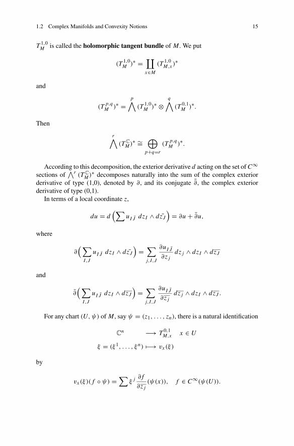
1.2 Complex Manifolds and Convexity Notions 15
T1,0M is called the holomorphic tangent bundle of M . We put
(T1,0M )∗ =
∐
x∈M(T
1,0M,x)
∗
and
(Tp,qM )∗ =
p∧(T
1,0M )∗ ⊗
q∧(T
0,1M )∗.
Then
r∧(T C
M)∗ ∼=
⊕p+q=r
(Tp,qM )∗.
According to this decomposition, the exterior derivative d acting on the set ofC∞sections of
∧r(T C
M)∗ decomposes naturally into the sum of the complex exterior
derivative of type (1,0), denoted by ∂ , and its conjugate ∂ , the complex exteriorderivative of type (0,1).
In terms of a local coordinate z,
du = d(∑
uIJ dzI ∧ dzJ)= ∂u+ ∂u,
where
∂(∑I,J
uI J dzI ∧ dzJ)=∑j,I,J
∂uI J
∂zjdzj ∧ dzI ∧ dzJ
and
∂(∑I,J
uI J dzI ∧ dzJ)=∑j,I,J
∂uI J
∂zjdzj ∧ dzI ∧ dzJ .
For any chart (U,ψ) of M , say ψ = (z1, . . . , zn), there is a natural identification
Cn −→ T
0,1M,x x ∈ U
ξ = (ξ1, . . . , ξn) �−→ vx(ξ)
by
vx(ξ)(f ◦ ψ) =∑
ξj∂f
∂zj(ψ(x)), f ∈ C∞(ψ(U)).
16 1 Basic Notions and Classical Results
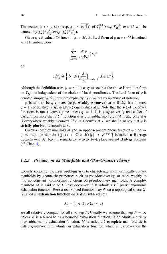
The section x �→ νx(ξ) (resp. x �→ νx(ξ)) of T 0,1M (resp.T
1,0M ) over U will be
denoted by∑
ξj ∂∂zj
(resp.∑
ξj ∂∂zj
).
Given a real-valued C2 function ϕ on M , the Levi form of ϕ at x ∈ M is definedas a Hermitian form
n∑j,k=1
∂2ϕ
∂zj ∂zkξ j ξk
on
T1,0M,x∼={∑
ξj( ∂
∂zj
)z=ψ(x); ξ ∈ C
n}.
Although the definition uses ψ = z, it is easy to see that the above Hermitian formon T
1,0M,x is independent of the choice of local coordinates. The Levi form of ϕ is
denoted simply by Lϕ , or more explicitly by ∂∂ϕ, but by an abuse of notation.ϕ is said to be q-convex (resp. weakly q-convex) at x if Lϕ has at most
q − 1 nonpositive (resp. negative) eigenvalues at x. Note that the set of q-convexfunctions is not a convex cone unless q = 1. It is easy to verify and a fact ofbasic importance that a C2 function ϕ is plurisubharmonic on M if and only if ϕis everywhere weakly 1-convex. If ϕ is 1-convex at x, we shall also say that ϕ isstrictly plurisubharmonic at x.
Given a complex manifold M and an upper semicontinuous function ϕ : M →[−∞,∞), the domain {(ζ, x) ∈ C × M; |ζ | < e−ϕ(x)} is called a Hartogsdomain over M . Recent remarkable activity took place around Hartogs domains(cf. Chap. 4).
1.2.3 Pseudoconvex Manifolds and Oka–Grauert Theory
Loosely speaking, the Levi problem asks to characterize holomorphically convexmanifolds by geometric properties such as pseudoconvexity, or more weakly tofind nonconstant holomorphic functions on pseudoconvex manifolds. A complexmanifold M is said to be Cr -pseudoconvex if M admits a Cr plurisubharmonicexhaustion function. Here a real-valued function, say Ψ on a topological space X,is called an exhaustion function on X if its sublevel sets
Xc = {x ∈ X;Ψ (x) < c}
are all relatively compact for all c < supΨ . Usually we assume that supΨ = ∞unless Ψ is referred to as a bounded exhaustion function. If M admits a strictlyplurisubharmonic exhaustion function, M is called a 1-complete manifold. M iscalled q-convex if it admits an exhaustion function which is q-convex on the
1.2 Complex Manifolds and Convexity Notions 17
complement of a compact subset of M . It is easy to see that every 1-convexmanifold is C∞-pseudoconvex. In fact, if M admits a C2 exhaustion function Ψ
such that LΨ is positive definite on M \ Mc, M also admits a C∞ exhaustionfunction, say Ψ , which is strictly plurisubharmonic outside a compact subset ofM . Such a function Ψ is obtained by approximating Ψ by a C∞ function in theC2 topology. Then, λ(Ψ ) is a C∞ plurisubharmonic exhaustion function on M
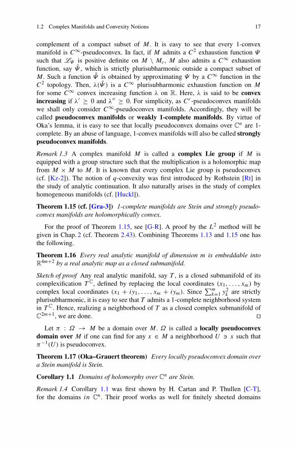
for some C∞ convex increasing function λ on R. Here, λ is said to be convexincreasing if λ′ ≥ 0 and λ′′ ≥ 0. For simplicity, as Cr -pseudoconvex manifoldswe shall only consider C∞-pseudoconvex manifolds. Accordingly, they will becalled pseudoconvex manifolds or weakly 1-complete manifolds. By virtue ofOka’s lemma, it is easy to see that locally pseudoconvex domains over Cn are 1-complete. By an abuse of language, 1-convex manifolds will also be called stronglypseudoconvex manifolds.
Remark 1.3 A complex manifold M is called a complex Lie group if M isequipped with a group structure such that the multiplication is a holomorphic mapfrom M × M to M . It is known that every complex Lie group is pseudoconvex(cf. [Kz-2]). The notion of q-convexity was first introduced by Rothstein [Rt] inthe study of analytic continuation. It also naturally arises in the study of complexhomogeneous manifolds (cf. [Huckl]).
Theorem 1.15 (cf. [Gra-3]) 1-complete manifolds are Stein and strongly pseudo-convex manifolds are holomorphically convex.
For the proof of Theorem 1.15, see [G-R]. A proof by the L2 method will begiven in Chap. 2 (cf. Theorem 2.43). Combining Theorems 1.13 and 1.15 one hasthe following.
Theorem 1.16 Every real analytic manifold of dimension m is embeddable intoR
4m+2 by a real analytic map as a closed submanifold.
Sketch of proof Any real analytic manifold, say T , is a closed submanifold of itscomplexification T C, defined by replacing the local coordinates (x1, . . . , xm) bycomplex local coordinates (x1 + iy1, . . . , xm + iym). Since
∑mk=1 y
2k are strictly
plurisubharmonic, it is easy to see that T admits a 1-complete neighborhood systemin T C. Hence, realizing a neighborhood of T as a closed complex submanifold ofC
2m+1, we are done. ��Let π : Ω → M be a domain over M . Ω is called a locally pseudoconvex
domain over M if one can find for any x ∈ M a neighborhood U � x such thatπ−1(U) is pseudoconvex.
Theorem 1.17 (Oka–Grauert theorem) Every locally pseudoconvex domain overa Stein manifold is Stein.
Corollary 1.1 Domains of holomorphy over Cn are Stein.
Remark 1.4 Corollary 1.1 was first shown by H. Cartan and P. Thullen [C-T],for the domains in C
n. Their proof works as well for finitely sheeted domains

18 1 Basic Notions and Classical Results
over Cn. It is remarkable that the generalization to the infinitely sheeted case wasestablished only after Oka’s work [O-4] which identified holomorphic convexitywith 1-completeness for domains over C
n. As a generalization of Theorem 1.17,it is known that every locally pseudoconvex domain over CPn is pseudoconvex (cf.Theorem 2.73). As a result, a locally pseudoconvex domain over CPn is Stein unlessit is biholomorphic to CP
n itself. The L2 method of Hörmander [Hö-1, Hö-2] is aquantitative approach to further generalizations of Theorems 1.15 and 1.17.
If D is a domain with smooth boundary in a complex manifold M , localpseudoconvexity is a property of the Levi form of a function defining the boundary∂D. To describe the boundary behavior of holomorphic functions, the Levi form ofa defining function of ∂D is important. It is basic that local pseudoconvexity of Dis characterized by an extrinsic but essentially intrinsic geometric property of ∂D.
Let D be a domain in M . For any r ≥ 1, D is said to be Cr -smooth if there existsa real-valued Cr function, say ρ on a neighborhood U of ∂D such that
D ∩ U = {z ∈ U ; ρ(z) < 0}
and dρ vanishes nowhere on ∂D. We shall call ρ a defining function of ∂D, orsometimes that of D if ρ is defined on D ∪ U . We put
T1,0∂D = T
1,0M ∩ (T∂D ⊗ C).
If D is C2-smooth and Lρ |T 1,0∂D
is everywhere semipositive on ∂D for some
defining function ρ of D, ∂D is said to be pseudoconvex. ∂D is called stronglypseudoconvex at x ∈ ∂D if Lρ |T 1,0
∂Dis positive definite at x.
Definition 1.8 A strongly pseudoconvex domain in M is a relatively compactdomain in M whose boundary is everywhere strongly pseudoconvex.
Strongly pseudoconvex domains admit strictly plurisubharmonic defining func-tions. In fact, for any defining function ρ of D, eAρ − 1 becomes strictlyplurisubharmonic on a neighborhood of ∂D for sufficiently large A. Stronglypseudoconvex domains are 1-convex because − log (−ρ) is an exhaustion functionon D which is plurisubharmonic outside a compact subset of D.
Remark 1.5 A smoothly bounded pseudoconvex domain is called weakly pseu-doconvex if it is not strongly pseudoconvex. There exist Cω-smooth weaklypseudoconvex domains which do not admit plurisubharmonic defining functions(cf. [B]). For a further extensive account of the Levi problem, see [Siu’78].
1.3 Oka–Cartan Theory 19
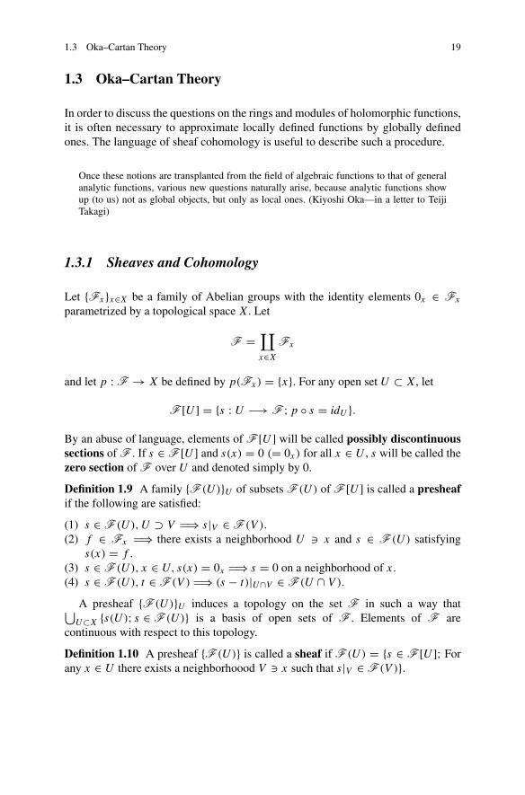
1.3 Oka–Cartan Theory
In order to discuss the questions on the rings and modules of holomorphic functions,it is often necessary to approximate locally defined functions by globally definedones. The language of sheaf cohomology is useful to describe such a procedure.
Once these notions are transplanted from the field of algebraic functions to that of generalanalytic functions, various new questions naturally arise, because analytic functions showup (to us) not as global objects, but only as local ones. (Kiyoshi Oka—in a letter to TeijiTakagi)
1.3.1 Sheaves and Cohomology
Let {Fx}x∈X be a family of Abelian groups with the identity elements 0x ∈ Fx
parametrized by a topological space X. Let
F =∐
x∈XFx
and let p : F → X be defined by p(Fx) = {x}. For any open set U ⊂ X, let
F [U ] = {s : U −→ F ;p ◦ s = idU }.
By an abuse of language, elements of F [U ] will be called possibly discontinuoussections of F . If s ∈ F [U ] and s(x) = 0 (= 0x) for all x ∈ U , s will be called thezero section of F over U and denoted simply by 0.
Definition 1.9 A family {F (U)}U of subsets F (U) of F [U ] is called a presheafif the following are satisfied:
(1) s ∈ F (U), U ⊃ V �⇒ s|V ∈ F (V ).
(2) f ∈ Fx �⇒ there exists a neighborhood U � x and s ∈ F (U) satisfyings(x) = f .
(3) s ∈ F (U), x ∈ U, s(x) = 0x �⇒ s = 0 on a neighborhood of x.(4) s ∈ F (U), t ∈ F (V ) �⇒ (s − t)|U∩V ∈ F (U ∩ V ).
A presheaf {F (U)}U induces a topology on the set F in such a way that⋃U⊂X {s(U); s ∈ F (U)} is a basis of open sets of F . Elements of F are
continuous with respect to this topology.
Definition 1.10 A presheaf {F (U)} is called a sheaf if F (U) = {s ∈ F [U ]; Forany x ∈ U there exists a neighborhoood V � x such that s|V ∈ F (V )}.

20 1 Basic Notions and Classical Results
Clearly, for any presheaf {F (U)} (an abbreviation for {F (U)}U ), one can find asheaf {F (U)} such that F (U) ⊂ F (U) ⊂ F [U ] uniquely. {F (U)} will be calledthe sheafification of {F (U)}.
For simplicity, the topological space F will also stand for the sheaf {F (U)}. Tobe explicit, F is called a sheaf over X. The map p : F → X will be referred to asa sheaf projection.
Fx is called a stalk of F at x, and the elements of Fx the germs at x. Elementsof F (U) will be called the sections of F over U . By (3) above, the germs at x ofsections in F (U) are naturally identified with elements of Fx if U � x, i.e.
Fx = ind.limU�xF (U)
with respect to the inductive system induced from the natural restriction mapsF [U ] → F [V ] for U ⊃ V � x. For any s ∈ F [U ] the germ of s at x willbe denoted by sx . In short, s(x) = sx if s ∈ F (U). Let G be another sheaf overX. G is called a subsheaf of F if G (U) ⊂ F (U) for any open set U ⊂ X. Theconstant sheaf CX → X is defined as the sheaf whose stalks are C. CX will besimply denoted by C.
Note that the family {F [U ]} itself is not necessarily a sheaf because thecondition (3) may not be satisfied. However, if we put
Fx = ind.limU�xF [U ],F =
∐
x�XFx
and
F (U) = {s : U −→ F ; s(x) = sx for some s ∈ F [U ]},
then {F (U)}U is a sheaf over X. F has a property that any section over anyopen set extends to X as a section. Sheaves having this property are called flabbysheaves. Since F is a subsheaf of F , we shall call the sheaf F the canonicalflabby extension of F .
For any two sheaves Fj (j = 1, 2) over X, the direct sum F1 ⊕F2 is a sheafdefined by {F1(U) ⊕F2(U)}U . For any continuous map β : X → Y , the directimage sheaf of F by β, denoted by β∗F , is defined over Y by
(β∗F )x = ind.limU�xF1(β−1(U))
and (β∗F )(U) = F (β−1(U)).If A ⊂ X, the sheaf
∐x∈A Fx is denoted by F |A. Here F |A(U) :=
ind.limV⊃UF (V ). F |A is called the restriction of F to A. A is called the supportof F if “Fx = {0x} ⇔ x /∈ A ”. The support of F is denoted by supp F .
Sheaves of rings and sheaves of modules are defined similarly.

1.3 Oka–Cartan Theory 21
Definition 1.11 A ringed space is a topological space equipped with a sheaf ofrings.
For any complex manifold M , the family {O(U);U is open in M} is naturallyregarded as a sheaf by identifying an element of O(U) as the collection of its germs.This sheaf is called the structure sheaf of M and denoted by OM , or simply by O .(M,O) is the most important example of ringed space for our purpose. We note thatthe domains of holomorphy are nothing but the connected components of OCn . Formeromorphic functions, domains of meromorphy can be characterized similarly.Namely, in the sheaf theoretic terms, meromorphic functions are identified as thesections of a sheaf in the following way: Let Mx be the quotient field of Ox , let
M =∐
x∈MMx,
and
M (U) = {h ∈M [U ]; for every x ∈ U there exist a neighborhood V � x and
f, g ∈ O(V ) such that h(y) = fy
gyfor all y ∈ V }
for any open set U ⊂ M . Sections of the sheaf {M (U)}U are called meromorphicfunctions. Connected components of the sheaf M as the topological space arecalled the domains of meromorphy.
A sheaf p1 : F1 → X1 is said to be isomorphic to a sheaf p2 : F2 → X2 ifthere exists a homeomorphism ψ : X1 → X2 and a bijection β : F1 → F2 suchthat
β|F1,x ∈ Hom(F1,x,F2,ψ(x))
for all x ∈ X1.Complex manifolds are naturally identified with ringed spaces which are locally
isomorphic to (D,OD) for some domain D in Cn.
Definition 1.12 An ideal sheaf of a ringed space (X,R) is a sheaf of R-modules(X,I ) such that Ix is an ideal of Rx for each x ∈ X.
Let R → X be a sheaf of commutative rings with units and let Ej → X (j =1, 2) be sheaves of R-modules (i.e. Ej,x are Rx-modules, etc.). A collection ofRx-homomorphisms
αx : E1,x −→ E2,x, x ∈ X,
denoted by α : E1 → E2 is called a homomorphism between R-modules if
s ∈ E1(U) �⇒ α ◦ s ∈ E2(U)

22 1 Basic Notions and Classical Results
holds for any open setU ⊂ X. α◦s will also be denoted by α(s) (for a typographicalreason). For the sheaves of Abelian groups and those of rings, homomorphisms aredefined similarly. Sheaves of O-modules are called analytic sheaves.
The stalkwise direct sum R⊕m is called a free R-module of rank m. A sheaf ofR-modules is called locally free if it is locally isomorphic to a free sheaf. Locallyfree sheaves of rank one are said to be invertible. A sheaf E of R-modules is saidto be torsion free if Ex are torsion free Rx-modules. Locally free R-modules aretorsion free.
A holomorphic map ψ between two complex manifolds (Mj ,Oj ) (j = 1, 2)induces a homomorphism
ψ∗ : O2|ψ(M1) −→ ψ∗O1|ψ(M1)
by ψ∗(fψ(x)) = (f ◦ ψ)ψ(x). Conversely, a continuous map ψ : M1 → M2 isholomorphic if there exists a homomorphism β : O2|ψ(M1) → ψ∗O1|ψ(M1) whichinduces at every point x ∈ M1 a homomorphism from O2,ψ(x) to O1,x which mapsthe invertible elements of O2,ψ(x) to those of O1,x .
For any homomorphism α : E1 → E2, the collection of preimages of 0, which iscalled the kernel of α, is naturally equipped with a sheaf structure whose sectionsover U are precisely the elements of {s ∈ E1(U);α ◦ s = 0}, the kernel of thehomomorphism
αU : E1(U) � s −→ α ◦ s ∈ E2(U).
The kernel of α will be denoted by Kerα. Definition of the cokernel of α is moredelicate: Let
cokerα =∐
x∈Xcokerαx,
let π : E2 →∐x∈X cokerαx be the canonical projection, and let
cokerα(U) = {s ∈ cokerα[U ]; s = π ◦ s for some s ∈ E2(U)}.
Then {cokerα(U)} is clearly a presheaf. The sheafification of {cokerα(U)} will becalled the cokernel sheaf of α and denoted by Cokerα. When α is an inclusion,Cokerα will be denoted by E1/E2. The image sheaf Imα of α is defined similarly.Given an ideal sheaf I of R, the cokernel R/I of the inclusion morphism ι :I → R carries naturally the induced structure of a sheaf of commutative rings.
A sequence
· · · −→ E k −→ E k+1 −→ E k+2 −→ · · · (1.4)
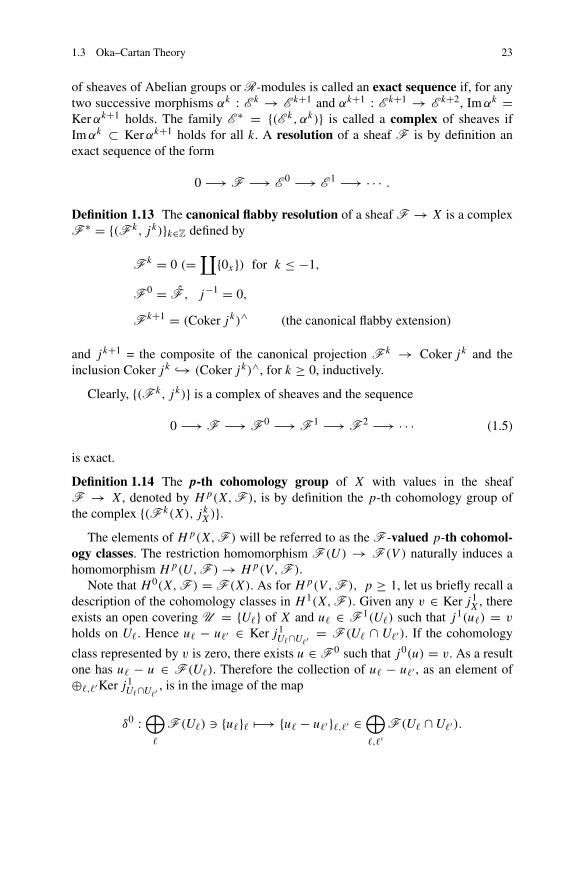
1.3 Oka–Cartan Theory 23
of sheaves of Abelian groups or R-modules is called an exact sequence if, for anytwo successive morphisms αk : E k → E k+1 and αk+1 : E k+1 → E k+2, Imαk =Kerαk+1 holds. The family E ∗ = {(E k, αk)} is called a complex of sheaves ifImαk ⊂ Kerαk+1 holds for all k. A resolution of a sheaf F is by definition anexact sequence of the form
0 −→ F −→ E 0 −→ E 1 −→ · · · .
Definition 1.13 The canonical flabby resolution of a sheaf F → X is a complexF ∗ = {(F k, jk)}k∈Z defined by
F k = 0 (=∐{0x}) for k ≤ −1,
F 0 = F , j−1 = 0,
F k+1 = (Coker jk)∧ (the canonical flabby extension)
and jk+1 = the composite of the canonical projection F k → Coker jk and theinclusion Coker jk ↪→ (Coker jk)∧, for k ≥ 0, inductively.
Clearly, {(F k, jk)} is a complex of sheaves and the sequence
0 −→ F −→ F 0 −→ F 1 −→ F 2 −→ · · · (1.5)
is exact.
Definition 1.14 The p-th cohomology group of X with values in the sheafF → X, denoted by Hp(X,F ), is by definition the p-th cohomology group ofthe complex {(F k(X), jkX)}.
The elements of Hp(X,F ) will be referred to as the F -valued p-th cohomol-ogy classes. The restriction homomorphism F (U) → F (V ) naturally induces ahomomorphism Hp(U,F )→ Hp(V,F ).
Note that H 0(X,F ) = F (X). As for Hp(V,F ), p ≥ 1, let us briefly recall adescription of the cohomology classes in H 1(X,F ). Given any v ∈ Ker j1
X, thereexists an open covering U = {U�} of X and u� ∈ F 1(U�) such that j1(u�) = v
holds on U�. Hence u� − u�′ ∈ Ker j1U�∩U�′ = F (U� ∩ U�′). If the cohomology
class represented by v is zero, there exists u ∈ F 0 such that j0(u) = v. As a resultone has u� − u ∈ F (U�). Therefore the collection of u� − u�′ , as an element of⊕�,�′Ker j1
U�∩U�′ , is in the image of the map
δ0 :⊕�
F (U�) � {u�}� �−→ {u� − u�′ }�,�′ ∈⊕�,�′
F (U� ∩ U�′).

24 1 Basic Notions and Classical Results
Consequently, letting
Cp(U ,F ) =⊕
�0,...,�p
{u�0...�p ∈ F (U�0 ∩ · · · ∩ U�p); u�0...�p
is alternating in �0, . . . , �p}
and defining
δp
U : Cp(U ,F ) −→ Cp+1(U ,F )
and Hp(U ,F ) respectively by
δp
U ({u�0...�p }�0,...,�p ) ={ ∑
0≤j≤p(−1)ju�′0...�′j−1�
′j+1...�
′p+1
}�′0,...,�′p+1
and Ker δpU /Im δp−1U , one has a homomorphism
γ 1 : H 1(X,F ) −→ ind.limU H 1(U ,F )
defined by the correspondence [v] → [{u� − u′�}�,�′ ], and similarly γ p :Hp(X,F ) → ind.limU Hp(U ,F ) for all p. Here the inductive system{Hp(U ,F )} is with respect to the restriction homomorphisms Hp(U ,F ) →Hp(V ,F ) for the refinements V of U . See [G-R] (for instance) for the detailof the construction of γ p for p ≥ 1 and for the proof of the following extremelyimportant fact.
Theorem 1.18 γ p are isomorphisms if X is a paracompact Hausdorff space.
For any paracompact Hausdorff space X, a sheaf G → X of Abelian groupsis said to be fine if, given any open covering U of X, there exists a locally finiterefinement V = {Vj } of U and homomorphisms hj : G → G such that
supp hj := {x ; hj | Gx �= 0} ⊂ Vj
and∑
j hj = 1.
Corollary of Theorem 1.18. If G → X is a fine sheaf,
Hp(X,G ) = 0
for any p ≥ 1.A resolution 0 → F → E 0 → E 1 → · · · is said to be fine if E k are fine
sheaves.Another basic fact is the existence of a canonically defined exact sequences of
the cohomology groups: Let

1.3 Oka–Cartan Theory 25
0 −→ E −→ F −→ G −→ 0 (1.6)
be an exact sequence of sheaves over X. Then it is easy to see that the inducedsequence
0 −→ E (X) −→ F (X) −→ G (X)
is exact. By the exactness of (1.6), this sequence can be prolonged canonically as
E (X)→ F (X)→ G (X)→ H 1(X,E )→ H 1(X,F )
→ H 1(X,G )→ H 2(X,E )→ · · · ,
which is called the long exact sequence associated to (1.6) (cf. [G-R]).
1.3.2 Coherent Sheaves, Complex Spaces, and Theorems Aand B
In the study of ideals of holomorphic functions, Oka and Cartan were led tointroduce a notion characterizing a class of ideal sheaves of O , the coherence (cf.[O-2] and [C]).
Definition 1.15 An R-module E over a topological space X is called coherentif:
(1) E is locally finitely generated, i.e. for any x0 ∈ X there exist a neighborhoodU � x0 and finitely many sections of M overU whose values at x ∈ U generateEx over Rx for any x ∈ U .
(2) For any m ∈ N and for any morphism α from the direct sum R⊕m to E , Kerαis locally finitely generated.
A penetrating insight (definitely shared by Oka and Cartan) was that a principalbasic question of several complex variables is to establish a criterion for the analyticsheaves to be globally generated.
For any complex manifold (M,O), Oka established the following basic resultby exploiting the Weierstrass division theorem to run an induction argument on thedimension.
Theorem 1.19 (Oka’s coherence theorem) O is coherent.
For the proof, the reader is referred to [G-R, Hö-2], or [Nog]. By this theorem,for any coherent O-module F and for any x ∈ M , one can find a neighborhoodU � x and an exact sequence over U of the form
· · · −→ O⊕mk |U −→ · · · −→ O⊕m2 |U −→ O⊕m1 |U −→ F |U −→ 0,

26 1 Basic Notions and Classical Results
which is called a free resolution of F overU . Since C{z1, . . . , zn} is a regular localring of dimension n, the kernel of O⊕mn |U → O⊕mn−1 |U is locally free by Hilbert’ssyzygy theorem (cf. [G-R]).
For any A ⊂ M , IA will stand for the ideal sheaf of O consisting of the germsof holomorphic functions vanishing along A, i.e.
IA(U) = {f ∈ O(U); f |U∩A = 0}.
IA is called the ideal sheaf of A, for short.
Definition 1.16 A closed set A ⊂ M is called an analytic set if for every pointx ∈ A there exist a neighborhood U , m ∈ N, and f1, . . . , fm ∈ O(U) such thatU ∩ A = {w ∈ U ; f1(w) = · · · = fm(w) = 0}.
From the definition, it is clear that supp(O/I ) is analytic if I is a coherentideal sheaf. The vector-valued holomorphic function (f1, . . . , fm) is called a localdefining function of A around x. By the dimension of an analytic set A at x ∈ A,we shall mean the minimal number of holomorphic functions f1, . . . , fk defined ona neighborhood of U such that x is isolated in A ∩ (⋂k
j=1 f−1j (0)).
Theorem 1.20 (Rückert’s Nullstellensatz) Let (f1, . . . , fm) be a local definingfunction of an analytic set A around x and let f ∈ IA,x . Then there exists p ∈ N
such that
f p ∈m∑j=1
fj · OM,x.
For the proof, the reader is referred to [G-R, Chapter 3, A].
Theorem 1.21 (Cartan’s coherence theorem) IA is coherent if A is analytic.
Sketch of proof Let x ∈ A, let (f1, . . . , fm) be a local defining function ofA aroundx, and let IA be the ideal sheaf generated by fj (1 ≤ j ≤ m) over a neighborhoodU � x. Then one has an exact sequence of O-modules
0 −→ IA −→ IA|U −→ IA|U/IA −→ 0.
Since IA is coherent by Theorem 1.19, the coherence of IA follows by adescending induction on the codimension of A. ��Remark 1.6 The ideal sheaf J of the form
Jx ={fx ∈ Ox;
∫U
|f |2e−ϕ dλ <∞ for some neighborhood U of x}
turns out to be coherent if ϕ is plurisubharmonic (see Chap. 3).

1.3 Oka–Cartan Theory 27
Roughly speaking, complex spaces are complex manifolds with singularities. Infunction theory, such things arise as ringed spaces which are locally isomorphicto those whose underlying spaces are the sets of common zeros of holomorphicfunctions.
Definition 1.17 A ringed space (X,O) is called a complex space if everypoint x ∈ X has a neighborhood U such that (U,O|U) is isomorphic to(supp(OD/I ),OD/I ) for some domain D in C
N (N = N(x)) and for somecoherent ideal sheaf I of OD .
Example 1.7 Let D be a domain in Cn, let F ∈ O(D), let X = F−1(0) and let
O = OD/F · OD . Then (X,O) is a complex space, since F · OD is coherent byTheorem 1.19.
X will be referred to as the underlying space of the complex space (X,O).(X,O) is said to be compact if so is the underlying space X. A point x ∈ X is calleda regular point of (X,O) if one can find U and D such that O|U ∼= OD . The set ofregular points of X is denoted by Xreg. X \ Xreg is denoted by SingX. O is calledthe structure sheaf of X. The structure sheaf is denoted also by OX. Coherent O-sheaves will be called coherent analytic sheaves. A closed set A ⊂ X is called ananalytic set if it is the support of some coherent analytic sheaf over X. An analyticset ofX is naturally equipped with the structure of a reduced complex space inducedfrom OX (see Definition 1.18 below). Analytic sets of CPn are called projectivealgebraic sets. The implicit function theorem naturally implies that SingX is ananalytic set of X. X is called nonsingular if SingX = ∅. (X,O) is said to beirreducible if every proper analytic set is nowhere dense. An irreducible complexspace (Y,OY ) is called an irreducible component of (X,OX) if Y ⊂ X and theinclusion map ι : Y → X is accompanied with a surjective sheaf homomorphismOX|Y → ι∗OY |Y whose kernel has a nowhere dense support in Y . Irreduciblecomplex spaces are called varieties.
By a routine argument one can infer the following from Theorem 1.19.
Theorem 1.22 The structure sheaf of a complex space is coherent.
For any complex space (X,O), the elements of O(X)will be called holomorphicfunctions on X. Holomorphic functions on X naturally induce genuine C-valuedfunctions onX. If a holomorphic function f onX is zero as a function, then, for eachx ∈ X fx is nilpotent, i.e. some power of fx is zero, by Rückert’s Nullstellensatz.By an abuse of notation, the values of f in C will be denoted by f (x).
Given two complex spaces (X,OX) and (Y,OY ), a holomorphic map from(X,OX) to (Y,OY ) is by definition a pair of continuous map ψ : X → Y and ahomomorphism
β : OY |ψ(X) −→ ψ∗OX|ψ(X)between the sheaves of rings which maps invertible elements to invertible elements.

28 1 Basic Notions and Classical Results
For any holomorphic map (ψ, β) from (X,OX) to (Y,OY ), a homomorphismfrom Hp(Y,OY ) to Hp(X,OX) is induced canonically. For simplicity, (ψ, β) willbe referred to as ψ and the induced homomorphism Hp(Y,OY )→ Hp(X,OX) byψ∗.
Definition 1.18 A complex space (X,O) is said to be reduced if no stalk of Ocontains a nilpotent element.
For any reduced complex space (X,O) and f, g ∈ O(X), f = g if and only iff (x) = g(x)(∈ C) for all x ∈ X. For any complex space (X,O), the collection ofthe nilpotent elements in the stalks of O is an ideal sheaf, say J . Then (X,O/J )
is a reduced complex space. We shall call it the reduction of (X,O).If (X,O) is reduced, Xreg is an everywhere dense subset of X. We then define
the dimension of X by dimX := dimXreg and put
dimx X = sup {dim Ureg;U is a neighborhood of x} for any x ∈ X.
dim X and dimx X will stand for those for the reduction of (X,O). It is easy toverify that this definition of the dimension agrees with that for analytic sets when(X,O) = (A,O/IA). The codimension of A ⊂ X is defined as dim X − dim A.It will be denoted by codimX A. X is called a complex curve if dimX = 1.
Definition 1.19 A complex space (X,O) is called a Stein space (resp. a holomor-phically convex space) if any discrete closed subset of X is mapped injectively(resp. properly) into a discrete closed subset of C by a holomorphic function on X.
Theorem 1.23 (Cartan’s theorem A) Let (X,O) be a Stein space. Then, for anycoherent analytic sheaf F over X and for any point x ∈ X, the image of the naturalrestriction map
F (X) −→ Fx
generates Fx over Ox .
Combining Theorem 1.23 with Cartan’s coherence theorem, we obtain forinstance the following.
Proposition 1.1 Let (X,O) be a Stein space, let A ⊂ M be an analytic set, and letx ∈ A be any point. Then there exist a neighborhoodU � x and f1, . . . , fm ∈ O(X)
such that U ∩ A = {y ∈ U ; f1(y) = · · · = fm(y) = 0}.Theorem 1.23 was first established by Oka when X is a domain of holomorphy
in Cn and F is a coherent ideal sheaf (idéal de domaine indéterminé) over X. For
the proof, Oka and Cartan solved a problem which P. Cousin had solved in 1895in a very special case to construct meromorphic functions with given poles on theproducts of plane domains. This argument was extended eventually to show thatTheorem 1.23 is a consequence of the assertion that H 1(X,F ) = 0 holds for any

1.3 Oka–Cartan Theory 29
coherent analytic sheaf over a Stein space (X,O). An ultimately strengthend formof such a cohomology vanishing theorem on Stein spaces is the following.
Theorem 1.24 (Cartan’s theorem B) Hp(X,F ) = 0 for any p ≥ 1 if F is acoherent analytic sheaf over a Stein space (X,O).
There are a lot of implications of the vanishing of cohomology groups. It may beworthwhile to recall that there is a characterization of Stein spaces among them.
Theorem 1.25 (X,O) is a Stein space if and only if H 1(X,I ) = 0 for anycoherent ideal sheaf of O .
Proof For any discrete closed set Γ ⊂ X, the ideal sheaf IΓ of Γ is coherent byTheorem 1.21. Hence H 1(X,IΓ ) = 0, so that from the exact sequence
0 −→ IΓ −→ OX −→ OX/IΓ −→ 0
one has the surjectivity of the natural restriction homomorphism O(X)→ CΓ . ��
Remark 1.7 The surjectivity of O(X) → CΓ is equivalent to the injectivity of
H 1(X,I )→ H 1(X,O) by the long exact sequence. This point has a significancein the development of the application of the L2 technique. If (X,O) is a domainover C
n, it is easy to see that X is Stein if and only if Hq(X,O) = 0 for any1 ≤ q ≤ n − 1 (cf. [Oh-21, 2.3]). Actually, Hn(X,O) = 0 holds whenever X is acomplex space of dimension n which does not contain any compact n-dimensionalanalytic subset (cf. [Siu-1]).
Once it is recognized that Theorem 1.23 is a consequence of a vanishing theorem asabove, it is not difficult to show the following for instance.
Theorem 1.26 (cf. [Gra-2]) Every analytic subset of a Stein space of dimension nis the set of common zeros of at most n+ 1 holomorphic functions.
Remark 1.8 Forster and Ramspott [F-R] proved that actually n functions suffice. Itwas known by Kronecker [K] that every algebraic set in C
n is the set of commonzeros of n+1 polynomials. Eisenbud and Evans proved in [Eb-E] that n polynomialssuffice. This theory is closely related to the Oka principle asserting the categoricalequivalence between topology and analysis on Stein manifolds. (See [F’17] for thedetail.)
The L2 method provides another effective way to analyze the sheaf cohomologygroups. As a result, Theorem 1.24 can be extended to pseudoconvex spaces andcertain ideal sheaves arising naturally in basic questions of complex geometry. (SeeChap. 3.)

30 1 Basic Notions and Classical Results
1.3.3 Coherence of Direct Images and a Theorem of Andreottiand Grauert
A complex space (X,O) is said to be normal if, for any open set U ⊂ X andfor any nowhere-dense analytic set A ⊂ U , bounded holomorphic functions onU \A extend holomorphically to U . It is easy to see that normal complex curves arenonsingular. In [O-3], Oka proved that every reduced complex space has a “normalmodel”, i.e. for any reduced complex space (X,O) there exist a reduced complexspace (X,O
X) and a proper surjective holomorphic map p : X → X such that
p|p−1(Xreg)is a biholomorphic map onto Xreg and the inclusion map ι : Xreg ↪→ X
induces an isomorphism ι∗O ∼= OX
. It can be stated as another coherence theoremas follows.
Theorem 1.27 (Oka’s normalization theorem) Let (X,O) be a reduced complexspace and let ι : Xreg → X be the inclusion map. Then the direct image sheafι∗OXreg is a coherent sheaf of rings if dimx SingX+ 2 ≤ lim infy→x dimy X for allx ∈ SingX.
Substantially, this is a primitive form of Hironaka’s desingularization theorem.Recall that Hironaka’s desingularization theorem asserts that every reduced complexspace has a nonsingular model, i.e. for any reduced complex space (X,OX) one canfind a complex manifold (M,OM) and a proper holomorphic map π : M → X suchthat π |M\π−1(SingX) is a biholomorphic map onto Xreg.
Let ψ : X → Y be a holomorphic map. For any analytic sheaf F → X, thep-th direct image sheaf of F , denoted by Rpψ∗F , is defined as the sheafificationof the presheaf
U −→ {s : U →∐
y�U(ind.limV�yHp(ψ−1(V ),F ));
there exists u ∈ Hp(ψ−1(U),F ) such that s(y) = uy for all y}.
Note that R0ψ∗F = ψ∗F . The following is a very profound result.
Theorem 1.28 (cf. [Gra-4, Gra-R-2]) Let ψ : X → Y be a proper holomorphicmap between complex spaces and let F → X be a coherent analytic sheaf. ThenRpψ∗F (p ≥ 0) are coherent analytic sheaves over Y .
Corollary 1.2 (Remmert’s proper mapping theorem) For any proper holomor-phic map ψ : X→ Y , ψ(X) is an analytic set of Y .
Theorem 1.28 is a generalization of the following.
Theorem 1.29 (Cartan–Serre finiteness theorem) For any compact complexspace (X,O) and for any coherent analytic sheaf F over X, dimHp(X,F ) <∞for all p.
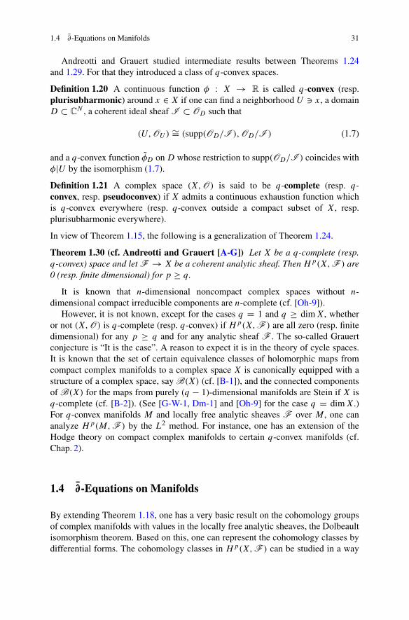
1.4 ∂-Equations on Manifolds 31
Andreotti and Grauert studied intermediate results between Theorems 1.24and 1.29. For that they introduced a class of q-convex spaces.
Definition 1.20 A continuous function φ : X → R is called q-convex (resp.plurisubharmonic) around x ∈ X if one can find a neighborhood U � x, a domainD ⊂ C
N , a coherent ideal sheaf I ⊂ OD such that
(U,OU) ∼= (supp(OD/I ),OD/I ) (1.7)
and a q-convex function φD on D whose restriction to supp(OD/I ) coincides withφ|U by the isomorphism (1.7).
Definition 1.21 A complex space (X,O) is said to be q-complete (resp. q-convex, resp. pseudoconvex) if X admits a continuous exhaustion function whichis q-convex everywhere (resp. q-convex outside a compact subset of X, resp.plurisubharmonic everywhere).
In view of Theorem 1.15, the following is a generalization of Theorem 1.24.
Theorem 1.30 (cf. Andreotti and Grauert [A-G]) Let X be a q-complete (resp.q-convex) space and let F → X be a coherent analytic sheaf. Then Hp(X,F ) are0 (resp. finite dimensional) for p ≥ q.
It is known that n-dimensional noncompact complex spaces without n-dimensional compact irreducible components are n-complete (cf. [Oh-9]).
However, it is not known, except for the cases q = 1 and q ≥ dimX, whetheror not (X,O) is q-complete (resp. q-convex) if Hp(X,F ) are all zero (resp. finitedimensional) for any p ≥ q and for any analytic sheaf F . The so-called Grauertconjecture is “It is the case”. A reason to expect it is in the theory of cycle spaces.It is known that the set of certain equivalence classes of holomorphic maps fromcompact complex manifolds to a complex space X is canonically equipped with astructure of a complex space, say B(X) (cf. [B-1]), and the connected componentsof B(X) for the maps from purely (q − 1)-dimensional manifolds are Stein if X isq-complete (cf. [B-2]). (See [G-W-1, Dm-1] and [Oh-9] for the case q = dimX.)For q-convex manifolds M and locally free analytic sheaves F over M , one cananalyze Hp(M,F ) by the L2 method. For instance, one has an extension of theHodge theory on compact complex manifolds to certain q-convex manifolds (cf.Chap. 2).
1.4 ∂-Equations on Manifolds
By extending Theorem 1.18, one has a very basic result on the cohomology groupsof complex manifolds with values in the locally free analytic sheaves, the Dolbeaultisomorphism theorem. Based on this, one can represent the cohomology classes bydifferential forms. The cohomology classes in Hp(X,F ) can be studied in a way

32 1 Basic Notions and Classical Results
closely related to the geometry of X and F by exploiting such an expression. Thisis the method of L2 estimates to be discussed in subsequent chapters. Basic notionsneeded for that are holomorphic vector bundles, Dolbeault cohomology groups,Chern connections, curvature forms, etc., which belong to differential geometryand recalled below together with classical results as Dolbeault’s isomorphismtheorem and Serre’s duality theorem, which are natural counterparts of the de Rhamisomorphism and the Poincaré duality in the classical global differential geometry.
1.4.1 Holomorphic Vector Bundles and ∂-Cohomology
A holomorphic vector bundle over a complex manifold is by definition a C∞complex vector bundle whose transition functions are holomorphic. In other words,a complex manifold E is called a holomorphic vector bundle over a complexmanifold M if E is of the form
∐x∈M Ex , as a set for some vector spaces Ex
parametrized by M , satisfying the following requirements:
(1) The map
π : E ⊃ Ex �−→ {x} ⊂ M
is holomorphic and dπ : T 1,0E → T
1,0M is everywhere of maximal rank.
(2) For any open setU ⊂ M , f, g ∈ O(U) and holomorphic sections s, t : U → E,f s + gt is also holomorphic.
The rank of E (= rankE := dim Ker dπ ) is a locally constant function on M ,which will be assumed to be constant unless stated otherwise. From the definition,it is clear that the direct sums, the duals and the tensor products of holomorphicvector bundles are naturally defined by fiberwise construction. They will be denotedby E1 ⊕ E2, E∗ and E1 ⊗ E2, respectively. Hom(E1, E2) will stand for E∗1 ⊗ E2.∧r
E will be denoted by detE if r = rankE. Holomorphic vector bundles overcomplex spaces are defined similarly. For any subset A ⊂ M , E|A will stand forthe vector bundle π−1(A)→ A. A local (holomorphic) frame of E over an openset U is an r-tuple of holomorphic sections, say s1, . . . , sr of E|U → U such thats1(x), . . . , sr (x) are linearly independent for all x ∈ U .
For two holomorphic vector bundles Ej (j = 1, 2) over M , a holomorphic mapα : E1 → E2 is called a bundle homomorphism, or simply a homomorphism, ifα|E1,x ∈ Hom(E1,x, E2,x) for all x ∈ M and dimα(E1,x) is a locally constant func-tion on M . The isomorphism E1 ∼= E2 will mean that there exists a biholomorphicbundle homomorphism from E1 to E2. Given any bundle homomorphism, its kerneland cokernel are naturally defined as holomorphic vector bundles. Subbundles andquotient bundles are defined similarly. A sequence of bundle homomorphisms issaid to be exact if it is exact fiberwise. Given a holomorphic map f : M → N anda holomorphic vector bundle π : E → N , f ∗E will stand for the fiber product off and π , naturally equipped with the structure of a holomorphic vector bundle over
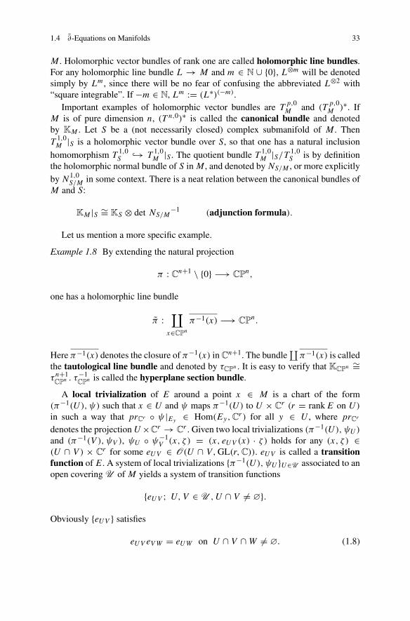
1.4 ∂-Equations on Manifolds 33
M . Holomorphic vector bundles of rank one are called holomorphic line bundles.For any holomorphic line bundle L → M and m ∈ N ∪ {0}, L⊗m will be denotedsimply by Lm, since there will be no fear of confusing the abbreviated L⊗2 with“square integrable”. If −m ∈ N, Lm := (L∗)(−m).
Important examples of holomorphic vector bundles are Tp,0M and (T
p,0M )∗. If
M is of pure dimension n, (T n,0)∗ is called the canonical bundle and denotedby KM . Let S be a (not necessarily closed) complex submanifold of M . ThenT
1,0M |S is a holomorphic vector bundle over S, so that one has a natural inclusion
homomorphism T1,0S ↪→ T
1,0M |S . The quotient bundle T 1,0
M |S/T 1,0S is by definition
the holomorphic normal bundle of S in M , and denoted by NS/M , or more explicitlyby N1,0
S/M in some context. There is a neat relation between the canonical bundles ofM and S:
KM |S ∼= KS ⊗ det NS/M−1 (adjunction formula).
Let us mention a more specific example.
Example 1.8 By extending the natural projection
π : Cn+1 \ {0} −→ CPn,
one has a holomorphic line bundle
π :∐
x∈CPnπ−1(x) −→ CP
n.
Here π−1(x) denotes the closure of π−1(x) in Cn+1. The bundle
∐π−1(x) is called
the tautological line bundle and denoted by τCPn . It is easy to verify that KCPn ∼=
τn+1CP
n . τ−1CP
n is called the hyperplane section bundle.
A local trivialization of E around a point x ∈ M is a chart of the form(π−1(U), ψ) such that x ∈ U and ψ maps π−1(U) to U × C
r (r = rankE on U)
in such a way that prCr ◦ ψ |Ey ∈ Hom(Ey,Cr ) for all y ∈ U , where prCr
denotes the projection U×Cr → C
r . Given two local trivializations (π−1(U), ψU)
and (π−1(V ), ψV ), ψU ◦ ψ−1V (x, ζ ) = (x, eUV (x) · ζ ) holds for any (x, ζ ) ∈
(U ∩ V ) × Cr for some eUV ∈ O(U ∩ V,GL(r,C)). eUV is called a transition
function of E. A system of local trivializations {π−1(U), ψU }U∈U associated to anopen covering U of M yields a system of transition functions
{eUV ; U,V ∈ U , U ∩ V �= ∅}.
Obviously {eUV } satisfies
eUV eVW = eUW on U ∩ V ∩W �= ∅. (1.8)

34 1 Basic Notions and Classical Results
Conversely, given any open covering U of M and a system of GL(r,C)-valuedholomorphic functions eUV (U,V ∈ U ) satisfying the transition relations (1.8), aholomorphic vector bundle E→ M is defined by
E =( ∐
U∈UU × C
r)/ ∼ .
Here the equivalence relation ∼ is defined by
U × Cr � (x, ζ ) ∼ (y, ξ) ∈ V × C
r ⇐⇒ x = y and ζ = eUV (x)ξ.
Given a holomorphic vector bundle E→ M and an open set U ⊂ M , we put
Γ (U,E) = {s ∈ O(U,E);π ◦ s = idU },OEx =
⋃U�x{sx; s ∈ Γ (U,E)} (x ∈ M),
where sx denotes the germ of s at x, and
OE(U) = {σ ∈ OE[U ]; there exists s ∈ Γ (U,E) such that sx = σ(x) for all x ∈ U}.
Namely, we consider the sheaf OE = ∐x∈M OE
x (or {OE(U)}U ). Clearly, OE
is a locally free analytic sheaf. OE will be identified with E in many contexts. For
simplicity, we shall denote OE⊗(T p,0M )∗ by Ωp
M,E . Further, by an abuse of notation,
ΩpM,E will be denoted by Ωp(E) and Ω0
M,E by O(E). O(E) is an invertible sheaf ifand only if rankE = 1. LetA ⊂ M be an analytic set whose ideal sheaf is invertible.Then, there exists a holomorphic line bundle L → M such that IA
∼= O(L). It’sa convention that L−1(= L∗) is denoted by [A]. A divisor on M is by definitiona formal linear combination
∑kj=1 mjAj (m ∈ Z) such that IAj
are invertible.
The bundle∏k
j=1[Aj ]mj is often denoted additively as [∑kj=1 mjAj ]. A divisor∑k
j=1 mjAj is called an effective divisor if mj ≥ 0 for all j . Given an effective
divisor δ =∑kj=1 mjAj with mj > 0, we put
|δ| =⋃j
Aj .
|δ| is called the support of δ. If M = CPn and A is a complex hyperplane, [mA] is
denoted by O(m) in many places. O(1) is called the hyperplane section bundle.Similarly to the case of holomorphic vector bundles, for any C∞ complex vector
bundle E1 → M , we define the sheaf C∞M,E1= ∐
x∈M C∞M,E1,xof the germs
C∞M,E1,xof C∞ sections of E1. C∞M,E1
(U) will be denoted simply by C∞(U,E1).
If E1 = E0⊗ (T p,qM )∗ (resp. E1 = E0⊗∧r
(T C
M)∗ ) for some C∞ vector bundle E0,

1.4 ∂-Equations on Manifolds 35
we shall denote C∞M,E1simply by C p,q(E0) (resp. C r (E0)) and C p,q(E0)(U) (resp.
C r (E0)(U)) by Cp,q(U,E0) (resp. Cr(U,E0)). Elements of Cp,q(U,E0) (resp.Cr(U,E0)) will be referred to as E0-valued (p, q)-forms (resp. r-forms) on U .
For any holomorphic vector bundle E → M and for any open covering U ={Uj } of M such that E|Uj ∼= Uj × C
r , the elements of Cp,q(M,E) are naturallyidentified with the systems of vector-valuedC∞ (p, q)-forms {uj }, uj being definedon Uj , such that uj = ejkuk (ejk := eUjUk ) holds whenever Uj ∩ Uk �= ∅.In particular, the complex exterior derivative ∂ of type (0,1) maps Cp,q(U,E) toCp,q+1(U,E) (U ⊂ M) so that ∂ induces a complex {C p,q(E), ∂}q≥0.
The associated sequence
0 −→ Ωp(E) ↪−→ C p,0(E) −→ C p,1(E) −→ · · · (1.9)
is exact (Dolbeault’s lemma).The proof of Dolbeault’s lemma is based on the characterization of holomorphic
functions asC1 solutions of the Cauchy–Riemann equation and Pompeiu’s formula
u(z) = 1
2πi
{ ∫∂D
u(ζ )
ζ − zdζ +
∫D
∂u/∂ζ
ζ − zdζ ∧ dζ
}, z ∈ D, (1.10)
which holds for any C1 function u on the closure of a bounded domain D ⊂ C withsmooth boundary (cf. [G-R, Hö-2]). Here
∫· dζ ∧ dζ := −2i
∫· dλ1.
In fact, (1.10) implies in particular that, for any compactly supported C∞ functionϕ on C, the function
u(z) = −1
2πi
∫C
ϕ(z− ζ )
ζdζ ∧ dζ
satisfies the equation
∂u
∂z= ϕ,
so that an induction argument works to prove the exactness of (1.9) (for the detail,see [G-R] or [W] for instance). The sequence (1.9) is called the Dolbeault complex.
Definition 1.22
Hp,q(M,E) := Ker ∂ ∩ Cp,q(M,E)/Im ∂ ∩ Cp,q(M,E). (1.11)
Hp,q(M,E) is called the E-valued Dolbeault cohomology group of M of type(p, q), or simply the ∂-cohomology of E of type (p, q).

36 1 Basic Notions and Classical Results
E will not be referred to if E ∼= M × C, i.e. if E is isomorphic to the trivialline bundle. Accordingly Hp,q(M,E) will be denoted by Hp,q(M) in such a case.Since we have assumed that any connected component of M admits a countableopen basis, for any open covering U of M one can find a C∞ partition of unity onM , say {ρα}, such that {supp ρα} is a refinement of U . Therefore the sequence (1.9)is a fine resolution, i.e. a resolution by fine sheaves, of Ωp(E). Since
Hk(U,C p,q(E)) = 0, k ≥ 1, p, q ≥ 0
for any open set U ⊂ M , by the corollary of Theorem 1.18, similarly toTheorem 1.18 one has:
Theorem 1.31 (Dolbeault’s isomorphism theorem)
Hp,q(M,E) ∼= Hq(M,Ωp(E)).
For the detail of the proof, the reader is referred to [G-R] or [W].
Example 1.9 If M is a Stein manifold, Theorems 1.31 and 1.24 imply that
Hp,q(M,E) = 0, q ≥ 1
holds for any E.
1.4.2 Cohomology with Compact Support
Let X be a topological space. By definition, a family of supports on X is a collec-tion of closed subsets of X, say Φ, satisfying the following two requirements:
(1) “A ∈ Φ and K ⊂ A” implies K ∈ Φ.(2) A,B ∈ Φ ⇒ A ∪ B ∈ Φ.
Let F → X be a sheaf. We put
FΦ(U) = {s ∈ F (U); supp s ∈ Φ}.
Since any homomorphism α : F → G satisfies
αU(FΦ(U)) ⊂ GΦ(U),
one has a complex F ∗Φ(X) := {F kΦ(X), j
kX}k≥0 associated to the canonical flabby
resolution of F .

1.4 ∂-Equations on Manifolds 37
Definition 1.23 The p-th F -valued cohomology group of X supported in Φ,denoted by H
pΦ(X,F ), is defined as the p-th cohomology group of the complex
F ∗Φ(X).
Let
Φ0 = {K ⊂ X;K is compact}.
Then Φ0 is obviously a family of supports. FΦ0(X)(resp. HpΦ0(X,F )) will
be simply denoted by F0(X)(resp. Hp
0 (X,F )). The following exact sequence isuseful:
0 −→ H 00 (X,F ) −→ H 0(X,F ) −→ ind.limK�XH
0(X \K,F ) −→−→ H 1
0 (X,F ) −→ H 1(X,F ) −→ ind.limK�XH1(X \K,F ) −→ · · · .
Here K � X means that K is relatively compact in X. We put
Cp,q
0 (M,E) = {u ∈ Cp,q(M,E); supp u � M}
and
Hp,q
0 (M,E) = Ker(∂ : Cp,q
0 (M,E) −→ Cp,q+10 (M,E))
Im(∂ : Cp,q−10 (M,E) −→ C
p,q
0 (M,E)).
Then, similarly to Theorem 1.31, given any holomorphic vector bundle E → M
one has:
Theorem 1.32 Hp,q
0 (M,E) ∼= Hq
0 (M,Ωp(E)).
We note that, combining the vanishing of Hp,q(Cn) for q ≥ 1 with Theorem 1.1,one has Hp,1
0 (Cn) = 0 if n ≥ 2. In fact, for any C∞ ∂-closed (p, 1)-form v on Cn
with compact support, there exists a C∞ (p, 0)-form u satisfying ∂u = v becauseHp,1(Cn) = 0, but there exists f ∈ O(Cn) such that f = u holds outside acompact subset of Cn by Theorem 1.1. Therefore v is the ∂-image of a compactlysupported function u − f . This argument can be generalized immediately to showthat Hp,1
0 (D) = 0 for any domain D ⊂ Cn (n ≥ 2) with unbounded and
connected complement. That Hp,q
0 (Cn) = 0 for q ≤ n− 1 can be shown similarly,but much more general and straighforward reasoning is given by Serre’s dualitytheorem explained below.

38 1 Basic Notions and Classical Results
1.4.3 Serre’s Duality Theorem
The duality between the space of compactly supported C∞ functions and the spaceof distributions is carried over to the spaces of ∂-cohomology groups. Such a dualitytheorem holds on complex manifolds and can be extended on complex spaces afteran appropriate modification. We shall restrict ourselves to the duality on complexmanifolds here. For the duality theorem, an object of basic importance is the space ofcurrents. By definition, a current of type (p, q) on M , a (p, q)-current for short, isan element of the (topological) dual space of Cn−p,n−q
0 (M), say K p,q(M), where
the topology of Cn−p,n−q0 (M) is that of the uniform convergence of all derivatives
with uniformly bounded supports. The topology of K p,q(M) is defined as that ofthe uniform convergence on bounded sets (the strong dual topology). Similarly, thespace K
p,q
0 (M) of compactly supported (p, q)-currents is defined as
Kp,q
0 (M) = {u ∈ K p,q(M); supp u � M}.
For any holomorphic vector bundle E over M , the space K p,q(M,E) of E-valued(p, q)-currents is similarly defined as the dual of the space of Cn−p,n−q
0 (M,E∗).K
p,q
0 (M,E) is defined as well. Cp,q(M,E) is naturally identified with a subsetof K p,q(M,E). Since the Dolbeault complex with Dolbeault’s lemma is naturallyextended to the complex of sheaves of the germs of currents, which are obviouslyfine, one has canonical isomorphisms
Hp,q(M,E) ∼= Ker(∂ : K p,q(M,E) −→ K p,q+1(M,E))
Im(∂ : K p,q−1(M,E) −→ K p,q(M,E))
and
Hp,q
0 (M,E) ∼= Ker(∂ : K p,q
0 (M,E) −→ Kp,q+1
0 (M,E))
Im(∂ : K p,q−10 (M,E) −→ K
p,q
0 (M,E)).
The pairing
K p,q(M,E)× Cn−p,n−q0 (M,E∗) −→ C
is compatible with the exterior derivatives so that from the complexes
K p,·(M,E) : 0 −→ K p,0(M,E) −→ K p,1(M,E) −→ · · ·
and
Cn−p,·0 (M,E∗) : 0 −→ C
n−p,00 (M,E∗) −→ C
p,10 (M,E∗) −→ · · ·

1.4 ∂-Equations on Manifolds 39
a pairing
Hp,q(M,E)×Hn−p,n−q0 (M,E∗) −→ C
is induced. Therefore one has a canonically defined continuous linear map
ιp,q : Hn−p.n−q0 (M,E∗) −→ (Hp,q(M,E))′,
where V ′ denotes for any locally convex space V the dual equipped with thestrong topology. The map ιp,q is surjective. To see this, first observe that anyη ∈ (Hp,q(M,E))′ lifts to a continuous linear map from Cp,q(M,E)∩Ker ∂ to C,so that it also lifts to an element η of (Cp,q(M,E))′ = K
n−p,n−q0 (M,E∗). Since
η vanishes on the image of ∂ : Cp,q−1(M,E) → Cp,q(M,E), one has ∂ η = 0.Hence ιp,q(η) = η.Similarly, we have natural surjective linear maps
ιp,q
0 : Hp,q(M,E) −→ (Hn−p.n−q0 (M,E∗))′
induced by the pairing
Kn−p,n−q
0 (M,E)× Cp,q(M,E∗) −→ C.
Serre’s duality theorem describes a necessary and sufficient condition forthe maps ιp,q and ι
p,q
0 to be topological isomorphisms. Here the dual spaces
(Hp,q(M,E))′ and (Hn−p,n−q0 (M,E∗))′ are equipped with the topology of uni-
form convergence on bounded sets.
Theorem 1.33 The following are equivalent:
(1) ιp,q is a topological isomorphism.(2) ι
p,q+10 is a topological isomorphism.
(3) Hp,q+1(M,E) is a Hausdorff space.(4) H
n−p,n−q0 (M,E∗) is a Hausdorff space.
(5) Im(∂ : K p,q(M,E) → K p,q+1(M,E)) = {f ∈ K p,q+1(M,E); 〈f, g〉 =0 for any g ∈ Cn−p,n−q−1
0 (M,E∗) ∩ Ker ∂}.(6) Im(∂ : Cn−p,n−q−1
0 (M,E∗)→ Cn−p,n−q0 (M,E∗)) = {g ∈ Cn−p,n−q
0 (M,E∗);〈f, g〉 = 0 for any f ∈ K
p,q
0 (M,E) ∩ Ker ∂}.Proof It is standard that (5) and (6) are equivalent. Indeed, given two reflexivelocally convex vector spaces say A and B, a continuous linear map α : A → B
and its transpose α′;B ′ → A′, we have an equivalence
Imα = Imα ⇐⇒ Imα′ = Imα′.
Equivalences (3)⇔ (5) and (4)⇔ (6) are obvious.

40 1 Basic Notions and Classical Results
(5) ⇒ (1): By Banach’s open mapping theorem, it suffices to show that ιp,q isbijective. Since the proof of surjectivity is over, it remains to show the injectivity.Suppose that ιp,q([v]) = 0 for some v ∈ Cn−p,n−q(M,E∗)∩Ker ∂ . Then 〈u, v〉 = 0for any u ∈ K p,q(M,E) ∩ Ker ∂ . Since Im(∂ : K p,q(M,E)→ K p,q+1(M,E))
is closed by (5), by Banach’s open mapping theorem one can find a continuous linearmap
w : Im(∂ : K p,q(M,E)→ K p,q+1(M,E)) −→ C
such that
w(∂u) = 〈u, v〉 for any u ∈ K p,q(M,E).
Therefore, by the Hahn–Banach theorem there exists a w ∈ K p,q+1(M,E)′ =Cn−p,n−q−10 (M,E∗) such that 〈∂u, w〉 = 〈u, v〉 holds for all u ∈ K p,q(M,E),
which means (−1)deg u+1∂w = v, so that [v] = 0.(6)⇒ (2): Similar to the above.(1)⇒ (4): Since Hp,q(M,E)′ is Hausdorff, (1) implies thatHn−p,n−q
0 (M,E∗)is Hausdorff. The proof of (2)⇒ (5) is similar.
Thus we have shown
(5) ⇐⇒ (3)
and
(5) �⇒ (1) �⇒ (4) ⇐⇒ (6) �⇒ (2) �⇒ (3) ⇐⇒ (5).
Hence (1) ∼ (6) are all equivalent. ��By the unique continuation theorem for analytic functions, obviously
Hp,00 (M,E) = 0 holds for any p ≥ 0 if M is connected and noncompact. Hence
Serre’s duality theorem implies that (Hp,n(M,E))′ = 0 (p ≥ 0) holds for anyconnected noncompact complex manifold M . But actually, Hp,n(M,E) = 0 insuch a situation (cf. [Siu-1]). Exploiting this fact and the Serre duality, let us notesome examples of non-Hausdorff cohomology.
Example 1.10 If M = C2 \ (R × {0}), H 0,1(M) and H 0,2
0 (M) are not Hausdorff.In fact, if H 0,1(M) were Hausdorff, since H 0,2(M) = 0 as above, Serre’s dualitytheorem and the remark after Theorem 1.32 would imply that H 0,1(M) = 0. Butany domain D ⊂ C
2 with H 0,1(D) = 0 is a domain of holomorphy, because everyholomorphic function on D ∩ {z1 = const} can be holomorphically extended to Din this situation. But C2 \ (R×{0}) is not a domain of holomorphy, as is easily seenfrom Theorem 1.1. Therefore H 0,1(M) �= 0, which is a contradiction. Further, sinceH 0,1(M) is not Hausdorff, it follows that H 2,2
0 (M) �∼= (H 0,0(M))′.

1.4 ∂-Equations on Manifolds 41
For any complex space X and a coherent analytic sheaf F → X, H 0(X,F )
is naturally equipped with the Hausdorff topology induced from that of the localuniform convergence in the space of holomorphic functions on complex manifolds.
1.4.4 Fiber Metric and L2 Spaces
Let M be a complex manifold of dimension n and let E → M be a holomorphicvector bundle of constant rank r . By a fiber metric of E we shall mean a collectionof positive definite Hermitian forms on the fibers Ex (x ∈ M) which is of classC∞ as a section of Hom(E,E∗). A Hermitian metric on M is by definition a fibermetric of the holomorphic tangent bundle T 1,0
M . Since M has a countable basis ofopen sets, fiber metrics of E can be constructed by patching locally defined fibermetrics of E|U (U ⊂ M) by a C∞ partition of unity. For any fiber metric h ∈C∞(M,Hom(E,E∗)), a twist
∂h : Cp,q(M,E) −→ Cp+1,q (M,E)
of ∂ : Cp,q(M)→ Cp+1,q (M) is defined by
∂h = h−1 ◦ ∂ ◦ h.
The operator Dh = ∂h + ∂ is called the Chern connection of (E, h). It iseasy to see that Dh
2 is naturally identified with the exterior multiplication by aHom(E,E)-valued (1, 1) form, say Θh from the left-hand side. The cohomologyclass represented by i
2π Θdeth = i2π TrΘh in H 2(M,Z) is called the first Chern
class of E and denoted by c1(E). If, moreover, M is compact and dimM = 1, weput
degE = i
2π
∫M
TrΘh.
and call it the degree of E. deg τCPn = −1. The degree is a topological invariantof E. This notion is generalized to the bundles over complex curves and further tohigher-dimensional cases by fixing a set of divisors. However, we shall not go intothis aspect of the theory of vector bundles in subsequent chapters. (See [Kb-2] forthese materials.)
For any trivialization
E|U � ξ �−→ (π(ξ), ψ(ξ)) ∈ U × Cr
with ψ(ξ) = (ξ1, . . . , ξ r ), the length |ξ |h of ξ with respect to h is expressed as
|ξ |2h = ψ(ξ)hUtψ(ξ)
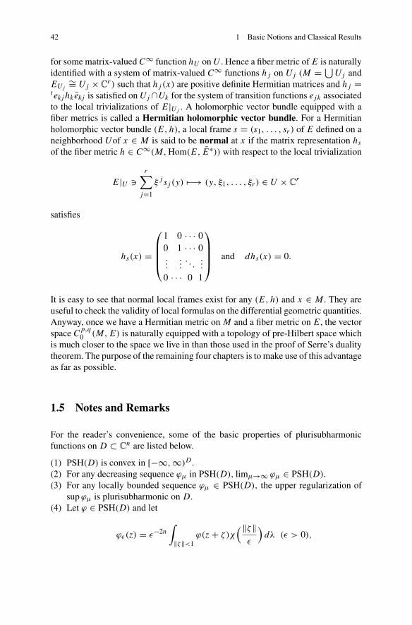
42 1 Basic Notions and Classical Results
for some matrix-valuedC∞ function hU onU . Hence a fiber metric ofE is naturallyidentified with a system of matrix-valued C∞ functions hj on Uj (M = ⋃Uj andEUj∼= Uj ×C
r ) such that hj (x) are positive definite Hermitian matrices and hj =t ekj hkekj is satisfied on Uj ∩Uk for the system of transition functions ejk associatedto the local trivializations of E|Uj . A holomorphic vector bundle equipped with afiber metrics is called a Hermitian holomorphic vector bundle. For a Hermitianholomorphic vector bundle (E, h), a local frame s = (s1, . . . , sr ) of E defined on aneighborhood Uof x ∈ M is said to be normal at x if the matrix representation hsof the fiber metric h ∈ C∞(M,Hom(E, E∗)) with respect to the local trivialization
E|U �r∑
j=1
ξj sj (y) �−→ (y, ξ1, . . . , ξr ) ∈ U × Cr
satisfies
hs(x) =
⎛⎜⎜⎜⎝
1 0 · · · 00 1 · · · 0...
.... . .
...
0 · · · 0 1
⎞⎟⎟⎟⎠ and dhs(x) = 0.
It is easy to see that normal local frames exist for any (E, h) and x ∈ M . They areuseful to check the validity of local formulas on the differential geometric quantities.Anyway, once we have a Hermitian metric on M and a fiber metric on E, the vectorspace Cp,q
0 (M,E) is naturally equipped with a topology of pre-Hilbert space whichis much closer to the space we live in than those used in the proof of Serre’s dualitytheorem. The purpose of the remaining four chapters is to make use of this advantageas far as possible.
1.5 Notes and Remarks
For the reader’s convenience, some of the basic properties of plurisubharmonicfunctions on D ⊂ C
n are listed below.
(1) PSH(D) is convex in [−∞,∞)D .(2) For any decreasing sequence ϕμ in PSH(D), limμ→∞ ϕμ ∈ PSH(D).(3) For any locally bounded sequence ϕμ ∈ PSH(D), the upper regularization of
supϕμ is plurisubharmonic on D.(4) Let ϕ ∈ PSH(D) and let
ϕε(z) = ε−2n∫‖ζ‖<1
ϕ(z+ ζ )χ(‖ζ‖
ε
)dλ (ε > 0),
1.5 Notes and Remarks 43
where χ is a C∞ nonnegative function on R with suppχ ⊂ (−∞, 1] and
∫Cn
χ(‖ζ‖) dλ = 1.
Then ϕε ∈ PSH(Dε), where Dε = {z ∈ D; dist(x,Cn \ D) > ε}, and ϕε ↘ ϕ asε → 0.
(5) Let D ⊂ Cn be a domain of holomorphy, let D ∩ {zn = 0} = D′ × {0} and let
δ : D′ → (0,∞) be defined by
δ(z′) = sup {r; {z′} × B1(0, r) ⊂ D} (z′ = (z1, . . . , zn−1)).
Then − log δ(z′) ∈ PSH(D′) (Oka’s lemma, substantially).The notion of plurisubharmonic function was introduced independently by
Lelong [Ll’42] and Oka [O-1]. For any hypersurface S ⊂ Cn, one can find
F ∈ O(Cn) such that i2π ∂∂ log |F | is identical as a (1,1)-current defined by
u �−→∫Sreg
u (u ∈ Cn−1,n−10 (Cn)).
This correspondence is often written as [S] = i2π ∂∂ log |F | and referred to as
Poincaré–Lelong formula. F satisfies the formula whenever F is locally a minimallocal defining function of S.
Holomorphic convexity of a complex space X is equivalent to saying that everycompact subset K ⊂ X has a compact holomorphic hull K defined by
K = {x ∈ X; |f (x)| ≤ supK
|f | for all f ∈ O(X)}.
Cartan and Thullen [C-T] introduced the notion of holomorphic convexity in thisform.
By this alternate definition, it is easy to see that X is holomorphically convexif and only if one can find for any unbounded sequence xμ(μ = 1, 2, . . . ) somef ∈ O(X) satisfying limμ→∞ sup |f (xμ)| = ∞.
Theorem 1.8 was first due to Skoda [Sk-2]. It was generalized by Yoshioka[Y’81] as follows.
Theorem 1.34 LetA be an analytic set of dimension≤ n−1 in an open setD ⊂ Cn
and let u ∈ Lp,q
(2),loc(D) (see Sect. 2.2.5 for the notation). If ∂u = 0 is satisfied on
D \ A in distribution sense (cf. Theorem 1.2), then ∂u = 0 holds on D.
The proof is straightforward from the definition of ∂u as a distribution. Skoda’soriginal proof was based on the Laurent expansion.
Let D be a domain in a complex manifold. If ∂D is strongly pseudoconvex atx, then one can find a local coordinate z = (z1, . . . , zn) around x such that ∂D isdefined by an equation of the form

44 1 Basic Notions and Classical Results
Re z1 = (Im z1)2 + |z2|2 + · · · + |zn|2 +O(2)
on a neighborhood of x. In particular, D is strictly convex near x in this coordinatesystem. On the other hand, weakly pseudoconvex domains are not always convexi-fiable in this sense. For instance, it was shown in [K-N] that the domain
Ω ={z ∈ C
2;Re z2 + |z1|8 + 15
7|z1|2Re z6
1 < 0}
is pseudoconvex and (0,0) has no neighborhood in which there exists a hypersurfacethat contains (0,0) and does not intersect with Ω .
Theorem 1.16 on the embedding of real analytic manifolds was preceded byMorrey’s work [M’58], where the compact case had been settled by the L2 method.A real analytic manifold S embedded into its complexification S(C) has an obviousproperty that TS contains no nontrivial complex subspaces of TS(C). For anycomplex manifold M of dimension n, a submanifold N ⊂ M of real dimensionn is said to be totally real if
(TN,x ⊗ C) ∩ T 1,0M = {0}
holds for all x ∈ N . Weierstrass-type approximation theorems are known to holdon certain totally real submanifolds (cf. [H-W’68, Nm’76, W’09]). Furthermore, aconnection between complex analysis and Riemannian geometry is known in thiscontext. Morimoto and Nagano [M-N’63] studied the complexification of compactand simply connected Riemannian symmetric spaces of rank 1, generalizing theindentification between the tangent bundle of the sphere x2
1 + · · · + x2n = 1 in R
n
and the hypersurface z21+· · ·+z2
n = 1 in Cn. [M-N’63] was followed by a geometric
theory of complex Monge–Ampère equations [G-S’92, L-S’91, P-W’91].In a letter to Takagi, Oka wrote in 1943 that a new question on the locally
pseudoconvex ramified domains arose after the solution of the Levi problem. Themanuscript for the full solution of the Levi problem had already been written inJapanese. At this point, Cartan had started to study the ideals of holomorphicfunctions in [C’40] to which Oka showed a great concern. In [C’44] Cartan askedseveral basic questions. Although Oka had no chance to read it because of WWII, hesolved some of them and sent the manuscript in 1948 to Cartan via USA with helpof Yasuo Akizuki, Hideki Yukawa, Shizuo Kakutani and André Weil. It appeared inBull. Soc. Math. France with [C].
Grauert’s direct image theorem (Theorem 1.28) was preceded by a theorem ofGrothendieck in algebraic geometry as well as a theorem of Kodaira and Spencerin the deformation theory of complex structures. Basically it asserts the uppersemicontinuity of dimHp,q(Mt , Et ), where Mt = f−1(t) for a proper surjectiveholomorphic map f → D such that df is everywhere of maximal rank andEt = E|Mt for a holomorphic vector bundle E→ M .
As a consequence of Remmert’s proper mapping theorem, the following factor-ization theorem is obtained.

References 45
Theorem 1.35 (cf. [C’60]) For any holomorphically convex space X, there existsa Stein space Y and a proper surjective holomorphic map ϕ : X→ Y satisfying thefollowing properties:
(1) Fibers of ϕ are connected.(2) ϕ∗OX = OY .(3) For any Stein space Z and any holomorphic map σ : X → Z, there exists a
unique holomorphic map τ : Y → Z satisfying σ = τ ◦ ϕ.ϕ is called the Stein factorization of X and Y is called the Remmert reduction
of X.Theorem 1.35 is closely related to the quotients of group actions on complex spaces.
A complex space X is said to be (p, q)-convex-concave if there exists a C2
proper map ϕ : X → (−1,∞) and a compact set K ⊂ X such that on everyconnected component of X \ K , either ϕ is positive and p-convex or ϕ is negativeand q-convex. There is a generalization of Theorem 1.31 to (p, q)-convex-concavespaces. As an application of a finiteness theorem on (1,1)-convex-concave space,it is known that every irreducible (1,1)-convex-concave space of dimension ≥3 isembeddable as an open subset of a 1-convex space (cf. [R’65]).
Grauert’s method of the proof of Theorem 1.28 entails generalizations to non-proper maps whose fibers are (p, q)-convex-concave. Some of them play importantroles in the theory of modifications and deformations (cf. [F-K’72, K-S’71, L’73,Siu’70, Siu’72, F’82]). See Theorem 2.84 in Chap. 2, for instance.
Since coherent analytic sheaves over X are locally free on a dense open subset ofX, questions on the sheaves can be reduced to those on holomorphic vector bundlesin certain circumstances. For instance, by virtue of Hironaka’s desingularizationtheorem, any torsion free coherent analytic sheaf F → X can be pulled back bya modification f : X → X to a sheaf which becomes locally free after taking thequotient by the torsion subsheaf (cf. [R’68]).
For any holomorphic map f : X → Y and a coherent analytic sheafF → X, there exists a sequence of doubly indexed vector spaces startingfrom {Hj(X,Rkf∗F )}j,k which naturally approximates {Hq(X,F )}q≥0 (Leray’sspectral sequence). By virtue of Remmert’s reduction, combining Leray’s spec-tral sequence with Theorem 1.28 and Cartan’s theorem B, one can deduce thatHq(X,F ) are Hausdorff if X is holomorphically convex. On the other hand, itis known that some complex Lie groups have non-Hausdorff H 0,1 (cf. [Kz-2, Vo]).
References
[C’40] Cartan, H.: Sur les matrices holomorphes de n variables complexes. J. Math. PuresAppl. 19, 1–26 (1940)
[C’44] Cartan, H.: Idéaux de fonctions analytiques de n variables complexes. Ann. Sci. ÉcoleNorm. Super. (3) 61, 149–197 (1944)
[C’60] Cartan, H.: Quotients of complex analytic spaces. In: 1960 Contributions to FunctionTheory. International Colloquium on Function Theory, Bombay, pp. 1–15. TataInstitute of Fundamental Research, Bombay (1960)
46 1 Basic Notions and Classical Results
[F-K’72] Forster, O., Knorr, K.: Relativ-analytische Räume und die Kohärenz von Bildgarben.Invent. Math. 16, 113–160 (1972)
[F’17] Forstneric, F.: Stein Manifolds and Holomorphic Mappings. The Homotopy Principlein Complex Analysis, 2nd edn. Ergebnisse der Mathematik und ihrer Grenzgebiete.3. Folge. A Series of Modern Surveys in Mathematics [Results in Mathematics andRelated Areas. 3rd Series. A Series of Modern Surveys in Mathematics], 56, pp.xiv+562. Springer, Cham (2017)
[F’82] Fujiki, A.: A coherency theorem for direct images with proper supports in the case ofa 1-convex map. Publ. Res. Inst. Math. Sci. 18(2), 451–476 (31–56) (1982)
[G-S’92] Guillemin, V., Stenzel, M.: Grauert tubes and the homogeneous Monge-Ampèreequation. II. J. Diff. Geom. 35(3), 627–641 (1992)
[H-W’68] Hörmander, L., Wermer, J.: Uniform approximation on compact sets in Cn. Math.
Scand. 23, 5–21 (1968)[K-S’71] Knorr, K., Schneider, M.: Relativexzeptionelle analytische Mengen. Math. Ann. 193,
238–254 (1971)[Ll’42] Lelong, P.: Définition des fonctions plurisousharmoniques. C. R. Acad. Sci. Paris 215,
398–400 (1942)[L-S’91] Lempert, L., Szöke, R.: Global solutions of the homogeneous complex Monge-Ampre
equation and complex structures on the tangent bundle of Riemannian manifolds.Math. Ann. 290(4), 689–712 (1991)
[L’73] Ling, H.S.: Extending families of pseudoconcave complex spaces. Math. Ann. 204,13–48 (1973)
[M-N’63] Morimoto, A., Nagano, T.: On pseudo-conformal transformations of hypersurfaces. J.Math. Soc. Jpn. 15, 289–300 (1963)
[M’58] Morrey, C.: The analytic embedding of abstract real-analytic manifolds. Ann. Math.(2) 68, 159–201 (1958)
[Nm’76] Nunemacher, J.: Approximation theory on totally real submanifolds. Math. Ann. 224,129–141 (1976)
[P-W’91] Patrizio, G., Wong, P.M.: Stein manifolds with compact symmetric center. Math. Ann.289(3), 355–382 (1991)
[R’65] Rossi, H.: Attaching analytic spaces to an analytic space along a pseudoconcaveboundary. In: 1965 Proceedings of the Conference on Complex Analysis, Minneapo-lis, pp. 242–256. Springer, Berlin (1964)
[R’68] Rossi, H.: Picard variety of an isolated singular point. Rice Univ. Stud. 54(4), 63–73(1968)
[Siu’70] Siu, Y.-T.: The 1-convex generalization of Grauert’s direct image theorem. Math. Ann.190, 203–214 (1970/1971)
[Siu’72] Siu, Y.-T.: A pseudoconvex-pseudoconcave generalization of Grauert’s direct imagetheorem. Ann. Scuola Norm. Sup. Pisa (3) 26, 649–664 (1972)
[Siu’78] Siu, Y.-T.: Pseudoconvexity and the problem of Levi. Bull. Am. Math. Soc. 84, 481–512 (1978)
[W’09] Wold, E.F.: A counterexample to uniform approximation on totally real manifolds inC
3. Mich. Math. J. 58(2), 401–409 (2009)[Y’81] Yoshioka, T.: Cohomologie à estimation L2 avec poids plurisousharmoniques et
extension des fonctions holomorphes avec contrôle de la croissance. Osaka J. Math.19(4), 787–813 (1982)
Chapter 2Analyzing the L2 ∂-Cohomology
Abstract For the bundle-valued differential forms on complex manifolds, a methodof solving ∂-equations with a control of L2 norm is discussed. Basic results areexistence theorems for such solutions under curvature conditions. They are variantsof Kodaira’s cohomology vanishing theorem on compact Kähler manifolds, andformulated as vanishing theorems with L2 conditions. Some of these L2 vanishingtheorems are generalized to finite-dimensionality theorems under the assumptionson the bundle-convexity. Besides applications to holomorphic functions, extensionsof the Hodge theory to noncompact manifolds will also be discussed.
2.1 Orthogonal Decompositions in Hilbert Spaces
The method of orthogonal projection introduced by H. Weyl [Wy-1] was an inno-vation in potential theory in the sense that it provided a general method of solvingthe Laplace equations without appealing to the fundamental solutions. This methodhas developed into a basic existence theory which is useful in complex analysison complex manifolds. Its basic part can be stated in an abstract form that certaininequality implies the solvability of an equation with an estimate for the norms.
2.1.1 Basics on Closed Operators
Let Hj(j = 1, 2) be two Hilbert spaces. Unless stated otherwise, we shall onlyconsider complex Hilbert spaces. We shall denote by (·, ·)j and ‖ ‖j respectively theinner products and the norms ofHj . Later we shall use also the notations (·, ·)Hj
and‖ ‖Hj
. By a closed operator from H1 to H2, we mean a C-linear map T from a denselinear subspaceΩ ⊂ H1 toH2 whose graphGT = {(u, T u) ∈ H1×H2 ; u ∈ Ω} isclosed in H1×H2. Ω is called the domain of T and denoted by Dom T . The imageT (Ω) of T will be denoted by Im T unless it is confused with the “imaginary part”
© Springer Japan KK, part of Springer Nature 2018T. Ohsawa, L2 Approaches in Several Complex Variables, SpringerMonographs in Mathematics, https://doi.org/10.1007/978-4-431-56852-0_2
47
48 2 Analyzing the L2 ∂-Cohomology
of T . Accordingly, Im T stands for the closure of the image of T , and not for theconjugate of the imaginary part of T . The kernel {u; T u = 0} of T will be denotedby Ker T . Note that Ker T is closed since so is GT .
The adjoint of a closed operator T , denoted by T ∗, is by definition a closedoperator from H2 to H1 satisfying
GT ∗ = {(v,w) ∈ H2 ×H1; (v, T u)2 = (w, u)1 for all u ∈ Dom T }. (2.1)
Note that GT ∗ = GT ∗ because the right-hand side of (2.1) is (G−T )⊥, theorthogonal complement of G−T in H1 × H2, up to the exchange of components.That (v,w), (v,w′) ∈ GT ∗ implies w = w′ follows from Dom T = H1. Vice versa,that Dom T ∗ = H2 is because T is single-valued. Obviously T ∗∗ = T .
Proposition 2.1 Im T ⊥ = Ker T ∗.
Corollary 2.1 H2 = Im T ⊕ Ker T ∗.
Similarly, H1 = Im T ∗ ⊕ Ker T , for T ∗∗ = T .
2.1.2 Kodaira’s Decomposition Theorem and Hörmander’sLemma
Let Hj(j = 1, 2, 3) be three Hilbert spaces with norms ‖ ∗ ‖j . Let T be a closedoperator from H1 to H2, and let S be a closed operator from H2 to H3 satisfyingDom S ⊃ Im T and ST = 0. Then, by Proposition 2.1 one has
H2 = Im T ⊕ Ker T ∗ = Im S∗ ⊕ Ker S. (2.2)
Since ST = 0, Im T ⊂ Ker S so that Im T ⊂ Ker S. Similarly Im S∗ ⊂ Ker T ∗,since T ∗S∗ = 0 follows immediately from ST = 0. Hence Im T and Im S∗ areothorgonal to each other. Combining these one has the following decompositiontheorem first due to K. Kodaira [K-1, Theorem 5].
Theorem 2.1 H2 = Im T ⊕ Im S∗ ⊕ (Ker S ∩ Ker T ∗).
In order to analyze this decomposition more in detail, the following is of basicimportance.
Lemma 2.1 (cf. [Hö-2, Proof of Lemma 4.1.1]) Let v ∈ H2. Then v ∈ Im T if andonly if there exists a nonnegative number C such that
|(u, v)2| ≤ C‖T ∗u‖1 (2.3)
holds for any u ∈ Dom T ∗.Moreover, the infimum of suchC is min {‖w‖1; Tw = v}.
2.1 Orthogonal Decompositions in Hilbert Spaces 49
Proof If v = Tw for some w ∈ H1, |(u, v)2| = |(u, T w)2| = |(T ∗u,w)1| ≤‖T ∗u‖1 ·‖w‖1. Hence one may put C = ‖w‖1. Conversely, suppose that (2.3) holdsfor any u ∈ Dom T ∗. Then the correspondence u→ (u, v)2 induces a continuous Clinear map from Im T ∗ to C, and further, one from H1 by composing the orthogonalprojection H1 → Im T ∗. Therefore, there exists a w ∈ H1 such that w ∈ H1 suchthat ‖w‖1 ≤ C and (u, v)2 = (T ∗u,w)1 holds for any u ∈ Dom T ∗. ��Corollary 2.2 Ker S = Im T if and only if there exists a function C : Ker S →[0,∞) such that |(u, v)2| ≤ C(v)‖T ∗u‖1 holds for any u ∈ Dom T ∗ and v ∈ Ker S.
Corollary 2.3 Ker S = Im T if there exists a constant C > 0 such that
‖u‖2 ≤ C(‖T ∗u‖1 + ‖Su‖3) (2.4)
holds for any u ∈ Dom T ∗ ∩ Dom S.
Proof Suppose that (2.4) holds for any u ∈ Dom T ∗ ∩ Dom S and take any v ∈Ker S. Let u ∈ Dom T ∗ and let u = u1 + u2, u1 ∈ Ker S, u2 ∈ Im S∗ be theorthogonal decomposition. Then T ∗u = T ∗u1, and (u, v)2 = (u1, v)2 since u2⊥v.Hence |(u, v)2| = |(u1, v)2| ≤ C‖T ∗u1‖ · ‖v‖ = C‖T ∗u‖ · ‖v‖, so that v ∈ Im T
by Corollary 2.1. ��Extension of Corollary 2.3 to the following is immediate.
Theorem 2.2 H2 = Im T ⊕ Im S∗ ⊕ (Ker S ∩ Ker T ∗) if there exists a constantC > 0 such that (2.4) holds for any u ∈ Dom T ∗ ∩ Dom S ∩ (Ker S ∩ Ker T ∗)⊥.
The hypothesis of Theorem 2.2 is fulfilled in a situation naturally arising incertain existence questions in Sect. 1.5 above. To see this, the following will beapplied later.
Proposition 2.2 (cf. [Hö-1]) Assume that from every sequence uk ∈ Dom T ∗ ∩Dom S with ‖uk‖2 bounded and T ∗uk → 0 in H1, Suk → 0 in H3, one can selecta strongly convergent subsequence. Then (2.4) holds for some C > 0 and any u ∈Dom T ∗ ∩ Dom T ∗ ∩ Dom S ∩ (Ker S ∩ Ker T ∗)⊥, and Ker S ∩ Ker T ∗ is finitedimensional.
Proof By hypothesis the unit sphere in Ker S∩Ker T ∗ is compact, so Ker S∩Ker T ∗has to be finite dimensional. If (2.4) were not true for any C, one could choose asequence uk⊥Ker S ∩ Ker T ∗ such that ‖uk‖2 = 1, T ∗uk → 0 in H1 and Suk → 0in H3. Let u be a strong limit of the sequence uk , which exists by hypothesis. Then‖u‖2 = 1 and u is orthogonal to Ker S ∩Ker T ∗ ∩Ker T ∗ although T ∗u = Su = 0,so that u ∈ Ker S ∩ Ker T ∗. This contradiction proves (2.4). ��
The following is also applied later:
Theorem 2.3 (cf. Theorem 1.1.4 in [Hö-1]) Let F be a closed subspace of H2containing Im T . Assume that ‖u‖2 ≤ C(‖T ∗u‖1 + ‖Su‖3) holds for any u ∈Dom T ∗ ∩ Dom S ∩ F . Then:

50 2 Analyzing the L2 ∂-Cohomology
(i) For any v ∈ Ker S ∩ F one can find w ∈ Dom T such that Tw = v and‖w‖1 ≤ C‖v‖2.
(ii) For any w ∈ Im T ∗ one can find v ∈ Dom T ∗ such that T ∗v = w and ‖v‖2 ≤C‖w‖1.
Proof
(i) Let v ∈ Ker S ∩ F , let u ∈ Dom T ∗, and let u = u1 + u2 + u3, where u1 ∈Ker S ∩ F , u2 ∈ Ker S and u2⊥F , and u3⊥Ker S. Since Im T ⊂ F and u2⊥F ,u2⊥Im T so that u2 ∈ Ker T ∗. Moreover, u3 ∈ Im S∗ ⊂ Ker T ∗. Thereforeu2 + u3 ∈ Ker T ∗, so that u1 ∈ Dom T ∗, and
|(u, v)2| = |(u1, v)2| ≤ C‖T ∗u1‖1 · ‖v‖2 (2.5)
Hence we have |(u, v)2| ≤ C‖T ∗u‖1 · ‖v‖2 from (2.5). Therefore the linearfunctional u �→ (u, v)2 on Dom T ∗ is continuous in T ∗u, so that there existsw ∈ H1 such that ‖w‖1 ≤ C‖v‖2 and
(u, v)2 = (T ∗u,w)1
holds for every u ∈ Dom T ∗ so that v = Tw.(ii) Let w = T ∗v0 and v0 = v1 + v2, where v1⊥Ker T ∗ and v2 ∈ Ker T ∗. Then
v1 ∈ Im T so that v1 ∈ F . Hence v1 ∈ F ∩ Dom T ∗ ∩ Ker S so that
‖v1‖2 ≤ C‖T ∗v1‖ = C‖T ∗v0‖ = C‖w‖.
Thus it suffices to put v = v1. ��
2.1.3 Remarks on the Closedness
Let the situation be as above. A basic observation of meta-theoretical importance isthat Im T is closed if and only if T |(Ker T )⊥ is invertible. In other words the followingholds.
Proposition 2.3 The following are equivalent:
(i) Im T = Im T .(ii) There exists a constant C such that
‖u‖ ≤ C‖T u‖ holds for any u ∈ Dom T ∩ (Ker T )⊥.
Proof (ii) ⇒ (i) is obvious. (i) ⇒ (ii) follows from Banach’s open mappingtheorem, or closed graph theorem, or uniform boundedness theorem. ��
Combining Proposition 2.3 with Corollary 2.1 one has:

2.2 Vanishing Theorems 51
Theorem 2.4 The following are equivalent:
(i) Im T = Im T .(ii) Im T ∗ = Im T ∗.
Accordingly, Corollary 2.2 is also strengthened to the following.
Theorem 2.5 H2 = Im T ⊕ Im S∗ if and only if there exists a constant C such that(2.4) holds for any u ∈ Dom T ∗ ∩ Dom S.
Similarly, the converse of Theorem 2.2 also holds.Let us add one more remark which is not so often mentioned but seems to be
useful. For an application see Example 2.2 below. (See also [Oh-5].) The proof isleft to the reader as an exercise.
Proposition 2.4 Im T = Im T if dim Ker S/Im T <∞.
2.2 Vanishing Theorems
Solvability criteria for ∂-equations on complex manifolds are often described ascohomology vanishing theorems. In order to apply the abstract theory presentedin the previous section, it is necessary to know that certain inequality holds for thebundle-valued differential forms under some curvature condition. The first vanishingtheorem of this type was established by Kodaira [K-2] on compact Kähler manifoldsand substantially by Oka [O-1, O-4] on pseudoconvex Riemann domains over Cn.A vanishing theorem for L2 ∂-cohomology groups on complete Kähler manifoldsunifies Kodaira’s vanishing theorem and Cartan’s Theorem B on Stein spaces. Thisviewpoint was first presented in a paper of Andreotti and Vesentini [A-V-1] and latereffectively developed in [A-V-2]. Independently and more thoroughly, Hörmander[Hö-1] established the method of L2 estimates for the ∂-operator, extending also apreceding work of Morrey [Mry]. The advantage of this method is its flexibility inthe limiting procedures as in Theorems 2.14 and 2.16. The argument below is basedalso on the method of Andreotti and Vesentini. It will be refined in the next sectionto recover a finiteness theorem of Hörmander.
2.2.1 Metrics and L2 ∂-Cohomology
Let (M,ω) be a (not necessarily connected but pure dimensional) Hermitianmanifold of dimension n and let (E, h) be a Hermitian holomorphic vector bundleover M . In order to analyze the ∂-cohomology groups of (M,E), the metricstructure (ω, h) is useful. As before, we denote by Cp,q(M,E) the set of E-valuedC∞ (p, q)-forms on M and by Cp,q
0 (M,E) the subset of Cp,q(M,E) consisting ofcompactly supported forms.

52 2 Analyzing the L2 ∂-Cohomology
The pointwise length of u ∈ Cp,q(M,E) with respect to the fiber metric inducedby ω and h, measured by regarding u as a section of
∧p(T
1,0M )∗ ⊗∧q
(T0,1M )∗ ⊗E,
is denoted by |u|(= |u|ω,h). The pointwise inner product of u and v is denoted by〈u, v〉(= 〈u, v〉ω,h). Then the L2 norm of u denoted by ‖u‖h, or simply by ‖u‖, isdefined as the square root of the integral
∫M
|u|2ωn
n! , (2.6)
which is finite if u ∈ Cp,q
0 (M,E). The inner product of u and v associated to thenorm is denoted by (u, v)h. (u, v)h is
∫M
〈u, v〉ω,h ωn
n!or
1
2(‖u+ v‖2 − ‖u‖2 − ‖v‖2)− i
2(‖iu+ v‖2 − ‖u‖2 − ‖v‖2) (2.7)
by definition, but has an expression more convenient for computation. Namely,
(u, v)h =∫M
u ∧ h ∗ v(=∫M
h(u) ∧ ∗v). (2.8)
Here h is identified with a section of E∗ ⊗ E∗(∼= Hom(E, E∗) and ∗ is a mapfrom Cp,q(M,E) to Cn−q,n−p(M,E) induced from the unique isometric bundlemorphism ∗ between
∧r(T CM)∗ and
∧2n−r(T CM)∗ (r = p + q) that satisfies
e1 ∧ e2 ∧ · · · ∧ er ∧ ∗(e1 ∧ e2 ∧ · · · ∧ er) = |e1 ∧ e2 ∧ · · · ∧ er |2ωn/n! (2.9)
for all ej (1 ≤ j ≤ r) in a fiber of (T C
M)∗. The map ∗ is called Hodge’s star
operator. For simplicity we put ∗v = ∗v. Then ∗ is a map from Cp,q(M,E) toCn−p,n−q(M,E).
Example 2.1 For M = Cn and ω = i
2
∑nj=1 dzj ∧ dzj ,
∗(dzI ∧ dzJ ) = cIJ dzI ′ ∧ dzJ ′ , (2.10)
where I ′ and J ′ complement I and J , respectively, and cIJ = (−1)(n−p)q in22p+q−n,
where p = |I | and q = |J |.Let Lp,q(2) (M,E) be the completion of the pre-Hilbert space C
p,q
0 (M,E) with
respect to the L2 norm. By Lebesgue’s theory of integration, Lp,q(2) (M,E) isnaturally identified with a subset of E-valued (p, q)-forms with locally square
2.2 Vanishing Theorems 53
integrable (=L2loc) coefficients. Then every element f of L
p,q
(2) (M,E) is natu-
rally identified with a C-linear function on Cp,q
0 (M,E) by the inner product· → (·, f )h. For simplicity, ∂ will also stand for a densely defined map fromLp,q
(2) (M,E) to Lp,q+1(2) (M,E) whose domain of definition, denoted by Dom ∂ , is
{f ∈ Lp,q
(2) (M,E); ∂f ∈ Lp,q+1(2) (M,E)}, where ∂f is defined in the sense of
distribution for any f ∈ Lp,q(2) (M,E). In other words, ∂f is regarded as an element
of Cn−p,n−q−10 (M,E∗)∗ by the equality
∫M
∂f ∧ v(= ∂f (v)) = (−1)p+q+1∫M
f ∧ ∂v
for all v ∈ Cn−p,n−q−10 (M,E∗), (2.11)
and “∂f ∈ Lp,q+1(2) (M,E)” means that there exists a unique element w ∈
Lp,q+1(2) (M,E) such that
∫Mw ∧ v = (−1)p+q+1
∫Mf ∧ ∂v holds for any v ∈
Cn−p,n−q−10 (M,E∗).
We define the L2 ∂-cohomology groups Hp,q
(2) (M,E) by
Hp,q
(2) (M,E) := Ker ∂ ∩ Lp,q(2) (M,E)/Im ∂ ∩ Lp,q(2) (M,E). (2.12)
Lp,q
(2) (M,E) and Hp,q
(2) (M,E) will be denoted by Lp,q
(2) (M,E,ω, h) and
Hp,q
(2) (M,E,ω, h), respectively, whenever (ω, h) must be visible. L2 de Rhamcohomology groups Hr
(2)(M) are defined similarly with respect to the exterior
derivative instead of ∂ . ∂ is obviously a closed operator from Lp,q
(2) (M,E) to
Lp,q+1(2) (M,E) so that it has its adjoint. It will be denoted by ∂∗h , or more simply
by ∂∗. A basic fact is that Hp,q
(2) (M,E) ∼= Ker ∂ ∩ Ker ∂∗ ∩ Lp,q
(2) (M,E) if
Im ∂ ∩ Lp,q(2) (M,E) is closed (cf. Theorem 2.1).
Example 2.2 With respect to the Euclidean metric,
dimHp,q
(2) (Cn) =
{0 if q = 0 or q > n,
∞ otherwise,
for any n ∈ N.Indeed, Hp,0
(2) (Cn) = 0 follows from Cauchy’s estimate. That Hp,q
(2) (Cn) = 0 for
q > n is trivial. To see that dimHp,1(2) (C
n) = ∞, it suffices to apply Propositions 2.3
and 2.4, combining Hp,0(2) (C
n) = 0 with an obvious fact that one can find a sequence
uk ∈ Lp,0(2) (C
n) such that ‖uk‖ = 1 and ‖∂uk‖ → 0 as k → ∞. The infinitedimensionality for general q follows similarly. Namely, the non-Hausdorff property
54 2 Analyzing the L2 ∂-Cohomology
ofHp,q
(2) (Cn) for 2 ≤ q ≤ n follows from that there exists a sequence uk ∈ Cp,q
0 (Cn)
such that ∂∗uk(⊥Ker ∂) are of norm 1 but ‖∂ ∂∗uk‖ → 0 as k → ∞, which is alsoobvious as in the case q = 1.
To obtain more advanced results, one needs to find natural conditions on (ω, h)in order to apply abstract existence theorems in Sect. 2.1.2. An effective conditionacceptable in most cases is the completeness of ω which guarantees in particular thedensity of Cp,q
0 (M,E) in Dom ∂∗ ∩ Lp,q(2) (M,E) with respect to the graph norm of
∂∗, which will be explained below.
2.2.2 Complete Metrics and Gaffney’s Theorem
A Hermitian manifold (M,ω) is said to be complete if M is complete as a metricspace with respect to the distance associated to ω. Recall that the distance betweenx, y ∈ M with respect to ω is defined as the infimum of
∫ 10
√γ ∗g where g is the
fiber metric of T 1,0M associated to ω regarded as a section of (T 1,0
M )∗ ⊗ (T0,1M )∗ and
γ runs through C∞ maps from [0,1] to M satisfying γ (0) = x and γ (1) = y. Thisdistance will be denoted by distω(x, y), or simply by d(x, y).
Example 2.3 (Cn, i2∑
dzj ∧ dzj ) is complete.
Proposition 2.5 (M,ω) is complete if and only if {y; d(x, y) < R} is relativelycompact for any x ∈ M and R > 0.
Proof The “if” part is obvious. The converse is easy to see from the Bolzano–Weierstrass theorem. ��
Since d(x, y) is Lipschitz continuous on M × M , it can be approximateduniformly by a C∞ function, say d(x, y) with bounded gradient. Let us fix a pointx0 ∈ M and put ρ(x) = d(x0, x). Let χ : R → [0,∞) be a C∞ function suchthat
(i) χ |(−∞, 1) ≡ 1
and
(ii) suppχ ⊂ (−∞, 2].Then we put χR(x) = χ(
ρ(x)R) for R > 1. An important property of χR is that
|dχR| ≤ C/R holds for some C > 0.
Proposition 2.6 Let (M,ω) be a Hermitian manifold and let (E, h) be a Hermitianholomorphic vector bundle over M . Then, for any u ∈ Dom ∂∩Lp,q(2) (M,E), χRu ∈Dom ∂ ∩ Lp,q(2) (M,E) and ‖χRu− u‖ + ‖∂(χRu)− ∂u‖ → 0 as R→∞.
2.2 Vanishing Theorems 55
Proof That ∂(χRu) = ∂χR∧u+χR∂u ∈ Lp,q+1(2) (M,E) and limR→∞ ‖χRu−u‖ =
0 is obvious. In order to see that limR→∞ ‖∂(χRu)− ∂u‖ = 0, it suffices to combinelimR→∞ ‖χR∂u− ∂u‖ = 0 and limR→∞(supM |∂χR|) = 0. ��
If (M,ω) is complete, supp(χRu) � M for all R. Hence there exists for each Ra sequence uk ∈ C
p,q
0 (M,E) satisfying ‖uk − χRu‖ + ‖∂uk − ∂(χRu)‖ → 0 ask→∞. Combining this observation with Proposition 2.6, we have:
Proposition 2.7 Let (M,ω) be a complete Hermitian manifold and let (E, h) be aHermitian holomorphic vector bundle over M . Then Cp,q
0 (M,E) is dense in Dom ∂
with respect to the norm ‖u‖ + ‖∂u‖.Similarly, since ∂∗ acts on Cp,q+1
0 (M,E) as a differential operator −∗h−1∂h∗,
which is easy to see from the Stokes’ formula and ∗ ∗ u = (−1)deg uu, Propo-sition 2.7 can be extended to the following important result which is first due toGaffney [Ga] for the exterior derivative d and formulated for ∂ by Andreotti andVesentini in [A-V-1, A-V-2].
Theorem 2.6 In the situation of Proposition 2.7, Cp,q
0 (M,E) is dense in Dom ∂ ∩Dom ∂∗ with respect to the norm ‖u‖ + ‖∂u‖ + ‖∂∗u‖.
The importance of Theorem 2.6 for our purpose lies in that integration by parts isavailable without worrying about the boundary terms to obtain the estimates imply-ing the existence theorems. To proceed in this way, formulas in the C∞(M) algebraof operators on
⊕2np+q=0 C
p,q(M,E) are useful. They will be described next.
2.2.3 Some Commutator Relations
Before presenting formulas involving ∂ , let us prepare some abstract formalism. LetR be a commutative ring and let M be a graded R module, i.e. M is a direct sumof submodules say Mj (j ∈ Z). If u ∈ Mj − {0}, j is called the degree of u anddenoted by deg u. Let
Πk(M ) = {T ∈M M ; T (Mj ) ⊂Mj+k for all j}.
For any T ∈ Πk(M )− {0} we put deg T = k. Then⊕
k∈ZΠk(M ) is a graded leftR algebra whose product is defined by composition. Elements of
⋃k∈ZΠk(M ) are
said to be homogeneous. Given S ∈ Πk(M ) and T ∈ Π�(M ), we define the gradedcommutator of S and T by
[S, T ]gr = S ◦ T − (−1)deg S deg T T ◦ S, (2.13)
where we put deg 0 = 0. The following straightforward consequence of thedefinition is very important.

56 2 Analyzing the L2 ∂-Cohomology
Lemma 2.2 (Jacobi’s identity) For any homogeneous S, T ,U ∈ Π(M ),
[[S, T ]gr, U ]gr − [S, [T ,U ]gr]gr = (−1)deg S deg T+1[T , [S,U ]gr]gr. (2.14)
Now let (M,ω)(dimM ≥ 1) and (E, h) be as before and set R = C∞(M),M = ⊕2n
p+q=0 Cp,q(M,E) and Mj = ⊕p+q=j Cp,q(M,E). Then, with respect
to this natural grading, ∂ ∈ Π1(M ). We shall identify the elements of Cp,q(M,E)
with those in Πp+q(M ) by letting them act on M by exterior multiplication fromthe left-hand side. Given θ ∈ Cp,q(M), we define θ∗ ∈ Π−p−q(M ) by requiringthe equality 〈θ ∧ u, v〉 = 〈u, θ∗v〉 for the pointwise inner product 〈·, ·〉 = 〈·, ·〉h tohold for any u ∈ Cr,s(M,E) and v ∈ Cr+p,s+q(M,E). Since ω ∈ C1,1(M), ω∗ ∈Π−2(M ). We shall use the notationΛ forω∗ following [W-1, W-2] and [N-1]. Someformulas involving Λ are of special importance. They will be recalled below.
For the special case (M,ω) = (Cn, i2∑
dzj ∧ dzj ), it is easy to see that
Λ = 1
2i
∑(dzj )
∗(dzj )∗
and
[dzj ,Λ]gr = −i(dzj )∗(1 ≤ j ≤ n).
Since this formula can be applied pointwise, one has the following in general.
Lemma 2.3 For any θ ∈ C0,1(M), [θ,Λ]gr = −iθ∗.Proposition 2.8 For any σ, τ ∈ C0,1(M), [σ, τ ∗]gr + [σ ∗, τ ]gr = 0.
Proof Since τ ∗ = i[τ ,Λ]gr and σ ∗ = −i[σ,Λ]gr, one has [σ, τ ∗]gr + [σ ∗, τ ]gr =i[σ, [τ ,Λ]gr]gr + i[[σ,Λ]gr, τ ]gr = [i[σ, τ ]gr,Λ]gr = 0. ��Similarly, replacing θ by ∂ one has a useful expression for [∂, Λ]gr. To describe it,let us put
∂$ = −∗∂∗. (2.15)
Proposition 2.9 For any u ∈ Cp,q
0 (M) and v ∈ Cp+1,q (M),∫M∂u∧∗v = ∫
Mu∧
∗∂$v.
Proof∫M∂u ∧ ∗v = ∫
Md(u ∧ ∗v)−(−1)p+q
∫Mu ∧ d∗v = −(−1)deg v−1
∫Mu ∧ ∂∗v
= − ∫Mu ∧ ∗∗∂∗v = ∫
Mu ∧ ∗(−∗∂∗v). ��
Lemma 2.4 [∂, Λ]gr = i∂$ if dω = 0.
Proof Since ∂ and ∂$ are differential operators of the first order, it suffices to showthe assertion for the Euclidean case. In this situation, first note that for any u ∈C∞(Cn),

2.2 Vanishing Theorems 57
[∂, Λ]gr(u dzI ∧ dzJ ) = 1
i
∑j∈I
∂u
∂zjdz∗j (dzI ∧ dzJ ). (2.16)
Hence, if v ∈ C∞0 (Cn) and {j,K} = I ,
([∂, Λ]gr(u dzI ∧ dzJ ), v) = 1
i
∫Cn
n∑j=1
∂u
∂zjdz∗j (dzI ∧ dzJ ) ∧ ∗(v dzK ∧ dzJ )
= 1
i
∫Cn
∂u
∂zjv · in2
(dz1 ∧ · · · ∧ dzn ∧ dz1 ∧ · · · ∧ dzn)
= −1
i
∫Cn
u∂v
∂zjin
2(dz1 ∧ · · · ∧ dzn ∧ dz1 ∧ · · · ∧ dzn)
= i
∫Cn
u dzI ∧ dzJ ∧ ∗(∑ ∂v
∂zjdzj ∧ dzK ∧ dzJ
)
= i(u, ∂v)(= i(u, ∂v)ω).
Hence [∂, Λ]gr = i∂$. ��For the sake of consistency, we shall denote ∂∗ (resp. ∂∗h ) by ∂$(resp. ∂$h) when
it operates on Cp,q(M) (resp. Cp,q(M,E)) as a differential operator. Let ∂h =h−1 ◦ ∂ ◦ h. Then [∂, Λ]gr + i∂$ and [∂h,Λ]gr − i∂$h are operators of order zero.(For the explicit expressions of them, see [Dm-3] or [Oh-7].)
Proposition 2.10 [∂, ∂$]gr − [∂$, ∂]gr = 0 if dω = 0.
Proof Since ∂$ = −i[∂, Λ]gr and ∂$ = i[∂,Λ]gr, one has [∂, ∂$]gr − [∂$, ∂]gr =i[∂, [∂,Λ]gr]gr + i[[∂, Λ]gr, ∂]gr = i[[∂, ∂]gr,Λ]gr = 0. ��
We note that the above computation works to show also that [∂, ∂$h]gr −[∂$, ∂h]gr = i[[∂, ∂h]gr,Λ]gr if dω = 0, because ∂$h and ∂h coincide with ∂$ and ∂respectively at a point x ∈ M with respect to a normal frame of E around x. Thefirst-order terms in the Taylor expansion of the coefficients of the zero order termsof ∂h appear in [∂, ∂h]gr = Θh ∈ C1,1(M,Hom(E,E)). Identifying Θh naturallywith an element of Π2(M ), we have
Theorem 2.7 (Nakano’s identity) [∂, ∂$h]gr − [∂$, ∂h]gr = [iΘh,Λ]gr if dω = 0.
Similarly, combining Lemmas 2.3 and 2.4 we obtain:
Theorem 2.8 For any θ ∈ C0,1(M), [∂, θ∗]gr + [∂$, θ ]gr = [i∂θ,Λ]gr holds ifdω = 0.
As a remark, we note that Lemma 2.3, Proposition 2.8 and Theorem 2.8 canbe generalized to commutator relations for θ ∈ C0,1(M,Hom(E,E)) by lettingθ∗ = ∗θ∗ and θh = h−1 ◦ t θ ◦ h as follows.
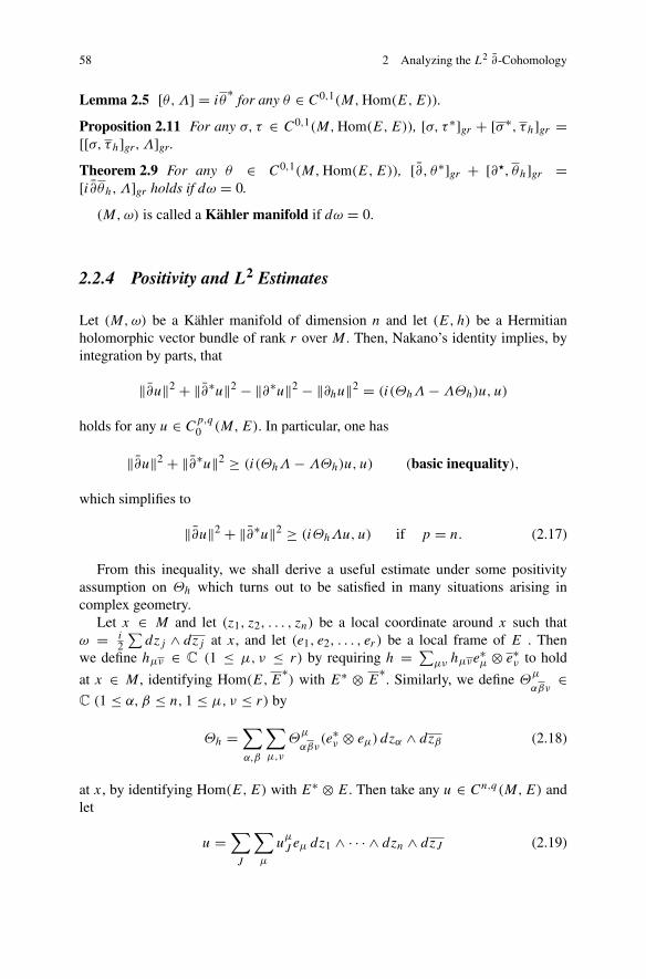
58 2 Analyzing the L2 ∂-Cohomology
Lemma 2.5 [θ,Λ] = iθ∗
for any θ ∈ C0,1(M,Hom(E,E)).
Proposition 2.11 For any σ, τ ∈ C0,1(M,Hom(E,E)), [σ, τ ∗]gr + [σ ∗, τh]gr =[[σ, τh]gr,Λ]gr.
Theorem 2.9 For any θ ∈ C0,1(M,Hom(E,E)), [∂, θ∗]gr + [∂$, θh]gr =[i∂θh,Λ]gr holds if dω = 0.
(M,ω) is called a Kähler manifold if dω = 0.
2.2.4 Positivity and L2 Estimates
Let (M,ω) be a Kähler manifold of dimension n and let (E, h) be a Hermitianholomorphic vector bundle of rank r over M . Then, Nakano’s identity implies, byintegration by parts, that
‖∂u‖2 + ‖∂∗u‖2 − ‖∂∗u‖2 − ‖∂hu‖2 = (i(ΘhΛ−ΛΘh)u, u)
holds for any u ∈ Cp,q
0 (M,E). In particular, one has
‖∂u‖2 + ‖∂∗u‖2 ≥ (i(ΘhΛ−ΛΘh)u, u) (basic inequality),
which simplifies to
‖∂u‖2 + ‖∂∗u‖2 ≥ (iΘhΛu, u) if p = n. (2.17)
From this inequality, we shall derive a useful estimate under some positivityassumption on Θh which turns out to be satisfied in many situations arising incomplex geometry.
Let x ∈ M and let (z1, z2, . . . , zn) be a local coordinate around x such thatω = i
2
∑dzj ∧ dzj at x, and let (e1, e2, . . . , er ) be a local frame of E . Then
we define hμν ∈ C (1 ≤ μ, ν ≤ r) by requiring h = ∑μν hμνe∗μ ⊗ e∗ν to hold
at x ∈ M , identifying Hom(E,E∗) with E∗ ⊗ E
∗. Similarly, we define Θμ
αβν∈
C (1 ≤ α, β ≤ n, 1 ≤ μ, ν ≤ r) by
Θh =∑α,β
∑μ,ν
Θμ
αβν(e∗ν ⊗ eμ) dzα ∧ dzβ (2.18)
at x, by identifying Hom(E,E) with E∗ ⊗ E. Then take any u ∈ Cn,q(M,E) andlet
u =∑J
∑μ
uμJ eμ dz1 ∧ · · · ∧ dzn ∧ dzJ (2.19)

2.2 Vanishing Theorems 59
hold at x. Then |u|2 = 2n+q∑
J
∑μ,ν hμνu
μJ u
νJ and
〈iΘhΛu, u〉 = 2n+q∑K
∑α,β,ν,κ
∑μ
Θμ
αβνhμκu
ν{K,α}uκ{K,β} (2.20)
at x.Similarly,
〈iΛΘhu, u〉 = 2n+q∑L
∑α,β,ν,κ
∑μ
Θμ
αβνhμκu
νL\{α}uκL\{β} (2.21)
at x.Note that
∑(∑
μ Θμ
αβνhμκ)ξ
ανξβκ ((ξαν) ∈ Cnr ) gives a quadratic form on
the fibers of T 1,0M ⊗ E as x varies.
Definition 2.1 (E, h) is said to be Nakano positive (resp. Nakano semipositive)if the quadratic form
∑(∑
μ Θμ
αβνhμκ)ξ
ανξβκ is positive (resp. semipositive)
at every point of M . Nakano negativity and Nakano seminegativity are definedsimilarly.
In other words, a Hermitian holomorphic vector bundle E is said to be Nakano(semi-) positive if, for any point x0 ∈ M , there is a neighborhood U = U(x0)
with local coordinate z = (z1, . . . , zn) around x0 and a coordinate w =(w1, . . . , wr) on the fibers of V |U coming from a holomorphic trivialization suchthat:
(1) over U we have the representation of the fiber metric∑
μν hμν(z)wμwν ,(2) the matrix (hμν(x0)) is the unit matrix,(3) the total derivative dhμν(x0) = 0,
and
(4) the Hermitian form −∑ (∂2hμν(x0)/∂zα∂zβ)γμαγνβ is positive (semi-)definite.
In particular, for any Nakano semipositive bundle (E, h) and for any holomor-phic section s of E∗, it is easy to see that log ‖s‖h∗ ∈ PSH(M). Here h∗ denotes thedual of h.
We shall say that a holomorphic vector bundle E is Nakano (semi-)positive ifit admits a fiber metric whose curvature form is (semi-)positive in the sense ofDefinition 2.1. In accordance with the positivity of the Kähler form ω, Nakanopositivity (resp. semipositivity) of the curvature form Θh in the above sense willbe denoted by iΘh > 0 (resp. ≥ 0). By an abuse of language we shall callthe eigenvalues of Θh also those of iΘh. Nakano positive (resp. semipositive) linebundles are simply called positive (resp. semipositive) line bundles. The curvatureform of a positive line bundle is naturally identified with a Kähler metric.

60 2 Analyzing the L2 ∂-Cohomology
By Corollary 2.3 and the inequality (2.17), the equality (2.20) eventually impliesthe following.
Theorem 2.10 Let (M,ω) be a complete Kähler manifold and let (E, h) be aHermitian holomorphic vector bundle over M such that iΘh − c IdE ⊗ ω ≥ 0for some c > 0. Then
Hn,q
(2) (M,E) = 0 for all q > 0. (2.22)
Corollary 2.4 (Kodaira–Nakano vanishing theorem) If (M,ω) is a compactKähler manifold and (E, h) is a Nakano positive vector bundle over M ,
Hn,q(M,E) = 0 (or equivalently Hq(M,O(KM ⊗ E)) = 0 ) for all q > 0.(2.23)
Corollary 2.5 Positive line bundles over compact complex manifolds are ample.
Here, a holomorphic line bundle L → M is said to be ample if there existsm ∈ N such that Lm is very ample in the sense that there exist s0, s1, . . . , sN ∈H 0,0(M,Lm) such that the ratio (s0 : s1 : · · · : sN) maps M injectively to CP
N−1
as a (not necessarily locally closed for noncompact M) complex submanifold.Similarly, the inequality ‖∂u‖2 + ‖∂∗u‖2 ≥ (−iΛΘhu, u) for u ∈ C0,q
0 (M,E)
implies:
Theorem 2.11 Suppose that (M,ω) is a complete Kähler manifold and there existsa c > 0 such that iΘh + c IdE ⊗ ω ≤ 0. Then H 0,q
(2) (M,E) = 0 for all q < n.
Remark 2.1 The Kodaira–Nakano vanishing theorem was first established in [K-2]for line bundles. The curvature condition for vector bundles of higher rank wasintroduced in [N-1]. Theorem 2.10 is already sufficient for many purposes, forinstance to solve the classical existence problems (cf. [Hö-1]). The reason why itworks is that every holomorphic vector bundle over M is Nakano positive if Madmits a strictly plurisubharmonic exhaustion function. A celebrated applicationof Corollary 2.4 is Kodaira’s characterization of projective algebraic manifoldsby the existence of positive line bundles (cf. [K-2, K-3]). The point of thefollowing discussion is that there still remains room for quite a few refinementsof Theorem 2.10 which reveal deeper truth of holomorphic functions and complexmanifolds. So, instead of reviewing the well-known applications of Theorem 2.10,we shall push it a little bit further.
2.2.5 L2 Vanishing Theorems on Complete Kähler Manifolds
Let (M,ω) be a complete Kähler manifold of dimension n and let (B, a) be aHermitian holomorphic line bundle over M .

2.2 Vanishing Theorems 61
Theorem 2.12 (cf. [A-N] and [A-V-1]) If ω = iΘa , then Hp,q
(2) (M,B) = 0 for
p + q > n and Hp,q
(2) (M,B∗) = 0 for p + q < n.
Proof By (2.20) and (2.21) (or by direct computation), one has
〈(ωΛ−Λω)u, u〉 = (p + q − n)|u|2 (2.24)
for any u ∈ Cp,q(M,B), whence the conclusion follows similarly to Theorems 2.10and 2.11. ��Corollary 2.6 (Akizuki–Nakano vanishing theorem) Let M be a compact com-plex manifold of dimension n and B → M a holomorphic line bundle which admitsa fiber metric whose curvature form is positive. ThenHp,q(M,B) = 0 for p+q > n
and Hp,q(M,B∗) = 0 for p + q < n.
Example 2.4 M = CPn, B = O(1) and a is the dual of the fiber metric of O(−1)
induced by ‖ζ‖2 (ζ ∈ Cn+1).
The following is an immediate variant of Theorem 2.12. The proof is similar.
Theorem 2.13 If the eigenvalues λ1 ≤ · · · ≤ λn ofΘa with respect toω everywheresatisfy
λ1 + · · · + λp − λq+1 − · · · − λn (= λ1 + · · · + λq − λp+1 − · · · − λn) ≥ c
for some positive constant c, then Hp,q
(2) (M,B) = 0 and Hn−p,n−q(2) (M,B∗) = 0.
A refinement of Theorem 2.10 in another direction is:
Theorem 2.14 (cf. [Dm-2] and [Oh-2, Oh-8]) Let M be a complex manifold ofdimension n which admits a complete Kähler metric, and let (B, a) be a positiveline bundle over M . Then, for any Kähler metric ω on M satisfying ω ≤ iΘa ,H
n,q
(2) (M,B,ω, a) = 0 for q > 0. Moreover, for any v ∈ Ln,q(2) (M,B,ω, a) ∩Ker ∂ ,
one can find w ∈ Ln,q−1(2) (M,B,ω, a) ∩ Dom ∂ satisfying ∂w = v and ‖w‖2 ≤
q‖v‖2.
Proof Let v ∈ Ln,q(2) (M,B,ω, a) ∩ Ker ∂ . Taking any complete Kähler metric ω∞on M , let ωε = ω+ εω∞ for any ε ≥ 0, let 〈, 〉ε denote the pointwise inner productwith respect to ωε , let Λε denote the adjoint of ωε(= ωε∧) with respect to ωε , let
(, )ε =∫M〈, 〉ε ω
nε
n! and let ‖ · ‖2ε = (·, ·)ε . Then, for any u ∈ Cn,q
0 (M,B),
∣∣∣∫M
〈u, v〉ε ωnε
n!∣∣∣2≤(iΘaΛεu, u)ε((iΘaΛε)
−1v, v)ε (Cauchy–Schwarz inequality).
(2.25)
Let x ∈ M be any point. Let v =∑ vJ dz1 ∧ · · · ∧ dzn ∧ dzJ , ω = i2
∑dzj ∧ dzj
and ω∞ = i2
∑θj dzj ∧ dzj (θj > 0) at x.
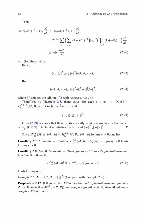
62 2 Analyzing the L2 ∂-Cohomology
Then
〈(iΘaΛε)−1v, v〉ε ω
nε
n! ≤ 〈(ωΛε)−1v, v〉ε ω
nε
n!= 2n+q
∑J
(∑j∈J
(1+ εθj )−1)|vJ |2
(∏j∈J
(1+ εθj )−1)ωnn!
≤ q|v|2ωn
n! (2.26)
at x (for almost all x).Hence
|(u, v)ε |2 ≤ q‖v‖2(iΘaΛεu, u)ε. (2.27)
But
(iΘaΛεu, u)ε ≤ ‖∂u‖2ε + ‖∂∗ε u‖2ε, (2.28)
where ∂∗ε denotes the adjoint of ∂ with respect to (ωε, a).Therefore, by Theorem 2.3, there exists for each ε a wε ∈ Dom ∂ ∩
Lp,q−1(2) (M,B,ωε, a) such that ∂wε = v and
‖wε‖2ε ≤ q‖v‖2. (2.29)
From (2.29) one sees that there exists a locally weakly convergent subsequenceof w 1
k(k ∈ N). The limit w satisfies ∂w = v and ‖w‖2 ≤ q‖v‖2. ��
Since Hn,q
(2) (M,B, iΘa, a) = Hn,q
(2) (M,B, ciΘa, a) for any c > 0, one has:
Corollary 2.7 In the above situation, Hn,q
(2) (M,B, ciΘa, a) = 0 for q > 0 holdsfor any c > 0.
Corollary 2.8 Let M be as above. Then, for any C∞ strictly plurisubharmonicfunction Φ : M → R,
Hn,q
(2) (M, i∂∂Φ, e−αΦ) = 0 for q > 0 (2.30)
holds for any α > 0.
Example 2.5 M = Cn,Φ = ‖z‖2. (Compare with Example 2.2.)
Proposition 2.12 If there exist a Kähler metric and a plurisubharmonic functionΦ on M such that Φ−1([−R,R]) are compact for all R ∈ R, then M admits acomplete Kähler metric.
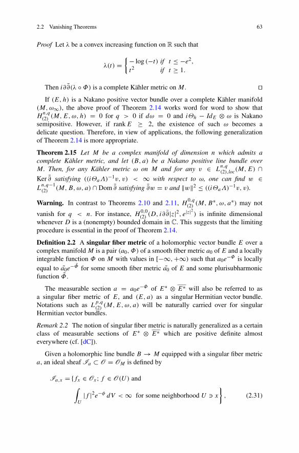
2.2 Vanishing Theorems 63
Proof Let λ be a convex increasing function on R such that
λ(t) ={− log (−t) if t ≤ −e2,
t2 if t ≥ 1.
Then i∂∂(λ ◦Φ) is a complete Kähler metric on M . ��If (E, h) is a Nakano positive vector bundle over a complete Kähler manifold
(M,ω∞), the above proof of Theorem 2.14 works word for word to show thatH
n,q
(2) (M,E,ω, h) = 0 for q > 0 if dω = 0 and iΘh − IdE ⊗ ω is Nakanosemipositive. However, if rankE ≥ 2, the existence of such ω becomes adelicate question. Therefore, in view of applications, the following generalizationof Theorem 2.14 is more appropriate.
Theorem 2.15 Let M be a complex manifold of dimension n which admits acomplete Kähler metric, and let (B, a) be a Nakano positive line bundle overM . Then, for any Kähler metric ω on M and for any v ∈ L
n,q
(2),loc(M,E) ∩Ker ∂ satisfying ((iΘaΛ)
−1v, v) < ∞ with respect to ω, one can find w ∈Ln,q−1(2) (M,B,ω, a) ∩ Dom ∂ satisfying ∂w = v and ‖w‖2 ≤ ((iΘaΛ)
−1v, v).
Warning. In contrast to Theorems 2.10 and 2.11, H 0,q(2) (M,B∗, ω, a∗) may not
vanish for q < n. For instance, H 0,0(2) (D, i∂∂|z|2, e|z|
2) is infinite dimensional
whenever D is a (nonempty) bounded domain in C. This suggests that the limitingprocedure is essential in the proof of Theorem 2.14.
Definition 2.2 A singular fiber metric of a holomorphic vector bundle E over acomplex manifold M is a pair (a0, Φ) of a smooth fiber metric a0 of E and a locallyintegrable function Φ on M with values in [−∞,+∞) such that a0e
−Φ is locallyequal to a0e
−Φ for some smooth fiber metric a0 of E and some plurisubharmonicfunction Φ.
The measurable section a = a0e−Φ of E∗ ⊗ E∗ will also be referred to as
a singular fiber metric of E, and (E, a) as a singular Hermitian vector bundle.Notations such as L
p,q
(2) (M,E,ω, a) will be naturally carried over for singularHermitian vector bundles.
Remark 2.2 The notion of singular fiber metric is naturally generalized as a certainclass of measurable sections of E∗ ⊗ E∗ which are positive definite almosteverywhere (cf. [dC]).
Given a holomorphic line bundle B → M equipped with a singular fiber metrica, an ideal sheaf Ia ⊂ O = OM is defined by
Ia,x ={fx ∈ Ox; f ∈ O(U) and∫U
|f |2e−φ dV <∞ for some neighborhood U � x}, (2.31)
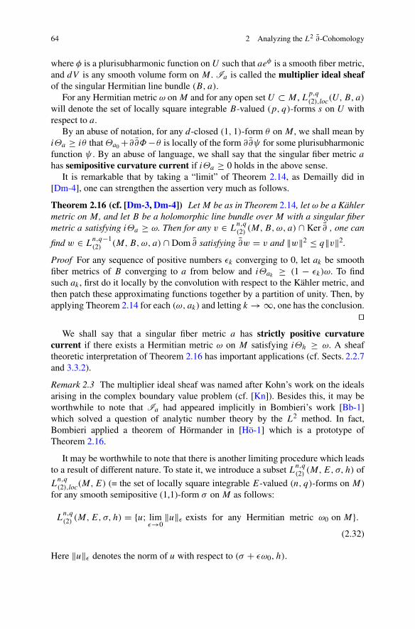
64 2 Analyzing the L2 ∂-Cohomology
where φ is a plurisubharmonic function on U such that aeφ is a smooth fiber metric,and dV is any smooth volume form on M . Ia is called the multiplier ideal sheafof the singular Hermitian line bundle (B, a).
For any Hermitian metric ω on M and for any open set U ⊂ M , Lp,q(2),loc(U,B, a)
will denote the set of locally square integrable B-valued (p, q)-forms s on U withrespect to a.
By an abuse of notation, for any d-closed (1, 1)-form θ on M , we shall mean byiΘa ≥ iθ that Θa0+∂∂Φ−θ is locally of the form ∂∂ψ for some plurisubharmonicfunction ψ . By an abuse of language, we shall say that the singular fiber metric ahas semipositive curvature current if iΘa ≥ 0 holds in the above sense.
It is remarkable that by taking a “limit” of Theorem 2.14, as Demailly did in[Dm-4], one can strengthen the assertion very much as follows.
Theorem 2.16 (cf. [Dm-3, Dm-4]) Let M be as in Theorem 2.14, let ω be a Kählermetric on M , and let B be a holomorphic line bundle over M with a singular fibermetric a satisfying iΘa ≥ ω. Then for any v ∈ Ln,q(2) (M,B,ω, a) ∩ Ker ∂ , one can
find w ∈ Ln,q−1(2) (M,B,ω, a) ∩ Dom ∂ satisfying ∂w = v and ‖w‖2 ≤ q‖v‖2.
Proof For any sequence of positive numbers εk converging to 0, let ak be smoothfiber metrics of B converging to a from below and iΘak ≥ (1 − εk)ω. To findsuch ak , first do it locally by the convolution with respect to the Kähler metric, andthen patch these approximating functions together by a partition of unity. Then, byapplying Theorem 2.14 for each (ω, ak) and letting k→∞, one has the conclusion.
��We shall say that a singular fiber metric a has strictly positive curvature
current if there exists a Hermitian metric ω on M satisfying iΘh ≥ ω. A sheaftheoretic interpretation of Theorem 2.16 has important applications (cf. Sects. 2.2.7and 3.3.2).
Remark 2.3 The multiplier ideal sheaf was named after Kohn’s work on the idealsarising in the complex boundary value problem (cf. [Kn]). Besides this, it may beworthwhile to note that Ia had appeared implicitly in Bombieri’s work [Bb-1]which solved a question of analytic number theory by the L2 method. In fact,Bombieri applied a theorem of Hörmander in [Hö-1] which is a prototype ofTheorem 2.16.
It may be worthwhile to note that there is another limiting procedure which leadsto a result of different nature. To state it, we introduce a subset Ln,q(2) (M,E, σ, h) of
Ln,q
(2),loc(M,E) (= the set of locally square integrable E-valued (n, q)-forms on M)for any smooth semipositive (1,1)-form σ on M as follows:
Ln,q
(2) (M,E, σ, h) = {u; limε→0‖u‖ε exists for any Hermitian metric ω0 on M}.
(2.32)
Here ‖u‖ε denotes the norm of u with respect to (σ + εω0, h).
2.2 Vanishing Theorems 65
Note that Ln,q(2) (M,E, σ, h) is a Hilbert space with norm ‖ · ‖σ = limε→0 ‖ · ‖εbecause of the monotonicity property “‖u‖ε ≤ ‖u‖ε′ if ε ≥ ε′”, so thatH
n,q
(2) (M,E, σ, h) and Hn,q
(2),loc(M,E, σ) are defined similarly.
Theorem 2.17 (cf. [Oh-8, Theorem 2.8]) Let M be a complex manifold of dimen-sion n admitting a complete Kähler metric, and let (E, h) be a Nakano semipositivevector bundle overM . Assume that σ is a smooth semipositive (1,1)-form onM suchthat dσ = 0 and iΘh−IdE⊗σ is Nakano semipositive. ThenHn,q
(2) (M,E, σ, h) = 0for q > 0.
Proof Let v ∈ Ln,q(2) (M,E, σ, h)∩Ker ∂ (q > 0), let ω0 be a complete Kähler metricon M and let Λε = (σ + εω0)
∗. Then
((IdE ⊗ εω0 + iΘh)Λε)−1v, v)ε ≤ ‖v‖2σ .
Hence one can find uε ∈ Ln,q−1(2) (M,E, σ +εω0, h) such that ∂uε = v and ‖uε‖ε ≤
‖v‖σ . Choosing a subsequence of uε as ε → 0 which is locally weakly convergent,we are done. ��Remark 2.4 The prototype of Theorem 2.17 is a vanishing theorem of Grauert andRiemenschneider in [Gra-Ri-1, Gra-Ri-2] which first generalized Kodaira–Nakano’svanishing theorem for semipositive bundles. In Sects. 2.2.7 and 2.3, more on theresults in this direction will be discussed.
As we have remarked in Sect. 2.2.1, Hn,q
(2) (M) may not vanish even if i∂∂Φ is a
complete metric (e.g. (M,ω) = (Cn, i∂∂‖z‖2) and 0 < q ≤ n). Nevertheless, ifadditionally the condition supM |dΦ| < ∞ is satisfied, a vanishing theorem holdsfor non-weighted L2 cohomology groups.
Theorem 2.18 (Donnelly–Fefferman vanishing theorem [D-F]) Let (M,ω) be acomplete Kähler manifold of dimension n. Assume that there exists a C∞ functionΦ : M → R such that ω = i∂∂Φ and supM |dΦ| < ∞. Then H
p,q
(2) (M) = 0 forp + q �= n.
Proof By Theorem 2.8, [∂, (∂Φ)∗]gr + [∂$, ∂Φ]gr = [i∂∂Φ,Λ]gr. Hence, combin-ing the assumption with (2.24) and the Cauchy–Schwarz inequality, one has
C(‖∂u‖ + ‖∂∗u‖ + ‖∂∗u‖ + ‖∂u‖)‖u‖ ≥ |p + q − n|‖u‖2 (2.33)
for any u ∈ Cp,q
0 (M). Here C = supM |∂Φ|. Since
‖∂u‖2 + ‖∂∗u‖2 = ‖∂u‖2 + ‖∂u‖2,
(2.33) implies an estimate equivalent to the assertion. ��Example 2.6 M = B
n,Φ = − log (1− ‖z‖2) (cf. Chap. 4).
66 2 Analyzing the L2 ∂-Cohomology
Example 2.7 M = Bn \ {0}, Φ = − log (− log ‖z‖2) (i∂∂Φ is the Poincaré metric
of D \ {0} if n = 1).
We shall say that a C∞ plurisubharmonic function Φ on M is of self boundedgradient, or of SBG for short, if
i(∂∂Φ − ε∂Φ ∧ ∂Φ) ≥ 0 for some ε > 0. (2.34)
Note that, if Φ is of SBG, then arctan (εΦ) is a bounded plurisubharmonic functionfor some ε > 0, which is strictly plurisubharmonic if so is Φ.
With this condition of SBG, a limiting process works similarly to the proof ofTheorem 2.14. For instance, one can deduce the following from Theorem 2.18.
Corollary 2.9 Let (M,ω) be a (not necessarily complete) Kähler manifold ofdimension n admitting a potential Φ of SBG. Assume that there exist an intervalI ⊂ R and a C∞ function λ : I → R such that Φ(M) ⊂ I , λ ◦ Φ is of SBG andsup ((λ′ + λ′′)/(λ′)2) <∞. Then Hp,q
(2) (M,ω) = 0 for p + q > n.
Example 2.8 M = {z; 0 < ‖z‖ < 1e}, Φ = −1
log ‖z‖ , I = (0, 1), λ(t) = − log t .
2.2.6 Pseudoconvex Cases
From the above-mentioned L2 vanishing theorems, we shall deduce here vanishingtheorems for the ordinary cohomology groups on pseudoconvex manifolds. First,vanishing theorems for positive bundles will be obtained from Theorems 2.12and 2.14. As before, let (M,ω) be a Kähler manifold of dimension n. Recall thatM is said to be pseudoconvex (resp. 1-complete) if M is equipped with a C∞plurisubharmonic (resp. strictly plurisubharmonic) exhaustion function. Pseudo-convex manifolds are also called weakly 1-complete manifolds (cf. [N-2, N-3]).Since every pseudoconvex Kähler manifold admits a complete Kähler metric byProposition 2.12, an immediate consequence of Theorem 2.12 is:
Theorem 2.19 (cf. [N-3]) Let M be a pseudoconvex manifold of dimension n andlet (B, a) be a positive line bundle over M . Then Hp,q(M,B) = 0 for p + q > n.
Proof Let p + q > n and v ∈ Lp,q
(2),loc(M,B) ∩ Ker ∂ . Then, it is easy to seethat for any smooth plurisubharmonic exhaustion function Φ on M , one can find aconvex increasing function λ such that v ∈ Lp,q(2) (M,B, iΘae−λ◦Φ , ae
−λ◦Φ). Hence,
v ∈ ∂(Lp,q−1(2),loc(M,B)) by Theorem 2.12. ��
Similarly, from Theorem 2.14 we obtain:
Theorem 2.20 (cf. [Kz-1]) Let M be a pseudoconvex manifold of dimension n andlet (E, h) be a Nakano positive vector bundle over M . Then Hn,q(M,E) = 0 forq > 0.

2.2 Vanishing Theorems 67
Proof Let q > 0 and v ∈ Ln,q
(2),loc(M,E) ∩ Ker ∂ . It is clear that for the Kählermetric iΘdeth there exists a smooth plurisubharmonic exhaustion function Φ on Msuch that ((iΘhe−ΦΛ)
−1v, v) < ∞ holds with respect to (iΘdeth, he−Φ). Hence
v ∈ Im ∂ by Theorem 2.14. ��Similarly, but using the L2 estimates for a sequence of solutions of the ∂-
equation, we have:
Theorem 2.21 Let M be a pseudoconvex manifold of dimension n and let (E, h)be a Nakano negative vector bundle over M . Then H 0,q
0 (M,E) = 0 for q < n.
On the other hand, by Serre’s duality theorem, Theorem 2.20 implies thefollowing.
Theorem 2.22 Under the situation of Theorem 2.20, H 0,q0 (M,E∗) = 0 for q < n.
Remark 2.5 Nakano positivity of E is not equivalent to Nakano negativity of E∗ ifrankE > 1 (cf. [Siu-5]).
Combining Theorems 2.20 and 2.21 (or 2.22), we obtain:
Theorem 2.23 Let M be a 1-complete manifold of dimension n. Then, for anyholomorphic vector bundle E over M , H 0,q (M,E) = 0 (resp. H 0,q
0 (M,E) = 0)holds for any q > 0 (resp. q < n).
Proof Since H 0,q (M,E) ∼= Hn,q(M, (KM)∗ ⊗ E) and (KM)
∗ ⊗ E is Nakanopositive by the 1-completeness of M , that H 0,q (M,E) = 0 holds for any q > 0follows from Theorem 2.20. The rest is similar. ��
Similarly to the above, one can remove the L2 condition at infinity fromTheorem 2.16. Since Theorem 2.16 can be applied for all Stein domains in M , theresult can be formulated in terms of the sheaf cohomology groups as in the spirit ofthe theorems of de Rham and Dolbeault. We shall summarize such interpretationsin the next subsection.
2.2.7 Sheaf Theoretic Interpretation
Let M be a complex manifold of dimension n and let (B, a) be a singular Hermitianline bundle over M . By W p,q(B, a) we shall denote a sheaf over M whose sectionsover an open set U ⊂ M are those elements of Lp,q(2),loc(U,B, a)(⊂ L
p,q
(2),loc(U,B))
whose images by ∂ (in the distribution sense) belong to Lp,q+1(2),loc(U,B, a). Then,
Theorem 2.16 implies that the complex (W n,q(B, a)q≥0, ∂) is a fine resolution ofthe sheaf O(KM)⊗Ia . Hence, as an immediate consequence of Theorem 2.16 weobtain:

68 2 Analyzing the L2 ∂-Cohomology
Theorem 2.24 (Nadel’s vanishing theorem, cf. [Nd]) In the situation of Theo-rem 2.16, assume moreover that M is pseudoconvex. Then
Hq(M,O(KM ⊗ B)⊗Ia) = 0
for q > 0.
Theorem 2.24 was proved for the compact case by Nadel [Nd] who applied itto prove the existence of Kähler–Einstein metrics on certain projective algebraicmanifolds. Nadel proved also the coherence of Ia (cf. Chap. 3).
As well as the generalization to noncompact manifolds, Nadel’s vanishingtheorem can be extended easily to complex spaces with singularities.
Definition 2.3 Given a reduced complex space X of pure dimension n, a sheaf ωXover X is called the L2-dualizing sheaf of X if
Γ (U,ωX) = {u ∈ Γ (U ∩Xreg,O(KXreg)); u ∈ Ln,0(2) (V ∩Xreg) for every V � U}
for any open subset U ⊂ X.
Similarly, for any singular Hermitian line bundle (B, a) over X, the multiplierdualizing sheaf ωX,a is defined as the collection of square integrable germs of B-valued holomorphic n-forms with respect to a.
For any desingularization π : X → X, one has ωX = π∗O(KX), since the
support of effective divisors are negligible as the singularities of L2 holomorphicfunctions (cf. Theorem 1.8). In particular, ωX is a coherent analytic sheaf over X.
Theorem 2.25 (Nadel’s vanishing theorem on complex spaces) Let X be areduced and pseudoconvex complex space of pure dimension n with a Kähler metric,and let (B, a) be a singular Hermitian line bundle over X with strictly positivecurvature current. Then
Hq(X,O(B)⊗ ωX,a) = 0
for q > 0.
Generally speaking, precise vanishing theorems are important in complex geom-etry not only because they yield effective results, but also because they give a widerperspective in the theory of symmetry and invariants. In fact, their generalizationsand variants have been found in the literature of geometry, analysis and algebra. Letus review an example of such a development motivated by more algebraic ideas.
Soon after the appearance of [Gra-Ri-1, Gra-Ri-2], Ramanujam [Rm-1] cameup with a similar generalization of Kodaira’s vanishing theorem. Ramanujam’sbackground was Grothendieck’s theory [Grt-1, Grt-2], which is a foundation ofalgebraic geometry over the fields of arbitrary characteristic. In this situation, hecould prove a vanishing theorem only for surfaces. No one could have done betterbecause it is false for higher dimensions in positive characteristic. Note that acounterexample to Kodaira’s vanishing theorem in positive characteristic was foundonly after the publication of [Rm-2] (cf. [Rn]). Anyway, from this new perspective,

2.2 Vanishing Theorems 69
inspired also by Bombieri’s work [Bb-2] on pluricanonical surfaces, he couldstrengthen the vanishing theorem in the following way.
Theorem 2.26 (cf. [Rm-2]) Let X be a nonsingular projective algebraic variety ofdimension n ≥ 2 over C and let L → X be a holomorphic line bundle whose firstChern class c1(L) satisfies c1(L)
2 > 0 and c1(L) · C (:= degL|Cred ) ≥ 0 for anycompact complex curve C in X. Then H 1(X,O(L∗)) = 0.
In the case where L = [D] for some effective divisor D on X, H 1(X,O(L∗)) = 0implies in particular that the support |D| of D is connected.
The formulation of Ramanujam’s theorem is in the same spirit as in Nakai’snumerical criterion for ampleness of line bundles (cf. [Na-1, Na-2, Na-3]). Mumford[Mm] gave an alternate proof of Theorem 2.26 but did not proceed to the higher-dimensional cases. Kawamata [Km-1] and Viehweg [V] overcame this shortcomingindependently by establishing the following:
Theorem 2.27 Let X be a nonsingular projective algebraic variety of dimension nand let L→ X be a holomorphic line bundle with c1(L)
n > 0 such that c1(L) ·C ≥0 for any compact complex curve C in X. Then
Hk(X,O(KX ⊗ L)) = 0
holds for all k > 0.
By the Serre duality, this contains Theorem 2.26 as a special case. Beinga numerical criterion for the cohomology vanishing, Theorem 2.27 is of basicimportance in birational geometry. (See [Km-M-M] for instance.) A simple analyticproof of Theorem 2.27 was later given by Demailly [Dm-4]. According to themodern terminology, L is said to be nef (= numerically effective or numericallyeventually free) if c1(L) · C ≥ 0 for any complex curve C on X. The notion ofnef line bundles naturally extends to Kähler manifolds. Namely, a holomorphic linebundle L over a compact Kähler manifold is called nef if c1(L) is in the closureof the cone of Kähler classes. Nef bundles over nonsingular projective varietiesare nef in the latter sense because any Kähler class is in the closure of the conegenerated over R+ by the first Chern classes of positive line bundles. Nef linebundles also make sense over the proper images of compact Kähler manifolds byalmost biholomorphic maps. Furthermore, in virtue of a theorem of Varouchas [Va],they can be defined similarly over proper holomorphic images of compact Kählermanifolds. Demailly and Peternell [Dm-P] proved:
Theorem 2.28 Let X be a compact and normal complex space of dimension nadmitting a Kähler metric, and let L be a nef line bundle over X with c1(L)
2 �= 0.Then Hq(X,O(KX ⊗ L)) = 0 f or q ≥ n− 1.
Similarly to Theorem 2.26, if n ≥ 2 and L = [D] for some effective divisor D,it follows from the assumption of Theorem 2.28 that |D| is connected. In [Oh-27]it is proved that H 1
0 (X \ |D|,O) = 0 under the same hypothesis. Recall that H 10
denotes the cohomology with compact support. A question was raised in [Dm-P-S]

70 2 Analyzing the L2 ∂-Cohomology
whether or not Hq(X,O(KX ⊗ L)) = 0 holds if L is nef and c1(L)n−q+1 �= 0. It
was recently settled by J.-Y. Cao [CJ].There exists another sheaf theoretic interpretation of Theorem 2.14, slightly
different from that of Theorem 2.16. It is based on an observation that,although L
n,q
(2) (M,E, σ, h) are subsets of Ln,q
(2),loc(M,E) for semipositive σ ,
Hn,q
(2),loc(M,E, σ) can be naturally isomorphic to certain sheaf cohomology groupon a quotient space of M . Assume that there exists a proper holomorphic map π
from M to a complex space X admitting a Kähler metric ω. Then, Theorem 2.14implies that Hn,q
(2),loc(M,E, π∗ω) ∼= Hq(X, π∗O(KM ⊗ E)) for q ≥ 0 if E is
Nakano semipositive on some neighborhood of π−1(x) for any x ∈ X. In particular,one has the following.
Theorem 2.29 (cf. [Oh-8, Theorem 3.1]) Let M be a pseudoconvex Kähler man-ifold, let X be a complex space with a Kähler metric ω, and let π : M → X be aproper holomorphic map. Then, for any Nakano semipositive vector bundle (E, h)over M satisfying iΘh − IdE ⊗ π∗ω ≥ 0, Hq(X, π∗O(KM ⊗ E)) = 0 for q > 0.
Remark 2.6 In [Oh-8], this was stated only for compact M . As in the case ofTheorem 2.25, Theorem 2.29 has several predecessors besides the Kodaira–Nakanovanishing theorem. These are semipositivity theorems for the direct image sheavesof the relative canonical bundles KM ⊗π∗K−1
X for Kählerian M and nonsingular X(cf. [Gri-1, Gri-3, F-1]). Quite recently, there was an unexpected development in thetheory of L2 holomorphic functions closely related to the semipositivity theorem ofthis type (see Chaps. 3 and 4). See [Ko’86-1, Ko’86-2] and [Ko’87] for the higherdirect images of KM ⊗ π∗K−1
X .
Roughly speaking, the choice of singular fiber metrics and degenerate basemetrics (=pseudometrics) amounts to the choice of boundary conditions in theproblems of partial differential equations. There are inductive arguments to produce“good” singular fiber metrics (cf. Lemma 3.2 in Chap. 3).
Concerning the L2 ∂-cohomology groups of type (p, q), there are resultswhich relate analytic invariants and topological invariants on complex spaces withsingularities. Let us review some of these results in the next subsection.
2.2.8 Application to the Cohomology of Complex Spaces
The symmetry [∂, ∂$]gr = [∂$, ∂]gr of the complex Laplacian on a compact Kählermanifold M yields Hodge’s decomposition theorem
Hr(M) ∼=⊕
p+q=rHp,q(M)
Hp,q(M) ∼= Hq,p(M)
(cf. [W]). Hence it is natural to expect that the corresponding decomposition forthe spaces of L2 harmonic forms carries similar geometric information also on

2.2 Vanishing Theorems 71
some noncompact Kähler manifolds. Grauert [Gra-2] has shown that, for everycompact Kähler space X, Xreg carries a complete Kähler metric. Based on this, itwill be shown below after [Sap] and [Oh-10, Oh-11, Oh-14] that the L2 cohomologygroups of Xreg with respect to some class of (not necessarily complete) metrics arecanonically isomorphic to the ordinary ones in certain degrees. Accordingly, theHodge decomposition remains true for M = Xreg there. The method also gives apartial solution to a conjecture of Cheeger, Goresky and MacPherson in [C-G-M].Related results are also reviewed.
Let X be a (reduced) complex space. A Hermitian metric on X is defined as aHermitian metric or a positive (1,1)-form say ω onXreg, such that, for any point x0 ∈SingX there exists a neighborhood U � x0 in X, a proper holomorphic embeddingι of U into a polydisc DN for some N and a C∞ positive (1, 1) form Ω on D
N suchthat ω = ι∗Ω holds on U ∩ Xreg. A complex space X equipped with a Hermitianmetric is called a Hermitian complex space. A Hermitian complex space (X, ω) iscalled a Kähler space if dω = 0.
Lemma 2.6 Let (X, ω) be a compact Kähler space. Then there exists a continuousfunction ϕ : X→ [0, 1] such that ω+ i∂∂ϕ is a complete Kähler metric on Xreg forwhich the length of ∂ϕ is bounded.
Proof Let x0 ∈ SingX be any point and let f1, . . . , fm be holomorphic functionson a neighborhood U of x0 which generate the ideal sheaf ISingX on U . Then, byshrinking U if necessary so that
∑mj=1 |fj |2 < e−e on U , we put
ϕU = 1
log (− log∑m
j=1 |fj |2).
By an abuse of notation, we put ϕU = 1 if U ∩ SingX = ∅. In order tosee that a desired function ϕ can be obtained by patching ϕU by a partition ofunity, let us take another generator (g1, . . . , g�) of ISingX over U . Then it is easyto verify that one can find a neighborhood V � x0 such that ω + i∂∂ϕU andω + i∂∂(log (− log
∑�k=1 |gk|2))−1 are positive and quasi-isometrically equivalent
to each other on Xreg∩V . Moreover, it is also immediate that, for any ε > 0 one canfind a neighborhood W � x0 such that the length of ∂ϕU on W ∩ Xregwith respectto ω + i∂∂ϕU (or even with respect to i∂∂ϕU ) is less than ε.
Now let U = {Uα}α∈A be a finite open cover of X by such U , and let ρα be aC∞ partition of unity associated to U . We put
ϕ =∑α∈A
ραϕUα . (2.35)
Then ϕ is a continuous function on X with values in [0, 1] such that ϕ−1(0) =SingX and ϕ|Xreg is C∞. Furthermore, since ∂(
∑ρα) = 0 and ∂∂(
∑ρα) = 0,
∂∂ϕ =∑
∂∂ρα(ϕUα − ϕUβ )+∑
∂ρα(∂ϕUα − ∂ϕUβ )
+∑
(∂ϕUα − ∂ϕUβ )∂ρα +∑
ρα∂∂ϕUα . (2.36)

72 2 Analyzing the L2 ∂-Cohomology
Combining (2.34) with the above remarks on ω + i∂∂ϕU and ∂ϕU , it is clear thatω + εi∂∂ϕ is a complete Kähler metric on Xreg for 0 < ε � 1. ��
Any function ϕ of the form (2.35) will be called a Grauert potential on X. Ametric of the form ω+i∂∂ϕ will then be called a Grauert metric. The boundednesscondition for ∂ϕ is important when one wants to extend the Hodge theory tocomplex spaces with singularities. A basic fact for that is the following:
Proposition 2.13 Let (M,ω) be a complete Kähler manifold, let (E, h) be aHermitian holomorphic vector bundle over M and let ϕ be a real-valued boundedC∞ function on M such that ∂ϕ is bounded with respect to ω. Then, for anynonnegative integers p and q, and for any u ∈ Lp,q(2) (M.E) satisfying u ∈ Dom ∂ ∩Dom ∂∗, u belongs to the domain of the adjoint of ∂ with respect to the modifiedfiber metric he−ϕ . If moreover Θh and ∂∂ϕ are also bounded, u belongs also to thedomains of ∂h, ∂he−ϕ and ∂
$.
Proof The proof of the first assertion follows immediately from the definition of theadjoint of ∂ . The second assertion follows from Nakano’s identity. ��
For any open set U ⊂ X, the L2 cohomology groups Hp,q
(2) (U ∩Xreg),Hr(2)(U ∩
Xreg) with respect to ω will be denoted by Hp,q
(2) (U),Hr(2)(U), for simplicity. The
L2 cohomology groups with supports restricted to relatively compact subsets ofU will be denoted by H
p,q
(2),0(U),Hr(2),0(U). Similarly, the L2 cohomology groups
with respect to a Grauert metric ω + i∂∂ϕ and those with “compact support inU” will be denoted by H
p,q
(2),ϕ(U),Hr(2),ϕ(U),H
p,q
(2),ϕ,0(U) and Hr(2),ϕ,0(U). Then
the vanishing of the L2 cohomology of Akizuki–Nakano type on complete Kählermanifolds implies that these L2 cohomology groups do not see the singularities inhigher degrees. For instance the following holds.
Theorem 2.30 Let (X, ω) be a compact Kähler space of pure dimension n and letϕ be a Grauert potential on X. If dim SingX = 0, then
Hp,q
(2) (X)∼= H
p,q
(2),ϕ(X)∼= H
p,q
0 (Xreg) for p + q > n+ 1
and
Hr(2)(X)
∼= Hr(2),ϕ(X)
∼= Hr0 (Xreg) for r > n+ 1.
Moreover, the natural homomorphisms from Hp,q
0 (Xreg) to Hp,q
(2) (X) and Hp,q
(2),ϕ(X)
are surjective for p + q = n + 1, and so are those from Hn+10 (Xreg) to Hn+1
(2) (X)
and Hn+1(2),ϕ(X).
Proof Let x0 ∈ SingX and let W � {x0} be a neighborhood such that W ∩SingX ={x0}. Let δ > 0 be sufficiently small so that Wδ := {x ∈ W ;ϕ(x) < δ} � W .Then, with respect to the complete Kähler metric ωε,δ := ω + εi∂∂(log (δ − ϕ))−1
(0 < ε � δ < 1) on Wδ \ {x0}, the L2 cohomology groups Hp,q
(2) (Wδ \ {x0}, ωε,δ)
2.2 Vanishing Theorems 73
vanish for p + q > n by Theorem 2.12. On the other hand, it is easy to see that, forany L2 (p, q) form f on Wreg with p+q > n, f |Wreg\{x0} is L2 with respect to ωε,δ .Therefore the natural homomorphism
Hp,q
0 (Xreg) −→ Hp,q
(2),ϕ(X)
is surjective if p + q > n and injective if p + q > n + 1. Concerning the L2 deRham cohomology groups Hr
(2), that Hr(2)(Wδ \ {x0}, ωε,δ) vanish for r > n can be
shown as follows: Let u ∈ Lr(2)(Wδ \ {x0}, ωε,δ), du = 0 and r > n. Then u is
decomposed as u = ur,0 + ur−1,1 + · · · + u0,r with up,q ∈ Lp,q(2) (Wδ \ {x0}, ωε,δ).Since du = 0, ∂u0,r = 0, so that there exists v ∈ L
0,r−1(2) (Wδ \ {x0}, ωε,δ) such
that ∂v = u0,r and ∂∗v = 0. By Proposition 2.13, it follows in particular that∂v ∈ L
1,r−1(2) (Wδ \ {x0}, ωε,δ). Hence u − dv ∈ ⊕r
j=1 Lj,r−j(2) (Wδ \ {x0}, ωε,δ).
Proceeding similarly, we obtain that the L2 de Rham cohomology class of u is 0.Thus we obtain the assertion for Hp,q
(2),ϕ(X) and Hr(2),ϕ(X). As for the ordinary L2
cohomology groups Hp,q
(2) (X) and Hr(2)(X), they are considered respectively as the
limits of Hp,q
(2),ϕ(X) and Hr(2),ϕ(X). For that, we make a special choice of ϕ as in
the proof of Lemma 2.6. Then, after fixing δ, we consider ω as the limit of ωε,δ(ε → 0). Then, as is easily checked, Lp,q(2) (Wδ \ {x0}, ω) ⊂ L
p,q
(2) (Wδ \ {x0}, ωε,δ)if p + q > n, so that by solving the ∂ equation ∂vε = u with L2 norm estimatesfor vε ∈ L
p,q−1(2) (Wδ \ {x0}, ωε,δ) uniformly in ε, and by taking the weak limit of
a subsequence of vε , we obtain the required the vanishing results for Hp,q
(2) (Wδ \{x0}, ω) as well as those for Hr
(2)(Wδ \ {x0}, ω). ��In view of the long exact sequences
· · · −→ Hp,q
0 (Xreg) −→ Hp,q
(2) (X)
−→ lim−→Hp,q
(2) (X \K) −→ Hp,q+10 (Xreg) −→ · · ·
(resp. · · · −→ Hp,q
0 (Xreg) −→ Hp,q
(2),ϕ(X) −→ lim−→Hp,q
(2),ϕ(X \K)−→ H
p,q+10 (Xreg) −→ · · · ),
where lim−→ denotes the inductive limit of the system
Hp,q
(2) (X \K1) −→ Hp,q
(2) (X \K2)
(resp. Hp,q
(2),ϕ(X \K1) −→ Hp,q
(2),ϕ(X \K2)) (K1 ⊂ K2 � Xreg),
Theorem 2.30 says
lim−→Hp,q
(2) (X \K) = lim−→Hp,q
(2),ϕ(X \K) = 0 if p + q > n. (2.37)
74 2 Analyzing the L2 ∂-Cohomology
The proof shows that
lim−→Hr(2)(X \K) = lim−→Hr
(2),ϕ(X \K) = 0 for r > n
is a consequence of (2.37). Existence of the natural homomorphisms
lim−→Hp,q
(2),ϕ(X \K) = lim−→Hp,q
(2) (X \K), p + q > n
is crucial to deduce
lim−→Hp,q
(2) (X \K) = 0
from
lim−→Hp,q
(2),ϕ(X \K) = 0.
The Kähler condition is superfluous here. Obviously Theorem 2.30 holds forcompact Hermitian complex spaces. Thus, an essential part of Theorem 2.30 canbe stated as a Dolbeaut-type lemma:
Lemma 2.7 Let V be an analytic set of pure dimension n in DN containing z0 as an
isolated singularity. Then there exists a neighborhood U � z0 such that Hp,q
(2) (U) =0, Hp,q
(2),ϕ(U) = 0 for p + q > n and Hr(2)(U) = 0, Hr
(2),ϕ(U) = 0 for r > n.
Because of the presence of singularities, it is not allowed immediately to applythe ordinary duality theorems due to Poincaré and Serre to obtain the results forp + q, r < n, simply reversing the direction of the arrows. Nevertheless there is amethod to prove the following (see [Oh-10, Supplement]).
Lemma 2.8 Let V and z0 be as above. Then there exists a neighborhood U � z0such that
Hp,q
(2),0(U) = 0, Hp,q
(2),ϕ,0(U) = 0 for p + q < n,
and
Hr(2),0(U) = 0, H r
(2),ϕ,0(U) = 0 for r < n.
As a result, the dual of Theorem 2.30 is stated as follows.
Theorem 2.31 Let (X, ω) and ϕ be as in Theorem 2.30. Then
Hp,q
(2) (X)∼= H
p,q
(2),ϕ(X)∼= Hp,q(Xreg) for p + q < n− 1
and
Hr(2)(X)
∼= Hr(2),ϕ(X)
∼= Hr0 (Xreg) for r < n− 1.
2.2 Vanishing Theorems 75
Moreover, the natural homomorphisms from Hp,q
(2) (X) and Hp,q
(2),ϕ(X) to Hp,q(Xreg)
are injective for p + q = n − 1, and so are those from Hn−1(2) (X) and Hn−1
(2),ϕ(X) to
Hn−1(Xreg).
Proof First we shall show the surjectivity of
Hp,q
(2),ϕ(X) −→ Hp,q(Xreg) for p + q < n− 1.
For that, it suffices to prove that, for any u ∈ Cp,q(Xreg) ∩ Ker ∂ (p + q <
n − 1), there exists w ∈ Lp,q−1(2),loc(Xreg) such that u − ∂w ∈ L
p,q
(2),ϕ(X). Let ρbe a C∞ function on X such that ρ = 1 on a neighborhood of SingX andsupp ρ ⊂ {ϕ < δ} for sufficiently small δ. We put Vδ = {ϕ < δ} \ SingX.Then take any v ∈ L
p,q
(2) (Vδ, i∂∂(1
log (δ−ϕ) )) with ∂v = ∂(ρu) on Vδ . (Note that
ω + i∂∂ϕ + i∂∂( 1log (δ−ϕ) ) is a complete Kähler metric on Vδ .) We put
v ={v on Vδ,
0 on Xreg \ Vδ.
Then v ∈ Lp,q(2),ϕ(Xreg), ∂(v − ρu) = 0 and supp(v − ρu) ⊂ Vδ. Hence, similarly
to the above, by applying Theorem 2.13 for a = e−μ(ϕ) for a family of convexincreasing functions μ, one can find w ∈ Lp,q−1
(2),loc(Xreg) such that suppw ⊂ Vδ and
v − ρu = ∂w. Hence u− ∂w ∈ Lp,q(2),ϕ(X). Considering a long exact sequence, weconclude that the natural homomorphisms
Hp,q
(2),ϕ(X) −→ Hp,q(Xreg)
are bijective if p+q < n−1 and injective if p+q = n−1. Moreover, since there arenatural inclusions Lp,q(2) (Xreg, ω+i∂∂ϕ) ⊂ L
p,q
(2) (Xreg, ω) for p+q < n, surjectivity
of the induced homomorphisms Hp,q
(2),ϕ(X)→ Hp,q
(2) (X) for p + q < n− 1 followssimilarly to the above in view of Lemma 2.8. ��
Theorems 2.30 and 2.31 can be easily generalized to compact Hermitian complexspaces with isolated singularities, and naturally extended to the spaces with arbitrarysingularities. In the latter case, the effective ranges of bijectivity between the L2 andthe ordinary cohomology groups become narrower (cf. [Oh-11]).
By restricting ourselves only to the L2 de Rham cohomology, we have thefollowing partial answer to a conjecture of Cheeger, Goresky and MacPherson[C-G-M] on the equivalence between the L2 cohomology and the intersectioncohomology (of the middle perversity) for compact complex spaces. Concerningthe basic theory of intersection cohomology, see [Bl].
Theorem 2.32 (cf. [Oh-14, Oh-15]) Let (X, ω) be a compact Hermitian complexspace of pure dimension n such that dim SingX = 0. Then

76 2 Analyzing the L2 ∂-Cohomology
Hr(2)(X)
∼= Hr(Xreg) for r < n
Hn(2)(X)
∼= Im(Hn0 (Xreg) −→ Hn(Xreg))
and
Hr(2)(X)
∼= Hr0 (Xreg) for r > n.
Sketch of proof In [Sap], Saper proved that there exists a complete metric ω on Xreg
such that
Hr(2)(Xreg, ω) ∼= Hr(Xreg) for r < n
Hn(2)(Xreg, ω) ∼= Im(Hn
0 (Xreg) −→ Hn(Xreg))
and
Hr(2)(Xreg, ω) ∼= Hr
0 (Xreg) for r > n
hold. By analyzing the behavior of Hr(2)(Xreg, ω + εω) and Hp,q
(2) (Xreg, ω + εω) asε → 0, the required isomorphisms are obtained. ��
Since Saper’s metric is Kählerian if so is ω, Theorem 2.32 naturally impliesan extension of Hodge’s decomposition theorem to compact Kähler spaces withisolated singularities.
On the other hand, Theorems 2.30 and 2.31 with the Kähler condition impliesthe following:
Theorem 2.33 Let (X, ω) be a compact Kähler space of pure dimension n withdim SingX = 0. Then
Hr0 (Xreg) ∼=
⊕p+q=r
Hp,q
0 (Xreg) for r > n+ 1
(resp. H r(Xreg) ∼=⊕
p+q=rHp,q(Xreg) for r < n− 1)
and
Hp,q
0 (Xreg) ∼= Hq,p
0 (Xreg) for p + q > n+ 1
(resp. Hp,q(Xreg) ∼= Hq,p(Xreg) for p + q < n− 1).
Since dimHr0 (Xreg) < ∞ and dimHr(Xreg) < ∞ for all r , the following is
immediate from Theorem 2.33.
2.3 Finiteness Theorems 77
Theorem 2.34 In the situation of Theorem 2.33, dimHp,q
0 (Xreg) < ∞ for p +q > n+ 1 and dimHp,q(Xreg) <∞ for p + q < n− 1.
Of course the above-mentioned proof of Theorem 2.34 collapses at once ifthe Kählerianity assumption is removed. Nevertheless the finite dimensionalityconclusion itself remains true. More generally the following is true:
Theorem 2.35 (cf. [Oh-11]) Let X be a compact complex space of pure dimensionn with dim SingX = k. Then
dimHp,q
0 (Xreg) <∞ for p + q > n+ 1+ k
and
dimHp,q(Xreg) <∞ for p + q < n− 1− k.
Actually Theorem 2.35 is a special case of a more general finiteness theorem dueto Andreotti and Grauert in [A-G]. The L2 approaches towards it will be reviewedin the next section.
Remark 2.7 Complete Kähler metrics naturally live on locally symmetric varieties,and the L2 cohomology is known to be isomorphic to the intersection cohomologythere (cf. [Sap-St]). For basic theorems and the background on the L2 cohomologyof such a distinguished class of metrics, see [Z, K-K, F].
2.3 Finiteness Theorems
Given a complex manifold M and a holomorphic vector bundle E over M , wehave seen that certain L2 ∂-cohomology groups Hp,q
(2) (M,E) vanish under someconditions on the metrics of M and E. Following a basic argument in [Hö-1,Theorem 3.4.1 and Lemma 3.4.2], we are going to see below that, by throwing awaythe positivity assumption on the curvature form of E, but only on a compact subsetofM , one has finite dimensionality of the L2 ∂-cohomology instead of its vanishing.To derive the finite-dimensionality as well for the ordinary ∂-cohomology, a limitingprocedure is applied which is reminiscent of Runge’s approximation theorem.
2.3.1 L2 Finiteness Theorems on Complete Manifolds
Let (M,ω) be a complete Hermitian manifold of dimension n and let (E, h) be aHermitian holomorphic vector bundle over M . If there exists a compact set K0 ⊂ M
such that dω = 0 holds on M \K0, the basic inequality in Sect. 2.2.4 implies that

78 2 Analyzing the L2 ∂-Cohomology
‖∂u‖2 + ‖∂∗u‖2 ≥ (i(ΘhΛ−ΛΘh)u, u) (2.38)
holds for any u ∈ Cp,q
0 (M \K0, E).Therefore, for any neighborhood U ⊃ K0, one can find a constant CU > 0 such
that
(1+ ε)(‖∂u‖2 + ‖∂∗u‖2)+ CU
ε
∫U
|u|2ωn
n! ≥ (i(ΘhΛ−ΛΘh)u, u) (2.39)
holds for any ε > 0 and u ∈ Cp,q
0 (M,E).Recalling a basic part of real analysis, by the strong ellipticity of the differential
operator ∂ ∂$ + ∂$∂ and Rellich’s lemma, one has:
Lemma 2.9 For any compact subsetK ofM , any sequence uk ∈ Dom ∂∩Dom ∂∗∩Lp,q
(2) (M,E) satisfying
sup (‖uk‖ + ‖∂uk‖ + ‖∂∗uk‖) <∞
admits a subsequence ukμ (μ ∈ N) such that
limμ,ν→∞
∫K
|ukμ − ukν |2ωn
n! = 0.
Hence, in view of Proposition 2.2, we are naturally led to the following finitenesstheorem.
Theorem 2.36 Suppose that iΘh − c IdE ⊗ ω > 0 holds for some c > 0 outside acompact subset of M . Then dimH
n,q
(2) (M,E) <∞ for all q > 0.
Proof Let K0 be a compact subset of M such that the curvature form Θh satisfiesiΘh − c IdE ⊗ ω ≥ 0 on M \K0 for some c > 0. Then one can find a compact setK ⊃ K0 and a constant C > 0 such that for all u ∈ Dom ∂ ∩Dom ∂∗ ∩Ln,q(2) (M,E)
C(‖∂u‖2 + ‖∂∗u‖2 +
∫K
|u|2ωn
n!)≥ ‖u‖2 (2.40)
holds.Hence, by Lemma 2.9 one can see that the assumption of Proposition 2.2 is
satisfied for H1 = Ln,q−1(2) (M,E), H2 = L
n,q
(2) (M,E),H3 = Ln,q+1(2) (M,E), T =
∂ on Ln,q−1(2) (M,E), and S = ∂ on L
n,q
(2) (M,E). Therefore, by Theorem 2.2,
Hn,q
(2) (M,E) is isomorphic to Ker ∂ ∩ Ker ∂∗ ∩ Ln,q(2) (M,E) and finite dimensional.��
By virtue of the celebrated unique continuation theorem of Aronszajn [Ar],Theorem 2.36 implies the following.

2.3 Finiteness Theorems 79
Corollary 2.10 (cf. [Gra-Ri-1, Gra-Ri-2] and [T-1]) In the situation of Theo-rem 2.36 and K0 as above, assume moreover that M �= K0, dω = 0, and thatiΘh ≥ 0 holds everywhere. Then Hn,q
(2) (M,E) = 0 for q > 0.
Combining Corollary 2.10 with a theorem of Grauert on the coherence of thedirect image sheaves of coherent analytic sheaves by proper holomorphic maps (cf.[Gra-4]), Takegoshi obtained in [T-2] the following:
Theorem 2.37 Let M be a Kähler manifold and let π be a proper surjectiveholomorphic map from M to a complex space X. Then, for any Nakano semipositivevector bundle (E, h) over M , the higher direct image sheaves Rqπ∗O(KM ⊗ E)
vanish for any q > n− dimX.
Similarly, we obtain the finiteness counterparts of Theorems 2.10, 2.12 and 2.18and their strengthened versions as vanishing theorems. However, it is not known tothe author whether or not Theorem 2.14 can also be strengthened to a reasonablefinite-dimensionality theorem.
2.3.2 Approximation and Isomorphism Theorems
Once one knows the finite-dimensionality of the L2 cohomology groups, a naturalquestion is to compare them with the ordinary ∂-cohomology groups, for instanceas in the diagram below:
Hp,q
(2) (M,E) Hp,q
(2) (U,E)
Hp,q(M,E) Hp,q(U,E) (U M)
Here “the map” ��� may not be well defined if the metric on U does not extendcontinuously to M .
For the preparation of such a study, let us first go back to the setting of Sect. 2.1,and establish an abstract approximation theorem modelled on a beautiful argumentof Hörmander [Hö-1, Proposition 3.4.5] generalizing a well-known proof of Runge’sapproximation theorem. For that, the following slight extension of the notion ofweak convergence is useful.
Definition 2.4 Given a Hilbert space H and a dense subset V ⊂ H , a sequenceuμ ∈ H is said to converge V -weakly to u ∈ H , denoted by wV -limμ→∞ uμ = u,if (u, v)H = limμ→∞ (uμ, v)H holds for any v ∈ V .
Let Hj (j = 1, 2) and T : H1 → H2 be as in Sect. 2.1.1. We consider a sequenceof such triples (H1,H2, T ), say (H1,μ,H2,μ, Tμ) (μ ∈ N), together with bounded

80 2 Analyzing the L2 ∂-Cohomology
(C -linear) operators Pj,μ : Hj,μ → Hj such that the norms of Pj,μ are uniformlybounded and T P1,μ = P2,μTμ (in particular P1,μ(Dom Tμ) ⊂ Dom T ) holds foreach μ. In this situation, we look for a condition for Ker Tμ to approximate Ker Tin some appropriate sense. For that, we fix once for all a dense subset V ⊂ H1 andrequire the following:
(i) wV -limμ→∞ P1,μP∗1,μv = v for any v ∈ H1.
(ii) For any sequence uμ ∈ Dom T ∗μ such that w-limP2,μuμ and wV -limP1,μT∗μuμ
both exist, wV -limP1,μT∗μuμ = T ∗(w-limP2,μuμ) holds true.
Moreover, in accordance with the situation of Sect. 2.1.1, we shall require also:
(iii) There exists a constant C > 0 such that ‖u‖H2,μ ≤ C‖T ∗μu‖H1,μ holds for allu ∈ Dom T ∗μ (μ ∈ N) satisfying P2,μu⊥Ker T ∗.
Theorem 2.38 In the above situation,∑
μ P1,μ(Ker Tμ) is dense in Ker T .
Proof Take any v ∈ H1 such that v⊥P1,μ(Ker Tμ) for all μ. Then P ∗1,μv⊥Ker Tμ sothat, by the assumption (iii) and by virtue of Theorem 2.3 (ii), one can find a constantC > 0 and uμ ∈ Dom T ∗μ such that P ∗1,μv = T ∗μuμ and ‖uμ‖H2,μ ≤ C‖v‖H1 holdfor all μ . Hence, by (i) and (ii), the weak limit, say u, of a subsequence of P2,μuμsatisfies T ∗u = v. Hence v⊥Ker T , which proves the assertion. ��
Now let (M,ω), (E, h) and K0 be as in the beginning, and let U ⊂ M be an openset containing K0. Given a complete Hermitian metric ωU on U and a fiber metrichU of E|U , we shall describe a condition for a sequence ωμ (μ ∈ N) of completeHermitian metrics on M and a sequence hμ of fiber metrics of E such that the unionof images of Ker ∂ ∩ Lp,q(2) (M,E,ωμ, hμ) for all μ ∈ N by the restriction map
ρU : Lp,q(2),loc(M,E) −→ Lp,q
(2),loc(U,E|U) (2.41)
is a dense subset of Ker ∂ ∩ Lp,q(2) (U,E|U , ωU , hU ).For simplicity, first we assume that p = n. Then, ρU(L
n,q
(2) (M,E,ωμ, hμ)) ⊂Ln,q
(2) (U,E|U , ωU , hU) as long as ωμ ≤ ωU and hμ ≥ hU hold on U (cf. the proofof Theorem 2.14). In this setting, a geometric variant of Theorem 2.38 can be statedas follows.
Theorem 2.39 In the above situation, assume moreover the following:
(a) ωμ are all Kählerian on M \K0.(b) limμ→∞ ωμ|U = ωU and limμ→∞ hμ|U = hU locally in the C1-topology.(c) There exists a constant c > 0 such that iΘhμ−c IdE⊗ωμ ≥ 0 hold everywhere
on M \K0 for all μ.
2.3 Finiteness Theorems 81
Then, for all q ≥ 0,
⋃μ∈N
ρU(Ker ∂ ∩ Ln,q(2) (M,E,ωμ, hμ))
is dense in Ker ∂ ∩ Ln,q(2) (U,E|U , ωU , hU ).Proof Let H1 = L
n,q
(2) (U,E,ωU , hU ), H2 = Ln,q+1(2) (U,E,ωU , hU ) ∩ Ker ∂,
H1,μ = Ln,q
(2) (M,E,ωμ, hμ),
H2,μ = Ln,q+1(2) (M,E,ωμ, hμ) ∩ Ker ∂,
T = ∂ : H1 → H2, Tμ = ∂ : H1,μ → H2,μ, and Pj,μ be the restriction maps.By the assumption that ωμ ≤ ωU and hμ ≥ hU , the uniform boundedness of Pj,μis obvious. It is also clear that (i) and (ii) above hold for V = C
n,q
0 (U,E) followsfrom (b). (Note that ωU is also complete.) To see that (iii) is also true, (a), (b) and(c) are combined as follows.
Suppose that the assertion were false. Then there would exist a nonzeroelement of L
n,q
(2) (U,E,ωU , hU) ∩ Ker ∂ , say v, orthogonal to ρU(Ker ∂ ∩Ln,q
(2) (M,E,ωμ, hμ)) for all μ. Hence there would exist a sequence uμ ∈ H2,μ
such that uμ|U⊥Ker ∂∗, ‖uμ‖H2,μ = 1 and lim infμ→∞ ‖T ∗μuμ‖H1,μ = 0, becauseotherwise v would belong to the image of ∂∗. By (b), a subsequence of uμ|U wouldweakly converge to some element of Ln,q(2) (U,E,ωU , hU ) ∩ Ker ∂ ∩ Ker ∂∗, say u.
By (a) and (c), u �= 0. But since uμ|U was in the orthogonal complement of Ker ∂∗,so is u. An absurdity! ��
Arguing similarly to the above, from Theorems 2.3 and 2.39 one has thefollowing.
Proposition 2.14 In the situation of Theorem 2.39, there exists μ0 ∈ N such thatthe natural homomorphisms from H
n,q
(2) (M,E,ωμ, hμ) to Hn,q
(2) (U,E|U , ωU , hU )induced by ρU are injective for all q > 0 and μ ≥ μ0.
Proof Let the notation be as in the proof of Theorem 2.39 for q ≥ 0. Suppose thatthere exist infinitely many μ such that ρU induces noninjective homomorphismsfrom H
n,q+1(2) (M,E,ωμ, hμ) to H
n,q+1(2) (U,E|U , ωU , hU ). Then, in view of Theo-
rem 2.3, there would exist a sequence uμ ∈ H2,μ such that uμ|U⊥(Ker ∂ ∩Ker ∂∗),‖uμ‖H2,μ = 1 and lim infμ→∞ ‖T ∗μuμ‖H1,μ = 0, which leads us to a contradiction,similarly to the above. ��
Combining Proposition 2.14 with Theorems 2.39 and 2.38, we obtain:
Theorem 2.40 In the situation of Theorem 2.39, there exists μ0 ∈ N such that thenatural homomorphisms from H
n,q
(2) (M,E,ωμ, hμ) to Hn,q
(2) (U,E|U , ωU , hU) areisomorphisms for all q > 0 and μ ≥ μ0.

82 2 Analyzing the L2 ∂-Cohomology
Remark 2.8 A natural question is whether or not the restriction μ ≥ μ0 issuperfluous. It is not, as one can see from the following.
Example 2.9
(M,ω) =(C,
i dz ∧ dz(|z|2 + 1)(log (|z|2 + 2))2
),
E =⋃z∈C{(ζ, ξ); zmζ − ξ = 0} (m ≥ 2),
|(ζ, ξ)|2h = (|ζ |2 + |ξ |2) log (|z|2 + 2)
|z|2 + 1,
(U, ωU) = ({z; |z| < 1}, i(1− |z|2)−2 dz ∧ dz)
⇒ H1,1(2) (M,E) �= 0 but H 1,1
(2) (U,E|U) = 0.
As this example shows, μ0 can be arbitrarily large depending on the choices of E,but we do not know any estimate for it in terms of the curvature of E.
Let us briefly illustrate how these approximation and isomorphism theorems areapplied.
Proposition 2.15 Let (M,ω), (E, h),K0, U, ωU and hU be as above, such thatU = {x ∈ M;φ(x) < d} for some C∞ plurisubharmonic function φ on M . Then,sequences ωμ and hμ satisfying ωμ ≤ ωU , hμ ≥ hU , (a), (b) and (c) exist ifiΘh − c IdE ⊗ ω ≥ 0 on M \K0 holds for some c > 0.
Proof Put ωU = ω + i∂∂ log 1d−φ and hU = h · (d − φ). Let λμ(t) (μ ∈ N) be
a sequence of C∞ convex increasing functions on R such that limμ→∞ λμ(t) =− log (−t) on (−∞, 0) locally in the C∞ topology. Then it is easy to see that ωμ =ω + i∂∂λμ(φ − d) and hμ = h · e−λμ(φ−d) satisfy the requirements. ��
As is easily seen from the above, for pseudoconvex manifolds, the method ofdetecting the equivalence of L2 cohomology groups through the L2 estimates canbe naturally extended to establish isomorphism theorems between the ordinarycohomology groups. For instance, let us prove the following.
Theorem 2.41 (cf. [N-R]) Let (M, φ) be a pseudoconvex manifold of dimension nand let (E, h) be a holomorphic Hermitian vector bundle over M which is Nakanopositive on M \ Mc for some c. Then dimHn,q(M,E) < ∞ for all q > 0and the restriction homomorphisms Hn,q(M,E) → Hn,q(Md,E) (q > 0) areisomorphisms for all d ≥ c.
Proof By Theorem 2.40 and Proposition 2.15, the natural restriction homomor-phisms
ρdc : Hn,q
(2) (Md,E) −→ Hn,q
(2) (Mc,E) (q > 0)
2.3 Finiteness Theorems 83
are isomorphisms if d > c. Moreover, since λμ in the proof of Proposition 2.15 canbe chosen to be of arbitrarily rapid growth, it follows that the natural maps
Hn,q(Md,E) −→ Hn,q
(2) (Mc,E)
are also bijective.Injectivity of Hn,q(M,E) → Hn,q(Mc,E): Let u ∈ L
n,q
(2),loc(M,E) ∩ Ker ∂ .
Suppose that there exists v ∈ Ln,q−1(2),loc(Mc,E) such that u = ∂v holds on Mc. Then,
since ρdc are known to be bijective, one can find vd ∈ Ln,q−1(2),loc(Md,E) such that
∂vd = u holds on Md . By Theorem 2.39, one can then define a sequence vμ (μ =1, 2, . . .) inductively as follows:
v1 = v,
v2 = vc+1 − w1,
where w1 ∈ Ln,q−1(2),loc(Mc+1, E) ∩ Ker ∂ and ‖w1 − (vc+1 − v1)‖Mc <
12 , and
˜vμ+1 = vc+μ − wμ,
where wμ ∈ Ln,q−1(2),loc(Mc+μ,E) ∩ Ker ∂ and ‖wμ − (vc+μ − vμ)‖Mc+μ−1 < 1
2μ .
Here the L2 norm ‖ · ‖Mdon Md is measured with respect to ω + i∂∂ log 1
d−φ and
h · (d − φ). Then ∂(lim vμ) = u.Surjectivity of Hn,q(M,E)→ Hn,q(Mc,E): Let w ∈ Ln,q(2),loc(Mc,E) ∩ Ker ∂ .
By Theorem 2.39, one can find wμ ∈ Ln,q(2),loc(Mc + μ,E) ∩ Ker ∂ similarly to the
above, in such a way that limwμ exists in Ln,q(2),loc(M,E)∩Ker ∂ and lim (wμ|Mc) =w. ��
Since Hq(M,O(E)) ∼= H 0,q (M,KM ⊗ K∗M ⊗ E) ∼= Hn,q(M,K∗M ⊗ E), one
has:
Corollary 2.11 For any strongly pseudoconvex manifold M and for any holomor-phic vector bundle E over M , dimHq(M,O(E)) <∞ for any q > 0.
In the situation of Theorem 2.41, it is clear that the above proof shows moreprecisely that there exists a Hermitian metric ω on M such that Hn,q(M,E) ∼=H
n,q
(2) (Md,E, ω + i∂∂ log 1d−φ , h · (d − φ)) for all q > 0. Similarly, it can be
shown also that Hn,q(M,E) ∼= Hn,q
(2) (Md,E, ω, h) for all q > 0 (cf. [Oh-7], wherethe smoothness assumption on ∂Md is superfluous). Therefore, one can infer fromCorollary 2.11 the following vanishing theorem for ordinary cohomology groups.
Theorem 2.42 (cf. [Gra-Ri-1] and [T-1]) Let (M, φ) and (E, h) be as in Theo-rem 2.41. Assume moreover that M �= Mc, dω = 0 and Θh ≥ 0 on M . ThenHn,q(M,E) = 0 for q > 0.

84 2 Analyzing the L2 ∂-Cohomology
Let us also recall a well-known theorem of Grauert which was originally derivedfrom Corollary 2.11. In view of the importance of the result in several complexvariables, we shall give a proof as an application of Theorem 2.42.
Theorem 2.43 (cf. [Gra-3]) Every strongly pseudoconvex manifold is holomorphi-cally convex.
Proof Let M and Mc be as in Theorem 2.41, and let Γ = {xμ}μ=1,2,... be anysequence of points in M \ Mc which does not have any accumulation point. Letπ : M → M be the blow-up of M along Γ and let IΓ be the ideal sheaf of thedivisor π−1(Γ ). Then M is pseudoconvex and it is easy to see that the line bundle(K∗
M⊗IΓ )|π−1(Γ ) is positive. Hence
Hn,1(M,K∗M⊗ [π−1(Γ )]∗) ∼= Hn,1(π−1(Mc),K
∗M⊗ [π−1(Γ )]∗)
by Theorem 2.41. Since
Hn,1(M,K∗M⊗ [π−1(Γ )]∗) ∼= H 0,1(M, [π−1(Γ )]∗) ∼= H 1(M,IΓ ),
and Mc ∩ Γ = ∅, it follows that the natural restriction map O(M) → CΓ is
surjective. This implies the assertion. ��We recall also that Corollary 2.11 was first proved in [Gra-3] by a sheaf theoretic
method to derive Theorem 2.43 and later generalized to the following finitenesstheorem which has already been mentioned in Chap. 1 (cf. Theorem 1.30).
Theorem 2.44 (Andreotti–Grauert [A-G]) Let X be a q-convex space and let Fbe a coherent analytic sheaf over X. Then Hp(X,F ) is finite dimensional for allp ≥ q.
Although the above results obtained by the L2 method do not imply Theo-rem 2.44 in the full generality, it is by such L2 “representation” results that analyticmethods work effectively in the study of cohomological invariants on complexmanifolds and spaces. For instance, let us mention an application of Theorem 2.40which was observed recently.
Theorem 2.45 (cf. [Oh-34]) Let M be a compact complex manifold and let D be asmooth divisor ofM such that [D] is semipositive. Then, for any holomorphic vectorbundle E → M which is Nakano positive on a neighborhood of D, one can findμ0 ∈ N such that the restriction homomorphism H 0(M,O(KM ⊗ E ⊗ [D]μ)) →H 0(D,O(KM ⊗ E ⊗ [D]μ)) is surjective for any μ ≥ μ0.
To find an effective bound for μ0 seems to be an interesting question. To theauthor’s knowledge, no purely algebraic proof of Theorem 2.45 is known for theprojective algebraic case. It might be worthwhile to note that certainL2 cohomologyis isomorphic to the ordinary cohomology on pseudoconvex manifolds.

2.3 Finiteness Theorems 85
Theorem 2.46 Let (M, φ) be a pseudoconvex manifold of dimension n and let(E, h) be a holomorphic vector bundle over M which is Nakano positive on M \Md
for some d. Suppose that there exists c > 0 such that i(Θh− c IdE ⊗Θdeth) ≥ 0 onM \Md . Then there exists a Hermitian metric ω on M such that
Hn,q(M,E) ∼= Hn,q
(2) (M,E,ω + i∂∂φ2, h · e−φ2)
∼= Hn,q
(2) (Md,E, ω + i∂∂ log1
d − φ, h · (d − φ)) ∼= Hn,q(Md,E)
for all q > 0.
Proof Let λμ (μ = 1, 2, . . .) be a sequence of convex increasing functions asin the proof of Proposition 2.15. We are allowed to choose λμ so that λμ(t) =μ(t + 1
μ) + logμ holds for t ≥ − 1
μ. Then, for each μ let λμ be a C∞ convex
increasing function such that
λμ(t) ={λμ(t) if λμ(t) ≥ t2 or t ≤ 0,t2 if λμ(t)+ 1 < t2.
Then, one can find a Hermitian metric ω on M such that
Hn,q
(2) (M,E,ω + i∂∂φ2, he−φ2) ∼= H
n,q
(2) (M,E,ω + i∂∂λμ(φ − d), he−λμ(φ−d))
for any μ.In fact, one may take iΘdeth as ω on M \Md . Since
Hn,q
(2) (M,E,ω + i∂∂λμ(φ − d), he−λμ(φ−d))
∼= Hn,q
(2)
(M,E,ω + i∂∂ log
1
d − φ, h(d − φ)
)
for sufficiently large μ, we are done. ��A stronger result holds when E is a line bundle. Namely:
Theorem 2.47 Let (M, φ) be a pseudoconvex manifold of dimension n and let(B, a) be a holomorphic Hermitian line bundle over M which is positive onM \ Md for some d > 0. Then there exists a Hermitian metric ω on M
such that Hp,q(M,B) ∼= Hp,q
(2) (M,B,ω + i∂∂φ2, ae−φ2) ∼= H
p,q
(2) (Md, B, ω +i∂∂ log 1
d−φ , a(d − φ)) if p + q > n.
Sketch of proof By assumption, there exists a Hermitian metric ω on M such thatω = iΘa holds on M \ Md . The rest is similar to the above. (For the detail, see[Oh-4].) ��
If (M, φ) is strongly pseudoconvex, then Theorem 2.47 can be strengthened asfollows.
86 2 Analyzing the L2 ∂-Cohomology
Theorem 2.48 Let (M, φ) be a strongly pseudoconvex manifold of dimension n
and let (E, h) be a Hermitian holomorphic vector bundle over M . Then thereexists a Hermitian metric ω on M such that Hp,q(M,E) ∼= H
p,q
(2) (Md,E, ω +i∂∂ log 1
d−φ , h(d − φ)) if p + q > n. Here d is any number such that φ is strictlyplurisubharmonic on M \Md .
Taking the advantage of strict plurisubharmonicity of φ on ∂Md , a simi-lar argument can be applied to show that Hp,q(M,E) ∼= H
p,q
(2) (Md,E, ω +i∂∂ 1
log ((d−φ)/R) , h) (R & 1) holds for p + q > n (an exercise!).
Combining the isomorphism between theL2 cohomology and ordinary cohomol-ogy with a classical theory of L2 harmonic forms (cf. [W-2] or [W]), we obtain thefollowing.
Theorem 2.49 Let (M, φ, ω) be a pseudoconvex Kähler manifold of dimension n.If φ is strictly plurisubharmonic on M \Mc, then Hr(M,C) ∼=⊕r=p+q Hp,q(M)
holds for r > n andHp,q(M) ∼= Hq,p(M) for p+q > n. Moreover, the map∧k
ω :Hp−k,q−k(M) → Hp,q(M) defined by u �→ ∧k
ω ∧ u induces an isomorphism
between Hp−k,q−k0 (M) and Hp,q(M) for p + q ≥ n+ 1 and k = p + q − n.
Corollary 2.12 Let X be a complex space of dimension n which is nonsingularpossibly except at x ∈ X, and let X be a complex manifold which admits a Kählermetric and a proper surjective holomorphic map π : X → X such that π |
X\π−1(x)
is a biholomorphic map. Then there exists a neighborhood U � x such that the r-thBetti number of π−1(U) is even for r > n.
Remark 2.9 In the assumption of Corollary 2.12, that X admits a Kähler metric canbe omitted, because there exist a Kähler manifold X and a proper bimeromorphicmap π; X→ X obtained by a succession of blow-ups along nonsingular centers invirtue of Hironaka’s fundamental theory of desingularization (cf. [Hn]).
Pursuing an extension of the Hodge theory of this type on strongly pseudoconvexdomains, the following was observed in [Oh-6].
Proposition 2.16 ([Oh-6, Corollary 7 and Note added in proof]) In the situationof Corollary 2.12, there exists an arbitrarily small neighborhood V of π−1(x) suchthat the restriction homomorphisms Hr(V,C)→ Hr(∂V,C) are surjective for allr ≥ n− 1.
For the proof, the reader is referred to [Oh-5, Oh-6] and [Oh-13]. (See also[Dm-5, Sai, Oh-T-2].)
∂V is called the link of the pair (X, x) if ∂V = ρ−1(1) for some C∞ functionρ : U → [0,∞) with V � U and (dρ)−1(0) ∩ U = π−1(x).
Corollary 2.13 (S1)2n−1 is not homeomorphic to any link if n > 1.
Remark 2.10 In [Ka], it was asked that those 3-manifolds be determined which canbe realized as links of isolated hypersurface singularities in C
3. According to [Ka],
2.3 Finiteness Theorems 87
Sullivan has shown that (S1)3 is not so. A celebrated theorem of Mumford [Mm]says that S3
� ∂V if X is normal and singular at x.
As well as the complete metric ω+ i∂∂ 1log ((d−φ)/R) , the metric ω+ i∂∂ log 1
d−φis also naturally attached to (X, x) (cf. Chap. 4). With respect to this metric, byextending the Donnelly–Fefferman vanishing theorem (Theorem 2.18), one has thefollowing in a way similar to that.
Theorem 2.50 Let (M, φ) be a strongly pseudoconvex manifold of dimension n
and let (E, h) be a Hermitian holomorphic vector bundle over M . Then thereexists a Hermitian metric ω on M such that Hp,q(M,E) ∼= H
p,q
(2) (Md,E, ω +i∂∂ log 1
d−φ , h) if p+q > n and Hp,q
0 (M,E) ∼= Hp,q
(2) (Md,E, ω+ i∂∂ log 1d−φ , h)
if p + q < n . Here d is any number such that φ is strictly plurisubharmonic onM \Md .
Accordingly, the remaining cases p + q = n become of interest. In [D-F], thefollowing is proved in a slightly more restricted case.
Theorem 2.51 In the situation of Theorem 2.50, dimHp,q
(2) (Md,E, ω + i∂∂
log 1d−φ , h) = ∞ if p + q = n.
Proof See [Oh-12].
Remark 2.11 Note that Hp,q
(2) (Md,E, ω+ i∂∂ log 1d−φ , h) are Hausdorff. It is likely
that dimHp,q
(2) (M) = ∞ for p + q = n if the metric of M is complete and admits apotential of SBG.
Gromov [Grm] proved:
Theorem 2.52 Let (M,ω) be a complete Kähler manifold of dimension n. Assumethat there exists a C∞ 1-form τ of bounded length such that dτ = ω, and thatthere exists a discrete group Γ of biholomorphic automorphisms of M such that thequotient M/Γ is a compact manifold. Then dimH
p,q
(2) (M,ω) = ∞ for p + q = n.
In view of the arguments in the above approximation and isomorphism theorems,it is not so difficult to extend the results to q-convex or q-concave manifolds. Herewe say that a complex manifold M with a C2 proper map ψ : M → (c, 0] (c ∈[−∞,∞)) is q-concave if ψ is q-convex on {x;ψ(x) < d} for some d > c. In[Hö-1] the following was established by the L2 method. In fact, it is the prototypeof the above arguments.
Theorem 2.53 (Hörmander [Hö-1, Theorem 3.4.9]) Let (E, h) be a Hermitianholomorphic vector bundle over a complex manifold M of dimension n. If M is q-convex with respect to an exhaustion function φ, then dimHq(M,O(E)) < ∞.Moreover, if φ is q-convex on M \ Md and ∂Md is smooth, H 0,q (M,E) ∼=H
0,q(2) (Md,E, ω, h) holds for any Hermitian metric ω onM . Furthermore, the image
of the restriction homomorphism H 0,q−1(M,E)→ H0,q−1(2) (Md,E, ω, h) is dense.
If M is q-concave with respect to an exhaustion function ψ : M → (c, 0], then

88 2 Analyzing the L2 ∂-Cohomology
dimHn−q−1(M,O(E)) < ∞ and there exists a Hermitian metric ω on M suchthat H 0,n−q−1(M,E) ∼= H
0,n−q−1(2) (Md,E, ω, h), if ψ is q-convex on M \Md and
∂Md is smooth. Here Md = {x;ψ(x) > d}.Corollary 2.14 Let M be a q-complete manifold. Then, for any holomorphic vectorbundle E→ M ,
H 0,p(M,E) = 0 for p ≥ q.
Combining the techniques originating in [Hö-1] and [A-V-2], which have putthe sheaf theoretic development of Oka’s solution of the Levi problem by Grauert[Gra-3] and Andreotti and Grauert [A-G] into the framework of the L2 theory, thefollowing variant of Theorem 2.53 was proved in [Oh-7].
Theorem 2.54 Let (E, h),M, φ and ψ be as in Theorem 2.53. If φ is q-convex onM \Md , then
H 0,q (M,E) ∼= H0,q(2) (Md,E, ω/(d − φ)2, h · e− α
d−φ ) for α & 1.
for any Hermitian metric ω on M . If ψ is q-convex on M \Md , then
H 0,n−q−1(M,E) ∼= H0,n−q−1(2)
(Md,E,ω + i
∂ψ ∧ ∂ψ(d − ψ)2
, h · e− αd−ψ)
for α & 1.
Since the method of proof is more or less the same as in Theorems 2.41 and 2.46,we shall not repeat it here. The point is that one can choose a Hermitian metric on Min such a way that (i∂∂φΛu, u) ≥ ‖u‖2 for the (n, q) forms u compactly supportedin M \ Md or (−iΛ∂∂ψu, u) ≥ ‖u‖2 for the (0, n − q − 1) forms u compactlysupported in M \Md .
Remark 2.12 In [A-G], the above-mentioned L2 representation theorem for the ∂-cohomology is stated as a unique continuation theorem for the sheaf cohomologyfrom sublevel sets (or superlevel sets) of q-convex functions to the whole space.Substantially, the point of the argument is also a Runge-type approximation.
For application of the L2 approximation technique in (genuine) function theory,the reader is referred to [H-W] and [Sak], for instance.
2.4 Notes on Metrics and Pseudoconvexity
By the methods ofL2 estimates, analytic invariants on complex manifolds have beenanalyzed above, particularly under the existence of positive line bundles, completeKähler metrics and plurisubharmonic exhaustion functions. As examples of the

2.4 Notes on Metrics and Pseudoconvexity 89
situations to which they are applicable, a collection of questions and results incomplex geometry related to these basic notions will be reviewed below, mostlywithout proofs.
2.4.1 Pseudoconvex Manifolds with Positive Line Bundles
We shall review a few results in which pseudoconvex manifolds arise naturallyaccompanied with positive line bundles.
First, suppose that we are given a closed analytic subset S of a complex space Xand a proper surjective holomorphic map π from S to a complex space T . Then ageneral question is whether or not there exist a complex space Y containing T as aclosed analytic subset and a proper surjective holomorphic map from X to Y , say πsuch that π |X \ π−1(T ) is a biholomorphic map onto Y \T . If it is the case, we shallsay that S is contractible to T in X. Note that the problem is local along T . Namely,if every point p ∈ T has a neighborhood U such that π−1(U) is contractible to Uin some neighborhood of it in X, then S is contractible to T in X. When T is a finiteset of points, S is the maximal compact analytic subset in its neighborhood in thesense that S is contractible, compact and nowhere discrete. There is a necessary andsufficient condition for the contractibility of compact analytic sets given by Grauert:
Theorem 2.55 (cf. [Gra-5]) A compact analytic subset S of X is contractible to apoint in X if and only if S admits a strongly pseudoconvex neighborhood system.
Corollary 2.15 Let M be a complex manifold of dimension 2 and let C ⊂ M
be a connected analytic subset of dimension one with irreducible components Cj(1 ≤ j ≤ m). Then C is contractible to a point in M if and only if the matrix(deg ([Cj ]|Ck ))1≤j,k≤m is negative definite.
If X is a complex manifold and S is a compact submanifold, a sufficient (butnot necessary) condition for S to have a strongly pseudoconvex neighborhoodsystem is that the normal bundle of S is negative in the sense that its zero sectionhas a strongly pseudoconvex neighborhood system (cf. [Gra-5, Satz 8]). Thiscontracitibility criterion is essentially a corollary of Theorem 2.43. Hence a naturalquestion arises whether or not the same is true for the case where S is not compact.When the codimension of S is one, the normal bundle of S is [S]|S , so that itsnegativity is equivalent to the positivity of [S]∗ on a neighborhood U of S which canbe chosen to be pseudoconvex by the negativity of [S]|S , by localizing the situationif necessary.
Proposition 2.17 Let S ⊂ X be as above. Then, for every point p ∈ T , there existsa pseudoconvex neighborhood U of π−1(p) such that [S]∗|U is positive.
In this way, a pseudoconvex manifold U and a positive line bundle [S]∗|U arise. Letus mention three results in this situation.

90 2 Analyzing the L2 ∂-Cohomology
Theorem 2.56 (cf. [N-2] and [F-N]) Suppose that π : S → T is a complexanalytic fiber bundle with fiber CP
m, and that [S]|π−1(p) are of degree −1. ThenS is contractible to T in X. (Y is actually a manifold.)
This amounts to a characterization of the blowing-up of Y centered along T . Itsproof is done by extending holomorphic functions on S to a neighborhood. In fact,it was for this purpose of contraction that a vanishing theorem like Theorem 2.19was established. This procedure was generalized as follows.
Theorem 2.57 (cf. [Fj-1]) Suppose that S is holomorphically convex, [S]|S isnegative, and that H 1(S,O(([S]∗)⊗μ)) = 0 for all μ > 0. Then S is contractible toT in X.
In contrast to Theorem 2.43, the condition on the vanishing of the first cohomol-ogy groups cannot be omitted. This was clarified by the following.
Theorem 2.58 (cf. [Fj-1], Proposition 3) Let B be a positive line bundle over acompact complex manifold F such that H 1(F,O(B)) �= 0. Then there exists acomplex manifold X, a closed submanifold S of X, and a complex analytic fiberbundle π : S → T with fiber F such that S is not contactible to T in X and[S]|π−1(p)
∼= B∗.
Proof In the above situation, there exists an affine line bundle σ : Σ → B∗ suchthat Σ |F0
∼= F × C (F0 = the zero section) but H 0(U,O(Σ)) = 0 for anyneighborhood U ⊃ F0. Then (S = σ−1(F0), X = σ−1(U), T = C) is such anexample. ��
Another example of a pseudoconvex manifold with positive line bundles is thequotient of Cn by the action of a discrete subgroup say Γ , satisfying a condition ofRiemann type. First let us recall a classical theorem of Lefschetz.
Theorem 2.59 (cf. [B-L, Kp]) Assume that X = Cn/Γ is compact and there exists
a positive line bundle L→ X. Then the following hold:
(1) dimH 0(X,O(L)) = c1(L)n/n!.
(2) L⊗2 is generated by global sections.(3) L⊗3 is very ample.
Since the complex semitori X = Cn/Γ are complex Lie groups, they are
pseudoconvex (cf. [Mr]). Concerning the positive line bundles on X, they exist if Xis compact and the following conditions are satisfied by Γ : there exists a Hermitianform H on C
n such that:
(i) H is positive definite
and
(ii) the imaginary part A of H takes integral values on Γ × Γ (∼= H2(X,Z)).
Then, the Appell–Humbert theorem says that, for each semicharacter χ ,
χ(γ + γ ′) = χ(γ )χ(γ ′)eπiA(γ,γ ′), γ, γ ′ ∈ Γ by definition,
2.4 Notes on Metrics and Pseudoconvexity 91
one can associate the so-called factor of automorphy
j (γ, z) = χ(γ )eπH(z,γ )+ π2 H(γ,γ ) (2.42)
and a line bundle L = L(H, χ) of the form Cn × C/Γ , where the action of Γ is
defined as γ : (z, t) ∈ Cn×C→ (z+ γ, j (γ, z)t) ∈ C
n×C. L is positive becauseso is H . (For the Appell–Humbert’s theorem, see also [B-L] or [Kp].)
In [Ty-2], Theorem 2.59 was extended to the following.
Theorem 2.60 Let L be a positive line bundle over X = Cn/Γ . If X is
noncompact, the following hold:
(1) dimH 0(X,O(L)) = ∞.(2) L⊗2 is generated by global sections.(3) L⊗3 is very ample.
As in the compact case, a semitorus X admits a positive line bundle if its toroidalreduction X (X = C
a×(C∗)b×X and H 0(X,O) = C) satisfies a condition similaras above (cf. [A-Gh], [C-C, §2]). It is known that the ∂-cohomology group of thetoroidal groups X reflect a certain Diophantine property of Γ (cf. [Kz-3] and [Vo]).For a general pseudoconvex manifold M of dimension n ≥ 2, positive line bundlesare not necessarily ample (cf. [Oh-0]). Nevertheless, it was shown by Takayama[Ty-1] thatKM⊗Lm is ample ifL is a positive line bundle andm > 1
2n(n+1). In theproof of Takayama’s theorem, an extension theorem for L2 holomorphic functionsplays an important role (cf. Sect. 3.1.3).
2.4.2 Geometry of the Boundaries of Complete KählerDomains
In contrast to the vanishing theorems and finiteness theorems on pseudoconvexmanifolds, the L2 vanishing theorems on complete Kähler manifolds were in partmotivated by the following theorem of Grauert.
Theorem 2.61 (cf. [Gra-2]) Let D be a domain in Cn with real analytic smooth
boundary. Then the following are equivalent:
(1) D admits a complete Kähler metric.(2) D is pseudoconvex.
That (1) follows from (2) is contained in Proposition 2.12. As for (1) ⇒(2), Grauert showed it by approximating D locally by Reinhardt domains. Realanalyticity of ∂D is needed for this argument. In [Oh-2] it was shown under theassumption (2) that, given any point p ∈ C
n \D and a complex line � intersectingwith D and passing through p, there exists a holomorphic function f on � ∩ D
92 2 Analyzing the L2 ∂-Cohomology
which cannot be continued analytically to p, but extends holomorphically to D byestablishing Theorem 2.14 in a special case. To apply this extension argument, C1-smoothness of ∂D suffices.
Diederich and Pflug [D-P] proceeded further by showing that the purely topo-logical condition D = D
◦(the interior of the closure of D) suffices. For that, they
applied Skoda’s L2 division theorem which will be discussed in Chap. 3.In [Gra-2], it was also shown that the complement of a closed analytic subset of
a Stein manifold admits a complete Kähler metric. Indeed, if A is a closed analyticsubset of a Stein manifold D, then one can find finitely many holomorphic functionsf1, . . . , fm on D such that A = {z ∈ D; fj (z) = 0 for all j}. Then, for any C∞function λ on D \A for which there exists a neighborhood U of A such that λ(z) =− log (− log (
∑ |fj |2)) holds on U \ A, there exists a strictly plurisubharmonicexhaustion function φ on D such that i∂∂(λ + φ) is a complete Kähler metric onD \ A.
In [Oh-3], the following was proved.
Theorem 2.62 Let D be a pseudoconvex domain in Cn and let A ⊂ D be a
closed C1-smooth real submanifold of (real) codimension 2. Then A is a complexsubmanifold if and only if D \ A admits a complete Kähler metric.
Proof The “only if” part is already over. Conversely, suppose that D \ A admits acomplete Kähler metric. To show that A is complex, let p ∈ A be any point and let �be a complex line intersecting with A transversally at p. Take a Stein neighborhoodW � p such that (W \A)∩� is biholomorphic to the punctured disc {ζ ; 0 < |ζ | < 1}and W \ A is homotopically equivalent to (W \ A) ∩ �. Let α : W \ A → W \ Abe the double covering. Then, W \ A also admits a complete Kähler metric. Bythe C1-smoothness assumption on A, one can apply Theorem 2.14 to extend the
single-valued holomorphic function√ζ on α−1((W \A) ∩ �) to W \ A with an L2
growth condition. As a result, one has a holomorphic function on W \ A satisfyingan irreducible quadratic equation over O(W) whose discriminant has zeros or polesalong A. Hence A must be complex. ��
Theorem 2.62 complements the following well-known result of Hartogs.
Theorem 2.63 (cf. [H’09]) Let f be a continuous complex-valued function on adomain D ⊂ C
n. Then f is holomorphic if and only if the complement of its graphis a domain of holomorphy.
Proof The “only if” part is trivial. If the graph of f has a Stein complement, sodoes the graph of ef , so that by Oka’s lemma (cf. (5) in Sect. 1.5) ± log |ef | isplurisubharmonic. Hence Re f is pluriharmonic. Similarly Im f,Re f 2 and Im f 2
are pluriharmonic. Therefore f must be holomorphic. ��We note that an alternate proof of Theorem 2.63 is to apply Theorem 2.14 to
extend a holomorphic function on {(z0, ζ ) ∈ D × C; ζ �= f (z0)} for z0 ∈ D with apole at ζ = f (z0) to a holomorphic function on the complement of the graph of fas a meromorphic function on D × C.

2.4 Notes on Metrics and Pseudoconvexity 93
Anyway, from the viewpoint of Oka’s solution of the Levi problem, Hartogs’stheorem is about the +∞-singular set of plurisubharmonic functions. Conversely,Theorem 2.62 is closely related to the property of the preimages of −∞.
Definition 2.5 A subset F of a complex manifold M is said to be pluripolar ifthere exists a plurisubharmonic function φ on M such that φ �≡ −∞ and F ⊂{z;φ(z) = −∞}.Proposition 2.18 Closed nowhere-dense analytic sets in Stein manifolds arepluripolar.
Proposition 2.19 Let D be a domain in Cn and let φ : D → [−∞,∞) be
a continuous plurisubharmonic function. Then there exists a plurisubharmonicfunction Φ on D such that Φ is C∞ on Φ−1(R) and φ−1(−∞) = Φ−1(−∞).
Proof By a theorem of Richberg, every continuous plurisubharmonic function(with finite values) can be uniformly approximated by C∞ ones (cf. [R]; see also[Oh-21]). ��Corollary 2.16 For any pseudoconvex domain D ⊂ C
n and a continuous plurisub-harmonic function φ on D with values in [−∞,∞) but not in {−∞}, D\φ−1(−∞)
admits a complete Kähler metric.
Proof Take any C∞ function λ on D \ φ−1(−∞) satisfying λ(z) = − log (−φ(z))on U \ φ−1(−∞). Then i∂∂(Φ + Ψ ) becomes a complete Kähler metric onD \ φ−1(−∞) for the above Φ and for some strictly plurisubharmonic exhaustionfunction Ψ on D. ��
Therefore, although under a continuity assumption, Theorem 2.62 gives someinformation on pluripolar sets.
In this direction, Shcherbina [Shc] has shown a remarkable result:
Theorem 2.64 Let f be a continuous complex-valued function on a domain D ⊂Cn. Then f is holomorphic if and only if its graph is pluripolar.
The proof is based on a property of polynomially convex hulls. (See also [St].)Coming back to the boundary of complete Kähler domains, a natural question in
view of Theorem 2.61 and subsequent remarks is whether or not Theorem 2.62 canbe generalized for higher codimensional submanifolds. The answer is yes and no inthe following sense.
Theorem 2.65 (cf. [D-F-4, Theorem 1]) Let A be a closed real analytic subset ofa pseudoconvex domain D ⊂ C
n. Suppose that codimA ≥ 3. Then A is complexanalytic if and only if D \ A admits a complete Kähler metric.
Theorem 2.66 (cf. [D-F-4, Theorem 2]) For any integer k ≥ 3, there exists aclosed C∞ submanifold A of {z ∈ C
n; ‖z‖ < 1} such that there exists a completeKähler metric on the complement of A but A is not complex.
It was also shown in [D-F-3] that Shcherbina’s theorem cannot be generalized tovector-valued functions. Nevertheless, it was shown in [D-F-6] that the submanifold

94 2 Analyzing the L2 ∂-Cohomology
A in Theorem 2.66 still has some distinguished geometric structure. In this series ofworks, Diederich and Fornaess constructed a smooth real curve in C
2 which is notpluripolar.
As a development from Theorem 2.61, complete Kähler manifolds with curvatureconditions have been studied in a wider scope. Some of the results of this type willbe reviewed in the next subsection.
2.4.3 Curvature and Pseudoconvexity
If one wants to explore intrinsic properties of noncompact complete Kähler mani-folds, it is quite unnatural to presuppose the existence of the boundaries. Namely, wedo not see the boundaries of complete manifolds at first. In some cases the boundaryappears as a result of compactification (cf. [Sat] and [N-Oh]). Accordingly, in thiscontext concerning the relationship between pseudoconvexity and complete Kählermetric, questions naturally involve the curvature of the metric. It is expected thatdifference of metric structures implies that of complex structures. A prototype ofsuch a question was solved by Huber [Hu] for Riemann surfaces:
Theorem 2.67 Let (M,ω) be a noncompact complete Kähler manifold of dimen-sion one whose Gaussian curvature is everywhere positive. Then M is biholomor-phically equivalent to C.
Since any simply connected open (=noncompact) Riemann surface is either C orD(= {z ∈ C; |z| < 1}), it is natural to ask for a curvature characterization of thedisc D. An answer was given by Milnor in the case where (M,ω) is rotationallysymmetric, i.e. when there exists a point p ∈ M such that with respect to thegeodesic length r from p and the associated geodesic polar coordinates r, θ , theRiemann metric associated to ω is of the form dr2 + g(r)dθ2. In this case, theGaussian curvature K is given by K = −(d2g/dr2)/g.
Theorem 2.68 (cf. [Ml]) Let (M,ω) be a simply connected complete Kählermanifold of dimension one. Assume that M is rotationally symmetric. Then thefollowing hold:
(1) M ∼= C if K ≥ −1r2 log r
holds for large r .
(2) M ∼= D if K ≤ − 1+εr2 log r
for large r and g(r) is unbounded.
As for the extension of these results to higher-dimensional cases, Greene and Wufirst established the following.
Theorem 2.69 (cf. [G-W-2, Theorem 3]) Let (M,ω) be a complete noncompactKähler manifold whose sectional curvature is positive outside a compact set. ThenM is strongly pseudoconvex.
2.4 Notes on Metrics and Pseudoconvexity 95
Sketch of proof Taking the minimal majorant of the Buseman functions for all therays emitted from some point, one has a convex exhaustion function on M . ForBuseman functions and rays, see [Wu]. ��
In [G-W-3], Greene and Wu raised several questions related to the extension ofthese results. One of them was eventually solved by themselves. The result is verystriking:
Theorem 2.70 (cf. [G-W-4], Theorem 4) Let (M,ω) be a simply connected non-compact complete Kähler manifold of dimension n ≥ 2. For a fixed p ∈ M , definek : [0,∞)→ R by k(s) = sup {|sectional curvature at q|; q ∈ M, dist(p, q) = s}.ThenM is isometrically equivalent to (Cn, i
∑dzj ∧ dzj ) if the sectional curvature
of M is everywhere nonpositive and∫∞
0 sk(s) ds <∞.
As for the nonnegatively curved case, they conjectured that a complete Kählermanifold with nonnegative sectional curvature and with positive Ricci curvature isholomorphically convex. Takayama settled it affirmatively in [Ty-3] based on thefollowing.
Theorem 2.71 (cf. [Ty-3, Main Theorem 1.1]) Pseudoconvex manifolds withnegative canonical bundle are holomorphically convex.
The proof of this beautiful result is actually beyond the scope of the theorypresented in this section, and requires a more refined variant of Oka–Cartan theoryincluding construction of specific singular fiber metrics, which will be discussedlater in Chap. 3.
As for the Ricci nonpositive case, the following was observed by Mok and Yau[M-Y] in the study of Einstein–Kähler metrics on bounded domains.
Theorem 2.72 A bounded domain in Cn is pseudoconvex if it admits a complete
Hermitian metric satisfying −c ≤ Ricci curvature ≤ 0 .
The proof is based on Yau’s version of Schwarz’s lemma (cf. [Yau-1]), which isavailable without the Kählerianity assumption.
2.4.4 Miscellanea on Locally Pseudoconvex Domains
Here we shall collect some of the remarkable facts on locally pseudoconvex domainsin or over complex manifolds. Since the proof of the fundamental fact that everylocally pseudoconvex Riemann domain over Cn is an increasing union of stronglypseudoconvex domains depends essentially on the use of the Euclidean metric, it isnatural that one needs more differential geometry to analyze locally pseudoconvexdomains over complex manifolds.
Let π : D→ CPn be a locally pseudoconvex noncompact Riemann domain. For
any z ∈ CPn, let B(z, r) be the geodesic ball of radius r centered at z with respect
to the Fubini–Study metric of CPn, say ωFS . For any x ∈ D we put

96 2 Analyzing the L2 ∂-Cohomology
δ(z) = sup{r;π maps a neighborhood of x bijectively to B(π(x), r)}.
A. Takeuchi extended Oka’s lemma (cf. Theorem 1.12) as follows.
Theorem 2.73 (cf. [Tk-1]) log δ(z)−1 is plurisubharmonic and i∂∂ log δ(z)−1 ≥13ωFS holds on D.
Corollary 2.17 (See also [FR]) Every noncompact locally pseudoconvex domainover CPn is a Stein manifold.
It may be worthwhile to note that the solution of this Levi problem entails thefollowing.
Proposition 2.20 Let X be a connected compact analytic set of dimension ≥ 1 inCP
n. Then every meromorphic function defined on a neighborhood of X can beextended to CP
n as a rational function.
Proof For any meromorphic function f defined on a domain in CPn, the maximal
Riemann domain to which f is continued meromorphically, i.e. the envelope ofmeromorphy of f is locally pseudoconvex (see [Siu-2], for instance), so that overCP
n (n ≥ 2) they are either CPn or Stein. Since it contains X it must be CPn. ��
Theorem 2.73 was generalized to Riemann domains over Kähler manifolds (cf.[Tk-2, Suz, E]).
Definition 2.6 The holomorphic bisectional curvature of a Hermitian manifold(M,ω) is a bihermitian form
∑(∑μ
Θμ
αβνhμκ
)ξαηνξβηκ ((ξα), (ην) ∈ C
n ∼= T1,0M,x, x ∈ M)
associated to the curvature form (Θμ
αβν) of the associated fiber metric (hμν) of T 1,0
M .
Theorem 2.74 (cf. [E] and [Suz]) Let D be a locally pseudoconvex Riemanndomain over a complete Kähler manifold M of positive holomorphic bisectionalcurvature, and let δ be defined for D → M similarly to Theorem 2.73. Theni∂∂ log δ−1 is strictly positive on D.
Proof (Cf. [Oh-18]) Because of the local nature of the problem and by virtue ofOka’s lemma, we are allowed to assume that D is a domain with smooth boundarywhich is everywhere strongly pseudoconvex. Hence, it suffices to consider thesituation that ∂D is a complex submanifold of codimension one, the metric on M
is real analytic, and δ(z) is realized by a geodesic say γ : [0, 1] → M joiningz = γ (0) and a point γ (1) ∈ ∂D, in such a way that the length of the geodesic fromγ (0) to γ (s) is s. In this setting, on a neighborhood of γ ([0, 1]) we take a localcoordinate t = (t1, . . . , tn) = (t ′, tn) such that s = Re tn on γ ([0, 1]), and look atthe Taylor coefficients of the distance from t to tn +∑n−1
j=1 cj tj = 1, where cj areso chosen that γ ([0, 1]) is orthogonal to ∂D at t = (0, . . . , 0, 1). We may assumein advance that cj are all 0. Then by expressing the Kähler metric, say ω, as

2.4 Notes on Metrics and Pseudoconvexity 97
ω = i
2
n∑j,k=1
gj,k dtj ∧ dtk (2.43)
we have
gn,n(t) = 1−n−1∑j,k=1
λjktj tk − 4Re( n−1∑j=1
λjntj (Im tn))− 2λnn(Im tn)
2 + ε(t).
(2.44)
Here λjk(= λjk(t′, t ′,Re tn)) and ε(t) is of order at least 3 in (t ′, t ′). From (2.38)
one can directly read off that
n∑j,k
∂2
∂tj ∂tk(log
1
δ(t))ξj ξj ≥ 1
6κ|ξ |2 (2.45)
holds for any ξ = (ξ1, . . . , ξn) ∈ Cn, where
κ = inft∈γ ([0,1]),ξ �=0
(∑n
j,k=1 λjk(t)ξj ξk)
‖ξ‖2 . (2.46)
By the curvature condition on ω (for the complex 2-planes spanned by ∂/∂tn and∂/∂tj ), κ > 0, from which the desired conclusion is obtained. ��Corollary 2.18 Every noncompact pseudoconvex Riemann domain over a pseudo-convex Kähler manifold of positive bisectional curvature is Stein.
Actually this does not generalize Takeuchi’s theorem so much, because it turnedout that compact Kähler manifolds with positive holomorphic bisectional curvatureis biholomorphically equivalent to CP
n (cf. [M-1, S-Y]). Nevertheless, as onecan see from the above proof, Theorem 2.73 can be immediately extended to thefollowing.
Proposition 2.21 Every locally pseudoconvex domain in a compact Kählermanifold of semipositive holomorphic bisectional curvature admits a continuousplurisubharmonic exhaustion function.
Therefore an extension of Corollary 2.17 in this direction is naturally expected.Let us mention two typical results:
Theorem 2.75 (cf. Hirschowitz [Hr]) Let X be a compact complex manifoldwhose tangent bundle is generated by global sections. Then every locally pseudo-convex domain in X admits a continuous plurisubharmonic exhaustion function.
Theorem 2.76 (cf. Ueda [U-1]) Every noncompact locally pseudoconvex Riemanndomain over a complex Grassmannian manifold is Stein.
98 2 Analyzing the L2 ∂-Cohomology
Although Hirschowitz proved more than Theorem 2.75, it is not known whetheror not it can be generalized for an arbitary (infinitely sheeted) locally pseudoconvexRiemann domain. A related question of Shafarevitch [Sha] asks whether or notthe universal covering spaces of projective algebaric manifolds (or more generallythose of compact Kähler manifolds) are holomorphically convex. In the proof ofTheorem 2.76, Ueda reduces the question to Oka’s theorem for the domains overCn by exploiting a result of Matsushima and Morimoto [M-M] which was observed
in the study of a question asked by J.-P. Serre. His question was as follows.By generalizing locally pseudoconvex Riemann domains over complex mani-
folds or complex spaces, one may consider a complex manifold M paired witha holomorphic map to some complex manifold N , say f : M → N such that(M, f,N) is locally pseudoconvex in the sense that one can find an open coveringUj of N such that f−1(Uj ) are all pseudoconvex. Then it is natural to ask whetheror not M is also pseudoconvex (under some reasonable conditions). Within thisgeneral setting, the most closely studied case is when N is a Stein manifold andM → N is a holomorphic (= complex analytic) fiber bundle with Stein fibers. J.-P.Serre asked ifM is also Stein. Concerning Serre’s problem, several counterexamples(cf. [Sk-3, Dm-1, C-L]) and useful partial answers are known.
Theorem 2.77 (cf. [Dm-1]) There exists a holomorphic C2 bundle over the unit
disc D which is not Stein.
Skoda [Sk-5] raised a conjecture that C2 bundles over D with polynomial
transition functions are Stein. Rosay [R’07] immediately refuted it. He found acounterexample in such a way that it can be extended as a bundle over C = CP
1.One of the notable affirmative results is due to N. Mok:
Theorem 2.78 (cf. [Mk]) Holomorphic fiber bundles over Stein manifolds withone-dimensional Stein fibers are Stein.
The reader might notice that, as a variant of Serre’s problem we may askwhether or not holomorphic fiber bundles over compact complex manifolds arepseudoconvex. However, there is an immediate counterexample: (the total spaceof) the line bundle O(1) over CPn is 1-concave! Nevertheless, under some naturalgeometric circumstances, pseudoconvexity still holds true.
Theorem 2.79 (cf. [D-Oh-2]) Every holomorphic D-bundle over a compact Käh-ler manifold is pseudoconvex.
In this assertion, the fibers can be replaced by any symmetric bounded domain.By such a generalization, a link can be made with the Shafarevitch conjecture (cf.[E-K-P-R]). On the other hand, particularly interesting objects are D-bundles overcompact Riemann surfaces since we have:
Theorem 2.80 A holomorphic D-bundle over a compact Riemann surface is Steinif and only if it has no holomorphic section.
In [Oh-32], Theorem 2.80 is applied to prove that certain covering spaces over afamily of compact Riemann surfaces are holmorphically convex.

2.5 Notes and Remarks 99
Over higher–dimensional compact Kähler manifolds the D-bundles are neverStein as we shall show in Chap. 5 by using the L2 method. Hence the situationof Theorem 2.80 is really exceptional.
The Kähler condition cannot be dropped in Theorem 2.79 because of thefollowing example.
Example 2.10 (Cf. [D-F-5]) Let Ωn = H × (Cn \ {0})/Γn (n ≥ 2), where Γn isgenerated by
(ζ, z1, . . . , zn) −→ (2ζ, 2z1, . . . , 2zn).
Then Ωn is a D-bundle over a Hopf manifold. Since
Ωn∼= {exp(−2π2/ log 2) < |ζ | < 1} × (Cn \ {0}),
Ωn is not a domain of holomorphy in Cn, so that it does not admit any plurisubhar-
monic exhaustion function.
Nevertheless, some Hopf manifolds contain open dense Stein subsets, which willalso be described in Chap. 5.
2.5 Notes and Remarks
A germ of the L2 method can be seen already in Riemann’s thesis, where thesolvability of a ∂ equation is asserted (without a rigorous proof) on a simplyconnected domain cut out from a given Riemann surface. Weyl’s method in[Wy-1] by orthogonal projection was applied to prove the existence of nonconstantmeromorphic functions on one-dimensional complex manifolds. Hodge [Ho] andKodaira [K-1, K-2, K-3] generalized it as a theory of harmonic forms on higher-dimensional manifolds. In particular, Kodaira [K-3, K-4] characterized projectivealgebraic manifolds as compact complex manifolds with positive line bundles, afterDolbeault’s isomorphism theorem [Dol’53] and Bochner’s technique of comparingtwo kinds of Laplace operators. As we have seen in this chapter, Kodaira’s methodhas further developed into the machinery of L2 estimates for the ∂ operator,thanks to [A-V-1, A-V-2] and [Hö-1]. We note that [Hö-1] was also precededby Morrey’s work [Mry]. As a continuation of Morrey’s approach, deep analyticstudies have been done on the L2 canonical solutions for the ∂ equation on stronglypseudoconvex domains, The principal general question is whether or not the set ofC∞ (p, q)- forms on D, say Cp,q(D), for a C∞-smooth domain D in a Hermitianmanifold M is stable under the orthogonal projection. Kohn initiated the research inthis direction by establishing the following.
100 2 Analyzing the L2 ∂-Cohomology
Theorem 2.81 (cf. [K’63, K’64]) Let (M, g) be a Hermitian manifold, let D ⊂ M
be a (bounded) strongly pseudoconvex domain with C∞-smooth boundary, and letv be a ∂-closed C∞ (0, q)-form on D. Then there exist u ∈ C0,q−1(D) and w ∈C0,q (D) ∩ Ker ∂ ∩ Ker ∂∗ satisfying v = w + ∂u.
Kohn’s theory has established a link between function theory on D and geometryon ∂D, which had been predicted by Poincaré [P’1907] vaguely and was madestronger by the following.
Theorem 2.82 (cf. [F, B-L’80]) Let Dj (j = 1, 2) be strongly pseudoconvexdomains with C∞-smooth boundary and let ϕ : D1 → D2 be a biholomorphicmap. Then ϕ can be extended to a C∞ diffeomorphism between D1 and D2
The proof of Theorem 2.82 in [B-L’80] can be deduced from a regularity propertyof an operator associated to ∂ .1 Such a reasoning is centered around an operator
N(= NM,E) : Lp,q(2) (M,E) −→ Lp,q
(2) (M,E)
satisfying N |Ker ∂∩Ker ∂∗ = 0 and N ◦ (∂ ∂∗ + ∂∗∂) = id on the orthogonalcomplement of Ker ∂ ∩ Ker ∂∗ in {u ∈ Dom ∂ ∩ Dom ∂∗; ∂u ∈ Dom ∂∗ and ∂∗u ∈Dom ∂}.
N is unique if it exists and is called the Neumann operator. The main point of[K’63] and [K’64] is the existence and estimates of N for strongly pseudoconvexdomains.
Existence and estimates of N in the Sobolev spaces have been studied forsome class of weakly pseudoconvex domains. For instance, it is known that ND,E
is compact if D is a bounded convex domain in Cn with smooth boundary (cf.
[F-S’98]).The counterpart of Theorem 2.10 for Nakano negative bundles is that
H0,q(2) (M,E) = 0 holds for q < n if iΘh − c IdE ⊗ ω ≤ 0. Therefore, by
the Serre duality, Hn,q(M,E∗) = 0 for q > 0 if M is compact and (E, h)
is Nakano negative, although (E∗, th−1) is not necessarily Nakano positive (cf.[Siu’84]). Vanishing theorems and their variants under some weaker negativity(or positivity) assumptions are useful to understand the rigidity of complexstructures of irreducible locally symmetric varieties of dimension ≥ 2 (cf.[C-V’60, Siu-5, Oh’87]).
Concerning Theorem 2.14 which is a refinement of Theorem 2.10 in the spiritof Hörmander [Hö-1], the works [Dm-2] and [Oh-2, Oh-8] were also precededby Skoda’s work [Sk-2, Sk-4] on the solution of the division problem with L2
conditions, where the semipositivity of the curvature of E was first effectivelyexplored on pseudoconvex manifolds. For some detail of [Sk-4], see Sects. 3.2.1and 3.2.2 in Chap. 3. On complete Kähler manifolds, Theorem 2.14 and itsconsequences on pseudoconvex manifolds play similar roles as Cartan’s theorem
1See also [Oh-21, Chapter 6].
2.5 Notes and Remarks 101
B does on Stein manifolds. The proof of Theorem 2.56 in [N-2] and [F-N] is suchan instance as well as the L2 proof of Theorem 2.61.
The notion of singular fiber metric of a holomorphic vector bundle has beenextended by de Cataldo [DC’98] to include a locally measureable map h withvalues in the space of semipositive, possibly unbounded Hermitian forms whosedeterminant det h satisfies 0 < det h < +∞ almost everywhere. Theorem 2.29 wasrecently generalized by Iwai [I’18] for the bundles E equipped with a singular fibermetric in this sense.
In the situation of Theorem 2.29, it was proved by Takegoshi [T’95] that,for any Nakano semipositive vector bundle E → M , the direct image sheavesRqπ∗O(KM/X ⊗E) are torsion free for q ≥ 0. Here KM/X = KM ⊗ π∗K−1
X . Thisis a natural generalization of Theorem 2.42 according to the idea of Kollár’s torsionfreeness theorem in [Ko’86-1, Ko’86-2] for the algebraic case (see also [Ko’87]).
There exist L2 cohomology vanishing theorems on complete Riemannian mani-folds which are analogous to Akizuki–Nakano’s vanishing theorem (cf. [P-R-S’08,Oh’89, S’86, Ag’17]).
Interpretation of the L2 ∂-cohomology into the ordinary ∂-cohomology has beenstudied in [P-S’91, R’14] and more recently in [B-P’17]. For the arithmetic ballquotients X = Γ \Bn, where Γ is a torsion-free discrete subgroup Γ ⊂ AutBn(=SU(n, 1)), the L2 cohomology of X is closely related to the representation theory(cf. [Z, Sap, MS-Y-Z’12]).
As in the case of vanishing theorems, the L2 method is effective in the finitenesstheorems because the geometric properties of the vector bundles and underlyingmanifolds are sharply reflected on the Dolbeualt complexes. On the other hand, theproof of Theorem 2.44 in [A-G], which is a natural extension of Grauert’s proof forthe case q = 1, has an advantage that it can be further generalized to relativize theresult by virtue of the ideas of Malgrange and Grothendieck (cf. [F-K’72, K-V’71,Hl’73]). For instance one has the following relative version of Andreotti-Grauert’stheorem.
Theorem 2.83 Let X be a complex space, let π : X → T be a holomorphic map,and let F → X be a coherent analytic sheaf. Suppose that there exists a continuousfunction ϕ : X→ R and c ∈ R such that π |{x∈X;ϕ(x)≤c} is proper and ϕ{x∈X;ϕ(x)>c}is q-convex. Then Rpπ∗F are coherent for p ≥ q.
The map π as in Theorem 2.83 is called a q-convex map. Since Stein factor-izations are q-convex for any q ≥ 1, Theorem 2.83 entails the Hausdorff propertyof Hp(X,F ) for p ≥ q, similarly to the case of holomorphically convex spaces.Combining this fact with theL2 method, Takegoshi [T’99] obtained a generalizationof Kollár’s torsion freeness theorem to q-convex maps as a continuation of [T’95].We note that a “twisted variant” of (2.17) (cf. (3.5) in Chap. 3) is effectively used in[T’95, T’99].
Theorem 2.83 had been obtained in important special cases by Knorr[K’71] andSiu [Siu’70, Siu’72]. An application to the contraction problem in the theory ofmodification was given in [K-S’71]:
102 2 Analyzing the L2 ∂-Cohomology
Theorem 2.84 Let π : X→ T be a 1-convex map. Then the union of the maximalcompact analytic sets in the fibers of π , say S, can be blown down to T inX. Namely,there exists a complex space X and a proper holomorphic map f : X → X suchthat f |X\S is biholomorphic and f |S = π |S .
Knorr–Schneider’s theorem characterizes the contractibility geometrically andmay well be regarded as a solution of the Levi problem. By the L2 method thefollowing was obtained in [Oh’18-3].
Theorem 2.85 Let X be a weakly 1-complete manifold with a C∞ plurisubhar-monic exhaustion function ϕ and a nonconstant holomorphic function f whosefibers are holomorphically convex. Assume that there exists an effective divisor δ onX such that f ||δ| is proper, ϕ|X\|δ| is strictly plurisubharmonic and the associatedline bundle [δ] → X is negative. Then X is holomorphically convex.
In addition to the Kodaira–Nakano’s method for the vanishing of the ∂-cohomology, the proof of finite-dimensionality of the L2 ∂-cohomology oncomplete manifolds rests on Proposition 2.2, which is a small but substantialimprovement of a basic fact that a Banach space V is finite dimensional if andonly if the unit ball of V is relatively compact. Unfortunately the argument isnot so straightforward. In fact, to derive the finite dimensionality of the ordinary∂-cohomology from that of the L2 ∂-cohomology, as in Theorem 2.53, one needsdelicate injectivity results such as Proposition 2.14 and Theorem 2.40. This part ishard to relativize, so that the following very naturally expected statement remainsan open question.
Conjecture Let X be a pseudoconvex manifold, let π : X → T be a holomorphicmap to a complex space T , and letE→ X be a holomorphic vector bundle. Assumethat E has a fiber metric whose curvature form is Nakano positive outside a subsetK ⊂ X such that π |K is proper. Then Rqπ∗O(KX ⊗ E) are coherent analyticsheaves for all q > 0.
Note that the upper semicontinuity of dimHq(Xt ,KXt ⊗ E) (Xt = π−1(t))
is true in the above situation, provided that T is nonsingular and π is everywhereof maximal rank. The proof is essentially contained in the theory of Kodaira andSpencer [Kd-S’58].
The vanishing of H 1(S,O([S∗])⊗μ) in Theorem 2.57 is a sufficient condi-tion for holomorphic functions on (S,OX/I
μS ) to extend holomorphically to
(S,OX/Iμ+1S ). Therefore, the assertion can be phrased concisely as “contractibility
can be formally detected”. This is a kind of formal principle which goes back toCauchy’s solution of the initial value problem.
A generalization of Theorem 2.57 is given in [B’81] from this viewpoint.The Hirzebruch–Riemann–Roch theorem (cf. [Hrz’56]) says that the equality (1)
in Theorem 2.59 becomes

2.5 Notes and Remarks 103
χ(M,O(F⊗μ)) : =n∑
k=0
(−1)k dimHk(M,O(Fμ))
= a0μn + a1μ
n−1 + · · · + an, μ = 1, 2, . . . ,
where aj ∈ Z and a0 = c1(F )n/n! if X is replaced by an n-dimensional compact
complex manifold M and L by the powers L⊗μ of a positive holomorphic linebundleL→ M . IfL is ample, Matsusaka’s big theorem (cf. [M’70, M’72, L-M’75])says that, for every polynomial p(t) such that p(μ) = χ(M,O(L⊗μ)), there existsa constant c = c(p(t)) such that L⊗c is very ample. In [Ty-1] it was shown by theL2 method that, for any pseudoconvex M and positive L→ M , (KM⊗L⊗m)⊗(n+2)
is very ample for m > 12n(n + 1). In [Gra’94], Grauert gave a comment on
Theorem 2.61 as follows.
The paper [5](=[Gra-2]) is my thesis. It contains (among others) the following results:
1. A Hermitian metric in a complex manifold is a Kähler metric if and only all local analyticsets are minimal surfaces.
2. If X is an unbranched domain over Cn with real-analytically smooth boundary, then Xis pseudoconvex if and only if X has a complete Kähler metric.
Of course, the condition on the boundary is very restrictive. But the theorem is not true ingeneral if the boundary ofX contains lower dimensional components. As a counterexample,a method was introduced in [5] to construct a complete Kähler metric on the complementof a proper subvariety in a compact projective algebraic manifold.There are two directions in which further work was done in this problem of characterizingStein manifolds by complete Kähler metrics. Because of the counter-example, someadditional conditions (on the boundary or the curvature of the metric on the interior) areneeded to ensure that a complete Kähler manifold is Stein.
In 1990, Remmert also gave a comment on [Gra-2] in an address celebratingGrauert’s 60th birthday:
In 1952 Kähler manifolds entered the stage. GRAUERT got a small grant to study thisnew theory at Zürich (H. Hopf, B. Eckmann). He sat there in splendid isolation and cameback to Münster with a manuscript: Charakterisierung der Holomorphiegebiete durch dievollständige Kählersche Metrik (Math. Ann. 131, 1956). Several of you will know thispaper. Just to give all of you a flavour of what he was dealing with let me state three results:
a) Every Stein manifold carries a complete KÄHLER metric with global (real analytic)potential.
b) If a domain X over Cn (unramified) has a real analytic boundary and a complete
KÄHLER metric, X is Stein.c) If a domain X over Cn is pseudoconvex then − log dX is plurisubharmonic in X (Satz
18). . . . . . .
In August 1954 GRAUERT lectured about his results at Oberwolfach. Heiz HOPF wasamazed that all these theorems had been obtained at Zürich.

104 2 Analyzing the L2 ∂-Cohomology
Of course (c) is Oka’s lemma (Theorem 1.12), so that (a) and (b) are what reallycounts. Anyway, it is the author’s priviledge to add another comment that an L2
proof of (b) found in [Oh-2] has led the author to Theorem 2.14 and eventually to[Oh-T-1].
JOHN ERIC BEDFORD remarked that the L2 proof of Theorem 2.61 in [Oh-2],which was sketched in Sect. 2.4.2 for the C1 case, works to prove the generalizationin [D-P]. It is indeed the case as follows.
Proposition 2.22 Let D be a domain in Cn with a complete Kähler metric. Assume
that, for every point x0 ∈ ∂D and for every sequence xμ ∈ D (μ = 1, 2, . . . )converging to x0, one can find 0 < ε < 1
2 such that there exist a subsequencexμk (k = 1, 2, . . . ) which is contained in an open and closed subset Ωε of D ∩Bn(x0, ε), complex lines �k � xμk and holomorphic functions fk onUk := Ωε∩{z ∈
Cn; dist(z, �k ∩D) < 1
k} such that f (xμk ) = k/(log k + 1)2 and
limk→∞ k2(n−1)
∫Uk
|fk(z)|2 dλ = 0
hold. Then D is a domain of holomorphy.
Proof Let χ : R→ [0, 1] be a function satisfying χ |[0,1] = 1 and χ |[2,∞) = 0, andput
vk ={dz1 ∧ · · · ∧ dzn ∧ ∂(fkχ(k dist(z, �k))), if z ∈ Uk
0 if z ∈ D \ Uk.
Then vk is locally bounded and ∂vk = 0. Note also that 1k≤ dist(z, �k) ≤ 2
kon
supp vk .Let ω be any complete Kähler metric on D ∩ B
n(x0, ε) and put
ωk = ω + i∂∂(− log (− log dist(z, �k)))).
Clearly ωk is a complete Kähler metric on D \ �k such that the length of∂χ(k dist(z, �k)) with respect to ωk is less than C log k for some constant C. Hence,by the assumption on the L2 norm of fk ,
limk→∞
∫D\�k
dist(z, �k)−2(n−1)|vk|2kωnk = 0.
Here | · |k denotes the length with respect to ωk .Therefore, by Theorem 2.14 one has a sequence of L2 (n, 0)-forms uk on D \ �ksatisfying ∂uk = vk and
limk→∞
∫D\�k
dist(z, �k)−2(n−1)uk ∧ uk = 0. (2.47)

2.5 Notes and Remarks 105
Then we define fk by
fk dz1 ∧ · · · ∧ dzn = dz1 ∧ · · · ∧ dzn · fkχ(k dist(z, �k))− uk.
By (2.47) and Theorem 1.8, fk extends holomorphically to D,
limk→∞
∫D
|fk|2 dλ = 0 and fk(xμk ) =k
(log k + 1)2.
Therefore one can find a subsequence fkm (m = 1, 2, . . . ) of fk and δm → 0 suchthat the series F = ∑∞m=1 δmfkm converges locally uniformly on D and satisfieslim supm→∞ |F(xμkm )| = ∞. Hence D must be holomorphically convex by virtueof the local criterion of Oka (cf. Theorems 1.12, 1.17, and 2.43).
The above method of extending holomorphic functions with a control of L2
norms can be refined to prove the following.
Theorem 2.86 (cf. [Oh-T-1]) Let D be a bounded pseudoconvex domain in Cn
such that supD |zn| ≤ 1 and let D′ = {z ∈ D; zn = 0}. Then, for any plurisubhar-monic function ϕ on D and for any f ∈ O(D′) satisfying
∫D′ e−ϕ |f |2 dλn−1 <∞,
there exists F ∈ O(D) such that F |D′ = f and
∫D
e−ϕ |F |2 dλn ≤ 1620π∫D′e−ϕ |f |2 dλn−1.
A refined version of Theorem 2.86 that replaces 1620 by 1 will be proved inChap. 3.
Local geometry of the boundary of complex domains was first detected byPoincaré [P’1907]. He recognized a distinction between the sphere ∂B2 and the realhypersurface Im z2 = 0 ; the latter is foliated by complex curves but the former isnot. An important thing is that this difference is invariant under biholomorphic mapsso that it can be understood as an inequivalence of a geometric structure, which isnow called the CR structure. A C2 manifold W of real dimension 2n + 1 is calleda CR manifold (CR = Cauchy–Riemann or complex and real) if TW ⊗ C splitsinto the direct sum of three C-subbundles T 1,0
W , T0,1W and F such that T 1,0
W is closed
under the Lie bracket, T 0,1W = T
1,0W , F = F and rankF = 1. T 1,0
W is called a CRstructure of W .2 A C2 map α between two CR manifolds W1 and W2 is called a CRmap if α∗T 1,0
W2⊂ T
1,0W1
. Similarly, a C1 map β from a CR manifold W to a complex
manifold M is called a CR map if β∗T 1,0M ⊂ T
1,0W . CR functions are just CR maps
to C. CR functions are characterized as the C1 functions that are annihilated byT
0,1W . Every C2 real hypersurface H of a complex manifold M is a CR manifold
2The condition rankF = 1 is sometimes not assumed.

106 2 Analyzing the L2 ∂-Cohomology
with respect to T 1,0H = (TH ⊗ C) ∩ T 1,0
M . A basic CR invariant is the Levi form. Itis defined as the Hermitian form which can be expressed in terms of local framesξ1, . . . , ξn of T 1,0
W and θ with θ = θ of F as
∑cjkξ
∗j ⊗ ξ
∗k, where cjkθ ≡
√−1[ξj , ξ k] mod T 1,0W ⊕ T
0,1W .
If θ can be chosen around x ∈ W so that the Levi form is positive definite at x, Wis said to be strongly pseudoconvex at x. W is called a strongly pseudoconvexCR manifold if so is W everywhere. For instance, the sphere ∂B2 is stronglypseudoconvex at the point (0,1) because one may take
ξ1 =2∑
k=1
zk∂
∂zk−( ∂ρ∂z2
) ∂
∂z2, ρ(z) = ‖z‖2 − 1
and
θ = ∂
∂z2+ ∂
∂z2
to get c11 = 1z2+ 1
z2.
Akahori [A’87] proved that a C∞ strongly pseudoconvex CR manifold W ofdimension 2n+ 1 is locally embeddable into C
n+1 by a C∞ CR map if n ≥ 3. (Seealso [Ku’82-1, Ku’82-2, Ku’82-3] and [W’89].) It is known that there exists a non-embeddable W if n = 1 (cf. [R’65]). For n = 2 the question is left open, whereasBoutet de Monvel [BM’74] proved that compact and strongly pseudoconvex C∞CR manifolds of dimension ≥ 5 are CR embeddable into some CN . Relying on thisresult, it was shown in [Oh’84-1, Oh’84-2] that such a W can be realized as a realhypersurface of a complex manifold.
This is the point in the proof of the following.
Theorem 2.87 (cf. [N-Oh’84]) Let M be a connected pseudoconvex manifoldof dimension n with a C∞ plurisubharmonic exhaustion function ϕ : M →[0, d) (d < ∞) such that there exists a Hermitian metric ω on M such thatω = i∂∂ϕ holds outside a compact subset of M . Assume that the followingconditions are satisfied.
(a) The volume and the diameter of M are finite with respect to ω.(b) Tensor fields composed of successive derivatives of ϕ have bounded magnitudes,
the magnitude being counted pointwise with respect to ω and boundednessreferring to the change of the point in M .
(c) |∂ϕ|ω is bounded and bounded from below by a positive constant outside acompact subset of M .
(d) n ≥ 3.
2.5 Notes and Remarks 107
Then there exists a biholomorphic map γ from M to a domain D in a complexmanifold, say N , with a C∞ function ϕ : N → [0,∞) such that D = {x ∈N; ϕ(x) < d} and ϕ|D = ϕ ◦ γ−1.
It was remarked by Catlin that n ≥ 2 suffices because of the closedness of therange of ∂b.
Note that the manifold (M, ϕ) in the above theorem admits a complete metricω+i∂∂(− log(d−ϕ))which is Kählerian outside a compact set ofM . Bland [Bl’85]considered a similar compactification problem for a complete Kähler manifold(M,ω). He assumed that M is simply connected and ω is of negative sectionalcurvature. In this very natural circumstance, the length function r(x) = dist(x, x0)
from a fixed point x0 ∈ M induces a bounded exhaustion function ρ = 1− e−r . Byimposing on ρ a condition similarly to Theorem 2.87, Bland proved that a stronglypseudoconvex boundary can be attached to M . This research is obviously directedto a characterization of the ball as a complete Kähler manifold. The question is tocharacterize (Bn, ωB) with
ωB = i( ∂∂‖z‖2
1− ‖z‖2 +∂‖z‖2 ∧ ∂‖z‖2(1− ‖z‖2)2
).
Since U(n) is contained in AutBn as the isotropy group at 0 and ωB is invari-ant under AutBn, the sectional curvature of ωB along complex lines of TBn
(holomorphic sectional curvature) does not depend on the choice of lines. It isnaturally expected that a simply connected complete Kähler manifold of constantnegative holomorphic sectional curvature is isometrically equivalent to (Bn, cωB)
for some c > 0, but it is not known except for the case of the Bergman metric (cf.[Lu’66]). It is readily seen that the Ricci form (= i∂∂ logωnB) of ωB is proportionalto ωB , i.e. ωB is an Einstein-Kähler metric.
Recently Wu and Yau [W-Y’17] proved the following.
Theorem 2.88 Let (M,ω) be a complete Kähler manifold of dimension n whoseholomorphic sectional curvature lies between two negative constants, say c1 andc2. Then M admits a unique complete Kähler metric ω whose Ricci form is equal to−ω. Inequality
C−1ω ≤ ω ≤ Cω
holds on M for some constant C > 0 depending on n, c1 and c2. Moreover, thecurvature tensor of ω and all its covariant derivative are bounded.
Some of the results in Sect. 2.4.4 have been continued by [N’12, G-M-O’13,G’17].
It is remarkable that there exist a complex manifold F of dimension 2 and alocally Stein map f : F → C
2 such that F is not Stein. Fornaess [F’78] constructedsuch an example as follows.
108 2 Analyzing the L2 ∂-Cohomology
Let D = {z ∈ C; |z| < 1}, let Λ = { 1n; n ∈ N \ {1}}, let
U =∞⋃n=2
{z ∈ C; |z− 1
n| < 1
n4
}
and let H : D→ [−∞, 0) be a subharmonic function such thatH(z) > − 1
2 on D \ U , H is C∞ on D \ (Λ ∪ {0}) and
H(z) = minn
1
mn
log∣∣∣z−
1n
2
∣∣∣− 1
holds on a neighborhood of Λ for some integers mn(& 1).Let Ω = {(z, w) ∈ D × (C \ {0});H(z) − log |w| < 0} and let sn be positive
numbers with sn < 1n4 such that
H(z) = 1
mn
log∣∣∣z−
1n
2
∣∣∣− 1 on{z; |z− 1
n| < sn
}.
Then
Ω ∩{(z, w); |z− 1
n| < sn
}= φn(Un \ {w = 0}),
where Un = {(η,w) ∈ C2; |η| < 2emn} and φn(η,w) = ( 1
n+ ηwmn,w).
It is classical that Ω is holomorphically convex (cf. [Ht-1] and [C-T]).Based on the properties of Ω , we define a proper holomorphic map σ : M →
C2 \ {(0, 0)}, obtained by a succession of blow up, such that
(i) σ |M\σ−1(Λ×{0}) is a holomorphic map onto C2 \ (Λ× {0} ∪ {(0, 0)})
and
(ii) σ−1(Ω)◦
is a domain with smooth boundary.
Here A denotes the closure of A and A◦
the interior of A. We put F = σ−1(Ω)◦.
Note that the closure of the preimage by σ of the set
∞⋃n=2
{(1
n,w); 0 < |w| < 1
}
is contained in F and not relatively compact, but the preimage of⋃∞n=2{( 1
n,w); |w| = 1} is relatively compact in F . Therefore F is not
holomorphically convex because of the maximum principle. Hence (F, σ |F ,C2) islocally Stein but F is not Stein.
σ : F → C2 can be deformed to a holomorphic map σ ′ : F ′ → C
2 with discretefibers in such a way that the closure of the preimage by σ ′ of the set
2.5 Notes and Remarks 109
∞⋃n=2
{(1
n,w); 0 < |w| < 1
}
is contained inF ′ and not relatively compact, but the preimage of⋃∞
n=2{( 1n,w); |w| =
1} is relatively compact in F ′. In particular, locally Stein ramified Riemann domainsover Cn are not necessarily Stein if n ≥ 2. For an explicit construction of F ′, see[F’78].
It is not known whether or not Fornaess’s domain F ′ is holomorphicallyseparable, i.e. whether F ′ is embeddable into some domain in C
3 as a hypersurface.This question is closely related to the following.
Conjecture Let f : M → N be a locally pseudoconvex map such that f isinjective and N is Stein. Then M is Stein.
This question was raised by Ph. A. Griffiths in 1977 at RIMS in Kyoto.Theorem 2.77 shows that locally pseudoconvex maps of maximal rank can be
globally bizarre. However, Theorems 2.78, 2.79, 2.80 show that something is thereif the fibers are one-dimensional. In connection to this, after some exploration in[Oh’18-1], an L2 approach was found in [Oh’18-2] to prove a local property of cer-tain locally pseudoconvex maps. It is an application of the following generalizationof Theorem 2.86 in [Oh’88].
Theorem 2.89 Let X be a Stein manifold of dimension n, let Y ⊂ X be a closedcomplex submanifold of codimension m, let (E, h) be a Nakano semipositive vectorbundle over X, let s1, . . . , sm be holomorphic functions on X vanishing on Y , andlet ϕ be a plurisubharmonic function on X. Then, for any holomorphic E-valued(n−m)-form g on Y satisfying
∣∣∣∫Y
e−ϕh(g) ∧ g∣∣∣ <∞
and for any ε > 0, there exists a holomorphic E-valued n-form Gε on X whichsatisfies Gε = g ∧ ds1 ∧ · · · ∧ dsm on Y and
∣∣∣∫X
e−ϕ(1+ |s|2)−m−εh(Gε) ∧Gε
∣∣∣ ≤ Cm
ε
∣∣∣∫Y
e−ϕh(g) ∧ g∣∣∣,
where |s|2 =∑mj=1 |sj |2 and Cm is a positive constant depending only on m.
In [N’69] Nishino proved the following.
Theorem 2.90 Let f : M → N be a locally pseudoconvex map whose fibers areisomorphic to C. Then f is locally trivial, i.e. every point y ∈ N has a neighborhoodU such that f |f−1(U) is equivalent to the projection C× U → U .
For the proof Nishino took a very natural approach. By fixing a holomorphiclocal section of f : M → N , say s over U , and a local coordinate around

110 2 Analyzing the L2 ∂-Cohomology
s(U) one has a canonically defined map Φ : f−1(U) → C mapping s(U) to0 and mapping the fibers biholomorphically to C by canonically specifying thederivatives of f along s(U). By Koebe’s distorsion theorem it is easy to see thatΦ is continuous. Unfortunately, the proof of the analyticity of Φ is delicate andrather tricky. Yamaguchi [Y’76] exploited a variational property of Robin constantsto give an alternate proof of Theorem 2.90. Chirka [Ch’12] also gave a proof byusing holomorphic motions. Here a holomorphic motion means a holomorphicsubmersion f : M → N such that M is continuously foliated by holomorphicsections over a neighborhood of each point of N .
An L2 proof is as follows.
Proof of Theorem 2.90 Let y0 ∈ N and let U be a Stein neighborhood of y0 suchthat there exists a holomorphic section s : U → M . We put My = f−1(y) andy = s(y) for y ∈ U . Let Δ be a neighborhood of y0 such that one can find aholomorphic submersion π : Δ → D such that π−1(0) = {y; y ∈ f (Δ)} andf |π−1(ζ ) are proper onto f (Δ) for all ζ ∈ D. To obtain the conclusion we mayassume in advance that M = f−1(f (Δ)). Then we put
ϕ(z) ={− log |f (z)| for z ∈ Δ
0 for z ∈ M \Δ.
Clearly ϕ ∈ PSH(M). Since My0∼= C by assumption, there exists a holomorphic
1-form ω0 on My0 \ {y0} such that ω0ζ2/dζ extends to a holomorphic function
without zeros on a neighborhood of y0. It is clear that such ω0 is unique up to amultiplicative constant if one imposes that
i
∫My0\Δ
ω0 ∧ ω0 <∞.
Let us fix ω0. Then, since M is Stein, by Theorem 2.89 there exists a holomorphic2-form ω on M \ π−1(0) satisfying ω|My0\{y0} = dz1 ∧ · · · ∧ dzm ∧ ω0 and
∫X
e−3ϕω ∧ ω <∞ (2.48)
Here (z1, . . . , zm) denotes a local coordinate around y0.Let us define holomorphic 1-forms ω = y on My \ {y} by ω|Mt\{y} = dz1∧· · ·∧
dzm ∧ ωy . Then (2.48) implies that ωy has a pole of order 2 at ζ = 0 and that ωy isnowhere zero on My for all y. Therefore ωy admits a primitive for every y.
Let s′ : U(= π(Δ) = N)→ M be any holomorphic section satisfying s′(U) ∩s(U) = ∅, where we shrink U if necessary. Then we put

References 111
σ(x) =∫ x
s′(f (x))ωf (x),
where the integration is along any path in Mf(x) \ {f (x)} connecting s′(f (x)) to x.Then the map (σ, f ) gives an equivalence between M and C×U \s∞(U) for the
section s∞ : U → C×U defined by {s∞(y)} = C\{σ(x); x ∈ My}, which is holo-morphic because M is Stein (cf. Theorem 2.63). Since ˆC× U \ s∞(U) ∼= C× U ,we obtain the conclusion. ��
Theorem 2.90 can be generalized to an assertion on certain locally Stein maps byexploiting a straightforward consequence of Cartan’s theorem B that locally Steinmaps with smooth fibers are locally trivial on a neighborhood of any compact subsetin a fiber (cf. [D-G’60] and [A-V’62]).
More precisely we have the following.
Corollary 2.19 Every locally Stein and locally topologically trivial family of afinite Riemann surface is locally analytically trivial outside a subset lying properlyover the parameter space.
Here a finite Riemann surface means the complement of a finite set of points ina compact Riemann surface.
The L2 proof of Nishino’s rigidity theorem can be generalized. For instance, arigidity criterion for a Stein family of Cn was obtained in [Oh’18-4] by extendingthe above-mentioned method.
References
[Ag’17] Akagawa, S.: Vanishing theorems of L2-cohomology groups on Hessian manifolds.arXiv:1702.06678v1 [math.DG]
[A’87] Akahori, T.: A new approach to the local embedding theorem of CR-structures forn ≥ 4 (the local solvability for the operator ∂b in the abstract sense). Mem. Am.Math. Soc. 67(366), xvi+257 (1987)
[A-V’62] Andreotti, A., Vesentini, E.: On the pseudo-rigidity of Stein manifolds. Ann. ScuolaNorm. Sup. Pisa (3) 16, 213–223 (1962)
[B-P’17] Bei, F., Piazza, P.: On the L2-∂-cohomology of certain complete Kähler metrics.arXiv:1509.06174v3 [math.DG]
[B-L’80] Bell, S., Ligocka, E.: A simplification and extension of Fefferman’s theorem onbiholomorphic mappings. Invent. Math. 57(3), 283–289 (1980)
[B’81] Bingener, J.: On the existence of analytic contractions. Invent. Math. 64(1), 25–67(1981)
[Bl’85] Bland, J.S.: On the existence of bounded holomorphic functions on complete Kählermanifolds. Invent. Math. 81(3), 555–566 (1985)
[BM’74] Boutet de Monvel, L.: Opérateurs hypoelliptiques à caractéristiques doubles. Sémi-naire Goulaouic-Schwartz 1973–1974: Équations aux dérivées partielles et analysefonctionnelle, Exp. Nos. 1 et 2, 16 pp. Centre de Mathématiques, École Polytech-nique, Paris (1974)

112 2 Analyzing the L2 ∂-Cohomology
[C-V’60] Calabi, E., Vesentini, E.: On compact, locally symmetric Kähler manifolds. Ann.Math. (2) 71, 472–507 (1960)
[Ch’12] Chirka, E.: Holomorphic motions and the uniformization of holomorphic familiesof Riemann surfaces (Russian). Uspeki Mat. Nauk 67(6) (408), 125–202 (2012);translation in Russian Math. Surv. 67(6), 1091–1165 (2012)
[DC’98] de Cataldo, M.: Singular Hermitian metrics on vector bundles. J. Reine Angew.Math. 502, 93–22 (1998)
[D-G’60] Docquier, F., Grauert, H.: Levisches Problem und Rungescher Satz für TeilgebieteSteinscher Mannigfaltigkeiten. Math. Ann. 140, 94–123 (1960)
[Dol’53] Dolbeault, P.: Sur la cohomologie des variétés analytiques complexes. C. R. Acad.Sci. Paris 236, 175–177 (1953)
[F’78] Fornaess, J.E.: A counterexample for the Levi problem for branched Riemanndomains over Cn. Math. Ann. 234(3), 275–277 (1978)
[F-K’72] Forster, O., Knorr, K.: Ein Beweis des Grauertschen Bildgarbensatzes nach Ideenvon B. Malgrange. Manuscripta Math. 5, 19–44 (1971)
[F-S’98] Fu, S.Q., Straube, E.: Compactness of the ∂-Neumann problem on convex domains.J. Funct. Anal. 159(2), 629–641 (1998)
[G’17] Gilligan, B.: Levi’s problem for complex homogeneous manifolds.arXiv:1607.04310v4 [math.CV]
[G-M-O’13] Gilligan, B., Miebach, C., Oeljeklaus, K.: Pseudoconvex domains spread overcomplex homogeneous manifolds. Manuscripta Math. 142, 35–59 (2013)
[Gra’94] Grauert, H.: Selected papers. I. With commentary by Y. T. Siu et al. Reprint of the1994 edition [MR1314425]. Springer Collected Works in Mathematics, pp. xiv+439.Springer, Heidelberg (2014)
[H’09] Hartogs, F.: Über die aus den singulären Stellen einer analytischen Funktionmehrerer Veränderlichen bestehenden Gebilde. Acta Math. 32(1), 57–79 (1909)
[Hrz’56] Hirzebruch, F.: Neue topologische Methoden in der algebraischen Geometrie.Ergebnisse der Mathematik und ihrer Grenzgebiete (N.F.), Heft 9, pp. viii+165.Springer, Berlin/Göttingen/Heidelberg (1956)
[Hl’73] Houzel, C.: Espaces analytiques relatifs et théorème de finitude. Math. Ann. 205,13–54 (1973)
[I’18] Iwai, M.: Nadel-Nakano vanishing theorems of vector bundles with singular Hermi-tian metrics. arXiv:1802.01794v1 [math.CV]
[K-V’71] Kiehl, R., Verdier, J.-L.: Ein einfacher Beweis des Kohärenzsatzes von Grauert.Math. Ann. 195, 24–50 (1971)
[K’71] Knorr, K.: Die Endlichkeitssätze für q-konvexe und p-konkave Abbildungen undeinige Anwendungen. 1971 Espaces Analytiques (Séminaire, Bucharest, 1969),pp. 9–15. Editura Acad. R.S.R., Bucharest
[K-S’71] Knorr, K., Schneider, M.: Relativexzeptionelle analytische Mengen. Math. Ann. 193,238–254 (1971)
[Kd-S’58] Kodaira, K., Spencer, D.C.: On deformations of complex analytic structures. I, II.Ann. Math. (2) 67, 328–466 (1958)
[K’63] Kohn, J.J.: Harmonic integrals on strongly pseudo-convex manifolds. I. Ann. Math.(2) 78, 112–148 (1963)
[K’64] Kohn, J.J.: Harmonic integrals on strongly pseudo-convex manifolds. II. Ann. Math.(2) 79, 450–472 (1964)
[Ko’86-1] Kollár, J.: Higher direct images of dualizing sheaves. I. Ann. Math. (2) 123(1), 11–42(1986)
[Ko’86-2] Kollár, J.: Higher direct images of dualizing sheaves. II. Ann. Math. (2) 124(1), 171–202 (1986)
[Ko’87] Kollár, J.: Vanishing theorems for cohomology groups. In: Algebraic Geometry,Bowdoin, 1985 (Brunswick, Maine, 1985). Proceedings of Symposia in Pure Math-ematics, vol. 46, Part 1, pp. 233–243. American Mathematical Society, Providence(1987)

References 113
[Ku’82-1] Kuranishi, M.: Strongly pseudoconvex CR structures over small balls. I. An a prioriestimate. Ann. Math. (2) 115(3), 451–500 (1982)
[Ku’82-2] Kuranishi, M.: Strongly pseudoconvex CR structures over small balls. II. A regular-ity theorem. Ann. Math. (2) 116(1), 1–64 (1982)
[Ku’82-3] Kuranishi, M.: Strongly pseudoconvex CR structures over small balls. III. Anembedding theorem. Ann. Math. (2) 116(2), 249–330 (1982)
[L-M’75] Lieberman, D., Mumford, D.: Matsusaka’s big theorem. In: Algebraic Geometry.Proceedings of Symposia in Pure Mathematics, vol. 29, Humboldt State University,Arcata, 1974, pp. 513–530. American Mathematical Society, Providence (1975)
[Lu’66] Lu, Q.-K.: On Kähler manifolds with constant scalar curvature. Acta Math. Sinica16, 269–281 (1966) Chinese) (= Chinese Math. 9, 283–298, 1966)
[M’70] Matsusaka, T.: On canonically polarized varieties. II. Am. J. Math. 92, 283–292(1970)
[M’72] Matsusaka, T.: Polarized varieties with a given Hilbert polynomial. Am. J. Math. 94,1027–1077 (1972)
[MS-Y-Z’12] Müller-Stach, S., Ye, X.-M., Zuo, K.: Mixed Hodge complexes and L2-cohomologyfor local systems on ball quotients. Doc. Math. 17, 517–543 (2012)
[N-Oh’84] Nakano, S., Ohsawa, T.: Strongly pseudoconvex manifolds and strongly pseudocon-vex domains. Publ. Res. Inst. Math. Sci. 20(4), 705–715 (1984)
[N’12] Nemirovski, S.: Levi problem and semistable quotients. arXiv:1006.4245v2[math.CV]
[N’69] Nishino, T.: Nouvelles recherches sur les fonctions entières de plusieurs variablescomplexes. II, Fonctions entières qui se réduisent à celles d’une variable. J. Math.Kyoto Univ. 9, 221–274 (1969)
[Oh’84-1] Ohsawa, T.: Global realization of strongly pseudoconvex CR manifolds. Publ. Res.Inst. Math. Sci. 20(3), 599–605 (1984)
[Oh’84-2] Ohsawa, T.: Holomorphic embedding of compact s.p.c. manifolds into complexmanifolds as real hypersurfaces. In: Differential Geometry of Submanifolds, Kyoto,1984. Lecture Notes in Mathematics, vol. 1090, pp. 64–76. Springer, Berlin (1984)
[Oh’87] Ohsawa, T.: On the rigidity of noncompact quotients of bounded symmetric domains.Publ. Res. Inst. Math. Sci. 23(5), 881–894 (1987)
[Oh’88] Ohsawa, T.: On the extension of L2 holomorphic functions. II. Publ. Res. Inst. Math.Sci. 24(2), 265–275 (1988)
[Oh’89] Ohsawa, T.: A generalization of the Weitzenböck formula and an analytic approachto Morse theory. J. Ramanujan Math. Soc. 4(2), 121–144 (1989)
[Oh’18-1] Ohsawa, T.: On the local pseudoconvexity of certain families of C. Ann. Inst. Fourier(To appear)
[Oh’18-2] Ohsawa, T.: L2 proof of Nishino’s rigidity theorem. Kyoto J. Math. (To appear)[Oh’18-3] Ohsawa, T.: Application of an L2 extension theorem to the Levi problem on complex
manifolds. Annales Polonici Mathematici (To appear)[Oh’18-4] Ohsawa, T.: A generalization of Nishino’s rigidity theorem to Stein families of Cn,
preprint[P-S’91] Pardon, W., Stern, M.: L2 ∂-cohomology of complex projective varieties. J. Am.
Math. Soc. 4(3), 603–621 (1991)[P’1907] Poincaré, H.: Les fonctions analytique de deux variables et la re présentation
conforme. Rend. Circ. Math. Palermo 23, 59–107 (or Oeuvres. IV, 244–289) (1907)[P-R-S’08] Pigola, S., Rigoli, M., Setti, A.: Vanishing and Finiteness Results in Geometric
Analysis. A Generalization of the Bochner Technique. Progress in Mathematics,vol. 266, pp. xiv+282. Birkhäuser Verlag, Basel (2008)
[R’15] Raufi, H.: Singular Hermitian metrics on holomorphic vector bundle. Ark. Mat.53(2), 359–382 (2015)
[R’07] Rosay, J.-P.: Extension of holomorphic bundles to the disc (and Serre’s problem onStein bundles). Ann. Inst. Fourier (Grenoble) 57(2), 517–523 (2007)
114 2 Analyzing the L2 ∂-Cohomology
[R’65] Rossi, H.: Attaching analytic spaces to an analytic space along a pseudoconcaveboundary. In: 1965 Proceedings of the Conference on Complex Analysis, Minneapo-lis, pp. 242–256. Springer, Berlin (1964)
[R’14] Ruppenthal, J.: L2-theory for the ∂-operator on compact complex spaces. DukeMath. J. 163(15), 2887–2934 (2014)
[S’86] Shima, H.: Vanishing theorems for compact Hessian manifolds. Ann. Inst. Fourier36(3), 183–205 (1986)
[Siu’70] Siu, Y.-T.: The 1-convex generalization of Grauert’s direct image theorem. Math.Ann. 190, 203–214 (1970/1971)
[Siu’72] Siu, Y.-T.: A pseudoconvex-pseudoconcave generalization of Grauert’s direct imagetheorem. Ann. Scuola Norm. Sup. Pisa (3) 26, 649–664 (1972)
[Siu’84] Siu, Y.-T.: A vanishing theorem for semipositive line bundles over non-Kählermanifolds. J. Differ. Geom. 19(2), 431–452 (1984)
[T’95] Takegoshi, K.: Higher direct images of canonical sheaves tensorized with semi-positive vector bundles by proper Kähler morphisms. Math. Ann. 303(3), 389–416(1995)
[T’99] Takegoshi, K.: Torsion freeness theorems for higher direct images of canonicalsheaves by a certain convex Kähler morphism. Osaka J. Math. 36(1), 17–26 (1999)
[W’89] Webster, S.: On the proof of Kuranishi’s embedding theorem. Ann. Inst. H. PoincaréAnal. Non Linéaire 6(3), 183–207 (1989)
[W-Y’17] Wu, D.-M., Yau, S.-T.: Invariant metrics on negatively pinched complete Kählermanifolds. arXiv:1711.09475v1 [math.DG]
[Y’76] Yamaguchi, H.: Parabolicité d’une fonction entière. J. Math. Kyoto Univ. 16, 71–92(1976)

Chapter 3L2 Oka–Cartan Theory
Abstract Oka–Cartan theory is mainly concerned with the ideals of holomorphicfunctions on pseudoconvex domains over Cn. To describe how one can find globalgenerators of the ideals, the application of extension theorems and division theoremsis indispensable. From the viewpoint of the ∂-equations, these questions amountto solving those of very special type. Making use of the specific forms of these∂-equations, they are solved with precise L2 norm estimates, yielding optimalquantitative variants of Oka–Cartan theorems.
3.1 L2 Extension Theorems
From a general point of view, existence theorems and uniqueness theorems for theextension of holomorphic functions are equivalent to the vanishing of cohomologygroups with certain boundary conditions, which has already been discussed inChap. 2. When one wants to study more specific questions of extending functionswith growth conditions, such a connection is lost in the sense that the vanishing ofcohomology with growth conditions does not imply the existence of extension withgrowth conditions, except for very special situations. It turns out that there exists arefined L2 estimate for the ∂ operator which implies an extension theorem with aright L2 condition. A general L2 extension theorem of this kind is formulated on“quasi-Stein” manifolds. They have significant applications in complex geometry.
3.1.1 Extension by the Twisted Nakano Identity
Let (M,ω) be a Kähler manifold of dimension n and let (E, h) be a holomorphicHermitian vector bundle over M . First let us recall Nakano’s identity:
[∂, ∂$h]gr − [∂$, ∂h]gr = [iΘh,Λ]gr (3.1)
© Springer Japan KK, part of Springer Nature 2018T. Ohsawa, L2 Approaches in Several Complex Variables, SpringerMonographs in Mathematics, https://doi.org/10.1007/978-4-431-56852-0_3
115

116 3 L2 Oka–Cartan Theory
(cf. Theorem 2.7) and a subsequent formula
[∂, θ∗]gr + [∂$, θ ]gr = [i∂θ,Λ]gr (3.2)
for any θ ∈ C0,1(M) (cf. Theorem 2.8).To derive a variant of (3.1), we write it as
∂ ◦ ∂$h + ∂$h ◦ ∂ − ∂$ ◦ ∂h − ∂h ◦ ∂$ = i(ΘhΛ−ΛΘh). (3.3)
Let η be any positive C∞ function on M . Then, as a modification of (3.3), onehas
∂ ◦ η ◦ ∂$h + ∂$h ◦ η ◦ ∂ − ∂$ ◦ η ◦ ∂h − ∂h ◦ η ◦ ∂$
= ∂η ◦ ∂$h − (∂η)∗∂ + (∂η)∗ ◦ ∂h − ∂η ◦ ∂$ + iη(ΘhΛ−ΛΘh).
Hence, applying (3.2) for θ = ∂η, we obtain
∂ ◦ η ◦ ∂$h + ∂$h ◦ η ◦ ∂ − ∂$ ◦ η ◦ ∂h − ∂h ◦ η ◦ ∂$
= ∂η ◦ ∂$h + ∂(∂η)∗ + (∂η)∗ ◦ ∂h + ∂$ ◦ ∂η − i(∂∂ηΛ−Λ∂∂η − η(ΘhΛ−ΛΘh)).
Therefore, for any u ∈ Cn,q
0 (M,E),
‖√η∂u‖2 + ‖√η∂$hu‖2 ≥ 2Re(∂$hu, (∂η)∗u)+ (i(−∂∂η + ηΘh)Λu, u). (3.4)
Hence, by the Cauchy–Schwarz inequality one has
‖√η∂u‖2 + ‖√η + c−1∂$hu‖2 ≥ (i(−∂∂η − c∂η ∧ ∂η + ηΘh)Λu, u) (3.5)
for any positive continuous function c on M . We first infer from (3.5) the following.The proof is similar to Theorem 2.14 and may well be left to the reader.
Proposition 3.1 Let (M,ω) be a Kähler manifold of dimension n, let (E, h) be aholomorphic Hermitian vector bundle over M , and let η be a bounded positive C∞function on M . Suppose that there exist a complete Kähler metric on M and positivecontinuous functions c1 and c2 on M such that c−1
1 is bounded and
(i(ηΘh − ∂∂η − c1∂η ∧ ∂η)Λu, u) ≥ (ic2∂η ∧ ∂ηΛu, u)
holds for any u ∈ Cn,q
0 (M,E). Then, for any v ∈ Ker ∂ ∩Ln,q(2),loc(M,E) of the form
∂η ∧ v0 such that
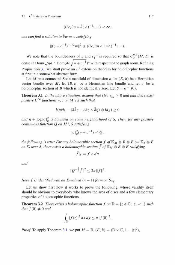
3.1 L2 Extension Theorems 117
((ic2∂η ∧ ∂ηΛ)−1v, v) <∞,
one can find a solution to ∂w = v satisfying
‖(η + c−11 )−1/2w‖2 ≤ ((ic2∂η ∧ ∂ηΛ)−1v, v).
We note that the boundedness of η and c−11 is required so that Cn,q
0 (M,E) is
dense in Dom(√η∂)∩Dom(∂◦
√η + c−1
1 )∗ with respect to the graph norm. Refining
Proposition 3.1 we shall prove an L2 extension theorem for holomorphic functionsat first in a somewhat abstract form.
Let M be a connected Stein manifold of dimension n, let (E, h) be a Hermitianvector bundle over M , let (B, b) be a Hermitian line bundle and let σ be aholomorphic section of B which is not identically zero. Let S = σ−1(0).
Theorem 3.1 In the above situation, assume that iΘh|Sreg ≥ 0 and that there existpositive C∞ functions η, c on M \ S such that
i(ηΘh − (∂∂η + c∂η ∧ ∂η)⊗ IdE) ≥ 0
and η + log |σ |2b is bounded on some neighborhood of S. Then, for any positivecontinuous function Q on M \ S satisfying
|σ |2b(η + c−1) ≤ Q,
the following is true: For any holomorphic section f of KM ⊗ B ⊗ E (= KS ⊗ E
on S) over S, there exists a holomorphic section f of KM ⊗ B ⊗ E satisfying
f |S = f ∧ dσ
and
‖Q− 12 f ‖2 ≤ 2π‖f ‖2.
Here f is identified with an E-valued (n− 1) form on Sreg.
Let us show first how it works to prove the following, whose validity itselfshould be obvious to everybody who knows the area of discs and a few elementaryproperties of holomorphic functions.
Theorem 3.2 There exists a holomorphic function f on D = {z ∈ C; |z| < 1} suchthat f (0) �= 0 and ∫
D
|f (z)|2 dx dy ≤ π |f (0)|2.
Proof To apply Theorem 3.1, we put M = D, (E, h) = (D× C, 1− |z|2),
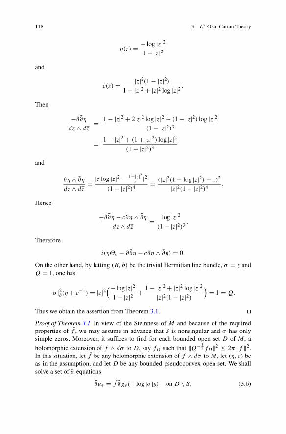
118 3 L2 Oka–Cartan Theory
η(z) = − log |z|21− |z|2
and
c(z) = |z|2(1− |z|2)1− |z|2 + |z|2 log |z|2 .
Then
−∂∂ηdz ∧ dz =
1− |z|2 + 2|z|2 log |z|2 + (1− |z|2) log |z|2(1− |z|2)3
= 1− |z|2 + (1+ |z|2) log |z|2(1− |z|2)3
and
∂η ∧ ∂ηdz ∧ dz =
|z log |z|2 − 1−|z|2z|2
(1− |z|2)4 = (|z|2(1− log |z|2)− 1)2
|z|2(1− |z|2)4 .
Hence
−∂∂η − c∂η ∧ ∂ηdz ∧ dz = log |z|2
(1− |z|2)3 .
Therefore
i(ηΘh − ∂∂η − c∂η ∧ ∂η) = 0.
On the other hand, by letting (B, b) be the trivial Hermitian line bundle, σ = z andQ = 1, one has
|σ |2b(η + c−1) = |z|2(− log |z|2
1− |z|2 +1− |z|2 + |z|2 log |z|2|z|2(1− |z|2)
)= 1 = Q.
Thus we obtain the assertion from Theorem 3.1. ��Proof of Theorem 3.1 In view of the Steinness of M and because of the requiredproperties of f , we may assume in advance that S is nonsingular and σ has onlysimple zeros. Moreover, it suffices to find for each bounded open set D of M , a
holomorphic extension of f ∧ dσ to D, say fD such that ‖Q− 12 fD‖2 ≤ 2π‖f ‖2.
In this situation, let f be any holomorphic extension of f ∧ dσ to M , let (η, c) beas in the assumption, and let D be any bounded pseudoconvex open set. We shallsolve a set of ∂-equations
∂uε = f ∂χε(− log |σ |b) on D \ S, (3.6)

3.1 L2 Extension Theorems 119
where 0 < ε < 1e
and
χε(t) =⎧⎨⎩
0 if t < − log εlog t − log(− log ε) if − log ε ≤ t ≤ −e log ε1 if t > −e log ε.
with side conditions of uε such that uε are extendable to D continuously in such away that uε |S∩D = 0 and
lim infε→0
‖Q− 12 uε‖2 ≤ 2π‖f ‖2. (3.7)
Then a subsequence of f χε(− log |σb|) − uε will converge to a desired extension.To find uε , we fix a Kähler metric on D \ S and apply a general formula (3.5) foru ∈ Cn,q
0 (D \ S,E) by modifying the given η and c to ηε and cε as follows.We first put
ηε(z)=
⎧⎪⎨⎪⎩η(z) (ε<|σ(z)|b)min
{η(z),− log |σ(z)|2
b+ log |σ(z)|b log
( log |σ(z)|blog ε
)}(εe ≤ |σ(z)|b ≤ ε)
−e log ε (|σ(z)|b<εe)
Then, by using iΘh|S ≥ 0, the boundedness of η + log |σ |2b near S and theSteinness of M to obtain positive C∞ functions ηε , cε and dε which approximateηε , c and 0 on M \ S in such a way that they satisfy
i(ηεΘh⊗b|σ |−2
b− ∂∂ηε − cε∂ηε ∧ ∂ηε
)≥ 0,
i(ηεΘh⊗b|σ |−2
b− ∂∂ηε − cε∂ηε ∧ ∂ηε
)
≥ i((1− dε)∂ log |σ |b ∧ ∂ log |σ |b/(− log |σ |b)) (εe < |σ(z)| < ε),
and
(1− dε)(ηε + c−1ε )|σ |2b ≤ Q. (3.8)
Thus we obtain uε such that uε |D∩S = 0 and
(1− dε)−1‖(ηε + c−1
ε )−12 uε‖2
h⊗b|σ |−2b
≤ 2π‖f ‖2. (3.9)
Combining (3.8) and (3.9) we obtain the required estimate
‖Q− 12 uε‖2h⊗b ≤ 2π‖f ‖2. ��
Theorem 3.1 implies the following similarly to Theorem 3.2.
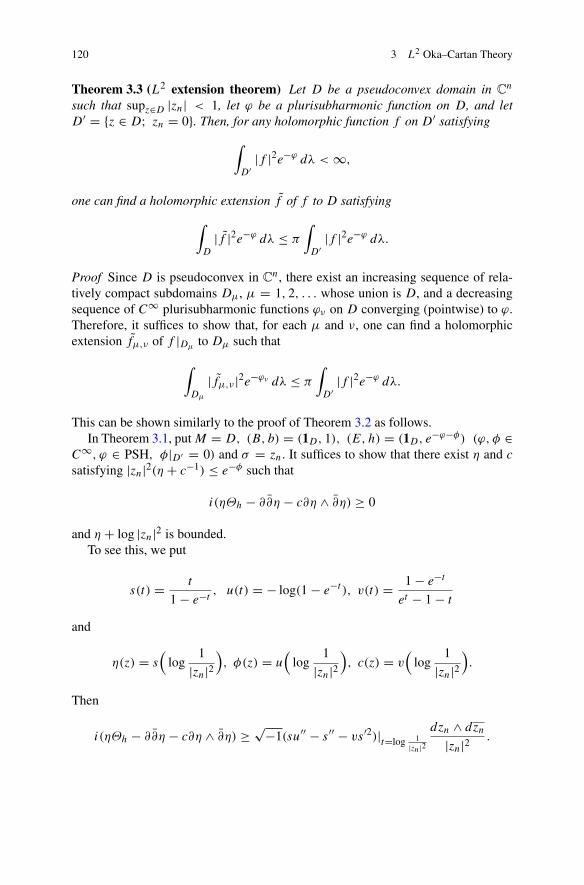
120 3 L2 Oka–Cartan Theory
Theorem 3.3 (L2 extension theorem) Let D be a pseudoconvex domain in Cn
such that supz∈D |zn| < 1, let ϕ be a plurisubharmonic function on D, and letD′ = {z ∈ D; zn = 0}. Then, for any holomorphic function f on D′ satisfying
∫D′|f |2e−ϕ dλ <∞,
one can find a holomorphic extension f of f to D satisfying
∫D
|f |2e−ϕ dλ ≤ π
∫D′|f |2e−ϕ dλ.
Proof Since D is pseudoconvex in Cn, there exist an increasing sequence of rela-
tively compact subdomains Dμ, μ = 1, 2, . . . whose union is D, and a decreasingsequence of C∞ plurisubharmonic functions ϕν on D converging (pointwise) to ϕ.Therefore, it suffices to show that, for each μ and ν, one can find a holomorphicextension fμ,ν of f |Dμ to Dμ such that
∫Dμ
|fμ,ν |2e−ϕν dλ ≤ π
∫D′|f |2e−ϕ dλ.
This can be shown similarly to the proof of Theorem 3.2 as follows.In Theorem 3.1, put M = D, (B, b) = (1D, 1), (E, h) = (1D, e−ϕ−φ) (ϕ, φ ∈
C∞, ϕ ∈ PSH, φ|D′ = 0) and σ = zn. It suffices to show that there exist η and csatisfying |zn|2(η + c−1) ≤ e−φ such that
i(ηΘh − ∂∂η − c∂η ∧ ∂η) ≥ 0
and η + log |zn|2 is bounded.To see this, we put
s(t) = t
1− e−t, u(t) = − log(1− e−t ), v(t) = 1− e−t
et − 1− t
and
η(z) = s(
log1
|zn|2), φ(z) = u
(log
1
|zn|2), c(z) = v
(log
1
|zn|2).
Then
i(ηΘh − ∂∂η − c∂η ∧ ∂η) ≥ √−1(su′′ − s′′ − vs′2)|t=log 1
|zn|2dzn ∧ dzn|zn|2 .

3.1 L2 Extension Theorems 121
Since
s(t) = eu(t)∫ t
0e−u(x)dx
s′
s= (log s)′ = u′ + 1
s,
Hence s′ − su′ = 1,
s′2
su′′ − s′′= − s
′
u′= et − 1− t
1− e−t= 1
v
so that
√−1(ηΘh − ∂∂η − c∂η ∧ ∂η) ≥ 0
is obtained. ��Remark 3.1 Theorem 3.3 was first proved by Błocki [Bł-2] to settle a questionposed by Suita [Su-1]. Related materials will be discussed in more detail in thenext chapter. (See also 3.4 in this chapter.)
3.1.2 L2 Extension Theorems on Complex Manifolds
We shall formulate L2 extension theorems in more general settings in such a waythat they include some of the interpolation theorems in classical complex analysisin one variable. The proofs are essentially the same as in Theorem 3.3.
Definition 3.1 A complex manifold M with a closed subset A is said to be a quasi-Stein manifold if A satisfies the following two conditions:
(1) M \ A is a Stein manifold.(2) Each point x ∈ A has a fundamental neighborhood system Ux in M such that,
for every U ∈ Ux , the natural restriction map
O(U) −→ {f ∈ L0,0(2),loc(U); f |U\A is holomorphic}
is surjective.
Example 3.1 A complex manifold M with a nowhere-dense closed analytic subsetA is quasi-Stein if M \A is a Stein manifold. In particular, a nonsingular projectivealgebraic variety with a hyperplane section is quasi-Stein.
The following is obvious.
122 3 L2 Oka–Cartan Theory
Proposition 3.2 Let (M,A) be a connected quasi-Stein manifold of dimension ≥1. Then A is nowhere dense in M .
Theorem 3.4 Let (M,A) be a quasi-Stein manifold of dimension n, let w be aholomorphic function on M , let H = w−1(0), and let H0 = w−1(0) \ dw−1(0).Suppose that H0\A is dense in H . Let φ and ψ be plurisubharmonic functions onM such that sup (ψ + 2 log |w|) ≤ 0. Then, for any holomorphic (n − 1)-form f
on H0 satisfying | ∫H0e−φf ∧ f | <∞, there exists a holomorphic n-form F on M
such that F = dw ∧ f holds at any point of H0 and
∣∣∣∫M
e−φ+ψF ∧ F∣∣∣ ≤ 2π
∣∣∣∫H0
e−φf ∧ f∣∣∣. (3.10)
Proof By the condition (2) on A, it suffices to show the assertion for the manifoldM \ A. Since M \ A is Stein, it is an increasing union of strongly pseudoconvexdomains. Therefore, we may assume that φ and ψ are smooth and it suffices to find,for each relatively compact Stein domain Ω in M \A, a holomorphic n-form FΩ onΩ such that FΩ = dw ∧ f holds at any point of H0 ∩Ω and
∣∣∣∫Ω
e−φ+ψFΩ ∧ FΩ∣∣∣ ≤ 2π
∣∣∣∫H0
e−φf ∧ f∣∣∣. (3.11)
To prove this, one has only to repeat the argument of the proof of Theorem 3.2.Namely, by lettingψ+log |w|2 play the role of log |z|2 in defining η and by applyingthe formula (3.5) for h = e−φ−log |w|2 , we are done. ��Remark 3.2 Theorem 3.3 was first established for the case ψ ≡ 0 in [Oh-T-1],where the estimate for F is not sharp. The motivation of introducing ψ in [Oh-17]was to improve the known estimate for the Bergman kernel from below. (For thedetail, see the next chapter.) In [Oh-17], φ−ψ was assumed to be plurisubharmonic.The present form with an optimal estimate was first established in [G-Z-1].
Now let us proceed to a more general case. Given a positive measure dμM on M ,we shall denote by A2(M,E, h, dμM) the space of L2 holomorphic sections of Eover M with respect to h and dμM . Let S be a closed complex submanifold of Mand let dμS be a positive measure on S. A2(S,E, h, dμS) will stand for the spaceof L2 holomorphic sections of E over S with respect to h and dμS .
Definition 3.2 (S, dμS) is said to be a set of interpolation for A2(M,E, h, dμM)
if there exists a bounded linear operator I from A2(S,E, h, dμS) to A2(M,E, h,
dμM) such that I (f )|S = f holds for any f .
Let dVM be any continuous volume form on M . Then we consider a class ofcontinuous functions Ψ from M to [−∞, 0) such that:
(1) Ψ−1(−∞) ⊃ S
and
3.1 L2 Extension Theorems 123
(2) if S is k-dimensional around a point x, there exists a local coordinate z =(z1, z2, . . . , zn) on a neighborhood U of x such that zk+1 = · · · = zn = 0on S ∩ U and
supU\S|Ψ (z)− (n− k) log
n∑k+1
|zj |2| <∞.
The set of such functions Ψ will be denoted by �(S). Clearly, the condition (2) doesnot depend on the choices of local coordinates. For each Ψ ∈ �(S) we define apositive measure dVM [Ψ ] on S as the minimum element of the partially ordered setof positive measures dμ satisfying
∫Sk
f dμ ≥ lim supt→∞
2(n− k)
σ2n−2k−1
∫M
f e−Ψ χR(Ψ, t) dVM
for any nonnegative continuous function f with supp f � M , where Sk denotes thek-dimensional component of S, σm denotes the volume of the unit sphere in R
m+1,and χR(Ψ, t) the characteristic function of the set
R(Ψ, t) = {x ∈ M; −t − 1 < Ψ (x) < −t}.
Note that the coefficient 2(n − k)/σ2n−2k−1 is chosen in such a way thatdλz[log |zn|2] = dλz′ for z = (z′, zn).
Theorem 3.5 (L2 extension theorem on manifolds) LetM be a complex manifoldwith a continuous volume form dVM , let (E, h) be a Nakano semipositive vectorbundle over M , let S be a closed complex submanifold of M , let Ψ ∈ �(S) ∩C∞(M \ S) and let KM be the canonical bundle of M . Then (S, dVM [Ψ ]) is aset of interpolation for A2(M,E ⊗ KM, h ⊗ (dVM)
−1, dVM) if the following aresatisfied:
(1) There exists a closed subset A such that S∩A is nowhere dense in S and (M,A)
is quasi-Stein.(2) There exists a positive number δ such that he−(1+δ)Ψ is a Nakano semipositive
singular fiber metric of E.
If, moreover, Ψ is plurisubharmonic on M , the interpolation operator fromA2(S,E⊗KM, h⊗(dVM)−1, dVM [Ψ ]) toA2(M,E⊗KM, h⊗(dVM)−1, dVM)
can be chosen so that its norm does not exceed√π .
Sketch of proof. Similarly to Theorem 3.4 it suffices to prove that, for everyrelatively compact Stein domain Ω in M \A, there exists a bounded linear map IΩ :A2(S,E⊗KM, h⊗ (dVM)−1, dVM [Ψ ])→ A2(Ω,E⊗KM, h⊗ (dVM)−1, dVM)
whose norm is bounded by a constant independent of Ω such that IΩ(f )|S∩Ω =f |S∩Ω holds for all f ∈ A2(S,E ⊗ KM, h ⊗ (dVM)
−1, dVM [Ψ ]). When Ψ isplurisubharmonic, the main difference from the situation of Theorem 3.4 is that

124 3 L2 Oka–Cartan Theory
S ∩ Ω is not necessarily defined as the zero set of a single holomorphic function.However, the assumption on Φ was made in such a way that, as was indicated aboveby the equation dλz[log |zn|2] = dλz′ , Ψ plays the same role as log |w|2 in the proofof Theorem 3.4. For the proof of the first part, see [Oh-19]. ��Remark 3.3 Theorem 3.5 with a weaker bound 24√π of the interpolation operatorfor the last statement was obtained in [Oh-19]. A proof for the bound
√π was found
in [G-Z-1].
Compared to Theorem 3.4, the advantage of Theorem 3.5 is that the condition onthe set S is stated in terms of a measure on S and a function with value −∞ alongS, since it is often hard to find a generator of the ideal of holomorphic functionsvanishing along S. The prototype of Theorem 3.5 is a theorem on interpolation andsampling in one variable due to K. Seip, which we shall recall below. For the proofsthe reader is referred to [Sp-1, Sp-2] and [S-W].
Definition 3.3 A subset Γ ⊂ C is said to be uniformly discrete if
inf {|z− w|; z,w ∈ Γ, z �= w} > 0.
The upper uniform density of a uniformly discrete set Γ is defined to be
lim supr→∞
supw
�{z ∈ Γ ; |z− w| < r}πr2 ,
which will be denoted by D+(Γ ).
For simplicity we put
A2α = A2(C,C× C, e−α|z|2 , dλz).
Theorem 3.6 Let Γ be a uniformly discrete subset of C and let δΓ be the Diracmass supported on Γ . Then, (Γ, δΓ ) is a set of interpolation for A2
α if and only ifα > πD+(Γ ).
For the unit disc D we put
A2α,D = A2(D,D× C, (1− |z|2)α, dλz).
Definition 3.4 A subset Γ ⊂ D is said to be uniformly discrete if
inf{∣∣∣ z− w
1− zw
∣∣∣; z,w ∈ Γ, z �= w}> 0.
Letting ρ(z,w) = | z−w1−zw | we put
D+D(Γ ) = lim sup
r→1supz
∑ξ∈Γ, 1
2<ρ(z,ξ)<rlog ρ(z, ξ)
log (1− r).

3.1 L2 Extension Theorems 125
Theorem 3.7 Let Γ be a uniformly discrete subset of D. Then (Γ, (1− |z|2)δΓ ) isa set of interpolation for A2
α,D if and only if α > 2D+D(Γ ).
Theorems 3.6 and 3.7 are related to Theorem 3.5 through an interpretation of thedensity concepts in the following manner.
For any discrete set Γ ⊂ C we set
C+(Γ ) = inf {α; there exists a Ψ ∈ �(Γ ) such that Ψ + α|z|2is subharmonic on C}.
For a discrete set Γ ⊂ D we put
C+D(Γ ) = inf {α; there exists a Ψ ∈ �(Γ ) such that Ψ − α log (1− |z|2)
is subharmonic on C}.
Theorem 3.8 For any uniformly discrete subset Γ ⊂ C (resp. Γ ⊂ D) one hasπD+(Γ ) = C+(Γ ) (resp. 2D+
D(Γ ) = C+
D(Γ )).
For the proof, see [Oh-19].
3.1.3 Application to Embeddings
Although it might look unlikely from the above exposition, L2 extension theoremshave applications to algebraic geometry. They are used effectively in the inductionon the dimension. Uniformity of the estimate in the weight factor ϕ is important forthat purpose. A typical example of such application is to a question of T. Fujita:
Fujita’s Conjecture (cf. [F-2]) Let M be a nonsingular projective variety over Cof dimension n, and let L→ M be an ample line bundle. Then:
(1) KM ⊗ L⊗(n+1) is generated by global sections and(2) KM ⊗ L⊗(n+2) is very ample.
It is obvious that Fujita’s conjecture is true if M = CPn. A theorem of Lefschetz
implies its validity for the case of Abelian varieties. There have been a number ofresults on part (1) of Fujita’s conjecture, including its full verification for n ≤ 5 (cf.[Rd, Ko, E-L, F-3, Km-4, Y-Z’15]) and its partial verification for general n whichrequires m to be greater than a constant of order n2 (cf. [A-S, H-1, H-2, Hei]). Asfor the connections of Fujita’s conjecture to other questions of algebraic geometry,see [M-2] and [Km-1, Km-2, Km-4] as well as [F-2]. In [A-S], Theorem 3.3 (witha weaker estimate) is used to show a semicontinuity property for multiplier idealsheaves which naturally yields the following effective partial solution to Fujita’sconjecture.

126 3 L2 Oka–Cartan Theory
Theorem 3.9 (cf. Angehrn and Siu [A-S]) Let M and L be as above and let κ bea positive number. Suppose that, for any irreducible subvariety W of dimension 1 ≤d ≤ n inM , the degreeLd ·W ofL|W satisfies (Ld ·W)
1d ≥ 1
2n(n+2r−1)+κ . Thenthe global sections of OM(KM ⊗L) separate any set of r distinct points P1, . . . , Prof M .
Corollary 3.1 KM ⊗ Lm is generated by global sections if m ≥ 12 (n
2 + n+ 2).
Combining Corollary 3.1 with the following lemma, it is known that KM ⊗ L⊗(KM ⊗ Lm)n+1 is very ample for m ≥ 1
2 (n2 + n+ 2).
Lemma 3.1 Let L be a positive line bundle over a compact complex manifold M ofdimension n such that OM(L) is generated by global sections. Then, KM⊗Ln+1⊗Ais very ample for any positive line bundle A.
The method of Angehrn and Siu was applied by Takayama [Ty-1] to establisha projective embedding theorem for pseudoconvex manifolds with positive linebundles, which amounts to a partial solution to the following generalization ofFujita’s conjecture:
Let M be a pseudoconvex manifold of dimension n and let L be a positive linebundle over M .
Generalized Fujita’s Conjecture
(1) KM ⊗ L⊗(n+1) is generated by global sections
and
(2) KM ⊗ L⊗(n+2) is very ample.
Theorem 3.10 (cf. [Ty-1]) Let M be an n-dimensional pseudoconvex manifoldwith a positive line bundle L. Then KM ⊗ Lm is generated by global sections ifm > 1
2n(n+ 1), and (KM ⊗ Lm)� is very ample if m > 12n(n+ 1) and � > n+ 1.
The proofs of Theorems 3.9 and 3.10 follow from Nadel’s vanishing theoremonce one has appropriate singular fiber metrics. Such singular fiber metrics areconstructed from the sections of sufficiently high tensor powers of the line bundleL. To obtain a “sufficiently singular” fiber metric by this method, one needs aninduction, and at this step the L2 extension theorem plays a crucial role.
Let us have a glance at this argument by tracing a lemma on the semicontinuityof multiplier ideal sheaves in Siu’s exposition [Siu-6]. In the following, “s is amultivalued section of the fractional bundle L
ab ” means that sb is a section of the
bundle La .
Lemma 3.2 Let M be a compact complex manifold of complex dimension n andlet L be a positive line bundle over M . Let P0 be a point of M and U ′ be alocal holomorphic curve in M passing through P0 with P0 as the only (possible)singularity. Let U be the open unit disc in C and σ : U → U ′ be the normalizationof U ′ so that σ(0) = P0. Let β be a positive rational number. Let s1, . . . , sk be mul-tivalued holomorphic sections of pr∗1 (Lβ) over M × U (pr1 denotes the projection
3.1 L2 Extension Theorems 127
to the first factor.). Suppose that for almost all u ∈ U \ {0} (in the sense that thestatement is true up to a subset of measure zero) the point (σ (u), u) belongs to thezero-set of the multiplier ideal sheaf of the singular metric (
∑kν=1 |sν |2)−1|M×{u}
of Lβ = pr∗1 (Lβ)|M×{u} (i.e. the function (∑k
ν=1 |sν |2)−1(·, u) is not locallyintegrable at σ(u)). Then (P0, 0) belongs to the zero-set of the multiplier idealsheaf of the singular metric (
∑kν=1 |sν |2)−1|M×{0} of Lβ = pr∗1 (Lβ)|M×{0} (i.e.
the function (∑k
ν=1 |sν |2)−1(·, 0) is not locally integrable at P0).
Proof Assume the contrary. Then for some open neighborhood V of P0 in M thefunction (
∑kν=1 |sν |2)−1(·, 0) is integrable on V . We can assume without loss of
generality that pr∗1L|V×U is holomorphically trivial and V is biholomorphic to abounded pseudoconvex domain in C
n. We apply Theorem 3.3 to the domain D =V × U and the hyperplane H = C
n × {0} for zn = 0. For the plurisubharmonicfunction we use ϕ = log (
∑kν=1 |sν |2) and for the function to be extended we use
f ≡ 1. Let F be the holomorphic function on V × U such that
∫V×U|F |2
( k∑ν=1
|sν |2)−1
<∞
and F(·, 0) = f on V . There exist an open neighborhood V ′ of P0 in V andan open neighborhood W of 0 in U such that |F | is bounded from below onV ′ × W by some positive number. There is a set E of measure zero in W suchthat
∫V ′×{u} (
∑kν=1 |sν |2)−1 is finite for u ∈ W \ E, contradicting the assumption
that (∑k
ν=1 |sν |2)−1(·, u) is not locally integrable at σ(u) for almost all u ∈ U \ {0}.��
3.1.4 Application to Analytic Invariants
Given a compact complex manifold M , dimH 0,0(M,KmM) (m ∈ N) is called the
(m-th) plurigenus of M and denoted by Pm = Pm(M). S. Iitaka asked whetheror not Pm is invariant under deformation (cf. [Nk]). Namely, let π : M → D bea smooth family of compact complex manifolds and let Mt = π−1(t). Then is ittrue that Pm(Mt) = Pm(M0) for all t? Nakamura [Nk’72] found that there exists acompact 3-fold M0 with trivial canonical bundle which admits a small deformationM ′ such that H 3,0(M ′) = 0, so that at least one plurigenus of M0, namely P1, isnot invariant under deformation. Since Nakamura’s example M0 is non-Kähler, theinvariance of Pm for compact Kähler manifolds was left open. Although the fullconjecture is still open, it was verified for algebraic manifolds in [Siu-7, Siu-9] (seealso [T’02]). Siu’s proof combines the L2 extension theorem and Skoda’s divisiontheorem (see the next section for Skoda’s division theorem). An alternate proofusing only the L2 extension was given by Paun [P]. Moreover, Paun’s method wasgeneralized by Claudon [Cl’07] to prove an extension theorem which is a relativeversion of the following.
128 3 L2 Oka–Cartan Theory
Theorem 3.11 (cf. [Ty’06]) Let X be a projective algebraic manifold, let S ⊂ X
be a nonsingular irreducible hypersurface and let L → X be a holomorphic linebundle equipped with a singular fiber metric h such that
(i) Θh ≥ εω (with ε > 0 for some C∞ Hermitian metric ω on X)
and
(ii) the restriction hS of the metric h to S is well defined and IhS = OS .
Then, for any integer m ≥ 1 the natural restriction map
H 0(X,O(KX ⊗ [S] ⊗ L)⊗m) −→ H 0(S,O(KS ⊗ L)⊗m)
is surjective.
The circumstance of Claudon’s theorem is as follows. Let π :M → D be a properholomorphic submersion and let L →M be a positive line bundle with a singularfiber metric h such that
(i) Θh ≥ 0 ((L , h) is pseudo-effective)(ii) h0 := h|M0 is well-defined as a singular fiber metric
and(iii) Ih0 = OM0 .
Theorem 3.12 In the above situation, the restriction map
H 0(M ,O(KM ⊗L )⊗m) −→ H 0(M0,O(KM0 ⊗L )⊗m)
is surjective.
Obviously the invariance of plurigenera is an immediate corollary of Theorem 3.12.The main tool of the proof is the following variant of Theorem 3.3.
Theorem 3.13 (cf. [Siu’02]) In the situation of Theorem 3.12, there exists a(universal) constant C0 such that for every section σ0 ∈ H 0(M0,O(KM0 ⊗ L ))
satisfying∫M0|σ ∧ σ |h < ∞, there exists σ ∈ H 0(M ,O(KM ⊗ L )) with
σ |M0 = σ ∧ dt and∫M |σ ∧ σ |h ≤ C0
∫M0|σ ∧ σ |h.
3.2 L2 Division Theorems
Given holomorphic functions g1, . . . , gm on a pseudoconvex domain D over Cn,Oka [O-2] proved that, for any holomorphic function h on D which is locally in theideal generated by gj (1 ≤ j ≤ m), one can find holomorphic functions fj (1 ≤ j ≤m) on D such that h =∑m
j=1 fjgj holds on D. In Cartan’s terminology, this is dueto the coherence of the kernel of the sheaf homomorphism

3.2 L2 Division Theorems 129
g : Om −→ O, g(u1, . . . , um) =m∑j=1
ujgj
and the vanishing of the first cohomology of D with coefficients in the coherentanalytic sheaves (cf. [G-R]). The L2 method of Hörmander [Hö-1, Hö-2] wasapplied by Skoda [Sk-2] to obtain an effective quantitative refinement of Oka’stheorem. After reviewing Skoda’s theory in its generalized form (cf. [Sk-4]), weshall show that an L2 extension theorem on complex manifolds can be appliedto prove an L2 division theorem. This approach has an advantage that it yields adivision theorem with an optimal L2 estimate in some cases.
3.2.1 A Gauss–Codazzi-Type Formula
Let M be a complex manifold and let (Ej , hj ) (j = 1, 2) be two Hermitianholomorphic vector bundles. By a morphism between (E1, h1) and (E2, h2), weshall mean a holomorphic bundle morphism γ : E1 → E2 such that γ |(Ker γ )⊥fiberwise preserves the length of vectors. Here (Ker γ )⊥ denotes the orthogonalcomplement of Ker γ . Let
0 −→ S −→ E −→ Q −→ 0 (3.12)
be a short exact sequence of holomorphic vector bundles over M and let h be a fibermetric of E. Then one has fiber metrics of S and Q, say hS and hQ respectively,for which the arrows in (3.12) become morphisms of Hermitian holomorphic vectorbundles. There is a relation between the curvature forms of h, hS and hQ which issimilar to the classical Gauss–Codazzi formula. It was found by Griffiths [Gri-1,Gri-3]. The presentation below follows [Gri-1, Gri-3] and [Sk-4].
Let DE be the Chern connection of (E, h) (cf. Chap. 1). Then DE is decomposedaccording to the orthogonal decomposition E = S ⊕Q:
DE =(DS −B∗B DQ
), (3.13)
where DS and DQ denote respectively the Chern connections of (S, hS) and(Q, hQ), B = ∑
Bα dzα ∈ C1,0(M,Hom(S,Q)), and B∗ = ∑
B∗α dzα ∈C0,1(M,Hom(Q, S)), where B∗α denotes the adjoint of Bα . With respect to a localframe (s1, . . . , sm) of E extending a local frame (s1, . . . , s�) of S,
Bα = (Bμαν) =
( �∑σ=1
hμσ∂hνσ
∂zα
).

130 3 L2 Oka–Cartan Theory
In other words, if s and t are respectively smooth sections of S and Q over anopen set of M ,
DE(s + t) = DSs − B∗t + Bs +DQt.
B is called the second fundamental form of S ⊕ Q. Note that the secondfundamental forms of S⊕Q and (S⊗L)⊕ (Q⊗L) are equal for any holomorphicHermitian line bundle L.
Example 3.2 Let M = C, let E = C×C2, let Q = C×C, let g : E→ Q be given
by (z, (ζ, ξ))→ (z, (zζ, ξ)), let h = (δμν), and let S = Ker g. Then
S ⊕Q = C · (1,−z)⊕ C · (z, 1),
|1|2hS = 1+ |z|2,|1|2
hQ= (|z|2 + 1)−1,
B(1,−z) = (0,−dz)
and
B∗(1) = dz.
Recall that the curvature form Θh is defined as a Hom(E,E)-valued (1,1)-formon M satisfying
D2Es = Θhs (3.14)
for any local C∞ section s of E. Therefore, from (3.13) one immediately obtains
Θh =(D2S − B∗ ∧ B −D(B∗)D(B) D2
Q − B ∧ B∗)
(3.15)
where D(B) denotes the derivative of B with respect to the connection ofHom(S,Q) associated to DS and DQ, namely
DQ(rs) = (Dr)s + r(DSs)
for local sections r of Hom(S,Q) and s of S. In particular, one has ∂B∗ = 0. From(3.15) we obtain the vector bundle version of the Gauss–Codazzi formula:
{ΘhS = Θh|S + B∗ ∧ B,ΘhQ = Θh|Q + B ∧ B∗. (3.16)

3.2 L2 Division Theorems 131
Here the restrictions of Θh are with respect to the orthogonal decomposition E =S⊕Q. In terms of the local coordinates such that h = (hμν) andB = (
∑α B
κανdz
α),
{(ΘhS )
μ
ναβ= (Θh)
μ
ναβ−∑κ,σ,ρ B
κανh
μσBρβσ hκρ,
(ΘhQ)κ
ραβ= (Θh)
κ
ραβ+∑μ,ν,σ B
κανh
νμBσβμhρσ .
(3.17)
Note that the cohomology class in H 1(M,Hom(Q, S)) represented by B∗vanishes if and only if (3.12) splits as a short exact sequence of holomorphic vectorbundles. To see this, let g be the given morphism fromE toQ and let j be the sectionof Hom(Q,E)which satisfies g◦j = IdQ and embedsQ intoE isometrically. From(3.13), for any C∞ section t of Q one has
{∂(j t) = −B∗t + ∂ t,
∂(j t) = (∂j)t + j ∂t.(3.18)
Hence
∂j = −B∗.
If there exists A ∈ C∞(M,Hom(Q, S)) satisfying
∂A = −B∗,
then j −A is a holomorphic bundle morphism from Q to E such that g ◦ (j −A) =idQ.
Now, given a holomorphic section f of Q, one has ∂(jf ) = −B∗f , so that∂(B∗f ) = 0. If there exists a solution u ∈ C∞(M, S) to the equation
∂u = −B∗f, (3.19)
f − u will then be holomorphic and satisfy
g(f − u) = f. (3.20)
Therefore, the problem of lifting holomorphic sections of Q to those of E is reducedto solving the ∂ equations of the form (3.19) with values in S. In the next subsection,we shall review how Skoda solved a division problem under this formulation.
3.2.2 Skoda’s Division Theorem
As well as in the case of extension theorems, it is most appropriate to state a generalL2 division theorem for the bundle-valued (n, 0)-forms on n-dimensional complete
132 3 L2 Oka–Cartan Theory
Kähler manifolds. Let (M,ω) be a complete Kähler manifold of dimension n andlet 0 → S → E → Q → 0, g : E → Q, h and B∗ be as above. From nowon, the ranks of S,E and Q will be denoted by s, p and q, respectively. For thedivision theorem, Nakano’s identity is combined with the following lemma whichSkoda called “LEMME FONDAMENTAL”.
Lemma 3.3 Let r = min {n, s} = min {n, p − q}. For any form v ∈ Cn,1(M, S)
and β ∈ C1,0(M,Hom(S,Q)) one has:
r〈i Trββ∗ ⊗ IdSΛv, v〉 ≥ |β�v|2 (3.21)
at every point of M , where Trββ∗ denotes the trace of β ∧ β∗ ∈ C1,1(M,Hom(Q,Q)) and β� the adjoint of exterior multiplication by β∗.
Proof By using the local orthonormal frames, (3.21) follows from the Cauchy–Schwarz inequality
∣∣∣s∑
k=1
ak
∣∣∣2 ≤ s
s∑k=1
|ak|2
if r = s. If r = n, (3.21) is reduced to the inequality
n
s∑k,�=1
∣∣∣∑λ
βkλv�λ
∣∣∣2 ≥∣∣∣∑k,λ
βkλvkλ
∣∣∣2.
For the detail, see [Sk-4, pp. 591–594]. ��In the sense of Nakano positivity similar to the case of curvature form of vector
bundles, the lemma says that irTrββ∗ ⊗ IdS + iββ∗ ≥ 0. Hence, in view of (3.16)and
TrΘhQ = ΘdethQ
one has the following L2 estimate.
Proposition 3.3 Assume that (E, h) is Nakano semipositive and let (L, b) be aHermitian holomorphic line bundle over M whose curvature form Θb satisfies
iΘb ≥ i(r + ε)ΘdethQ (3.22)
for some ε > 0. Then
‖∂u‖2 + ‖∂∗u‖2 ≥ ε
r‖B�u‖2 (3.23)
holds for any u ∈ Cn,10 (M, S ⊗ L).
3.2 L2 Division Theorems 133
Example 3.3 In the case of Example 3.2, (3.22) holds for (L, b) = (C×C, (|z|2 +1)−1−ε).
Hence, solving the equation (3.19) with an L2 estimate based on (3.23),Lemma 2.1 and Theorem 2.3, one has:
Theorem 3.14 Let the situation be as in Proposition 3.2. Then, for any Q ⊗ L-valued holomorphic n-form f on M which is square integrable with respect to ω
and hQ⊗b, there exists an E⊗L-valued holomorphic n-form e such that f = g · eand
‖e‖2 ≤(
1+ r
ε
)‖f ‖2. (3.24)
Corollary 3.2 Suppose that (E ⊗ detE, h ⊗ det h) is Nakano semipositive and aHermitian holomorphic line bundle (L, b) over M satisfies
iΘb − iΘdeth − i(r + ε)ΘdethQ ≥ 0
for some ε > 0. Then the map
Hn,0(2) (M,E ⊗ L) −→ H
n,0(2) (M,Q⊗ L)
induced from g is surjective.
Proof It suffices to apply Theorem 3.11 for the morphism E⊗ detE→ Q⊗ detEand the line bundle (detE)∗ ⊗ L. ��Remark 3.4 It was recently shown by Liu, Sun and Yang [L-S-Y] that ample vectorbundles have fiber metrics such that Θh⊗deth is Nakano positive. satisfying thecondition of h in Corollary 3.2. See also [Dm-S].
Applying Corollary 3.2 when M is a bounded pseudoconvex domain in Cn and
h = (δμν), one has the followng.
Corollary 3.3 LetD be a bounded pseudoconvex domain in Cn, let φ be a plurisub-
harmonic function on D and let g = (g1, . . . , gp) be a vector of holomorphicfunctions on D. If f is a holomorphic function on D such that
∫D
|f |2|g|−2k−2−εe−φ dλ <∞
holds for k = min {n, p − 1} and some ε > 0, there exists a vector of holomorphicfunctions a = (a1, . . . , ap) satisfying
f =p∑j=1
ajgj
134 3 L2 Oka–Cartan Theory
and∫D
|a|2|g|−2k−εe−φ dλ <∞.
An advantage of Corollary 3.3 is that it has the following division theorem as animmediate consequence. This special case is useful for the construction of integralkernels (cf. [He]).
Theorem 3.15 Let D be a bounded domain in Cn which admits a complete Kähler
metric and let z = (z1, . . . , zn) be the coordinate of Cn. Then, for any positivenumber ε, there exists a constant Cε such that, for any holomorphic function f onD satisfying
∫D
|f (z)|2|z|−2n−ε dλ <∞,
one can find a system of holomorphic functions a = (a1, . . . , an) satisfying
f (z) =n∑
j=1
zjaj (z)
and∫D
|a(z)|2|z|−2n+2−ε dλ ≤ Cε
∫D
|f (z)|2|z|−2n−ε dλ.
Corollary 3.4 (cf. [D-P]) Let D be a domain in Cn which admits a complete
Kähler metric. If D = D◦, then D is a domain of holomorphy.
Proof Replacing D by the bounded domains D ∩ {|z| < R}, one may assume thatD is bounded in advance. Let z0 be any point in C
n \D. Then (∑n
j=1 |zj − z0j |2)−1
is bounded on D, so that by Theorem 3.12 there exist holomorphic functionsa1(z), . . . , an(z) on D satisfying
n∑j=1
(zj − z0j )aj (z) = 1.
Hence not all of aj can be analytically continued to z0. Since D = D◦, this meansthat D is a domain of holomorphy. ��
Since the method of Skoda is very natural, the estimate in Theorem 3.12 isexpected to be optimal. It is indeed the case in some situations as the followingexample shows.

3.2 L2 Division Theorems 135
Example 3.4 The L2 division problem zu+v = dz on C: It has a solution (u, v) =(0, dz). The squared L2 norm of this solution (0, dz) with respect to the above-mentioned fiber metric of E ⊗L is 2π
ε, while that of dz with respect to hQb is 2π
1+ε .Hence (3.24) is an equality in this case.
However, it is remarkable that Theorem 3.12 is not optimal in the sense that thefollowing is true.
Theorem 3.16 Let D be a bounded pseudoconvex domain in Cn. Then there
exists a constant C depending only on the diameter of D such that, for anyplurisubharmonic function φ on D and for any holomorphic function f on D
satisfying ∫D
|f (z)|2e−φ−2n log |z| dλ <∞,
there exists a vector-valued holomorphic function a = (a1, . . . , an) on D satisfying
f (z) =n∑
j=1
zjaj (z)
and ∫D
|a(z)|2e−φ(z)−2(n−1) log |z| dλ ≤ C
∫D
|f (z)|2e−φ(z)−2n log |z| dλ.
The purpose of the following two subsections is to give a proof of Theorem 3.13after [Oh-20] as an application of Theorem 3.5.
3.2.3 From Division to Extension
For the proof of Theorem 3.13, we need the following special case of Theorem 3.5.
Theorem 3.17 (Corollary of Theorem 3.5) Let M,E, S and dVM be as inTheorem 3.5. If moreover S is everywhere of codimension one and there exists afiber metric b of [S]∗ such that Θh+ IdE ⊗Θb and Θh+ (1+ δ)IdE ⊗Θb are bothNakano semipositive for some δ > 0, then there exists, for any canonical section sof [S] and for any relatively compact locally pseudoconvex open subset Ω of M , abounded linear operator I from A2(S ∩Ω,E⊗KM, h⊗ (dVM)−1, dVM [log |s|2])to A2(Ω,E⊗KM, h⊗ (dVM)−1, dVM) such that I (f )|S = f . Here the norm of Idoes not exceed a constant depending only on δ and supΩ |s|.
Let us describe below how the division problem in Theorem 3.13 is reduced toan extension problem which can be solved by Theorem 3.14. Let N be a complexmanifold and let F be a holomorphic vector bundle of rank r over N . Let P(F) bethe projectivization of F , i.e. we put
P(F) = (F \ zero section)/(C \ {0}).

136 3 L2 Oka–Cartan Theory
Then P(F) is a holomorphic fiber bundle over N whose typical fiber is isomorphicto CP
r−1. Let L(F) be the tautological line bundle over P(F) i.e.
L(F) =∐
�∈P(F)�
where the points of P(F) are identified with complex linear subspaces of dimensionone in the fibers of F .
Let O(F ) denote the sheaf of germs of holomorphic sections of F . Then we havea natural isomorphism
H 0(N,O(F )) ∼= H 0(P (F ∗),O(L(F ∗)∗))
which arises from the commutative diagram
L(F ∗)∗ π∗F F
P (F ∗) N
where π denotes the bundle projection (the bottom arrow).Let γ : F → G be a surjective morphism from F to another holomorphic vector
bundle G. Then one has the induced injective holomorphic map
P(G∗) ↪−→ P(F ∗)
and a commutative diagram:
One may identify L(F ∗)∗|P(G∗) with L(G∗)∗ by this isomorphism. Hence, for anyholomorphic line bundle L over N , one has a commutative diagram which transfersdivision problems to extension problems:

3.2 L2 Division Theorems 137
Here ργ denotes the natural restriction map. Note that P((F ⊗ L)∗) is naturallyidentified with P(F ∗).
By this diagram, L2 division problems are also transferred to L2 extensionproblems. If γ is a morphism between Hermitian holomorphic vector bundles, onehas the following L2 counterpart of the above:
Given a volume form dV on N and a fiber metric h of F , the volume form onP(F ∗) associated to dV and h is defined as
dVh =r−1∧
(i∂∂ log |ζ |2h) ∧ dV
where ζ denotes the fiber coordinate of F . In order to apply Theorem 3.14 for M =P(F ∗) and S = P(G∗), the condition on the codimension is missing in general. To
fill this gap, let us replace P(F ∗) by its monoidal transform σ : P (F ∗) → P(F ∗)along P(G∗) and consider the restriction map
A2(P (F ∗), σ ∗L(F ∗)∗) −→ A2(σ−1(P (G∗)), σ ∗L(G∗)∗)
or equivalently the map
Hn+r−1,0(2) (P (F ∗), σ ∗L(F ∗)∗ ⊗K
∗P (F ∗)
)
−→H
0,0(2) (σ
−1(P (G∗)), σ ∗L(G∗)∗ ⊗K∗P (F ∗)
⊗KP (F ∗))
Here the volume form on P (F ∗) is induced from dVh and a fiber metric b of thebundle [σ−1(P (G∗))] via the isomorphism
KP (F ∗)
∼= σ ∗KP(F ∗) ⊗ [σ−1(P (G∗))]⊗(k−1),
where k is the codimension of P(G∗) in P(F ∗). Accordingly, as the fiber metric ofσ ∗L(F ∗)∗ ⊗K
∗P (F ∗)
we take σ ∗(π∗h · dVh) · bk−1.

138 3 L2 Oka–Cartan Theory
3.2.4 Proof of a Precise L2 Division Theorem
Let the situation be as in the hypothesis of Theorem 3.13. We may assume that φis smooth since D is Stein. Since the assertion is obviously true if n = 1 (even forany φ), we assume that n ≥ 2. For simplicity we shall assume that φ = 0, since theproof is similar for the general case.
To apply Theorem 3.14 we put
N = D \ {0},
dV =n∧(i∂∂(|z|2 + log |z|2)),
F = N × Cn,
h = (δμν),
G = N × C
and
γ (z, ζ ) =(z,
n∑j=1
zj ζj
).
To find a right fiber metric b of [σ−1(P (G∗))] one needs a little more geometry.
First we consider the extensions
π : F = Cn × C
n −→ Cn, G = (Cn \ {0})× C
of the above bundles F and G and note that the closure of the image of P(G∗) in
P(F ∗), say P(G∗), is nothing but the monoidal transform of Cn with center 0.
Let σ : ˜P(F ∗) → P(F ∗) be the monoidal transform along P(G∗). Observe
that, for any complex line � in the projectivization of π−1(0), the normal bundleNP(G∗)/P (F ∗) satisfies
O(NP(G∗)/P (F ∗))|� ∼= On−2 ⊕ O(1).
Therefore [σ−1(P (G∗))]∗ admits a fiber metric b such that, with respect to theinduced fiber metric h of σ ∗L(F ∗)∗,
iΘb + (1+ ε)iΘh> 0 (3.25)
holds for any ε > 0.

3.2 L2 Division Theorems 139
On the other hand,
K˜P(F ∗)
∼= σ ∗KP(F ∗) ⊗ [σ−1(P (G∗))]⊗(n−2),
so that
σ ∗L(F ∗)∗ ⊗K∗˜P(F ∗)
∼= σ ∗L(F ∗)∗ ⊗ σ ∗KP(F ∗) ⊗ [σ−1(P (G∗))]⊗(n−2).
Since iΘσdVh ≥ niΘh
follows immediately from the definition of dVh, one has
iΘh⊗σ ∗dVh⊗bn−2 + (1+ δ)iΘb ≥ (1+ n)iΘ
h+ (n− 1+ δ)iΘb
on ˜P(F ∗) \ σ−1(π−1(0)). By (3.25) the right-hand side of the above inequality is
positive if 1− n < δ < 2. Hence Theorem 3.14 is applicable if n ≥ 2. ��Remark 3.5 From the above proof, the difference of the weights in the L2 estimatefor the solution is geometrically understood as the singularity of the induced fibermetric of N × C over 0.
It might be worthwhile to compare Theorem 3.13 with its predecessor obtainedby Skoda in [Sk-2]:
Theorem 3.18 Let D be a pseudoconvex domain in Cn, let φ be a plurisubhar-
monic function on D and let g = (g1, . . . , gp) be a vector of holomorphic functionson D and let f be a holomorphic function on D such that
∫D
|f |2|g|−2k−2(1+Δ log |g|)e−φ dλ <∞
holds for k = min {n, p − 1}, where Δ denotes the Laplacian. Then there exists avector of holomorphic functions a = (a1, . . . , ap) satisfying
f =p∑j=1
ajgj
and∫D
|a|2|g|−2k(1+ |z|2)−2e−φ dλ <∞.
The author does not know whether or not one can get rid of the factor 1+Δ log |g|from the above condition, although it is certainly the case when g = z asTheorem 3.13 shows.
Skoda’s L2 division theory, as well as the L2 extension theorems inspired byit, was meant to refine the Oka–Cartan theory of ideals of analytic functions. As a

140 3 L2 Oka–Cartan Theory
result, it has applications to subtle questions in algebra. For instance, Theorem 3.11can be applied to estimate the degrees of the polynomial solutions f = (f1, . . . , fp)
to
p∑j=1
fjgj = 1
for the polynomials gj without common zeros in Cn (cf. [B-G-V-Y]). In the next
section, we shall give a survey on applications of the L2 method to the ideals inC{z} which started from the breakthrough in [B-Sk].
3.3 L2 Approaches to Analytic Ideals
Beginning with a celebrated application of Skoda’s division theorem to a refinementof Hilbert’s Nullstellensatz, we shall review subsequent results on the ideals in C{z}obtained by theL2 method, particularly those on the multiplier ideal sheaves in OCn .They are initiated by Nadel [Nd] and enriched by Demailly and Kollár [Dm-K] andDemailly, Ein and Lazarsfeld [Dm-E-L]. Recent activity of Berntdsson [Brd-2] andGuan and Zhou [G-Z-2, G-Z-3, G-Z-5] settled a question posed in [Dm-K] (see alsoHiep [Hp]).
3.3.1 Briançon–Skoda Theorem
In [B-Sk], Briançon and Skoda extended Euler’s identity
rf =n∑
j=1
zj∂f
∂zj
which holds for any homogeneous polynomial f of degree r , by establishing aremarkable result on the integral closure of ideals in C{z}. Recall that the integralclosure I of an ideal I of a commutative ring R is defined as
I ={x ∈ R ; there exists a monic polynomial b(X) = Xq+1 +
q∑j=0
bjXj
such that bj ∈ (I )q+1−j (j = 0, . . . , q) and b(x) = 0}. (3.26)
3.3 L2 Approaches to Analytic Ideals 141
Theorem 3.19 (Briançon–Skoda theorem) For any ideal I ⊂ C{z} which isgenerated by k elements, I k+�−1 ⊂ I � holds for any � ∈ N. Moreover, I n+�−1 ⊂I � if k ≥ n.
Corollary 3.5 Let f be any element of C{z} without constant term and let If be
the ideal generated by z1∂f∂z1
, . . . , zn∂f∂zn
. Then f �+n−1 ∈ (If )� for any nonnegative
integer �.
Corollary 3.5, which we shall prove below, had been conjectured by J. Mather(cf. [Wl]). For the systematic treatment including the proof of Theorem 3.16, thereader is referred to [B-Sk] or [Dm-8]. For non-L2 proofs, see [L-T, S] and [Sz].
Lemma 3.4 Let f, g1, . . . , gk be germs of holomorphic functions vanishing at 0 ∈Cn. Suppose that for every holomorphic map γ : D → C
n with γ (0) = 0 one canfind a positive number Cγ such that |f ◦γ | ≤ Cγ |g ◦γ | holds on a neighborhood of0 ∈ D. Then there exists a constantC such that |f | ≤ C|g| holds on a neighborhoodof 0 ∈ C
n.
Proof Let (A, 0) be the germ of an analytic set in (Cn+k, 0) defined by
gj (z) = f (z)zn+j , 1 ≤ j ≤ k.
If one could not find C, there would exist a sequence pμ converging to the originsuch that f (pμ) �= 0 and lim |g(pμ)|/|f (pμ)| = 0. Then, taking a germ of aholomorphic map from (C, 0) to (Cn+r , 0) whose image is contained in (A, 0) butnot in f−1(0), one has a holomorphic curve as the projection to the first n factors,which contradicts the assumption. ��Proof of Corollary 3.5 Let g = (z1
∂f∂z1
, . . . , zn∂f∂zn
). By Lemma 3.4 and the chainrule for differentiation, it is easy to see that |f | ≤ C|g| holds on a neighborhood of0. Hence the conclusion follows from Corollary 3.2, since
∫U
|g|−ε dλ <∞
for sufficiently small ε for a sufficiently small neighborhood U � 0 if f is anynonzero element of C{z} without constant term. ��Remark 3.6 A connection between Corollary 3.5 and a topological theory ofisolated hypersurface singularities was suggested by E. Brieskorn and establishedby J. Scherk [Sch]. The ideal Jf generated by ∂f
∂z1, . . . ,
∂f∂zn
is called the Jacobianideal of f . Jf plays an important role in the theory of period mappings (cf.[Gri-1]).
As for Theorem 3.16, it was extended by Demailly [Dm-8] to a result onmultiplier ideal sheaves. A weak form of it says that Ia� ⊂ I �−n
a for anysingular Hermitian line bundle (B, a) on a complex manifold of dimension n, and astrengthened version established in [Dm-E-L] says that
142 3 L2 Oka–Cartan Theory
Ia1a2 ⊂ Ia1 ·Ia2
for any (B1, a1) and (B2, a2) (subadditivity theorem). Since results of this kind haveapplications to algebraic geometry, there have been subsequent developments in thetheory of multiplier ideal sheaves. In the next subsection, we shall review some ofthem which are related to the L2 theory.
3.3.2 Nadel’s Coherence Theorem
Before describing the results on the multiplier ideal sheaves, let us present the mostbasic result by Nadel [Nd]. It is the coherence of multiplier ideal sheaves.
Concerning the vanishing theorems for the ∂-cohomology, global theorems looksimilar to local theorems from the L2 viewpoint, since the geometric conditionsneeded are positivity of the bundle metric and (complete) Kählerianity of the base.On the other hand, in the finite-dimensionality theorems, geometry is involved ina subtler way. (Recall Theorems 2.32 and 2.36, for instance.) Nadel’s coherencetheorem is a local theorem attached to his vanishing theorem (cf. Theorem 2.24).
Theorem 3.20 (Nadel’s coherence theorem [Nd]) For any singular fiber metric aof a holomorphic line bundle B over a complex manifold M , Ia is a coherent idealsheaf of OM .
Proof Since the assertion is local, we may assume thatM is a bounded Stein domainin C
n and a = e−ϕ for some plurisubharmonic function ϕ. Let I denote the idealsheaf generated by the global sections of Ia . Since the ideal sheaves generated byfinitely many global sections of Ia are coherent (Oka’s coherence theorem), andsince C{z} is a Noetherian ring, I is coherent. Therefore it remains to show thatIa,x = Ix holds for any x ∈ M . Since OM,x(∼= C{z}) is Noetherian, by theintersection theorem of Krull it suffices to show that
Ix +Ia,x ∩mkx = Ia,x (3.27)
for every k ∈ N (cf. [Ng, Chapter 1, Theorem 3.11]). But (3.27) is obtainedimmediately by applying Theorem 2.24. ��
3.3.3 Miscellanea on Multiplier Ideal Sheaves
Since the results on the multiplier ideal sheaves are all local in this subsection,we shall consider only trivial line bundles over complex manifolds and denote thesheaves Ie−ϕ by I (ϕ) for simplicity.

3.3 L2 Approaches to Analytic Ideals 143
A striking variant of Briançon–Skoda’s theorem is a subadditivity theorem due toDemailly, Ein and Lazarsfeld [Dm-E-L]. It is obtained by combining the followingtwo basic formulae.
Restriction Formula Let M be a complex manifold, let ϕ be a plurisubharmonicfunction on M , and let S be a closed complex submanifold of M .Then
I (ϕ|S) ⊂ I (ϕ)|S.
Proof A direct consequence of Theorem 3.3. ��Addition Formula LetM1,M2 be complex manifolds, πj : M1×M2 → Mj, j =1, 2 the projections, and let ϕj be a plurisubharmonic function on Mj . Then
I (ϕ1 ◦ π1 + ϕ2 ◦ π2) = π∗1 I (ϕ1) · π∗2 I (ϕ2).
Proof It suffices to show the assertion when Mj are bounded Stein domains incomplex number spaces. Consider the ideal sheaf, say J generated by globalsections of π∗1 I (ϕ1) · π∗2 I (ϕ2). By Fubini’s theorem, it is easy to see that theorthogonal complement of the subspace of the square integrable sections of Jconsisting of the square integrable sections of π∗1 I (ϕ1) · π∗2 I (ϕ2) is 0. Hence,similarly to the proof of Theorem 3.14, one has the asserted equality in the sheaflevel. ��Theorem 3.21 (Subadditivity theorem) Let M be a complex manifold and letϕ,ψ be plurisubharmonic functions on M . Then
I (ϕ + ψ) ⊂ I (ϕ) ·I (ψ)
Proof Applying the addition formula to M1 = M2 = M and the restriction formulato S = the diagonal of M ×M , one has I (ϕ + ψ) = I ((ϕ ◦ π1 + ψ ◦ π2)|S) ⊂(I (ϕ ◦ π1 + ψ ◦ π2))|S = (π∗1 I (ϕ) · π∗2 I (ψ))|S = I (ϕ) ·I (ψ). ��Since I t makes sense for any ideal I ⊂ C{z} and any nonnegative real number t ,it is natural to ask whether or not the subadditivity theorem can be generalized to
I (tϕ) ⊂ I (ϕ)t .
Prior to [Dm-E-L], in the study of an invariant closely related to the existence ofa Kähler–Einstein metric on a complex manifold M , Demailly and Kollár [Dm-K]raised a question on the sheaf
I+(ϕ) :=⋃ε>0
I ((1+ ε)ϕ).
144 3 L2 Oka–Cartan Theory
Openness Conjecture Assume that I (ϕ) = OM . Then
I+(ϕ) = I (ϕ).
It is easy to see that the above extension of subadditivity theorem will follow inthe right sense if the openness conjecture is true. Besides this, the question isundoubtedly of a basic nature. In [Dm-K], quantities of central interest are thelog canonical threshold and the complex singularity exponent of plurisubharmonicfunctions. Given a plurisubharmonic function ϕ, the log canonical threshold cϕ ofϕ at a point z0 is defined as
cϕ(z0) = sup {c > 0; e−2cϕ is L1 on a neighborhood of z0} ∈ (0,+∞].
For any compact set K ⊂ M , the complex singularity exponent cK(ϕ) is definedas
cK(ϕ) = sup {c; e−2cϕ is L1 on a neighborhood of K}.
For the two-dimensional case, the openness conjecture was proved by Favre andJonsson in [F-J]. For arbitrary dimension it has been reduced to a purely algebraicstatement by Jonsson and Mustata (cf. [J-M]). In [Brd’13], Berndtsson solved theopenness conjecture affirmatively by using symmetrization of plurisubharmonicfunctions. The strong openness conjecture which implies the openness conjecturewas posed by Demailly in [Dm-8, Dm-9]. It is stated as follows.
Strong Openness Conjecture. For any plurisubharmonic function ϕ on M , onehas
I+(ϕ) = I (ϕ).
The strong openness conjecture was solved by Guan and Zhou [G-Z-2] byapplying Theorem 3.3. A related theorem for the weighted log canonical threshold
cϕ,f (z0) = sup {c > 0; |f |2e−2cϕ is L1 on a neighborhood of z0}
for a holomorphic function f was obtained in [G-Z-3]. Its effective version wasproved by Hiep [Hp] by combining Theorem 3.3 with a generalization of theWeierstrass division theorem due to Hironaka (cf. [H-U]).
We shall follow Hiep’s proof below.In [Hp], the main theorem is stated as follows.
Theorem 3.22 Let f be a holomorphic function on an open set Ω in Cn and let
ϕ ∈ PSH(Ω).
(i) (“Semicontinuity theorem”) Assume that∫Ω ′ e−2cϕdλ < ∞ on some open
subset Ω ′ ⊂ Ω and let z0 ∈ Ω ′. Then, for any ψ ∈ PSH(Ω ′), there exists

3.3 L2 Approaches to Analytic Ideals 145
δ = δ(c, ϕ,Ω ′, z0) > 0 such that ‖ψ − ϕ‖L1(Ω ′) ≤ δ implies cψ(z0) > c.Moreover, as ψ converges to ϕ in L1(Ω ′), the function e−2cψ converges toe−2cϕ in L1 on every relatively compact open subset Ω ′′ of Ω ′.
(ii) (“Strong effective openness”) Assume that∫Ω ′ |f |2e−2cϕdλ < ∞ on some
open subset Ω ′ ⊂ Ω . When ψ ∈ PSH(Ω ′) converges to ϕ in L1(Ω ′) withψ ≤ ϕ, the function |f |2e−2cψ converges to |f |2e−2cϕ in L1 norm on everyrelatively compact open subset of Ω .
Corollary 3.6 (“Strong openness”) For any plurisubharmonic function ϕ on aneighborhood of a point z0 ∈ C
n, the set
{c > 0; |f |2e−2cϕ is L1 on a neighborhood of z0 }
is an open interval (0, cϕ,f (z0)).
Corollary 3.7 (“Convergence from below”) If ψ ≤ ϕ converges to ϕ in aneighborhood of z0 ∈ C
n, then cψ,f (z0) ≤ cϕ,f (z0) converges to cϕ,f (z0).
The proof is done by induction on n which is run using Hironaka’s divisiontheorem and the L2 extension theorem (Theorem 3.3) as machinery. To stateHironaka’s division theorem, we first make C{z} an ordered set. The homogeneouslexicographical order of monomials zα = z
α11 · · · zαn means that zα1
1 · · · zαn <
zβ11 · · · zβn if and only if |α| = α1 + · · · + αn < |β| = β1 + · · · + βn or|α| = |β| and αj < βj for the first index j with αj �= βj . Then, for each
f = aα1zα1 + aα2zα
2 + · · · in C{z} with aαj �= 0, j ≥ 1 and zα1< zα
2< · · · , we
define the initial coefficient, initial monomial and initial term of f respectivelyby
IC (f ) = aα1 ,
IM (f ) = zα1
and
IT (f ) = aα1zα1,
and the support of f by
SUPP(f ) = {zα1, zα
2, . . .}.
For any ideal I ⊂ C{z}, IM(I ) will denote the ideal generated by {IM(f ); f ∈I }.Hironaka’s Division Theorem (cf. [G, By, B-M-1, B-M-2, Eb]. See also [H-U].)Let f, g1, . . . , gk ∈ C{z}. Then there exist h1, . . . , hk, s ∈ C{z} such that f =h1g1 + · · · + hkgk + s, and
146 3 L2 Oka–Cartan Theory
SUPP (s) ∩ 〈IM (g1), . . . , IM(gk)〉 = ∅,
where 〈IM(g1), . . . , IM(gk)〉 denotes the ideal generated by the family(IM(g1), . . . , IM(gk)).
Standard basis Let I be an ideal of C{z} and let g1, . . . , gk ∈ I be such thatIM(I ) = 〈IM(g1), . . . , IM(gk)〉. Then, by Hironaka’s division theorem it is easyto see that gj ′s are generators of I . One may choose such gj ′s in such a way thatIM(g1) < IM(g2) < · · · < IM(gk), and we say that (g1, . . . , gk) is a standardbasis of I .
Now let us start the induction proof of Theorem 3.19. The idea is to apply theinduction hypothesis to the restriction of f and ϕ to a generic hyperplane section onwhich one has already a better estimate, and use the L2 extension theorem to obtaina function F with a better estimate. To derive the desired improved estimate for ffrom that of F , Hironaka’s division theorem is applied.
First of all, the assertion is trivially true if n = 0. Suppose it is true for thedimension n− 1. Then the following is the key lemma.
Lemma 3.5 Let ϕ ≤ 0 be a plurisubharmonic function and f be a holomorphicfunction on the polydisc
ΔnR = {z ∈ C
n; |zj | < R for all j}, R > 0
such that for some c > 0
∫ΔnR
|f (z)|2e−2cϕ(z) dλ <∞.
Let ψμ ≤ 0, μ ≥ 1, be a sequence of plurisubharmonic functions on ΔnR with
ψμ → ϕ in L1loc(Δ
nR), and assume that either f = 1 identically or ψμ ≤ ϕ for all
μ ≥ 1. Then for every r < R and ε ∈ (0, 12 r], there exist a value wn ∈ Δε \ {0},
an index μ0, a constant c > c and a sequence of holomorphic functions Fμ on Δnr ,
μ ≥ μ0, such that IM(Fμ) ≤ IM(f ),
Fμ(z) = f (z)+ (zn − wn)∑
aμ,αzα
with |wn||aμ,α| ≤ r−|α|ε for all α ∈ Nn, and
∫ΔnR
|Fμ(z)|2e−2cψμ(z) dλ ≤ ε2
|wn|2 <∞
for all μ ≥ μ0.Moreover, one can choose wn in a set of positive measure in the punctured disc
Δε \ {0}.

3.3 L2 Approaches to Analytic Ideals 147
Proof By Fubini’s theorem, the function
∫Δn−1R
|f (z′, zn)|2e−2cϕ(z′,zn) dλz′
in the variable zn is integrable on ΔR . Therefore, for any η > 0 and ε0 > 0, one canfind wn ∈ Δη \ {0} of positive measure such that
∫Δn−1R
|f (z′, wn)|2e−2cϕ(z′,wn) dλz′ <ε2
0
|wn|2 .
Since Theorem 3.19 is assumed to hold for n − 1, for any ρ < R there exist μ0 =μ0(wn) and c = c(wn) > c such that
∫Δn−1ρ
|f (z′, wn)|2e−2cψμ(z′,wn) dλz′ <ε2
0
|wn|2
for all μ ≥ μ0. Hence, by extending f (z′, wn) with the L2 estimate, one has aholomorphic function Fμ on Δn−1
ρ × ΔR such that Fμ(z′, wn) = f (z′, wn) for allz′ ∈ Δn−1
ρ , and
∫Δn−1ρ ×ΔR
|Fμ(z)|2e−2cψμ(z) dλz
≤ CnR2∫Δn−1ρ
|f (z′, wn)|2e−2cψμ(z′,wn) dλz′
≤ CnR2ε2
0
|wn|2 ,
where Cn is a constant which depends on n. Since |Fμ(z)|2 is plurisubharmonic,one has
|Fμ(z)|2 ≤ 1
πn(ρ − |z1|)2 · · · (ρ − |zn|)2∫Δρ−|z1|(z1)×···×Δρ−|zn|(zn)
|Fμ|2 dλz
≤ CnR2ε2
0
πn(ρ − |z1|)2 · · · (ρ − |zn|)2|wn|2 ,
where Δρ(z) denotes the disc of radius ρ centered at z.Hence, for any r < R, by taking ρ = 1
2 (r + R) we infer
‖Fμ‖L∞(Δnr )≤ 2nC
12n Rε0
πn2 (R − r)n|wn|
. (3.28)

148 3 L2 Oka–Cartan Theory
Let gμ(z) =∑α∈Nn aμ,αzα be functions on Δn−1
r ×ΔR satisfying
Fμ(z) = f (z)+ (zn − wn)gμ(z).
Then, by (3.28) one has
‖gμ‖Δnr= ‖gμ‖Δn−1
r ×∂Δr≤ 1
r − |wn| (‖Fμ‖L∞(Δnr )+ ‖f ‖L∞(Δn
r ))
≤ 1
r − |wn|( 2nC
12n Rε0
πn2 (R − r)n|wn|
+ ‖f ‖L∞(Δnr )
).
Hence, letting η ≤ ε0 ≤ ε ≤ r2 , by Cauchy’s estimate one has
|wn||aμ,α|r |α| ≤ C′ε0
for some constant C′ depending only on n, r, R and f . This yields the requiredestimates for ε0 := C′′ε with C′′ sufficiently small. As for the inequality IM(Fμ) ≤IM(f ), they are achieved since one may take
|wn||aμ,α|r |α| ≤ ε
and ε arbitrarily small. ��Before going to the proof of Theorem 3.19, Let us note that theL1 convergence of
ψ to ϕ implies that ψ → ϕ almost everywhere, and that the assumptions guaranteethat ϕ and ψ are uniformly bounded on every relatively compact subset of Ω ′.In particular, after shrinking Ω ′ and substracting constants if necessary, we mayassume that ϕ ≤ 0 on Ω . Since the L1 topology is metrizable, we may eventuallyrestrict ourselves to a nonpositive sequence (ψμ)μ≥1 almost everywhere convergingto ϕ in L1(Ω ′). It suffices to show (i) and (ii) for some neighborhood of a givenpoint z0 ∈ Ω ′. For simplicity we assume z0 = 0 and Δn
R such that ΔnR ⊂ Ω ′. In
this situation, ψ(·, zn) → ϕ(·, zn) in the topology of L1(Δn−1R ) for almost every
zn ∈ ΔR .
Proof of statement (i) By Lemma 3.5 with f = 1, for every r < R and ε > 0, thereexist wn ∈ Δε \ {0}, μ0, c > c and a sequence of holomorphic functions Fμ on Δn
r ,
μ ≥ μ0, such that Fμ(z) = 1+ (zn − wn)∑
aμ,αzα, |wn||aμ,α|r−|α| ≤ ε and
∫Δnr
|Fμ(z)|2e−2cψμ(z)dλz ≤ ε2
|wn|2
for all μ ≥ μ0.Choosing ε ≤ 1
2 , one has |Fμ(0)| = |1−wnaμ,0| ≥ 12 so that cψμ(0) ≥ c > c and
the first part of (i) is proved. The second assertion of (i) follows from the estimate
3.3 L2 Approaches to Analytic Ideals 149
∫Ω ′′|e−2cψμ − e−2cϕ | dλz
≤∫Ω ′′∩{|ψμ|≤A}
|e−2cψμ − e−2cϕ | dλz
+∫Ω ′′∩{|ψμ|<−A}
e−2cϕ dλz + e−2(c−c)A∫Ω ′′∩{|ψμ|<−A}
e−2cψμ dλz,
since ψμ→ ϕ almost everywhere on Ω ′′. ��Proof of statement (ii) Take f1, . . . , fk ∈ C{z} so that (f1, . . . , fk) is a standardbasis of I (cϕ)0 with IM (f1) < · · · < IM (fk), and take a polydisc Δn
R in such away that
∫ΔnR
|f�(z)|2e−2cϕ(z) dλz <∞, � = 1, . . . , k.
Similarly to the above, one has Fμ,� ∈ I (cψμ)0 ⊂ I (cϕ)0 from f�. Namely, byLemma 3.5, for every r < R and ε�, there exist wn,� ∈ Δε� \ {0}, μ0 = μ0(wn,�),c = c(wn,�) > c and a sequence of holomorphic functions Fμ,� on Δn
r , μ ≥ μ0,
such that
Fμ,�(z) = f� + (zn − wn,�)∑
aμ,�,αzα, |wn,�||aμ,�,α|r−|α| ≤ ε�
and
∫ΔnR
|Fμ,�(z)|2e−2cψμ(z) dλ ≤ ε2�
|wn,�|2 (3.29)
for all � = 1, . . . , k and μ ≥ μ0. Since ψμ ≤ ϕ and c > c, we have Fμ,� ∈I (cψμ)0 ⊂ I (cϕ)0. The next step of the proof is to modify (Fμ,�)1≤�≤k intoa standard basis of I (cϕ)0. By virtue of (3.29) and Cauchy’s estimate, by takingε1 & ε2 & · · · & εk and suitable wn,� ∈ Δε� \ {0}, one can inductively findF ′μ,� and polynomials Pμ,�,m for 1 ≤ m < � ≤ k possessing uniformly boundedcoefficients and degrees, such that the linear combinations
F ′μ,� = Fμ,� −∑
1≤m≤�−1
Pμ,�,mF′μ,m
satisfy IM (F ′μ,�) = IM (f�) and|IC (F ′μ,�)||IC (f�)| ∈ ( 1
2 , 2) for all � and μ& 1. In this wayone finds a sequence (F ′μ,1, . . . , F ′μ,k) of standard bases of I (cϕ)0. This procedureis elementary but long, so that the reader is referred to [Hp] for the detail. Then, bythe previleged neighborhood theorem of Siu (cf. [Siu-1]), one can find ρ,K > 0with ρ < r and holomorphic functions hμ,1, . . . , hμ,k on Δn
ρ such that
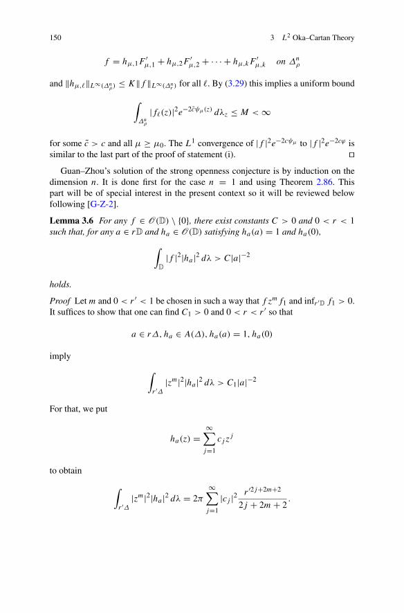
150 3 L2 Oka–Cartan Theory
f = hμ,1F′μ,1 + hμ,2F
′μ,2 + · · · + hμ,kF
′μ,k on Δn
ρ
and ‖hμ,�‖L∞(Δnρ)≤ K‖f ‖L∞(Δn
r )for all �. By (3.29) this implies a uniform bound
∫Δnρ
|f�(z)|2e−2cψμ(z) dλz ≤ M <∞
for some c > c and all μ ≥ μ0. The L1 convergence of |f |2e−2cψμ to |f |2e−2cϕ issimilar to the last part of the proof of statement (i). ��
Guan–Zhou’s solution of the strong openness conjecture is by induction on thedimension n. It is done first for the case n = 1 and using Theorem 2.86. Thispart will be of special interest in the present context so it will be reviewed belowfollowing [G-Z-2].
Lemma 3.6 For any f ∈ O(D) \ {0}, there exist constants C > 0 and 0 < r < 1such that, for any a ∈ rD and ha ∈ O(D) satisfying ha(a) = 1 and ha(0),
∫D
|f |2|ha|2 dλ > C|a|−2
holds.
Proof Let m and 0 < r ′ < 1 be chosen in such a way that f zmf1 and infr ′D f1 > 0.It suffices to show that one can find C1 > 0 and 0 < r < r ′ so that
a ∈ rΔ, ha ∈ A(Δ), ha(a) = 1, ha(0)
imply
∫r ′Δ|zm|2|ha|2 dλ > C1|a|−2
For that, we put
ha(z) =∞∑j=1
cj zj
to obtain
∫r ′Δ|zm|2|ha|2 dλ = 2π
∞∑j=1
|cj |2 r ′2j+2m+2
2j + 2m+ 2.

3.3 L2 Approaches to Analytic Ideals 151
Since∑∞
j=1 cj aj = 1 by assumption, we have
∞∑j=1
|cj |2 r ′2j+2m+2
2j + 2m+ 2≥( ∞∑j=1
2j + 2m+ 2
r ′2j+2m+2 |a|2j)−1
by the Cauchy–Schwarz inequality. Since
∞∑j=1
2j + 2m+ 2
r ′2j+2m+2 |a|2j =∣∣∣ ar ′∣∣∣2( (2m+ 2)r ′−2m−2
1− | ar ′ |2
+ 2r ′−2m−2
(1− | ar ′ |2)2
)
holds, C1 as above exists if 0 < 2r < r ′. ��Proof of the strong openness conjecture. Let F be a nonzero holomorphic functionon D satisfying
∫D
|F |2e−ϕ dλ <∞. (3.30)
We want to show that for some 0 < r < 1 and p > 1 it holds that∫rD|F |2e−pϕ dλ < ∞. Clearly, it suffices to show that by assuming ϕ < 0 and
F−1(0) = 0. By (3.30), there exists a sequence aj converging in D to 0 such that,ϕ(aj ) �= −∞ and
limj→∞ |aj |
2|F(aj )|2e−ϕ(aj ) = 0.
Therefore a sequence pj > 1 can be chosen so that
limj→∞ |aj |
2|F(aj )|2e−pjϕ(aj ) = 0
is satisfied. By Theorem 2.86, there exists a constant C > 0 such that, for each j
one can find Fj ∈ A(D) such that Fj (aj ) = F(aj ) and
∫Δ
|Fj |2e−pjϕ dλ ≤ C|F(aj )|2e−pjϕ(aj ). (3.31)
Taking pj closer to 1 if necessary, we may assume that
∫D
|Fj |2e−pjϕ dλ ≤ 2C|F(aj )|2e−ϕ(aj )
is satisfied. Since ϕ < 0, By (3.30) and (3.31),
limj→∞ |aj |
2∫D
|Fj |2 dλ = 0. (3.32)
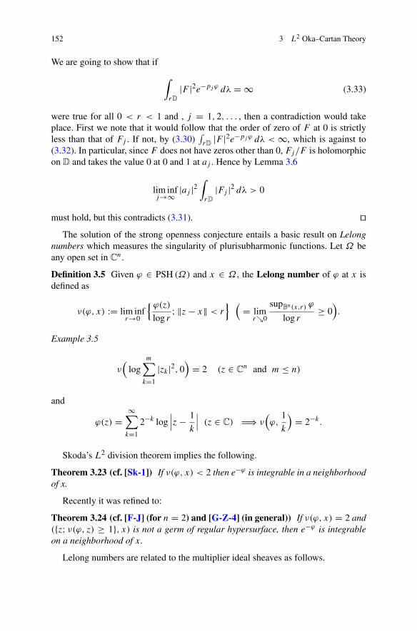
152 3 L2 Oka–Cartan Theory
We are going to show that if
∫rD
|F |2e−pjϕ dλ = ∞ (3.33)
were true for all 0 < r < 1 and , j = 1, 2, . . . , then a contradiction would takeplace. First we note that it would follow that the order of zero of F at 0 is strictlyless than that of Fj . If not, by (3.30)
∫rD|F |2e−pjϕ dλ <∞, which is against to
(3.32). In particular, since F does not have zeros other than 0, Fj/F is holomorphicon D and takes the value 0 at 0 and 1 at aj . Hence by Lemma 3.6
lim infj→∞ |aj |
2∫rD
|Fj |2 dλ > 0
must hold, but this contradicts (3.31). ��The solution of the strong openness conjecture entails a basic result on Lelong
numbers which measures the singularity of plurisubharmonic functions. Let Ω beany open set in C
n.
Definition 3.5 Given ϕ ∈ PSH (Ω) and x ∈ Ω , the Lelong number of ϕ at x isdefined as
ν(ϕ, x) := lim infr→0
{ ϕ(z)log r; ‖z− x‖ < r
} (= lim
r↘0
supBn(x,r) ϕ
log r≥ 0).
Example 3.5
ν(
logm∑k=1
|zk|2, 0)= 2 (z ∈ C
n and m ≤ n)
and
ϕ(z) =∞∑k=1
2−k log∣∣∣z− 1
k
∣∣∣ (z ∈ C) �⇒ ν(ϕ,
1
k
)= 2−k.
Skoda’s L2 division theorem implies the following.
Theorem 3.23 (cf. [Sk-1]) If ν(ϕ, x) < 2 then e−ϕ is integrable in a neighborhoodof x.
Recently it was refined to:
Theorem 3.24 (cf. [F-J] (for n = 2) and [G-Z-4] (in general)) If ν(ϕ, x) = 2 and({z; ν(ϕ, z) ≥ 1}, x) is not a germ of regular hypersurface, then e−ϕ is integrableon a neighborhood of x.
Lelong numbers are related to the multiplier ideal sheaves as follows.
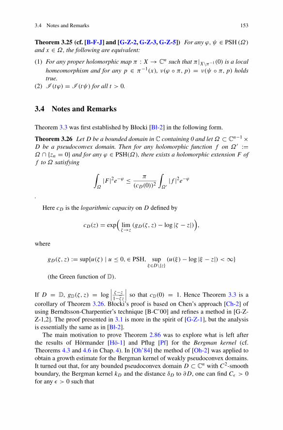
3.4 Notes and Remarks 153
Theorem 3.25 (cf. [B-F-J] and [G-Z-2, G-Z-3, G-Z-5]) For any ϕ,ψ ∈ PSH (Ω)
and x ∈ Ω , the following are equivalent:
(1) For any proper holomorphic map π : X→ Cn such that π |X\π−1(0) is a local
homeomorphism and for any p ∈ π−1(x), ν(ϕ ◦ π, p) = ν(ψ ◦ π, p) holdstrue.
(2) I (tϕ) = I (tψ) for all t > 0.
3.4 Notes and Remarks
Theorem 3.3 was first established by Błocki [Bł-2] in the following form.
Theorem 3.26 Let D be a bounded domain in C containing 0 and let Ω ⊂ Cn−1×
D be a pseudoconvex domain. Then for any holomorphic function f on Ω ′ :=Ω ∩ {zn = 0} and for any ϕ ∈ PSH(Ω), there exists a holomorphic extension F off to Ω satisfying
∫Ω
|F |2e−ϕ ≤ π
(cD(0))2
∫Ω ′|f |2e−ϕ
.
Here cD is the logarithmic capacity on D defined by
cD(z) = exp(
limζ→z
(gD(ζ, z)− log |ζ − z|)),
where
gD(ζ, z) := sup{u(ζ ) | u ≤ 0,∈ PSH, supξ∈D\{z}
(u(ξ)− log |ξ − z|) <∞}
(the Green function of D).
If D = D, gD(ζ, z) = log∣∣∣ ζ−z
1−ζz∣∣∣ so that cD(0) = 1. Hence Theorem 3.3 is a
corollary of Theorem 3.26. Błocki’s proof is based on Chen’s approach [Ch-2] ofusing Berndtsson-Charpentier’s technique [B-C’00] and refines a method in [G-Z-Z-1,2]. The proof presented in 3.1 is more in the spirit of [G-Z-1], but the analysisis essentially the same as in [Bł-2].
The main motivation to prove Theorem 2.86 was to explore what is left afterthe results of Hörmander [Hö-1] and Pflug [Pf] for the Bergman kernel (cf.Theorems 4.3 and 4.6 in Chap. 4). In [Oh’84] the method of [Oh-2] was applied toobtain a growth estimate for the Bergman kernel of weakly pseudoconvex domains.It turned out that, for any bounded pseudoconvex domain D ⊂ C
n with C2-smoothboundary, the Bergman kernel kD and the distance δD to ∂D, one can find Cε > 0for any ε > 0 such that

154 3 L2 Oka–Cartan Theory
C−1ε δD(z)
−2+ε < kD(z) < CεδD(z)−n−1 (3.34)
holds. The expected result was the inequality for ε = 0 (see (4.22) in Chap. 4),which had already been conjectured by Bergman. Since
kD(z) = sup{|f (z)|2; ‖f ‖2 = 1, f ∈ H 0,0(2) (D)}
(cf. (4.7) in Chap. 4), it is straightforward from Theorem 2.86 that (3.34) withε = 0 holds if ∂D is Lipschitz continuous in the sense that ∂D is locally thegraph of Lipschitz continuous function of 2n − 1 real variables. After establishingTheorem 2.86 in [Oh-T-1] and succeeding in removing ε from (3.34), the author hasbeen trying to generalize the result to extend its applications. Some of the materialsrelated to such activity will be reviewed below.
As was mentioned in Sect. 2.2.5, Skoda had already applied the L2 method tosolve a division problem with growth conditions (cf. Theorems 3.11 and 3.15).Skoda’s theory had applications to commutative algebra (cf. Theorem 3.16) andstimulated the introduction of an important notion of tight closure (see [L-T] and[H-S’06]). This was a big encouragement because there is an intimate relationbetween the division problem and the extension problem since the theory ofWeierstrass and Mittag–Leffler. More recently, this connection can be seen inCarleson’s solution [C’62] of Kakutani’s corona problem, a deep result of harmonicanalysis in one complex variable. Carleson established that, given any ideal I ofthe ring H∞ of bounded holomorphic functions on D generated by f1, . . . , fn,
I = H∞ holds if and only if infz∈D∑n
j=1 |fj (z)| > 0.1 In order to solve the coronaproblem, Carleson had to settle an extension problem in the following way.
Theorem 3.27 (cf. [C’58]) Let zk ∈ D (k = 1, 2, . . . ) be a sequence satisfying
infk
∏j �=k
∣∣∣ zk − zj
1− zj zk
∣∣∣ > 0.
Then the image of the map ρ : H∞ → CN defined by ρ(f )(k) = f (zk) coincides
with �∞ = {c ∈ CN; supk |c(k)| <∞}.
Theorem 3.26 was extended to a characterization of images of the restrictionmaps from Hp = {f ∈ O(D); ∫
D|f |p dλ < ∞} for 0 < p < ∞. (See [D’70] for
more detail.)In several variables, Skoda’s L2 division theory was followed by solutions of
extension problems under various growth conditions (cf. [N’80, Y’81, B-T’80, J’78,Dem’81]). For instance, an extension problem was solved in the following setting in[B-T’80] for application to questions of harmonic analysis (see also [B-S’89]): LetX be an analytic set in C
n and let p(z) ∈ PSH(Cn). First, for which holomorphic
1 T.Wolff gave an L2 proof to this theorem (cf. [K’80] and [G’80]).

3.4 Notes and Remarks 155
function f on X does there exist f ∈ O(Cn) satisfying f |X = f such that |f (z)| ≤C1exp(C2p(z)) holds for all z ∈ C
n for some constants C1 and C2? Secondly,under which condition on X is it true that for every holomorphic function f on Xsatisfying |f (z)| ≤ Aexp(Bp(z)), z ∈ X, there exists f ∈ O(Cn) satisfying theabove mentioned requirements? That the latter holds if X is algebraic follows fromresults of Ehrenpreis [E’70, chap.4] and Palamodov [P’70, chap.4].
As a result closer in the spirit of Carleson’s interpolation theorem for Hp, Beat-rous [B’85] proved an interpolation theorem on strongly pseudoconvex domainsby applying the method of integral kernels. Let D ⊂ C
n be a bounded stronglypseudoconvex domain, let S be a closed m-dimensional complex submanifold ofa neighborhood of D which intersects ∂D transversally and let D′ = S ∩ D. Fors > −1, p > 0, let Ap
s (X) = O(X) ∩ Lp(X, δsX dλ) for X = D or X = D′,where δX(z) = dist(z, ∂X) andLp(·, ·) denotes the Lebesgue space ofLp functions.Further, let Ap
−1(X) be the space of all holomorphic functions on X with boundaryvalues in Lp(∂X). Put A(X) =⋃A
ps (X) (s ≥ −1, p > 0).
Theorem 3.28 (cf. [B’85]) In the above situation the following hold.
(a) The restriction map R : O(D) → O(D′) maps Aps (D) continuously to
APn−m+s(D′).
(b) There exists a linear map
L : A(D′) −→ A(D)
which maps Apn−m+s(D′) continuously into A
ps (D) such that R(L(f )) = f
holds for all f .
The proof of Theorem 3.28 consists of finding a current T satisfying f T = 1 interms of the integral kernel of Henkin [H’70] and Ramirez [R’70].
The L2 method can be applied to extend Theorem 3.27. Let D be as above,let ϕ ∈ PSH(D) ∩ C0(D), let H be a smooth hypersurface in a neighborhood of Dwhich intersects ∂D transversally, and let Ap
α,ϕ be the space of f ∈ O(D) satisfying
∫D
e−ϕδα|f |pdλ <∞(
resp. limα↘−1
(α + 1)∫D
e−ϕδα|f |pdλ <∞)
for α > −1 (resp.α = −1) and p > 0.
Theorem 3.29 (cf. [Oh’03]) There exists a continuous linear map L : A20,ϕ(D ∩
H)→ A21,ϕ(D) such that L(f )|D∩H = f for all f .
Between [Oh-T-1] and [Oh’03], the author experienced a short period ofexcitement around 1993, when he found a partial answer to Suita’s conjecture in[Oh-16, Addendum] (see Chap. 4 for the detail of this problem). This discovery wasgreatly influenced by [Sp-1, Sp-2] and [S-W], which suggested the author what toexpect beyond (3.34). The following passage in the introduction to [Oh’94] reflectssuch a situation.

156 3 L2 Oka–Cartan Theory
Usually the conditions of interpolatability have been described in terms of highly analyticterms, like the convergence of a sequence associated to the Weierstrass canonical productor that of the Blaschke product. Generalizations to the several variables seem to have beendone in the same vein.
Nevertheless, the recent works of Seip and Wallstén show a remarkable similaritywith our previous results. Namely, they explored a more geometric concept of density tosolve certain interpolation problems, and the density is nothing but the curvature in manysituations, not to mention Einstein’s theory of gravity.
The manuscript of [Oh’94] was written while the author was staying at Harvarduniversity hosted by Yum Tong Siu. Einstein’s name is here probably because theauthor had a chance to talk in the seminar of Shing Tung Yau.
A primitive form of Theorem 3.5 was formulated in [Oh’94]. Since it may havesome instructive nature, let us present it here.
Let M be a Stein manifold equipped with a positive Radon measure dμM .By A2(M, dμM) we denote the set of holomorphic functions f on M satisfying‖f ‖2 := ∫
M|f |2 dμM <∞. Let S ⊂ M be a closed complex submanifold and let
dμS be a positive Radon measure on S. We say (S, dμS) is a set of interpolation forA2(M, dμM) if there exists a bounded linear operator
I : A2(S, dμS) −→ A2(M, dμM)
satisfying I (f )|S = f for all f . Let dk(z, S) denote the distance from z ∈ M to theunion of k-dimensional components of S, measured by any fixed Hermitian metricon M . A continuous function g : M → [−∞,∞) will be said to be a polarizationfunction of S if g is of class C2 outside g−1(−∞) and the function
g(z)− 2n−1∑k=0
(n− k) log dk(z, S)
is bounded on the compact subsets of M . Clearly the concept of the polarizationfunction does not depend on the metric. The set of polarization functions of S willbe denoted by Π(S).
We put
Πb(S) = {g ∈ Π(S); supM
g <∞}.
For any g ∈ Π(S) and for any volume form dVM on M , let dVM [g] be the minimalelement of the set of positive Radon measures dμ on S satisfying
∫S
f dμ ≥ lim supt→∞
∫M
f e−gχ{−t−1<g<−t} dVM
for all nonnegative continuous functions f with compact support on M . Here χAdenotes the characteristic function of the set A.

3.4 Notes and Remarks 157
Theorem 3.30 Let M be a Stein manifold equipped with a volume form dVM ofclass C2 and let S be a closed complex submanifold of M equipped with a positiveRadon measure dμ. Then (S, dμ) is a set of interpolation for A2(M, dVM) if thereexists a g ∈ Πb(S) such that dVM [g] ≤ dμ and
{ε; i(∂∂(1+ ε)g + κM) ≥ 0 on M \ S} ⊃ [0, ε0)
for some ε0 > 0. Here κM denotes the curvature form of dVM .
Another moment of excitement came when Siu gave a talk on [A-S] in March1995 at the first Hayama conference in complex analysis of several variables (cf.[Siu’96]). He gave an elegant application of Theorem 2.86 to the Fujita conjectureand gave an alternate proof with a better constant. In the same workshop the authorgave a survey talk presenting five types of applications of Theorem 2.86 and itsvariants. However, BEDFORD remarked that there are too many theorems in thetalk (cf. [Oh’96-2]). The author must admit that an application to Teichmüller spacesmight have been superfluous. In [Oh’96-1] it was shown by the L2 method thatTeichmüller spaces of Riemann surfaces can be biholomorphically nonequivalenteven if they are infinite dimensional. This answered a question raised by S. Mukai(personally to the author), but Earle and Gardiner [E-G’96], renowned experts ofTeichmüller theory, subsequently gave much better treatment of this problem.
It must be noted that one receives various error messages when one wants toextend Theorem 2.86 to other situations. The following example is in [Oh’05].
Example 3.6 Let D = B2(= B
2(0, 1)), let S = {(z, w) ∈ D; zw = 0} and let ϕk bea decreasing sequence of C∞ plurisubharmonic functions onD converging poitwiseto log |z− w|2. Then there exists no universal constant C such that, for any k andfor any holomorphic function f on S0 = S \ {(0, 0)} such that
∫S0e−ϕk |f |2 < ∞,
there exists a holomorphic extension fk of f to D satisfying
∫D
e−ϕk |fk|2 ≤ C
∫S0
e−ϕk |f |2.
Here the integrals are with respect to the Lebesgue measures. Indeed, if one takesthe function z(z − w)/(z + w) as f , a subsequence of such extensions fk wouldconverge to a holomorphic function f on D satisfying f (z, z) = 0, f (z, 0) = z andf (0, w) = 0, which is clearly impossible.
This example shows that Theorem 2.86 has no simple-minded generalization tocomplex spaces with singularities, unlike the case of Oka–Cartan theory. Absenceof the universal constant in the L2 extension has been more clearly shown by thefollowing result of Guan and Li [G-L’18]. It is remarkable that Skoda’s L2 divisiontheorem (Theorem 3.14 and Corollary 3.3) and the solution of Demailly’s strongopenness conjecture (cf. Theorem 3.22) are combined in the proof.

158 3 L2 Oka–Cartan Theory
Theorem 3.31 Let Ω ⊂ Cn (n ≥ 2) be a domain, A ⊂ Ω an analytic set through
the origin 0. Then, for sufficiently small balls Bn(0, r) ⊂ Ω , the L2 extension
theorem holds for (Bn(0, r), A) if and only if 0 is a regular point of A.
Proof It is enough to prove the necessity. Without loss of generality, we can assume1 ≤ dim0 A ≤ d ≤ n− 1, and the germ(A, 0) is irreducible, because the reduciblecase is easy as in the above example. Suppose that 0 is a singular point of A. Then,by applying the Weierstrass preparation theorem it is easy to see that there is a localcoordinate system (z′; z′′) = (z1, . . . , zd; zd+1, . . . , zn) around 0 such that for someconstant C > 0 we have ‖z′′‖ ≤ C‖z′‖ for any z ∈ A near 0. Let I ⊂ OA,0 bethe ideal generated by germs of holomorphic functions z1, . . . , zd ∈ OA,0, whereOA = OΩ/IA|A and zk are the residue classes of zk in OA,0. Since 0 is a singularityof A, there must exist d + 1 ≤ k0 ≤ n such that zk0 /∈ IA. Since ‖z′′‖ ≤ C‖z′‖for any z ∈ A near 0, |zk0 | ≤ C‖z′‖ and ‖z‖2 ≤ (1+ C2)‖z′‖2 on U ∩ A for someneighborhood U of 0.
On the other hand it is easy to verify that U can be chosen in such a way that
∫U∩Areg
‖z‖−2(d−1) dVA <∞
where dVA = ωd |Areg/d! and ω = i2
∑nk=1 dzk ∧ dzk , so that
∫U∩Areg
|zk0 |2‖z′‖−2ddVA ≤ C2(1+ C2)d−1∫U∩Areg
‖z‖−2(d−1)dVA <∞.
Thus, if the L2 extension theorem were true, there would exist a holomorphicfunction F ∈ O(Bn(0, r)) such that F |A = zk0 and
∫Bn(0,r)
|F |2‖z′‖−2d dλn <∞.
By Theorem 3.22, for sufficiently small ε > 0 and smaller Bn(0, r) we have
∫Bn(0,r)
|F |2‖z′‖−2(d+ε) dλn <∞.
Then we infer from Corollary 3.3 that there exist holomorphic functions fk ∈O(Bn(0, r)) such that F = ∑d
k=1 fkzk . By restricting to A we have zk0 ∈ I ,which contradicts zk0 /∈ I . ��
So the universal constant in the estimate for the L2 extension exists only for theextension from nonsingular sets. It must also be noted that the L2 extension canfail even for a fixed weight if functions must be extended from a hypersurface withsingularities (cf. [D-M’00]).
In [G-Z-1] Theorem 3.3 was further extended as follows.

3.4 Notes and Remarks 159
Theorem 3.32 For any pseudoconvex domain D ⊂ Cn, for any ϕ ∈ PSH(D), for
any ε > 0 and for any holomorphic function f on D′ = D ∩ {zn = 0}, there existsa holomorphic function f on D such that f |D′ = f and
∫D
|f |2(1+ |zn|2)1+ε e
−ϕ ≤ π
ε
∫D′|f |2e−ϕ.
There is a generalized variant of Theorem 3.32 in [G-Z’17] containing thefollowing.
Theorem 3.33 (see also [Oh’17]) Let α > 0. Then, in the situation of Theo-rem 3.32, every holomorphic function f on D′ extends to a holomorphic function fon D satisfying
∫D
e−α|zn|2−ϕ |f |2 ≤ π
α
∫D′e−ϕ |f |2.
Proof of Theorem 3.32 In Theorem 3.1 we put X = D, σ = zn, (B, b) = (D ×C, (1+ |zn|2)−1), (E, h) = (D×C, (1+ |zn|2)−1−εe−ϕ) and Q = ε−1(1+ |zn|2).Then, with respect to
s(t) = (1+ e−t )ε∫ t
−∞(1+ e−x)−ε dx,
u(t) = ε log (1+ e−t ),
φ(z) = −ε log (1+ |zn|2)
and
η(z) = s(log |zn|2),
similarly as in the proof of Theorem 3.3 one has
ηΘh − ∂∂η ≥ (su′′ − s′′)|t=log |zn|2 dzn ∧ dzn= −u′s′|t=log |zn|2 dzn ∧ dzn.
The semipositivity of the last term follows from u′ < 0 (obvious) and s′ ≥ 0. Thelatter inequality holds because
s′ =(eu∫ t
−∞e−u(x) dx
)′ = e2u((e−u)′
∫ t
−∞e−u(x) dx − e−2u
),
K := ((e−u)′)2 − (e−u)′′e−u = εe−t (1+ e−t )−2−2ε > 0

160 3 L2 Oka–Cartan Theory
and because the function r = ∫ t∞ e−u(x) dx satisfies
( r ′2 − r ′′rr ′
)′ = r(r ′′ − r ′′′r ′)r ′2
= rK
r ′2> 0.
Hence we are allowed to set c(z) = v(log |zn|2), where v = su′′−s′′s′2 . Finally
η + c−1 =(s + s′2
su′′ − s′′)∣∣∣
t=log |zn|2= 1
ε(1+ |zn|2),
since
s + s′2
su′′ − s′′= s − s′
u′= su′ − s′
u′= − 1
u′= 1
εet (1+ e−t ),
from which the conclusion follows immediately. ��For the proof of Theorem 3.33, we put
u(t) = eet
, s(t) = e−u(t)∫ t
−∞eu(x)dx
and apply Theorem 3.1 similarly to the above.As for other generalizations and refinements of Theorem 2.86, the reader is
referred to [M’93, P’05, M-V’07, M-V’17, B-L’16, H’17-1, H’17-2, C-D-M’17] and[Dem’17], for instance. Since some of them are based on a completely differenttechnology, the detail will be reviewed in Chap. 4 after some preliminaries on theBergman kernel.
SKODA once told the author that his method explained in 3.2.2 is quite naturaland satisfying. It was in 1984 when the author was trying to find what happens inCorollary 3.3 as ε → 0, with a hope to get some idea of proving Theorem 2.86.SKODA was right because the main ingredient of his theory is Lemma 3.3 whichremained untouchable in the L2 extension theory and around which a new develop-ment has been taking place. It was combined in [V’08] with (3.4) to yield anotherkind of refined L2 division theorems. The following is one of the recent results inthis direction. It extends Skoda’s theory by sacrificing the estimate of the solutions.
Theorem 3.34 (cf. [K’16]) Let X be a projective algebraic manifold, let L → X
be a holomorphic line bundle and let g1, . . . , gp ∈ H 0(X,L) be holomorphicsections (p ≥ 1). Let H → X be another holomorphic line bundle and let a and bbe singular fiber metrics on L and H , respectively, both with semipositive curvaturecurrent. Let q ≥ min (n, p − 1) be an integer, where n = dimX. If a holomorphicsection f ∈ H 0(X,O(KX ⊗H ⊗ L⊗(q+2))) satisfies
∫X
|f ∧ f |baq+2 |g|−2(q+1)a <∞,
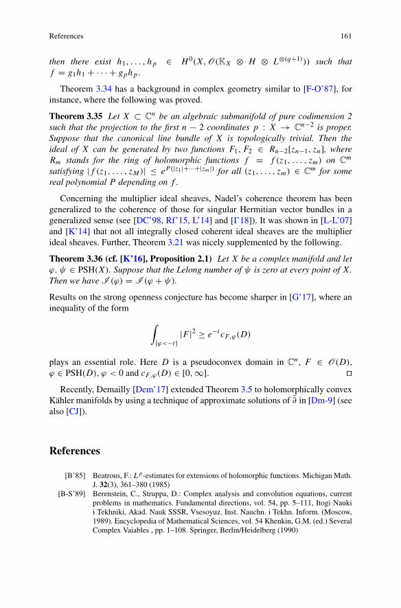
References 161
then there exist h1, . . . , hp ∈ H 0(X,O(KX ⊗ H ⊗ L⊗(q+1))) such thatf = g1h1 + · · · + gphp.
Theorem 3.34 has a background in complex geometry similar to [F-O’87], forinstance, where the following was proved.
Theorem 3.35 Let X ⊂ Cn be an algebraic submanifold of pure codimension 2
such that the projection to the first n − 2 coordinates p : X → Cn−2 is proper.
Suppose that the canonical line bundle of X is topologically trivial. Then theideal of X can be generated by two functions F1, F2 ∈ Rn−2[zn−1, zn], whereRm stands for the ring of holomorphic functions f = f (z1, . . . , zm) on C
m
satisfying |f (z1, . . . , zM)| ≤ eP (|z1|+···+|zm|) for all (z1, . . . , zm) ∈ Cm for some
real polynomial P depending on f .
Concerning the multiplier ideal sheaves, Nadel’s coherence theorem has beengeneralized to the coherence of those for singular Hermitian vector bundles in ageneralized sense (see [DC’98, Rf’15, L’14] and [I’18]). It was shown in [L-L’07]and [K’14] that not all integrally closed coherent ideal sheaves are the multiplierideal sheaves. Further, Theorem 3.21 was nicely supplemented by the following.
Theorem 3.36 (cf. [K’16], Proposition 2.1) Let X be a complex manifold and letϕ,ψ ∈ PSH(X). Suppose that the Lelong number of ψ is zero at every point of X.Then we have I (ϕ) = I (ϕ + ψ).
Results on the strong openness conjecture has become sharper in [G’17], where aninequality of the form
∫{ϕ<−t}
|F |2 ≥ e−t cF,ϕ(D)
plays an essential role. Here D is a pseudoconvex domain in Cn, F ∈ O(D),
ϕ ∈ PSH(D), ϕ < 0 and cF,ϕ(D) ∈ [0,∞]. ��Recently, Demailly [Dem’17] extended Theorem 3.5 to holomorphically convex
Kähler manifolds by using a technique of approximate solutions of ∂ in [Dm-9] (seealso [CJ]).
References
[B’85] Beatrous, F.: Lp-estimates for extensions of holomorphic functions. Michigan Math.J. 32(3), 361–380 (1985)
[B-S’89] Berenstein, C., Struppa, D.: Complex analysis and convolution equations, currentproblems in mathematics. Fundamental directions, vol. 54, pp. 5–111, Itogi Naukii Tekhniki, Akad. Nauk SSSR, Vsesoyuz. Inst. Nauchn. i Tekhn. Inform. (Moscow,1989). Encyclopedia of Mathematical Sciences, vol. 54 Khenkin, G.M. (ed.) SeveralComplex Vaiables , pp. 1–108. Springer, Berlin/Heidelberg (1990)
162 3 L2 Oka–Cartan Theory
[B-T’80] Berenstein, C., Taylor, B.: Interpolation problems in Cn with applications to
harmonic analysis. J. Anal. Math. 38, 188–254 (1980)[Brd’13] Berndtsson, B.: The openness conjecture for plurisubharmonic functions. arXiv:
1305.5781r1 [math.cv][B-C’00] Berndtsson, B., Charpentier, P.: A Sobolev mapping property of the Bergman Kernel.
Math. Z. 235(1), 1–10 (2000)[B-L’16] Berndtsson, B., Lempert, L.: A proof of the Ohsawa-Takegoshi theorem with sharp
estimates. J. Math. Soc. Jpn. 68(4), 1461–1472 (2016)[C-D-M’17] Cao, J.-Y., Demailly, J.-P., Matsumura, S.: A general extension theorem for coho-
mology classes on non reduced analytic subspaces. Sci. China Math. 60(6), 949–962(2017)
[C’58] Carleson, L.: An interpolation problem for bounded analytic functions. Am. J. Math.80, 921–930 (1958)
[C’62] Carleson, L.: Interpolations by bounded analytic functions and the corona problem.Ann. Math. 76(2), 547–559 (1962)
[Cl’07] Claudon, B.: Invariance for multiples of the twisted canonical bundle. Ann. Inst.Fourier (Grenoble) 57, 289–300 (2007)
[DC’98] de Cataldo, M.A.: Singular hermitian metrics on vector bundles. J. Reine Angew.Math. 502, 93–122 (1998)
[Dem’81] Demailly, J.-P.: Scindage holomorphe d’un morphisme de fibrés vectoriels semi-positifs avec estimations L2, Seminar Pierre Lelong-Henri Skoda (Analysis),1980/1981, and Colloquium at Wimereux, May 1981. Lecture Notes in Mathematics,vol. 919, pp. 77–107. Springer, Berlin/New York (1982)
[Dem’17] Demailly, J.-P.: Extension of holomorphic functions and cohomology classes fromnon reduced analytic subvarieties. In: The 12th Korean Conference on SeveralComplex Variables (KSCV12), July 2017, Gyeong-Ju, <hal-01660126>
[D-M’00] Diederich, K., Mazzilli, E.: A remark on the theorem of Ohsawa-Takegosh. NagoyaMath. J. 158, 185–189 (2000)
[D’70] Duren, P.: Theory of Hp spaces. In: Pure and Applied Mathematics, vol. 38,pp. xii+258. Academic, New York/London (1970)
[E-G’96] Earle, C., Gardiner, F.: Geometric isomorphisms between infinite-dimensionalTeichmüller spaces. Trans. Am. Math. Soc. 348(3), 1163–1190 (1996)
[E’70] Ehrenpreis, L.: Fourier analysis in several complex variables. In: Pure andApplied Mathematics, vol. XVII, pp. xiii+506. Wiley-Interscience Publishers, NewYork/London/Sydney (1970)
[F-O’87] Forster, O., Ohsawa, T.: Complete intersections with growth conditions. In: Alge-braic Geometry (Sendai, 1985). Advanced Studies in Pure Mathematics, vol. 10,pp. 91–104. North-Holland, Amsterdam (1987)
[G’80] Gamelin, T.W.: Wolff’s proof of the corona theorem. Israel J. Math. 37(1–2), 113–119 (1980)
[G’17] Guan, Q.-A.: A sharp effectiveness result of Demailly’s strong openness conjecture.arXiv: 1709.05880v4 [math.CV]
[G-L’18] Guan, Q.-A., Li, Z.-Q.: A characterization of regular points by Ohsawa-Takegoshiextension theorem. J. Math. Soc. Jpn. 70(1), 403–408 (2018)
[G-Z’17] Guan, Q.-A., Zhou, X.-Y.: Strong openness of multiplier ideal sheaves and optimalL2 extension. Sci. China Math. 60(6), 967–976 (2017)
[H’70] Henkin, G.M.: Integral representation of functions in strongly pseudoconvex regions,and applications to the ∂-problem. Mat. Sb. (N.S.) 82(124), 300–308 (1970)
[H’17-1] Hosono, G.: The optimal jet L2 extension of Ohsawa-Takegoshi type. arXiv:1706.08725v1 [math.CV]
[H’17-2] Hosono, G.: On sharper estimates of Ohsawa-Takegoshi L2-extension theorem.arXiv: 1708.08269v2 [math.CV]
[H-S’06] Huneke, C., Swanson, I.: Integral Closure of Ideals, Rings, and Modules. LondonMathematical Society Lecture Note Series, vol. 336, p. xiv+431. Cambridge Univer-sity Press, Cambridge (2006)

References 163
[I’18] Iwai, M.: Nadel-Nakano vanishing theorems of vector bundles with singular Hermi-tian metrics. arXiv: 1802.01794v1 [math.CV]
[J’78] Jennane, B.: Extension d’une fonction définie sur une sous-variété avec contrôle dela croissance. Séminaire Pierre Lelong-Henri Skoda (Analyse), Année 1976/1977.Lecture Notes in Mathematics, vol. 694, pp. 126–133. Springer, Berlin (1978)
[K’14] Kim, D.: The exactness of a general Skoda complex. Michigan Math. J. 63(1), 3–18(2014)
[K’16] Kim, D.: Skoda division of line bundle sections and pseudo-division. Int. J. Math.27(5), 1650042, 12 pp. (2016)
[K’80] Koosis, P.: Introduction to Hp-Spaces. With an Appendix on Wolff’s Proof of theCorona Theorem. London Mathematical Society Lecture Note Series, vol. 40, p.xv+376. Cambridge University Press, Cambridge/New York (1980)
[L-L’07] Lazarsfeld, R., Lee, K.: Local syzygies of multiplier ideals. Invent. Math. 167, 409–418 (2007)
[L’14] Lempert, L.: Modules of square integrable holomorphic germs. arXiv: 1404.0407v2[math.CV]
[M’93] Manivel, L.: Un théorème de prolongement L2 de sections holomorphes d’un fibréhermitien. Math. Z. 212(1), 107–122 (1993)
[M-V’07] McNeal, J., Varolin, D.: Analytic inversion of adjunction: L2 extension theoremswith gain. Ann. Inst. Fourier (Grenoble) 57(3), 703–718 (2007)
[M-V’17] McNeal, J., Varolin, D.: Extension of jets with L2 estimates, and an application.arXiv: 1707.04483v2 [math.CV]
[Nk’72] Nakamura, I.: On complex parallelisable manifolds and their small deformations.Proc. Jpn. Acad. 48, 447–449 (1972)
[N’80] Nishimura, Y.: Problème d’extension dans la théorie des fonctions entières d’ordrefini. J. Math. Kyoto Univ. 20(4), 635–650 (1980)
[Oh’84] Ohsawa, T.: Boundary behavior of the Bergman kernel function on pseudoconvexdomains. Publ. Res. Inst. Math. Sci. 20(5), 897–902 (1984)
[Oh’94] Ohsawa, T.: On the extension of L2 holomorphic functions. IV. A new densityconcept. In: Mabuchi, T., et al. (eds.) Geometry and Analysis on Complex Manifolds,pp. 157–170. World Scientific Publishing, River Edge (1994)
[Oh’96-1] Ohsawa, T.: On the analytic structure of certain infinite-dimensional Teichmüllerspaces. Nagoya Math. J. 141, 143–156 (1996)
[Oh’96-2] Ohsawa, T.: Applications of L2 estimates and some complex geometry. In: Noguchi,J. (ed.) Geometric Complex Analysis (Hayama, 1995), pp. 505–523. World ScientificPublishing, River Edge (1996)
[Oh’03] Ohsawa, T.: On the extension of L2 holomorphic functions. VI. A limiting case. In:Explorations in Complex and Riemannian Geometry. Contemporary Mathematics,vol. 332, pp. 235–239. American Mathematical Society, Providence (2003)
[Oh’05] Ohsawa, T.: On a curvature condition that implies a cohomology injectivity theoremof Kollár-Skoda type. Publ. Res. Inst. Math. Sci. 41(3), 565–577 (2005)
[Oh’17] Ohsawa, T.: On the extension of L2 holomorphic functions VIII–a remark on atheorem of Guan and Zhou. Internat. J. Math. 28(9), 1740005, 12 (2017)
[P’70] Palamodov, V.: Linear differential operators with constant coefficients. Translatedfrom the Russian by Brown, A.A. Die Grundlehren der mathematischen Wis-senschaften, Band 168, p. viii+444. Springer, New York/Berlin (1970)
[P’05] Popovici, D.: L2 extension for jets of holomorphic sections of a Hermitian linebundle. Nagoya Math. J. 180, 1–34 (2005)
[R’70] Ramírez de, A.E.: Ein Divisionsproblem und Randintegraldarstellungen in derkomplexen Analysis. Math. Ann. 184, 172–187 (1969/1970)
[Rf’15] Raufi, H.: Singular hermitian metrics on holomorphic vector bundles. Ark. Mat.53(2), 359–382 (2015)

164 3 L2 Oka–Cartan Theory
[Siu’96] Siu, Y.-T.: The Fujita Conjecture and the Extension Theorem of Ohsawa-Takegoshi.Geometric Complex Analysis (Hayama, 1995), pp. 577–592. World ScientificPublishing, River Edge (1996)
[Siu’02] Siu, Y.-T.: Extension of twisted pluricanonical sections with plurisubharmonicweight and invariance of semipositively twisted plurigenera for manifolds notnecessarily of general type. In: Complex Geometry (Göttingen, 2000), pp. 223–277.Springer, Berlin (2002)
[Ty’06] Takayama, S.: Pluricanonical systems on algebraic varieties of general type. Invent.Math. 165(3), 551–587 (2006)
[T’02] Tsuji, H.: Deformation invariance of plurigenera. Nagoya Math. J. 166, 117–134(2002)
[V’08] Varolin, D.: Division theorems and twisted complexes. Math. Z. 259, 1–20 (2008)[Y-Z’15] Ye, F., Zhu, Z.-X.: On Fujita’s conjecture in dimension 5. arXiv: 1511.09154v1
[Y’81] Yoshioka, T.: Cohomologie à estimation L2 avec poids plurisousharmoniques etextension des fonctions holomorphes avec contrôle de la croissance. Osaka J. Math.19(4), 787–813 (1982)
Chapter 4Bergman Kernels
Abstract Applications of the L2 method to the Bergman kernels will be discussed.Emphasis is put on the results obtained in recent decades. Among them, there arevarious estimates for the Bergman kernel from below on weakly pseudoconvexdomains, including the solution of a long-standing conjecture of Suita by Błocki(Invent Math 193:149–158, 2013) and Guan and Zhou (Ann Math 181:1139–1208,2015). Recently discovered variational properties due to Maitani and Yamaguchi(Math Ann 330:477–489, 2004) and Berndtsson (Ann Inst Fourier (Grenoble)56(6):1633–1662, 2006; Ann Math 169:531–560, 2009) are also discussed. In abroader framework, they are describing the parameter dependence of the Bergmankernels associated to families or sequences of complex manifolds and vectorbundles. Most of these new results are closely related to the L2 extension theoremsin the previous chapter. Among them, a surprise is that a variational property ofthe relative canonical bundles generalizing that of the Bergman kernels, whichoriginally belongs to the theory of variation of Hodge structures, happens to implyan optimal L2 extension theorem (cf. Berndtsson and Lempert, J Math Soc Jpn68:1461–1472, 2016.
4.1 Bergman Kernel and Metric
The Bergman kernel, named after Stefan Bergman (1895–1977), is by definitionthe reproducing kernel of the space of L2 holomorphic n-forms on connected n-dimensional complex manifolds. Its significance in complex geometry has beengradually understood through many spectacular works in the last century. Forinstance, C. Fefferman [F] analyzed the boundary behavior of the Bergman kernelon strongly pseudoconvex domains with C∞ boundary, and proved that anybiholomorphic map between such bounded domains in C
n extends smoothly to adifffeomorphism between their closures. Recently, methods for analyzing certaingeneralized Bergman kernels have brought new insights into some aspects ofalgebraic geometry and differential geometry (cf. [Siu-7, Siu-9, Siu-10, Siu-11,Siu-12, B-Pa, Ds] and [Ma]). The purpose of this chapter is to review some of theresults on the Bergman kernels related to such a new development.
© Springer Japan KK, part of Springer Nature 2018T. Ohsawa, L2 Approaches in Several Complex Variables, SpringerMonographs in Mathematics, https://doi.org/10.1007/978-4-431-56852-0_4
165
166 4 Bergman Kernels
Since it seems worthwhile to recognize the surroundings of the Bergman kernelin complex analysis and its connection to various concepts, let us briefly reviewsome history here.
The circle division theory of C.F. Gauss (1777–1855), which was discoveredon 3/30/1796 is a giant leap in mathematics and the first step towards complexgeometry. In the early nineteenth century, it brought new progress in the theoryof elliptic integrals. It had been developed by L. Euler (1707–1783) and A.-M. Legendre (1752–1833) as an art of change of variables in their integration.Inspired by the work of Gauss, N.-H. Abel (1802–1829) was led at first to algebraicinsolvability of equations of degree 5, and subsequently discovered that the inversefunctions of elliptic integrals are nothing but doubly periodic analytic functions inone complex variable, i.e. elliptic functions. He eventually reached a remarkablecharacterization of principal divisors in the theory of algebraic functions of onevariable (Abel’s theorem). The latter is now regarded as the starting point ofalgebraic geometry. As a generalization of Abel’s theory on elliptic functions, thetheory of multiply periodic functions in several variables was developed by G.Jacobi (1804–1851), K. Weierstrass (1815–1897) and B. Riemann (1826–1866). Onthe other hand, in spite of an important contribution of H. Poincaré (1854–1912)on normal functions and a subsequent work of S. Lefschetz (1884–1972), it wasnot before the appearance of the theory of harmonic integrals on Kähler manifoldsby W.V.D. Hodge (1903–1975) that Abel’s idea became really efficient in severalvariables (cf. [Ho]). This delay is, to the author’s opinion, mainly because of the lackof the viewpoint of orthogonal projection in Hilbert spaces. Recall that it was onlyin 1899 that D. Hilbert (1862–1943) awoke Riemann’s idea of Dirichlet’s principlefrom a deep sleep (cf. [R-2]) and that the basic representation theorem of F. Riesz(1880–1956), which is often crucial in the existence proofs under orthogonalityconditions, was not available until 1907. History shows that such a systematicconstruction in abstract mathematics emerged only after the detailed studies oforthogonal polynomials in the nineteenth century. It culminated in a general methodof orthogonal projection by H. Weyl (1885–1955). Weyl’s method (cf. [Wy-1])became the analytic base of Hodge’s theory, which was later combined with analyticsheaf theory by K. Kodaira [K-2, K-3] and developed into the method presented inChap. 2. That Weyl anticipated a lot in this method is modestly suggested in [Wy-2].Anyway, the Bergman kernel came into the picture around 1922 (cf. [Be] and [Bo])in such a circumstance.
4.1.1 Bergman Kernels
For any set S, the set of C-valued functions on S, simply denoted by CS , is naturally
equipped with the structure of a complex vector space. A subspace of CS , say H
equipped with an inner product is called a reproducing kernel Hilbert space if thefollowing conditions are satisfied.
4.1 Bergman Kernel and Metric 167
(i) H is complete with respect to the associated norm.(ii) For any element x of S, the map [x] from H to C defined by [x](f ) = f (x) is
continuous.
Given a reproducing kernel Hilbert space H , Riesz’s representation theoremimplies that there exists uniquely a function on S × S say KH , satisfying thefollowing:
(a) KH(∗, y) ∈ H for any y.(b) (u,KH (∗, y)) = u(y) for any u ∈ H and y ∈ S.
We shall say that KH is the reproducing kernel of H .Among such H and KH , some deserve special attention when S has certain
structures as manifolds or groups. For our purpose, an important example is thecase where S is a complex manifold M equipped with a Hermitian metric and H isH
0,0(2) (M), the space of L2 holomorphic functions on M .
This way of regardingH 0,0(2) (M) as a reproducing kernel Hilbert space is naturally
generalized for the space of L2 holomorphic sections of Hermitian holomorphicvector bundles over M , replacing [x] in (ii) by the evaluation of the sections of E atx. Accordingly, for any Hermitian holomorphic vector bundle E over a Hermitianmanifold M , or more generally for any holomorphic vector bundle with a singularfiber metric over a Hermitian manifold, H 0,0
(2) (M,E) has a reproducing kernel as a
section of p∗1E⊗p∗2E. Here pj denotes the projection to the j -th factor of M ×M .
Note that the spaces H 0,0(2) (M,E) are separable, so that they are isomorphic to
�2C:={(cj )
∞j=1; cj ∈ C and
∞∑j=1
|cj |2 <∞}
if dimH0,0(2) (M,E) = ∞. An important special case is when E is the canonical
bundle KM of M . In this situation H0,0(2) (M,E) = H
n,0(2) (M) if M is of pure
dimension n, and the inner product of the space is independent of the choices of themetric on M as long as the fiber metric of the canonical bundle is induced from themetric on M . More explicitly, Hn,0
(2) (M) is equipped with a canonical inner product
2−nin2∫M
u ∧ v. (4.1)
The reproducing kernel of Hn,0(2) (M) with respect to this inner product is called
the Bergman kernel of M , denoted by KM instead of KHn,0(2) (M)
for simplicity.
A question of basic interest is how KM detects the geometry of M . Some of theproperties of KM follow immediately from the definition. For instance, it is clearthat
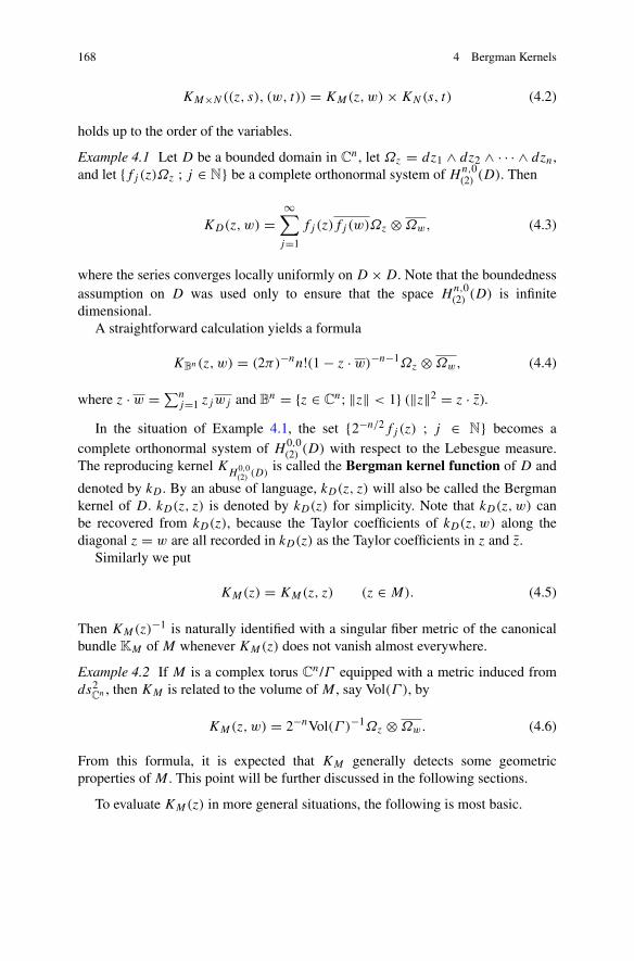
168 4 Bergman Kernels
KM×N((z, s), (w, t)) = KM(z,w)×KN(s, t) (4.2)
holds up to the order of the variables.
Example 4.1 Let D be a bounded domain in Cn, let Ωz = dz1 ∧ dz2 ∧ · · · ∧ dzn,
and let {fj (z)Ωz ; j ∈ N} be a complete orthonormal system of Hn,0(2) (D). Then
KD(z,w) =∞∑j=1
fj (z)fj (w)Ωz ⊗Ωw, (4.3)
where the series converges locally uniformly on D ×D. Note that the boundednessassumption on D was used only to ensure that the space H
n,0(2) (D) is infinite
dimensional.A straightforward calculation yields a formula
KBn(z, w) = (2π)−nn!(1− z · w)−n−1Ωz ⊗Ωw, (4.4)
where z · w =∑nj=1 zjwj and B
n = {z ∈ Cn; ‖z‖ < 1} (‖z‖2 = z · z).
In the situation of Example 4.1, the set {2−n/2fj (z) ; j ∈ N} becomes acomplete orthonormal system of H 0,0
(2) (D) with respect to the Lebesgue measure.The reproducing kernel K
H0,0(2) (D)
is called the Bergman kernel function of D and
denoted by kD . By an abuse of language, kD(z, z) will also be called the Bergmankernel of D. kD(z, z) is denoted by kD(z) for simplicity. Note that kD(z,w) canbe recovered from kD(z), because the Taylor coefficients of kD(z,w) along thediagonal z = w are all recorded in kD(z) as the Taylor coefficients in z and z.
Similarly we put
KM(z) = KM(z, z) (z ∈ M). (4.5)
Then KM(z)−1 is naturally identified with a singular fiber metric of the canonical
bundle KM of M whenever KM(z) does not vanish almost everywhere.
Example 4.2 If M is a complex torus Cn/Γ equipped with a metric induced from
ds2Cn , then KM is related to the volume of M , say Vol(Γ ), by
KM(z,w) = 2−nVol(Γ )−1Ωz ⊗Ωw. (4.6)
From this formula, it is expected that KM generally detects some geometricproperties of M . This point will be further discussed in the following sections.
To evaluate KM(z) in more general situations, the following is most basic.

4.1 Bergman Kernel and Metric 169
Proposition 4.1
KM(z) = sup{σ(z)⊗ σ(z); ‖σ‖2 = 1, σ ∈ Hn,0(2) (M)} (4.7)
holds for any z ∈ M . Here the right-hand side of (4.7) is understood to be zero ifH
n,0(2) (M) = {0}.
Corollary 4.1 For any open set U ⊂ M , KU(z) ≥ KM(z) holds for any z ∈ U .
It is also of basic importance that sup{|f (z)|2; ‖f ‖2 = 1, f ∈ H0,0(2) (D)} is
attained by kD(∗, z)/√kD(z), and that KUj (z,w) converges to KM(z,w) locallyuniformly on M ×M if Uj increasingly converges to M .
4.1.2 The Bergman Metric
Let Mj (j = 1, 2) be two complex manifolds of pure dimension n. Suppose thatthere exists a biholomorphic map f : M1 → M2. Then f induces an isometrybetween Hn,0
(2) (Mj ) by the pull-back of (n, 0)-forms. Accordingly,
KM1 = f ∗KM2 . (4.8)
In terms of the local coordinates ζ1 around p ∈ M1 and ζ2 around q ∈ M2 such thatf (p) = q, the relation (4.8) is explicitly written as
k1(ζ1) = k2(f (ζ1))| det(∂ζ2/∂ζ1)|2, (4.9)
where KMj(z) = kj (ζj )Ωζj ⊗ Ωζj . Therefore, if KMj
(z) are nowhere zero, thecurvature forms θj of KMj
(z)−1 also satisfy the relation
θ1 = f ∗θ2. (4.10)
In particular, if θj =∑nα,β=1 θjαβ dζ
αj ∧dζβj , and (θjαβ) are everywhere positive
definite, f is an isometry with respect to the metrics
n∑α,β=1
θjαβ dζαj ⊗ dζ
βj , (4.11)
which are called the Bergman metrics of Mj . Here the notation for the metric is asa fiber metric of a holomorphic tangent bundle. The Bergman metric of a complexmanifold M will be denoted by ds2
M,b. Equation (4.10) means that biholomorphicmaps preserve the Bergman metrics.

170 4 Bergman Kernels
Example 4.3
ds2Bn,b = (1− ‖z‖2)−1 ds2
Cn + (1− ‖z‖2)−2∂‖z‖2 ⊗ ∂‖z‖2, (4.12)
where ds2Cn =∑n
j=1 dzj ⊗ dzj . (ds2Cn,b
does not exist.)
For a bounded domain D in Cn, the Bergman metric ds2
D,b will be identified with
∂∂ log kD(z) by an abuse of notation. In terms of the notation (4.2),
ds2D,b = ∂∂ log kD(z) = k−1
D ∂∂kD − k−2D ∂kD∂kD
= (∑|fj |2)−2
∑j �=k
(fj ∂fk − fk∂fj )(fj ∂fk − fk∂fj ), (4.13)
where ∧ and ⊗ are omitted to avoid confusion.Consequently, ds2
D,b is characterized as follows.
Proposition 4.2 ds2D,b = ι∗ds2
CP∞ , where CP
∞ is the quotient of �2C\ {0} by C
∗,ds2
CP∞ is induced from ds2
�2C
, and ι(z) = (f1(z) : f2(z) : · · · ).
For any bounded domain D ⊂ Cn, z0 ∈ D and ξ ∈ T 1.0
z0D, we put
b(ξ) = sup{|ξf |; f ∈ H 0,0(2) (D), f (z0) = 0, ‖f ‖ = 1}. (4.14)
Another immediate consequence of (4.13) is:
Proposition 4.3 In the above situation, the length of ξ with respect to ds2D,b is
b(ξ)/√kD(z0). (4.15)
4.2 The Boundary Behavior
Among the analytic properties of the Bergman kernels which reflect the geometryof complex manifolds, the boundary behavior is studied from various viewpoints.Since it is often hard to calculate the Bergman kernels explicitly, description ofprincipal terms of their singularities and their asymptotic expansions is aimed at. Itis expected that this can be achieved in terms of geometric quantities such as theLevi form of the boundary and the curvature form of the bundles. The L2 methodfor the ∂ operator is available to localize the problem. It was first applied in the caseof strongly pseudoconvex domains by Hörmander [Hö-1]. To estimate the Bergmankernels from below on weakly pseudoconvex domains, the L2 extension theorem(Theorem 3.3) is useful.
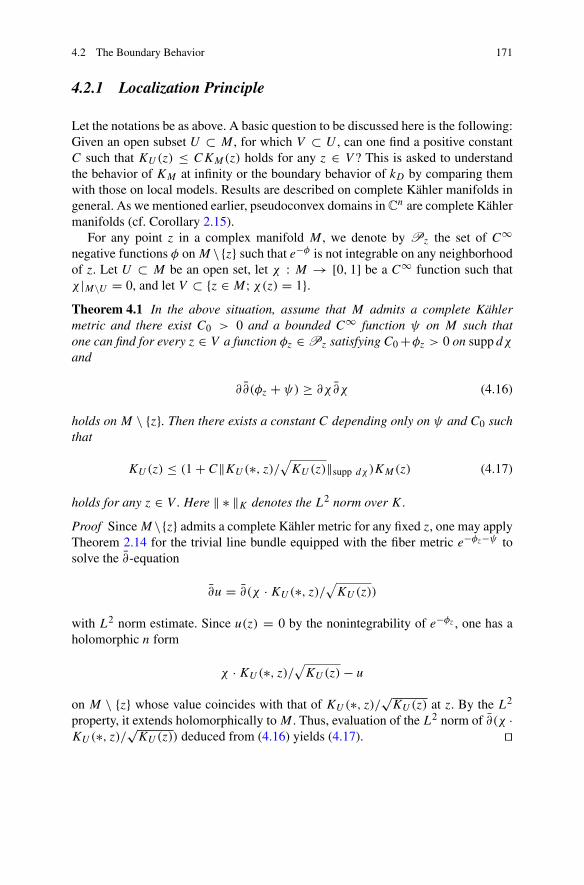
4.2 The Boundary Behavior 171
4.2.1 Localization Principle
Let the notations be as above. A basic question to be discussed here is the following:Given an open subset U ⊂ M , for which V ⊂ U , can one find a positive constantC such that KU(z) ≤ CKM(z) holds for any z ∈ V ? This is asked to understandthe behavior of KM at infinity or the boundary behavior of kD by comparing themwith those on local models. Results are described on complete Kähler manifolds ingeneral. As we mentioned earlier, pseudoconvex domains in C
n are complete Kählermanifolds (cf. Corollary 2.15).
For any point z in a complex manifold M , we denote by Pz the set of C∞negative functions φ on M \{z} such that e−φ is not integrable on any neighborhoodof z. Let U ⊂ M be an open set, let χ : M → [0, 1] be a C∞ function such thatχ |M\U = 0, and let V ⊂ {z ∈ M;χ(z) = 1}.Theorem 4.1 In the above situation, assume that M admits a complete Kählermetric and there exist C0 > 0 and a bounded C∞ function ψ on M such thatone can find for every z ∈ V a function φz ∈Pz satisfying C0+φz > 0 on supp dχand
∂∂(φz + ψ) ≥ ∂χ∂χ (4.16)
holds on M \ {z}. Then there exists a constant C depending only on ψ and C0 suchthat
KU(z) ≤ (1+ C‖KU(∗, z)/√KU(z)‖supp dχ )KM(z) (4.17)
holds for any z ∈ V . Here ‖ ∗ ‖K denotes the L2 norm over K .
Proof Since M \{z} admits a complete Kähler metric for any fixed z, one may applyTheorem 2.14 for the trivial line bundle equipped with the fiber metric e−φz−ψ tosolve the ∂-equation
∂u = ∂(χ ·KU(∗, z)/√KU(z))
with L2 norm estimate. Since u(z) = 0 by the nonintegrability of e−φz , one has aholomorphic n form
χ ·KU(∗, z)/√KU(z)− u
on M \ {z} whose value coincides with that of KU(∗, z)/√KU(z) at z. By the L2
property, it extends holomorphically to M . Thus, evaluation of the L2 norm of ∂(χ ·KU(∗, z)/√KU(z)) deduced from (4.16) yields (4.17). ��

172 4 Bergman Kernels
Corollary 4.2 Let D be a bounded pseudoconvex domain in Cn, let z0 ∈ ∂D and
let Uj (j = 1, 2) be neighborhoods of z0 in Cn such that U1 � U2. Then there exists
C > 0 such that
C−1kD(z) < kU2∩D(z) < CkD(z) (4.18)
holds for any z ∈ U1 ∩D.
Corollary 4.3 Let D be a pseudoconvex domain in Cn, let z0 ∈ ∂D, and let U be
a neighborhood of z0. Suppose that ∂D is strongly pseudoconvex at z0. Then
limz→z0
kU∩D(z)/kD(z) = 1. (4.19)
In view of the proof of Theorem 4.1, it is easy to see that a similar localizationprinciple holds for the Bergman metric.
Proposition 4.4 In the situation of Corollary 4.2, there exists C > 0 such that
C−1bD(ξ) < bU2∩D(ξ) < CbD(ξ) (4.20)
holds for any ξ ∈ T 1,0z C
n with z ∈ U1 ∩D.
Combining Propositions 4.3 and 4.4 with Corollary 4.2, we obtain:
Theorem 4.2 In the situation of Corollary 4.2, there exists C > 0 such that
C−1 ds2D,b < ds2
U2∩D,b < C ds2d,b (4.21)
holds on U1 ∩D.
4.2.2 Bergman’s Conjecture and Hörmander’s Theorem
Let us start from a naïve observation. Let D be a bounded domain in Cn and let
z0 ∈ ∂D. Assume that there exist domains Dj ⊂ Cn(j = 1, 2) with D1 ⊂ D ⊂ D2
such that there exist biholomorphic authomorphisms αj (j = 1, 2) of Cn satisfyingα1(D1) = B
n, α2(D2) = Dn, α1(z0) ∈ ∂Bn and α2(z0) ∈ ∂D × D
n−1. Then onecan find C > 0 such that
C−1δD(z)−2 < kD(z) < CδD(z)
−n−1 (4.22)
if z ∈ D and ‖z − z0‖ < δD(z). Recall that δD(z) denotes the Euclidean distancefrom z to ∂D. In view of this, Bergman conjectured (or even asserted) that theestimate (4.22) is valid for any bounded pseudoconvex domain with C2-smoothboundary (cf. [B-T]). Note that the existence of D1 as above is obvious, but D2
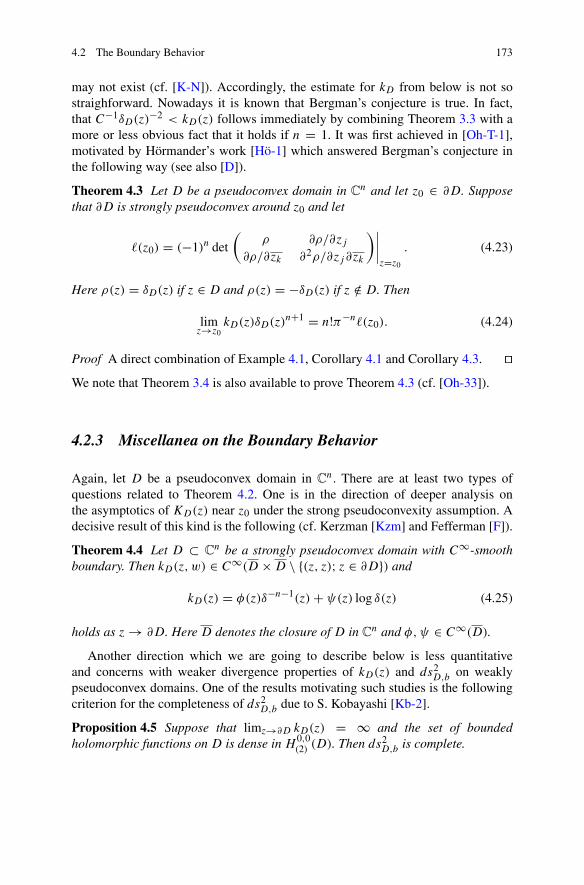
4.2 The Boundary Behavior 173
may not exist (cf. [K-N]). Accordingly, the estimate for kD from below is not sostraighforward. Nowadays it is known that Bergman’s conjecture is true. In fact,that C−1δD(z)
−2 < kD(z) follows immediately by combining Theorem 3.3 with amore or less obvious fact that it holds if n = 1. It was first achieved in [Oh-T-1],motivated by Hörmander’s work [Hö-1] which answered Bergman’s conjecture inthe following way (see also [D]).
Theorem 4.3 Let D be a pseudoconvex domain in Cn and let z0 ∈ ∂D. Suppose
that ∂D is strongly pseudoconvex around z0 and let
�(z0) = (−1)n det
(ρ ∂ρ/∂zj
∂ρ/∂zk ∂2ρ/∂zj ∂zk
)∣∣∣∣z=z0
. (4.23)
Here ρ(z) = δD(z) if z ∈ D and ρ(z) = −δD(z) if z /∈ D. Then
limz→z0
kD(z)δD(z)n+1 = n!π−n�(z0). (4.24)
Proof A direct combination of Example 4.1, Corollary 4.1 and Corollary 4.3. ��We note that Theorem 3.4 is also available to prove Theorem 4.3 (cf. [Oh-33]).
4.2.3 Miscellanea on the Boundary Behavior
Again, let D be a pseudoconvex domain in Cn. There are at least two types of
questions related to Theorem 4.2. One is in the direction of deeper analysis onthe asymptotics of KD(z) near z0 under the strong pseudoconvexity assumption. Adecisive result of this kind is the following (cf. Kerzman [Kzm] and Fefferman [F]).
Theorem 4.4 Let D ⊂ Cn be a strongly pseudoconvex domain with C∞-smooth
boundary. Then kD(z,w) ∈ C∞(D ×D \ {(z, z); z ∈ ∂D}) and
kD(z) = φ(z)δ−n−1(z)+ ψ(z) log δ(z) (4.25)
holds as z→ ∂D. Here D denotes the closure of D in Cn and φ,ψ ∈ C∞(D).
Another direction which we are going to describe below is less quantitativeand concerns with weaker divergence properties of kD(z) and ds2
D,b on weaklypseudoconvex domains. One of the results motivating such studies is the followingcriterion for the completeness of ds2
D,b due to S. Kobayashi [Kb-2].
Proposition 4.5 Suppose that limz→∂D kD(z) = ∞ and the set of boundedholomorphic functions on D is dense in H 0,0
(2) (D). Then ds2D,b is complete.

174 4 Bergman Kernels
Proof Let z0 ∈ D and let γ : [0, 1) → D be a C∞ curve with γ (0) = z0 andγ (t) → ∂D as t → 1. Then, by the assumption on H 0,0
(2) (D), one can find for anyε > 0 a bounded holomorphic function f on D such that
|f (z0)|2 = kD(z0) and∥∥∥f − kD(z, z0)√
kD(z0)
∥∥∥ < ε.
Hence, since kD(z) explodes at the boundary, one can find t0 and an isometricembedding ι : D → P
∞C(:= C
N \ {0}/C∗) such that ι(z0) = (1 : 0 : 0 · · · )and ι(γ (t0)) = (0 : 1 : · · · ). Hence ds2
D,b is complete. ��Kobayashi also proved that any bounded analytic polyhedron satisfies the assump-tions of Proposition 4.5.
Theorem 4.5 (cf. [Kb-1]) Let P1, . . . , Pm be polynomials in z = (z1, . . . , zn) andlet D ⊂ C
n be a bounded connected component of {z; |Pj (z)| < 1, 1 ≤ j ≤ m}.Then limz→∂D kD(z) = ∞ and ds2
D,b is complete.
Applying Skoda’s L2 division theorem, P. Pflug [Pf] obtained the following.
Theorem 4.6 Let D ⊂ Cn be a bounded pseudoconvex domain and let z0 ∈ ∂D.
Assume that there exist α > 0 and a sequence {pμ}∞μ=1 ⊂ Cn \ D converging
to z0 such that {z; ‖z − pμ‖ < ‖z0 − pμ‖α} ⊂ Cn \ D for all μ ∈ N. Then
limz→z0 kD(z) = ∞.
Pflug’s theorem suggests that kD(z) will explode along ∂D under some weakregularity assumption on ∂D. A natural class to be studied has existed for a long timein potential theory (cf. [Wn, Bou]). As a class of complex manifolds it is defined asfollows.
Definition 4.1 A complex manifold M is said to be hyperconvex if there exists abounded strictly plurisubharmonic exhaustion function on M .
Diederich and Fornaess [D-F-1] proved that any bounded pseudoconvex domainin C
n with C2 smooth boundary is hyperconvex. Kerzman and Rosay [K-R]generalized the result to the C1 smooth case. The following simple observation isuseful.
Proposition 4.6 M is hyperconvex if and only if there exists a strictly plurisub-harmonic exhaustion function ϕ on M satisfying ∂∂ϕ ≥ c∂ϕ∂ϕ for some positiveconstant c.
Proof Let φ be a bounded strictly plurisubharmonic exhaustion function on M suchthat supM φ = 0. Then
∂∂(− log (−φ)) = ∂∂φ
−φ +∂φ∂φ
φ2 ≥ ∂(log (−φ))∂(log (−φ)).

4.2 The Boundary Behavior 175
Conversely, if ∂∂ϕ ≥ c∂ϕ∂ϕ for some positive constant c, one can find a boundedincreasing function λ such that λ(ϕ) is a strictly plurisubharmonic exhaustionfunction on M . ��By virtue of the detailed study of homogeneous domains (cf. [PS]), homogeneousbounded domains are known to be hyperconvex (cf. [K-Oh]). Based on Bers’srealization of Teichmüller spaces as bounded domains in C
n, Krushkal’ [Kr] showedthat any finite-dimensional Teichmüller space is hyperconvex. When dimM = 1,hyperconvexity of M is equivalent to the exhaustiveness of the Green function ofM (cf. Proposition 3 in [Oh-16]), which can be seen easily from the definition ofthe Green function. Recall that the Green function of a Riemann surface M is bydefinition the maximal element of the set of continuous functions g : M ×M →[−∞, 0) such that, for each point w ∈ M , g(z,w) is subharmonic in z and, for anylocal coordinate ζ around w, g(z,w) − log |ζ | is bounded on {z; 0 < |ζ(z)| < 1}.The Green function of M will be denoted by gM if it exists. Otherwise we putgM ≡ −∞ for the convenience of the notation.
Example 4.4
gD(z, w) = log∣∣∣ z− w
1− zw
∣∣∣.
Combining the properties of gM with the L2 extension theorem, one can show thefollowing.
Theorem 4.7 (cf. [Oh-16]) Let D ⊂ Cn be a bounded hyperconvex domain. Then
limz→∂D kD(z) = ∞.
For the proof, the following elementary and obvious fact is useful.
Lemma 4.1 Let D be a bounded domain in Cn and let u be a bounded continuous
exhaustion function on D with supD u = 0. Then for any δ > 0,
limε→0
(supζ∈D
inf��ζ,�∩{u<−δ}�=∅
∫�∩{u>−ε}
dλ�
)= 0. (4.26)
Here � denotes the complex lines in Cn and dλ� the Lebesgue measure on �.
Proof of Theorem 4.7. Let φ be a bounded strictly plurisubharmonic function on Dwith supφ = 0. Then (4.26) holds for u = φ. Moreover, as is easily seen from thedefinition of the Green function, for any δ > 0 one can find k > 0 such that
{z; kφ(z) > −ε} ∩ � ⊂ {z; g�∩D(z,w) > −ε} (4.27)
holds for a complex line � if ε > 0 and φ(w) < −δ. Hence, combining (4.26) and(4.27) with a well-known symmetry property g�∩D(z,w) = g�∩D(w, z), we have
limε→0
supw∈{φ>−ε}
inf��w,�∩{φ<−δ}�=∅
∫�∩g�∩D(z,w)<−1
dλ� = 0 (4.28)
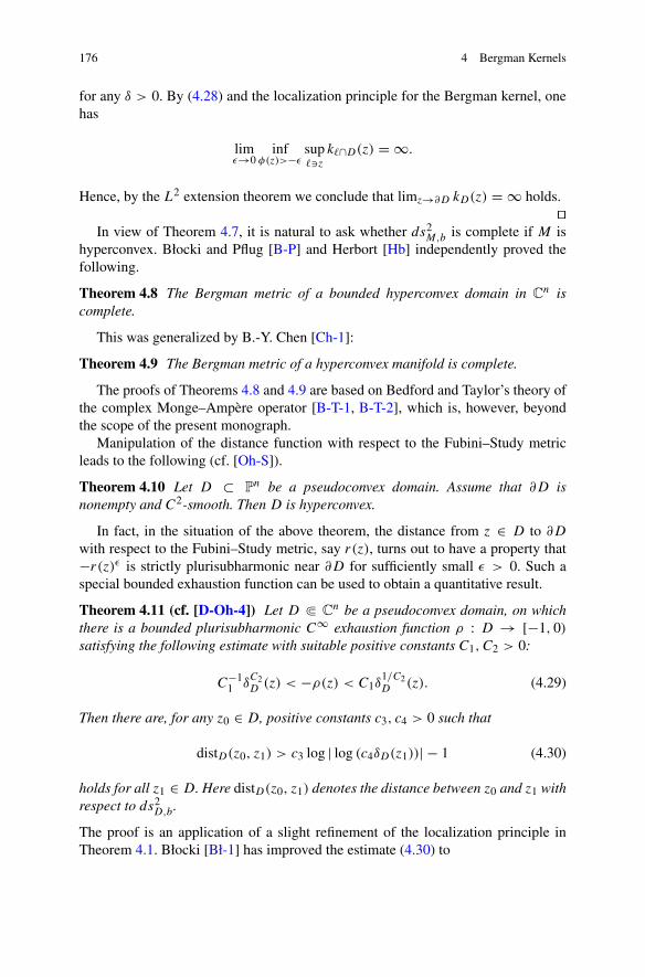
176 4 Bergman Kernels
for any δ > 0. By (4.28) and the localization principle for the Bergman kernel, onehas
limε→0
infφ(z)>−ε sup
��zk�∩D(z) = ∞.
Hence, by the L2 extension theorem we conclude that limz→∂D kD(z) = ∞ holds.��
In view of Theorem 4.7, it is natural to ask whether ds2M,b is complete if M is
hyperconvex. Błocki and Pflug [B-P] and Herbort [Hb] independently proved thefollowing.
Theorem 4.8 The Bergman metric of a bounded hyperconvex domain in Cn is
complete.
This was generalized by B.-Y. Chen [Ch-1]:
Theorem 4.9 The Bergman metric of a hyperconvex manifold is complete.
The proofs of Theorems 4.8 and 4.9 are based on Bedford and Taylor’s theory ofthe complex Monge–Ampère operator [B-T-1, B-T-2], which is, however, beyondthe scope of the present monograph.
Manipulation of the distance function with respect to the Fubini–Study metricleads to the following (cf. [Oh-S]).
Theorem 4.10 Let D ⊂ Pn be a pseudoconvex domain. Assume that ∂D is
nonempty and C2-smooth. Then D is hyperconvex.
In fact, in the situation of the above theorem, the distance from z ∈ D to ∂D
with respect to the Fubini–Study metric, say r(z), turns out to have a property that−r(z)ε is strictly plurisubharmonic near ∂D for sufficiently small ε > 0. Such aspecial bounded exhaustion function can be used to obtain a quantitative result.
Theorem 4.11 (cf. [D-Oh-4]) Let D � Cn be a pseudoconvex domain, on which
there is a bounded plurisubharmonic C∞ exhaustion function ρ : D → [−1, 0)satisfying the following estimate with suitable positive constants C1, C2 > 0:
C−11 δ
C2D (z) < −ρ(z) < C1δ
1/C2D (z). (4.29)
Then there are, for any z0 ∈ D, positive constants c3, c4 > 0 such that
distD(z0, z1) > c3 log | log (c4δD(z1))| − 1 (4.30)
holds for all z1 ∈ D. Here distD(z0, z1) denotes the distance between z0 and z1 withrespect to ds2
D,b.
The proof is an application of a slight refinement of the localization principle inTheorem 4.1. Błocki [Bł-1] has improved the estimate (4.30) to

4.2 The Boundary Behavior 177
distD(z0, z1) >log 1/δD(z1)
C log | log (c4δD(z1))| , C > 0. (4.31)
The proof relies on the pluripotential theory. Whether or not
distD(z0, z1) >log 1/δD(z1)
C, C > 0 (4.32)
holds remains an open question.
4.2.4 Comparison with a Capacity Function
Let D be a domain in C. Then, because of the transformation formula (4.9), kDis closely related to the theory of conformal mappings and related quantities suchas capacity functions (cf. [A, Ca, S-O] and [Su-2]). In view of the L2 methodin Chap. 2, it is easy to see that kD �≡ 0 if there exists a bounded nonconstantsubharmonic function on D, or equivalently, there exists a continuous functiong : D ×D→ [−∞, 0) such that the following hold for any w ∈ D:
(i) ∂∂g(∗, w) = 0 on D − {w}.(ii) g(z,w)− log |z− w| is bounded on a neighborhood of w.
The maximum element, say gD , of the set of such g is nothing but the Greenfunction of D. Accordingly, kD(z) �≡ 0 if the Green function exists on D.
We put
γ (z)(= γD(z)) = limw→z
(gD(z,w)− log |z− w|) (4.33)
and
cβ(z)(= cβ,D(z)) = eγ (z). (4.34)
γ and cβ are called the Robin function and the logarithmic capacity on D,respectively. It is straightforward that cβ(z) = (1−|z|2)−1 if D = D. Hence πkD =c2β .
Example 4.5 Let D(r) = {z ∈ C; |z| < r}. Then
gD(r)(z, w) = log∣∣∣ r(z− w)
r2 − wz
∣∣∣, (4.35)
γD(r)(z) = logr
r2 − |z|2 , (4.36)
cβ,D(r)(z) = r
r2 − |z|2 (4.37)

178 4 Bergman Kernels
and
kD(r)(z) = 1
π
r2
(r2 − |z|2)2 . (4.38)
Letting γ ≡ −∞ and cβ ≡ 0 if gD does not exist, one can say that kD ≡ 0if and only if cβ ≡ 0, as was observed by Oikawa and Sario in [S-O]. In fact, thiselementary but nontrivial remark is an interpretation of Carleson’s theorem on thenegligible singularities of Lp holomorphic functions (cf. [Ca, §VI. Theorem 1]).The main ingredient of [Ca] is a systematic study of “thin sets” by means of capaci-ties, Hausdorff measures, arithmetical conditions etc., dealing with the significanceof these concepts to existence problems for harmonic and holomorphic functions,boundary behavior, convergence of expansions and to harmonic analysis. Based onthis, Oikawa and Sario suggested comparing kD and cβ for any domain D. Thequestion makes sense for Riemann surfaces. Namely, using the local coordinates zand w in (4.33) and (4.34), we regard c2
β,M(z) dz⊗ dz as a section of T 1,0M ⊗ T
0,1M ,
so that the question is to compare KM(z) and c2β,M(z) dz⊗dz. By the way, the main
theme of [S-O] is the study of the boundary behavior of conformal mappings aimingat applications to the classification of open (= noncompact ) Riemann surfaces. Atthat time, a general question which attracted attention was the relation between thefunction spaces on a Riemann surface M and the magnitude of its boundary. Atypical approach was to consider an extremal problem in such a way that trivialityof the solution implies degeneration of certain function spaces (cf. [A-Bl]). KM andcβ,M are certainly solutions of extremal problems on M . In this context, Oikawa andSario also asked for comparison of KM with the Ahlfors constant
cB(z) := sup|f |≤1|f ′(z)|,
where f ∈ O(M). N. Suita (1933–2002) first considered this latter question andsolved it completely in [Su-1] with a sharp bound by generalizing Hejhal’s resultin [Hj’72] for smoothly bounded domains. After that, he proceeded to study therelation between KM and cβ .
As for the annuli Ar := {r < |z| < 1}, 0 ≤ r < 1, he proved the following in[Su-1].
Theorem 4.12 πkAr (z) ≥ c2β,Ar
(z) holds for all z ∈ Ar . The equality holds if andonly if r = 0.
Suita proved this by exploiting a formula of Zarankiewicz [Za] which expresseskAr in terms of the Weierstrass functions.
Suita’s conjecture. πKM(z) ≥ c2β,M(z) dz⊗dz holds for any Riemann surfaceM .
Moreover, the equality holds if and only if M is conformally (=biholomorphically)equivalent to D \ E for some E satisfying cβ,C\E ≡ 0.

4.2 The Boundary Behavior 179
In [Oh-16, Addendum], the L2 extension theorem was applied to Suita’sconjecture, and 750πKM ≥ c2
β,M was obtained for any Riemann surface M . In2012, Z. Błocki [Bł-2] proved:
Theorem 4.13 πkD ≥ c2β holds for any plane domain D.
Błocki’s proof is a refinement of a simplified variant of [Oh-T-1] by B.-Y. Chen[Ch-2]. For that, Błocki had to solve an ODE problem for two unknown functions.
The following sharpened version of Theorem 4.13 is in [Bł-3].
Theorem 4.14 Let D be a pseudoconvex domain in Cn and let
GD,w = sup {u ∈ PSH(D); u < 0 and lim supz→w
(u(z)− log |z− w|) <∞}.
Then
kD(w) ≥ 1
e2naVol ({GD,w < −a}) . (4.39)
Here Vol (·) denotes the Euclidean volume.
Proof Let G = GD,w and
χ(t) =⎧⎨⎩
0 t ≥ −a∫ −ta
s−1e−ns ds t < −a.
Then, solving the ∂-equation ∂α = ∂(χ ◦ G) with α ∈ L0,0(2) (D, e
−2nG) in such away that
∫D
|α|2 ≤ C Vol ({G < −a})
where C is an absolute constant, one has a holomorphic function f := χ ◦ G − α
satisfying
f (w) = χ(−∞) =∫ ∞na
s−1e−s ds =: E (na).
Since
‖f ‖ ≤ ‖χ ◦G‖ + ‖α‖ ≤ (χ(−∞)+√C)√Vol ({G < −a}),
the estimate
kD(w) ≥ |f (w)|2
‖f ‖2 ≥ c(n, a)
Vol ({G < −a})

180 4 Bergman Kernels
holds, where
c(n, a) = E (na)2
(E (na)+√C)2 .
For any m ∈ N, let D = Dm ⊂ Cnm and w = (w, . . . , w) ∈ D. Then k
D(w) =
(kD(w))m. Since G
D,w(z1, . . . , zm) = max1≤j≤m G(zj ), one has
Vol ({GD,w
< −a}) = Vol ({G < −a})m.
Hence, by the above estimate applied for D,
(kD(w))m ≥ c(nm, a)
(Vol ({G < −a}))m .
The desired inequality follows from the fact that
limm→∞ c(nm, a)1/m = e−2na. ��
In 2013, Q. Guan and X.-Y. Zhou [G-Z-1] proved the following, also byexploiting the solutions of an ODE problem.
Theorem 4.15 Suita’s conjecture is true for any Riemann surface.
Theorem 4.15 is a corollary of Theorem 3.4 except for the equality criterion.There exists an intimate relation between kD and gD besides the above inequal-
ity:
πkD(z,w) = 2∂2
∂z∂wgD(z,w) (Bergman–Schiffer formula) (4.40)
and
πkD(z) = ∂2
∂z∂zγD(z) (Suita’s formula) (4.41)
F. Maitani and H. Yamaguchi [M-Y] have exploited (4.40) to obtain an interestingvariational property of kD , which was generalized by Berndtsson [Brd’06] andeventually led Berndtsson and Lempert [Brd-L] to discover a completely new proofof Theorem 3.3. These materials will be discussed in Sects. 4.4.2, 4.4.3, 4.4.4 and4.4.5. According to Lempert, the final blow was inspired by Theorem 4.14.
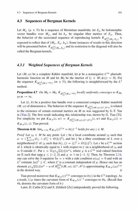
4.3 Sequences of Bergman Kernels 181
4.3 Sequences of Bergman Kernels
Let Mμ (μ ∈ N) be a sequence of Hermitian manifolds, let Eμ be holomorphicvector bundles over Mμ, and let hμ be singular fiber metrics of Eμ. Then,the behavior of the associated sequence of reproducing kernels K
H0,0(2) (Mμ,Eμ)
is
expected to reflect that of (Mμ,Eμ, hμ). Some instances of results in this directionwill be presented below. K
H0,0(2) (Mμ,Eμ)
and its restriction to the diagonal will also be
called the Bergman kernels.
4.3.1 Weighted Sequences of Bergman Kernels
Let (M,ω) be a complete Kähler manifold, let φ be a nonnegative C∞ plurisub-harmonic function on M and let M0 be the interior of {z ∈ M;φ(z) = 0}. Forthe sequence K
Hn,0(2) (M,e−mφ), (m ∈ N), the following is straightforward by the L2
method.
Proposition 4.7 On M0 ×M0, KHn,0(2) (M,e−mφ) locally uniformly converges to KM0
as m→∞.
Let (L, b) be a positive line bundle over a connected compact Kähler manifold(M,ω) of dimension n. The behavior of the sequence K
H0,0(2) ((M,ω),(Lμ,bμ))
is related
to the existence of certain extremal metrics on M as was suggested by S.-T. Yauin [Yau-2]. The first result indicating this relationship was shown by G. Tian [Ti].For simplicity we put KM,μ(z,w) = K
H0,0(2) ((M,ω),(Lμ,bμ))
(z, w) and KM,μ(z) =KM,μ(z, z). Tian proved:
Theorem 4.16 limμ→∞KM,μ(z)1/μ = b(z)−1 holds for any z ∈ M .
Proof Let z0 ∈ M be any point. Let z be a local coordinate around z0 such thatω = i
∑nj=1 dzj ∧ dzj + O(‖z‖2), and let ζ be a fiber coordinate of L over a
neighborhood U of z0 such that b(z, ζ ) = |ζ |2 + O(‖z‖2). Let s be a C∞ sectionof L which is identically equal to 1 with respect to ζ on a neighborhood of z0 and≡ 0 outside U . Put v = ∂(χ(
√μ‖z‖)sμ), where χ is a C∞ real-valued function
on R such that suppχ ⊂ [−2, 2] and χ ≡ 1 on [−1, 1]. Then, by Theorem 2.14,one can solve the ∂-equation ∂u = v with a side condition u(z0) = 0 and with anL2 estimate ‖u‖2 ≤ C, where C is a constant independent of μ. Hence one has anelement χ(
√μ‖z‖)sμ − u of H 0,0
(2) ((M,ω), (Lμ, bμ)) approximating KM,μ(z0)1/μ
in the desired way. ��Tian proved moreover that KM,μ(z)
1/μ converges to b(z) in the C2-topology. Asa result, 1/μ times the curvature form of KM,μ(z)
−1 converges to Θb. (Recall thatΘb denotes the curvature form of b.)
Later, D. Catlin [Ct] and S. Zelditch [Ze] independently proved the following.
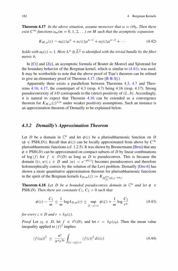
182 4 Bergman Kernels
Theorem 4.17 In the above situation, assume moreover that ω = iΘb. Then thereexist C∞ functions am(m = 0, 1, 2, . . .) on M such that the asymptotic expansion
KM,μ(z) ∼ a0(z)μn + a1(z)μ
n−1 + a2(z)μn−2 + · · · (4.42)
holds with a0(z) = 1. Here Lμ⊗Lμ is identified with the trivial bundle by the fibermetric b.
In [Ct] and [Ze], an asymptotic formula of Boutet de Monvel and Sjöstrand forthe boundary behavior of the Bergman kernel, which is similar to (4.41), was used.It may be worthwhile to note that the above proof of Tian’s theorem can be refinedto give an elementary proof of Theorem 4.17. (See [B-B-S].)
Apparently there exists a parallelism between Theorems 4.3, 4.7 and Theo-rems 4.16, 4.17, the counterpart of 4.3 (resp. 4.7) being 4.16 (resp. 4.17). Strongpseudoconvexity of ∂D corresponds to the (strict) positivity of (L, b). Accordingly,it is natural to expect that Theorem 4.16 can be extended as a convergencetheorem for KM,μ(z)
1/μ under weaker positivity assumptions. Such an instance isan approximation theorem of Demailly to be explained below.
4.3.2 Demailly’s Approximation Theorem
Let D be a domain in Cn and let φ(z) be a plurisubharmonic function on D
(φ ∈ PSH(D)). Recall that φ(z) can be locally approximated from above by C∞plurisubharmonic functions (cf. 1.2.5). It was shown by Bremermann [Brm] that anyφ ∈ PSH(D) can be approximated on compact subsets of D by linear combinationsof log |f | for f ∈ O(D) as long as D is pseudoconvex. This is because thedomain {(z, w); z ∈ D and |w| < e−φ(z)} becomes pseudoconvex and thereforeholomorphically convex by the solution of the Levi problem. Demailly [Dm-6] hasshown a more quantitative approximation theorem for plurisubharmonic functionsin the spirit of the Bergman kernels kD,m(z) := K
H0,0(2) (D,e
−mφ).
Theorem 4.18 Let D be a bounded pseudoconvex domain in Cn and let φ ∈
PSH(D). Then there are constants C1, C2 > 0 such that
φ(z)− C1
m≤ 1
mlog kD,m(z) ≤ sup
|ζ−z|<rφ(ζ )+ 1
mlog
C2
rn(4.43)
for every z ∈ D and r < δD(z).
Proof Let z0 ∈ D, let f ∈ O(D), and let r < δD(z0). Then the mean valueinequality applied to |f |2 implies
|f (z0)|2 ≤ n!πnr2n
∫‖z−z0‖<r
|f (z)|2 dλ(z) (4.44)
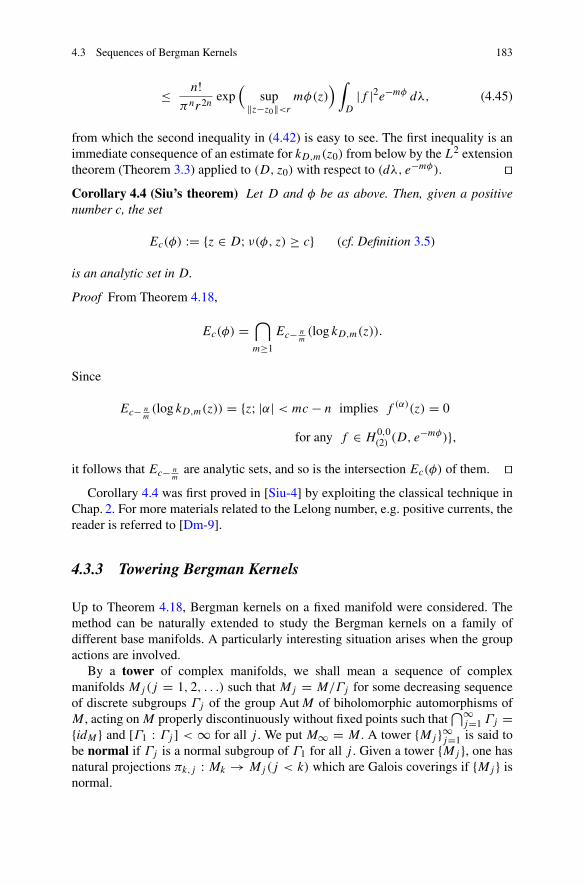
4.3 Sequences of Bergman Kernels 183
≤ n!πnr2n exp
(sup
‖z−z0‖<rmφ(z)
) ∫D
|f |2e−mφ dλ, (4.45)
from which the second inequality in (4.42) is easy to see. The first inequality is animmediate consequence of an estimate for kD,m(z0) from below by the L2 extensiontheorem (Theorem 3.3) applied to (D, z0) with respect to (dλ, e−mφ). ��Corollary 4.4 (Siu’s theorem) Let D and φ be as above. Then, given a positivenumber c, the set
Ec(φ) := {z ∈ D; ν(φ, z) ≥ c} (cf. Definition 3.5)
is an analytic set in D.
Proof From Theorem 4.18,
Ec(φ) =⋂m≥1
Ec− nm(log kD,m(z)).
Since
Ec− nm(log kD,m(z)) = {z; |α| < mc − n implies f (α)(z) = 0
for any f ∈ H 0,0(2) (D, e
−mφ)},
it follows that Ec− nm
are analytic sets, and so is the intersection Ec(φ) of them. ��Corollary 4.4 was first proved in [Siu-4] by exploiting the classical technique in
Chap. 2. For more materials related to the Lelong number, e.g. positive currents, thereader is referred to [Dm-9].
4.3.3 Towering Bergman Kernels
Up to Theorem 4.18, Bergman kernels on a fixed manifold were considered. Themethod can be naturally extended to study the Bergman kernels on a family ofdifferent base manifolds. A particularly interesting situation arises when the groupactions are involved.
By a tower of complex manifolds, we shall mean a sequence of complexmanifolds Mj(j = 1, 2, . . .) such that Mj = M/Γj for some decreasing sequenceof discrete subgroups Γj of the group AutM of biholomorphic automorphisms ofM , acting on M properly discontinuously without fixed points such that
⋂∞j=1 Γj ={idM} and [Γ1 : Γj ] < ∞ for all j . We put M∞ = M . A tower {Mj }∞j=1 is said to
be normal if Γj is a normal subgroup of Γ1 for all j . Given a tower {Mj }, one hasnatural projections πk,j : Mk → Mj(j < k) which are Galois coverings if {Mj } isnormal.
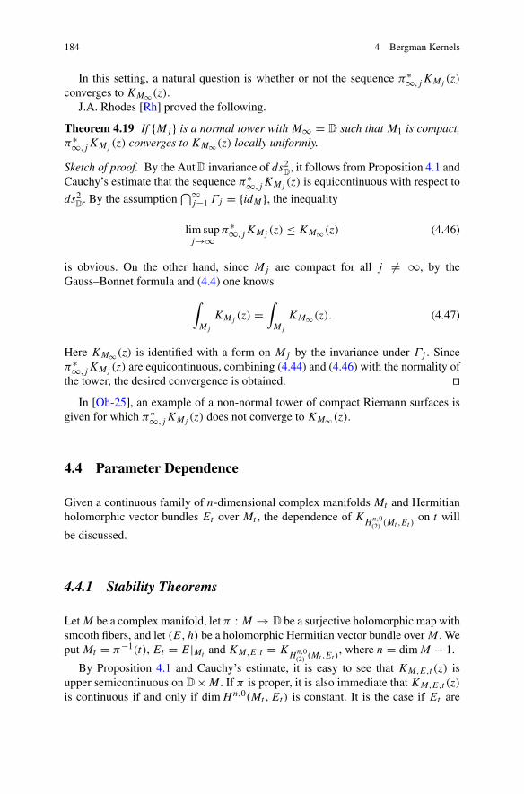
184 4 Bergman Kernels
In this setting, a natural question is whether or not the sequence π∗∞,jKMj(z)
converges to KM∞(z).J.A. Rhodes [Rh] proved the following.
Theorem 4.19 If {Mj } is a normal tower with M∞ = D such that M1 is compact,π∗∞,jKMj
(z) converges to KM∞(z) locally uniformly.
Sketch of proof. By the AutD invariance of ds2D
, it follows from Proposition 4.1 andCauchy’s estimate that the sequence π∗∞,jKMj
(z) is equicontinuous with respect to
ds2D
. By the assumption⋂∞
j=1 Γj = {idM}, the inequality
lim supj→∞
π∗∞,jKMj(z) ≤ KM∞(z) (4.46)
is obvious. On the other hand, since Mj are compact for all j �= ∞, by theGauss–Bonnet formula and (4.4) one knows
∫Mj
KMj(z) =
∫Mj
KM∞(z). (4.47)
Here KM∞(z) is identified with a form on Mj by the invariance under Γj . Sinceπ∗∞,jKMj
(z) are equicontinuous, combining (4.44) and (4.46) with the normality ofthe tower, the desired convergence is obtained. ��
In [Oh-25], an example of a non-normal tower of compact Riemann surfaces isgiven for which π∗∞,jKMj
(z) does not converge to KM∞(z).
4.4 Parameter Dependence
Given a continuous family of n-dimensional complex manifolds Mt and Hermitianholomorphic vector bundles Et over Mt , the dependence of K
Hn,0(2) (Mt ,Et )
on t will
be discussed.
4.4.1 Stability Theorems
LetM be a complex manifold, let π : M → D be a surjective holomorphic map withsmooth fibers, and let (E, h) be a holomorphic Hermitian vector bundle over M . Weput Mt = π−1(t), Et = E|Mt and KM,E,t = K
Hn,0(2) (Mt ,Et )
, where n = dimM − 1.
By Proposition 4.1 and Cauchy’s estimate, it is easy to see that KM,E,t (z) isupper semicontinuous on D×M . If π is proper, it is also immediate that KM,E,t (z)
is continuous if and only if dimHn,0(Mt , Et ) is constant. It is the case if Et are

4.4 Parameter Dependence 185
Nakano positive as is easily seen from Theorem 2.20. If Mt are Kählerian, thatdimHn,0(Mt) does not depend on t follows from the Hodge decomposition (cf.Theorem 2.33) and the upper semicontinuity of dimHp,q(Mt) in t . Moreover, aswe have noted in Sect. 3.1.4, the invariance of dimHn,0(Mt , Et ) is also true if M isholomorphically embeddable into some CP
N and Et ( KmMt
for some m ∈ N.For the case of Nakano positive bundles, one can also deduce from Theorem 2.14
a continuity result for nonproper π .
Theorem 4.20 Let π : M → D be a surjective holomorphic map with smoothfibers, and let (E, h) be a Nakano positive vector bundle over M . Assume that thereexists a complete Kähler metric on Mt for every t depending continuously on t andthere exists a Kähler metric ds2 on M and a constant c > 0 such that the leasteigenvalue of the curvature form of (E, h) with respect to ds2 is everywhere ≥ c.Then KM,E,t (z) is continuous.
Concerning the proof of Theorem 4.20, the reader is referred to [D-Oh-3] for theargument of solving the ∂-equation continuously in t by applying Theorem 2.14.
Remark 4.1 It might be interesting if one can find a natural condition for thecontinuity of KM,ωmMt
, where the fiber metric of KmMt
is induced from the Bergmankernel on Mt .
As for the Bergman metrics ds2Mt
, a criterion for the continuity can be describedsimilarly to that above.
Theorem 4.21 Let M,π, ds2t be as in Theorem 4.19. Assume moreover that there
exists a bounded strictly plurisubharmonic function on M . Then the family ofBergman metrics ds2
Mtis continuous on M × D.
Continuity of the derivatives of the Bergman kernels can be analyzed similarlyas long as the directions of derivatives are tangent to Mt (cf. [G-K]). As for thesmoothness with respect to t , not many facts seem to be known.
4.4.2 Maitani–Yamaguchi Theorem
F. Maitani and H. Yamaguchi [M-Y] observed from
log ke−φ(t)D(z) = − logπ + 2φ(t)+ 2∞∑j=1
(eφ(t)|z|)2jj
, (4.48)
which is known to hold for any upper semicontinuous function φ = φ(t) on D
by (4.38), that log ke−φ(t)D(z) is plurisubharmonic in (t, z) if and only if φ(t) issubharmonic in t , and generalized the result to Stein families of Riemann surfaces.As an exercise, let us verify by a straightforward computation that log ke−φ(t)D(z) isplurisubharmonic if φ(t) is subharmonic and in C2(D).
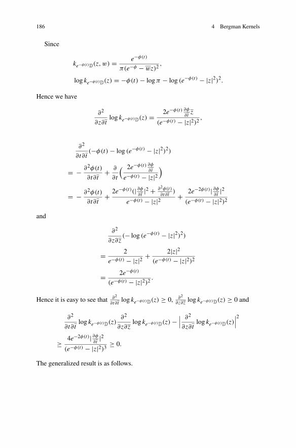
186 4 Bergman Kernels
Since
ke−φ(t)D(z, w) =e−φ(t)
π(e−φ − wz)2,
log ke−φ(t)D(z) = −φ(t)− logπ − log (e−φ(t) − |z|2)2.
Hence we have
∂2
∂z∂tlog ke−φ(t)D(z) =
2e−φ(t) ∂φ∂tz
(e−φ(t) − |z|2)2 ,
∂2
∂t∂t(−φ(t)− log (e−φ(t) − |z|2)2)
= − ∂2φ(t)
∂t∂t+ ∂
∂t
( 2e−φ(t) ∂φ∂t
e−φ(t) − |z|2)
= − ∂2φ(t)
∂t∂t+ 2e−φ(t)(| ∂φ
∂t|2 + ∂2φ(t)
∂t∂t)
e−φ(t) − |z|2 + 2e−2φ(t)| ∂φ∂t|2
(e−φ(t) − |z|2)2
and
∂2
∂z∂z(− log (e−φ(t) − |z|2)2)
= 2
e−φ(t) − |z|2 +2|z|2
(e−φ(t) − |z|2)2
= 2e−φ(t)
(e−φ(t) − |z|2)2 .
Hence it is easy to see that ∂2
∂t∂tlog ke−φ(t)D(z) ≥ 0, ∂2
∂z∂zlog ke−φ(t)D(z) ≥ 0 and
∂2
∂t∂tlog ke−φ(t)D(z)
∂2
∂z∂zlog ke−φ(t)D(z)−
∣∣∣ ∂2
∂z∂tlog ke−φ(t)D(z)
∣∣∣2
≥ 4e−2φ(t)| ∂φ∂t|2
(e−φ(t) − |z|2)3 ≥ 0.
The generalized result is as follows.

4.4 Parameter Dependence 187
Theorem 4.22 Let p : D → D × C be a Riemann domain, let p1 : D × C → D
be the projection to the first factor, and let Dt = p−1({t} × C). Assume that D ispseudoconvex. Then log kDt
(z) (z ∈ Dt ) is plurisubharmonic on D .
Let us present below only a sketchy account on the proof of Theorem 4.22, sincethe result was further generalized by Berndtsson [Brd’06, Brd] and Guan and Zhou[G-Z-1] by completely different methods. Their proofs will be discussed later indetail.
Sketch of proof Since the assertion is local in t , one may assume that ∂D is smoothand Dt are domains with real analytic smooth boundary. Let Φ be a definingfunction of ∂D . We put g(t, z, w) = gDt
(z, w) and γ (t, z) = γDt(z).
Since
g(t, z, w) = log |z− w| + γ (t, z)+ h(t, z, w), (4.49)
where h is harmonic in z in a neighborhood of w ∈ Dt and h(t, w,w) = 0 forall t , ∂γ (t, z)/∂t and ∂2γ (t, z)/∂t∂t are harmonic on Dt . Hence, by a generalizedPoisson formula on Dt , one obtains
∂γ (t, w)
∂t= 1
π
∫∂Dt
(∂Φ∂t
/∣∣∣∂Φ∂z
∣∣∣)∣∣∣∂g(t, z, w)
∂z
∣∣∣2 ds (4.50)
Here ds denotes the arc length element of ∂Dt . Similarly, modifying the contourintegral by Stokes’ formula, one has
∂2γ (t, w)
∂t∂t= 1
π
∫∂Dt
L(t, z)
∣∣∣∂g(t, z, w)∂z
∣∣∣2 ds + 4
π
∫Dt
∣∣∣∂2g(t, z, w)
∂t∂z
∣∣∣2 dλ,(4.51)
where
L(t, z) =(∂2Φ
∂t∂t
∣∣∣∂Φ∂z
∣∣∣2 − 2Re{ ∂2Φ
∂t∂z
∂Φ
∂t
∂Φ
∂z
}+∣∣∣∂Φ∂t
∣∣∣2 ∂2Φ
∂z∂z
)/∣∣∣∂Φ∂z
∣∣∣3.(4.52)
Let
L (t, z, w) = 2
π
∂g(t, z, w)
∂z∂w
and
K (t, z, w) = 2
π
∂g(t, z, w)
∂z∂w.
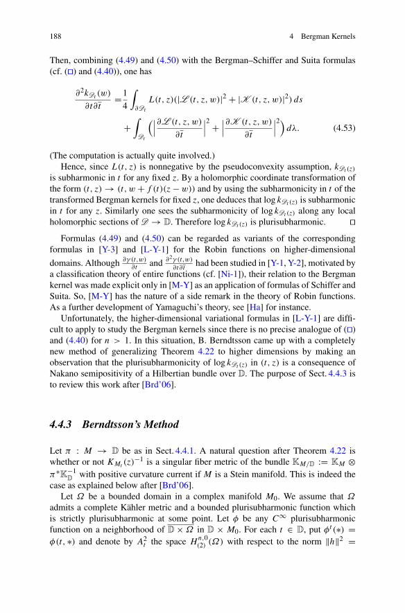
188 4 Bergman Kernels
Then, combining (4.49) and (4.50) with the Bergman–Schiffer and Suita formulas(cf. (��) and (4.40)), one has
∂2kDt(w)
∂t∂t=1
4
∫∂Dt
L(t, z)(|L (t, z, w)|2 + |K (t, z, w)|2) ds
+∫
Dt
(∣∣∣∂L (t, z, w)
∂t
∣∣∣2 +∣∣∣∂K (t, z, w)
∂t
∣∣∣2)dλ. (4.53)
(The computation is actually quite involved.)Hence, since L(t, z) is nonnegative by the pseudoconvexity assumption, kDt (z)
is subharmonic in t for any fixed z. By a holomorphic coordinate transformation ofthe form (t, z)→ (t, w+ f (t)(z−w)) and by using the subharmonicity in t of thetransformed Bergman kernels for fixed z, one deduces that log kDt (z) is subharmonicin t for any z. Similarly one sees the subharmonicity of log kDt (z) along any localholomorphic sections of D → D. Therefore log kDt (z) is plurisubharmonic. ��
Formulas (4.49) and (4.50) can be regarded as variants of the correspondingformulas in [Y-3] and [L-Y-1] for the Robin functions on higher-dimensional
domains. Although ∂γ (t,w)∂t
and ∂2γ (t,w)
∂t∂thad been studied in [Y-1, Y-2], motivated by
a classification theory of entire functions (cf. [Ni-1]), their relation to the Bergmankernel was made explicit only in [M-Y] as an application of formulas of Schiffer andSuita. So, [M-Y] has the nature of a side remark in the theory of Robin functions.As a further development of Yamaguchi’s theory, see [Ha] for instance.
Unfortunately, the higher-dimensional variational formulas in [L-Y-1] are diffi-cult to apply to study the Bergman kernels since there is no precise analogue of (��)and (4.40) for n > 1. In this situation, B. Berndtsson came up with a completelynew method of generalizing Theorem 4.22 to higher dimensions by making anobservation that the plurisubharmonicity of log kDt (z) in (t, z) is a consequence ofNakano semipositivity of a Hilbertian bundle over D. The purpose of Sect. 4.4.3 isto review this work after [Brd’06].
4.4.3 Berndtsson’s Method
Let π : M → D be as in Sect. 4.4.1. A natural question after Theorem 4.22 iswhether or not KMt (z)
−1 is a singular fiber metric of the bundle KM/D := KM ⊗π∗K−1
Dwith positive curvature current if M is a Stein manifold. This is indeed the
case as explained below after [Brd’06].Let Ω be a bounded domain in a complex manifold M0. We assume that Ω
admits a complete Kähler metric and a bounded plurisubharmonic function whichis strictly plurisubharmonic at some point. Let φ be any C∞ plurisubharmonicfunction on a neighborhood of D×Ω in D × M0. For each t ∈ D, put φt (∗) =φ(t, ∗) and denote by A2
t the space Hn,0(2) (Ω) with respect to the norm ‖h‖2 =
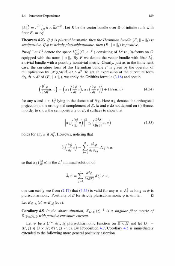
4.4 Parameter Dependence 189
‖h‖2t = in2 ∫
Ωh ∧ he−φt . Let E be the vector bundle over D of infinite rank with
fiber Et = A2t .
Theorem 4.23 If φ is plurisubharmonic, then the Hermitian bundle (E, ‖ ∗ ‖t ) issemipositive. If φ is strictly plurisubharmonic, then (E, ‖ ∗ ‖t ) is positive.
Proof Let L2t denote the space Ln,0(2) (Ω, e−φt ) consisting of L2 (n, 0)-forms on Ω
equipped with the norm ‖ ∗ ‖t . By F we denote the vector bundle with fiber L2t ,
a trivial bundle with a possibly nontrivial metric. Clearly, just as in the finite rankcase, the curvature form of this Hermitian bundle F is given by the operator ofmultiplication by (∂2φ/∂t∂t) dt ∧ dt . To get an expression of the curvature formΘE dt ∧ dt of (E, ‖ ∗ ‖t ), we apply the Griffiths formula (3.16) and obtain
( ∂2φ
∂t∂tu, v)=(π⊥(∂φ∂tu), π⊥
(∂φ∂tv))+ (ΘEu, v) (4.54)
for any u and v ∈ L2t lying in the domain of ΘE . Here π⊥ denotes the orthogonal
projection to the orthogonal complement of E. (u and v do not depend on t .) Hence,in order to show the semipositivity of E, it suffices to show that
∥∥∥π⊥(∂φ∂tu)∥∥∥2 ≤
( ∂2φ
∂t∂tu, u
)(4.55)
holds for any u ∈ A2t . However, noticing that
∂z
(∂φ∂tu)=
n∑j=1
∂2φ
∂t∂zjdzj ∧ u,
so that π⊥( ∂φ∂t u) is the L2 minimal solution of
∂zw =n∑
j=1
∂2φ
∂t∂zjdzj ∧ u,
one can easily see from (2.17) that (4.55) is valid for any u ∈ A2t as long as φ is
plurisubharmonic. Positivity of E for strictly plurisubharmonic φ is similar. ��Let KΩ,φt (z) = KA2
t(z, z).
Corollary 4.5 In the above situation, KΩ,φt (z)−1 is a singular fiber metric of
K(D×Ω)/D with positive curvature current.
Let ψ be a C∞ strictly plurisubharmonic function on D×Ω and let Dc ={(t, z) ∈ D × Ω;ψ(t, z) < c}. By Proposition 4.7, Corollary 4.5 is immediatelyextended to the following more general positivity assertion.
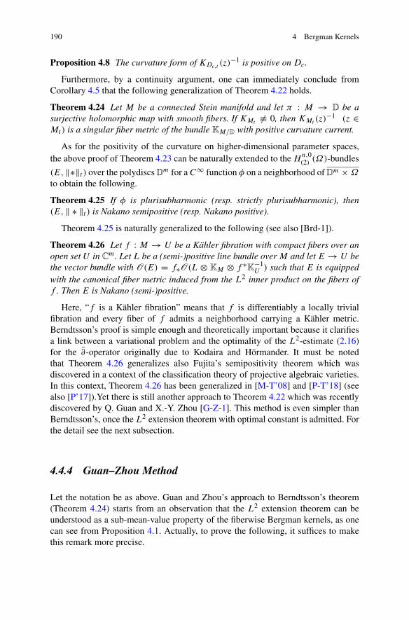
190 4 Bergman Kernels
Proposition 4.8 The curvature form of KDc,t (z)−1 is positive on Dc.
Furthermore, by a continuity argument, one can immediately conclude fromCorollary 4.5 that the following generalization of Theorem 4.22 holds.
Theorem 4.24 Let M be a connected Stein manifold and let π : M → D be asurjective holomorphic map with smooth fibers. If KMt �≡ 0, then KMt (z)
−1 (z ∈Mt) is a singular fiber metric of the bundle KM/D with positive curvature current.
As for the positivity of the curvature on higher-dimensional parameter spaces,the above proof of Theorem 4.23 can be naturally extended to the Hn,0
(2) (Ω)-bundles
(E, ‖∗‖t ) over the polydiscs Dm for aC∞ function φ on a neighborhood of Dm ×Ω
to obtain the following.
Theorem 4.25 If φ is plurisubharmonic (resp. strictly plurisubharmonic), then(E, ‖ ∗ ‖t ) is Nakano semipositive (resp. Nakano positive).
Theorem 4.25 is naturally generalized to the following (see also [Brd-1]).
Theorem 4.26 Let f : M → U be a Kähler fibration with compact fibers over anopen set U in C
m. Let L be a (semi-)positive line bundle over M and let E→ U bethe vector bundle with O(E) = f∗O(L ⊗ KM ⊗ f ∗K−1
U ) such that E is equippedwith the canonical fiber metric induced from the L2 inner product on the fibers off . Then E is Nakano (semi-)positive.
Here, “f is a Kähler fibration” means that f is differentiably a locally trivialfibration and every fiber of f admits a neighborhood carrying a Kähler metric.Berndtsson’s proof is simple enough and theoretically important because it clarifiesa link between a variational problem and the optimality of the L2-estimate (2.16)for the ∂-operator originally due to Kodaira and Hörmander. It must be notedthat Theorem 4.26 generalizes also Fujita’s semipositivity theorem which wasdiscovered in a context of the classification theory of projective algebraic varieties.In this context, Theorem 4.26 has been generalized in [M-T’08] and [P-T’18] (seealso [P’17]).Yet there is still another approach to Theorem 4.22 which was recentlydiscovered by Q. Guan and X.-Y. Zhou [G-Z-1]. This method is even simpler thanBerndtsson’s, once the L2 extension theorem with optimal constant is admitted. Forthe detail see the next subsection.
4.4.4 Guan–Zhou Method
Let the notation be as above. Guan and Zhou’s approach to Berndtsson’s theorem(Theorem 4.24) starts from an observation that the L2 extension theorem can beunderstood as a sub-mean-value property of the fiberwise Bergman kernels, as onecan see from Proposition 4.1. Actually, to prove the following, it suffices to makethis remark more precise.
4.4 Parameter Dependence 191
Theorem 4.27 (cf. [G-Z-1]) Let M be a connected complex manifold and let p :M → D be a holomorphic map with smooth fibers. Assume that there exists ananalytic set X ⊂ M such that M \ X is Stein and p−1(0) ∩ X is nowhere densein p−1(0). Then, either KMt (z) ≡ 0 or KMt (z)
−1 is a singular fiber metric of thebundle KM/D with positive curvature current.
Proof By Theorem 1.8 it suffices to prove the assertion by assuming that X = ∅.Let z0 be any point of M0 and let (t, z) be a local coordinate of M around (0, z0).In terms of (t, z), the Bergman kernels KMt (z) are expressed as
KMt (z) = 2−nk(t, z) dz1 ∧ dz2 ∧ · · · ∧ dzn ⊗ dz1 ∧ dz2 ∧ · · · ∧ dzn. (4.56)
To prove the assertion, it suffices to show that the average of log k(t, z0) over |t | < r
is ≥ log k(0, z0) for such a coordinate (t, z). For that, let us put
u0 = KM0(z, z0)√k(0, z0) dz1 ∧ dz2 ∧ · · · ∧ dzn . (4.57)
By the L2 extension theorem, if 0 < r ≤ 1 there exists a holomorphic section ur ofωM/D|p−1({|t |<r}) such that
u0 = ur |M0 and ‖ur‖2 ≤ πr2. (4.58)
On the other hand, by Proposition 4.1,
KMt (z) ≥ur (z)⊗ ur (z)
‖ur‖2t(4.59)
if |t | < r . Here the right-hand side is to be read as 0 if ‖ur‖t = ∞. Note that thelatter part of (4.57) means
1 ≥ 1
πr2
∫|t |<r‖ur‖2t dλt . (4.60)
Hence, in view of (4.55) and (4.58) with z = z0, (4.59) implies
1 ≥ exp1
πr2
∫|t |<r
(2 log |ur (t, z0)/(dz1 ∧ dz2 ∧ · · · ∧ dzn)| − log k(t, z0)) dλt
(4.61)
by the convexity of the function y = ex . But log |ur (t, z0)/(dz1 ∧ dz2 ∧ · · · ∧ dzn)|is harmonic, so that, in view of (4.56) and the first half of (4.57), the desired sub-mean-value property

192 4 Bergman Kernels
log k(0, z0) ≤ 1
πr2
∫|t |<r
log k(t, z0) dλt (4.62)
follows from (4.60). ��Theorems 3.3 and 3.4 can be deduced from Theorem 4.26 by generalizing the aboveargument. See [Brd-L] for the detail. An expository but sketchy account will begiven in the next subsection.
4.4.5 Berndtsson–Lempert Theory and Beyond
In 2014, Berndtsson and Lempert [Brd-L] found a remarkable connection betweenthe plurisubharmonicity of log kD and Theorem 3.3. To illustrate the idea of [Brd-L],let us begin with an alternate proof of Theorem 3.2 along with Lempert’s proof ofTheorem 4.13 which was presented in [Bł’15, Introduction].
Proof of Theorem 3.2 It suffices to show that πkD(0) ≥ 1, or equivalently thatlog(πkD(0)) ≥ 0. By the Maitani–Yamaguchi theorem (Theorem 4.22), log k|t |D(0)is subharmonic in log t . Since log k|t |D(0) depends only on log |t |, it is convex inlog |t |. Therefore, the function
− logπkD(0)+ logπk|t |D(0)+ log |t |2
turns out to be increasing in log |t |, since it is convex and bounded. Hence
limt→0
(− logπkD(0)+ logπk|t |D(0)+ log |t |2)
≤ limt→1
(− logπkD(0)+ logπk|t |D(0)+ log |t |2) = 0.
Admitting that Theorem 3.2 is infinitesimally true, i.e. that limt→0 πk|t |D(0)|t |2 =1, we obtain the desired conclusion. ��
Keeping this argument in mind, it may not be too hard to generalize it to proveTheorem 3.26 for any pseudoconvex domain Ω ⊂ C
n−1 × D ⊂ Cn. Namely, it
suffices to consider the domain {(z, t) ∈ Ω × D; |zn| < egD(t,0)} and apply (alimiting case of) Theorem 4.23 to the projection to the last factor. More detailedargument is as follows.
Proof of Theorem 3.26. Let A2ϕ(Ω) (resp. A2
ϕ(Ω′)) denote the space of holomor-
phic functions on Ω (resp. on Ω ′) with respect to the Lebesgue measure. To provethe assertion, it suffices to show that
supf∈A2
ϕ(Ω′),‖f ‖=1
inf {‖F‖2 | F ∈ A2ϕ(Ω), F |Ω ′ = f } ≤ πcD(0)
−2.

4.4 Parameter Dependence 193
For that we look at the function
supf∈A2
ϕ(Ω′),‖f ‖=1
inf {‖F‖2 | F ∈ A2ϕ(Ωt ), F |Ω ′ = f },
where Ωt = {z ∈ Ω | |z1| < egD(t,0)}. Since the counterpart oflimt→0 πk|t |D(0)|t |2 = 1 in the above argument is obviously true from the definitionof cD(t), it suffices to show that this function is decreasing as a function of gD(t, 0).To evaluate the magnitude of inf {‖F‖2 | F ∈ A2
ϕ(Ωt ), F |Ω ′ = f } we exploit theorthogonal decomposition
A2ϕ(Ωt ) = A2
ϕ(Ω′)⊕ (A2
ϕ(Ωt ) ∩I (Ωt )),
where I (Ωt ) denotes the subspace of O(Ωt ) consisting of the functions vanishingon Ω ′ and the norm in A2
ϕ(Ω′) on the right hand side is that of the quotient
A2ϕ(Ωt )/(A
2ϕ(Ωt ) ∩I (Ωt )), i.e.
‖f ‖2t := minF∈A2
ϕ(Ωt ), F |Ω′=f‖F‖2.
In this situation, the proof will be over if the function gG(t, 0) �→ ‖f ‖t e−gD(t,0)turns out to be decreasing for every f ∈ A2
ϕ(Ω′) \ {0}, because it will then follow
that
inf {‖F‖2 | F ∈ A2ϕ(Ω), F |Ω ′ = f } = lim
t→1‖f ‖2t e−2gD(t,0)
≤ limt→0‖f ‖2t e−2gD(t,0) = πcD(0)
−2‖f ‖.
To evaluate ‖f ‖t e−gD(t,0) we apply the equality
‖f ‖t = supξ∈A2
ϕ(Ω′)∗|ξ(f )|/‖ξ(t)‖,
where ‖ · ‖(t) denotes the dual norm of ‖ · ‖t . Since the monotonicity of functionsis preserved by taking the supremum, it suffices to show that ‖ξ‖(t)egD(t,0) isincreasing for every ξ �= 0. But this follows similarly to the above proof ofπkD(0) ≥ 1 from the subharmonicity of log ‖ξ‖(t), which is guaranteed byTheorem 4.23. ��
By this argument, an L2 extension theorem was proved in [Brd-L] for anypseudoconvex domain D ⊂ C
n, for any φ ∈ PSH(D) and for any complexsubmanifold V ⊂ D of codimension k with respect to
A2(D) ={f ∈ O(D);
∫D
|f |2e−φ <∞}
194 4 Bergman Kernels
and
A2(D) ={f ∈ O(V );
∫V
|f |2e−φ <∞}.
Here the integration is with respect to the Lebesgue measure and the volume elementon V induced by the euclidean metric, respectively. Let dV (z) be the distance fromz to V and let G be a negative plurisubharmonic function on D which satisfies
G(z) ≤ log d2V (z)+ A
and
G(z) ≥ log d2V (z)− B(z)
as z goes to V . Here A is some constant and B is a continuous function on D. Thenthe precise estimate of Berndtsson–Lempert is the following.
Theorem 4.28 Let f ∈ A2(V ). Then there is a function F in A2(D) whoserestriction to V euqals f , which satisfies
∫D
|F |2e−φ ≤ σk
∫V
|f |2e−φ+kB,
where σk is the volume of the unit ball in Ck .
It is easy to see that Theorem 3.26 is a corollary of Theorem 4.28. It turned outrecently that the method of Berndtsson and Lempert can be applied to prove an L2
extension theorem for jets of holomorphic functions (cf. [H’17-1] and [M-V’17]).Hosono [H’17-2] also obtained the following highly nontrivial refinement ofTheorem 3.2 by this method.
Theorem 4.29 In the above situation, assume that n = 1 and φ(0) = 0. LetD = {(z, w) ∈ C
2; z ∈ D, |w|2 < e−φ(z)} and assume that there exists a negativeplurisubharmonic function G on D satisfying log |z|2 + A(z,w) ≥ G ≥ log |z|2 −B(z,w) for some continuous functions A and B. Then there exists f ∈ O(D) suchthat f (0) = 1 and
∫D
|f (z)|2e−φ(z) dλz ≤∫D
eB(0,w) dλw.
4.5 Notes and Remarks
Since the Bergman kernel has many aspects of independent interest, some of themthat have not been mentioned above will be reviewed below.
4.5 Notes and Remarks 195
The transformation formula (4.8) for the Bergman kernel can be used to explorethe properties of biholomorphic maps. For instance, given a simply connecteddomain D � C and p ∈ D, the biholomorphic map f : D→ D with f (p) = 0 andf ′(p) > 0 can be expressed in terms of kD by using
kD(z, F (z))F ′(w) = f ′(z)kD(f (z), w) = f ′(z) 1
π(1− wf (z))2, (4.63)
where F = f−1. Indeed, by letting w = 0 one has
kD(z, p)F ′(0) = π−1f ′(z), (4.64)
which immediately yields a well-known formula
f (z) =√
π
kD(p, p)
∫ z
p
kD(ζ, p) dζ .
On the other hand, by differentiating (4.64) with respect to w one has
k′D(z, F (w))F ′(w)2 + kD(z, F (w))F ′′(w) = 2f ′(z)f (z) 1
π(1− wf (z))3,
(4.65)
where k′D(z,w) = ∂∂wkD(z,w). Letting w = 0 in (4.65) one has
k′D(z, p)F ′(0)2 + kD(z, p)F ′′(0) = 2π−1f ′(z)f (z). (4.66)
Dividing (4.66) by (4.64) one has
2F(z) = c1k′D(z, p)kD(z, p)
+ c2,
where c1 = F ′(0) and c2 = F ′′(0)/F ′(0). This shows that the mapping
k′D(z, p)kD(z, p)
is a biholomorphic map onto a disc.For multiply connected domains in C, Suita and Yamada [S-Y’76] showed that
the Bergman kernel must vanish at some point, so that the above expression losessome utility. On the other hand, for any bounded domain Ω in C
n, there is a
generalization ofk′D(z,p)kD(z,p)
which has significance as a global canonical coordinatein some cases. An explicit expression of this coordinate will be described below.
196 4 Bergman Kernels
Let
ds2Ω,b =
∑j,k
gj,k dzj ⊗ dzk
and let gkj be the (k, j)-th entry of the inverse matrix of (gjk). Then, for any p ∈ Ω ,we put
repp(z) = (ζ1(z), . . . , ζn(z)),
where
ζj (z) =∑k
gkj (p)(∂ log kΩ(z,w)
∂wk
− ∂ log kΩ(w,w)
∂wk
)∣∣∣w=p
.
Since ∂ζk∂z�|z=p = δ�k , the map repp is a holomorphic local coordinate around p.
Bergman has found the following.
Theorem 4.30 (cf. [B’50]) If f : Ω → Ω is a biholomorphic mapping of boundeddomains, the composite repf (p) ◦ f ◦ rep−1
p is C-linear.
The proof of Bergman is a direct computation using (4.8). Recently it wasobserved by S. Yoo [Y’16] that Theorem 4.28 is essentially a consequence of anobvious fact that the Bergman metric has locally a potential whose Taylor expansionhas no holomorohic or anti-holomorphic part.
It is well-known that the idea of linearizing biholomorphic maps was carriedover by Webster [W’79-1] and Bell [B’79], and culminated in [B-L’80] and [L’81]as the great simplification of the proof of Fefferman’s theorem for the C∞-smoothextendability of biholomorphic maps between C∞ strongly pseudoconvex domains.
The map k′D/kD is related to Suita’s conjecture in an intriguing manner. Let usfollow this passage for a while starting from
Theorem 4.31 (cf. [B’06, Theorem 2.2]) Let D1 and D2 be n-connected boundeddomains in C, each bounded by n non-intersectingC∞ smooth simple closed curves,and let f : D1 → D2 be a biholomorphic map. Given pj ∈ ∂Dj for j = 1, 2, there
exist aj1 and aj2 in Dj such that kDj(z, a
j
1 )/kDj(z, a
j
0 ) map the points of ∂Dj nearpj to smooth real-algebraic sets, and f becomes linear after these transformations.
The same procedure as in Theorem 4.29 can be carried out for Riemann surfaces.If Ω is a smoothly bounded domain in a compact Riemann surface M with an anti-holomorphic involution ι such that ∂Ω = {x ∈ M; ι(x) = x} (M is the doubleof Ω), it is known that the Bergman kernel KΩ extends to M meromorphically.More explicitly, letting fp : M → C be an n-to-one holomorphic map such thatfp(p) = 0 and fp(∂Ω) = ∂D, which exists and unique up to multiplication byeiθ ∈ ∂D, it is shown in [B’99] that the function

4.5 Notes and Remarks 197
fp(z)KΩ(z,w)fp(w)
dfp(z)⊗ dfp(w)
extends as a single-valued function to M ×M which is meromorphic in w and anti-meromorphic in z. In this situation, it was pointed out by Yamada [Y’98] that thevalidity of Suita’s conjecture implies that the function L(z,w) := L (0, z, w) forΩ = D0 in 4.4.2 is zero-free if M �= C. L(z,w) is known as the adjoint L-kernelof Ω , which is characterized, among the class of meromorphic function on Ω withthe same singularity as L(z,w) and with finite values
limε→0
∫Ω\{|z−w|<ε}
L(z,w)ω ∧ ω
for any ω(= ω(z)) ∈ H 1,0(2) (Ω), by the property that
limε→0
∫Ω\{|z−w|<ε}
L(z,w)ω ∧ ω = 0
holds for all ω ∈ H 1,0(2) (Ω) (see [S’97]).
The localization principle is the key idea in the proof of Theorem 4.3, as Hörman-der remarks in [Hö-3]. Theorem 4.4 is a far-reaching refinement of Theorem 4.3,involving the idea that geometric invariants of ∂D can be differentiated out fromthe coefficients φ(z) and ψ(z) in (4.25). Equation (4.24) says that the principalterm of the singularity of kD(z) at z0 is n!π−n�(z0)δD(z)
−n−1. For a class ofweakly pseudoconvex domains, the boundary behavior of kD(z) has been analyzedin the same spirit (cf. [H’83, D-H’93, D-H’94, B-S-Y’95, K’04, Ch-K-Oh’04]). Anillustrative result is in [H’83], where the Bergman kernel of the domain
Ω = {z ∈ C3;Re z1 + |z2|6 + |z2|2|z3|2 + |z3|6 < 0}
satisfies
−c1
δ3Ω log δΩ
< kΩ <−c2
δ3Ω log δΩ
on the set {(t, 0, 0); t < 0} near the origin for some positive constants c1 and c2.It follows from a direct generalization of the localization principle that, if ∂D is
spherical (= locally CR diffeomorphi to ∂Bn(0, 1)), then ψ vanishes to the infiniteorder along ∂D. The Ramadanov conjecture in [R’81] asserts conversely that thecondition ψ(z) = O(ρ∞) as z→ ∂D implies that ∂D is spherical. The conjecturewas proved for domains in C
2 by Graham and Burns [G’87]1 and Boutet de Monvel
1Graham [G’87] is based on an unpublished note of Burns. In [H-K-N’93] a computation neededin Graham’s proof is written.

198 4 Bergman Kernels
[BM’88] (see also [W’79-2]). The conditionψ = O(ρ∞) is satisfied if the Bergmanmetric is Kähler–Einstein (cf. [F-W’97]), so that combining a theorem of Lu Qi-Keng [L’66], asserting that a bounded domain with complete Bergman metric ofconstant holomorphic sectional curvature is biholomorphic to the ball, with Chengand Yau’s theorem on the uniqueness of complete Kähler–Einstein metrics (up toconstant) (cf. [C-Y’80]), one knows that the Ramadanov conjecture implies that Dis biholomorphic to the ball if and only if the Bergman metric is Kähler–Einstein.The latter is known as Cheng’s conjecture (cf. [F-W’97]).
Recently, it turned out that the Ramadanov conjecture is true if D is sufficientlyclose to the ball. Curry and Ebenfelt proved it for the case n = 3 and Hirachi provedit for the general case (cf. [C-E’18]).
An effective version of Theorem 4.9 was obtained in [Ch’17] by restrictinga class of hyperconvex domains. Let D ⊂ C
n be a domain with a negativeplurisubharmonic exhaustion function ρ. If −ρ(z) ≤ CδD(z)
α for some constantsα,C > 0, let α(D) be the supremum of such α. If there exists η > 0 such thatC−1δ
ηD < −ρ ≤ Cδ
ηD for some C > 0, let η(D) be the supremum of such η.
α(D) and η(D) are called the hyperconvexity index and the Diederich–Fornaessindex, respectively (cf. [D-F-1, A-B, F-S’16, H’08, H’17]). It is known that, ifD is a bounded psuedoconvex domain in C
n with Lipschitz boundary, then D ishyperconvex (cf. [Dem’87]) and η(D) > 0 (cf. [H’08, H’17]).
Theorem 4.32 (cf. [Ch’17, Theorem 1.7]) Let D ⊂ Cn be a bounded hyperconvex
domain with α(D) > 0. Then, for every 0 < r < 1 there exists a constant C > 0such that
|kD(z,w)|2kD(z)kD(w)
≤ C(
min{ ν(z)μ(z)
,ν(z)
μ(z)
})r, z, w ∈ D,
where μ = |ρ|/(1+ | log (−ρ)|) and ν = |ρ|(1+ | log (−ρ)|)n.
Combining Theorem 4.30 with an estimate of the form
1−√|kD(z,w)|2kD(z)kD(w)
≤ 2(distD(z,w))2,
the following generalization of (4.31) has been obtained.
Theorem 4.33 ([Ch’17, Corollary 1.8]) If D is a bounded hyperconvex domainwith α(D) > 0, there exists for any point z0 ∈ D a constant C > 0 such that
distD(z0, z) ≥ C| log δD(z)|
log | log δD(z)|holds for any z sufficiently close to ∂D.

4.5 Notes and Remarks 199
Concerning Theorem 4.17, see [M-M’07] for an extensive account coupled withDemailly’s complex Morse inequality and studies on the asymptotics of the analytictorsion.
In the case where the curvature form of (L, h) degenerates at a point z0 ∈ M , anexpansion of the form
limμ→∞
∣∣∣KM,μ(z)− μβ(a0 + a1
μα+ · · · + aN
μNα
)∣∣∣ = 0
was shown for some α, β > 0 under some homogeneity condition on h near z0 (cf.[Ch-K-N’11]).
Demailly [Dm-6] applied Theorem 4.18 to extend the definition of a positiveclosed current (i∂∂u)k , which was originally defined in Bedford–Taylor theory[B-T-1, B-T-2] for a bounded plurisubharmonic function u recursively as
(∂∂u)k = ∂∂(u(∂∂u)k−1).
For instance, the product turned out to make sense for u = c log(|f1|2 + · · · +|fm|2) + b, where c > 0, fj are holomorphic and b is bounded, if the unboundedlocus of u is small enough compared to k. This definition of the product hasa continuity property which was exploited in [A-B-W’18] to give an alternatedefinition of (∂∂u)k for u = c log (|f1|2 + · · · + |fm|2)+ b.
A tower of complex manifolds {Mj } (Mj = M/Γj , [γj : Γj+1] < ∞,⋂∞
j=1Γj = {idM}) is said to be supported on M1 (cf. [Y’17]). M1 is called the baseand M is called the top (cf. [Ch-F’16]). A typical tower with a simply connectedtop is supported on a manifold whose fundamental group is a finitely generatedsubgroup of SL(n,C) [B’63]. Arithmetic quotients of bounded symmetric domainsare of such type. Limiting behavior of the spectrum of the Laplacian on Mj asj → ∞ has been studied by De George and Wallach [DG-W’78] for a towerof coverings that are topped by symmetric spaces of noncompact type. Kazhdan[K’70, K’83] proved that, for a normal tower {Mj } with simply connected top M ,KM �= 0 if lim supj→∞ (dimH 0,0(Mj ,KMj
)/[Γ1 : Γj ]) > 0. This was appliedto show that the arithmeticity of projective varieties is invariant under the basechange (transformation of the field of definition under an isomorphism over Q),which is a phenomenon discovered in a special case by Doi and Naganuma in[D-N’67]. Kazhdan suggested that, for a tower of coverings supported on a Riemannsurface, the pull-back of the Bergman metric on Mj converges to that of the top (cf.[M’75, Yau-2]), We shall say that a tower is Bergman stable if the pull-back ofthe Bergman kernels to the top converges to the Bergman kernel locally uniformly.Donnely [Dn’96] proved results analogous to Theorem 4.19 for a tower supportedon a Riemannian manifold under the condition that the top has bounded sectionalcurvature and that the smallest nonzero eigenvalues of the Laplacian on Mj isuniformly bounded from below by a positive constant. His method is based onestimates by Cheeger, Gromov and Taylor for the heat kernel (cf. [C-G-T’82]) andAtiyah’s L2-index theorem [A’76]. As a continuation of Donnelly’s work, Yeung
200 4 Bergman Kernels
[Y’00, Y’01] showed that KMjis very ample if the injectivity radius ofMj is greater
than some constant depending on the top and the base (see also [W’17]). In [Y’17]it is shown that a class of compact locally symmetric space of noncompact typesupports a tower {Mj } such that (1 − 1
2n−2 )KMj(n = dimM) is very ample for
sufficiently large j . This direction is apparently parallel to that of Fujita’s conjecture.Some works on the asymptotics of the Bergman kernel for (Lμ, hμ) (μ→∞) arerelated to the towers (see [M-M’15] and [W’16]).
On the other hand, an alternate proof of Theorem 4.19 was given by [Ch-F’16]based on the following.
Theorem 4.34 Let (M,ω) and (M, ω) be complete Kähler manifolds and let {Mj }be a normal tower with Mj = M/Γj . Then {Mj } is Bergman stable if the followingtwo conditions are satisfied:
(1) There exist a compact set K ⊂ M and a C2 function ψ of SBG on M \K suchthat C−1ω ≤ i∂∂ψ ≤ Cω holds for some constant C > 0.
(2) There exists a C2 function ψ of SBG on M such that C−1ω ≤ i∂∂ψ ≤ Cω
holds for some constant C > 0.
Theorem 4.20 is far from optimal with respect to the continuity of KM,E,t . Thisis partly because the need for Theorem 4.20 came from a work of Bonneau andDiederich [B-D’90], where local integral solution operators for ∂ were constructedon certain weakly pseudoconvex domains in C
n as an extension of the works ofHenkin [H’70] and Ramirez [R’70] on strongly pseudoconvex domains. Range[R’78] had already put forth the study of integral kernels on weakly pseudoconvexdomains. A novelty in [B-D’90] was the use of Theorem 2.85, but Range [R’91]made an objection that the measurability of the kernel in [B-D’90] is not obvious.Theorem 4.20 was designed to clarify this point.
Maitani–Yamaguchi’s formula (4.53) in the proof of Theorem 4.22 is a general-ization of “Formula 9” in [M’84] which corresponds to the case L(t, z) = 0.
Theorem 4.23 was preceded by [Brd’06] where Theorem 4.22 was first general-ized to the following.
Theorem 4.35 Let D be a pseudoconvex domain in Cn+k , let φ ∈ PSH(D), let
Dt = {z ∈ Cn; (z, t) ∈ D}, let φt = φ|Dt for t ∈ C
k and let KDt ,φt = kt dz1 ∧· · · ∧ dzn ⊗ dz1 ∧ · · · ∧ dzn. Then log kt (z) ∈ PSH(D).
According to [Brd’06], the idea of generalizing Theorems 4.22 and 4.23 camefrom Prékopa’s theorem in [P’73], which says that for any convex function φ(x, y)on R
m × Rn the function φ on R
m defined by
e−φ(x) =∫Rn
e−φ(x,y) dy
is also convex.Yamaguchi’s variational formula (4.51) for the Robin function γD(z) was also
generalized to higher dimension in [Brd’06].

References 201
Harrington [H’17] and McNeal and Varolin [M-V’17] improve the estimatesobtained earlier by Popovici in [P’05]. There are other non-reduced variants ofTheorem 4.28 (cf. [Dem’17]).
References
[A-B-W’18] Andersson, M., Błocki, Z., Wulcan, E.: On a Monge-Ampère operator forplurisubharmonic functions with analytic singularities. arXiv:1705.09274v3[math.CV]
[A’76] Atiyah, M.: Elliptic operators, discrete groups and von Neumann algebras. In:Colloque “Analyse et Topologie” en l’Honneur de Henri Cartan, Orsay, 1974.Astérisque, vol. 32–33, pp. 43–72. Société Mathématique de France, Paris(1976)
[B’79] Bell, S.: Nonvanishing of the Bergman kernel function at boundary points ofcertain domains in Cn. Math. Ann. 244(1), 69–74 (1979)
[B’99] Bell, S.: Ahlfors maps, the double of a domain, and complexity in potentialtheory and conformal mapping. J. Anal. Math. 78, 329–344 (1999)
[B’06] Bell, S.: Bergman coordinates. Studia Math. 176(1), 69–83 (2006)[B-L’80] Bell, S., Ligocka, E.: A simplification and extension of Fefferman’s theorem on
biholomorphic mappings. Invent. Math. 57(3), 283–289 (1980)[B’50] Bergman, S.: The Kernel Function and Conformal Mapping. Mathematical
Surveys, vol. 5, pp. vii+161. American Mathematical Society, New York (1950)[Brd’06] Berndtsson, B.: Subharmonicity properties of the Bergman kernel and some
other functions associated to pseudoconvex domains. Ann. Inst. Fourier (Greno-ble) 56(6), 1633–1662 (2006)
[Bł’15] Błocki, Z.: Bergman kernel and pluripotential theory. In: Analysis, ComplexGeometry, and Mathematical Physics: In Honor of Duong H. Phong. Con-temporary Mathematics, vol. 644, pp. 1–10. American Mathematical Society,Providence (2015)
[B-S-Y’95] Boas, H., Straube, E., Yu, J.-Y.: Boundary limits of the Bergman kernel andmetric. Mich. Math. J. 42(3), 449–461 (1995)
[B-D’90] Bonneau, P., Diederich, K.: Integral solution operators for the Cauchy-Riemannequations on pseudoconvex domains. Math. Ann. 286(1–3), 77–100 (1990)
[B’63] Borel A.: Compact Clifford-Klein forms of symmetric spaces. Topology 2, 111–122 (1963)
[BM’88] Boutet de Monvel, L.: Le noyau de Bergman en dimension 2, Séminaire surles Équations aux Dérivées Partielles 1987–1988, Exp. No. XXII, 13pp. ÉcolePolytechnique, Palaiseau (1988)
[C-G-T’82] Cheeger, J., Gromov, M., Taylor, M.: Finite propagation speed, kernel estimatesfor functions of the Laplace operator, and the geometry of complete Riemannianmanifolds. J. Differ. Geom. 17(1), 15–53 (1982)
[Ch’17] Chen, B.-Y.: Bergman kernel and hyperconvexity index. Anal. PDE 10(6), 1429–1454 (2017)
[Ch-F’16] Chen, B.-Y., Fu, S.-Q.: Stability of the Bergman kernel on a tower of coverings.J. Differ. Geom. 104(3), 371–398 (2016)
[Ch-K-Oh’04] Chen, B.-Y., Kamimoto, J., Ohsawa, T.: Behavior of the Bergman kernel atinfinity. Math. Z. 248(4), 695–708 (2004)
[C-Y’80] Cheng, S.-Y., Yau, S.-T.: On the existence of a complete Kähler metric onnoncompact complex manifolds and the regularity of Fefferman’s equation.Commun. Pure Appl. Math. 33(4), 507–544 (1980)

202 4 Bergman Kernels
[Ch-K-N’11] Cho, K., Kamimoto, J., Nose, T.: Asymptotics of the Bergman function forsemipositive holomorphic line bundles. Kyushu J. Math. 65(2), 349–382 (2011)
[C-E’18] Curry, S., Ebenfelt, P.: Bounded strictly pseudoconvex domains in C2 with
obstruction flat boundary. arXiv:1803.09053[DG-W’78] de George, D., Wallach, N.: Limit formulas for multiplicities in L2(Γ \G). Ann.
Math. (2) 107(1), 133–150 (1978)[Dem’87] Demailly, J.-P.: Mesures de Monge-Ampère et mesures pluriharmoniques. Math.
Z. 194(4), 519–564 (1987)[Dem’17] Demailly, J.-P.: Extension of holomorphic functions and cohomology classes
from non reduced analytic subvarieties. In: The 12th Korean Conference on Sev-eral Complex Variables (KSCV12), July 2017, Gyeong-Ju. <hal-01660126>
[D-H’93] Diederich, K., Herbort, G.: Geometric and analytic boundary invariants onpseudoconvex domains. Comparison results. J. Geom. Anal. 3(3), 237–267(1993)
[D-H’94] Diederich, K., Herbort, G.: Pseudoconvex domains of semiregular type. In: Con-tributions to Complex Analysis and Analytic Geometry. Aspects of MathematicsE, vol. 26, pp. 127–161. Friedrich Vieweg, Braunschweig (1994)
[D-N’67] Doi, K., Naganuma, H.: On the algebraic curves uniformized by arithmeticalautomorphic functions. Ann. Math. (2) 86, 449–460 (1967)
[Dn’96] Donnelly, H.: Elliptic operators and covers of Riemannian manifolds. Math. Z.223(2), 303–308 (1996)
[F-S’16] Fu, S.-Q., Shaw, M.-C.: The Diederich-Fornaess exponent and non-existence ofStein domains with Levi-flat boundaries. J. Geom. Anal. 26(1), 220–230 (2016)
[F-W’97] Fu, S.-Q., Wong, B.: On strictly pseudoconvex domains with Kähler-EinsteinBergman metrics. Math. Res. Lett. 4(5), 697–703 (1997)
[G’87] Graham, C.R.: Scalar boundary invariants and the Bergman kernel. In: ComplexAnalysis, II, College Park, 1985–1986. Lecture Notes in Mathematics, vol. 1276,pp. 108–135. Springer, Berlin (1987)
[H’08] Harrington, P.: The order of plurisubharmonicity on pseudoconvex domains withLipschitz boundaries. Math. Res. Lett. 15(3), 485–490 (2008)
[H’17] Harrington, P.: Bounded plurisubharmonic exhaustion functions for Lipschitzpseudoconvex domains in CP
n. J. Geom. Anal. 27(4), 3404–3440 (2017)[Hj’72] Hejhal, D.A.: Theta-Functions, Kernel Functions, and Abelian Integrals. Mem-
oirs of the American Mathematical Society, vol. 129, pp. iii+112. AmericanMathematical Society, Providence (1972). (Thesis (Ph.D.)–Stanford University,1972, 116pp.)
[H’70] Henkin, G.M.: Integral representation of functions in strongly pseudoconvexregions, and applications to the ∂-problem. (Russian) Mat. Sb. (N.S.) 82(124),300–308 (1970)
[H’83] Herbort, G.: Logarithmic growth of the Bergman kernel for weakly pseudocon-vex domains in C
3 of finite type. Manuscripta Math. 45(1), 69–76 (1983)[H-K-N’93] Hirachi, K., Komatsu, G., Nakazawa, N.: CR invariants of weight five in the
Bergman kernel. Adv. Math. 143(2), 185–250 (1999)[H’17-1] Hosono, G.: The optimal jet L2 extension of Ohsawa-Takegoshi type.
arXiv:1706.08725v1 [math.CV][H’17-2] Hosono, G.: On sharper estimates of Ohsawa-Takegoshi L2 extension theorem.
arXiv:1708.08269v1 [math.CV][K’70] Kajdan (Kazhdan), D.: Arithmetic varieties and their fields of quasi-definition.
In: Actes du Congrès International des Mathématiciens, Nice, 1970, Tome 2, pp.321–325. Gauthier-Villars, Paris (1971)
[K’83] Kazhdan, D.: On arithmetic varieties. II. Israel J. Math. 44(2), 139–159 (1983)[K’04] Kamimoto, J.: Newton polyhedra and the Bergman kernel. Math. Z. 246(3),
405–440 (2004)

References 203
[L’81] Ligocka, E.: How to prove Fefferman’s theorem without use of differentialgeometry. Ann. Polon. Math. 39, 117–130 (1981)
[L’66] Lu, Q.-K.: On Kaehler manifolds with constant curvature. Acta Math. Sinica 16,269–281 (1966) (Chinese); translated as Chinese Math. Acta 8, 283–298 (1966)
[M-M’07] Ma, X., Marinescu, G.: Holomorphic Morse Inequalities and Bergman Kernels.Progress in Mathematics, vol. 254, pp. xiv+422. Birkhäuser Verlag, Basel (2007)
[M-M’15] Ma, X., Marinescu, G.: Exponential estimate for the asymptotics of Bergmankernels. Math. Ann. 362(3–4), 1327–1347 (2015)
[M-V’17] McNeal, J., Varolin, D.: Extension of jets with L2 estimates, and an application.arXiv:1707.04483
[M’84] Maitani, F.: Variations of meromorphic differentials under quasiconformaldeformations. J. Math. Kyoto Univ. 24(1), 49–66 (1984)
[M-T’08] Mourougane, C., Takayama, S.: Hodge metrics and the curvature of higher directimages. Ann. Sci. Éc. Norm. Supér. (4) 41(6), 905–924 (2008)
[M’75] Mumford, D.: Curves and Their Jacobians, pp. vi+104. The University ofMichigan Press, Ann Arbor (1975)
[P’17] Paun, M.: Positivité des images directes et applications [d’après Bo Berndtsson].Séminaire BOURBAKI 69ème année, (2016–2017) no1122
[P-T’18] Paun, M., Takayama, S.: Positivity of twisted relative pluricanonical bundles andtheir direct images. J. Algebraic Geom. 27, 211–272 (2018)
[P’05] Popovici, D.: L2 extension for jets of holomorphic sections of a Hermitian linebundle. Nagoya Math. J. 180, 1–34 (2005)
[P’73] Prékopa, A.: On logarithmic concave measures and functions. Acta Sci. Math.(Szeged) 34, 335–343 (1973)
[R’81] Ramadanov, I.P.: A characterization of the balls in Cn by means of the Bergman
kernel. C. R. Acad. Bulgare Sci. 34(7), 927–929 (1981)[R’70] Ramírez,de A.: Ein Divisionsproblem und Randintegraldarstellungen in der
komplexen Analysis. Math. Ann. 184, 172–187 (1969/1970)[R’78] Range, M.: On Hölder estimates for ∂u = f on weakly pseudoconvex domains.
In: Several Complex Variables, Cortona, 1976/1977, pp. 247–267. ScuolaNormale Superiore di Pisa, Pisa (1978)
[R’91] Range, M.: Integral Kernels and Hölder Estimates for ∂ on pseudoconvexdomains of finite type in C
2. In: Complex Analysis, Wuppertal, 1991. Aspects ofMathematics E, vol. 17, pp. 254–257. Friedrich Vieweg, Braunschweig (1991)
[S’97] Saitoh, S.: Integral Transforms, Reproducing Kernels and Their Applications.Pitman Research Notes in Mathematics Series, vol. 369, pp. xiv+280. Longman,Harlow (1997)
[S-Y’76] Suita, N., Yamada, A.: On the Lu Qi-keng conjecture. Proc. Am. Math. Soc.59(2), 222–224 (1976)
[W’16] Wang, X.: Relative ∂-complex and its curvature properties. arXiv:1607.03634v1[W’17] Wang, X.: A curvature formula associated to a family of pseudoconvex domains.
Annales de ÍInstitut Fourier 67(1), 269–313 (2017)[W’79-1] Webster, S.: Biholomorphic mappings and the Bergman kernel off the diagonal.
Invent. Math. 51(2), 155–169 (1979)[W’79-2] Webster, S.: The rigidity of C-R hypersurfaces in a sphere. Indiana Univ. Math.
J. 28(3), 405–416 (1979)[Y’98] Yamada, A.: On reproducing kernels, theta functions and Suita’s conjecture. (in
Japanese) RIMS Kôkyûroku 1067, 39–47 (1998)[Y’00] Yeung, S.-K.: Very ampleness of line bundles and canonical embedding of
coverings of manifolds. Compositio Math. 123(2), 209–223 (2000)[Y’01] Yeung, S.-K.: Effective estimates on the very ampleness of the canonical line
bundle of locally Hermitian symmetric spaces. Trans. Am. Math. Soc. 353(4),1387–1401 (2001)

204 4 Bergman Kernels
[Y’17] Yeung, S.-K.: On the canonical line bundle of a locally Hermitian symmetricspace. J. Geom. Anal. 27, 3240–3253 (2017)
[Y’16] Yoo, S.-M.: The Bergman representative map via a holomorphic connection.arXiv:1509.01668v2 [math.CV]
Chapter 5L2 Approaches to HolomorphicFoliations
Abstract Results on the L2 ∂-cohomology groups are applied to holomorphicfoliations with an emphasis on the cases with Levi flat hypersurfaces as stable sets.Nonexistence theorems are discussed for holomorphic foliations of codimensionone on compact Kähler manifolds under some assumptions on geometric propertiesof the complement of stable sets. For the special cases such as CP
n, complextori and Hopf surfaces, nonexistence, reduction and classification theorems willbe proved. Closely related materials have been already discussed in Sect. 2.4., e.g.Theorem 2.79.
5.1 Holomorphic Foliation
Geometric structures of holomorphic foliations on complex manifolds are reflectedin the curvature properties of the normal bundle, as in the case of submanifolds.Some results on the curvature of holomorphic foliations of codimension one arediscussed. Ghys’s turbulent foliations on complex tori and Nemirovski’s exampleon torus bundles are described in terms of meromorphic connections.
5.1.1 Foliation and Its Normal Bundle
By definition, a foliation on a differentiable manifoldM is a (possibly disconnected)manifold F with a bijective embedding ι : F → M such that TF = ι∗T
Fholds for
some differentiable subbundle TF
of T. F is called a foliation of class Cr if TF
is of class Cr . Connected components of F are called the leaves of F . If M is acomplex manifold and T
Fis a holomorphic subbundle of TM , F will be called a
holomorphic foliation on M . For simplicity we shall not distinguish TF
from TF .Let F be a holomorphic foliation of codimension r on a complex manifold M of
dimension n. Then, for any point x ∈ M , one can find a neighborhood U � x andholomorphic 1-forms ω1, . . . , ωr on U which are pointwise linearly independentand annihilated by TF . ωj (1 ≤ j ≤ r) locally generates a subsheaf of O((T
1,0M )∗)
© Springer Japan KK, part of Springer Nature 2018T. Ohsawa, L2 Approaches in Several Complex Variables, SpringerMonographs in Mathematics, https://doi.org/10.1007/978-4-431-56852-0_5
205

206 5 L2 Approaches to Holomorphic Foliations
which we shall denote by ΩF for simplicity. The collection of local generators ωjof ΩF defines by ω1 ∧ · · · ∧ωr a global holomorphic section of the projectivization(∧r
(T1,0M )∗ − {0})/C∗ of
∧r(T
1,0M )∗. The system of locally defined r-forms ω1 ∧
· · · ∧ ωr is naturally identified with a globally defined nowhere-vanishing r-formwith values in the bundle detNF (=
∧rNF ), where NF denotes the normal bundle
of F (in M). Recall that NF is defined as the quotient of TM |F (∼= T1,0M |F ) by TF (∼=
T1,0F ). (NF will be also denoted by N
1,0F .) Clearly, O(N∗F ) ∼= ΩF . It is easy to
see that one may take as ωj 1-forms of the form dfj for some fj ∈ O(U) byshrinking U if necessary. Hence F is locally a collection of the level sets of Cr -valued holomorphic functions.
Concerning the normal bundle of compact leaves, the following is basic.
Proposition 5.1 Let F be a holomorphic foliation of codimension r < n on acomplex manifold M , and let L be a compact leaf of F . If L admits a Kähler metric,then c1(NL) = 0.
Proof Since L is locally the level of a Cr -valued holomorphic function, the
transition functions of NL associated to them are locally constant. Therefore,by the well-known ∂∂-lemma on compact Kähler manifolds (cf. [W, Chapter 6,Proposition 2.2]), c1(NL) = 0. ��Example 5.1 Let N be a compact Kähler manifold and let A → N be aholomorphic affine line bundle, i.e. a fiber bundle whose fibers are C and transitionfunctions are of the form ζα = eiθαβ ζβ + aαβ (θαβ ∈ R, aαβ ∈ C) with respect toan open covering {Uα} of N and the fiber coordinates ζα over Uα . Then A admits aholomorphic foliation of codimension one whose leaves are locally the level sets ofζα . By compactifying A by adding the section at infinity, one has a compact Kählermanifold with a foliation ζα = const ∈ C ∪ {∞}. The section at infinity is then acompact leaf whose normal bundle is topologically trivial.
As for NF , let us mention some curvature properties.
Proposition 5.2 LetM be a compact complex manifold of dimension n and let F bea holomorphic foliation of codimension r < n on M . Then detNF is not negative.
Proof If detNF were negative, Hr,0(M, detNF ) = 0 would hold by theAkizuki–Nakano vanishing theorem (cf. Theorem 2.12). However, as we haveseen above, Hr,0(M, detNF ) contains a nonzero element, which is a contradiction.
��Similarly, one has the following.
Proposition 5.3 Let (M,F ) be as above. If r = 1 or n−1, and T 1,0M is trivial, then
detNF is not positive.
Proof If detNF were positive, no element of H 0,0(M,⊕n detNF ) would benowhere zero, because positive dimensional analytic sets must intersect withthe zeros of holomorphic sections of positive line bundles on compact complexmanifolds. ��

5.1 Holomorphic Foliation 207
Corollary 5.1 The normal bundle of a holomorphic foliation of codimension oneon a complex torus is not positive.
The reader may suspect that NF is more or less flat. However, the followingphenomenon must not be neglected.
Theorem 5.1 There exist a two-dimensional compact complex manifold M and aholomorphic foliation F of codimension one on M such that NF has a fiber metricwhose curvature form is positive along F .
Proof Let R be a compact Riemann surface of genus ≥ 2, let D be the openunit disc and let Γ be a discrete subgroup of AutD such that D/Γ ∼= R. SinceAutD ⊂ Aut C, C being the Riemann sphere, Γ acts also on D× C by
(z, w) −→ (γ (z), γ (w)) (γ ∈ Γ ).
Let M = (D × C)/Γ , let π : D × C → M be the natural projection, and letF be the collection of the images of D × {w} in M by π . Then M is a compactcomplex manifold of dimension 2 and F is a holomorphic foliation of codimensionone on M . To define a fiber metric of NF , first note that the Bergman metric (1 −|w|2)−2dw⊗ dw on D∪ (C− D) is a fiber metric of NF |M−π(D×∂D), because of itsinvariance under Γ . Hence, by multiplying (1−|w|2)−2 dw⊗dw by a C∞ functionρ defined by
ρ(z,w) =
⎧⎪⎨⎪⎩
(1−
∣∣∣ z− w
wz− 1
∣∣∣2)2
if z,w ∈ D(1−
∣∣∣ wz− 1
z− w
∣∣∣2)2
if z ∈ D, w ∈ C− D,
one has a C∞ fiber metric of NF , say b. The curvature form of b is positive alongthe leaves of F since it is twice the Bergman metric along them. ��Conjecture Let M be a compact complex manifold of dimension ≥ 3 and let F bea holomorphic foliation on M of codimension one. Then NF does not admit a fibermetric whose curvature form is positive along F . The reader will find several piecesof supporting evidence for it in subsequent sections.
A holomorphic foliation F on a dense open subset U of M is called asingular holomorphic foliation on M if the subsheaf of O((T
1,0M )∗) generated
by holomorphic 1-forms annihilated by T 1,0F , to be called the defining sheaf ofF , is locally finitely generated over the structure sheaf of M . For instance, theholomorphic foliation on C
2 − {0} whose tangent bundle is Ker (w dz − z dw)
is a singular holomorphic foliation on C2. Sing (F ) will denote the set of points
for which F is not extendible to a holomorphic foliation on their neighborhoods.Sing (F ) is called the singular set of F . In contrast to the case of holomorphicfoliation, not every singular holomorphic foliation is locally expressed as the levelset of a vector-valued holomorphic function. Concerning singular holomorphic
208 5 L2 Approaches to Holomorphic Foliations
foliations of codimension one, it is easy to see that the defining sheaf is invertible, sothat the normal bundle NF is well defined also for a singular holomorphic foliationF . A long-standing open question is whether there exists a singular holomorphicfoliation F on CP
2 with a leaf which does not accumulate to any point in Sing (F )(cf. [C-LN-S] and [C]).
A singular holomorphic foliation F on M is said to be a foliation by rationalcurves if for every x ∈ M there exists a rational curve (a complex spacebimeromorphically equivalent to C) through x and tangent to F . The followingwas obtained by M. Brunella [Br-1] in the context of bimeromorphic classificationtheory of algebraic varieties. (See also [Br-4].)
Theorem 5.2 Let F be a singular holomorphic foliation of dimension one on acompact Kähler manifold M . Suppose that F is not a foliation by rational curves.Then its canonical bundle KF is pseudoeffective (i.e. KF admits a singular fibermetric whose curvature current is semipositive).
Definition 5.1 A closed set S ⊂ M is called a stable set of a singular foliation Fif S is the closure (in M) of the union of some leaves.
Minimal stable sets are particularly of interest. Given a singular holomorphicfoliation F of codimension one on a compact complex manifold, the complementof a stable set of F is locally pseudoconvex. Hence, minimal stable sets can ariseas the boundary of a locally pseudoconvex domain. Therefore, the L2 method isnaturally expected to be useful to study such foliations.
In the general theory of several complex variables, holomorphic foliationsof codimension one first arose in a paper of Grauert [Gra-6], where a locallypseudoconvex domain without nonconstant holomorphic functions was presented asa counterexample to a Levi problem on complex manifolds. In the next subsection,we shall collect some examples of holomorphic foliations of codimension onearising as variants of Grauert’s example.
5.1.2 Holomorphic Foliations of Codimension One
Let M be a compact complex manifold of dimension n. A complex manifold ofdimension n + 1 with a holomorphic foliation of codimension one arises as arelatively compact locally pseudoconvex domain in a differentiable disc bundle overM as follows. Let {Uα} be a locally finite open covering of M by open sets andlet Φ = {φαβ} be a system of injective holomorphic maps from D to C fixingthe origin, such that φαβ ◦ φβγ = φαγ holds on a neighborhood of 0 as long asUα ∩ Uβ ∩ Uγ �= ∅. Then, by gluing a neighborhood of Uα × {0} in Uα × D andthat of Uβ × {0} in Uβ × D by
(z, ζα) ∼ (z, ζβ) ⇐⇒ ζα = φαβ(ζβ)
5.1 Holomorphic Foliation 209
for z ∈ Uα ∩Uβ , one obtains a complex manifold, say Ω , containing M as a closedsubmanifold ζα = 0. On Ω one has a holomorphic foliation, say FΦ locally definedby the level sets of the coordinates on D. If M is a compact Riemann surface ofgenus ≥ 1, some of such FΦ can contain infinitely many compact leaves which aremutually homotopically nonequivalent (cf. [U-1]). If φαβ are all rotations aroundthe origin, Ω is a tubular neighborhood of the zero section of the holomorphic linebundle NM over M . If M is the Riemann sphere C, it is easy to see that FΦ are allequivalent to the fibers of the projection π : C × D → D on a neighborhood ofM , so that they are holomorphically convex, but they need not be so if the genusof M is ≥ 1. Indeed, if the rotations are given in such a way that the tensor powersNkM are not trivial for any k ∈ N, then Ω is never holomorphically convex, since
the leaves of FΦ are then dense in the level sets of |ζα| by Kronecker’s theorem(or by Dirichlet’s pigeon hole principle). There exist holomorphic foliations of asimilar kind on complex tori, i.e. holomorphic foliations induced from mutuallyparallel affine subspaces in C
n. Such foliations will be called linear foliations.Leaves are dense in most cases, but there exist cases where the foliation admits areal hypersurface as a stable set. If a leaf is dense in such a hypersurface X, then thecomplement of X is not holomorphically convex, because it is the union of paralleltranslates of X. Grauert’s observation in [Gra-6] is essentially up to this point.
Let D → M be a holomorphic disc bundle. Then, as a domain in the associatedC-bundle, (the total space of) D is locally pseudoconvex and bounded by a real-analytic hypersurface which is a stable set of the foliation locally consisting ofthe constant sections of D → M , which shall be denoted by FD . It was provedin [D-Oh-2] that D is pseudoconvex whenever M is Kählerian (cf. Theorem 2.79in Chap. 2). We shall see later, independently from [D-Oh-2], that D is not “toopseudoconvex” if M is Kählerian.
Similarly, let A → M be a holomorphic affine line bundle, i.e. a holomorphicfiber bundle over M with typical fiber C. Since AutC consists of holomorphicaffine transformations, A has its associated line bundle, say A0 → M . If M isKählerian and the first Chern class of A0 is zero, then A is equivalent to the bundlewhose transition functions are locally constant as maps to AutC. Therefore, A isequipped with a holomorphic foliation of codimension one whose leaves are locallythe constant sections of A . The following is essentially contained in [U-2].
Proposition 5.4 If M is a compact Kähler manifold, then the total space oftopologically trivial holomorphic affine line bundles over M are pseudoconvex.
Proof Since M is Kählerian, the transition functions of A can be given by
ζα = ζβeiθαβ + cαβ, θαβ ∈ R, cαβ ∈ C.
Then, by using the Kählerianity again, one has a system of pluriharmonic functionshα satisfying cαβ = hα − eiθαβ hβ . Then |ζα − hα|2 is a well-defined plurisubhar-monic exhaustion function on A . In fact, since ∂∂hα = 0 one has

210 5 L2 Approaches to Holomorphic Foliations
i∂∂|ζα − hα|2
= i(dζα ∧ dζα − dζα ∧ ∂ hα − ∂hα ∧ dζα + ∂hα ∧ ∂ hα + ∂hα ∧ ∂hα)≥ i∂hα ∧ ∂hα ≥ 0. ��
As in the case of disc bundles, A are not “too pseudoconvex”. This point willalso be discussed later.
Disc bundles and affine bundles are variants of tubular neighborhoods ofsubmanifolds, although they are not necessarily their deformations. As a variantof foliations on complex tori consisting of mutually parallel leaves, there exists adistinguished class of holomorphic foliations of codimension one, which will bedescribed below.
LetR be a compact Riemann surface (of any genus), let T be a complex torus andlet π : P → R be a principal T -bundle. Let g be the Lie algebra pf T . The kernelof the exponential map exp : g → T will be denoted by g0. For simplicity, we putexp ζ = [ζ ] and do not distinguish T from g/g0. By a meromorphic connection onT → R, we mean a system of g-valued meromorphic 1-forms, say {ωα}, associatedto an open covering {Uα} of R with local trivializations
φα : π−1(Uα) −→ Uα × T ,
such that ωα are defined on Uα and mutually related on Uα ∩ Uβ by
ωα − ωβ = dcαβ.
Here cαβ are defined by
φα ◦ φ−1β (z, [ζ ]) = (z, [ζ + cαβ(z)]).
Existence of nontrivial meromorphic connections is a consequence of the classicaltheory of Riemann surfaces, or by Kodaira’s vanishing theorem more directlyspeaking. Since the difference of adjacent ωα’s are d-exact, the parallel transportsof the points in P along the paths in R \ {poles of ωα} are well defined, dependingonly on the homotopy class of the paths. Let S be the set of poles of ωα . By thisparallel transport, any linear foliation on a fiber outside π−1(S) yields a foliationon P \ π−1(S). If its codimension is one, by adding the fibers of π over S, one hasan extension of the foliation to that on P . A holomorphic foliation on P arising bysuch a construction will be called a turbulent foliation.
Theorem 5.3 (cf. [Gh]) Any holomorhic foliation of codimension one on a com-plex torus is either linear or turbulent.
Proof Let F be a holomorphic foliation of codimension one on a complex torusT . Since the assertion is trivially true if dim T = 1, we may assume that
5.1 Holomorphic Foliation 211
dim T = n ≥ 2. Then F yields a holomorphic map from T to CPn−1 by associating
TxF to x ∈ T , since the tangent bundle of T is trivial. Let L be the connectedcomponent of any smooth fiber of this map. Then L must be a complex torus, sinceits normal bundle is trivial and hence so is T L. Clearly, F is linear if L = T . ThatF is turbulent otherwise can be seen by induction by considering the factor space ofT by L. ��
As for the results on singular holomorphic foliations on T , see [Br-3] and[C-LN].
As we have seen above, some disc-bundles and affine line bundles are naturallyequipped with holomorphic foliations of codimension one which are extendableto the associated C-bundles. They admit stable real hypersurfaces and/or complexsubmanifolds which are minimally stable and with pseudoconvex complements. Inthe turbulent foliations, the preimages of the poles of the meromorphic connectionare minimal stable sets. In [Nm], S. Nemirovski discovered that some turbulentfoliations can contain real hypersurfaces as stable sets which are not minimal. Letus describe his construction below.
Let N be a compact complex manifold of dimension m ≥ 1 and let p : E → N
be a holomorphic line bundle. Let s be a meromorphic section of E whose zeros andpoles are all of order one along a nonempty smooth submanifold say B of N . Thenwe put
S = {c · s(x); x /∈ B and c > 0}.Taking the quotient of S by the action of the infinite cyclic group Z on E∗ =E \ {zero section} by fiberwise multiplication by 2a for a ∈ Z, we obtain a realhypersurface S/Z inE∗/Z. Since the order of zeros and poles of s is one, the closureof S/Z in E∗/Z becomes a smooth real hypersurface. The union of (the images of)the sections ζ · s (ζ ∈ C \ {0}) over N \ B and the preimage of B is a holomorphicfoliation of codimension one on E∗ which induces a foliation on E∗/Z, and S/Z isa stable set of this foliation.
A remarkable feature of Nemirovski’s hypersurface S/Z is that its complementis Stein if E is positive and s is everywhere holomorphic. In fact, N \ B is thenan affine algebraic manifold by Kodaira’s embedding theorem, hence it is Stein,and (E∗/Z) \ (S/Z) is Stein because it is a holomorphic fiber bundle over a Steinmanifold with one-dimensional Stein fibers (cf. [Mk]).
In [Oh-24], a generalization of Nemirovski’s construction is given. It turned outthat, for a turbulent foliation to admit a stable real hypersurface, the meromorphicconnection must satisfy a period condition.
As for the analytic continuation of holomorphic foliations, a positive result wasobtained by T. Nishino [Ni-2, Ni-3] when the leaves are compact and of codimensionone.
Theorem 5.4 (cf. [Ni-3]) Let F be a holomorphic foliation of codimension one ona nonempty open subset of a complex manifold M . Suppose that the leaves of F arecompact and M is an increasing union of relatively compact locally pseudoconvexdomains. Then there exists a holomorphic foliation on M extending F .
212 5 L2 Approaches to Holomorphic Foliations
5.2 Applications of the L2 Method
As was indicated in the preceding section, the method ofL2 estimates can be appliedto prove that the Kähler condition imposes certain restrictions on holomorphic foli-ations. To see this, the structure of L2 ∂-chohomology on the locally pseudoconvexdomains in Kähler manifolds has to be observed more closely, extending what hasbeen seen in Chap. 2.
5.2.1 Applications to Stable Sets
Let D be a locally pseudoconvex relatively compact domain in a complex manifold.First we shall study the case where ∂D is a smooth real hypersurface of (real) codi-mension one. Let us first observe that the classical theory of ∂-cohomology groupson Stein manifolds and compact Kähler manifolds already yields a prototypicalresult.
Definition 5.2 A closed submanifold of real codimension one in a complexmanifold is said to be a Levi flat hypersurface if its complement is locallypseudoconvex.
If ∂D is C2-smooth with a defining function ρ, it is clear that ∂D is Levi flat ifand only if ∂∂ρ|(Ker ∂ρ)∩(T∂D⊗C) ≡ 0. By an abuse of language, we shall say that ∂Dis Levi flat at x ∈ ∂D if ∂∂ρ|Ker ∂ρ = 0 at x.
Proposition 5.5 A Levi flat hypersurface of class Cr(r ≥ 2) in a complex manifoldM admits a foliation of class Cr of real codimension one whose leaves are complexsubmanifolds in M .
Proof Let X ⊂ M be a Levi flat hypersurface. Then the analytic tangent bundleT 1,0X = TX⊗C ∩ T 1,0M|X has a property that T 1,0X⊕ T 1,0X is involutive, i.e.it is closed under the Lie bracket, since
∂ρ([ξ, η]) = ∂ρ([ξ, η])− ξ∂ρ(η)+ η∂ρ(ξ) = ∂∂ρ(ξ, η) = 0
if X = {ρ = 0} (ρ ∈ Cr) and ξ and η are local Cr−1 sections of T 1,0X. Therefore,by the Frobenius theorem one has the desired foliation. ��
We shall call the foliation F on X satisfying T 1,0F = T
1,0X the Levi foliation on
X. The Levi foliation on X will be denoted by LX. Clearly, NLX is equivalent toN
1,0X := (T
1,0M |X)/T 1,0
X , which is defined for any real hypersurface X and called theanalytic normal bundle of X.
Proposition 5.6 A real analytic Levi flat hypersurface locally admits a plurihar-monic defining function.
5.2 Applications of the L2 Method 213
Proof Given a real analytic Levi flat hypersurface X in a complex manifold M ofdimension n, let x ∈ X, let U be a neighborhood of x in X, and let f : U → R be areal analytic function with df (x) �= 0 whose level sets are contained in the levels ofLX. Then, by shrinking U if necessary, one can find a real analytic equivalence from(0, 1)×Dn−1 toU , say α(t, z), which is holomorphic in the variable z ∈ D
n−1. Thenthe conclusion is obvious because α can be extended to a biholomorphic equivalencebetween some neighborhoods of (0, 1)× D
n−1 and U , in Cn and M , respectively.
��Let us prove a nonexistence result for Levi flat hypersurfaces which are stable
sets of holomorphic foliations.
Theorem 5.5 Let (M,ω) be a compact Kähler manifold of dimension n whoseholomorphic bisectional curvature (see Sect. 2.4.4) is positive. If n ≥ 3, singularholomorphic foliations of codimension one on M do not admit C∞ hypersurfacesas stable sets.
Proof Suppose that there existed a C∞ Levi flat hypersurface X in M . Then, bytaking the double cover of M if necessary, we may assume that M \X = D+ ∪D−,where D± are mutually disjoint locally pseudoconvex domains. Then, by a theoremof Takeuchi, Elencwajc and Suzuki (cf. Theorems 2.73 and 2.74), the curvaturecondition on M implies that D± are Stein domains. Therefore H 0,2
0 (D±) = 0 ifn ≥ 3. Now, suppose moreover that X is a stable set of some holomorphic foliationof codimension one, say F , on a neighborhood of X. Then the normal bundle NF
is topologically trivial on a neighborhood of X because so is NX ⊗ C which istopologically equivalent to NF |X. The curvature form, say θ , of the fiber metric ofNF induced from that of T 1,0
M is positive along F by virtue of the Gauss–Codazzi–Griffiths formula, since the holomorphic bisectional curvature of M is positive byassumption. Since NF |X is topologically trivial, there exists a neighborhood U ⊃ X
and a 1-form η satisfying θ = dη on U . Splitting η into the sum of the (1, 0)-component η1,0 and the (0, 1)-component η0,1, one has ∂η0,1 = 0, because θ is oftype (1, 1). Since H 0,2
0 (D±) = 0, η0,1 can be extended from a neighborhood of Xto M as a ∂-closed (0, 1)-form, say η. Since M is a compact Kähler manifold, theharmonic representative of η is ∂-closed. This means that θ = ∂∂φ holds for someC∞ function φ, which is absurd because of the compactness of X and the maximumprinciple for the plurisubharmonic functions on F . ��Remark 5.1 The idea of the above proof for the C∞ case is taken from Siu [Siu-8].Nonexistence of Levi flat hypersurfaces in CP
n for n ≥ 3 was first proved byLins Neto in [LN] for the real analytic case by a method independently from theL2 method, and by Siu [Siu-8], Cao and Shaw [C-S] and Brunella [Br-2] for lessregular cases. The latter works are based on the L2 method. It was asked in [C]whether or not CP2 contains a Levi flat hypersurface. It is known that if it does,then the hypersurface has to satisfy a seemingly very ristrictive curvature condition(cf. [A-B]).
Let D be a locally pseudoconvex relatively compact domain in a Kählermanifold (M,ω) of dimension n. Although it is not known whether or not D
214 5 L2 Approaches to Holomorphic Foliations
carries a plurisubharmonic exhaustion function, definite results still hold for the∂-cohomology of such D. Some of them can be applied to study holomorphicfoliations.
Let ρ be a defining function of D, i.e. ρ is a C∞ function defined on aneighborhood U of D such that D = {x ∈ U ; ρ(x) < 0} and dρ vanishesnowhere on ∂D. We shall analyze the ∂-cohomology of D by the L2 methodunder some restrictions on the eigenvalues of the Levi form ∂∂(− log (−ρ)) of− log (−ρ). These conditions implicitly appeared above when ∂D is a stable setof a holomorphic foliation on complex manifolds with certain curvature propertiessuch as CPn. Let λ1 ≥ λ2 ≥ · · · ≥ λn be the eigenvalues of i∂∂(− log (−ρ)) withrespect to ω. Since ∂∂(− log (−ρ)) = −∂∂ρ/ρ + ∂ρ ∧ ∂ρ/ρ2,
lim infx→∂D
ρ(x)2λ1 > 0. (5.1)
Proposition 5.7 Suppose that
lim infx→∂D
ρ(x)2λp > 0 for 2 ≤ p ≤ k, (5.2)
and
lim infx→∂D
ρ(x)2λp ≥ 0 for k + 1 ≤ p ≤ n (5.3)
hold for some k. Then, for any Nakano semipositive vector bundle E over M ,Hn,p(D,E) = 0 for p ≥ n− k + 1 and H 0,p
0 (D,E∗) = 0 for p ≤ k − 1.
Proof By assumption, ω+ εi∂∂(− log (−ρ)) is a complete Kähler metric on D forsufficiently small ε > 0. By (5.1), (5.2) and (5.3), λk+λk+1+· · ·+λn > 0 outside acompact subset of D. Therefore, one can find c ∈ R and a C∞ function μ : R→ R
satisfying
μ|(−∞,c] ≡ 0, μ′|(c,∞) > 0, μ′′|(c,∞) > 0
such that the sum of n − k + 1 eigenvalues of i∂∂μ(− log (−ρ)) is nonnegativeeverywhere and positive on {x ∈ D; ρ(x) > −e−c}. Hence, as in the proof ofTheorem 2.42 obtained from Corollaries 2.10 and 2.11, recalling (2.17) one hassimilarly Hn,p(D,E) = 0 for any p ≥ n − k + 1. That H 0,p
0 (D,E∗) = 0 forp ≤ k − 1 follows from this by Serre’s duality theorem. ��Theorem 5.6 (cf. [Oh-29]) Let (M,ω) be a compact Kähler manifold of dimensionn and let X ⊂ M be a real analytic Levi flat hypersurface. Then N1,0
X does not admita fiber metric whose curvature form is semipositive of rank ≥ 2 everywhere alongLX.
Proof Let us take a locally finite open covering {Uj } ofX and real analytic functionsfj : Uj → R such that TLX is locally equal to Ker dfj . We may assume that

5.2 Applications of the L2 Method 215
fj = Rehj for some holomorphic function hj on a neighborhood of Uj . Note thatImhj is then a local defining function of X. Suppose that N1,0
X had admitted a fibermetric with semipositive curvature of rank ≥ 2. Then one would have a system ofC∞ positive functions aj on Uj such that ak = | dfjdfk
|2aj holds on Uj ∩ Uk , by
taking a refinement of {Uj } if necessary, such that −i∂∂ log aj is a positive (1, 1)-form on LX ∩Uj for each j . Since ak|Imhk|2− aj |Imhj |2 vanishes along Uj ∩Uk
with order at least 3, one can find defining functions of the components of M \ Xsatisfying the conditions (5.1), (5.2) and (5.3) for k = 3. On the other hand, itfollows also from the real analyticity of X that X is a stable set of a holomorphicfoliation of codimension one on a neighborhood of X. Hence, similarly to the proofof Theorem 5.5, we obtain the conclusion. ��
In view of Theorem 5.1, the condition on the rank of the curvature form of N1,0X
is optimal. In particular, the boundary of holomorphic disc bundles over compactKähler manifolds cannot carry positive analytic normal bundles. Thus, Theorem 5.6may well be regarded as supporting evidence for Conjecture 5.1.1. Now, turning ourattention from the geometry of Levi flat hypersurfaces to that of the domains theybound, it is natural to ask for their q-convexity properties. The following answermay be regarded as a pseudoconvex counterpart of Theorem 5.6.
Theorem 5.7 (cf. [Oh-22]) Let (M,ω) be a compact Kähler manifold and let X ⊂M be a real analytic Levi flat hypersurface. Then there exist no plurisubharmonicexhaustion functions on M \ X whose Levi form has everywhere at least threepositive eigenvalues outside a compact subset of M \X.
Proof By assumption, one can find a neighborhood U ⊃ X and a holomorphicfoliation F on U of codimension one extending LX. Then, let {dfα} be a systemof holomorphic 1-forms associated to an open covering {Uα} of U such that T 1,0
F
is locally equal to Ker dfα . Let dfα = eαβ dfβ hold on Uα ∩ Uβ . {eαβ} is a systemof transition functions of NF , and {dfα} is naturally identified with an NF -valued1-form. By shrinking U if necessary, we may assume that NF is topologicallytrivial, so that one may assume that eαβ = euαβ for some additive cocycle {uαβ}of holomorphic functions. Since H
0,20 (M \ X) = 0 by assumption, the proof
being similar to that in Proposition 5.7, NF is extendible as a topologically trivialholomorphic line bundle over M , say NF . Now, concerning the NF -valued ∂-cohomology on M \ X, the pseudoconvexity assumption on M \ X allows us toextend Theorem 2.49 to conclude that the map
∧n−2ω : H 1,1
0 (M \ X, (NF )∗) →
Hn−1,n−1(M \X, (NF )∗) is an isomorphism, so that the natural homomorphism
H1,10 (M \X, NF ) −→ H 1,1(M \X, NF )
is injective. Therefore, {ωα} is extendible as an NF -valued d-closed holomorphic1-form on M . Therefore, we may assume in advance that {dfα} are related by
dfα = eiθαβ dfβ, θαβ ∈ R.
216 5 L2 Approaches to Holomorphic Foliations
Hence one can measure the distance d(x) from a point x ∈ U to X with respect todfα⊗dfα . More explicitly, one may put d(x) = infα,c |fα(x)+ c|. Here α is chosenso that x ∈ Uα and, for each α, c runs through the complex numbers satisfyinginfy∈X∩Uα |fα(y)+ c| = 0. (Note that fα = eiθαβ fβ + ηαβ on Uα ∩ Uβ for someηαβ ∈ C , where Uα ∩ Uβ are implicitly chosen to be connected.) By shrinkingU if necessary, we may assume that d is constant on f−1
α (ζ ) for any ζ ∈ fα(Uα),so that the levels of d are compact and foliated by complex submanifolds of M ofcodimension one near X, which obviously contradicts the maximum principle forthe assumed exhaustion function on M \X. ��Remark 5.2 From the last part of the proof, the reader may well have an impressionthat the assumption on the number of positive eigenvalues of the exhaustionfunction might be superfluous. However, the number 3 is optimal, as the example inTheorem 5.1 shows.
There is a straightforward extension of Theorem 5.7 for the stable sets of certainsingular holomorphic foliations. The following is essentially a repetition of whatTheorem 5.7 says.
Theorem 5.8 Let (M,ω) be a compact Kähler manifold of dimension n and letX ⊂ M be a closed set. Suppose that there exist a neighborhood U ⊃ X and asingular holomorphic foliation F of codimension one on U having X as a stableset, such that the defining sheaf of F is locally generated by a d-closed form. Then,M \X does not admit a plurisubharmonic exhaustion function whose Levi form hasat most n− 3 nonpositive eigenvalues everywhere on U \X.
When X is a divisor, a somewhat stronger theorem holds. For the proof, whichreduces the situation to that of the above theorem, one needs a property of a subsheafof the germs of holomorphic 1-forms consisting of d-closed ones. By a standardargument of algebraic geometry, it is shown that X would extend to a singularfoliation on M such that X does not intersect any other leaf, if M \ X is toopseudoconvex. Similarly to Theorems 5.7 and 5.8, one has the following.
Theorem 5.9 (cf. [Oh-23]) Let M be a compact Kähler manifold and let D ⊂ M
be a domain. Suppose that B := M \ D is a complex analytic set of codimensionone such that there exists an effective divisor A with support B for which the linebundle [A]|B is topologically trivial. Then D does not admit a plurisubharmonicexhaustion function whose Levi form has at most n − 3 nonpositive eigenvalueseverywhere outside a compact subset of D.
For the detail of the proof, see [Oh-23]. Theorem 5.9 is also a supporting evidenceof Conjecture 5.1.1.
In the above study of stable sets of holomorphic foliations, the L2 method playeda role in extending the ∂-cohomology classes and ∂-closed forms. Therefore, inorder to put the argument into a wider scope, we shall make a digression in the nextsubsection to prove several Hartogs-type extension results on complex manifoldsby the L2 method. The author is inclined to believe that these general results can

5.2 Applications of the L2 Method 217
be applied not only to foliations but also to other questions in several complexvariables, dynamical systems for instance.
5.2.2 Hartogs-Type Extensions by L2 Method
In this subsection, we shall restrict ourselves to the study of extension phenomenafor holomorphic functions on complex manifolds. The following classical theoremattributed to Bochner and Hartogs is our prototype.
Theorem 5.10 Let M be a Stein manifold of dimension ≥2, let K ⊂ M be acompact set with connected complement. Then every holomorphic function onM\Khas a holomorphic extension to M .
Proof Since M is Stein and dimM ≥ 2, H 0,10 (M) = 0 by Theorem 2.22. ��
By this proof it is clear that Theorem 5.10 is also true for any (n − 1)-completen-dimensional complex manifoldM (cf. Corollary 2.14). We note that the result wasextended to (n− 1)-complete spaces by a different method (cf. [M-P]).
Now, let D be a relatively compact locally pseudoconvex domain in a complexmanifoldM of dimension n. We ask for a condition on ∂D for a similar extendibilityresult to hold on D.
Theorem 5.11 (cf. [Oh-26]) In the above situation, assume that M admits aKähler metric. Then H 0,1
0 (D) = 0 in the following cases.
Case I. ∂D is a C2-smooth real hypersurface and not everywhere Levi flat.Case II. There exists an effective divisor E on M with |E| = ∂D such that the
line bundle [E] admits a fiber metric whose curvature form restrictedto the Zariski tangent spaces of ∂D is semipositive everywhere but notidentically 0.
For the proof of Case I, let us prepare the following elementary lemma.
Lemma 5.1 Let ρ be a real-valued C2-function on the closed unit disc {z ∈C; |z| ≤ 1} such that ρ(0) = 0 and dρ vanishes nowhere, let U = {z; |z| <1 and ρ(z) > 0}, and let f be a holomorphic function on U . Suppose that
∫U
|f (z)|2/ρ(z) dλ <∞.
Here dλ denotes the Lebesgue measure. Then there exists r > 0 such that f (z) = 0on U ∩ {|z| < r}.Proof By a coordinate change, we may assume in advance that U is connected and
{z ∈ D; y < −2x2} ⊂ U ⊂ {y < −x2} (x = Re z and y = Im z).

218 5 L2 Approaches to Holomorphic Foliations
For 0 < a < 1 and A > 0 we put
fa,A(z) = e−Ai(z+ia)/(1−iaz)f (z).
Note that
fa,A(−ia) = f (−ia) if − ia ∈ U. (5.4)
Since
−i z+ ia
1− iaz= −i(x + iy + ia)
1− ia(x + iy)= (y + a)− ix
1− iax + ay,
one has
Re(− i
z+ ia
1− iaz
)= a + (a2 + 1)y + a(x2 + y2)
(1+ ay)2 + a2x2.
Therefore one can find ε > 0 and a0 > 0 so that −ia ∈ U and
Re(− i
z+ ia
1− iaz
)< −ε
2(5.5)
holds if 0 < a < a0, |x| < 1 and y < −ε.Since
∫U
|f (z)|2/ρ(z) dλ <∞,
one has
lim infδ→0
∫ρ=δ|f (z)| |dz| = 0.
Hence, given 0 < a < a0 and N > 0, one can choose a δ > 0 in such a way thatρ(−ia) > δ and
∫ρ=δ|f (z)| |dz| < 1
N.
Thus, for any a ∈ (0, a0), one can find sequences δμ→ 0 and Aμ→∞ such that
limμ→∞
∫ρ=δμ|fa,Aμ(z)| |dz| = 0. (5.6)

5.2 Applications of the L2 Method 219
On the other hand, since Aμ→∞, one has
lim infμ→∞
∫{|z|=1−δμ}∩U
|fa,Aμ(z)| |dz| = 0 (5.7)
by (5.5). Consequently one has f (−ia) = limμ→∞ fa,Aμ(−ia) = 0 if 0 < a < a0,so that f ≡ 0 by the theorem of identity. ��Remark 5.3 By the boundary regularity in Riemann’s mapping theorem,Lemma 5.1 is also an immediate consequence of the Poisson–Jensen formula.
Proof of Case I. Let δ be the distance to the boundary of ∂D with respect to aKähler metric, say ω, on M , and let ρ be a negative C∞ function on D such thatδ+ρ vanishes along ∂D at least to the second order. For sufficiently large A, we putωA = Aω − i∂∂(1/ log (−ρ)) so that ωA is a complete Kähler metric on D. Suchan A exists because
∂∂(1/ log (−ρ)) = ∂∂ρ
ρ(log (−ρ))2 −{ 1
ρ2(log (−ρ))2 +2
ρ2(log (−ρ))3}∂ρ ∧ ∂ρ.
(5.8)
By the above lemma, it suffices to prove that H 0,1(2) (D) = 0 with respect to ωA.
Since 1/ log (−ρ) is bounded, ωA is complete, and the sum of n eigenvalues ofi∂∂(1/ log (−ρ)) with respect to ωA is bounded from below by a positive constantnear ∂D, we know already that H 0,1
(2) (D) is Hausdorff (cf. Theorems 2.13 and 2.4).Therefore, by virtue of Aronszajn’s unique continuation theorem, it suffices to showthat there exist no nonzero L2 harmonic forms of type (0, 1) with respect to ωA andthe fiber metric eτ of the trivial bundle, for some C∞ bounded function τ on D. Tofind such a weight function τ , let us first take a Levi non-flat point x ∈ ∂D and acompactly supported nonnegative C∞ function χ on M such that χ(x) = 1 and ∂Dis nowhere Levi flat on ∂D ∩ suppχ . Then we put τ = λ(εχ + 1/ log (−ρ)) forε > 0 and a C∞ weakly convex increasing function λ such that λ(t) = 0 for t < 0and λ′′(t) > 0 for t > 0. Then, in view of (5.8), it is easy to see that for sufficientlysmall ε, for any choice of (n− 1) eigenvalues τ1, . . . , τn−1 of i∂∂τ with respect toωA,
∑n−1j=1 τj is nonnegative everywhere and positive on suppχ ∩D. Therefore, by
(2.19) and the basic inequality ‖∂u‖2 +‖∂∗u‖2 ≥ (iΛ∂∂τ ∧ u, u) for u ∈ C0,10 (D)
(and by recalling Gaffney’s theorem again), we obtain the conclusion. ��The proof of Case II is similar. Since the construction of the metric and the weight
function on D is more involved, the reader is referred to [Oh-26] for the detail.
Remark 5.4 It is likely that the Kähler assumption is superfluous in Theorem 5.11.As supporting evidence, let us mention a result in [D-Oh-1] which asserts that two-dimensional locally pseudoconvex bounded domains with real analytic, Levi non-flat and connected boundary are holomorphically convex.
220 5 L2 Approaches to Holomorphic Foliations
5.3 A History of Levi Flat Hypersurfaces
The history is brief, not only because it starts from Grauert’s paper [Gra-6] in 1963but also because the classification in CP
2 is not yet complete. Anyway, let us beginwith the character of [Gra-6] as a counterexample to the Levi problem.
By virtue of the celebrated work of K. Oka [O-1, O-4], it is known that unramifieddomains over Cn are pseudoconvex if and only if they are holomorphically convex.The situation becomes subtler for the domains on complex manifolds. Namely,Grauert [Gra-3] proved that bounded domains in complex manifolds with strictlypseudoconvex boundaries are holomorphically convex, with a remark that not allpseudoconvex domains are so. Narasimhan described Grauert’s counterexamplein [N’63], by showing that a generically chosen complex torus of dimension≥2 contains a pseudoconvex domain which contains real hypersurfaces foliatedby dense complex leaves of dimension one. By the maximum principle, suchpseudoconvex domains do not admit nonconstant holomorphic functions. Thesehypersurfaces are the first examples of Levi flat hypersurfaces. Grauert [Gra-6]showed that a tubular neighborhood of the zero section of a generically chosen linebundle over a non-rational Riemann surface is also such an example.
On the contrary, it was noticed in [Oh’82] and [D-Oh-2] that generic disc bundlesover non-rational compact Riemann surfaces are Stein manifolds although theirboundaries are foliated by complex leaves as well. These examples naturally raiseda question of classifying Levi flat hypersurfaces. Let us recall some examplesand describe their basic properties, before proceeding to the specific problem ofclassification in tori and Hopf surfaces.
Simple closed curves in Riemann surfaces are Levi flat hypersurfaces on whichnothing is left to say. Preimages of such curves by proper and smooth holomorphicmaps are more general but still trivial. However, they can be deformed to Leviflat hypersurfaces sometimes in a nontrivial way as the reader can see from theexamples below. So a question of general interest is how far does the theory ofcompact complex manifolds extend to Levi flat hypersurfaces.
(i) Boundary of pseudoconvex domains without nonconstant holomorphic func-tions1 First we shall recall Grauert’s example described by Narasimhan [N’63].
Let n > 1 and let wj = (w1j , . . . , w
nj ) ∈ C
n be chosen for 1 ≤ j ≤ 2n in such away that
1. w1 = (1, 0, . . . , 0),2. w1, . . . , w2n are linearly independent overR
and3. Imw1
j (2 ≤ j ≤ 2n) are linearly independent over Q.
1These example can be counted also as trivial ones. BEDFORD once warned the author not to talkabout them anymore.

5.3 A History of Levi Flat Hypersurfaces 221
Let Γ = ⊕2nj=1 Zwj ⊂ C
n, let Tn be the torus Cn/Γ and let π : Cn → Tn be
the natural map. Let U ⊂ Cn be defined by 0 < Re z1 < 1
2 and let D = π(U).Then the components of ∂D are defined by Re z1 = 0 and Re z1 = 1
2 , so that∂D is a Levi flat hypersurface in T n. The domain D is pseudoconvex because itadmits a plurisubharmonic exhaustion function − log (1− 2Re z1)− log Re z1. Butevery holomorphic function f on D is constant: in fact |f | has a maximum at apoint x0 on K = π({Re z1 = 1
4 }) and there is a connected n − 1 dimensionalanalytic set A through x0 in K which is dense in K (i.e. π({z1 = c1})) where cis such that π(c) = x0, by Kronecker’s theorem. Hence f is constant on A and soon K . Since K has real dimension 2n − 1, f is constant on D. In [N’63] it wasasked if a bounded domain D in a complex manifold is holomorphically convexwhen it is assumed that ∂D is smooth and contains at least one point where ∂D isstrictly pseudoconvex. Grauert [Gra-6] immediately constructed a counterexampleto Narasimhan’s conjecture, based on a yet another class of Levi flat hypersurfacesbounding nonconstant holomorphic functions, which we shall describe below.
Let M be a compact complex manifold of dimension ≥1 and let E → M be aholomorphic vector bundle whose transition matrices are all unitary. Then the zerosection of E admits a pseudoconvex neighborhood system of the form {‖w‖ < r}consisting of those w ∈ E whose length in the fiber is less than r with respect toa canonical fiber metric. Similarly to the above example, it is easy to see that noneof these neighborhoods is Stein. Their boundaries are Levi flat if and only if therank of E is one. These Levi foliations have dense leaves if and only if no nonzerotensor power of E is trivial. For instance, if M is a compact Kähler manifold (e.g. acompact Riemann surface), nontorsion elements of H 1(M,O)/H 1(M,Z) are suchE. If M is projective algebraic, then so is E by Kodaira’s theorem (cf. Theorem 8in [K-3]), so that there exists a line bundle p : L → E which is negative i.e. onecan find a fiber metric of L such that the squared norm ‖ζ‖2 along the fibers ofL is strictly plurisubharmonic outside the zero section. Then Ω = {‖w ◦ p‖2 +‖ζ‖2 < 1} is a bounded pseudoconvex domain in L with smooth boundary. Ωis not holomorphically convex, for Ω ∩ {ζ = 0} is not. Obviously ∂Ω is strictlypseudoconvex off the zero section.
Since dimΩ ≥ 3, it is natural to ask what happens for the two-dimensionaldomains. A partial answer was given in [D-Oh-1], which says that Narasimhan’sconjecture is true for two-dimensional domains with real analytic and connectedboundary. (See also [Siu’78] and [Oh-29] for related results.) Although Ω is notholomorphically convex, for each strictly pseudoconvex boundary point of Ω , sayx0, there exists a holomorphic function on Ω such that limx→x0 |f (x)| = ∞. Aweakened variant of Narasimhan’s conjecture asks if every bounded pseudoconvexdomain with smooth boundary has this property, which is still open even indimension two.
(ii) Product domains with Levi flat boundary Let C be the Riemann sphere withinhomogeneous coordinate ζ and let Y = (C\{0})/Z, where the action of the infinitecyclic group Z on C \ {0} is generated by z �→ 2z. Let X = {(ζ, [z]); Im (ζ z) = 0}

222 5 L2 Approaches to Holomorphic Foliations
and Ω+ = {Im (ζ z) > 0}. Then X is Levi flat, ∂Ω+ = X and Ω+ is equivalent to(C \ {0}) × ({Im ξ > 0}/Z) by the map (ζ, [z]) �→ (ζ, [ζz]), where the actionof Z on {Im ξ > 0} is generated by ξ �→ 2ξ . Thus Ω+ is Stein because it isthe product of C \ {0} and the annulus {e−2π2/ log 2 < |w| < 1}. This exampleis from [Oh’82], which was inspired by the foregoing works of Huckleberry andOmsby [H-O’79] and Diederich and Fornaess [D-F’77] as well as by the followingobservation attributed to J.-P. Serre (cf. [H’77] and [Nm’88]).
Proposition 5.8 Let T = (C \ {0})/Z and let F = (C × (C \ {0}))/Z, where theactions of Z are defined by z �→ ez and (ζ, z) �→ (ζ + 2πi, ez), respectively. Then
F is equivalent to (C \ {0})2 by the map induced by (ζ, z) �→ (eζ , ei
2π ζ z).
Recall that Serre’s example shows the distinction of analytic equivalence andalgebraic equivalence on Stein manifolds, in contrast to Oka’s principle whichsays that topological equivalence implies analytic equivalence there. Based onthe example Ω+, Barrett [B’86] has observed a similar phenomenon for Steindomains with smooth boundary. Namely, equivalence of the domains does notimply the equivalence of their boundaries. This observation was later carried overto Kiselman’s work [K’91] on the irregularity of the Bergman projection andculminated in Christ’s analysis [Ch’96] of the Bergman projection on the wormdomains of Diederich and Fornaess [D-F’77] (see also [B’12]).
Note that the fibers of the projection from Ω+ to Y are equivalent to the upperhalf plane H = {Im ζ > 0} and that Ω+ ∼= (H × (C \ {0}))/Γ,where Γ
is the subgroup of Aut (H × (C \ {0})) generated by (ζ, z) �→ (2ζ, 2z). ThatΩ+ is equivalent to the product of C \ {0} and an annulus can also be seenfrom this. Generalizing this, Diederich and Fornaess [D-F-5] gave an answer toGrauer’s question whether or not every smoothly bounded pseudoconvex domainin a compact complex manifold admits a plurisubharmonic exhaustion functionby showing Ωn in Example 2.10 in Chap. 2. This counterexample suggests aninteresting relationship between pseudoconvexity and Kählerianity. Since dimΩn ≥3, Grauert’s question remains open for two-dimensional domains. It is also open forthe domains in Kähler manifolds.
(iii) Boundary of disc bundles In [D-Oh-2], the above-mentioned examples havebeen studied further as disc bundles over compact manifolds, since H ∼= D.Theorem 2.79 is the main result of [D-Oh-2], so that let us give a short accounton its proof.
Proof of Theorem 2.79 (an outline) First observe that the transition maps of ana-lytic D-bundles are locally constant, i.e. they do not depend on the base variables,because otherwise AutD would contain a complex 1-parameter subgroup whichwould yield a nonconstant holomorphic map from C to D, contradicting Liouville’stheorem. Then, one appeals to a fact that D-bundles with locally constant transitionfunctions over compact Riemannian manifolds admit either harmonic sections withrespect to the Poincaré metric on the fibers, or locally constant sections on theboundary, i.e. locally constant sections of the associated C-bundles whose images

5.3 A History of Levi Flat Hypersurfaces 223
are contained in the boundary of the D-bundles. This follows from the energy-decreasing property of the solution of a heat equation which is associated to theEuler–Lagrange equation for the energy functional of the sections. This property ofthe energy functional was proved by Eells and Sampson [E-S’64] for the maps toRiemannian manifolds with negative sectional curvature, whose generalization forthe sections is straightforward. It is also immediate from the argument of [E-S’64]that the solution of the heat equation either converges to a harmonic section,or converges to a locally constant section on the boundary. Once this existenceresult is available, the next step is to exploit Siu’s variant of the Bochner trick ofintegrating by parts in [Siu’80] which shows the pluriharmonicity of harmonic mapsfrom compact Kähler manifolds to locally symmetric spaces of negative curvature(see also [C-Td’89] and [J-Y’83]). Here a map is called pluriharmonic if itsrestriction to complex curves are harmonic. Consequently, the harmonic sectionsof D-bundles over a compact Kähler manifold M turn out to be pluriharmonic,so that plurisubharmonic exhaustion functions are obtained in this case as thelogarithm of the fiberwise (diagonalized) Bergman kernel functions with respect tothe fiber coordinates centered at the images of harmonic sections. When there existno harmonic sections, a plurisubharmonic exhaustion function is obtained as thesquared length of the fiber vectors of a line bundle with constant transition functionsof modulus one which is pluriharmonically equivalent to transition functions to theaffine line bundle whose section at infinity is naturally identified with the locallyconstant section of the C-bundle associated to the D-bundle. The Hodge theory onM is applied here. ��
We note that the logarithm of the Bergman kernel on D is log 1π(1−|z|2)2 , so that
it is asymptotically (quasi-)equivalent to the distance log 1+|z|1−|z| from 0 ∈ D with
respect to the Poincaré metric. Based on this construction, it is easy to producea strictly plurisubharmonic exhaustion function on the D-bundle when the D-bundle is over a compact Riemann surface and admits no holomorphic sections,so that a function theoretic consequence of Theorem 2.79 can be summarized asTheorem 2.80.
Corollary of Theorem 2.80 1 For any D-bundle over a compact Riemann surface,being Stein is stable under small deformations.
Somewhat more is proved in [Oh’15] answering a question whether or notD-bundles over analytic families of compact Riemann surfaces are locally pseu-doconvex over the parameter spaces. Note that the set of equivalence classes ofD-bundles over M is naturally identified with the set of equivalence classes ofAutD-representations of the fundamental groups of M , so that it carries a naturaltopology. This space contains the Teichmüller space of M when M is a compactRiemann surface, so that it seems to be the case that Theorem 2.80 is related tothe convexity properties of the Teichmüller spaces that have been known by othermethods. On the other hand, there is some independent interest in the propertiesof functions living in the special D-bundle D over a compact Riemann surface of

224 5 L2 Approaches to Holomorphic Foliations
genus ≥2, say Σ = D/Γ for Γ ⊂ AutD, such that D = D2/Γ for the action of Γ
on D2 defined by
γ · (z, w) = (γ (z), γ (w)) (γ ∈ Γ, z,w ∈ D),
and D → Σ induced by the projection (z, w) �→ w. D contains a holomorphicsection of D2/Γ → D/Γ which is the image of the diagonal in D
2 by the projectionD
2 → D2/Γ , so that D is not Stein. But D is a modification of a Stein space because
− log(
1−∣∣∣ w − z
1− zw
∣∣∣)
is a plurisubharmonic exhaustion function on D which is strictly plurisubharmonicon D \Σ . A recent study of Adachi [A’17] explores an explicit system of functionsthat generates O(D). Let us have a look at the main result of [A’17] because it isabout the L2 space of holomorphic functions. For that, consider the inner products
(f, g)α = 1
Γ (α + 1)
∫Df g
(1− |z|2)α(1− |w|2)α|1− zw|4+2α
(i dz ∧ dz) ∧ (i dw ∧ dw)
for measurable functions f, g on D and α > −1, the weighted L2 spaces
L2α(D) = {f ; ‖f ‖2α := (f, f )α <∞}
and the weighted Bergman space
A2α(D) = L2
α(D) ∩ O(D).
Theorem 5.12 There exists an injective linear map
I :∞⊕N=0
H 0(Σ,O(K⊗NΣ )) ↪−→⋂α>−1
A2α(D) ⊂ O(D)
having dense image in O(D) such that I (ψ)(z,w) = ψ if N = 0,
I (ψ)(z,w) = 1
B(N,N)
∫ w
z
ψ(τ)(dτ)⊗N
[w, τ, z]⊗(N−1)
if N ≥ 1 for ψ = ψ(τ)(dτ)⊗N ∈ H 0(Σ,O(K⊗NΣ )),
[w, τ, z] := (w − z) dτ
(w − τ)(τ − z)
and B(p, q) is the beta function.
5.3 A History of Levi Flat Hypersurfaces 225
Corollary 5.2 dimA2α(D) = ∞ if α > −1.
Theorem 5.12 also entails a formula
I(∑γ∈Γ
γ ∗dτ⊗N)(z, w) =
∑γ∈Γ
(γ (z)− γ (w))N , N ≥ 2.
Theorem 2.80 also synchlonizes with Hartshorne’s question on the complementof a compact complex curve C in a projective algebraic surface S. The question isif S \C is Stein whenever C intersects with all the compact complex curves in S. Itis natural to ask this in view of the properties of ample divisors and Proposition 5.8.Ueda’s work [U-2] on the neighborhood of complex curves of self-intersection zerogives a partial but deep answer to this question. See [B’90, B-I’92] and [K-O’17]for applications of Ueda’s theory to Levi flat hypersurfaces. Pluriharmonic sectionsare applied also to study the fundamental groups of compact Kähler manifolds (cf.[Td’99]). This direction is closely related to a conjecture by Shafarevich [Sh’74]asserting that the universal covering space of every compact Kähler manifold isholomorphically convex. In [E-K-P-R], the Shafarevich conjecture was solved whenthe fundamental group is residually finite.
(iv) Levi flat hypersurfaces in torus bundles. In (ii), the projection from thedomain Ω+ to the first factor C induces another fiber structure of Ω+; a bundleover C \ {0} whose fibers are annuli.
Nemirovski’s hypersurface is a Levi flat hypersurface of this type, generalizingthis understanding of ∂Ω+.
In particular, if S = CPn, B = C
n+1 \ {0} and the fibration B → S
is given by the natural projection, B/Z is a Hopf manifold, say H (n) :={{(2kz0, 2kz1, . . . , 2kzn); k ∈ Z}; (z0, z1, . . . , zn) ∈ C
n+1 \ {0}}. Hence H (n)
contains a Levi flat hypersurface, say X(n), defined by {Im z0 = 0} correspondingto s((z0 : z1 : · · · : zn)) = (1, z1
z0, . . . , zn
z0). X(2) has an intriguing property: The
line bundle associated to the divisor z1 = 0 is positive on X(2), i.e. it admits a fibermetric whose curvature form is positive along the leaves of LX(2) . However thereexist no nonconstant real analytic map f : X(2)→ CP
n for any n ≥ 1 such that therestriction of f to the leaves of LX(2) are holomorphic, because otherwise f wouldextend to a meromorphic map on H (n) by Ivashkovitch’s theorem (cf. [I’92]), sothat H (2) would be of algebraic dimension two, which is an absurdity. For the C∞maps to CP
n the situation becomes more delicate (see [A’14]). As for the relatedembeddability results for abstract Levi flat CR manifolds, see [Oh-S’00, Oh-28] and[H-M’17]. The above construction of Levi flat hypersurfaces can be generalized forother torus bundles (cf. [Oh’06],2[Oh-24]), and for the quotients of B by a moregeneral action of Z (cf. [Oh-30]). Real analytic Levi flat hypersurfaces in Hopfsurfaces will be classified from this viewpoint (see Theorem 5.3).
2The proof of Theorem 0.2 in [Oh’06] is incomplete.

226 5 L2 Approaches to Holomorphic Foliations
5.4 Levi Flat Hypersurfaces in Tori and Hopf Surfaces
Although it is still a big open problem whether or not CP2 contains no Levi flathypersurfaces, the nonexistence result on CP
n for n ≥ 3 due to Lins Neto [LN] wasgeneralized in several ways, as we have seen in Sect. 5.2.1. Therefore it is natural toproceed this way to see what can be said for Levi flat hypersurfaces in other typicalcomplex manifolds. We shall present such results in the case of several complexhomogeneous manifolds and their deformations.
5.4.1 Lemmas on Distance Functions
Let Ω be a domain of holomorphy in Cn with ∂Ω �= ∅ and let δ : Ω →]0,∞[ be
the Euclidean distance to ∂Ω . Recall that − log δ is plurisubharmonic on Ω . Thisfollows from a more basic fact that, for each v ∈ C
n − {0}, the Euclidean distancefrom z ∈ Ω to ∂Ω ∩ {z + ζv; ζ ∈ C}, say δv , has a property that − log δv is,as a function on Ω with values in [−∞,∞[, plurisubharmonic. The functions δand δv are naturally generalized on the domains in complex manifolds; δ of coursemakes sense on Hermitian manifolds and so does δv on holomorphically foliatedHermitian manifolds, while v has to be replaced by the foliation. In the latter case,δv is generalized as the distance along the leaves with respect to a semipositive(1, 1)-form inducing a metric on each leaf of the foliation. Let us consider a specificsituation where Ω is a pseudoconvex domain in the ball Bn = {z ∈ C
n; ‖z‖ < 1}defined by an inequality Re f (z) > 0, where f (z) is a holomorphic function on B
n
such that f (z)− zn = O(2) at the origin z = 0. Here O(ν) is Laudau’s symbol forν ∈ N. Let δ0(z) denote the distance from z = (z′, zn) ∈ Ω to ∂Ω∩{(z′, ζ ); ζ ∈ C}with respect to the Euclidean metric.
Lemma 5.2 (cf. [Oh-31]) There exists ε > 0 such that
rank(∂∂(− log δ0)|Ker dzn)|z=(0,t) = rank(df|Ker dzn)|z=0
holds if (0, t) ∈ Ω and 0 < t < ε.
Proof Clearly, it suffices to prove the assertion for n = 2. So we set
f (z) = z2eiL(z) + cz2
1 +O(3),
where L(z) = az1 + bz2. Then, for sufficiently small t > 0, the Taylor expansionof δ0 at (0, t) is calculated as
δ0(z1, z2) = t cos(ReL(z))+ Re(z2 − t + cz21)+O(3)
= t − t (ReL(z))2/2+ Re(z2 − t + cz21)+O(3).
5.4 Levi Flat Hypersurfaces in Tori and Hopf Surfaces 227
Hence
4t2(−∂∂ log δ0)|z=(0,t) = (t∂L∂L+ 2 dz2 dz2)|z=(0,t).
Therefore a = 0 if and only if rank(∂∂(− log δ0)|Ker dz2) = 0 at (0, t). ��As an immediate consequence one has the following.
Proposition 5.9 The Levi form of the level set of δ0(z) at (0, ζ ) ∈ Ω is zero forsufficiently small ζ if and only if ∂2f/∂zj ∂zn(0) = 0 for j = 1, 2, . . . , n− 1.
Putting Proposition 5.8 in another way, we obtain:
Theorem 5.13 Let Ω and f be as above. If there exists ε > 0 such that
rank ∂∂(− log δ0) = 1
on Ω ∩ {(0, ζ ); 0 < |ζ | < ε}, then there exists ε′ > 0 such that ∂f = dzn holds at(0, ζ ) if |ζ | < ε′.
Thus we know how − log δ0 detects the tilt of the leaves of L∂Ω . It is expectedthat − log δ also has such a property. K. Matsumoto [M] made it explicit in thecase where ∂Ω is the graph of a holomorphic function, i.e. when f is of the formzn − g(z1, . . . , zn−1). In this situation, let Ω = {f �= 0}, let
G =( ∂2g
∂zj ∂zk(0))
1≤j,k≤n−1
and let
Φ(ζ) =(∂2(− log δ)
∂zj ∂zk(0, ζ )
)1≤j,k≤n−1
.
Lemma 5.3 There exists ε > 0 such that
Φ(ζ) = 1
2GG(I − GG)−1
holds for 0 < |ζ | < ε. Here I denotes the identity matrix.
Proof Let w = (w1, . . . , wn−1) and put
α(z,w) =n−1∑j=1
|zj − wj |2 + |zn − g(w)|2.
Then, on a neighborhood of 0, δ(z)2 is characterized as α(z,w(z)), where w(z) isthe solution to the functional equation
∂α
∂wj
(z,w(z)) = 0 and∂α
∂wj
(z, w(z)) = 0 (1 ≤ j ≤ n− 1). (5.9)

228 5 L2 Approaches to Holomorphic Foliations
Therefore
∂δ2
∂zj= ∂α
∂zj= zj − wj (1 ≤ j ≤ n− 1)
and
∂2δ2
∂zj ∂zk= δjk − ∂wj
∂zk(1 ≤ j ≤ n− 1).
By differentiating (5.9) one has
∂2α
∂wj∂zk+
n−1∑�=1
( ∂2α
∂wj∂w�
∂w�
∂zk+ ∂2α
∂wj∂w�
∂w�
∂zk
)= 0
and
∂2α
∂wj ∂zk+
n−1∑�=1
( ∂2α
∂wj ∂w�
∂w�
∂zk+ ∂2α
∂wj ∂w�
∂w�
∂zk
)= 0.
On the other hand, from the definition of α, one has
∂2α
∂wj∂zk= 0,
∂α
∂wj ∂zk= −δjk,
∂2α
∂wj∂wk
= ∂2g
∂wj∂wk
(g(w)− zn)
and
∂2α
∂wj∂wk
= δjk + ∂g
∂wj
∂g
∂wk
.
Hence it is easy to see that
∂wj
∂zk(0, ζ ) = ζ
n−1∑�=1
∂2g
∂wj∂w�
∂w�
∂zk(0, ζ )
and
∂wj
∂zk(0, ζ )− δjk = ζ
n−1∑�=1
∂2g
∂wj ∂w�
∂w�
∂zk(0, ζ ).
5.4 Levi Flat Hypersurfaces in Tori and Hopf Surfaces 229
Hence
∂wj
∂zk(0, ζ )− δjk = |ζ |2
∑�,m
Gj�G�m
∂wm
∂zk(0, ζ ).
Therefore
( ∂2δ2
∂zj ∂zk(0, ζ )
)1≤j,k≤n−1
= I − (I − GG)−1 = −GG(I − GG)−1. (5.10)
Since
δ(0, 0) = |ζ |, ∂δ2
∂zj(0, ζ ) = 0 and
∂2(− log δ)
∂zj ∂zk= 1
2
(− 1
δ2
∂2δ2
∂wj∂wk
+ 1
δ4
∂δ2
∂zj
∂δ2
∂zk
),
the desired formula follows from (5.10). ��
5.4.2 A Reduction Theorem in Tori
Let T be a complex torus of dimension n and let X be a connected Levi flathypersurface of class Cω in T . We shall say X is holomorphically flat if T 1,0
X ⊂Ker σ for some nonzero holomorphic 1-form σ on T . Since T is the quotient of Cn
by the action of a lattice Γ ⊂ Cn, the leaves of LX for any holomorphically flat X
are images of complex affine hyperplanes of Cn by the projection Cn → T . X is
said to be flat if it is the image of an affine real hyperplane. We shall call a Kählermetric ω on T a flat metric if there exist holomorphic 1-forms σ1, . . . , σn on T suchthat ω = i
∑nj=1 σj ∧ σ j . A flat coordinate around x ∈ T is by definition a local
coordinate z = (z1, . . . , zn) around x such that dzj are extendible holomorphicallyto T as holomorphic 1-forms. Let us denote by δω(z) the distance from z ∈ T to Xwith respect to ω. Since δω(z) is the infimum of the distances from z to the leavesof LX, Lemma 5.3 implies the following:
Proposition 5.10 X is holomorphically flat if and only if ∂∂ log δω has rank onenear X.
If X is holomorphically flat, it is clear that either X is flat or there exists asurjective holomorphic map from T to a complex torus of dimension one, say p,such that X is the preimage of some simple closed curve by p. Therefore, theremaining interest is to classify the rest. What is known at present is the following.
Theorem 5.14 If X is not holomorphically flat, there exist a complex torus T ′of dimension two, a surjective holomorphic map π : T → T ′, and a Levi flathypersurface X′ ⊂ T ′ such that π−1(X′) = X.

230 5 L2 Approaches to Holomorphic Foliations
Proof Let x be any point of X and let L be the leaf of LX containing x. Let z be aflat coordinate of T around x such that L = {z ; zn = f (z′)} on a neighborhoodof x for some holomorphic function f in z′ = (z1, . . . , zn−1) satisfying df = 0 atz′ = 0. Then, with respect to the flat metric ωx = i
∑nj=1 dzj ∧ dzj ,
rank ∂∂ log δωx ≤ 2
near x. In fact, if rank ∂∂ log δωx were strictly greater than two at points arbitrarilyclose to x, then by Lemma 5.3 one would have
rank( ∂2f
∂zj ∂zk
)1≤j,k≤n−1
≥ 2
at z′ = 0, which means by the real analyticity of X that the same would be trueat almost all points of X with respect to some flat coordinates. This implies, bythe real analyticity and linear algebra, that there exist flat metrics ω1, . . . , ω2n−1 onT and a neighborhood U ⊃ X such that
∑2n−1j=1 (− log δωj ) is a plurisubharmonic
function whose Levi form has everywhere at least three positive eigenvalues onU \ X. But this is impossible by Theorem 5.7. Similarly, Lemma 5.3 implies that∂∂(log δω1 + log δω2) has at most two nonzero eigenvalues near X, for any choiceof flat metrics ω1 and ω2, and that the zero-eigenspace of ∂∂ log δωx is equal to (theparallel translates of) KerF at (0, ζ ) for 0 < |ζ | � 1. Therefore KerF must beactually all parallel as long as they are of dimension n− 2. Since they are containedin the tangent spaces of the foliation extending LX and X is not holomorphicallyflat, they have to be tangent to complex subtori of codimension two. They are thefibers of the desired fibration over T ′. ��Corollary 5.3 Real analytic Levi flat hypersurfaces in a complex torus withoutnonconstant meromorphic functions are flat.
Proof Clearly, it suffices to prove that they are holomorphically flat. If they are notholomorphically flat, then take a reduction X′ as above, which is also real analytic.If X′ were not holomorphically flat, the Gauss map from X′ associating to x thetangent space of LX′ at x is a nonconstant map to the Riemann sphere, whichextends holomorphically to a neighborhood of X′ and hence meromorphically toT ′ because T ′ \ X′ turns out to be Stein by Lemma 5.3. (As for the Hartogs-typeextension theorem for meromorphic functions, see [Siu-2] and [M-P] for instance.)
��The argument in the proof of Theorem 5.13 was originally used to prove thefollowing more general assertion.
Theorem 5.15 (cf. [Oh-24]) Let T be a complex torus, let A ⊂ T be a closedset, and let F be a singular holomorphic foliation of codimension one on aneighborhood U of A such that A is a stable set of F . Suppose that the definingsheaf F of F is locally generated by a closed 1-form and topologically trivial on
5.4 Levi Flat Hypersurfaces in Tori and Hopf Surfaces 231
U . Then, either F is generated by a holomorphic 1-form on T or there exist a two-dimensional complex torus T ′ and a surjective holomorphic map π : T → T ′such that A = π−1(π(A)). Moreover, if A is not a complex analytic subset ofT , F = π−1(F ′) holds on a neighborhood of A for some singular holomorphicfoliation F ′ on a neighborhood of π(A).
Concerning singular holomorphic foliations of codimension one on complex tori,M. Brunella [Br-3] proved the following.
Theorem 5.16 Let F be a singular holomorphic foliation of codimension one ona complex torus T such that SingF �= ∅. Then there exist a complex torus T ′, asurjective holomorphic map π : T → T ′, and a singular holomorphic foliation F ′on T ′ such that π−1(F ′) = F and NF ′ is positive.
Remark 5.5 There exist plenty of singular holomorphic foliations of codimensionone on any algebraic complex torus whose normal bundle is positive, for instancethose induced from that on CP
n by a branched covering map. It is easy to see thatthe normal bundle of a (nonsingular) holomorphic foliation of codimension one ona complex torus is never positive.
Although our knowledge on Levi flat hypersurfaces in complex tori is generallyincomplete because of the lack of classification in dimension two, we have still acomplete classification at least when the torus has no nonconstant meromorphicfunctions (cf. Corollary 5.2). Therefore it is natural to expect that Levi flathypersurfaces in non-algebraic surfaces can be classified similarly. In the case ofHopf surfaces, all the real analytic Levi flat hypersurfaces will be described below.
5.4.3 Classification in Hopf Surfaces
The Hopf manifolds, introduced by H. Hopf [Hf] are most typical non-Kählermanifolds. By definition, they are compact complex manifolds of dimension n ≥2 whose universal covering space is C
n \ {0}. We shall classify Cω Levi flathypersurfaces in Hopf surfaces based on the classification of Hopf surfaces (n = 2)by Kodaira [K-4].
Let H be a Hopf surface and let π : C2 \ {0} → H be the universal covering.By analyzing the group Gal (H , π) := {σ ∈ Aut (C2 \ {0});π ◦ σ = π},Kodaira proved that every Hopf surface is isomorphic to the quotient of H withGal (H , π) ∼= Z by a fixed point free action of a finite group. H is called primaryif Gal (H , π) ∼= Z, and of diagonal type if one can find τ ∈ Aut (C2 \ {0}) suchthat Gal (H , π ◦τ) is generated by the transformation (z, w)→ (αz, βw) for someα, β ∈ D\{0}. It is known that a Hopf surface of diagonal type admits a nonconstantmeromorphic function if and only if αj = βk holds for some j, k ∈ N. In general,for a primary Hopf surface H , Kodaira proved, applying a normalization due toLattes [L], that one can find τ such that a generator of Gal (H , π ◦ τ) is given by
(z, w) −→ χ(z,w) = (αz+ λwm, βw),

232 5 L2 Approaches to Holomorphic Foliations
where 0 < |α| ≤ |β| < 1 and either λ = 0 or α = βm. Although the choice of(α, β, λ,m) is not unique for one H , we shall denote the primary Hopf surfaces byH (α, β, λ,m), and the associated covering map C
2 \ {0} →H (α, β, λ,m) by π .Kodaira [K-4] proved that every primary Hopf surface is diffeomorphic to S1 × S3.Diffeomorphism types of general Hopf surfaces were classified by M. Kato [Ka].As a basic complex analytic property of Hopf surfaces one has the following.
Proposition 5.11 A Hopf surface with a nonconstant meromorphic function isholomorphically mapped onto CP
1(= C).
Proof Let f be a nonconstant meromorphic function on H and let C = f−1(0).Then C does not intersect with f−1(1). In fact, had it not been the case, then theself-intersection number of C would be positive, so that the transcendence degreeof the field of meromorphic functions over C would be two (cf. Theorem 2.45 forinstance), which is absurd because it would imply that H is projective algebraic bythe classical Chow–Kodaira theorem (cf. [C-K]). Therefore H is holomorphicallymapped onto CP
1 by f . ��Remark 5.6 It is easy to see that a primary Hopf surface with a nonconstantmeromorphic function is of diagonal type.
Let X be a real analytic Levi flat hypersurface in a primary Hopf surface H . Weshall give explicit descriptions for X by assuming that H is primary, putting asidea question which X is invariant under finite group actions. Let us first assume thatH \X is Stein. In this situation, the section of the projectivization P(T
1,0H ) over X
induced by T 1,0LX
is extended to H as a meromorphic section, say h. It was observedin [Oh-30] that X can be described by studying the intersection of h(H ) and thelevels of a nonconstant meromorphic function on P(T 1,0H ). For that, the first stepis of course the following.
Proposition 5.12 P(T1,0H ) admits a nonconstant meromorphic function.
Proof Let χ(z,w) be as above. Then T1,0H is equivalent to the quotient of (C2 \
{0}) × C2 by the action of the group generated by (χ, dχ). Letting ((z, w), (ξ, η))
be the coordinate of C2×C2 so that (ξ, η) represents the vector ξ ∂
∂z+η ∂
∂w, one has
dχ(ξ, η) = (αξ +mλwm−1η)∂
∂z+ βη
∂
∂w.
Therefore ξwηz
is invariant under (χ, dχ) if λ = 0, and so is the function
ξ
ηwm−1 −mz
wm
otherwise. ��

5.4 Levi Flat Hypersurfaces in Tori and Hopf Surfaces 233
Applying this, Cω Levi flat hypersurfaces in primary Hopf surfaces can bespecified. In order to give the description of these, let us recall the constructionof Nemirovski in [Nm] in this situation.
Let p : C2 \ {0} → CP
1 be the natural projection. Let ζ = z/w be theinhomogeneous coordinate of CP1 and let
U+ = {ζ ; 0 ≤ |ζ | <∞},U− = {ζ ; 0 < |ζ | ≤ ∞}.
Let ω+ and ω− respectively be meromorphic 1-forms on U+ and U− satisfying
ω+ − ω− = d log ζ on U+ ∩ U−.
Then, parallel transports of the points in C2 \ {0} are defined over the paths avoiding
the poles of ω±. In terms of the fiber coordinates w, z of p−1(U+), p−1(U−), theparallel transport along γ : [0, 1] → U± is given by
w −→ we∫γ ω+ on p−1(U+)
and
z −→ ze∫γ ω− on p−1(U−).
Let P∞ be the union of the sets of poles of ω+ and ω−. Then, for any point ζ0 ∈CP
1 \ P∞, a closed real analytic curve C in p−1(ζ0) yields a Levi flat hypersurfacein (C2 \ {0}) \ p−1(P∞) as long as the parallel transport along a curve γ as abovewith γ (0) = γ (1) = ζ0 with respect to ω± leave C invariant. In such a case, ifmoreover the closure of the union of the parallel transports of C in C
2 \ {0} is asmooth hypersurface, we shall call it a Levi flat hypersurface of Nemirovski typesince it is an analogue of S ⊂ E∗ in Sect. 5.1.2.
Theorem 5.17 Let X be a real analytic Levi flat hypersurface with Stein comple-ment in a Hopf surface H (α, β, λ,m). If λ = 0 or m = 1, then the preimage of Xby the covering map π is of Nemirovski type.
Proof Let h be a meromorphic section of the bundle q : P(T 1,0H )→H induced by
T1,0LX
. If λ = 0, then ξ/η is constant on h(H ), because otherwise there would be
nonconstant meromorphic functions on H and h(H )∩ (ξw/ηz)−1(c) are mappedby q to complex curves in H which intersect with the images of z = 0 and w = 0.This contradicts the Chow–Kodaira theorem. Therefore, there exists a meromorphicfunction c in z/w such that the vector field c ∂
∂z+ ∂
∂wor ∂
∂z+ 1
c∂∂w
is everywheretangent to π−1(X). Hence π−1(X) is of Nemirovski type. If m = 1, a similarargument applies to the function (ξ/η − z/w)/(z/w − λ) instead of ξw/ηz. ��

234 5 L2 Approaches to Holomorphic Foliations
A similar method works for the case λ �= 0 and m ≥ 2 to describe a Cω Levi flathypersurface X with Stein complement in terms of the holomorphic map
p : C2 \ {0} −→ CP1,
where
p(z, w) =(z+ awm
m: w)
and a is a constant such that the image of h is contained in the preimage of a byξ/ηwm−1−mz/wm. Namely, the preimage ofX by p is “of generalized Nemirovskitype” (cf. [Oh-30]).
The following is due to Kim, Levenberg and Yamaguchi [K-L-Y] and Levenbergand Yamaguchi [L-Y-2]. (See also Miebach [Mb].)
Theorem 5.18 Let X be a real analytic Levi flat hypersurface in a Hopf surface ofdiagonal type H = H (α, β, 0, 0). If H \ X is not Stein, then X is either of theform
k|z| log |α|log |β| = |w| (k > 0)
or the preimage of a Jordan curve in CP1 by a surjective holomorphic map.
Recently, Theorem 5.17 was complemented by the following.
Theorem 5.19 (cf. [Oh-31]) A primary Hopf surface is of diagonal type if and onlyif it contains a real analytic Levi flat hypersurface whose complement is not Stein.
For the proof, Lemma 5.2 is crucial.
5.5 Notes and Remarks
Theorem 4.22 has a counterpart in foliation theory. Brunella [Br’03-1, Br’03-2,Br’05] extended a variational calculus for the Green functions of Riemann surfacesfor Stein families, due to Yamaguchi [Y’81] and Kizuka [Kz’95], to that of leafwisePoincaré metrics of foliations. Although it is hard to imagine any counterpart ofthe L2 extension theorem, it tuned out in [Oh’18] that Theorem 2.89 is related tosome stability property of affine line bundles. Proposition 5.4 was extended there asfollows.
Theorem 5.20 Let T be a complex manifold, let p : S → T be a properholomorphic map with smooth one-dimensional fibers, and let q : L → S be ananalytic affine line bundle. Then p ◦ q : L → T is locally pseudoconvex if one ofthe following conditions is satisfied.
References 235
(i) Fibers Lt (t ∈ T ) of p ◦ q are of negative degrees over the fibers St of p.(ii) Lt are topologically trivial over St and not analytically equivalent to line
bundles.(iii) L→ S is a U(1)-flat line bundle.
It also turned out that not all naturally arising analytic families of affine linebundles are locally pseudoconvex.
Example 5.2 Let A be a complex torus of dimension one (i.e. an elliptic curve),say A = (C \ {0}/Z), where the action of Z on C \ {0} is given by z �→ emz
for m ∈ Z. Over the product A × C as an analytic family of compact Riemannsurfaces over C, we define an affine line bundle F : A × C the quotient of thetrivial bundle ((C \ {0} × C) × C) × C → (C \ {0} × C) by the action of Z
defined by (z, t, ζ ) �→ (emz, t, ζ + mt). Suppose that F is locally pseudoconvexwith respect to the map π : F → C induced by the projection to the second factorof A× C. Then there will exist a neighborhood V � 0 such that π−1(V ) is weakly1-complete. Then, since the canonical bundle of F is obviously trivial, holomorphicfunctions on π−1(t) must be holomorphically extendable by Theorem 2.89. But thiswill mean that π−1(0) can be blown down to C in F because the other fibers of πare equivalent to (C \ {0})2. This contradicts that the normal bundle of the divisorπ−1(0) is trivial.
As for Conjecture 5.1.1, Brinkschulte [Brs’18] has given a partial answer, whichis decisive for the foliations with Levi flat stable sets.
Theorem 5.21 Let M be a complex manifold of dimension n ≥ 3. Then there doesnot exist a smooth compact Levi-flat real hypersurface X in M such that the normalbundle to the Levi foliation admits a Hermitian metric with positive curvature alongthe leaves.
References
[A’14] Adachi, M.: On the ampleness of positive CR line bundles over Levi-flat manifolds.Publ. Res. Inst. Math. Sci. 50, 153–167 (2014)
[A’17] Adachi, M.: Weighted Bergman spaces of domains with Levi-flat boundary: geodesicsegments on compact Riemann surfaces. arXiv:1703.08165v1 [math.CV]
[B’86] Barrett, D.: Biholomorphic domains with inequivalent boundaries. Invent. Math. 85,373–377 (1986)
[B’90] Barrett, D.: Complex analytic realization of Reeb’s foliation of S3. Math. Z. 203(3),355–361 (1990)
[B-I’92] Barrett, D., Inaba, T.: On the topology of compact smooth three-dimensional Levi-flathypersurfaces. J. Geom. Anal. 2(6), 489–497 (1992)
[B’12] Barrett, D., Sahutoglu, S.: Irregularity of the Bergman projection on worm domains inCn. Mich. Math. J. 61(1), 187–198 (2012)
[Brs’18] Brinkschulte, J.: On the normal bundle of Levi-flat real hypersurfaces. Math. Ann. (Toappear). arXiv:1804.06884
236 5 L2 Approaches to Holomorphic Foliations
[Br’03-1] Brunella, M.: Subharmonic variation of the leafwise Poincaré metric. Invent. Math.152, 119–148 (2003)
[Br’03-2] Brunella, M.: Plurisubharmonic variation of the leafwise Poincaré metric. Int. J. Math.14, 139–151 (2003)
[Br’05] Brunella, M.: On the plurisubharmonicity of the leafwise Poincaré metric on projec-tive manifolds. J. Math. Kyoto Univ. 45(2), 381–390 (2005)
[C-Td’89] Carlson, J., Toledo, D.: Harmonic mappings of Kähler manifolds to locally symmetricspaces. Inst. Hautes Études Sci. Publ. Math. 69, 173–201 (1989)
[Ch’96] Christ, M.: Global C∞ irregularity of the ∂-Neumann problem for worm domains. J.Am. Math. Soc. 9, 1171–1185 (1996)
[D-F’77] Diederich, K., Fornaess, J.-E.: Pseudoconvex domains: an example with nontrivialNebenhülle. Math. Ann. 225, 275–292 (1977)
[E-S’64] Eells, J., Sampson, J.: Harmonic mappings of Riemannian manifolds. Am. J. Math.86, 109–160 (1964)
[H’77] Hartshorne, R.: Algebraic Geometry. Graduate Texts in Mathematics, vol. 52,pp. xvi+496. Springer, New York/Heidelberg (1977)
[H-M’17] Hsiao, C.-Y., Marinescu, G.: Szegö kernel asymptotics and Kodaira embeddingtheorems of Levi-flat CR manifolds. Math. Res. Lett. 24(5), 1385–1451 (2017)
[H-O’79] Huckleberry, A., Ormsby, E.: Nonexistence of proper holomorphic maps betweencertain complex manifolds. Manuscr. Math. 26, 371–379 (1978/79)
[I’92] Ivashkovich, S.: The Hartogs-type extension theorem for meromorphic maps intocompact Kähler manifolds. Invent. Math. 109, 47–54 (1992)
[J-Y’83] Jost, J., Yau, S.-T.: Harmonic mappings and Kähler manifolds. Math. Ann. 262, 145–166 (1983)
[K’91] Kiselman, C.O.: A study of the Bergman projection in certain Hartogs domains. In:Several Complex Variables and Complex Geometry, Santa Cruz, 1989. Proceedings ofSymposia in Pure Mathematics, Part 3, vol. 52, pp. 219-231. American MathematicalSociety, Providence (1991)
[Kz’95] Kizuka, T.: On the movement of the Poincaré metric with the pseudoconvex deforma-tion of open Riemann surfaces. Ann. Acad. Sci. Fenn. Ser. A I Math. 20(2), 327–331(1995)
[K-O’17] Koike, T., Ogawa, N.: Local criteria for non-embeddability of Levi-flat manifolds. J.Geom. Anal. https://doi.org/10.1007/s12220-017-9853-9
[N’63] Narasimhan, R.: The Levi problem in the theory of functions of several complexvariables. In: 1963 Proceedings International Congress Mathematicians, Stockholm,pp. 385–388. Institute Mittag-Leffler, Djursholm (1962)
[Nm’88] Neeman, A.: Steins, affines and Hilbert’s fourteenth problem. Ann. Math. 127, 229–244 (1988)
[Oh’82] Ohsawa, T.: A Stein domain with smooth boundary which has a product structure.Publ. Res. Inst. Math. Sci. 18(3), 1185–1186 (1982)
[Oh’06] Ohsawa, T.: On the Levi-flats in complex tori of dimension two. Publ. Res. Inst. Math.Sci. 42, 361–377 (2006)
[Oh’15] Ohsawa, T.: Stability of pseudoconvexity of disc bundles over compact Riemannsurfaces and application to a family of Galois coverings. Int. J. Math. 26(4), 1–7,1540003 (2015)
[Oh’18] Ohsawa, T.: On the local pseudoconvexity of certain families of C. Ann. Inst. Fourier.(To appear)
[Oh-S’00] Ohsawa, T., Sibony, N.: Kähler identity on Levi flat manifolds and application to theembedding. Nagoya Math. J. 158, 87–93 (2000)
[Sh’74] Shafarevich, I.R.: Basic Algebraic Geometry. Translated from the Russian by K. A.Hirsch. Die Grundlehren der mathematischen Wissenschaften, Band 213, pp. xv+439.Springer, New York/Heidelberg (1974)
[Siu’78] Siu, Y.-T.: Pseudoconvexity and the problem of Levi. Bull. Am. Math. Soc. 84, 481–512 (1978)
References 237
[Siu’80] Siu, Y.-T.: The complex-analyticity of harmonic maps and the strong rigidity ofcompact Kähler manifolds. Ann. Math. 112, 73–111 (1980)
[Td’99] Toledo, D.: Rigidity theorems in Kähler geometry and fundamental groups of vari-eties. In: Several Complex Variables, Berkeley, 1995–1996. Mathematical SciencesResearch Institute Publications, vol. 37, pp. 509–533. Cambridge University Press,Cambridge (1999)
[Y’81] Yamaguchi, H.: Calcul des variations analytiques. Jpn. J. Math. 7, 319–377 (1981)

Bibliography
[A-B] Adachi, M., Brinkschulte, J.: Curvature restrictions for Levi-flat real hypersurfacesin complex projective planes. Ann. de l’Inst. Fourier 65, 2547–2569 (2015)
[A] Ahlfors, L.V.: Conformal Invariants, Topics in Geometric Function Theory. Reprintof the 1973 original. With a foreword by Peter Duren, F. W. Gehring and BradOsgood, pp. xii+162. AMS Chelsea Publishing, Providence (2010)
[A-Bl] Ahlfors, L.V., Beurling, A.: Conformal invariants and function-theoretic null-sets.Acta Math. 33, 105–129 (1950)
[A-N] Akizuki, Y., Nakano, S.: Note on Kodaira-Spencer’s proof of Lefschetz theorems.Proc. Jpn. Acad. 30, 266–272 (1954)
[A-Gh] Andreotti, A., Gherardelli, F.: Some remarks on quasi-Abelian manifolds. In:Global Analysis and Its Applications, vol. II, pp. 203–206. International AtomicEnergy Agency, Vienna (1974)
[A-G] Andreotti, A., Grauert, H.: Théorème de finitude pour la cohomologie des espacescomplexes. Bull. Soc. Math. Fr. 90, 193–259 (1962)
[A-V-1] Andreotti, A., Vesentini, E.: Sopra un teorema di Kodaira. Ann. Scuola Norm. Sup.Pisa 15, 283–309 (1961)
[A-V-2] Andreotti, A., Vesentini, E.: Carleman estimates for the Laplace-Beltrami equationon complex manifolds. Inst. Hautes Études Sci. Publ. Math. 25, 81–130 (1965)
[A-S] Angehrn, U., Siu, Y.-T.: Effective freeness and point separation for adjoint bundles.Invent. Math. 122, 291–308 (1995)
[Ar] Aronszajn, N.: A unique continuation theorem for solutions of elliptic partialdifferential equations or inequalities of second order. J. Math. Pures Appl. 36, 235–249 (1957)
[B-1] Barlet, D.: Espace analytique réduit des cycles analytiques complexes compactsd’un espace analytique complexe de dimension finie, Fonctions de plusieursvariables complexes, II (Sém. François Norguet, 1974–1975), pp. 1–158. LectureNotes in Mathematics, vol. 482. Springer, Berlin (1975)
[B-2] Barlet, D.: Convexité de l’espace des cycles. Bull. Soc. Math. Fr. 106, 373–397(1978)
[B-B-B] Battaglia, E., Biagi, S., Bonfiglioli, A.: The strong maximum principle and theHarnack inequality for a class of hypoelliptic non-Hörmander operators. Ann. Inst.Fourier (Grenoble) 66, 589–631 (2016)
[By] Bayer, D.: The division algorithm and the Hilbert scheme. Ph.D. Thesis, HarvardUniversity (June 1982)
© Springer Japan KK, part of Springer Nature 2018T. Ohsawa, L2 Approaches in Several Complex Variables, SpringerMonographs in Mathematics, https://doi.org/10.1007/978-4-431-56852-0
239
240 Bibliography
[B-T-1] Bedford, E., Taylor, B.A.: Variational properties of the complex Monge-Ampèreequation I. Dirichlet principle. Duke Math. J. 45, 375–403 (1978)
[B-T-2] Bedford, E., Taylor, B.A.: Variational properties of the complex Monge-Ampèreequation II. Intrinsic norms. Am. J. Math. 101, 1131–1166 (1979)
[B-S] Behnke, H., Stein, K.: Entwicklung analytischer Funktionen auf RiemannschenFlächen. Math. Ann. 120, 430–461 (1949)
[B-T] Behnke, H., Thullen, P.: Theorie der Funktionen mehrerer komplexer Veränder-lichen, Ergebnisse der Mathematik und ihrer Grenzgebiete. (2. Folge) (by HeinrichBehnke, P. Thullen, R. Remmert, W. Barth, O. Forster, W. Kaup, H. Kerner, H.Holmann, H.J. Reiffen, G. Scheja, K. Spallek) Ergebnisse der Mathematik und ihrerGrenzgebiete. 2. Folge (Book 51) Springer (1970). (Softcover reprint: October 20,2011)
[B] Behrens, M.: Plurisubharmonic defining functions of weakly pseudoconvexdomains in C
2. Math. Ann. 270, 285–296 (1985)[B-G-V-Y] Berenstein, C.A., Gay, R., Vidras, A., Yger, A.: Residue Currents and Bezout
Identities. Progress in Mathematics, vol. 114, pp. xii+158. Birkhäuser Verlag, Basel(1993)
[Be] Bergman, S.: Über die entwicklung der harmonischen Funktionen der Ebene unddes Raumes nach Orthogonalfunktionen. Math. Ann. 86, 238–271 (1922)
[B-B-S] Berman, R., Berndtsson, B., Sjöstrand, J.: A direct approach to Bergman kernelasymptotics for positive line bundles. Ark. Mat. 46, 197–217 (2008)
[Brd] Berndtsson, B.: Curvature of vector bundles associated to holomorphic fibrations.Ann. Math. 169, 531–560 (2009)
[Brd-L] Berndtsson, B., Lempert, L.: A proof of the Ohsawa-Takegoshi theorem with sharpestimates. J. Math. Soc. Jpn. (To appear). arXiv: 140/.4946v1 [math.CV] 18 July2014
[B-Pa] Berndtsson, B., Paun, M.: Bergman kernels and the pseudoeffectivity of relativecanonical bundles. Duke Math. J. 145, 341–378 (2008)
[B-M-1] Bierstone, E., Milman, P.: Relations among analytic functions I. Ann. Inst. Fourier37, 187–239 (1987)
[B-M-2] Bierstone, E., Milman, P.: Uniformization of analytic spaces. J. Am. Math. Soc. 2,801–836 (1989)
[B-L] Birkenhake, C., Lange, H.: Complex Abelian Varieties, 2nd edn. Grundlehren derMathematischen Wissenschaften, vol. 302, pp. xii+635. Springer, Berlin (2004)
[Bi] Bishop, E.: Mappings of partially analytic spaces. Am. J. Math. 83, 209–242 (1961)[Bł-1] Błocki, Z.: The Bergman metric and the pluricomplex Green function. Trans. Am.
Math. Soc. 357, 2613–2625 (2005)[Bł-2] Błocki, Z.: Suita conjecture and the Ohsawa-Takegoshi extension theorem. Invent.
Math. 193, 149–158 (2013)[Bł-3] Błocki, Z.: A lower bound for the Bergman kernel and the Bourgain-Milman
inequality. In: Klartag, B., Milman, E. (eds.) Geometric Aspects of FunctionalAnalysis, Israel Seminar (GAFA) 2011–2013. Lecture Notes in Mathematics,vol. 2116, pp. 53–63. Springer (2014)
[B-P] Błocki, Z., Pflug, P.: Hyperconvexity and Bergman completeness. Nagoya Math. J.151, 221–225 (1998)
[Bo] Bochner, S.: Über orthogonale Systeme analytischer Funktionen. Math. Z. 14, 180–207 (1922)
[Bb-1] Bombieri, E.: Algebraic values of meromorphic maps. Invent. Math. 10, 267–287(1970); Addendum: Invent. Math. 11, 163–166 (1970)
[Bb-2] Bombieri, E.: The pluricanonical map of a complex surface. In: 1970 SeveralComplex Variables I, Proceedings of Conference, University of Maryland, CollegePark, 1970, pp. 35–87. Springer, Berlin (1970)
[B-F-J] Boucksom, S., Favre, C., Jonsson, M.: Valuations and plurisubharmonic singulari-ties. Publ. RIMS 44, 449–494 (2008)

Bibliography 241
[Bl] Borel, A., et al.: Intersection Cohomology. Notes on the Seminar Held at theUniversity of Bern, Bern, 1983. Reprint of the 1984 edn. Modern BirkhäuserClassics, pp. x+234. Birkhäuser Boston, Inc., Boston (2008)
[Bou] Bouligand, G.: Sur les problème de Dirichlet. Ann. Soc. Polonaise de Math. (1925)[Brm] Bremermann, H.J.: On the conjecture of the equivalence of the plurisubharmonic
functions and the Hartogs functions. Math. Ann. 131, 76–86 (1956)[B-Sk] Briancon, J., Skoda, H.: Sur la clôture intégrale d’un idéal de germes de fonctions
holomorphes en un point de Cn. C. R. Acad. Sci. Paris Sér. A 278, 949–951 (1974)
[Br-1] Brunella, M.: A positivity property for foliations on compact Kähler manifolds. Int.J. Math. 17, 35–43 (2006)
[Br-2] Brunella, M.: On the dynamics of codimension one holomorphic foliations withample normal bundle. Indiana Univ. Math. J. 57, 3101–3113 (2008)
[Br-3] Brunella, M.: Codimension one foliations on complex tori. Ann. Fac. Sci. ToulouseMath. 19, 405–418 (2010)
[Br-4] Brunella, M.: Birational Geometry of Foliations. IMPA Monographs, vol. 1, 124pp.Springer, Cham (2015)
[C-LN-S] Camacho, C., Lins Neto, A., Sad, P.: Minimal sets of foliations on complexprojective spaces. Inst. Hautes Études Sci. Publ. Math. 68, 187–203 (1988)
[CJ] Cao, J.: Numerical dimension and a Kawamata-Viehweg-Nadel-type vanishingtheorems on compact Kähler manifolds. Compos. Math. 150, 1869–1902 (2014)
[C-S] Cao, J., Shaw, M.-C.: The ∂-Cauchy problem and nonexistence of Lipschitz Levi-flat hypersurfaces in CP
n with n ≥ 3. Math. Z. 256, 175–192 (2007)[C-C] Capocasa, F., Catanese, F.: Periodic meromorphic functions. Acta Math. 166, 27–68
(1991)[Ca] Carleson, L.: Selected Problems on Exceptional Sets. Van Nostrand Mathematical
Studies, vol. 13, pp. v+151. D. Van Nostrand Co., Inc., Princeton/Toronto/London(1967)
[C] Cartan, H.: Idéaux et modules de fonctions analytiques de variables complexes.Bull. Soc. Math. Fr. 78, 29–64 (1950)
[C-T] Cartan, H., Thullen, P.: Zur Theorie der Singularitäten der Funktionen mehrererkomplexen Veränderlichen: Regularitäts– und Konvergenz–bereiche. Math. Ann.106, 617–647 (1932)
[Ct] Catlin, D.: The Bergman kernel and a theorem of Tian. In: Analysis and Geometryin Several Complex Variables, Katata, 1997. Trends Mathematics, pp. 1–23.Birkhäuser Boston, Boston (1999)
[Cv] Cerveau, D.: Minimaux des feuilletages algébriques de CPn. Ann. Inst. Fourier
(Grenoble) 43, 1535–1543 (1993)[C-LN] Cerveau, D., Lins Neto, A.: A structural theorem for codimension-one foliations on
Pn, n ≥ 3, with an application to degree-three foliations. Ann. Sc. Norm. Super.
Pisa 12, 1–41 (2013)[C-G-M] Cheeger, J., Goresky, M., MacPherson, R.: L2-cohomology and intersection homol-
ogy of singular algebraic varieties. In: Yau, S.-T. (ed.) Seminar on DifferentialGeometry, pp. 303–340. Princeton University Press, Princeton (1982)
[Ch-1] Chen, B.-Y.: Bergman completeness of hyperconvex manifolds. Nagoya Math. J.175, 165–170 (2004)
[Ch-2] Chen, B.-Y.: A simple proof of the Ohsawa-Takegoshi extension theorem.arXiv:math.CV/. 1105.2430
[C-K] Chow, W.-L., Kodaira, K.: On analytic surfaces with two independent meromorphicfunctions. Proc. N. Acad. Sci. USA 38, 319–325 (1952)
[Ch] Chow, W.-L.: On compact complex analytic varieties. Am. J. Math. 71, 893–914(1949)
[C-L] Coeuré, G., Loeb, J.J.: A counterexample to the Serre problem with a boundeddomain of C2 as fiber. Ann. Math. 122, 329–334 (1985)
242 Bibliography
[dC] de Cataldo, M.A.A.: Singular hermitian metrics on vector bundles. J. Reine Angew.Math. 502, 93–122 (1998)
[Dm-1] Demailly, J.-P.: Un example de fibré holomorphe non de Stein à fibre C2 ayant pourbase le disque ou le plan. Invent. Math. 48, 293–302 (1978)
[Dm-2] Demailly, J.-P.: Estimations L2 pour l’opérateur ∂ d’un fibré vectoriel holomorphesemi-positif au-dessus d’une variété kählérienne complète. Ann. Sci. École Norm.Sup. 15, 457–511 (1982)
[Dm-3] Demailly, J.-P.: Sur l’identité de Bochner-Kodaira-Nakano en géométrie hermiti-enne. Lecture Notes in Mathematics, vol. 1198, pp. 88–97. Springer (1985)
[Dm-4] Demailly, J.-P.: Une généralisation du théorème d’annulation de Kawamata-Viehweg. C. R. Acad. Sci. Paris Sér. I Math. 309, 123–126 (1989)
[Dm-5] Demailly, J.-P.: Cohomology of q-convex spaces in top degrees. Math. Z. 204, 283–295 (1990)
[Dm-6] Demailly, J.-P.: Regularization of closed positive currents and intersection theory.J. Algebr. Geom. 1, 361–409 (1992)
[Dm-7] Demailly, J.-P.: On the Ohsawa-Takegoshi-Manivel L2 extension theorem. Comp.Anal. Geom. Prog. Math. 188, 47–82 (2000)
[Dm-8] Demailly, J.-P.: Multiplier ideal sheaves and analytic methods in algebraic geome-try. In: School on Vanishing Theorems and Effective Results in Algebraic Geometry,Trieste, 2000. ICTP Lecture Notes, vol. 6, pp. 1–148. Abdus Salam InternationalCentre for Theoretical Physics, Trieste (2001)
[Dm-9] Demailly, J.-P.: Analytic Methods in Algebraic Geometry. Surveys of ModernMathematics, vol. 1, pp. viii+231. International Press, Somerville/Higher EducationPress, Beijing (2012)
[Dm-E-L] Demailly, J.-P., Ein, L., Lazarsfeld, R.: A subadditivity property of multiplier ideals,Dedicated to William Fulton on the occasion of his 60th birthday. Mich. Math. J.48, 137–156 (2000)
[Dm-K] Demailly, J.-P., Kollár, J.: Semi-continuity of complex singularity exponents andKähler-Einstein metrics on Fano orbifolds. Ann. Sci. École Norm. Sup. 34, 525–556 (2001)
[Dm-P] Demailly, J.-P., Peternell, T.: A Kawamata-Viehweg vanishing theorem on compactKähler manifolds. J. Diff. Geom. 63, 231–277 (2003)
[Dm-P-S] Demailly, J.-P., Peternell, T., Schneider, M.: Pseudo-effective line bundles oncompact Kähler manifolds. Int. J. Math. 12, 689–741 (2001)
[Dm-S] Demailly, J.-P., Skoda, H.: Relations entre les notions de positivité de P.A. Griffithset de S. Nakano, Seminaire P. Lelong-H. Skoda (Analyse), année 1978/1979.Lecture Notes in Mathematics, vol. 822, pp. 304–309. Springer, Berlin (1980)
[D] Diederich, K.: Das Randverhalten der Bergmanschen Kernfunktion und Metrik instreng pseudo-konvexen Gebieten. Math. Ann. 187, 9–36 (1970)
[D-F-1] Diederich, K., Fornaess, J.E.: Pseudoconvex domains: bounded strictly plurisubhar-monic exhaustion functions. Invent. Math. 39, 129–141 (1977)
[D-F-2] Diederich, K., Fornaess, J.E.: Smooth, but not complex-analytic pluripolar sets.Manuscr. Math. 37, 121–125 (1982)
[D-F-3] Diederich, K., Fornaess, J.E.: A smooth curve in C2 which is not a pluripolar set.
Duke Math. J. 49, 931–936 (1982)[D-F-4] Diederich, K., Fornaess, J.E.: Thin complements of complete Kähler domains.
Math. Ann. 259, 331–341 (1982)[D-F-5] Diederich, K., Fornaess, J.E.: A smooth pseudoconvex domain without pseudocon-
vex exhaustion. Manuscr. Math. 39, 119–123 (1982)[D-F-6] Diederich, K., Fornaess, J.E.: On the nature of thin complements of complete Kähler
metrics. Math. Ann. 268, 475–495 (1984)[D-Oh-1] Diederich, K., Ohsawa, T.: A Levi problem on two-dimensional complex manifolds.
Math. Ann. 261, 255–261 (1982)[D-Oh-2] Diederich, K., Ohsawa, T.: Harmonic mappings and disc bundles over compact
Kähler manifolds. Publ. Res. Inst. Math. Sci. 21, 819–833 (1985)

Bibliography 243
[D-Oh-3] Diederich, K., Ohsawa, T.: On the parameter dependence of solutions to the ∂-equation. Math. Ann. 289, 581–587 (1991)
[D-Oh-4] Diederich, K., Ohsawa, T.: An estimate for the Bergman distance on pseudoconvexdomains. Ann. Math. 141, 181–190 (1995)
[D-P] Diederich, K., Pflug, P.: Über Gebiete mit vollständiger Kählermetrik. Math. Ann.257, 191–198 (1981)
[Ds] Donaldson, S. K.: Scalar curvature and projective embeddings I. J. Diff. Geom. 59,479–522 (2001)
[D-F] Donnelly, H., Fefferman, C.: L2-cohomology and index theorem for the Bergmanmetric. Ann. Math. 118, 593–618 (1983)
[E-L] Ein, L., Lazarsfeld, R.: Global generation of pluricanonical and adjoint linear serieson smooth projective threefolds. J. Am. Math. Soc. 6, 875–903 (1993)
[Eb] Eisenbud, D.: Commutative Algebra with a View Toward Algebraic Geometry.Graduate Texts in Mathematics, vol. 150. Springer, New York (1995)
[Eb-E] Eisenbud, D., Evans, E.G., Jr.: Every algebraic set in n-space is the intersection ofn hypersurfaces. Invent. Math. 19, 107–112 (1973)
[E] Elencwajg, G.: Pseudo-convexité locale dans les variétés kählériennes. Ann. Inst.Fourier (Grenoble) 25, 295–314 (1975)
[E-Grm] Eliashberg, Y., Gromov, M.: Embeddings of Stein manifolds of dimension n intothe affine space of dimension 3n/2+1. Ann. Math. 136, 123–135 (1992)
[E-K-P-R] Eyssidieux, P., Katzarkov, L., Pantev, T., Ramachandran, M.: Linear Shafarevichconjecture. Ann. Math. 176, 1545–1581 (2012)
[F-J] Favre, C., Jonsson, M.: Valuations and multiplier ideals. J. Am. Math. Soc. 18, 655–684 (2005)
[F] Fefferman, C.: Monge-Ampère equations, the Bergman kernel, and geometry ofpseudoconvex domains. Ann. Math. 103, 395–416 (1976)
[F-R] Forster, O., Ramspott, K.J.: Über die Darstellung analytischen Mengen. Sitzungs-ber. Bayer. Akad. Wiss. Math.-Natur. Kl. S.-B. 1963 Abt.II 89–99 (1964)
[Fj-1] Fujiki, A.: On the blowing down of analytic spaces. Publ. Res. Inst. Math. Sci. 10,473–507 (1974/1975)
[Fj-2] Fujiki, A.: An L2 Dolbeault lemma and its applications. Publ. Res. Inst. Math. Sci.28, 845–884 (1992)
[F-N] Fujiki, A., Nakano, S.: Supplement to “On the inverse of monoidal transformation”.Publ. Res. Inst. Math. Sci. 7, 637–644 (1971/1972)
[FR] Fujita, R.: Domaines sans point critique intérieur sur l’espace projectif complexe. J.Math. Soc. Jpn. 15, 443–473 (1963)
[F-1] Fujita, T.: On Kähler fiber spaces over curves. J. Math. Soc. Jpn. 30, 779–794 (1978)[F-2] Fujita, T.: On polarized manifolds whose adjoint bundles are not semipositive. In:
Algebraic Geometry, Sendai, 1985. Advanced Studies in Pure Mathematics, vol. 10,pp. 167–178 (1987)
[F-3] Fujita, T.: Remarks on Ein-Lazarsfeld criterion of spannedness of adjoint bundlesof polarized threefolds (1993, preprint)
[Ga] Gaffney, M. P.: A special Stokes’s theorem for complete Riemannian manifolds.Ann. Math. 60, 140–145 (1954)
[G] Galligo, A.: Théorème de division et stabilité en géométrie analytique locale. Ann.Inst. Fourier 29, 107–184 (1979)
[Gh] Ghys, É.: Feuilletages holomorphes de codimension un sur les espaces homogènescomplexes. Ann. Fac. Sci. Toulouse Math. 5, 493–519 (1996)
[Gra-1] Grauert, H.: Charakterisierung der holomorph vollständigen komplexen Räume.Math. Ann. 129, 233–259 (1955)
[Gra-2] Grauert, H.: Charakterisierung der Holomorphiegebiete durch die vollständigeKählersche Metrik. Math. Ann. 131, 38–75 (1956)
[Gra-3] Grauert, H.: On Levi’s problem and the imbedding of real-analytic manifolds. Ann.Math. 68, 460–472 (1958)

244 Bibliography
[Gra-4] Grauert, H.: Ein Theorem der analytischen Garbentheorie und die Modulräumekomplexer Strulturen. Inst. H. E. S. Publ. Math. 5, 233–292 (1960)
[Gra-5] Grauert, H.: Über Modifikationen und exzeptionelle analytische Mengen. Math.Ann. 146, 331–368 (1962)
[Gra-6] Grauert, H.: Bemerkenswerte pseudokonvexe Mannigfaltigkeiten. Math. Z. 81,377–391 (1963)
[Gra-R-1] Grauert, H., Remmert, R.: Theory of Stein Spaces. Translated from the Germanby Alan Huckleberry. Reprint of the 1979 translation. Classics in Mathematics,pp. xxii+255. Springer, Berlin (2004)
[Gra-R-2] Grauert, H., Remmert, R.: Coherent Analytic Sheaves. Grundlehren der Mathema-tischen Wissenschaften, vol. 265, pp. xviii+249. Springer, Berlin (1984)
[Gra-Ri-1] Grauert, H., Riemenschneider, O.: Kählersche Mannigfaltigkeiten mit hyper-q-konvexem Rand. In: Problems in Analysis. Lectures Symposium in Honor ofSalomon Bochner, Princeton University, Princeton, 1969, pp. 61–79. PrincetonUniversity Press, Princeton (1970)
[Gra-Ri-2] Grauert, H., Riemenschneider, O.: Verschwindungssätze für analytische Kohomolo-giegruppen auf komplexen Räumen. Invent. Math. 11, 263–292 (1970)
[G-W-1] Greene, R.E., Wu, H.-H.: Embedding of open Riemannian manifolds by harmonicfunctions. Ann. Inst. Fourier 25, 215–235 (1975)
[G-W-2] Greene, R.E., Wu, H.-H.: Integrals of subharmonic functions on manifolds ofnonnegative curvature. Invent. Math. 27, 265–298 (1974)
[G-W-3] Greene, R.E., Wu, H.-H.: Some function-theoretic properties of noncompact Kählermanifolds. In: Differential Geometry. Proceedings of Symposia in Pure Mathemat-ics, Part 2, vol. XXVII, Stanford University, Stanford, 1973, pp. 33–41. AmericanMathematical Society, Providence (1975)
[G-W-4] Greene, R.E., Wu, H.-H.: Gap theorems for noncompact Riemannian manifolds.Duke Math. J. 49, 731–756 (1982)
[Gri-1] Griffiths, P.A.: Periods of integrals on algebraic manifolds. I and II. Am. J. Math.90, 568–626 and 805–865 (1968)
[Gri-2] Griffiths, P.A.: Hermitian differential geometry, Chern classes, and positive vectorbundles In: Global Analysis (Papers in Honor of K. Kodaira), pp. 185–251.University of Tokyo Press, Tokyo (1969)
[Gri-3] Griffiths, P.A.: Periods of integrals on algebraic manifolds. III, Some globaldifferential-geometric properties of the period mapping. Inst. Hautes Études Sci.Publ. Math. 38, 125–180 (1970)
[Grm] Gromov, M.: Kähler hyperbolicity and L2-Hodge theory. J. Diff. Geom. 33, 263–292 (1991)
[G-K] Greene, R.E., Krantz, S.G.: The stability of the Bergman kernel and the geometryof the Bergman metric. Bull. Am. Math. Soc. 4, 111–115 (1981)
[Grt-1] Grothendieck, A.: La théorie des classes de Chern. Bull. Soc. Math. Fr. 86, 137–154(1958)
[Grt-2] Grothendieck, A.: Sur une note de Mattuck-Tate. J. Reine Angew. Math. 200, 208–215 (1958)
[G-Z-1] Guan, Q.-A., Zhou, X.-Y.: A solution of an L2 extension problem with optimalestimate and applications. Ann. Math. 181, 1139–1208 (2015)
[G-Z-2] Guan, Q.-A., Zhou, X.-Y.: Strong openness conjecture for plurisubharmonic func-tions (2013). arXiv:1311.3/81v1
[G-Z-3] Guan, Q.-A., Zhou, X.-Y.: Strong openness conjecture and related problems forplurisubharmonic functions (2014). arXiv:1401.7158v1
[G-Z-4] Guan, Q.-A., Zhou, X.-Y.: Classification of multiplier ideal sheaf with Lelongnumber one weight. (2014) arXiv:1411.6737v1
[G-Z-5] Guan, Q.-A., Zhou, X.-Y.: A proof of Demailly’s strong openness conjecture. Ann.Math. (2) 182, 605–616 (2015)

Bibliography 245
[G-Z-Z-1] Guan, Q.-A., Zhou, X.-Y., Zhu, L-F.: On the Ohsawa-Takegoshi L2 extensiontheorem and the twisted Bochner-Kodaira identity. C. R. Math. Acad. Sci. Paris349(13–14), 797–800 (2011)
[G-Z-Z-2] Guan, Q.-A., Zhou, X.-Y., Zhu, L-F.: On the Ohsawa-Takegoshi L2 extensiontheorem and the Bochner-Kodaira identity with non-smooth twist factor. J. Math.Pures Appl. (9) 97(6), 579–601 (2012)
[G-R] Gunning, R.C., Rossi, H.: Analytic functions of several complex variables,pp. xiv+317. Prentice-Hall, Inc., Englewood Cliffs (1965)
[Ha] Hamano, S.: Variation formulas for L1-principal functions and application to thesimultaneous uniformization problem. Mich. Math. J. 60, 271–288 (2011)
[Ht-1] Hartogs, F.: Zur Theorie der analytischen Funktionen mehrerer unabhängigerVeränderlichen insbesondere über die Darstellung derselben durch Reihen, welchenach Potenzen einer Veränderlichen fortschreiten. Math. Ann. 62, 1–88 (1906)
[Ht-2] Hartogs, F.: Über die aus singulären Stellen einer analytischen Funktion mehrererVeränderlichen bestehenden Gebilde. Acta Math. 32, 57–79 (1909)
[Hei] Heier, G.: Effective freeness of adjoint line bundles. Doc. Math. 7, 31–42 (2002)[H-1] Helmke, S.: On Fujita’s conjecture. Duke Math. J. 88, 201–216 (1997)[H-2] Helmke, S.: On global generation of adjoint linear systems. Math. Ann. 313, 635–
652 (1999)[He] Henkin, G.M.: The method of integral representations in complex analysis. In:
Encyclopedia of Mathematical Sciences, Several Complex Variables I, vol. 7,pp. 19–116. Springer (1990). (The English trans-lation of the article in) CurrentProblems in Mathematics. Fundamental Directions, vol. 7, 23–124, 258, Itogi Naukii Tekhniki, Akad. Nauk SSSR, Vsesoyuz. Inst. Nauchn. i Tekhn. Inform., Moscow(1985)
[Hb] Herbort, G.: The Bergman metric on hyperconvex domains. Math. Z. 232, 183–196(1999)
[Hp] Hiep, P.H.: The weighted log canonical threshold (2014). arXiv:1401.4833v5[Hn] Hironaka, H.: Flattening theorem in complex-analytic geometry. Am. J. Math. 97,
503–547. (1975)[H-U] Hironaka, H., Urabe, T.: Kaiseki kukan nyumon. (Japanese) [Introduction to
Analytic Spaces], 2nd edn. Suri Kagaku Raiburari [Mathematical Science Library],vol. 1, pp. vi+158. Asakura Publishing Co. Ltd., Tokyo (1983)
[Hr] Hirschowitz, A.: Pseudoconvexité au-dessus d’espaces plus ou moins homogènes.Invent. Math. 26, 303–322 (1974)
[Ho] Hodge, W.V.D.: The Theory and Applications of Harmonic Integrals. CambridgeUniversity Press, Cambridge (1941)
[Hf] Hopf, H.: Zur Topologie der komplexen Mannigfaltigkeiten. In: Studies and EssaysPresented to R. Courant on His 60th Birthday, January 8, 1948, pp. 167–185.Interscience Publishers, Inc., New York (1948)
[Hö-1] Hörmander, L.: L2 estimates and existence theorems for the ∂ operator. Acta Math.113, 89–152 (1965)
[Hö-2] Hörmander, L.: An Introduction to Complex Analysis in Several Variables. North-Holland Mathematical Library, 3rd edn., vol. 7, pp. xii+254. North-HollandPublishing Co., Amsterdam (1990)
[Hö-3] Hörmander, L.: A history of existence theorems for the Cauchy-Riemann complexin L2 spaces. J. Geom. Anal. 13, 329–357 (2003)
[H-W] Hörmander, L., Wermer, J.: Uniform approximation on compact sets in Cn. Math.
Scand. 23, 5–21 (1968)[H-P] Hsiang, W.C., Pati, V.: L2-cohomology of normal algebraic surfaces. I. Invent.
Math. 81, 395–412 (1985)[Hu] Huber, A.: On subharmonic functions and differential geometry in the large.
Comment. Math. Helv. 32, 13–72 (1957)
246 Bibliography
[Huckl] Huckleberry, A.: On certain domains in cycle spaces of flag manifolds. Math. Ann.323, 797–810 (2002)
[J-M] Jonsson, M., Mustatá, M.: An algebraic approach to the openness conjecture ofDemailly and Kollár. J. Inst. Math. Jussieu. 13, 119–144 (2014)
[K-Oh] Kai, C., Ohsawa, T.: A note on the Bergman metric of bounded homogeneousdomains. Nagoya Math. J. 186, 157–163 (2007)
[Ka] Kato, M.: Topology of Hopf surfaces. J. Math. Soc. Jpn. 27, 222–238 (1975);Erratum, J. Math. Soc. Jpn. 41, 173–174 (1989)
[Kt] Kato, M.: Some problems in topology. In: Hattori, A. (ed.) Manifolds-Tokyo 1973,Proceedings of the International Conference on Manifolds and Related Topics inTopology Tokyo, pp. 421–431. University of Tokyo Press, Tokyo (1975)
[K-K] Kawai, T., Kashiwara, M.: The Poincaré lemma for variations of polarized Hodgestructure. Publ. Res. Inst. Math. Sci. 23, 345–407 (1987)
[Kz-1] Kazama, H.: Approximation theorem and application to Nakano’s vanishing theo-rem for weakly 1-complete manifolds. Mem. Fac. Sci. Kyushu Univ. 27, 221–240(1973)
[Kz-2] Kazama, H.: ∂-cohomology of (H,C)-groups. Publ. Res. Inst. Math. Sci. 20, 297–317 (1984)
[Kz-3] Kazama, H.: On pseudoconvexity of complex Lie groups. Mem. Fac. Sci. KyushuUniv. 27, 241–247 (1973)
[Km-1] Kawamata, Y.: A generalization of Kodaira-Ramanujam’s vanishing theorem. Math.Ann. 261, 43–46 (1982)
[Km-2] Kawamata, Y.: The cone of curves of algebraic varieties. Ann. Math. 119, 603–633(1984)
[Km-3] Kawamata, Y.: Pluricanonical systems on minimal algebraic varieties. Invent. Math.79, 567–588 (1985)
[Km-4] Kawamata, Y.: On Fujita’s freeness conjecture for 3-folds and 4-folds. Math. Ann.308, 491–505 (1997)
[Km-5] Kawamata, Y.: Higher Dimensional Algebraic Varieties. Iwanami, Tokyo (2014,Japanese)
[Km-M-M] Kawamata, Y., Matsuda, K., Matsuki, K.: Introduction to the minimal model prob-lem. In: Algebraic Geometry, Sendai, 1985. Advanced Studies in Pure Mathematics,vol. 10, pp. 283–360. North-Holland, Amsterdam (1987)
[Kp] Kempf, G.R.: Complex abelian varieties and theta functions. Universitext,pp. x+105. Springer, Berlin (1991)
[Kzm] Kerzman, N.: The Bergman kernel function. Differentiability at the boundary. Math.Ann. 195, 149–158 (1972)
[K-R] Kerzman, N., Rosay, J.-P.: Fonctions plurisousharmoniques d’exhaustion bornéeset domaines taut. Math. Ann. 257, 171–184 (1981)
[K-L-Y] Kim, K.T., Levenberg, N., Yamaguchi, H.: Robin functions for complex manifoldsand applications. Mem. Am. Math. Soc. 209(984), viii + 111 (2011)
[Kb-1] Kobayashi, S.: Differential Geometry of Complex Vector Bundles. Publicationsof the Mathematical Society of Japan, vol. 15 Kanô Memorial Lectures vol. 5,pp. xii+305. Princeton University Press, Princeton/Iwanami Shoten, Tokyo (1987)
[Kb-2] Kobayashi, S.: Geometry of bounded domains. Trans. Am. Math. Soc. 92, 267–290(1959)
[K-1] Kobayashi, S.: Harmonic fields in Riemannian manifolds (generalized potentialtheory). Ann. Math. 50, 587–665 (1949)
[K-2] Kobayashi, S.: On a differential-geometric method in the theory of analytic stacks.Proc. Nat. Acad. Sci. USA 39, 1268–1273 (1953)
[K-3] Kobayashi, S.: On Kähler varieties of restricted type (an intrinsic characterizationof algebraic varieties). Ann. Math. 60, 28–48 (1954)
[K-4] Kodaira, K.: On the structure of compact complex analytic surfaces, II, III. Am. J.Math. 88, 682–721 (1966); 90, 55–83 (1968)
Bibliography 247
[Kn] Kohn, J.J.: Sufficient conditions for subellipticity on weakly pseudo-convexdomains. Proc. Nat. Acad. Sci. USA 74, 2214–2216 (1977)
[K-N] Kohn, J.J., Nirenberg, L.: A pseudo-convex domain not admitting a holomorphicsupport function. Math. Ann. 201, 265–268 (1973)
[Ko] Kollár, J.: Effective base point freeness. Math. Ann. 296, 595–605 (1993)[K] Kronecker, L.: Grundzüge einer arithmetischen Theorie der algebraischen Grösen.
Crelle’s J. 92, 1–123 (1882)[Kr] Krushkal’, S.L.: Strengthening pseudoconvexity of finite-dimensional Teichmüller
spaces. Math. Ann. 290, 681–687 (1991)[L] Lattes, M.S.: Sur les formes réduits des transformations ponctuelles à deux
variables. C. R. Acad. Sci. 152, 1566–1569 (1911)[LT-L] Laurent-Thiébaut, C., Leiterer, J.: Some applications of Serre duality in CR
manifolds. Nagoya Math. J. 154, 141–156 (1999)[L-Y-1] Levenberg, N., Yamaguchi, H.: The metric induced by the Robin function. Mem.
Am. Math. Soc. 92(448), viii+156 (1991)[L-Y-2] Levenberg, N., Yamaguchi, H.: Pseudoconvex domains in the Hopf surface. J. Math.
Soc. Jpn. 67, 231–273 (2015)[L-M] Lieb, I., Michel, J.: The Cauchy-Riemann Complex. Integral Formulae and Neu-
mann Problem. Aspects of Mathematics E34. Friedr, pp. x+362. Vieweg & Sohn,Braunschweig (2002)
[LN] Lins Neto, A.: A note on projective Levi flats and minimal sets of algebraicfoliations. Ann. Inst. Fourier 49, 1369–1385 (1999)
[L-T] Lipman, J., Tessier, B.: Pseudo-rational local rings and a theorem of Briançon-Skoda. Mich. Math. J. 28, 97–115 (1981)
[L-S-Y] Liu, K., Sun, X., Yang, X.: Positivity and vanishing theorems for ample vectorbundles. J. Algebr. Geom. 22, 303–331 (2013)
[L-Y] Liu, K., Yang, X.: Curvatures of direct image sheaves of vector bundles andapplications. J. Diff. Geom. 98, 117–145 (2014)
[Lj] Looijenga, E.: L2-cohomology of locally symmetric varieties. Compos. Math. 67,3–20 (1988). About integral closures of ideals, Mich. Math. J. 28, 97–115 (1981)
[Ma] Mabuchi, T.: Asymptotic structures in the geometry of stability and extremalmetrics (English summary). In: Handbook of Geometric Analysis, No. 1, 277–300.Advanced Lectures in Mathematics (ALM), vol. 7. International Press, Somerville(2008)
[M-Y] Maitani, F., Yamaguchi, H.: Variation of Bergman metrics on Riemann surfaces.Math. Ann. 330, 477–489 (2004)
[M-M] Matsushima, Y., Morimoto, A.: Sur certains espaces fibrés holomorphes sur unevariété de Stein. Bull. Soc. Math. Fr. 88, 137–155 (1960)
[M] Matsumoto, K.: Levi form of logarithmic distance to complex submanifolds and itsapplication to developability. In: Complex Analysis in Several Variables –MemorialConference of Kiyoshi Oka’s Centennial Birthday. Advanced Studies in PureMathematics, vol. 42, pp. 203–207. Mathematical Society of Japan, Tokyo (2004)
[M-P] Merker, J., Porten, E.: The Hartogs extension theorem on (n-1)-complete complexspaces. J. Reine Angew. Math. 637, 23–39 (2009)
[Mb] Miebach, C.: Pseudoconvex non-Stein domains in primary Hopf surfaces. Izv. Math.78 , 1028–1035 (2014)
[Ml] Milnor, J.: On deciding whether a surface is parabolic or hyperbolic. Am. Math.Mon. 84, 43–46 (1977)
[Mk] Mok, N.: The Serre problem on Riemann surfaces. Math. Ann. 258, 145–168(1981/82)
[M-Y] Mok, N., Yau, S.-T.: Completeness of the Kähler-Einstein metric on boundeddomains and the characterization of domains of holomorphy by curvature con-ditions. In: The Mathematical Heritage of Henri Poincaré, Part 1, Bloomington,1980. Proceedings of Symposia in Pure Mathematics, vol. 39, pp. 41–59. AmericanMathematical Society, Providence (1983)
248 Bibliography
[M-1] Mori, S.: Projective manifolds with ample tangent bundles. Ann. Math. 110, 593–606 (1979)
[M-2] Mori, S.: Threefolds whose canonical bundles are not numerically effective. Ann.Math. 116, 133–176 (1982)
[Mr] Morimoto, A.: Non-compact complex Lie groups without non-constant holo-morphic functions. In: Proceedings of the Conference on Complex Analysis,Minneapolis, 1964, pp. 256–272. Springer (1965)
[Mry] Morrey, C.B., Jr.: The analytic embedding of abstract real-analytic manifolds. Ann.Math. 68, 159–201 (1958)
[M-T] Mourougane, C., Takayama, S.: Hodge metrics and positivity of direct images. J.für die reine u. Angew. Mathematik 606, 167–178 (2007)
[Mm] Mumford, D.: The topology of normal singularities of an algebraic surface and acriterion for simplicity. Inst. Hautes Études Sci. Publ. Math. 9, 5–22 (1961)
[Nd] Nadel, A.: Multiplier ideal sheaves and Kähler-Einstein metrics of positive scalarcurvature. Ann. Math. 132, 549–596 (1990)
[Ns] Nagase, M.: Remarks on theL2-cohomology of singular algebraic surfaces. J. Math.Soc. Jpn. 41, 97–116 (1989)
[Ng] Nagata, M.: Local Rings. Interscience Tracts in Pure and Applied Mathematics,vol. 13, pp. xiii+234. Interscience Publishers a division of John Wiley & Sons, NewYork/London (1962)
[Na-1] Nakai, Y.: Non-degenerate divisors on an algebraic surface. J. Sci. Hiroshima Univ.24, 1–6 (1960)
[Na-2] Nakai, Y.: A criterion of an ample sheaf on a projective scheme. Am. J. Math. 85,14–26 (1963)
[Na-3] Nakai, Y.: Some fundamental lemmas on projective schemes. Trans. Am. Math.Soc. 109, 296–302 (1963)
[Nk] Nakamura, I.: Moduli and Deformation Theory (Japanese). Have Fun with Mathe-matics, vol. 20, pp. 38–53. Nippon Hyoron Sha Co., Ltd, Tokyo (2000)
[N-1] Nakano, S.: On complex analytic vector bundles. J. Math. Soc. Jpn. 7, 1–12 (1955)[N-2] Nakano, S.: On the inverse of monoidal transformation. Publ. Res. Inst. Math. Sci.
6, 483–502 (1970/1971)[N-3] Nakano, S.: Vanishing theorems for weakly 1-complete manifolds. II. Publ. Res.
Inst. Math. Sci. 10, 101–110 (1974/1975)[N-Oh] Nakano, S., Ohsawa, T.: Strongly pseudoconvex manifolds and strongly pseudo-
convex domains. Publ. Res. Inst. Math. Sci. 20, 705–715 (1984)[N-R] Nakano, S., Rhai, T.-S.: Vector bundle version of Ohsawa’s finiteness theorems.
Math. Jpn. 24, 657–664 (1979/1980)[N] Narasimhan, R.: Sur les espaces complexes holomorphiquement complets. C. R.
Acad. Sci. Paris 250, 3560–3561 (1960)[Nm] Nemirovski, S.: Stein domains with Levi-plane boundaries on compact complex
surfaces. Mat. Zametki 66, 632–635 (1999); Translation in Math. Not. 66(3–4),522–525 (2000)
[Ni-1] Nishino, T.: Sur une propriété des familles de fonctions analytiques de deuxvariables complexes. J. Math. Kyoto Univ. 4, 255–282 (1965)
[Ni-2] Nishino, T.: L’existence d’une fonction analytique sur une variété analytiquecomplexe à deux dimensions. Publ. Res. Inst. Math. Sci. 18, 387–419 (1982)
[Ni-3] Nishino, T.: L’existence d’une fonction analytique sur une variété analytiquecomplexe à dimension quelconque. Publ. Res. Inst. Math. Sci. 19, 263–273 (1983)
[Nog] Noguchi, J.: Analytic function theory of several variables —Elements of Oka’scoherence, xvi + 397pp. Springer, Singapore (2016)
[Oh-0] Ohsawa, T.: A counter example of ampleness of positive line bundles. Proc. JpnAcad. Ser. A Math. Sci. 55, 193–194 (1983)
[Oh-1] Ohsawa, T.: Finiteness theorems on weakly 1-complete manifolds. Publ. Res. Inst.Math. Sci. 15, 853–870 (1979)

Bibliography 249
[Oh-2] Ohsawa, T.: On complete Kähler domains with C1-boundary. Publ. Res. Inst. Math.Sci. 16, 929–940 (1980)
[Oh-3] Ohsawa, T.: Analyticity of complements of complete Kähler domains. Proc. JapanAcad. Ser. A Math. Sci. 56, 484–487 (1980)
[Oh-4] Ohsawa, T.: OnHp,q(X,B) of weakly 1-complete manifolds. Publ. Res. Inst. Math.Sci. 17, 113–126 (1981)
[Oh-5] Ohsawa, T.: A reduction theorem for cohomology groups of very strongly q-convexKähler manifolds. Invent. Math. 63, 335–354 (1981)
[Oh-6] Ohsawa, T.: Addendum to: “A reduction theorem for cohomology groups of verystrongly q-convex Kähler manifolds” [Invent. Math. 63(2), 335–354 (1981)]. Invent.Math. 66, 391–393 (1982)
[Oh-7] Ohsawa, T.: Isomorphism theorems for cohomology groups of weakly 1-completemanifolds. Publ. Res. Inst. Math. Sci. 18, 191–232 (1982)
[Oh-8] Ohsawa, T.: Vanishing theorems on complete Kähler manifolds. Publ. Res. Inst.Math. Sci. 20, 21–38 (1984)
[Oh-9] Ohsawa, T.: Completeness of noncompact analytic spaces. Publ. Res. Inst. Math.Sci. 20, 683–692 (1984)
[Oh-10] Ohsawa, T.: Hodge spectral sequence on compact Kähler spaces. Publ. Res. Inst.Math. Sci. 23, 265–274 (1987). Supplement: Publ. Res. Inst. Math. Sci. 27, 505–507 (1991)
[Oh-11] Ohsawa, T.: Hodge spectral sequence and symmetry on compact Kähler spaces.Publ. Res. Inst. Math. Sci. 23, 613–625 (1987)
[Oh-12] Ohsawa, T.: On the infinite dimensionality of the middle L2 cohomology ofcomplex domains. Publ. Res. Inst. Math. Sci. 25, 499–502 (1989)
[Oh-13] Ohsawa, T.: Intersection cohomology – where L2 theory meets the mixed Hodgetheory (Japanese). Res. Comp. Anal. Geom. Rel. Top. RIMS Kokyuroku 693, 23–40 (1989)
[Oh-14] Ohsawa, T.: Cheeger-Goreski [Goresky]-MacPherson’s conjecture for the varietieswith isolated singularities. Math. Z. 206, 219–224 (1991)
[Oh-15] Ohsawa, T.: On the L2 cohomology groups of isolated singularities. In: Progress inDifferential Geometry. Advanced Studies in Pure Mathematics, vol. 22, pp. 247–263. Mathematical Society of Japan, Tokyo (1993)
[Oh-16] Ohsawa, T.: On the Bergman kernel of hyperconvex domains. Nagoya Math. J. 129,43–52 (1993); Addendum, Nagoya Math. J. 137, 145–148 (1995)
[Oh-17] Ohsawa, T.: On the extension of L2 holomorphic functions III. Negligible weights.Math. Z. 219, 215–225 (1995)
[Oh-18] Ohsawa, T.: Pseudoconvex domains in Pn: a question on the 1-convex boundary
points. In: Analysis and Geometry in Several Complex Variables, Katata, 1997.Trends Mathematics, pp. 239–252. Birkhäuser Boston, Boston (1999)
[Oh-19] Ohsawa, T.: On the extension of L2 holomorphic functions V. Effect of generaliza-tion. Nagoya Math. J. 161, 1–21 (2001)
[Oh-20] Ohsawa, T.: A precise L2 division theorem. In: Complex Geometry, Göttingen,2000, pp. 185–191. Springer, Berlin (2002)
[Oh-21] Ohsawa, T.: Analysis of Several Complex Variables. Translated from the Japaneseby Shu Gilbert Nakamura. Translations of Mathematical Monographs. IwanamiSeries in Modern Mathematics, vol. 211, pp. xviii+121. American MathematicalSociety, Providence (2002)
[Oh-22] Ohsawa, T.: On the complement of Levi-flats in Kähler manifolds of dimension≥ 3. Nagoya Math. J. 185, 161–169 (2007)
[Oh-23] Ohsawa, T.: A remark on pseudoconvex domains with analytic complements incompact Kähler manifolds. J. Math. Kyoto Univ. 47, 115–119 (2007)
[Oh-24] Ohsawa, T.: A reduction theorem for stable sets of holomorphic foliations oncomplex tori. Nagoya Math. J. 195, 41–56 (2009)
250 Bibliography
[Oh-25] Ohsawa, T.: A tower of Riemann surfaces whose Bergman kernels jump at the roof.Publ. Res. Inst. Math. Sci. 46, 473–478 (2010)
[Oh-26] Ohsawa, T.: Hartogs type extension theorems on some domains in Kähler mani-folds. Ann. Polon. Math. 106, 243–254 (2012)
[Oh-27] Ohsawa, T.: On the complement of effective divisors with semipositive normalbundle. Kyoto J. Math. 52, 503–515 (2012)
[Oh-28] Ohsawa, T.: On projectively embeddable complex-foliated structures. Publ. Res.Inst. Math. Sci. 48, 735–747 (2012)
[Oh-29] Ohsawa, T.: Nonexistence of certain Levi flat hypersurfaces in Kähler manifoldsfrom the viewpoint of positive normal bundles. Publ. Res. Inst. Math. Sci. 49, 229–239 (2013)
[Oh-30] Ohsawa, T.: Classification of real analytic Levi flat hypersurfaces of 1-concave typein Hopf surfaces. Kyoto J. Math. 54, 547–553 (2014)
[Oh-31] Ohsawa, T.: A lemma on Hartogs function and application to Levi flat hypersurfacesin Hopf surfaces. Prog. Math. 38 (2015, To appear)
[Oh-32] Ohsawa, T.: Stability of pseudoconvexity of disc bundles over compact Riemannsurfaces and application to a family of Galois coverings. Int. J. Math. 26, 1540003(2015) [7 pages]. https://doi.org/10.1142/S0129167X15400030
[Oh-33] Ohsawa, T.: Application and simplified proof of a sharp L2 extension theorem.Nagoya Math. J. 220, 81–89 (2015)
[Oh-34] Ohsawa, T.: A remark on Hörmander’s isomorphism. In: Complex Analysis andGeometry. Springer Proceedings in Mathematics & Statistics, vol. 144, pp. 273–280. Springer, Tokyo (2015)
[Oh-35] Ohsawa, T.: An update of extension theorems by the L2 estimates for ∂ . In: HodgeTheory and L2-Analysis. Advanced Lectures in Mathematics (ALM), vol. 39, pp.489–516. International Press, Somerville (2017)
[Oh-S] Ohsawa, T., Sibony, N.: Bounded p.s.h. functions and pseudoconvexity in Kählermanifold. Nagoya Math. J. 149, 1–8 (1998)
[Oh-T-1] Ohsawa, T., Takegoshi, K.: On the extension of L2 holomorphic functions. Math.Z. 195, 197–204 (1987)
[Oh-T-2] Ohsawa, T., Takegoshi, K.: Hodge spectral sequence on pseudoconvex domains.Math. Z. 197, 1–12 (1988)
[O-S] Oikawa, K., Sario, L.: Capacity Functions. Die Grundlehren der mathematischenWissenschaften, Band 149, pp. xvii+361. Springer, New York (1969)
[O-1] Oka, K.: Sur les fonctions analytiques de plusieurs variables IV. Domaines pseudo-convexes. Tôhoku Math. J. 49 (1942), 15–52
[O-2] Oka, K.: Sur les fonctions analytiques de plusieurs variables VII. Sur quelquesnotions arithmétiques. Bull. Soc. Math. Fr. 78, 1–27 (1950)
[O-3] Oka, K.: Sur les fonctions analytiques de plusieurs variables VIII. Lemme fonda-mental. J. Math. Soc. Jpn. 3, 204–214 and 259–278 (1951)
[O-4] Oka, K.: Sur les fonctions analytiques de plusieurs variables IX. Domaines finissans point critique intérieur. Jpn. J. Math. 23, 97–155 (1953)
[P] Paun, M.: Siu’s invariance of plurigenera: a one-tower proof. J. Diff. Geom. 76,485–493 (2007)
[Pf] Pflug, P.: Quadratintegrable holomorphe Funktionen und die Serre-Vermutung.Math. Ann. 216, 285–288 (1975)
[PS] Pjateckii-Shapiro, I.I.: Géométrie des domaines classiques et théorie des fonctionsautomorphes, Traduit du Russe par A. W. Golovanoff. Travaux et RecherchesMathêmatiques, No. 12 Dunod, pp. iv+160, Paris (1966)
[Rm-1] Ramanujam, C.P.: Remarks on the Kodaira vanishing theorem. J. Indian Math. Soc.36, 41–51 (1972)
[Rm-2] Ramanujam, C.P.: Supplement to the article “Remarks on the Kodaira vanishingtheorem”. J. Indian Math. Soc. 38, 121–124 (1974)

Bibliography 251
[Rn] Raynaud, M.: Contre-exemple au “vanishing theorem” en caractêristique p > 0.In: C.P. Ramanujam – a Tribute. Tata Institute of Fundamental Research Studies inMathematics, vol. 8, pp. 273–278. Springer, Berlin/New York (1978)
[Rd] Reider, I.: Vector bundles of rank 2 and linear systems on algebraic surfaces. Ann.Math. 127, 309–316 (1988)
[R-1] Remmert, R.: Sur les espaces analytiques holomorphiquement séparables et holo-morphiquement convexes. C. R. Acad. Sci. Paris 243, 118–121 (1956)
[R-2] Remmert, R.: From Riemann surfaces to complex spaces. Matériaux pour l’histoiredes mathématiques au XXe siècle, Nice, 1996. Séminaire & Congrès, vol. 3,pp. 203–241. Société mathématique de France, Paris (1998)
[R-S] Remmert, R., Stein, K.: Über die wesentlichen Singularitäten analytischer Mengen.Math. Ann. 126, 263–306 (1953)
[Rh] Rhodes, J.A.: Sequences of metrics on compact Riemann surfaces. Duke Math. J.72, 725–738 (1993)
[R] Richberg, R.: Stetige streng pseudokonvexe Funktionen. Math. Ann. 175, 257–286(1968)
[Rt] Rothstein, W.: Zur Theorie der Analytischen Mannigfaltigkeiten im Raume von nkomplexen Veränderlichen. Math. Ann. 129, 96–138 (1955)
[Sai] Saito, M.: Mixed Hodge modules. Publ. Res. Inst. Math. Sci. 26, 221–333 (1990)[Sak] Sakai, A.: Uniform approximation on totally real sets. Math. Ann. 253, 139–144
(1980)[Sap] Saper, L.: L2-cohomology and intersection homology of certain algebraic varieties
with isolated singularities. Invent. Math. 82, 207–256 (1985)[Sap-St] Saper, L., Stern, M.: L2-cohomology of arithmetic varieties. Proc. Nat. Acad. Sci.
USA 84, 5516–5519 (1987)[S-O] Sario, L., Oikawa, K.: Capacity Functions. Die Grundlehren der mathematischen
Wissenschaften, Band 149, pp. xvii+361. Springer, New York (1969)[Sat] Satake, I.: Compactifications, old and new [translation of Sugaku]. 51, 129–141
(1999)[Sch] Scherk, J.: On the monodromy theorem for isolated hypersurface singularities.
Invent. Math. 58, 289–301 (1980)[S] Schoutens, H.: A non-standard proof of the Briançon-Skoda theorem. Proc. Am.
Math. Soc. 131, 103–112 (2003)[Sm] Schürmann, J.: Embeddings of Stein spaces into affine spaces of minimal dimen-
sion. Math. Ann. 307, 381–399 (1997)[Sp-1] Seip, K.: Density theorems for sampling and interpolation in the Bargmann-Fock
space I. J. Reine Angew. Math. 429, 91–106 (1992)[Sp-2] Seip, K.: Beurling type density theorems in the unit disk. Invent. Math. 113, 21–39
(1993)[S-W] Seip, K., Wallstén, R.: Density theorems for sampling and interpolation in the
Bargmann-Fock space II. J. Reine Angew. Math. 429, 107–113 (1992)[S-1] Serre, J.-P.: Quelques problèmes globaux relatifs aux variétés de Stein, Colloque
sur les fonctions de plusieurs variables, Bruxelles, pp. 53–68 (1953)[S-2] Serre, J.-P.: Un théorème de dualité. Comment. Math. Helv. 29, 9–26 (1955)[Sha] Shafarevich, I. R.: Basic Algebraic Geometry. Translated from the Russian by
K. A. Hirsch. Die Grundlehren der mathematischen Wissenschaften, Band 213,pp. xv+439. Springer, New York/Heidelberg (1974)
[Shc] Shcherbina, N.: Pluripolar graphs are holomorphic. Acta Math. 194, 203–216(2005)
[Sm] Schürmann, J.: Embeddings of Stein spaces into affine spaces of minimal dimen-sion. Math. Ann. 307, 381–399 (1997)
[Siu-1] Siu, Y.-T.: Analytic sheaf cohomology groups of dimension n of n-dimensionalnoncompact complex manifolds. Pac. J. Math. 28, 407–411 (1969)
252 Bibliography
[Siu-2] Siu, Y.-T.: Techniques of Extension of Analytic Objects. Lecture Notes in Pure andApplied Mathematics, vol. 8, pp. iv+256. Marcel Dekker, Inc., New York (1974)
[Siu-3] Siu, Y.-T.: Characterization of privileged polydomains. Trans. Am. Math. Soc. 193,329–357 (1974)
[Siu-4] Siu, Y.-T.: Analyticity of sets associated to Lelong numbers and the extension ofclosed positive currents. Invent. Math. 27, 53–156 (1974)
[Siu-5] Siu, Y.-T.: Complex-analyticity of harmonic maps, vanishing and Lefschetz theo-rems. J. Diff. Geom. 17, 55–138 (1982)
[Siu-6] Siu, Y.-T.: The Fujita conjecture and the extension theorem of Ohsawa-Takegoshi.In: Geometric Complex Analysis, Hayama, 1995, pp. 577–592. World ScientificPublishing, River Edge (1996)
[Siu-7] Siu, Y.-T.: Invariance of plurigenera. Invent. Math. 134, 661–673 (1998)[Siu-8] Siu, Y.-T.: Nonexistence of smooth Levi-flat hypersurfaces in complex projective
spaces of dimension ≥ 3. Ann. Math. 151, 1217–1243 (2000)[Siu-9] Siu, Y.-T.: Extension of twisted pluricanonical sections with plurisubharmonic
weight and invariance of semipositively twisted plurigenera for manifolds notnecessarily of general type. In: Complex Geometry, Göttingen, 2000, pp. 223–277.Springer, Berlin (2002)
[Siu-10] Siu, Y.-T.: Some recent transcendental techniques in algebraic and complex geome-try. In: Proceedings of the International Congress of Mathematicians, Beijing, 2002,vol. I, pp. 439–448. Higher Education Press, Beijing (2002)
[Siu-11] Siu, Y.-T.: Multiplier ideal sheaves in complex and algebraic geometry. Sci. ChinaSer. A 48(S1), 1–31 (2005)
[Siu-12] Siu, Y.-T.: Finite generation of canonical ring by analytic method, Sci. China Ser.A 51, 481–502 (2008)
[S-Y] Siu, Y.T., Yau, S.T.: Compact Kähler manifolds of positive bisectional curvature.Invent. Math. 59, 189–204 (1980)
[St] Stout, E.L.: Polynomial Convexity. Progress in Mathematics, vol. 261, pp. xii+439.Birkhäuser Boston, Inc., Boston (2007)
[Sk-1] Skoda, H.: Sous-ensembles analytiques d’ordre fini ou infini dans Cn. Bull. Soc.
Math. Fr. 100, 353–408 (1972)[Sk-2] Skoda, H.: Application des techniques L2 à la théorie des idéaux d’une algèbre de
fonctions holomorphes avec poids. Ann. Sci. École Norm. Sup. 5, 545–579 (1972)[Sk-3] Skoda, H.: Fibrés holomorphes à base et à fibre de Stein. Invent. Math. 43, 97–107
(1977)[Sk-4] Skoda, H.: Morphismes surjectifs de fibrés vectoriels semi-positifs. Ann. Sci. École
Norm. Sup. 11, 577–611 (1978)[Sk-5] Skoda, H.: Problem Session of the Conference on Complex Analysis, pp.1–3
(2005). www.institut.math.jussieu.fr/projets/...skoda/probleme.Skoda[Su-1] Suita, N.: Capacities and kernels on Riemann surfaces. Arch. Ration. Mech. Anal.
46, 212–217 (1972)[Su-2] Suita, N.: Modern Function Theory II, POD edn. Morikita Publishing (2011,
Japanese)[Suz] Suzuki, O.: Pseudoconvex domains on a Kähler manifold with positive holomorphic
bisectional curvature. Publ. Res. Inst. Math. Sci. 12, 191–214 (1976/77). Supple-ment: Publ. Res. Inst. Math. Sci. 12, 439–445 (1976/1977)
[Sz] Sznajdman, J.: An elementary proof of the Briançon-Skoda theorem. Annales de lafacult é des sciences de Toulouse Sér. 6, 19, 675–685 (2010)
[Ty-1] Takayama, S.: Adjoint linear series on weakly 1-complete Kähler manifolds. I.Global projective embedding. Math. Ann. 311, 501–531 (1998)
[Ty-2] Takayama, S.: Adjoint linear series on weakly 1-complete Kähler manifolds. II.Lefschetz type theorem on quasi-abelian varieties. Math. Ann. 312, 363–385 (1998)
[Ty-3] Takayama, S.: The Levi problem and the structure theorem for non-negativelycurved complete Kähler manifolds. J. Reine Angew. Math. 504, 139–157 (1998)

Bibliography 253
[T-1] Takegoshi, K.: A generalization of vanishing theorems for weakly 1-completemanifolds. Publ. Res. Inst. Math. Sci. 17, 311–330 (1981)
[T-2] Takegoshi, K.: Relative vanishing theorems in analytic spaces. Duke Math. J. 52,273–279 (1985)
[Tk-1] Takeuchi, A.: Domaines pseudoconvexes infinis et la métrique riemannienne dansun espace projectif. J. Math. Soc. Jpn. 16, 159–181 (1964)
[Tk-2] Takeuchi, A.: Domaines pseudoconvexes sur les variétés kählériennes. J. Math.Kyoto Univ. 6, 323–357 (1967)
[Ti] Tian, G.: On a set of polarized Kähler metrics on algebraic manifolds. J. Diff. Geom.32, 99–130 (1990)
[U-1] Tian, G.: Pseudoconvex domains over Grassmann manifolds. J. Math. Kyoto Univ.20, 391–394 (1980)
[U-2] Ueda, T.: On the neighborhood of a compact complex curve with topologicallytrivial normal bundle. J. Math. Kyoto Univ. 22, 583–607 (1982/1983)
[Va] Varouchas, J.: Stabilité de la classe des variétés kählériennes par certains mor-phismes propres. Invent. Math. 77, 117–127 (1984)
[V] Viehweg, E.: Vanishing theorems. J. Reine Angew. Math. 335, 1–8 (1982)[Vo] Vogt, C.: Two renarks concerning toroidal groups. Manuscr. Math. 41, 217–232
(1983)[Wl] Wall, C.T.C.: Lectures on C∞–stability and classification. In: 1971 Proceedings
of Liverpool Singularities Symposium I. Lecture Notes in Mathematics, vol. 192,pp. 178–206. Springer, Berlin (1969/70)
[W-1] Weil, A.: Sur la théorie des formes différentielles attachées à une variété analytiquecomplexe. Comment. Math. Helv. 20, 110–116 (1947)
[W-2] Weil, A.: Introduction à l’étude des variétés kählériennes. Publications de l’Institutde Mathématique de l’Université de Nancago, VI. Actualités Sci. Ind. no. 1267Hermann, 175pp, Paris (1958)
[W] Wells, Raymond, O., Jr.: Differential Analysis on Complex Manifolds, 3rd edn.With a New Appendix by Oscar Garcia-Prada. Graduate Texts in Mathematicsvol. 65. Springer, New York (2008)
[Wy-1] Weyl, H.: The method of orthogonal projection in potential theory. Duke Math. J.7, 411–444 (1940)
[Wy-2] Weyl, H.: David Hilbert and his mathematical work. Bull. Am. Math. Soc. 50, 612–654 (1944)
[Wn] Wiener, N.: Certain notions in potential theory. J. Math. MIT 3, 24–51 (1924)[Wu] Wu, H.: An elementary method in the study of nonnegative curvature. Acta Math.
142, 57–78 (1979)[Y-1] Yamaguchi, H.: Sur le mouvement des constantes de Robin. J. Math. Kyoto Univ.
15, 53–71 (1975)[Y-2] Yamaguchi, H.: Parabolicité d’une fonction entiere. J. Math. Kyoto Univ. 16, 71–92
(1976)[Y-3] Yamaguchi, H.: Variations of pseudoconvex domains over Cn. Mich. Math. J. 36,
415–457 (1989)[Yau-1] Yau, S.-T.: A general Schwarz lemma for Kähler manifolds. Am. J. Math. 100,
197–203 (1978)[Yau-2] Yau, S.-T.: Nonlinear analysis in geometry. l’Enseignement Math. 33, 109–158
(1986)[Za] Zarankiewicz, K.: Über ein numerishces Verfahren zur konformen Abbildung
zweifach zusammenhängender Gebiete. Z. Angew. Math. Mech. 14, 97–104 (1934)[Ze] Zelditch, S.: Szegö kernels and a theorem of Tian. Int. Math. Res. Not. 6, 317–331
(1998)[Z] Zucker, S.: Hodge theory with degenerating coefficients, L2-cohomology in the
Poincaré metric. Ann. Math. 109, 415–476 (1979)

Index
AAddition formula, 143Adjunction formula, 33Akizuki–Nakano vanishing theorem, 61Ample, 60Analytic set, 26, 27Analytic sheaves, 22Atlas, 10
BBasic inequality, 58Bergman stable, 199Biholomorphic, 11Briançon–Skoda theorem, 141Bundle homomorphism, 32
CCanonical bundle, 33Canonical flabby extension, 20Canonical flabby resolution, 23Cartan’s coherence theorem, 26Cartan–Serre finiteness theorem, 30Cartan’s theorem A, 28Cartan’s theorem B, 29Cauchy’s formula, 2Chart, 10Cheng’s conjecture, 198Chern connection, 41Closed complex submanifolds, 11Codimension, 11Coherent, 25Coherent analytic sheaves, 27∂-Cohomology, 35
Cohomology group of X supported in Φ, 37Cokernel sheaf, 221-complete, 16, 66Complete, 54Complex, 23Complex curve, 28Complex hyperplane, 11Complex hypersurface(s), 6, 11Complex Lie group, 17Complex manifold, 10Complex projective space, 10Complex semitorus, 12Complex singularity exponent, 144Complex space, 27Complex submanifold, 11Complex torus, 12Constant sheaf, 20Contractible, 89Converge V -weakly, 79Convex increasing, 17Coordinate transformations, 10CR manifold, 105Cr -smooth, 18Current of type (p, q), 38
DDefining function, 18Defining sheaf, 207Degree, 41, 55Demailly’s approximation theorem, 182Diederich–Fornaess index, 198Dimension, 26, 28Direct image sheaf, 20Direct sum, 20
© Springer Japan KK, part of Springer Nature 2018T. Ohsawa, L2 Approaches in Several Complex Variables, SpringerMonographs in Mathematics, https://doi.org/10.1007/978-4-431-56852-0
255
256 Index
Distinguished polynomials, 5Divisor, 34Dolbeault complex, 35Dolbeault’s isomorphism theorem, 36Dolbeault’s lemma, 35Domain, 47Domain of holomorphy, 8Domain over a topological space, 7Domains of meromorphy, 21Donnely–Fefferman vanishing theorem, 65
EEffective divisor, 34Embedding, 11E-valued Dolbeault cohomology group, 35Exact, 32Exact sequence, 23Exhaustion function, 16Extension, 7
FFactor of automorphy, 91Family of supports, 36Fiber metric, 41Fine, 24Finitely sheeted, 7Finite Riemann surface, 111First Chern class, 41Flabby sheaves, 20Flat, 229Flat coordinate, 229Flat metric, 229Foliation, 205Foliation by rational curves, 208Free resolution, 26Free R-module of rank m, 22F -valued p-th cohomology classes, 23
GGaruert potential, 72Germs, 20Grauert metric, 72
HHartogs domain, 16Hartogs’s continuation theorem, 3Hermitian complex space, 71Hermitian holomorphic vector bundle, 42Hermitian metric, 41, 71Hironaka’s division theorem, 145
Hodge’s star operator, 52Holomorphic, 7Holomorphic affine line bundle, 209Holomorphically convex, 13Holomorphically convex space, 28Holomorphically flat, 229Holomorphic bisectional curvature, 96Holomorphic disc, 11Holomorphic foliation, 205Holomorphic function(s), 2, 27Holomorphic line bundles, 33Holomorphic map, 11, 27Holomorphic motion, 110Holomorphic sectional curvature, 107Holomorphic tangent bundle, 15Holomorphic vector bundle, 32Homogeneous coordinate, 11Homogeneous lexicographical order, 145Homomorphism, 21Hopf manifolds, 231Hyperconvexity index, 198Hyperplane section bundle, 33, 34
IIdeal sheaf of A, 26Image sheaf, 22Initial coefficient, 145Initial monomial, 145Initial term, 145Integral closure, 140Invertible, 22Irreducible, 27Irreducible component, 27Isomorphic, 11, 21
JJacobian ideal, 141Jacobi’s identity, 56
KKähler manifold, 58Kähler space, 71Kernel, 22Kodaira–Nakano vanishing theorem, 60
LL2 ∂-cohomology groups, 53L2-dualizing sheaf, 68Leaves, 205Lelong number, 152

Index 257
Levi flat hypersurface, 212Levi form, 16Levi problem, 16L2 extension theorem, 120L2 extension theorem on manifolds, 123Linear foliations, 209Link, 86Local coordinates, 10Local defining function, 26Local (holomorphic) frame, 32Locally closed, 11Locally finitely generated, 25Locally free, 22Locally pseudoconvex domain over M , 17Local trivialization, 33Log canonical threshold, 144Long exact sequence, 25
MMaitani–Yamaguchi theorem, 185Meromorphic connection, 210Meromorphic functions, 21Minimal local defining function, 6Modification, 11Morphism, 129Multiplier dualizing sheaf, 68Multiplier ideal sheaf, 64
NNadel’s coherence theorem, 142Nadel’s vanising theorem, 68Nadel’s vanishing theorem on complex spaces,
68Nakano positive, 59Nakano semipositive, 59Nakano’s identity, 57Nef, 69Nemirovski’s hypersurface, 211Neumann operator, 100Nonsingular, 27Normal, 30, 42, 183
OOf diagonal type, 231Of dimension n, 10Of pure dimension n, 10Of self-bounded gradient, 66Oka–Grauert’s theorem, 17Oka’s coherence theorem, 25Oka’s lemma, 9
Oka’s normalization theorem, 30Openness conjecture, 144
PPlurigenus, 127Pluriharmonic, 12, 223Pluripolar, 93Plurisubharmonic, 31Plurisubharmonic function, 9, 12Pompeiu’s formula, 35Positive, 59Possibly discontinuous sections, 19(P, q)-convex-concave, 45(P, q)-current, 38Presheaf, 19Primary, 231Prime element, 6Projective algebraic manifolds, 13Projective algebraic sets, 27Pseudoconvex, 18, 31, 66Pseudoconvex function, 9Pseudoconvex manifolds, 17P -th cohomology group, 23P -th direct image sheaf, 30
QQ-complete, 31Q-concave, 87Q-convex, 16, 31Q-convex map, 101Quasi Stein manifold, 121
RRamadanov conjecture, 197Reduced, 28Reduction, 28Regular point, 27Reinhardt domain, 8Relatively prime, 6Remmert reduction, 45Remmert’s proper mapping theorem, 30Reproducing kernel, 167Reproducing kernel Hilbert space, 166Resolution, 23Restriction, 20Restriction formula, 143Riemann domain, 7Riemann surfaces, 10Ringed space, 21R-modules, 21Rückert’s Nullstellensatz, 26
258 Index
SSBG, 66Second fundamental form, 130Section(s), 11, 20Semicharacter, 90Semipositive, 59Semipositive curvature current, 64Serre’s duality theorem, 38Set of interpolation, 122Sheaf, 19Sheafification, 20Sheaf projection, 20Singular fiber metric, 63Singular holomorphic foliation, 207Singular set, 207Stable set, 208Stalk, 20Standard basis, 146Stein factorization, 45Stein manifold, 13Stein space, 28Strictly plurisubharmonic, 16Strictly positive curvature current, 64Strongly pseudoconvex, 18Strongly pseudoconvex CR manifold,
106Strongly pseudoconvex domain, 18Strongly pseudoconvex manifolds, 17Structure sheaf, 21, 27Subadditivity theorem, 143Subdomain, 7Subharmonic function, 3Subsheaf, 20Suita’s conjecture, 178Support, 20, 145
TTautological line bundle, 33Toroidal groups, 91Toroidal reduction, 91Torsion free, 22Totally real, 44Tower, 183Transition function, 33Turbulent foliation, 210
UUnderlying space, 27Uniformly discrete, 124Unique factorization domain, 6Unit, 6Upper uniform density, 124
VVarieties, 27Very ample, 60
WWeakly q-convex, 16Weakly 1-complete, 66Weakly 1-complete manifolds, 17Weakly pseudoconvex, 18Weierstrass division theorem, 6Weierstrass polynomials, 5Weierstrass preparation theorem, 5Weighted log canonical threshold, 144
ZZero section, 19