Tail Conditional Expectations for Elliptical Distributions

TAIL CONDITIONAL EXPECTATIONS FOR ELLIPTICALDISTRIBUTIONS

Zinoviy M. Landsman* and Emiliano A. Valdez†

ABSTRACT

Significant changes in the insurance and financial markets are giving increasing attention to theneed for developing a standard framework for risk measurement. Recently, there has been growinginterest among insurance and investment experts to focus on the use of a tail conditionalexpectation because it shares properties that are considered desirable and applicable in a variety ofsituations. In particular, it satisfies requirements of a “coherent” risk measure in the spirit developedby Artzner et al. (1999). This paper derives explicit formulas for computing tail conditionalexpectations for elliptical distributions, a family of symmetric distributions that includes the morefamiliar normal and student-t distributions. The authors extend this investigation to multivariateelliptical distributions allowing them to model combinations of correlated risks. They are able toexploit properties of these distributions, naturally permitting them to decompose the conditionalexpectation, and allocate the contribution of individual risks to the aggregated risks. This ismeaningful in practice, particularly in the case of computing capital requirements for an institutionthat may have several lines of correlated business and is concerned about fairly allocating the totalcapital to these constituents.

1. INTRODUCTION

Consider a loss random variable X whose distri-bution function is denoted by FX(x) and whosetail function is denoted by F! X(x) ! 1 " FX(x).This may refer to the total claims for an insurancecompany or to the total loss in a portfolio ofinvestment for an individual or institution. Thetail conditional expectation (TCE) is defined tobe

TCEX# xq$ ! E#X!X " xq$ (1)

and is interpreted as the expected worse losses.Given the loss will exceed a particular value xq,generally referred to as the q-th quantile with

F! X# xq$ ! 1 # q,

the TCE defined in equation (1) gives the ex-pected loss that can potentially be experienced.This index has been initially recommended byArtzner et al. (1999) to measure both market andnonmarket risks, presumably for a portfolio ofinvestments. It gives a measure of a right-tail risk,one with which actuaries are very familiar be-cause insurance contracts typically possess expo-sures subject to “low-frequency but large-losses,”as pointed out by Wang (1998). Furthermore,computing expectations based on conditional tailevents is a very familiar process to actuaries be-cause many insurance policies also contain de-ductible amounts below which the policyholdermust incur, and reinsurance contracts always in-volve some level of retention from the cedinginsurer.

A risk measure % is a mapping from the ran-dom variable that generally represents the risk tothe set of real numbers:

% : X 3 R.

It is supposed to provide a value for the degree ofrisk or uncertainty associated with the randomvariable. A risk measure is said to be a coherent

* Zinoviy M. Landsman, Ph.D., is an Associate Professor in theDepartment of Statistics, Senior Researcher at the Actuarial Re-search Center, University of Haifa, Mount Carmel, Haifa 31905,Israel, e-mail: [email protected].† Emiliano A. Valdez, Ph.D., F.S.A., is an Associate Professor ofActuarial Studies, Faculty of Commerce and Economics, Universityof New South Wales, Sydney, NSW, Australia 2052, e-mail:[email protected].

55

risk measure if it satisfies the following proper-ties:

1. Subadditivity: For any two risks X1 and X2,we have

%#X1 $ X2$ % %#X1$ $ %#X2$.

This property requires that combining riskswill be less risky than treating the risks sep-arately. It means that there has to be some-thing gained from diversification.

2. Monotonicity: For any two risks X1 and X2where X1 % X2 with probability 1, we have

%#X1$ % %#X2$.

This says that the value of the risk measureis greater for risks considered more risky.

3. Positive Homogeneity: For any risk X andany positive constant &, we have

%#&X$ ! &%#X$.

If the risk exposure of a company is propor-tionately increased or decreased, then itsrisk measure must also increase or decreaseby an equal proportionate value. To illus-trate, an insurer may buy a quota share re-insurance contract, whereby risk X is re-duced to &X. The insurer must also decreaseits risk measure by the same proportion.

4. Translation Invariance: For any risk X andany constant ', we have

%#X $ '$ ! %#X$ $ '.

This says that increasing (or decreasing) therisk by a constant (risk not subject to uncer-tainty) should accordingly increase (or de-crease) the risk measure by an equalamount.

Artzner et al. (1999) demonstrated that the tailconditional expectation satisfies all requirementsfor a coherent risk measure. When compared to thetraditional value-at-risk (VAR) measure, the tailconditional expectation provides a more conserva-tive measure of risk for the same level of degree ofconfidence (1 " q). To see this, note that

VARX#1 # q$ ! xq

and, since we can rewrite formula (1) as

TCEX# xq$ ! xq $ E#X # xq!X " xq$,

then

TCEX# xq$ & VARX#1 # q$

because the second term is clearly non-negative.Artzner and his co-authors also showed that theVAR does not satisfy all requirements of a coher-ent risk measure. In particular, it violates thesubadditivity property.

For the familiar normal distribution N((, )2),with mean ( and variance )2, it was noticed byPanjer (2002) that

TCEX# xq$ ! ( $ "1)

*#xq # (

) $1 # +#xq # (

) $%)2, (2)

where *" and +" are, respectively, the densityand cumulative distribution functions of a stan-dard normal N(0, 1) random variable. We extendthis result to the larger class of elliptical distribu-tions to which the normal distribution belongs.This family consists of symmetric distributionsfor which the student-t, exponential power, andlogistic distributions are other familiar examples.Furthermore, this rich family of symmetric dis-tributions allows for greater flexibility than justthe normal distribution in capturing heavy, oreven short, tails. This is becoming of more impor-tance in financial risk management where theindustry is observing empirical distributions oflosses that exhibit tails that appear “heavier”than that of normal distributions.

In this paper, we show that, for univariate el-liptical distributions, tail conditional expecta-tions have the form

TCEX# xq$ ! ( $ & ! )2, (3)

where

& !

1)

fZ*#xq # (

) $F! Z#xq # (

) $ )Z2. (4)

Z is the spherical random variable that generatesthe elliptical random variable X, and has variance)Z

2 , -, and fZ*(x) is the density of anotherspherical random variable Z* corresponding to Z.For the case of the normal distribution, Z* ! Zand is, therefore, a standard normal random vari-

56 NORTH AMERICAN ACTUARIAL JOURNAL, VOLUME 7, NUMBER 4

able with )Z2 ! 1 and equation (3) coinciding with

equation (2). We also consider the important casewhen the variance of X does not exist. In general,though, we find that we can express & in equation(4) as

& !

1)

G! #12 zq

2$F! Z# zq$

,

where G! is a tail-type function involving the cu-mulative generator later defined in this paper.This generator plays an important role in devel-oping the tail conditional expectation formulasfor elliptical distributions.

The use of the tail conditional expectation tocompute capital requirements for financial insti-tutions has recently been proposed. See, for ex-ample, Wang (2002). It has the intuitive interpre-tation that it provides the expected amount of aloss given that a shortfall occurs. The amount ofshortfall is measured by a quantile from the lossdistribution. Furthermore, by the additivity prop-erty of expectation, it allows for a natural alloca-tion of the total capital among its various constit-uents:

E#S!S " sq$ ! &k!1

n

E#Xk!S " sq$,

where S ! X1 . . . . . Xn and sq is the qthquantile of S. Thus, we see that E(Xk!S / sq) is thecontribution of the k-th risk to the aggregatedrisks. Panjer (2002) examined this allocation for-mula in the case where the risks are multivariatenormal. We advance this formula in the generalframework of multivariate elliptical distributions.This class of distributions is widely becomingpopular in actuarial science and finance, becauseit contains many distributions (e.g., multivariatestable, student, etc.) that have heavier tails thannormal. Notice that the phenomenon of heavy tailbehavior of distributions is very relevant in theinsurance and financial context.

Moreover, elliptical distributions, except nor-mal, can well model another important phenom-enon in insurance and financial data analyzingtail dependence discussed in Embrechts et al.(1999, 2001) and Schmidt (2002). Embrechts etal. (1999, 2001) also proved the significant resultthat the elliptical class preserves the property of

the Markowitz variance-minimizing portfolio tobe minimum point of coherent measures. In ad-dition, Bingham and Kiesel (2002) propose asemiparametric model for stock-price and asset-return distributions based on elliptical distribu-tions because, as the authors observed, Gaussianor normal models provide mathematical tractabil-ity but are inconsistent with empirical data.

The rest of the paper is organized as follows. InSection 2, we provide a preliminary discussionabout elliptical distributions and find that ellipti-cally distributed random variables are closed un-der linear transformations. We also give examplesof known multivariate distributions belonging tothis class. In Section 3, we develop tail condi-tional expectation formulas for univariate ellipti-cal distributions. Here, we introduce the notion ofa cumulative generator, which plays an importantrole in evaluating TCE. In Section 4, we exploitthe properties of elliptical distributions, whichallows us to derive explicit forms of the decom-position of TCE of sums of elliptical risks intoindividual component risks. We give concludingremarks in Section 5.

2. THE CLASS OF ELLIPTICALDISTRIBUTIONS

Elliptical distributions are generalizations of themultivariate normal distributions and, therefore,share many of its tractable properties. This classof distributions was introduced by Kelker (1970)and was widely discussed in Fang et al. (1987).This generalization of the normal family seems toprovide an attractive tool for actuarial and finan-cial risk management because it allows a multi-variate portfolio of risks to have the property ofregular varying in the marginal tails.

Let 0n be a class of functions 1(t) : [0, -)3 Rsuch that function 1 (¥i!1

n ti2) is an n-dimensional

characteristic function (Fang et al. 1987). It isclear that

0n ! 0n"1 · · · ! 01.

Consider an n-dimensional random vector X !(X1, X2, . . . , Xn)T.

DEFINITION 1

The random vector X has a multivariate ellipticaldistribution, written as X 2 En(", #, 1), if itscharacteristic function can be expressed as

57TAIL CONDITIONAL EXPECTATIONS FOR ELLIPTICAL DISTRIBUTIONS

*X#t$ ! exp#itT"$1#12 tT#t$ (5)

for some column-vector ", n 3 n positive-definitematrix #, and for some function 1(t) $ 0n, whichis called the characteristic generator.

From X 2 En(", #, 1), it does not generallyfollow that X has a density fX(x), but, if the den-sity exists, it has the following form:

fX#x$ !cn

'!#!gn(12 #x # "$T#"1#x # "$), (6)

for some function gn" called the density genera-tor. The condition

*0

-

xn/ 2"1gn# x$ dx ' - (7)

guarantees gn(x) to be the density generator(Fang et al. 1987, Chap. 2.2). If the density gen-erator does not depend on n, which may happenin many cases, we drop the subscript n and sim-ply write g. In addition, the normalizing constantcn can be explicitly determined by transforminginto polar coordinates, and the result is

cn !4#n/ 2$

#25$n/ 2 (*0

-

xn/ 2"1gn# x$ dx)"1

. (8)

The detailed evaluation of this result is given inthe appendix. One may also similarly introducethe elliptical distribution by the density generatorand then write X 2 En(", #, gn).

From equation (5), it follows that, if X 2 En(",#, gn) and A is some m 3 n matrix of rank m % nand b some m-dimensional column-vector, then

AX $ b + Em#A" $ b, A#AT, gm$. (9)

In other words, any linear combination of ellipti-cal distributions is another elliptical distributionwith the same characteristic generator 1 or fromthe same sequence of density generators g1, . . . ,gn, corresponding to 1. Therefore, any marginaldistribution of X is also elliptical with the samecharacteristic generator. In particular, for k ! 1,2, . . . , n, Xk 2 E1((k, )k

2, g1) so that its densitycan be written as

fXk# x$ !c1

)kg1(1

2 #x # (k

)k$2) . (10)

If we define the sum S ! X1 . X2 . . . . . Xn !eTX, where e ! (1, . . . , 1)T is a column vector ofones with dimension n, then it immediately fol-lows that

S + E1#eT", eT#e, g1$. (11)

Note that condition (7) does not require theexistence of the mean and covariance of vector X.Later, we give the example of a multivariate ellip-tical distribution with infinite mean and variance.It can be shown by a simple transformation in theintegral for the mean that

*0

-

g1# x$ dx ' - (12)

guarantees the existence of the mean, and thenthe mean vector for X 2 En(", #, gn) is E(X) ! ".If, in addition,

!16#0$! ' -, (13)

the covariance matrix exists and is equal to

Cov#X$ ! "16#0$# (14)

(Cambanis et al. 1981), then the characteristicgenerator can be chosen such that

16#0$ ! "1, (15)

so that the covariance above becomes

Cov#X$ ! #.

Notice that condition (13) is equivalent to thecondition 70

- 8x g1(x) dx , -.We now consider some important families of

elliptical distributions.

2.1 Multivariate Normal FamilyAn elliptical vector X belongs to the multivariatenormal family, with the density generator

g#u$ ! e"u (16)

(which does not depend on n). We shall write X 2Nn(", #). It is easy to see that the joint density ofX is given by

fX#x$ !cn

'!#!exp(" 1

2 #x # "$T#"1#x # "$).From equation (8), it immediately follows that

the normalizing constant is given by cn !


(25)"n/2. It is well-known that its characteristicfunction is

*X#t$ ! exp#itT" # 12 tT#t$

so that the characteristic generator is

1#t$ ! e"t.

Notice that choosing the density generator inequation (16) automatically gives 16(0) ! "1and, hence, # ! Cov(X).

2.2 Multivariate Student-t FamilyAn elliptical vector X is said to have a multivariatestudent-t distribution if its density generator canbe expressed as

gn#u$ ! #1 $ukp

$"p

, (17)

where the parameter p / n/2 and kp is someconstant that may depend on p. We write X 2tn(", #; p) if X belongs to this family. Its jointdensity therefore, has the form

fX#x$ !cn

'!#! (1 $#x # "$T#"1#x # "$

2kp)"p

.

Using equation (8), it can be shown that the nor-malizing constant is

cn !4# p$

4# p # n/ 2$#25kp$"n/ 2.

Here we introduce the multivariate student-t inits most general form. A similar form to it wasconsidered in Gupta and Varga (1993); theycalled this family “Symmetric Multivariate Pear-son Type VII” distributions. Taking, for example,p ! (n . m)/2, where n and m are integers, andkp ! m/2, we get the traditional form of themultivariate student-t distribution with density

fX#x$ !4##n $ m$/2$

#5m$n/ 24#m/2$'!#!

(1 $#x # "$T#"1#x # "$

m )"#n.m$/ 2

. (18)

In the univariate case where n ! 1, Bian andTiku (1997) and MacDonald (1996) suggestedputting kp ! (2p " 3)/2 if p / 3/2 to get theso-called generalized student-t (GST) univariatedistribution with density. This normalization

leads to the important property that Var(X) ! )2.Extending this to the multivariate case, we sug-gest keeping kp ! (2p " 3)/2 if p / 3/2; then thismultivariate GST has the advantage that

Cov#X$ ! #.

In particular, for p ! (n . m)/2, we suggest,instead of equation (18), considering

fX#x$ !4##n $ m$/2$

95#n $ m # 3$:n/ 24#m/2$'!#!

(1 $#x # "$T#"1#x # "$

n $ m # 3 )"#n.m$/ 2

because it also has the property that the covari-ance is Cov(X) ! #. If 1/2 , p % 3/2, the variancedoes not exist and we have a heavy-tailed multi-variate distribution. If 1/2 , p % 1, even theexpectation does not exist. In the case where p !1, we have the multivariate Cauchy distributionwith density

fX#x$ !

4#n $ 12 $

5#n.1$/ 2'!#!

91 $ #x # "$T#"1#x # "$:"#n.1$/ 2.

2.3 Multivariate Logistic FamilyAn elliptical vector X belongs to the family ofmultivariate logistic distributions if its densitygenerator has the form

g#u$ !e"u

#1 $ e"u$2 .

Its joint density has the form

fX#x$ !cn

'!#!

exp9"12 #x # "$T#"1#x # "$:

;1 $ exp9"12 #x # "$T#"1#x # "$:<2

,

where the normalizing constant can be evaluatedusing equation (8) as follows:

cn !4#n/ 2$

#25$n/ 2 (*0

-

xn/ 2"1e"x

#1 $ e"x$2 dx)"1

.

We observe that this normalizing constant hasbeen mistakenly printed in both Fang et al.(1987) and Gupta and Varga (1993). Further sim-plification of this normalizing constant suggests


that, first, by observing that (e"x/(1 . e"x)2) !¥j!1

- ("1)j"1je"jx, we can rewrite it as follows:

cn !4#n/ 2$

#25$n/ 2 ( &j!1

-

#"1$j"1 *0

-

xn/ 2"1je"jx dx)"1

!4#n/ 2$

#25$n/ 2 ( &j!1

-

#"1$j"1j1"n/ 2 *0

-

yn/ 2"1e"y dy)"1

!4#n/ 2$

#25$n/ 2 ( &j!1

-

#"1$j"1j1"n/ 24#n/2$)"1

! #25$"n/ 2 ( &j!1

-

#"1$j"1j1"n/ 2)"1

.

If X belongs to the family of multivariate logisticdistributions, we shall write X 2 MLn(", #).

2.4 Multivariate ExponentialPower Family

An elliptical vector X is said to have a multivariateexponential power distribution if its density gen-erator has the form

g#u$ ! e"rus, for r, s " 0.

The joint density of X can be expressed in the form

fX#x$ !cn

'!#!exp," r

2s 9#x # "$T#"1#x # "$:s-,where the normalizing constant is given by

cn !4#n/ 2$

#25$n/ 2 #*0

-

xn/ 2"1e"rxs dx$"1

!4#n/ 2$

#25$n/ 2 #*0

- 1s

y#1/s$#n/ 2"s$e"ry d y$"1

!4#n/ 2$

#25$n/ 2 # 1rs

r1"n/#2s$ *0

-

yn/#2s$"1e"y d y$"1

!s4#n/ 2$

#25$n/ 24#n/#2s$$rn/#2s$.

When r ! s ! 1, this family of distributions clearlyreduces to the multivariate normal family. Whens ! 1 alone, this family reduces to the original Kotz

multivariate distribution suggested by Kotz (1975).If s ! 1/2 and r ! 82, we have the family of doubleexponential or Laplace distributions.

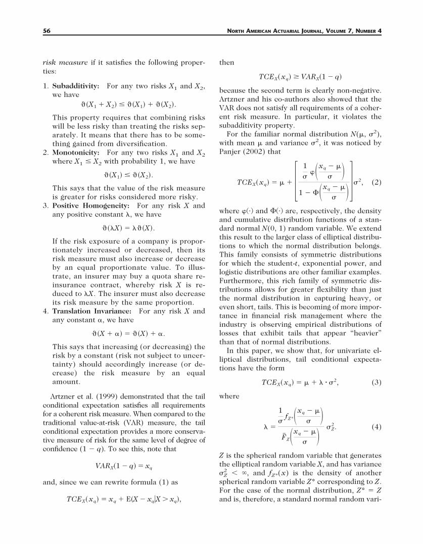
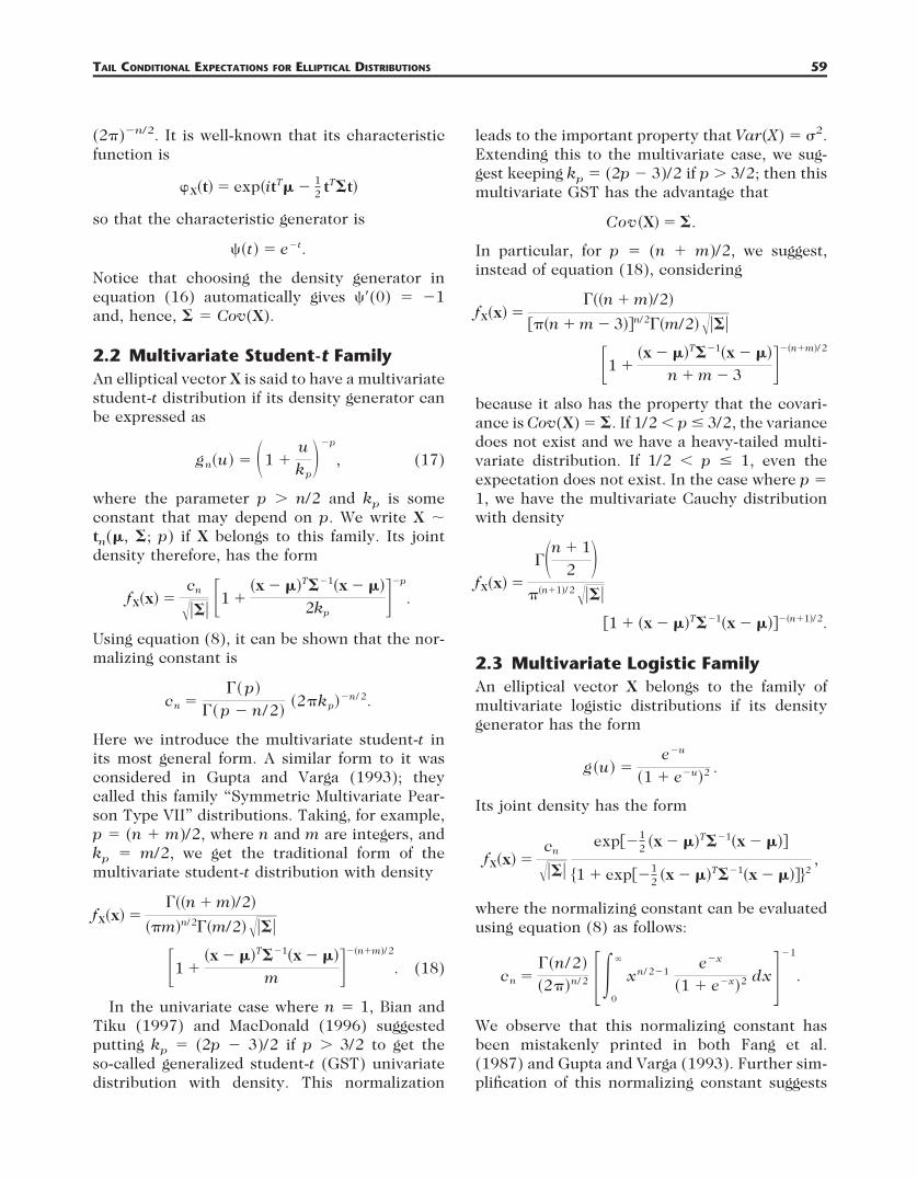
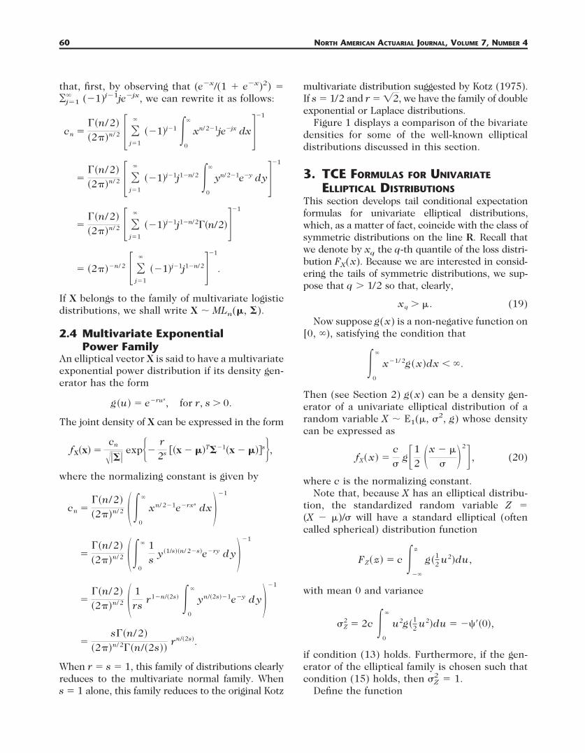
Figure 1 displays a comparison of the bivariatedensities for some of the well-known ellipticaldistributions discussed in this section.

3. TCE FORMULAS FOR UNIVARIATEELLIPTICAL DISTRIBUTIONS

This section develops tail conditional expectationformulas for univariate elliptical distributions,which, as a matter of fact, coincide with the class ofsymmetric distributions on the line R. Recall thatwe denote by xq the q-th quantile of the loss distri-bution FX(x). Because we are interested in consid-ering the tails of symmetric distributions, we sup-pose that q / 1/2 so that, clearly,

xq " (. (19)

Now suppose g(x) is a non-negative function on[0, -), satisfying the condition that

*0

-

x"1/ 2g# x$dx ' -.

Then (see Section 2) g(x) can be a density gen-erator of a univariate elliptical distribution of arandom variable X 2 E1((, )2, g) whose densitycan be expressed as

fX# x$ !c)

g(12 #x # (

) $2) , (20)

where c is the normalizing constant.Note that, because X has an elliptical distribu-

tion, the standardized random variable Z !(X " ()/) will have a standard elliptical (oftencalled spherical) distribution function

FZ# z$ ! c *"-

z

g#12 u2$du,

with mean 0 and variance

)Z2 ! 2c *

0

-

u2g#12 u2$du ! "16#0$,

if condition (13) holds. Furthermore, if the gen-erator of the elliptical family is chosen such thatcondition (15) holds, then )Z

2 ! 1.Define the function


G# x$ ! c *0

x

g#u$du, (21)

which we call the cumulative generator. Thisfunction G plays an important role in our deriva-tion of tail conditional expectations for the classof elliptical distributions. Note that condition(12), which guarantees the existence of the ex-pectation, can equivalently be expressed as

G#-$ ' -.

Define

G! # x$ ! G#-$ # G# x$.

Theorem 1Let X 2 E1((, )2, g) and G be the cumulativegenerator defined in equation (21). Under condition(12), the tail conditional expectation of X is given by

TCEX# xq$ ! ( $ & ! )2, (22)

where & is expressed as

& !

1)

G! #12 zq

2$F! X# xq$

!

1)

G! #12 zq

2$F! Z# zq$

(23)

and zq ! (xq " ()/). Moreover, if the variance ofX exists, or equivalently if equation (13) holds,then (1/)Z

2)G! (12 z2) is a density of another spheri-

cal random variable Z* and & has the form

Figure 1Comparing Bivariate Densities for Some Well-Known Elliptical Distributions


& !

1)

fZ*# zq$

F! Z# zq$)Z

2. (24)

PROOF

Note that

TCEX#xq$ !1

F! X#xq$*

xq

-

x !c)

g(12 ##x # ($/)$2) dx

and, by letting z ! (x " ()/), we have

TCEX# xq$

!1

F! X# xq$*

zq

-

c#( $ )z$ g#12 z2$dz

!1

F! X# xq$ ((F! X# xq$ $ c) *zq

-

zg#12 z2$dz) ,

! ( $ & ! )2,

where

& !1

F! X# xq$!c) *

#1/ 2$ zq2

-

g#u$ du !

1)

G! #12 zq

2$F! Z# zq$

,

which proves the result in equation (23).Now to prove equation (24), suppose condition

(13) holds; that is, the variance of X exists and

12 )Z

2 ! c *0

-

z2g#12 z2$ dz ! *

0

-

zdG#12 z2$ ' -.

Then, [G(12 z2)/G(-)] ! FZ(z) is a distribution

function of some random variable Z with expec-tation given by

E#Z$ !1

G#-$ *0

-

zdG#12 z2$ ! *

0

- (1 #G#1

2 z2$

G#-$) dz

!12 )Z

21

G#-$, -.

Consequently,

*0

-

G! #12 z2$ dz ! 1

2 )Z2

and (1/)Z2)G! (1

2 z2) ! fZ*( z) is a density of

some symmetric random variable Z*, definedon R. e

It is clear that equation (22) generalizes the tailconditional expectation formula derived by Pan-jer (2002) for the class of normal distributions tothe larger class of univariate symmetric distribu-tions. We now illustrate Theorem 1 by consider-ing examples for some well-known symmetric dis-tributions, which include the normal distribution.For the normal distribution, we exactly replicatethe formula developed by Panjer (2002).

1. Normal distribution. Let X 2 N((, )2) sothat the function in equation (20) has the formg(u) ! exp("u). Therefore,

G#x$ ! c *0

x

g#u$ du ! c *0

x

e"u du ! c#1 # e"x$

and1)

G! #12 zq2$ !

c)

exp#" 12 zq

2$! c)

'25*#zq$

!1)

*#zq$,

where it is well-known that the normalizingconstant is c ! (825)"1. Thus, for the normaldistribution, we find )Z

2 ! 1 and

& !

1)

*#zq$

1 # +#zq$, (25)

where *" and +" denote the density anddistribution functions, respectively, of astandard normal distribution. Notice that Z*in Theorem 1 is simply the standard normalvariable Z.

2. Student-t distribution. Let X belong to theunivariate student-t family with a density gen-erator expressed as in equation (17) so that

G#x$ ! cp *0

x

g#u$ du ! cp *0

x #1 $ukp$"p

du

! cp

kp

p # 1 (1 # #1 $xkp$1"p), p / 1,

Here we denote the normalizing constant by cp

with the subscript p to emphasize that it de-pends on the parameter p. Recall from Section2.2 that cp can be expressed as


cp !4#p$

'2kp 4#1/2$4#p # 1/2$

!4#p$

'25kp 4#p # 1/2$. (26)

Note that the case where p ! 1 gives theCauchy distribution for which the mean doesnot exist and, therefore, its TCE also doesnot exist. Now considering the case onlywhere p / 1; we get

1)

G! #12 zq2$!

cp

)

kp

p # 1 #1 $zq

2

2kp$"p.1

. (27)

• Classical student-t distribution. Puttingp ! (m . 1)/2 and kp ! m/2, m ! 1, 2, 3, . . . ,we obtain the univariate student-t distribu-tion with m degrees of freedom (cf. equation18). Then for m / 2, we obtain from equation(27) that

& !

1) ' m

m # 2 fZ#' m # 2m

zq; m # 2$F! Z#zq; m$

,

where fZ(!; m) denotes the density of a stan-dardized classical student-t distribution withm degrees of freedom. If m ! 2, the variancedoes not exist and we have

& !

1)

1

'2fZ# 1

'2zq; 1/2$

F! Z#zq; 2$,

where

fZ#x; 1/2$ !1

#1 $ x2$1/2 ,

which we note is not a density. The casewhere m ! 1 represents the Cauchy distri-bution for which its TCE does not exist.

• Generalized student-t distribution. Forcomparing student-t distributions with differ-ent power parameters p, it is more natural tohave a choice of the normalized coefficient kp

that leads to equal variances. The GST familyhas

kp ! .2p # 3

2 , if p " 3/2

12 , if 1/2 ' p % 3/2

. (28)

In the case where p / 3/2, the variance of Xexists and is equal to Var(X) ! )2, that is, )Z

2

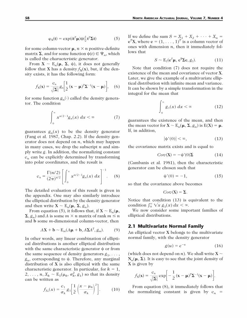
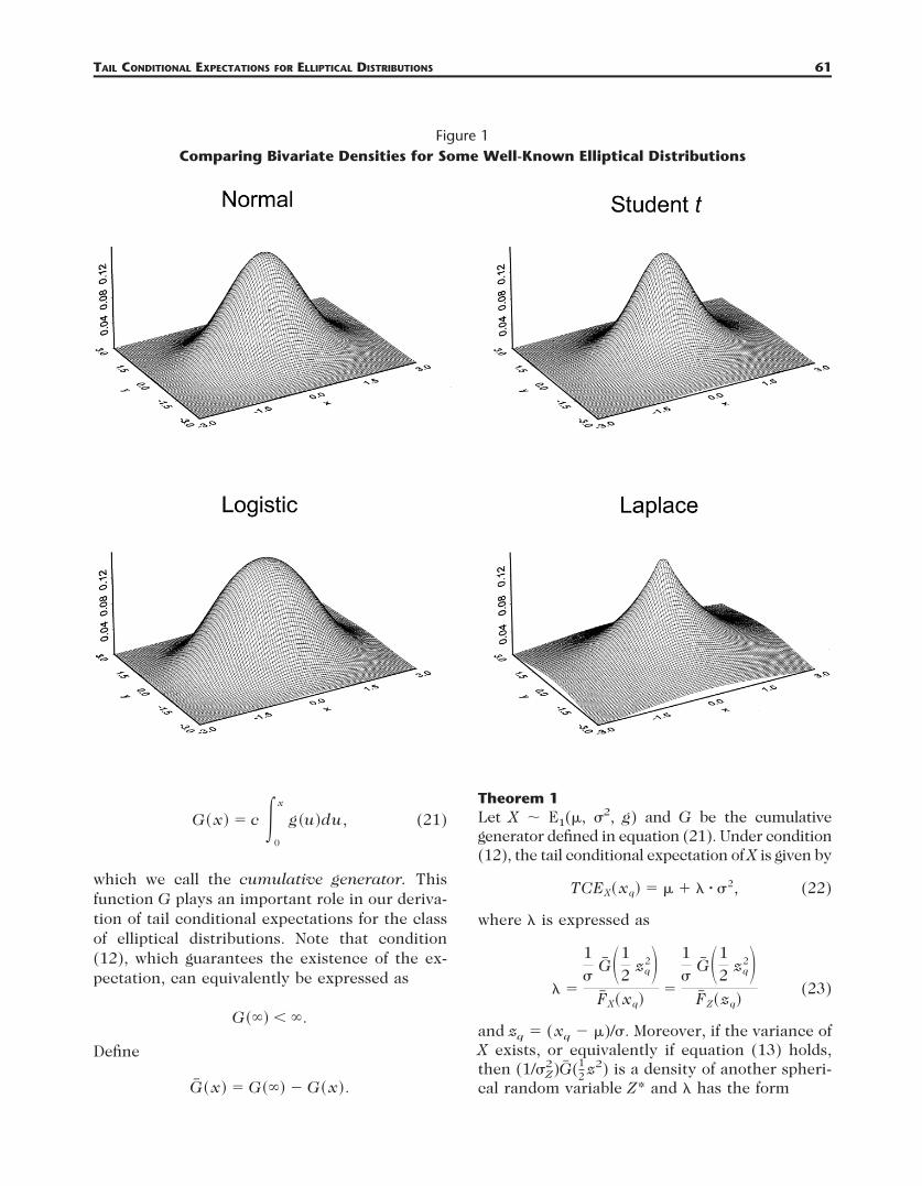
! 1 (see Section 2.2). In the case where 1/2 ,p % 3/2, the variance does not exist and onecan put kp ! 1/2. In Landsman and Makov(1999) and Landsman (2002), credibility for-mulas were examined for this family. Figure 2shows some density functions for the gener-alized student-t distributions with differentparameter values of p. The values of ( and )are chosen to be 0 and 1, respectively. Thesmoothed curve in the figure corresponds tothe case of the standard normal distribution.From equation (27), we have1)

G! #12 zq

2$ !1)

cp

cp"1

kp

#p # 1$

! fZ# 'kp"1

kpzq; p # 1$ , (29)

where fZ(!; p) denotes the density of a stan-dardized GST with parameter p, andkp"1 ! 1/2, cp"1 ! 1/82kp"1 ! 1 when0 , p " 1 % 1/2. For p / 3/2 (the varianceof X exists) from equation (26), it followsthat

cp

cp"1!

4#p$4#p # 3/2$

4#p # 1/2$4#p # 1$ 'kp"1

kp

!#p # 1$

#p # 3/2$ 'kp"1

kp, (30)

and then, from equations (29), (30), and(28),

1)

G! #12 zq2$!

1)

! 'kp"1

kpfZ#'kp"1

kpzq; p # 1$. (31)

Moreover, when p / 5/2, p " 1 / 3/2, so thatwe can re-express equation (31) as follows:

1)

G! #12 zq2$ !

1)

! '2p # 52p # 3 fZ#'2p # 5

2p # 3 zq; p # 1$.Thus, we have

& !

1) '2p # 5

2p # 3 ! fZ#'2p # 52p # 3 zq; p # 1$

F! Z#zq; p$(32)

and Z* is simply a scaled standardized GSTwith parameter p " 1. Notice that (see, e.g.,Landsman and Makov 1999) when p3 -, the


GST distribution tends to the normal distri-bution. It is clear from equation (32) that &will tend to that of the normal distribution inequation (25).

For 3/2 , p % 5/2, 1/2 , p " 1 % 3/2, andtaking into account equation (28), we have

kp"1

kp!

12p # 3 ,

and

& !

1) ' 1

2p # 3 ! fZ# ' 12p # 3 zq; p # 1$

F! Z#zq; p$.

Now, considering the case where 1 , p %3/2, we have 0 , p " 1 % 1/2, (kp"1/kp) !1 and, therefore,

& !

1)

fZ#zq; p # 1$

F! Z#zq; p$.

Notice that, in this case, fZ(zq; p " 1)preserves the form of the density for GST,but it is not a density function because

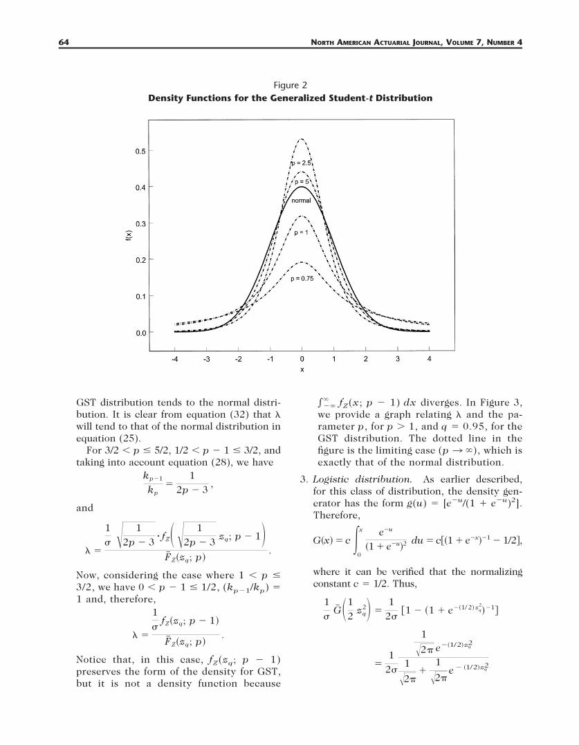
7"-- fZ(x; p " 1) dx diverges. In Figure 3,

we provide a graph relating & and the pa-rameter p, for p / 1, and q ! 0.95, for theGST distribution. The dotted line in thefigure is the limiting case (p 3 -), which isexactly that of the normal distribution.

3. Logistic distribution. As earlier described,for this class of distribution, the density gen-erator has the form g(u) ! [e"u/(1 . e"u)2].Therefore,

G#x$ ! c *0

x e"u

#1 $ e"u$2 du ! c9#1 $ e"x$"1 # 1/2:,

where it can be verified that the normalizingconstant c ! 1/2. Thus,

1)

G! #12 zq

2$ !1

2)91 # #1 $ e"#1/ 2$ zq

2

$"1:

!1

2)

1

'25 e"#1/2$zq2

1

'25$

1

'25e # #1/2$zq

2

Figure 2Density Functions for the Generalized Student-t Distribution


!12

1)

*# zq$

#'25$ # 1 $ *# zq$,

where *" is the density of a standard normaldistribution. Therefore, for a logistic randomvariable, we have the expression for &:

& ! (12

1

#'25$"1 $ *#zq$)

1)

*#zq$

F! Z#zq$,

which resembles that for a normal distribu-tion but with a correction factor.

4. Exponential power distribution. Foran exponential power distribution with adensity generator of the form g(u) !exp("rus) for some r, s / 0, we have

G#x$ ! c *0

x

e"rus du

! c#sr1/s$ # 1*0

rxs

w1/s # 1e # w dw

! c#sr1/s$ # 14#rxs;1/s$,

where

4#z; 1/s$ ! *0

z

w1/s"1e"w dw (33)

denotes the incomplete gamma function.One can determine the normalizing constantto be

c !sr1/#2s$

'2 4#1/#2s$$(34)

by a straightforward integration of the den-sity function. In effect, we have

1)

G! #12 zq2$

!('2r1/s 4(1/(2s)))]"1,4(1/s)"4(r#12 zq

2$ s

;1/s)-and

& !1

F! Z#zq$

1

'2r1/s 4(1/(2s)))

,4(1/s) " 4(r#12 zq2$s

; 1/s)-. (35)

Figure 3The Relationship between % and the Parameter p for the GST distribution


It is clear that, when s ! 1 and r ! 1, thedensity generator for the exponential powerreduces to that of a normal distribution.From equation (34), it follows that c !(825)"1, and from equation (35), it followsthat

& !1

1 # +#zq$#'25$"1(1 # 4#12 zq

2; 1$)!

11 # +# zq$

#'25$"191 # #1 # e"#1/2$zq2$:

!

1)

*# zq$

1 # +# zq$,

which is exactly that of a normal distribution.The Laplace or double exponential distribu-tion is another special case belonging to theexponential power family. In this case, s ! 1/2and r ! 82. From equation (35), it followsthat

& !1

F! Z#zq$

12)

94#2$ # 4#!zq!; 2$:

!1

F! Z#zq$

12) #1 # *

0

!zq!

we"w dw$!

1F! Z#zq$

12)

e"!zq!#1 $ !zq!$

! 21

F! Z#zq$

1)

fZ*#zq$,

where fZ*(z) ! 12 fZ(z)(1 . !z!) ! 1

4 e"!z!(1 . !z!)is density of the new random variable Z*, and)Z

2 ! 2 is a variance of standard double expo-nential distribution that well confirms withequation (24).

4. TCE AND MULTIVARIATE ELLIPTICALDISTRIBUTIONS

Let X ! (X1, X2, . . . , Xn)T be a multivariate ellip-tical vector, that is, X 2 En(", #, gn). Denote the(i, j) element of # by )ij so that # ! /)ij/ i, j!1

n .Moreover, let

FZ# z$ ! c1 *0

z

g1#12 x2$ dx

be the standard one-dimensional distribution func-tion corresponding to this elliptical family and

G# x$ ! c1 *0

x

g1#u$ du (36)

be its cumulative generator. From Theorem 1 andequation (10), we observe immediately that theformula for computing TCEs for each componentof the vector X can be expressed as

TCEXk# xq$ ! (k $ &k ! )k2,

where

&k !

1)k

G! #12 zk,q

2 $F! Z# zk,q$

and zk,q !xq # (k

)k,

or

&k !

1)k

fZ*# zq$

F! Z# zq$)Z

2,

if )Z2 , -.

4.1 Sums of Elliptical RisksSuppose X 2 En(", #, gn) and e ! (1, 1, . . . , 1)T

is the vector of ones with dimension n. Define

S ! X1 $ · · · $ Xn ! &k!1

n

Xk ! eTX, (37)

which is the sum of elliptical risks. We now statea theorem for finding the TCE for this sum.

Theorem 2

The TCE of S can be expressed as

TCES#sq$ ! (S $ &S ! )S2 (38)

where (S ! eT" ! ¥k!1n (k, )S

2 ! eT#e ! ¥i, j!1n

)ij and

&S !

1)S

G! #12 zs,q

2 $F! Z# zS,q$

, (39)

with zS,q ! (sq " (S)/)S. If the covariance matrix ofX exists, &S can be represented by equation (24).


PROOF

It follows immediately from equation (11) thatS 2 En(eT", eT#e, g1), and the result followsusing Theorem 1. e

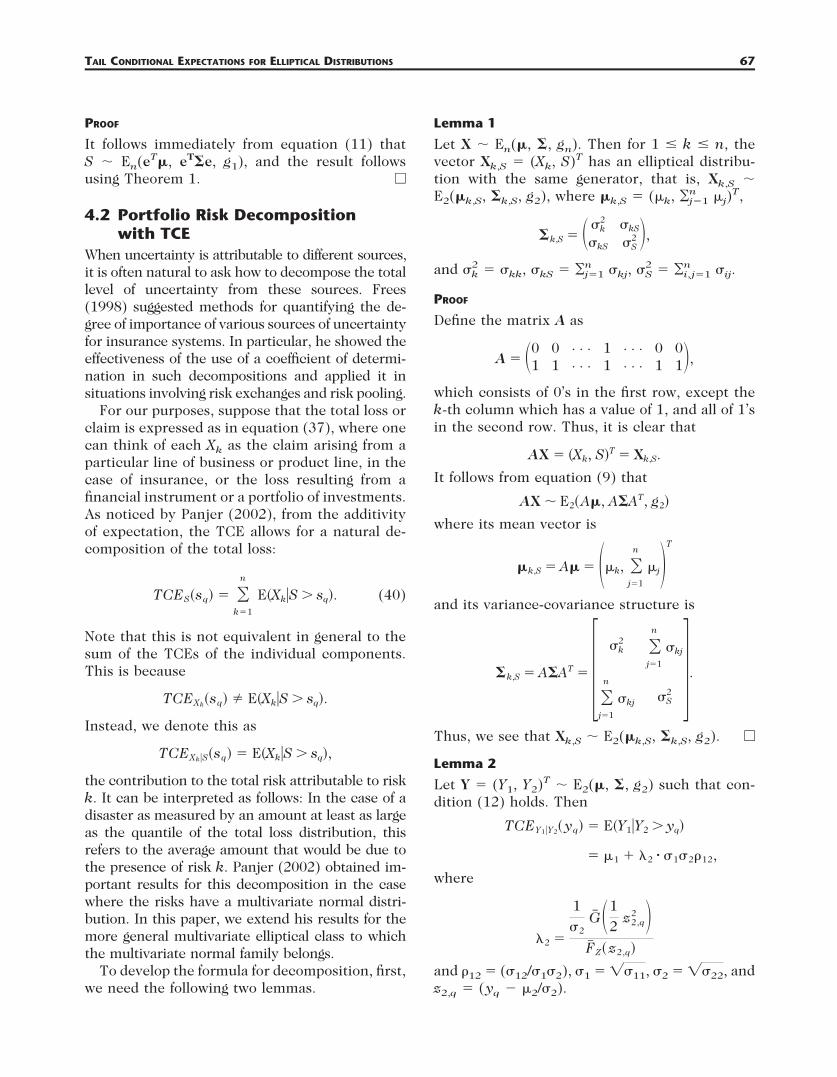
4.2 Portfolio Risk Decompositionwith TCE

When uncertainty is attributable to different sources,it is often natural to ask how to decompose the totallevel of uncertainty from these sources. Frees(1998) suggested methods for quantifying the de-gree of importance of various sources of uncertaintyfor insurance systems. In particular, he showed theeffectiveness of the use of a coefficient of determi-nation in such decompositions and applied it insituations involving risk exchanges and risk pooling.

For our purposes, suppose that the total loss orclaim is expressed as in equation (37), where onecan think of each Xk as the claim arising from aparticular line of business or product line, in thecase of insurance, or the loss resulting from afinancial instrument or a portfolio of investments.As noticed by Panjer (2002), from the additivityof expectation, the TCE allows for a natural de-composition of the total loss:

TCES#sq$ ! &k!1

n

E#Xk!S " sq$. (40)

Note that this is not equivalent in general to thesum of the TCEs of the individual components.This is because

TCEXk#sq$ ( E#Xk!S " sq$.

Instead, we denote this as

TCEXk!S#sq$ ! E#Xk!S " sq$,

the contribution to the total risk attributable to riskk. It can be interpreted as follows: In the case of adisaster as measured by an amount at least as largeas the quantile of the total loss distribution, thisrefers to the average amount that would be due tothe presence of risk k. Panjer (2002) obtained im-portant results for this decomposition in the casewhere the risks have a multivariate normal distri-bution. In this paper, we extend his results for themore general multivariate elliptical class to whichthe multivariate normal family belongs.

To develop the formula for decomposition, first,we need the following two lemmas.

Lemma 1

Let X 2 En(", #, gn). Then for 1 % k % n, thevector Xk,S ! (Xk, S)T has an elliptical distribu-tion with the same generator, that is, Xk,S 2E2("k,S, #k,S, g2), where "k,S ! ((k, ¥j!1

n (j)T,

#k,S ! #)k2 )kS

)kS )S2 $,

and )k2 ! )kk, )kS ! ¥j!1

n )kj, )S2 ! ¥i, j!1

n )ij.

PROOF

Define the matrix A as

A ! #0 0 · · · 1 · · · 0 01 1 · · · 1 · · · 1 1$,

which consists of 0’s in the first row, except thek-th column which has a value of 1, and all of 1’sin the second row. Thus, it is clear that

AX ! #Xk, S$T ! Xk,S.

It follows from equation (9) that

AX + E2#A", A#AT, g2$

where its mean vector is

"k,S ! A" ! #(k, &j!1

n

(j$T

and its variance-covariance structure is

#k,S ! A#AT ! " )k2 &

j!1

n

)kj

&j!1

n

)kj )S2 %.

Thus, we see that Xk,S 2 E2("k,S, #k,S, g2). e

Lemma 2

Let Y ! (Y1, Y2)T 2 E2(", #, g2) such that con-dition (12) holds. Then

TCEY1!Y2# yq$ ! E#Y1!Y2 " yq$

! (1 $ &2 ! )1)2=12,

where

&2 !

1)2

G! #12 z2,q

2 $F! Z# z2,q$

and =12 ! ()12/)1)2), )1 ! 8)11, )2 ! 8)22, andz2,q ! (yq " (2/)2).


PROOF

First note that, by definition, and from equation(6), we have

E#Y1!Y2 " yq$ !1

F! Y2#yq$*

"-

- *yq

-

y1 fY#y1, y2$ dy2dy1

!1

F! Z# z2,q$*

"-

- *yq

-

y1

c2

'!#!

) g2(12 #y # "$T#"1#y # "$) dy2dy1

!1

F! Z# z2,q$) I, (41)

where I is the double integral in equation (41). Inthe bivariate case, we have

!#! ! 0)12 )12

)12 )22 0 ! #1 # =12

2 $)12)2

2

and

#y # "$T#"1#y # "$ !1

#1 # =122 $ (#y1 # (1

)1$2

# 2=12#y1 # (1

)1$#y2 # (2

)2$ $ #y2 # (2

)2$2)

!1

#1 # =122 $ ,(#y1 # (1

)1$ # =12#y2 # (2

)2$)2

$ #1 # =122 $#y2 # (2

)2$2-.

Using the transformations z1 ! (y1 " (1)/)1 andz2 ! (y2 " (2)/)2, and the property that themarginal distributions of multivariate ellipticaldistribution are again elliptical distributions withthe same generator, we have

I !c2

'1 # =122 *

z2,q

- *"-

-

) #(1 $ )1z1$ g2(12

# z1 # =12z2$2

#1 # =122 $

$12 z2

2)dz1dz2

! (1F! Z# z2,q$ $ )1I6, (42)

where

I6 ! *z2,q

- *"-

-

c2

z1

'1 # =122

) g2(12

# z1 # =12z2$2

#1 # =122 $

$12 z2

2)dz1dz2

is the double integral in the second term of theprevious equation. After transformation z6 !(z1 " =12z2)/81 " =12

2 we get

I6 ! '1 # =122 *

z2,q

- *"-

-

c2#z6 $=12z2

'1 # =122 $

) g2(12# z62 $ z2

2$) dz6dz2. (43)

By noticing that the integral of odd function

*"-

-

z6c2g2912 # z62 $ z2

2$: dz6 ! 0,

and again using the property of the marginal el-liptical distribution, giving

*"-

-

c2g2912 # z62 $ z2

2$: dz6 ! c1g1#12 z2

2$,

we have in equation (43)

I6 ! *z2,q

-

=12z2c1g1#12 z2

2$ dz2

! =12 *#1/ 2$ z2,q

2

-

c1g1#u$ du

! =12)2

1)2

G! #12 z2,q

2 $ , (44)

and the result in the theorem then immediatelyfollows from equations (41), (42), and (44). e

Using these two lemmas, we obtain the follow-ing result.

Theorem 3

Let X ! (X1, X2, . . . , Xn)T 2 En(", #, gn) suchthat condition (12) holds, and let S ! X1 . . . . .Xn. Then the contribution of risk Xk, 1 % k % n,to the total TCE can be expressed as


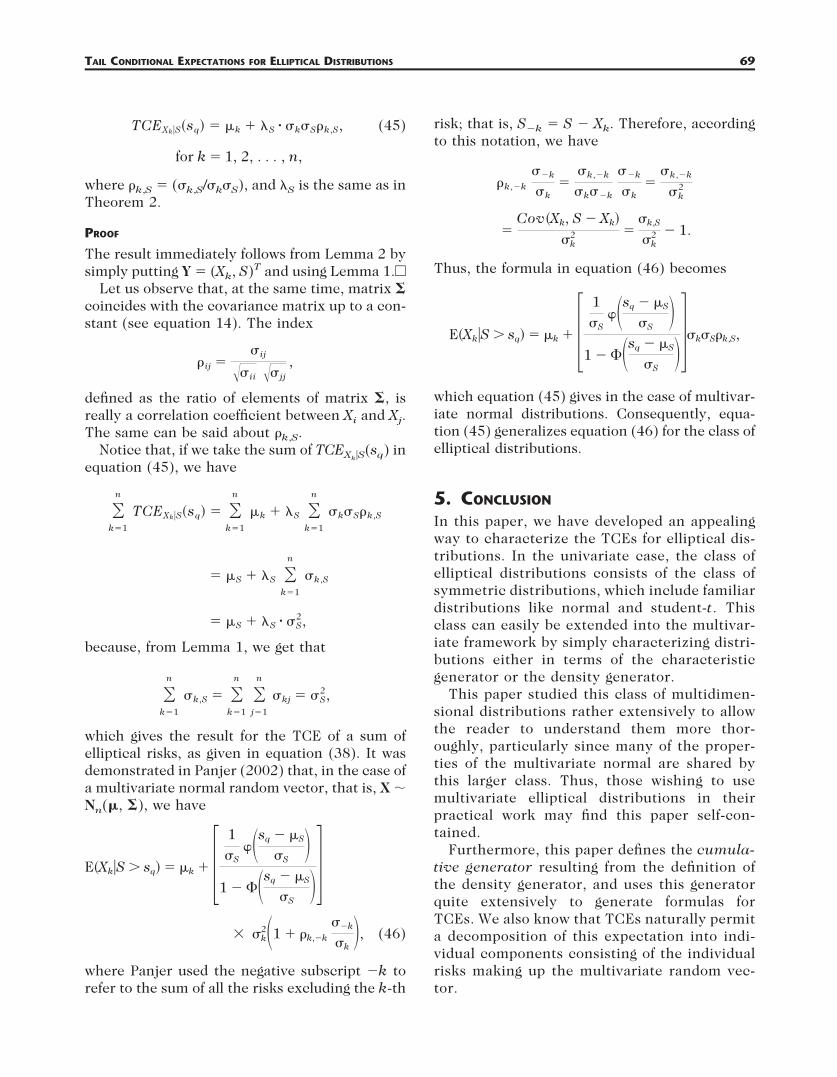
TCEXk!S#sq$ ! (k $ &S ! )k)S=k,S, (45)

for k ! 1, 2, . . . , n,

where =k,S ! ()k,S/)k)S), and &S is the same as inTheorem 2.

PROOF

The result immediately follows from Lemma 2 bysimply putting Y ! (Xk, S)T and using Lemma 1.e

Let us observe that, at the same time, matrix #coincides with the covariance matrix up to a con-stant (see equation 14). The index

=ij !)ij

')ii ')jj,

defined as the ratio of elements of matrix #, isreally a correlation coefficient between Xi and Xj.The same can be said about =k,S.

Notice that, if we take the sum of TCEXk!S(sq) inequation (45), we have

&k!1

n

TCEXk!S#sq$ ! &k!1

n

(k $ &S &k!1

n

)k)S=k,S

! (S $ &S &k!1

n

)k,S

! (S $ &S ! )S2,

because, from Lemma 1, we get that

&k!1

n

)k,S ! &k!1

n &j!1

n

)kj ! )S2,

which gives the result for the TCE of a sum ofelliptical risks, as given in equation (38). It wasdemonstrated in Panjer (2002) that, in the case ofa multivariate normal random vector, that is, X 2Nn(", #), we have

E#Xk!S " sq$ ! (k $ "1)S

*#sq # (S

)S$

1 # +#sq # (S

)S$%

) )k2#1 $ =k,"k

)"k

)k$, (46)

where Panjer used the negative subscript "k torefer to the sum of all the risks excluding the k-th

risk; that is, S"k ! S " Xk. Therefore, accordingto this notation, we have

=k,"k

)"k

)k!

)k,"k

)k)"k

)"k

)k!

)k,"k

)k2

!Cov#Xk, S # Xk$

)k2 !

)k,S

)k2 # 1.

Thus, the formula in equation (46) becomes

E#Xk!S " sq$ ! (k $ "1)S

*#sq # (S

)S$

1 # +#sq # (S

)S$%)k)S=k,S,

which equation (45) gives in the case of multivar-iate normal distributions. Consequently, equa-tion (45) generalizes equation (46) for the class ofelliptical distributions.

5. CONCLUSION

In this paper, we have developed an appealingway to characterize the TCEs for elliptical dis-tributions. In the univariate case, the class ofelliptical distributions consists of the class ofsymmetric distributions, which include familiardistributions like normal and student-t. Thisclass can easily be extended into the multivar-iate framework by simply characterizing distri-butions either in terms of the characteristicgenerator or the density generator.

This paper studied this class of multidimen-sional distributions rather extensively to allowthe reader to understand them more thor-oughly, particularly since many of the proper-ties of the multivariate normal are shared bythis larger class. Thus, those wishing to usemultivariate elliptical distributions in theirpractical work may find this paper self-con-tained.

Furthermore, this paper defines the cumula-tive generator resulting from the definition ofthe density generator, and uses this generatorquite extensively to generate formulas forTCEs. We also know that TCEs naturally permita decomposition of this expectation into indi-vidual components consisting of the individualrisks making up the multivariate random vec-tor.


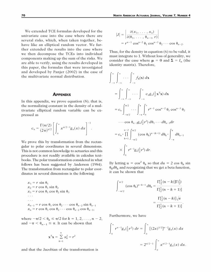
We extended TCE formulas developed for theunivariate case into the case where there areseveral risks, which, when taken together, be-have like an elliptical random vector. We fur-ther extended the results into the case wherewe then decompose the TCEs into individualcomponents making up the sum of the risks. Weare able to verify, using the results developed inthis paper, the formulas that were investigatedand developed by Panjer (2002) in the case ofthe multivariate normal distribution.

APPENDIX

In this appendix, we prove equation (8); that is,the normalizing constant in the density of a mul-tivariate elliptical random variable can be ex-pressed as

cn !4#n/ 2$

#25$n/ 2 (*0

-

xn/ 2"1gn# x$ dx)"1

.

We prove this by transformation from the rectan-gular to polar coordinates in several dimensions.This is not common knowledge to actuaries and thisprocedure is not readily available in calculus text-books. The polar transformation considered in whatfollows has been suggested by Anderson (1984).The transformation from rectangular to polar coor-dinates in several dimensions is the following:

x1 ! r sin >1

x2 ! r cos >1 sin >2

x3 ! r cos >1 cos >2 sin >3

· · ·· · ·xn"1 ! r cos >1 cos >2 · · · cos >n"2 sin >n"1

xn ! r cos >1 cos >2 · · · cos >n"2 cos >n"1,

where "5/2 , >k % 5/2 for k ! 1, 2, . . . , n " 2,and "5 , >n"1 % 5. It can be shown that

xTx ! &k!1

n

xk2 ! r2

and that the Jacobian of the transformation is

!J! ! 0 ?# x1, . . . , xn$

?#>1, . . . , >n"1, r$0

! rn"1 cosn"2 >1 cosn"3 >2 · · · cos >n"2.

Thus, for the density in equation (6) to be valid, itmust integrate to 1. Without loss of generality, weconsider the case where " ! 0 and # ! In (theidentity matrix). Therefore,

*"-

- *"-

-

· · · *"-

-

fX#x$ dx

! *"-

- *"-

-

· · · *"-

-

cngn#12 xTx$ dx

! cn *"5/ 2

5/ 2

· · · *"5

5 *0

-

rn"1 cosn"2 >1 cosn"3 >2

· · · cos >n"2gn#12 r2$ d>1 · · · d>n"1dr

! cn ! 1k!1

n"2 *"5/ 2

5/ 2

(cos >k)n"#k.1$ d>k ! *"5

5

d>n"1

) *0

-

rn"1gn#12 r2$ dr.

By letting u ! cos2 >k so that du ! 2 cos >k sin>kd>k and recognizing that we get a beta function,it can be shown that

*"5/ 2

5/ 2

(cos >k)n"k"1 d>k !491

2 #n # k$:4#12$

4912 #n # k $ 1$:

!491

2 #n # k$:'5

4912 #n # k $ 1$:

.

Furthermore, we have

*0

-

rn"1gn#12 r2$ dr ! *

0

-

9#2x$1/ 2:n"2gn# x$ dx

! 2n/ 2"1 *0

-

xn/ 2"1gn# x$ dx.


Finally, we have

cn ! , 1k!1

n"2 4912 #n # k$:'5

4912 #n # k $ 1$:

! 25

! 2n/ 2"1 *0

-

xn/ 2"1gn# x$ dx-"1

! (4#1$5n/ 2"1

4#n/2$! 25 ! 2n/ 2"1 *

0

-

xn/ 2"1gn#x$ dx)"1

! ( #25$n/ 2

4#n/ 2$ *0

-

xn/ 2"1gn# x$ dx)"1

,

and the desired result follows immediately.

ACKNOWLEDGMENTS

The authors wish to thank the assistance of An-drew Chernih, University of New South Wales, forhelping us produce and better understand thefigures in this article. The first author also wishesto acknowledge the financial support provided bythe School of Actuarial Studies, University of NewSouth Wales, during his visit at the University.

REFERENCES

ANDERSON, T.W. 1984. An Introduction to Multivariate Statisti-cal Analysis. New York: Wiley.

ARTZNER, PHILIPPE, FREDDY DELBAEN, JEAN-MARC EBER, AND DAVID

HEATH. 1999. “Coherent Measures of Risk,” MathematicalFinance 9: 203–28.

BIAN, GUORUI, AND MOTI L. TIKU. 1997. “Bayesian Inference Basedon Robust Priors and MML Estimators: Part 1, SymmetricLocation-Scale Distributions,” Statistics 29: 317–45.

BINGHAM, NICK H., AND RUDIGER KIESEL. 2002. “Semi-ParametricModelling in Finance: Theoretical Foundations,” Quanti-tative Finance 2: 241–50.

CAMBANIS, STAMATIS, S. HUANG, AND G. SIMONS. 1981. “On the The-ory of Elliptically Contoured Distributions,” Journal ofMultivariate Analysis 11: 368–85.

EMBRECHTS, PAUL, ALEXANDER MCNEIL, AND DANIEL STRAUMANN. 2001.“Correlation and Dependence in Risk Management: Prop-erties and Pitfalls,” in Risk Management: Value at Riskand Beyond, edited by M. Dempster and H.K. Moffatt.Cambridge University Press.

———. 1999. “Correlation and Dependence in Risk Manage-

ment: Properties and Pitfalls,” Working paper. Online athttp:/www.math.ethz.ch/finance.

FANG, KAI-TAI, SAMUEL KOTZ, AND KAI WANG NG. 1987. Symmetricmultivariate and related distributions. London: Chapman& Hall.

FELLER, WILLIAM. 1971. An Introduction to Probability Theoryand its Applications. Vol. 2. New York: Wiley.

FREES, EDWARD W. 1998. “Relative Importance of Risk Sources inInsurance Systems,” North American Actuarial Journal2(2): 34–52.

GUPTA, AJAYA K., AND T. VARGA. 1993. Elliptically contoured mod-els in statistics. Netherlands: Kluwer Academic Publishers.

JOE, HARRY. 1997. Multivariate Models and Dependence Con-cepts. London: Chapman & Hall.

HULT, HENRIK, AND FILIP LINDSKOG. 2002. “Multivariate Extremes,Aggregation and Dependence in Elliptical Distributions,”Advances in Applied Probability 34: 587–608.

KELKER, DOUGLAS. 1970. “Distribution Theory of Spherical Distri-butions and Location-Scale Parameter Generalization,”Sankhya 32: 419–30.

KOTZ, SAMUEL. 1975. Multivariate distributions at a cross-road. InStatistical Distributions in Scientific Work, Vol. 1. Editedby G.K. Patil and S. Kotz. D. Reidel Publishing.

KOTZ, SAMUEL, N. BALAKRISHNAN, AND NORMAN L. JOHNSON. 2000.Continuous multivariate distributions. New York: Wiley.

LANDSMAN, ZINOVIY M. 2002. “Credibility Theory: A New Viewfrom the Theory of Second Order Optimal Statistics,” In-surance: Mathematics & Economics 30: 351–62.

LANDSMAN, ZINOVIY M., AND UDI E. MAKOV. 1999. “Sequential Cred-ibility Evaluation for Symmetric Location Claim Distribu-tion,” Insurance: Mathematics & Economics 24: 291–300.

MACDONALD, JAMES B. 1996. “Probability Distributions for Finan-cial Models,” Handbook of Statistics 14: 427–61.

PANJER, HARRY H. 2002. “Measurement of Risk, Solvency Require-ments, and Allocation of Capital within Financial Conglom-erates.” Research Report 01-15 Institute of Insurance andPension Research, University of Waterloo, Waterloo, Ont.

PANJER, HARRY H., AND JING JIA. 2001. “Solvency and Capital Allo-cation.” Research Report 01-14 Institute of Insurance andPension Research, University of Waterloo, Waterloo, Ont.

SCHMIDT, RAPHAEL. 2002. “Tail Dependence for Elliptically Con-toured Distributions,” Mathematical Methods of Opera-tions Research 55: 301–27.

WANG, SHAUN S. 1998. “An Actuarial Index of the Right-TailRisk,” North American Actuarial Journal 2(2): 88–101.

———. 2002. “A Set of New Methods and Tools for EnterpriseRisk Capital Management and Portfolio Optimization.”Working paper, SCOR Reinsurance.

Discussions on this paper can be submitted untilApril 1, 2004. The authors reserve the right to reply toany discussion. Please see the Submission Guidelinesfor Authors on the inside back cover for instructionson the submission of discussions.


every time. Hence, understanding when one ap-proach should be preferred to the other is animportant and interesting area of research. Bra-zauskas and Kaiser (2004) have made a first andvery important step in addressing the issues inthe context of risk measures in actuarial science.

The parametric approach requires the re-searcher to have sufficient confidence in the cho-sen parametric form of the population distribu-tion function F, and there are many of theseforms to choose from (cf., e.g., Kleiber and Kotz2003). When facing this challenge, one mightwonder if the nonparametric approach would beapplicable. The answer naturally depends on thesample size n. In turn, determining whether thesample size is sufficiently large depends on the tailsof the population distribution F and on the dis-tortion function g or, more specifically, on thedistortion parameter r (cf., e.g., the table on p. 50in Jones and Zitikis 2003).

Brazauskas and Kaiser (2004) have done foun-dational research toward a better understandingof the relationship between the sample size n, thedistortion parameter r, and the distribution func-tion F. For example, they argue that, for a certainclass of distribution functions, if the distortionparameter r is at least 0.85, then the sample sizen should at least be 500. Naturally, for smallervalues of r one needs to have larger sample sizesto achieve reliable statistical inferential results.Indeed, the smaller the distortion parameter r is,the more distorted the distribution function Fbecomes in the sense that its tails are madeheavier. It would certainly be of theoretical andpractical interest to obtain a (guiding) formula forchoosing n depending on the value of r, along thelines of the suggestion “if r ! 0.85, then n ! 500”by Brazauskas and Kaiser (2004). This is impor-tant and interesting. Indeed, in the automobileinsurance business, for example, we would expectto have sample sizes well beyond a million orseveral millions. This would allow the researcherto use smaller than, say, r ! 0.85 values of thedistortion parameter and still have reliable statis-tical inferential results using the nonparametricapproach suggested by Jones and Zitikis (2003).If, however, the formula relating the values of rand n would, for a desired value of r, suggest alarger than practically available sample size n,then the parametric approach should be em-ployed.

REFERENCES

BRAZAUSKAS, VYTARAS, AND THOMAS KAISER. 2004. Discussion on“Empirical Estimation of Risk Measures and Related Quan-tities,” North American Actuarial Journal 8(3): 114–17.

JONES, BRUCE L., AND RICARDAS ZITIKIS. 2003. “Empirical Estimationof Risk Measures and Related Quantities,” North AmericanActuarial Journal 7(4): 44–54.

KLEIBER, CHRISTIAN, AND SAMUEL KOTZ. 2003. Statistical Size Dis-tributions in Economics and Actuarial Sciences. Hobo-ken, N.J.: Wiley.

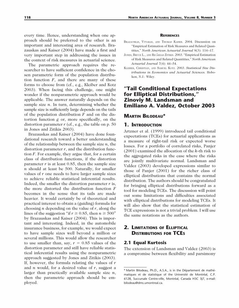
“Tail Conditional Expectationsfor Elliptical Distributions,”Zinoviy M. Landsman andEmiliano A. Valdez, October 2003

MARTIN BILODEAU*

1. INTRODUCTION

Artzner et al. (1999) introduced tail conditionalexpectations (TCEs) for actuarial applications asa measure of right-tail risk or expected worselosses. For a portfolio of correlated risks, Panjer(2001) examined the allocation of the k-th risk tothe aggregated risks in the case where the risksare jointly multivariate normal. Landsman andValdez (2003) developed expressions similar tothose of Panjer (2001) for the richer class ofelliptical distributions that contains the normaldistribution. The authors should be congratulatedfor bringing elliptical distributions forward as atool for modeling TCEs. The discussion will pointout some limitations and difficulties associatedwith elliptical distributions for modeling TCEs. Itwill also show that the statistical estimation ofTCE expressions is not a trivial problem. I will usethe same notations as the authors.

2. LIMITATIONS OF ELLIPTICALDISTRIBUTIONS FOR TCES

2.1 Equal KurtosisThe extension of Landsman and Valdez (2003) isa compromise between flexibility and parsimony

* Martin Bilodeau, Ph.D., A.S.A., is in the Departement de mathe-matiques et de statistique of the Universite de Montreal, C.P.6128, Succursale Centre-ville, Montreal, Canada H3C 3J7, e-mail:[email protected].


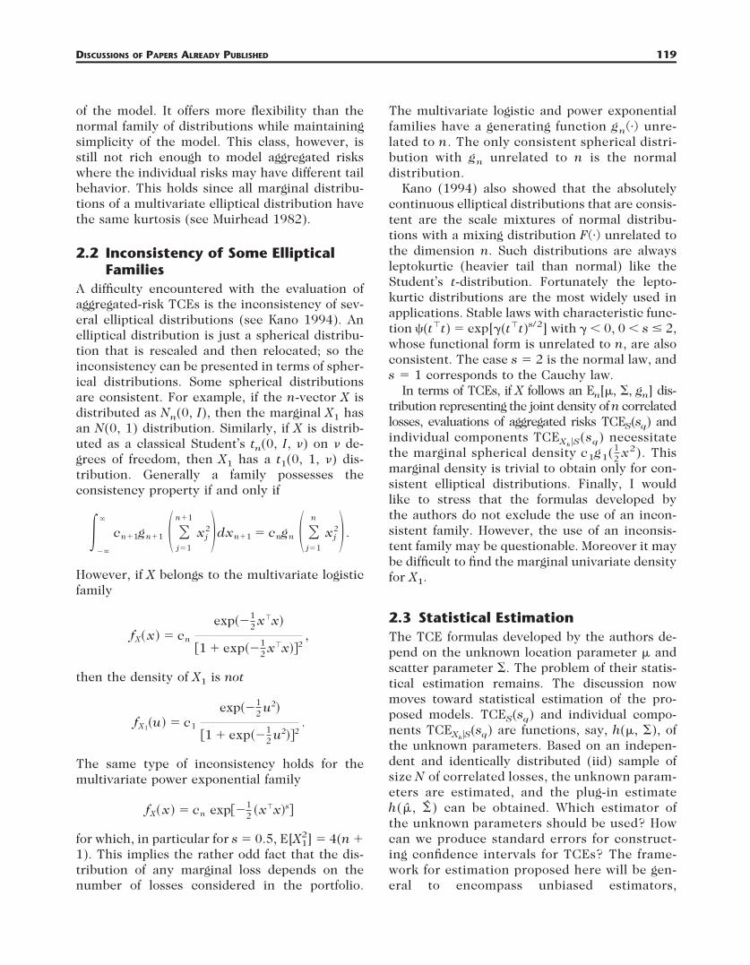
of the model. It offers more flexibility than thenormal family of distributions while maintainingsimplicity of the model. This class, however, isstill not rich enough to model aggregated riskswhere the individual risks may have different tailbehavior. This holds since all marginal distribu-tions of a multivariate elliptical distribution havethe same kurtosis (see Muirhead 1982).

2.2 Inconsistency of Some EllipticalFamilies

A difficulty encountered with the evaluation ofaggregated-risk TCEs is the inconsistency of sev-eral elliptical distributions (see Kano 1994). Anelliptical distribution is just a spherical distribu-tion that is rescaled and then relocated; so theinconsistency can be presented in terms of spher-ical distributions. Some spherical distributionsare consistent. For example, if the n-vector X isdistributed as Nn(0, I), then the marginal X1 hasan N(0, 1) distribution. Similarly, if X is distrib-uted as a classical Student’s tn(0, I, ") on " de-grees of freedom, then X1 has a t1(0, 1, ") dis-tribution. Generally a family possesses theconsistency property if and only if

!#$

$

cn%1gn%1 " #j!1

n%1

xj2$dxn%1 " cngn " #

j!1

n

xj2$ .

However, if X belongs to the multivariate logisticfamily

fX& x' " cn

exp&#12 x!x'

(1 # exp&#12 x!x')2

,

then the density of X1 is not

fX1&u' " c1

exp&#12 u2'

(1 # exp&#12 u2')2

.

The same type of inconsistency holds for themultivariate power exponential family

fX& x' " cn exp(#12 &x!x's)

for which, in particular for s ! 0.5, E[X12] ! 4(n %

1). This implies the rather odd fact that the dis-tribution of any marginal loss depends on thenumber of losses considered in the portfolio.

The multivariate logistic and power exponentialfamilies have a generating function gn! unre-lated to n. The only consistent spherical distri-bution with gn unrelated to n is the normaldistribution.

Kano (1994) also showed that the absolutelycontinuous elliptical distributions that are consis-tent are the scale mixtures of normal distribu-tions with a mixing distribution F! unrelated tothe dimension n. Such distributions are alwaysleptokurtic (heavier tail than normal) like theStudent’s t-distribution. Fortunately the lepto-kurtic distributions are the most widely used inapplications. Stable laws with characteristic func-tion *(t!t) ! exp[+(t!t)s/2] with + , 0, 0 , s $ 2,whose functional form is unrelated to n, are alsoconsistent. The case s ! 2 is the normal law, ands ! 1 corresponds to the Cauchy law.

In terms of TCEs, if X follows an En[-, ., gn] dis-tribution representing the joint density of n correlatedlosses, evaluations of aggregated risks TCES(sq) andindividual components TCEXk%S(sq) necessitatethe marginal spherical density c1g1(1

2 x2). Thismarginal density is trivial to obtain only for con-sistent elliptical distributions. Finally, I wouldlike to stress that the formulas developed bythe authors do not exclude the use of an incon-sistent family. However, the use of an inconsis-tent family may be questionable. Moreover it maybe difficult to find the marginal univariate densityfor X1.

2.3 Statistical EstimationThe TCE formulas developed by the authors de-pend on the unknown location parameter - andscatter parameter .. The problem of their statis-tical estimation remains. The discussion nowmoves toward statistical estimation of the pro-posed models. TCES(sq) and individual compo-nents TCEXk%S(sq) are functions, say, h(-, .), ofthe unknown parameters. Based on an indepen-dent and identically distributed (iid) sample ofsize N of correlated losses, the unknown param-eters are estimated, and the plug-in estimateh(-, .) can be obtained. Which estimator ofthe unknown parameters should be used? Howcan we produce standard errors for construct-ing confidence intervals for TCEs? The frame-work for estimation proposed here will be gen-eral to encompass unbiased estimators,

119DISCUSSIONS OF PAPERS ALREADY PUBLISHED

elliptical maximum likelihood estimators, andaffine invariant robust estimators.

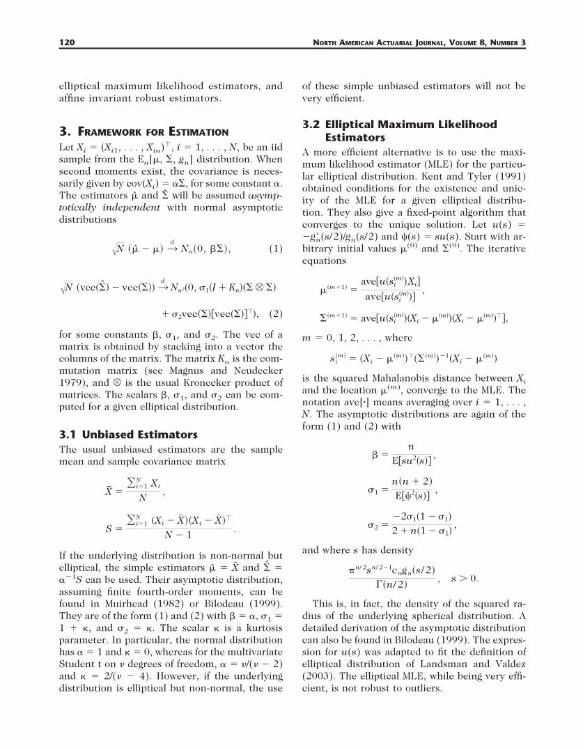
3. FRAMEWORK FOR ESTIMATION

Let Xi ! (Xi1, . . . , Xin)!, i ! 1, . . . , N, be an iidsample from the En[-, ., gn] distribution. Whensecond moments exist, the covariance is neces-sarily given by cov(Xi) ! /., for some constant /.The estimators - and . will be assumed asymp-totically independent with normal asymptoticdistributions

&N &- % -' ¡d

Nn&0, 0.', (1)

&N &vec&.' % vec&.'' ¡d

Nn2&0, 11&I # Kn'&. " .'

# 12vec&.'(vec&.')!', (2)

for some constants 0, 11, and 12. The vec of amatrix is obtained by stacking into a vector thecolumns of the matrix. The matrix Kn is the com-mutation matrix (see Magnus and Neudecker1979), and R is the usual Kronecker product ofmatrices. The scalars 0, 11, and 12 can be com-puted for a given elliptical distribution.

3.1 Unbiased EstimatorsThe usual unbiased estimators are the samplemean and sample covariance matrix

X" "#i!1

N Xi

N,

S "#i!1

N &Xi % X" '&Xi % X" '!

N % 1 .

If the underlying distribution is non-normal butelliptical, the simple estimators - ! X" and . !/#1S can be used. Their asymptotic distribution,assuming finite fourth-order moments, can befound in Muirhead (1982) or Bilodeau (1999).They are of the form (1) and (2) with 0 ! /, 11 !1 % 2, and 12 ! 2. The scalar 2 is a kurtosisparameter. In particular, the normal distributionhas / ! 1 and 2 ! 0, whereas for the multivariateStudent t on " degrees of freedom, / ! "/(" # 2)and 2 ! 2/(" # 4). However, if the underlyingdistribution is elliptical but non-normal, the use

of these simple unbiased estimators will not bevery efficient.

3.2 Elliptical Maximum LikelihoodEstimators

A more efficient alternative is to use the maxi-mum likelihood estimator (MLE) for the particu-lar elliptical distribution. Kent and Tyler (1991)obtained conditions for the existence and unic-ity of the MLE for a given elliptical distribu-tion. They also give a fixed-point algorithm thatconverges to the unique solution. Let u(s) !#g3n(s/2)/gn(s/2) and *(s) ! su(s). Start with ar-bitrary initial values -(0) and .(0). The iterativeequations

-&m%1' "ave(u&si

&m''Xi)

ave(u&si&m'')

,

.&m%1' " ave(u&si&m''&Xi % -&m''&Xi % -&m''!),

m ! 0, 1, 2, . . . , where

si&m' " &Xi % -&m''!&.&m''#1&Xi % -&m''

is the squared Mahalanobis distance between Xi

and the location -(m), converge to the MLE. Thenotation ave[!] means averaging over i ! 1, . . . ,N. The asymptotic distributions are again of theform (1) and (2) with

0 "n

E(su2&s'),

11 "n&n # 2'

E(*2&s'),

12 "#211&1 % 11'

2 # n&1 % 11',

and where s has density

4n/ 2sn/ 2#1cngn&s/ 2'

5&n/ 2', s & 0.

This is, in fact, the density of the squared ra-dius of the underlying spherical distribution. Adetailed derivation of the asymptotic distributioncan also be found in Bilodeau (1999). The expres-sion for u(s) was adapted to fit the definition ofelliptical distribution of Landsman and Valdez(2003). The elliptical MLE, while being very effi-cient, is not robust to outliers.


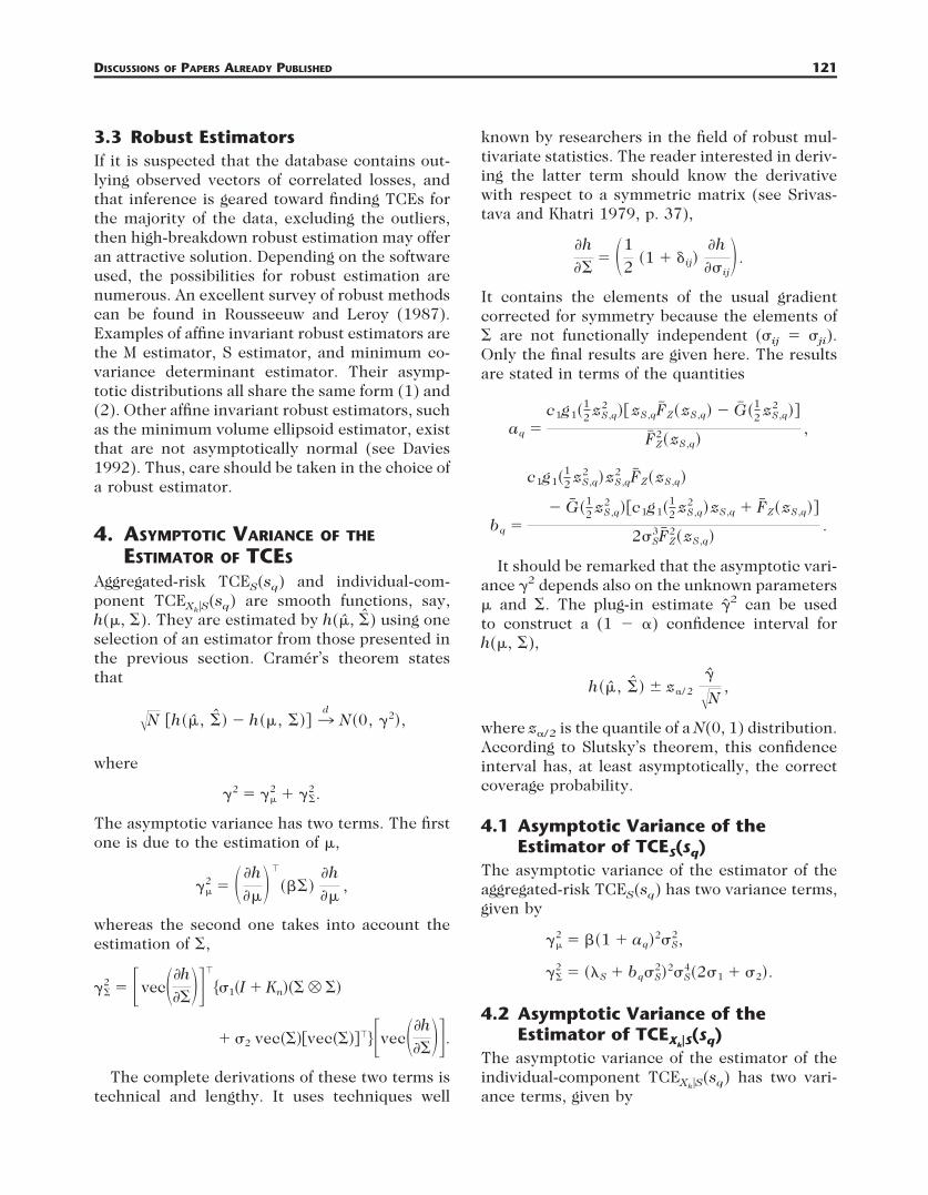
3.3 Robust EstimatorsIf it is suspected that the database contains out-lying observed vectors of correlated losses, andthat inference is geared toward finding TCEs forthe majority of the data, excluding the outliers,then high-breakdown robust estimation may offeran attractive solution. Depending on the softwareused, the possibilities for robust estimation arenumerous. An excellent survey of robust methodscan be found in Rousseeuw and Leroy (1987).Examples of affine invariant robust estimators arethe M estimator, S estimator, and minimum co-variance determinant estimator. Their asymp-totic distributions all share the same form (1) and(2). Other affine invariant robust estimators, suchas the minimum volume ellipsoid estimator, existthat are not asymptotically normal (see Davies1992). Thus, care should be taken in the choice ofa robust estimator.

4. ASYMPTOTIC VARIANCE OF THEESTIMATOR OF TCES

Aggregated-risk TCES(sq) and individual-com-ponent TCEXk%S(sq) are smooth functions, say,h(-, .). They are estimated by h(-, .) using oneselection of an estimator from those presented inthe previous section. Cramer’s theorem statesthat

&N (h&-, .' % h&-, .') ¡d

N&0, +2',

where

+2 " +-2 # +.

2 .

The asymptotic variance has two terms. The firstone is due to the estimation of -,

+-2 " " 6h

6-$!

&0.'6h6-

,

whereas the second one takes into account theestimation of .,

+.2 " 'vec"6h

6.$(!

711&I # Kn'&. " .'

# 12 vec&.'(vec&.')!8'vec"6h6.$(.

The complete derivations of these two terms istechnical and lengthy. It uses techniques well

known by researchers in the field of robust mul-tivariate statistics. The reader interested in deriv-ing the latter term should know the derivativewith respect to a symmetric matrix (see Srivas-tava and Khatri 1979, p. 37),

6h6.

" "12 &1 # 9ij'

6h61ij

$ .

It contains the elements of the usual gradientcorrected for symmetry because the elements of. are not functionally independent (1ij ! 1ji).Only the final results are given here. The resultsare stated in terms of the quantities

aq "c1g1&

12 zS,q

2 '( zS,qF" Z& zS,q' % G" &12 zS,q

2 ')

F" Z2& zS,q'

,

bq "

c1g1&12 zS,q

2 ' zS,q2 F" Z& zS,q'

% G" &12 zS,q

2 '(c1g1&12 zS,q

2 ' zS,q # F" Z& zS,q')

21S3F" Z

2& zS,q'.

It should be remarked that the asymptotic vari-ance +2 depends also on the unknown parameters- and .. The plug-in estimate +2 can be usedto construct a (1 # /) confidence interval forh(-, .),

h&-, .' ' z// 2

+

&N,

where z//2 is the quantile of a N(0, 1) distribution.According to Slutsky’s theorem, this confidenceinterval has, at least asymptotically, the correctcoverage probability.

4.1 Asymptotic Variance of theEstimator of TCES(sq)

The asymptotic variance of the estimator of theaggregated-risk TCES(sq) has two variance terms,given by

+-2 " 0&1 # aq'

21S2,

+.2 " &:S # bq1S

2'21S4&211 # 12'.

4.2 Asymptotic Variance of theEstimator of TCEXk)S(sq)

The asymptotic variance of the estimator of theindividual-component TCEXk%S(sq) has two vari-ance terms, given by


+-2 " 0'1kk # aq"1k,S

2

1S2 $ &2 # aq'( ,

+.2 " 11(:S

2&1S21kk # 1k,S

2 ' # 4:Sbq1S21k,S

2

# 2bq21k,S

2 1S4) # 121k,S

2 &:S # bq1S2'2.

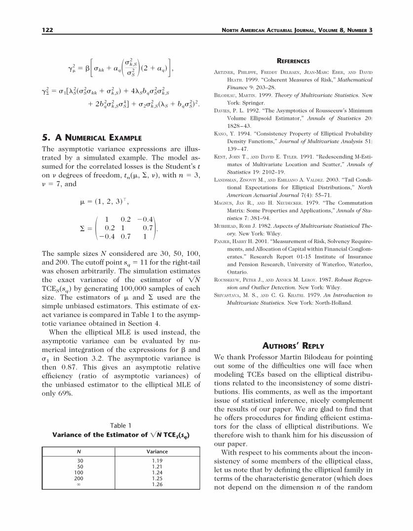
5. A NUMERICAL EXAMPLE

The asymptotic variance expressions are illus-trated by a simulated example. The model as-sumed for the correlated losses is the Student’s ton " degrees of freedom, tn(-, ., "), with n ! 3," ! 7, and

- " &1, 2, 3'!,

. " " 1 0.2 #0.40.2 1 0.7

#0.4 0.7 1$.

The sample sizes N considered are 30, 50, 100,and 200. The cutoff point sq ! 11 for the right-tailwas chosen arbitrarily. The simulation estimatesthe exact variance of the estimator of ;NTCES(sq) by generating 100,000 samples of eachsize. The estimators of - and . used are thesimple unbiased estimators. This estimate of ex-act variance is compared in Table 1 to the asymp-totic variance obtained in Section 4.

When the elliptical MLE is used instead, theasymptotic variance can be evaluated by nu-merical integration of the expressions for 0 and11 in Section 3.2. The asymptotic variance isthen 0.87. This gives an asymptotic relativeefficiency (ratio of asymptotic variances) ofthe unbiased estimator to the elliptical MLE ofonly 69%.

REFERENCES

ARTZNER, PHILIPPE, FREDDY DELBAEN, JEAN-MARC EBER, AND DAVID

HEATH. 1999. “Coherent Measures of Risk,” MathematicalFinance 9: 203–28.

BILODEAU, MARTIN. 1999. Theory of Multivariate Statistics. NewYork: Springer.

DAVIES, P. L. 1992. “The Asymptotics of Rousseeuw’s MinimumVolume Ellipsoid Estimator,” Annals of Statistics 20:1828–43.

KANO, Y. 1994. “Consistency Property of Elliptical ProbabilityDensity Functions,” Journal of Multivariate Analysis 51:139–47.

KENT, JOHN T., AND DAVID E. TYLER. 1991. “Redescending M-Esti-mates of Multivariate Location and Scatter,” Annals ofStatistics 19: 2102–19.

LANDSMAN, ZINOVIY M., AND EMILIANO A. VALDEZ. 2003. “Tail Condi-tional Expectations for Elliptical Distributions,” NorthAmerican Actuarial Journal 7(4): 55–71.

MAGNUS, JAN R., AND H. NEUDECKER. 1979. “The CommutationMatrix: Some Properties and Applications,” Annals of Sta-tistics 7: 381–94.

MUIRHEAD, ROBB J. 1982. Aspects of Multivariate Statistical The-ory. New York: Wiley.

PANJER, HARRY H. 2001. “Measurement of Risk, Solvency Require-ments, and Allocation of Capital within Financial Conglom-erates.” Research Report 01-15 Institute of Insuranceand Pension Research, University of Waterloo, Waterloo,Ontario.

ROUSSEEUW, PETER J., AND ANNICK M. LEROY. 1987. Robust Regres-sion and Outlier Detection. New York: Wiley.

SRIVASTAVA, M. S., AND C. G. KHATRI. 1979. An Introduction toMultivariate Statistics. New York: North-Holland.

AUTHORS’ REPLY

We thank Professor Martin Bilodeau for pointingout some of the difficulties one will face whenmodeling TCEs based on the elliptical distribu-tions related to the inconsistency of some distri-butions. His comments, as well as the importantissue of statistical inference, nicely complementthe results of our paper. We are glad to find thathe offers procedures for finding efficient estima-tors for the class of elliptical distributions. Wetherefore wish to thank him for his discussion ofour paper.

With respect to his comments about the incon-sistency of some members of the elliptical class,let us note that by defining the elliptical family interms of the characteristic generator (which doesnot depend on the dimension n of the random

Table 1Variance of the Estimator of ;N TCES(sq)

N Variance

30 1.1950 1.21

100 1.24200 1.25$ 1.26


vector, although the corresponding density gen-erator may depend on n), one can automaticallyget out of the problem of inconsistency. Further-more, we are pleased to find the nice asymptoti-cally effective estimators for expectations, covari-ance matrices, and TCEs. We wish to emphasizeonly that the problem becomes essentially morecomplicated in the case when the covariance ma-trix does not exist. Then, in this case, the matrixS (using the notation of Professor Bilodeau) be-comes an inconsistent estimator of the matrix .(up to multiplication by any constant), althoughthe vector x"n remains a consistent but very inef-fective estimator of the location vector !. In thecase where the expectations do not exist, x"n isalready an inconsistent estimator of the vector !.In the univariate case, the problem of estimatingthe location parameter - has been discussed inLandsman and Youn (2003). Here the samplemedian has been suggested as an initial value, -0,in the iterative process of estimating -. When thecovariance matrix contains elements that are in-finite, it appears that the problem of finding aneffective estimator of . is not well documented inliterature. However, one can suggest using thesample quantiles as a basis for the estimation (seeLandsman 1996).

We again thank Professor Bilodeau for his dis-cussion of the statistical estimation of TCEs andfor providing the nice numerical example at theend. We would like to add a reference to Csorgoand Zitikis (1996). In this paper the effectivenonparametric estimation of the mean residuallife functional, something closely related to TCEs,was considered.

REFERENCES

CSORGO, MIKLOS, AND RICARDAS ZITIKIS. 1996. “Mean Residual LifeProcesses,” Annals of Statistics 24(4): 1717–39.

LANDSMAN, ZINOVIY M. 1996. “Sample Quantiles and Additive Sta-tistics: Information, Sufficiency, Estimation,” Journal ofStatistical Planning and Inference 52: 93–108.

LANDSMAN, ZINOVIY M., AND HEEKYUNG YOUN. 2003. “Credibility For-mula for the Generalized Student Family.” Proceedings ofthe 7th International Congress of Insurance: Mathe-matics & Economics. Online at http://isfa.univ-lyon1.fr/IME2003/cadres.htm.

“Valuation of Equity-IndexedAnnuities under StochasticInterest Rates,” X. Sheldon Linand Ken Seng Tan, October 2003

MARK D. J. EVANS*The paper presents an analysis of equity index an-nuities reflecting the impact of stochastic interest.This is an important topic. The paper presents ex-tensive formulaic and numerical development. Iwould like to add some comments regarding theinterpretation of some of the results.

1. REMARK 1C

Remark 1c contains the comment, “This is to beexpected because the more volatile the fund is,the greater the appreciation of the fund.” Whilethis statement is not likely to lead the carefulreader astray, a more precise statement is, “Thisis to be expected because the more volatile thefund is, the greater the expected appreciation ofthe fund given that it exceeds the strike.”

2. REMARK 1F

Remark 1f discusses the interaction between inter-est rate volatility and the correlation between inter-est rates and index returns. For the negatively cor-related cases, the participation rates increaseinitially with the volatility of the interest rates. Asthe volatility of the interest rate increases further,the participation rate drops. There is a simple rea-son for this, which is not captured in the paper.There are two forces at work. First, negative corre-lation dampens volatility, thereby reducing optioncosts and increasing participation rates. This tendsto be a first order effect and thus behaves in approx-imately a linear fashion.

The second force at work is the convexity ofoptions. Mathematically, this corresponds to thesecond derivative of option price with respect tointerest rate. From Taylor’s series, this effect isproportional to the square of the change in inter-est rates. This can be seen easily from Table 1where the correlation is 0. The difference in

* Mark D. J. Evans, F.S.A., M.A.A.A., is Vice-President and Actuary atAEGON USA Inc., 400 West Market Street, MC AC-10, Louisville, KY,40202, e-mail: [email protected].


Tail Conditional Expectations for Elliptical Distributions

Documents

Transcript of Tail Conditional Expectations for Elliptical Distributions