
T SYNTHESIZING COMPLEX PROGRAMS F I -O EXAMPLES
31
Published as a conference paper at ICLR 2018 TOWARDS S YNTHESIZING C OMPLEX P ROGRAMS F ROM I NPUT-O UTPUT E XAMPLES Xinyun Chen Chang Liu Dawn Song University of California, Berkeley ABSTRACT In recent years, deep learning techniques have been developed to improve the per- formance of program synthesis from input-output examples. Albeit its significant progress, the programs that can be synthesized by state-of-the-art approaches are still simple in terms of their complexity. In this work, we move a significant step forward along this direction by proposing a new class of challenging tasks in the domain of program synthesis from input-output examples: learning a context-free parser from pairs of input programs and their parse trees. We show that this class of tasks are much more challenging than previously studied tasks, and the test accuracy of existing approaches is almost 0%. We tackle the challenges by developing three novel techniques inspired by three novel observations, which reveal the key ingredients of using deep learning to synthesize a complex program. First, the use of a non-differentiable machine is the key to effectively restrict the search space. Thus our proposed approach learns a neural program operating a domain-specific non-differentiable machine. Second, recursion is the key to achieve generalizability. Thus, we bake-in the notion of recursion in the design of our non-differentiable machine. Third, reinforcement learning is the key to learn how to operate the non-differentiable machine, but it is also hard to train the model effectively with existing reinforcement learning algorithms from a cold boot. We develop a novel two-phase reinforcement learning- based search algorithm to overcome this issue. In our evaluation, we show that using our novel approach, neural parsing programs can be learned to achieve 100% test accuracy on test inputs that are 500× longer than the training samples. 1 I NTRODUCTION Learning a domain-specific program from input-output examples is an important open challenge with many applications (Balog et al., 2017; Reed & De Freitas, 2016; Cai et al., 2017; Li et al., 2017; Devlin et al., 2017; Parisotto et al., 2017; Gulwani et al., 2012; Gulwani, 2011). Approaches in this domain largely fall into two categories. One line of work learns a neural network (i.e., a fully-differentiable program) to generate outputs from inputs directly (Vinyals et al., 2015b; Aharoni & Goldberg, 2017; Dong & Lapata, 2016; Devlin et al., 2017). Despite their promising performance, these approaches typically cannot generalize well to previously unseen inputs. Another line of work synthesizes a non-differentiable (discrete) program in a domain-specific language (DSL) using either a neural network (Devlin et al., 2017; Parisotto et al., 2017) or SMT solvers (Ellis et al., 2016). However, the complexity of programs that can be synthesized using existing approaches is limited. Although many efforts are devoted into the field of neural program synthesis, all of them are still focusing on synthesizing simple textbook-level programs, such as array copying, Quicksort, and a combination of no more than 10 string operations. We believe that the next important step for the community is to consider more complex programs. In this work, we endeavor to pursue this direction and move a big step forward to synthesize more complex programs than before. Along the way, we identify several novel challenges dealing with complex programs that have not been fully discussed before, and propose novel principled approaches to tackle them. First, an end-to-end differentiable neural network is hard to generalize, and in some cases is hard to even achieve a test accuracy that is greater than 0%. We observe that a neural network is too flexible to approximate any functions, but the programs that we want to synthesize typically lie 1
Transcript of T SYNTHESIZING COMPLEX PROGRAMS F I -O EXAMPLES

Published as a conference paper at ICLR 2018
TOWARDS SYNTHESIZING COMPLEX PROGRAMSFROM INPUT-OUTPUT EXAMPLES
Xinyun Chen Chang Liu Dawn SongUniversity of California, Berkeley
ABSTRACT
In recent years, deep learning techniques have been developed to improve the per-formance of program synthesis from input-output examples. Albeit its significantprogress, the programs that can be synthesized by state-of-the-art approaches arestill simple in terms of their complexity. In this work, we move a significant stepforward along this direction by proposing a new class of challenging tasks in thedomain of program synthesis from input-output examples: learning a context-freeparser from pairs of input programs and their parse trees. We show that this classof tasks are much more challenging than previously studied tasks, and the testaccuracy of existing approaches is almost 0%.We tackle the challenges by developing three novel techniques inspired by threenovel observations, which reveal the key ingredients of using deep learning tosynthesize a complex program. First, the use of a non-differentiable machine is thekey to effectively restrict the search space. Thus our proposed approach learns aneural program operating a domain-specific non-differentiable machine. Second,recursion is the key to achieve generalizability. Thus, we bake-in the notion ofrecursion in the design of our non-differentiable machine. Third, reinforcementlearning is the key to learn how to operate the non-differentiable machine, butit is also hard to train the model effectively with existing reinforcement learningalgorithms from a cold boot. We develop a novel two-phase reinforcement learning-based search algorithm to overcome this issue. In our evaluation, we show thatusing our novel approach, neural parsing programs can be learned to achieve 100%test accuracy on test inputs that are 500× longer than the training samples.
1 INTRODUCTION
Learning a domain-specific program from input-output examples is an important open challengewith many applications (Balog et al., 2017; Reed & De Freitas, 2016; Cai et al., 2017; Li et al.,2017; Devlin et al., 2017; Parisotto et al., 2017; Gulwani et al., 2012; Gulwani, 2011). Approachesin this domain largely fall into two categories. One line of work learns a neural network (i.e., afully-differentiable program) to generate outputs from inputs directly (Vinyals et al., 2015b; Aharoni& Goldberg, 2017; Dong & Lapata, 2016; Devlin et al., 2017). Despite their promising performance,these approaches typically cannot generalize well to previously unseen inputs. Another line of worksynthesizes a non-differentiable (discrete) program in a domain-specific language (DSL) using eithera neural network (Devlin et al., 2017; Parisotto et al., 2017) or SMT solvers (Ellis et al., 2016).However, the complexity of programs that can be synthesized using existing approaches is limited.
Although many efforts are devoted into the field of neural program synthesis, all of them are stillfocusing on synthesizing simple textbook-level programs, such as array copying, Quicksort, and acombination of no more than 10 string operations. We believe that the next important step for thecommunity is to consider more complex programs.
In this work, we endeavor to pursue this direction and move a big step forward to synthesize morecomplex programs than before. Along the way, we identify several novel challenges dealing withcomplex programs that have not been fully discussed before, and propose novel principled approachesto tackle them. First, an end-to-end differentiable neural network is hard to generalize, and in somecases is hard to even achieve a test accuracy that is greater than 0%. We observe that a neural networkis too flexible to approximate any functions, but the programs that we want to synthesize typically lie
1

Published as a conference paper at ICLR 2018
in a search space of interest. It is very hard to restrict the learned neural network to always representan instance in the search space. When not, the network is simply overfitting to the training data, andthus cannot generalize. To mitigate this issue, we employ the approach to train a differentiable neuralprogram to operate a domain-specific non-differentiable machine. This combination allows us torestrict the search space by defining the non-differentiable machine, so that any neural program thatcan operate the machine is always a valid program of interest.
Second, the domain-specific machine needs to be expressive enough. In particular, state-of-the-artapproaches, such as RobustFill (Devlin et al., 2017), may fail at tasks involving long outputs becausethey can only synthesize programs of up to 10 string operations, which do not support recursion. Asalso noted by Cai et al. (2017), recursion is a key concept to enable perfect generalization. Therefore,it is desirable that the non-differentiable machine can bake-in the concept of recursion into the design.
Third, the non-differentiable machine makes the model hard to be trained end-to-end, especially whenthe traces to operate the machine are not given during the training. Thus, we rely on a reinforcementlearning algorithm to train the neural program while recovering the execution traces. However, this ischallenging. Previous attempts (Zaremba & Sutskever, 2015) along this direction can only succeedto learn to compute addition of two numbers, and fail even for the tasks of three-number additions.In our evaluation, we observe that training from a cold start is the main difficulty. In particular, themodel trained using existing reinforcement learning algorithms from a cold boot always gets stuckat a local minimum to fit to only a subset of the training samples. More importantly, the recoveredtraces are sometimes “wrong”, which aggravates the issue. To the best of our knowledge, this issueis a long-standing challenging problem for neural program synthesis, and we are not aware of anypromising solution. To tackle this issue, we propose a two-phase reinforcement learning-basedalgorithm. Intuitively, we break up the whole problem into two separate tasks: (1) searching forpossible traces; and (2) training the model with the supervision of traces. Each of these two tasksare easier for reinforcement learning to handle, and we develop a nested algorithm to combine thesolutions to these two tasks to provide the final solution.
To demonstrate our ideas, we propose a novel challenging problem: learning a program to parsean input satisfying an (unknown) context-free grammar into its parse tree. As we will show, thisclass of programs are much more challenging to learn than those considered previously: using moststate-of-the-art approaches, the test accuracy almost remains 0% when the test inputs are longer thanthe training ones. Meanwhile, learning a parser is also an important problem on its own with manyapplications, such as easing the development of domain-specific languages and migrating legacy codeinto novel programming languages. In this sense, this problem exhibits both more complexity andmore practicality than some previously considered problems, such as synthesizing an array-copyingfunction. Therefore, our newly proposed problem serves as a good next step challenge to tackle inthe domain of learning programs from input-output examples.
To implement the idea of learning a neural program operating a non-differentiable machine, we firstdesign the LL machine, which bakes in the concept of recursion in its design. We also design a neuralparsing program, such that every neural parsing program operating an LL machine is restrictedto represent an LL parser. To evaluate our approach, we develop two programming languages, animperative one and a functional one, as two diverse tasks. Combined with our newly proposedtwo-phase reinforcement learning-based algorithm, we demonstrate that for both tasks, our approachcan achieve 100% accuracy on test samples that are 500× longer than training samples, while existingapproaches’ corresponding test accuracies are 0%.
To summarize, our work makes the following contributions: (1) we propose a novel strategy thatcombines training neural programs operating a non-differentiable machine with reinforcement learn-ing, and this strategy allows us to synthesize more complex programs from input-output examplesthan those that can be handled by existing techniques; (2) we reveal three important observations whysynthesizing complex programs can be challenging; (3) we propose a novel two-phase reinforcementlearning-based algorithm to solve the cold start training problem, which may be of independentinterests; (4) we propose the parser learning problem as an important and challenging next step forprogram synthesis from input-output examples that existing approaches fail with 0% accuracy; (5) wedemonstrate that our strategy can be applied to solve the parser learning problem with 100% accuracyon test samples that are 500× longer. We consider applying our strategy to more complex tasks otherthan the parser learning problem as future work.
2

Published as a conference paper at ICLR 2018
a = 1 if x==y Id Id
x y
Input: Output:Eq
If
Id Lit
a 1
Assign
Figure 1: An input-output example. The input is a sequence of tokens [“a", “=", “1", “if", “x",“==", “y"], and the output is its parse tree. The non-terminals are denoted by boxes, and terminals aredenoted by circles.
2 THE PARSING PROBLEM AND APPROACH OVERVIEW
To illustrate our strategy towards synthesizing complex programs, we want to put our presentation ina context. To this end, in this section, we define the parsing problem and outline our approach. Notethat our strategy could also be adapted for other problems. In the following, we start with the formaldefinition of the parsing problem.
Definition 1 (The parsing problem) Assume there exist a context-free language L and a parsingoracle π that can parse every instance in L into an abstract syntax tree. Both L and π are unknown.The problem is to learn a parsing program P , such that ∀I ∈ L, P (I) = π(I).
Figure 1 provides an example of an input and its output parse tree. The internal nodes of the tree arecalled non-terminals, and the leaf nodes are called terminals. The sets of non-terminals and terminalsare disjoint. Each terminal must come from one input token, but the non-terminals do not necessarilyhave such a correspondence. To simplify the problem, we assume the input is already tokenized. Thesets of all non-terminals and terminals can be extracted from the training corpus, i.e., all nodes in theoutput parse trees of training samples. In this work, we assume the vocabulary set (i.e., all terminalsand non-terminals) is finite, and our work can be extended to handle unbounded vocabulary set withtechniques such as pointer networks (Vinyals et al., 2015a).
Remarks. Note that our parsing problem has its counterpart to handle natural languages, which hasbeen extensively studied in the literature (Andor et al., 2016; Chen & Manning, 2014; Yogatama et al.,2016; Dyer et al., 2016). We want to remark on the difference between the two problems. On the onehand, a programming language with a context-free grammar is easier to learn than a natural languagein the sense that the grammar has a rigorous specification to avoid ambiguity. That is, it is alwayspossible to construct a parser to achieve 100% accuracy for a context-free programming language,while this may not be the case for a natural language. On the other hand, learning a programminglanguage parser may be more challenging than a natural language parser, since an instance in aprogramming language can be arbitrarily long, while a natural language sentence typically has only alimited number of words. In this sense, an approach that can learn a natural language parser well maynot be able to handle a programming language, when the test samples are much longer than trainingsamples. As we will observe in our evaluation, this is indeed an issue for existing approaches.
We also want to remark on potential applications of the parsing problem. Nowadays, we need todevelop new domain-specific languages in many scenarios. While the current practice is to developthe grammar and parser manually, this process is error-prone. In our experience, when creatingthe datasets for evaluation, we find that designing a training set of (program, parse tree) pairs istypically easier, but developing the parser takes 2× or 3× more time than developing the trainingset. Intuitively, building a training set only needs developing a tutorial including basic exampleswhose parse trees are easy to construct manually; on the other hand, implementing a parser requiresmuch longer time in debugging, typically with the help of the developed training set. Therefore, ourproposed parser generation problem is a novel practical use case of program-by-example.
Challenges. Learning the parsing program P is challenging for several reasons. First, the cor-respondence between non-terminals and input tokens is unknown. For example, in Figure 1, theparser needs to find out that token “=" corresponds to the non-terminal Assign. Second, the orderof non-terminals in the tree may not align well with the input tokens. For example, in Figure 1,the sub-expression “a=1", which is to the left of the sub-expression “x==y", corresponds to the
3

Published as a conference paper at ICLR 2018
right child of the non-terminal If, which is to the right of the sub-tree corresponding to “x==y"(the sub-tree whose root is the non-terminal Eq). Third, the association of tokens may depend onother tokens. For example, in expressions “x+y*z" and “x+y+z", whether “x+y" forms a sub-treedepends on the operator (i.e., “+" or “*") after it.
Solution overview and paper organization. To tackle the challenges, we make several innovations.First, we employ a paradigm to learn a differentiable neural program operating a non-differentiablemachine in Section 3. In particular, we introduce LL machines (Section 3.1) as an example ofnon-differentiable machine. LL machines can restrict that a learned program always represents aprogram of interest, i.e., an LL parser.
To bake-in the notion of recursion, we think the non-differentiable machine should have a stackstructure and provide CALL and RETURN instructions to simulate recursive calls. In addition, theneural program should operate the machine based on only the stack top to make sure the learnedprogram can generalize. We design the LL machine and neural parsing programs (Section 3.2)to operate an LL machine following these principles. We will show that in doing so, the neuralparsing program can be learned to generalize to longer programs. Note that here we mainly use theLL machines and the neural parsing program to demonstrate that a design supporting recursion isnecessary to achieve generalization, and our strategy is not limited to this combination only.
Third, we design a novel two-phase reinforcement learning-based search algorithm (Section 4) totackle the challenge of training a neural parsing program without the supervision of execution traces.In our evaluation (Section 6), we demonstrate that our approach achieves 100% training accuracy,while the accuracies on all testsets are also 100%. We then discuss related work in Section 7, andconclude in Section 8.
3 NEURAL PROGRAMS OPERATING A NON-DIFFERENTIABLE MACHINE
In this section, we demonstrate how to employ the neural program operating a non-differentiablemachine approach to tackle the neural parsing problem. To carry out this agenda, we first design LLmachines in Section 3.1. The design bakes in the notion of recursion. That is, an LL machine has astack for recursive call stacks, and provides a CALL instruction and a RETURN instruction which canbe used to simulate recursive calls.
Then, we design a neural program operating the LL machine in Section 3.2. We show that the neuralprogram makes its decisions based on only the stack top in the LL machine. In doing so, the neuralprogram can take advantage of the recursion support of an LL machine, and be learned to generalizeto handle longer inputs. We present the details in the following.
3.1 LL MACHINES
We briefly present the design of LL machines. It is inspired by the LL(1) parsing algorithm (Parr &Quong, 1995), and an LL machine is generic enough to allow construct any LL parsers. For example,in our evaluation, we demonstrate that both an imperative language and a functional language can usethe LL machine to construct their parsers.
The LL machine maintains an internal state using a stack of frames and an external state of the streamof input tokens. Each stack frame is an ID-list pair, where the ID is a function ID and in the list are(n, T ) pairs, where T is a parse tree, and n is the root node of T .
An LL machine has five types of instructions: SHIFT, RETURN, CALL, REDUCE, and FINAL. Theirsemantics are presented in Table 1. Intuitively, these instructions can be classified into three classes.The first class, including SHIFT and REDUCE, takes charge of all parser related primitives. In fact,Knuth (1965) has demonstrated that SHIFT and REDUCE primitives are sufficient to construct anycontext-free grammars.
The second class, including CALL and RETURN, is used to operate the stack to simulate recursivecalls. As we will show in the next section, the controller, i.e., a neural parsing program, can decidewhat instruction to execute based on only the stack top frame, whose size can be bounded. This iscrucial for the well-trained neural parsing program to generalize to test samples that are much longerthan training samples.
4

Published as a conference paper at ICLR 2018
SHIFT REDUCE<Id>,(1)Input+𝑦 Id
x
T1Stack
REDUCE<Op+>,(1,3)
Input+𝑦
StackInput𝑥 + 𝑦
Stack0
Input𝑦
StackIdx
T1
SHIFT
CALL1Input𝑦
StackIdx
T1SHIFT
InputEOF
Stack1 (y, y)0 (Id, T1), (+, +)
Idx
T1
REDUCE<Id>,(1)InputEOF
StackIdx
T1Idy
T2RETURN
InputEOF
Stack0 (Id, T1), (+, +), (Id, T2) Id
x
T1Idy
T2
Id Idx y
InputEOF
Stack(Op+, T3)
T3
FINAL
1 2 3
4 5
6 7
8 9
Id Idx y
0
0 (x, x) 0 (Id, T1)
0 (Id, T1), (+, +)
1 (Id, T2)0 (Id, T1), (+, +)
10 (Id, T1), (+, +)
Op+ Op+
Figure 2: A full example to parse x+y into a parse tree. 9 instructions are executed to constructthe final tree. We use red labels to illustrate the changes after performing each operation. For easeof illustration, if a tree has only one node, which is a terminal, then we simply use this terminal torepresent both the root node and the tree in the stack; otherwise, we draw the tree next to the stack,and refer to it with a unique label in the stack.
Insturction Argument Description
SHIFT (None) Pull one token from the input stream to append to the end of thestack top.
REDUCE n, c1, ..., cm
Reduce the stack’s top frame to form a new node rooted at n. cidenotes that the i-th child of the root n is the ci-th elementoriginally in the stack top frame.
CALL fid Push one frame with (fid , []) at the stack top.RETURN (None) Pop the stack top and append the popped data to the new stack top.FINAL (None) Terminate the execution, and return the stack top as the output.
Table 1: LL machine instruction semantics
The third class, including only FINAL, is an instruction to terminate the machine’s execution andproduce the final result. This instruction should be included in any non-differentiable machine design.
Through this design, we want to highlight three key properties in the design of a non-differentiablemachine: instructions for the core functionality related to the programs of interest; instructions toenable recursion; and instructions to produce the results and terminate the machine. We present arunning example using LL machine in Figure 2, and more details and examples to explain how an LLmachine works can be found in Appendix B.
3.2 A NEURAL PARSING PROGRAM
A parsing program operates an LL machine via a sequence of LL machine instructions to parse aninput to a parse tree. Specifically, a parsing program operating an LL machine decides the nextinstruction to execute after each timestep. A key property of the combination of the LL machine andthe parsing program is that its decision can be made based on three components only: (1) the functionID of the top frame; (2) all root nodes of the trees (but not the entire trees) in the list of the top frame;and (3) the next input token. We can safely assume that the list in any stack frame can have at mostK elements (see Appendix B). Here, K is a hyper-parameter of the model. Therefore, the parser onlyneeds to learn a (small) finite number of scenarios in order to generalize to all valid inputs.
To learn the parsing program, we represent it as a neural network, which predicts the next instructionto be executed by the LL machine. Specifically, we consider two inference problems that computethe probabilities of the type and arguments of the next instruction respectively:
p(inst |fid , l, tok) p(arginst |inst ,fid , l, tok)
5
Published as a conference paper at ICLR 2018
Stack top
(Id, 1) (+,+) (Id, 2)
A
𝑒1 𝑒2 𝑒3
A
𝑓𝑖𝑑
A
𝑡𝑜𝑘
fidnext input
token
𝑒0𝑒𝑥
LSTM1 LSTM2
𝐹𝐶 𝐹𝐶
𝑆𝑜𝑓𝑡𝑚𝑎𝑥 𝑆𝑜𝑓𝑡𝑚𝑎𝑥
Instruction Type Call Arguments
LSTM3
𝐹𝐶
𝑆𝑜𝑓𝑡𝑚𝑎𝑥
REDUCE
Arguments 𝑛
Op+
Softm
ax…1, 22, 11, 33, 1…3,2,1
………0.99………
𝑎Op+
REDUCE Arguments 𝑐1, … , 𝑐𝑚
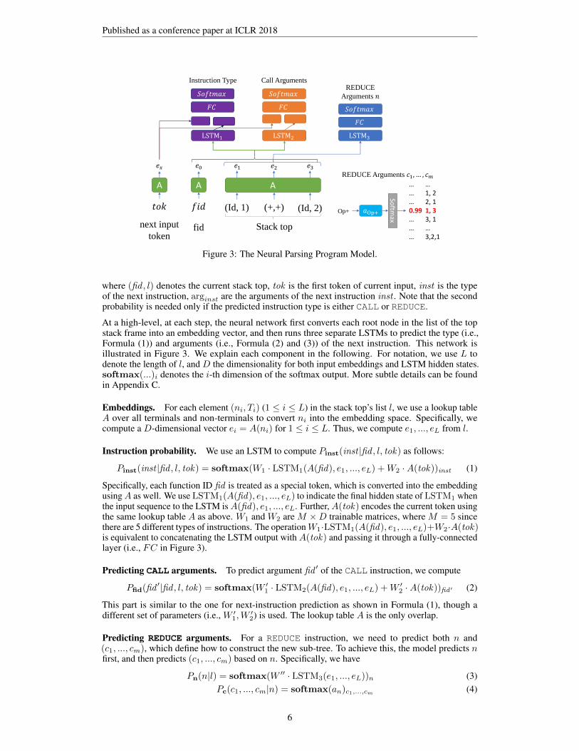
Figure 3: The Neural Parsing Program Model.
where (fid , l) denotes the current stack top, tok is the first token of current input, inst is the typeof the next instruction, arginst are the arguments of the next instruction inst . Note that the secondprobability is needed only if the predicted instruction type is either CALL or REDUCE.
At a high-level, at each step, the neural network first converts each root node in the list of the topstack frame into an embedding vector, and then runs three separate LSTMs to predict the type (i.e.,Formula (1)) and arguments (i.e., Formula (2) and (3)) of the next instruction. This network isillustrated in Figure 3. We explain each component in the following. For notation, we use L todenote the length of l, and D the dimensionality for both input embeddings and LSTM hidden states.softmax(...)i denotes the i-th dimension of the softmax output. More subtle details can be foundin Appendix C.
Embeddings. For each element (ni, Ti) (1 ≤ i ≤ L) in the stack top’s list l, we use a lookup tableA over all terminals and non-terminals to convert ni into the embedding space. Specifically, wecompute a D-dimensional vector ei = A(ni) for 1 ≤ i ≤ L. Thus, we compute e1, ..., eL from l.
Instruction probability. We use an LSTM to compute Pinst(inst |fid , l, tok) as follows:
Pinst(inst |fid , l, tok) = softmax(W1 · LSTM1(A(fid), e1, ..., eL) +W2 ·A(tok))inst (1)
Specifically, each function ID fid is treated as a special token, which is converted into the embeddingusingA as well. We use LSTM1(A(fid), e1, ..., eL) to indicate the final hidden state of LSTM1 whenthe input sequence to the LSTM isA(fid), e1, ..., eL. Further, A(tok) encodes the current token usingthe same lookup table A as above. W1 and W2 are M ×D trainable matrices, where M = 5 sincethere are 5 different types of instructions. The operationW1·LSTM1(A(fid), e1, ..., eL)+W2·A(tok)is equivalent to concatenating the LSTM output with A(tok) and passing it through a fully-connectedlayer (i.e., FC in Figure 3).
Predicting CALL arguments. To predict argument fid ′ of the CALL instruction, we compute
Pfid(fid ′|fid , l, tok) = softmax(W ′1 · LSTM2(A(fid), e1, ..., eL) +W ′2 ·A(tok))fid′ (2)
This part is similar to the one for next-instruction prediction as shown in Formula (1), though adifferent set of parameters (i.e., W ′1,W
′2) is used. The lookup table A is the only overlap.
Predicting REDUCE arguments. For a REDUCE instruction, we need to predict both n and(c1, ..., cm), which define how to construct the new sub-tree. To achieve this, the model predicts nfirst, and then predicts (c1, ..., cm) based on n. Specifically, we have
Pn(n|l) = softmax(W ′′ · LSTM3(e1, ..., eL))n (3)Pc(c1, ..., cm|n) = softmax(an)c1,...,cm (4)
6
Published as a conference paper at ICLR 2018
where LSTM3 is the third LSTM, W ′′ is an N × D trainable matrix. Here N is the number ofdifferent types of non-terminals. Note that different from predicting the next instruction type and theCALL arguments, predicting n does not look at fid and tok , only e1, ..., eL.
The choice of c1, ..., cm is entirely decided by n. To this end, we convert this prediction problemas a one-hot prediction problem. In particular, we encode each possible combination of c1, ..., cminto a unique ID. In fact, given m ≤ K, there are at most f(K) = bK!exp(1) − 1c possibledifferent combinations of c1, ..., cm, where K! is the factorial of K, and exp(1) is the base of theNatural Logarithm (see Appendix C). Therefore, we model the prediction problem of c1, ..., cm as af(K)-way classification problem.
In Equation 4, an is a f(K)-dimensional trainable vector for each n. Assume the ID for (c1, ..., cm)is ξ, then softmax(...)c1,...,cm indicates the ξ-th dimension of the softmax output. Notice thatsetting K to 4 is enough to handle two non-trivial languages used in our evaluation. In both cases,f(K) ≤ 65, which is tractable as the number of classes in a classification problem. We consider tohandle a larger K as future work.
4 LEARNING A NEURAL PARSING PROGRAM
Training a neural parsing program is challenging due to the non-differentiability of the LL machine.The main problem is that the execution trace of the LL machine is unknown, and thus reinforcementlearning is necessary for recovering the execution trace. However, training with reinforcementlearning is very unstable, and is usually stuck at a local minimum that can fit to only a few examples.In such a case, more importantly, the recovered execution traces may be “wrong". To the best of ourknowledge, this is a long-standing open problem, and there is no effective mechanism to find theglobal optimum for a model that can fit to all examples at once.
In this work, we tackle this challenge by proposing a two-phase training strategy. In fact, the mainchallenge of training with a reinforcement learning algorithm lies in the difficulty of jointly recoveringthe execution traces and learning a model with effective parameters. The main idea of our trainingstrategy is to decouple the problem into two phases, where the first phase tries to recover the executiontraces, while the second phase tries to train a set of parameters. In the following, we first explain thehigh-level idea of this two-phase training approach (Section 4.1), and then explain how reinforcementlearning is used (Section 4.2). We will illustrate why and how our algorithm works with a runningexample in Section 5.
4.1 TWO-PHASE TRAINING STRATEGY
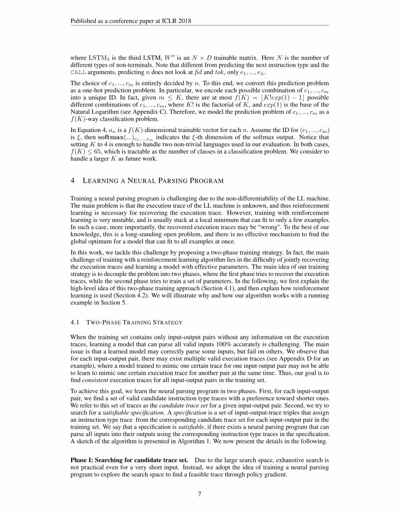
When the training set contains only input-output pairs without any information on the executiontraces, learning a model that can parse all valid inputs 100% accurately is challenging. The mainissue is that a learned model may correctly parse some inputs, but fail on others. We observe thatfor each input-output pair, there may exist multiple valid execution traces (see Appendix D for anexample), where a model trained to mimic one certain trace for one input-output pair may not be ableto learn to mimic one certain execution trace for another pair at the same time. Thus, our goal is tofind consistent execution traces for all input-output pairs in the training set.
To achieve this goal, we learn the neural parsing program in two phases. First, for each input-outputpair, we find a set of valid candidate instruction type traces with a preference toward shorter ones.We refer to this set of traces as the candidate trace set for a given input-output pair. Second, we try tosearch for a satisfiable specification. A specification is a set of input-output-trace triples that assignan instruction type trace from the corresponding candidate trace set for each input-output pair in thetraining set. We say that a specification is satisfiable, if there exists a neural parsing program that canparse all inputs into their outputs using the corresponding instruction type traces in the specification.A sketch of the algorithm is presented in Algorithm 1. We now present the details in the following.
Phase I: Searching for candidate trace set. Due to the large search space, exhaustive search isnot practical even for a very short input. Instead, we adopt the idea of training a neural parsingprogram to explore the search space to find a feasible trace through policy gradient.
7

Published as a conference paper at ICLR 2018
Algorithm 1 A sketch of the two-phase reinforcement learning algorithm1: function SEARCH(Net0, Lesson, TrainingData)2: // Phase 1: nested loop to compute the candidate trace set for each input-output pair3: for (input i, treei) ∈ Lesson do4: Netout ← Net05: for outItr ← 1 to M2 do // Outer loop6: Sample an instruction type trace trace using the policy network Netout
7: Net in ← Netout
8: for InItr ← 1 to M1 do // Inner loop9: Execute the programs following trace and
10: use the policy network Net in to predict the arguments11: T̂ ← Predicted parse tree12: if diff (T̂ , treei) = 0 then13: update the candidate trace set for (input i, treei)14: end if15: Following the REINFORCE algorithm to update Net in
16: end for17: Following the REINFORCE algorithm to update Netout
18: end for19: end for20:21: // Phase 2: find a satisfiable specification22: for (input i, treei) ∈ TrainingData do23: Assume there are d candidate traces for (input i, treei)24: Create θi as a d-dimensional vector and randomly initialize it25: end for26: while True do // It typically terminates within 50 iterations27: for (input i, treei) ∈ TrainingData do28: Sample a candidate trace following the distribution softmax(θi)29: end for30: Train a network Net using reinforcement learning as discussed in Section 4.231: if Training accuracy is 100% then32: return Net33: end if34: end while35: end function
Specifically, we develop a two-nested-loop process to search for the candidate trace set for eachinput-output pair. In each iteration of the outer loop, we run a forward pass of the model to sample anexecution trace including a sequence of instructions and their arguments. We sample the executiontrace using the model described in Section 3.2, except that while sampling the next instruction typeamong valid instruction types, we use the following the distribution instead:
p(inst |fid , l, tok) ∝ softmax(...)inst + σ (5)
Here, σ > 0 is a constant allowing exploration during the search.
After a forward pass, we use the difference between the predicted parse tree and the ground truth asthe reward to update the model’s parameters predicting the next instruction type using policy gradient.This algorithm is referred to as learning without supervision on traces, and we will explain the detailsin Section 4.2.
If the predicted tree is identical to the ground truth, then we have successfully found a valid instructiontype trace, and we add it into the candidate trace set. Otherwise, we test in the inner loops whetherthe sampled instruction type trace is wrong, or only the arguments are predicted wrongly.
To do so, in the inner loops, we use the sampled instruction type trace in the outer loop as thecandidate ground truth, and train the model with weakly supervised learning method which willbe explained in Section 4.2. If any prediction tree during the inner loops matches the candidate
8

Published as a conference paper at ICLR 2018
ground truth, we add the sampled instruction type trace to the candidate set. Otherwise, the model’sparameters are reverted back to those at the beginning of the inner loop, and the sampled instructiontype trace is dropped.
At the end of the outer loop, the candidate trace set is formed, which typically includes 3 to 5instruction type traces, and the model used during the loop is dropped.
In the description of Phase 1 in Algorithm 1, M1 and M2 are two hyper-parameters, where M1 isthe number of iterations for the inner loop, and M2 is the number of iterations for the outer loop.Meanwhile, to escape from a sub-optimal model, we re-initialize the model with the one learned fromthe previous lesson for every M3 iterations in the outer loop. The values of M1, M2 and M3 for ourexperiments are described in Appendix E.
Phase II: Searching for a satisfiable specification. To find a satisfiable specification, again, thenaive idea to perform an exhaustive search requires to explore an exponential number of specificationsin the volume of training samples, which is impractical. For example, if each input-output examplehas 3 candidate traces, the search space of Phase II for a training set of 20 input-output examples has320 = 3, 486, 784, 401 instances.
Alternatively, we employ a sampling-based approach. For each input-output pair (ik, Tk) in thetraining set, we assume Sk = {trk,1, ..., trk,d} is its candidate trace set including d traces. We samplea trace following the distribution
p(trk,j) = softmax(θk)j (6)
where θk is a d-dimensional vector. After one trace is sampled for each input-output pair, these tracesform a specification, and we try to train a model using the weakly supervised learning algorithmdescribed in Section 4.2 with this specification. If the model can correctly parse all inputs, then wefind a satisfiable specification. Otherwise, for each input-output pair (ik, Tk) that is wrongly parsed,we decrease the probability of sampling current trace in the future by updating θk using:
θk ← θk − τ · diff (T̂k, Tk) · ∇θk log p(trk,j) (7)
where T̂k is the predicted parse tree, and τ = 1.0. We observe that such a sampling-based approachcan efficiently sample a satisfiable specification within 30 attempts in our experiments, which couldbe 8 orders of magnitude smaller than the exhaustive search.
Curriculum learning. Searching for a valid trace for a longer input from a randomly initializedmodel can be very hard. To solve this problem, we use curriculum learning to train the model to learnto parse inputs from shorter length to longer length. In the curriculum, the first lesson contains theshortest inputs. In this case, we randomly initialize the model, and train it to parse all samples inLesson 1. Afterwards, for each new lesson, we use the parameters learned from the previous lesson toinitialize the model. When learning each lesson, all training samples from previous lessons are alsoadded into the training set for the current lesson to avoid catastrophic forgetting (Kirkpatrick et al.,2017). Such a process continues until the model can correctly parse all samples in the curriculum.
4.2 TRAINING USING REINFORCEMENT LEARNING
Now we explain how reinforcement learning, especially the policy gradient algorithm REIN-FORCE (Williams, 1992), can be used to update the model during the two-phase training to effectivelyfind a model for both trace exploration and specification satisfiability checking.
In Section 4.1, we explained that we use two versions of the algorithms: learning with no supervisionon traces explores possible execution traces while the ground truth is not given; and weakly supervisedlearning tries to train the model to fit for a given set of trace specifications. The only differencebetween the two algorithms is whether a set of ground truth execution traces is given.
In our experiments, we find that the main challenge to apply the REINFORCE algorithm is that thetraining process is very sensitive to the design of the reward functions. In the following, we firstpresent our design of the reward functions for training the argument prediction sub-networks. In theend, we discuss the different approaches to train the instruction type prediction sub-network whenthe execution traces are given or not. More details can be found in Appendix D.
9

Published as a conference paper at ICLR 2018
Learning to predict REDUCE arguments n and (c1, ..., cm). For the REDUCE instruction, ourintuition is that if a wrong set of arguments is used, the generated sub-tree will look very differentthan the ground truth tree. Therefore, we design the reward function based on the difference betweenthe predicted sub-tree and the ground truth.
First, we define the difference between two trees T and T ′, denoted as diff (T, T ′), to be the editdistance between T and T ′ (Tai, 1979). Assume T̂ is the final generated parse tree and Tg is theground truth output tree. Our goal is to minimize diff (T̂ , Tg), i.e., to 0.
Assume the parse tree constructed by the REDUCE instruction is T̂r. Since the final generated parsetree is composed by these smaller trees, a correct parse tree T̂r should also be a sub-tree of Tg . Basedon this intuition, we define mindiff (T̂r, Tg) = minT∈S(Tg){diff (T̂r, T )}, where S(Tg) indicatesthe set of all sub-trees of Tg . If all of the REDUCE arguments are predicted correctly, mindiff (T̂r, Tg)should be 0.
We design the reward function for n and (c1, ..., cm) as below:
rreduce(T̂r) = − log(α ·mindiff (T̂r, Tg) + β)
where α > 1, β ∈ (0, 1) are two hyperparameters. In our experiments, we choose α = 3, β = 0.01.
In addition, we have a more efficient approach to learn the prediction for n via supervised learning.The details can be found in Appendix D.
Learning to predict CALL argument fid . Designing the reward function to learn the predictionof fid is challenging. As we can see in Figure 5, the choice of each fid affects only the predictionof subsequent instruction types. Our design of the reward function for fid takes this into account.Intuitively, a wrong guess of fid will result in incorrect subsequent predicted instruction types. Basedon this intuition, we design the reward function as follows:
rf (fid(t)) =
t′∑j=t+1
log p( ˆinst(j)|fid (j), l(j), tok (j))inst(j)
where t indicates the current step to execute a CALL instruction, t′ the next step to execute a CALL in-
struction, ˆinst(j)
and inst (j) the predicted and ground truth instruction types, and (fid (j), l(j)), tok (j)
the frame at the stack top and the next input token at step j. Basically, the reward function rfaccumulates the negation of the cross-entropy loss of the predicted instructions from the currentCALL instruction till the next one. More explanations can be found in Appendix D.
Learning to predict the next instruction type. When the execution traces are given, training thenext instruction prediction sub-network is a supervised learning problem, and can be solved usingNPI-style training approaches (Reed & De Freitas, 2016; Cai et al., 2017).
When the execution traces are not given, we use REINFORCE to update the sub-network for nextinstruction type prediction as well. In particular, assume the prediction tree generated during theforward pass is T̂ and the ground truth of the output is Tg . Then the reward function is design to be
− log (α · diff (T̂ , Tg) + β). (8)
5 A RUNNING EXAMPLE
In this section, we detail the design of our reinforcement learning-based algorithm using a runningexample. For illustration purposes, we use a toy language, whose grammar is still challenging to learn.The grammar is very simple: all expressions composed by addition and multiplication. We allow xand y as identifiers and 0 and 1 for literals. We refer to this language as Addition-Multiplication(AM), and it is also a small subset of the WHILE language, which we will evaluate in the next section.The curriculum of AM language is presented below.
10

Published as a conference paper at ICLR 2018
x+ y x ∗ y x+ 0 x ∗ 0 0 + 1 0 ∗ 1y + x+ 0 y + 0 + x 0 + x+ y y ∗ x ∗ 0 y ∗ 0 ∗ x 0 ∗ x ∗ yy ∗ x+ 0 y + x ∗ 0 0 ∗ 1 + x 0 + 1 ∗ x y + 1 + x+ 0 y + 1 + x ∗ 0
y + 1 ∗ x+ 0 y + 1 ∗ x ∗ 0 y ∗ 1 + x+ 0 y ∗ 1 + x ∗ 0 y ∗ 1 ∗ x+ 0 y ∗ 1 ∗ x ∗ 0
The difficulty of the problem: search space. To understand the difficulty of the problem, wewould like to emphasize that learning a correct parser is equivalent to finding the correct executiontrace for each input-output example. On the one hand, if the correct parser is learned, then we canrecover the correct trace for each input-output example by simply executing the parser over the input;on the other hand, if the correct trace of each input-output example is recovered, then we can easilyuse supervised learning to train the parsing program. Therefore, the difficulty of the learning problemcan be measured by the volume of the search space.
We now estimate the size of the entire search space. For AM grammar, we parameterize the LLmachine with K = 3 and F = 3, and there are 4 different non-terminals. We present the number ofthe shortest valid execution traces versus the input length below.
Input length Length of correct exec. traces Number of shortest valid exec. traces3 9 1, 5725 15 2, 771, 7127 21 7, 458, 826, 752
Here, we call an execution trace to be valid if the trace ends with a valid FINAL instruction, but theoutput tree does not necessarily match the ground truth. Meanwhile, we only calculate the numberof traces that are of the same lengths as the correct execution traces, where correct traces mean theshortest traces that can lead to the ground truth output trees. We present the lengths of the shortestcorrect traces above, and denote traces of the same lengths as shortest traces for brevity.
Given our training curriculum, a naive way to find a correct set of execution traces for all input-outputexamples is to perform an exhaustive search over the space of 15726× 277171210× 74588267528 =3.87× 10162. Such a huge search space makes the exhaustive search approach impractical. Noticethat the number of valid execution traces increases exponentially as the input length increases.
Meanwhile, this search space is just for a simple grammar, i.e., AM. For more complex languagesthat we will use in our evaluation, i.e., WHILE and LAMBDA, the value of F and the number ofdifferent non-terminals are larger. Thus, the total number of valid execution traces for WHILE orLAMBDA is much higher than for AM. Also, the average input lengths for WHILE and LAMBDAare 9.3 and 5.6 respectively, which further increases the search space volume significantly.
Motivating the two-phase algorithm. Given the huge search space, we design our techniques toreduce the search space. We observe several aspects why the search space is huge. The first issue isthat the large search space is mainly due to the rule of product when considering the combinationsof traces for all input-output examples. When considering only one input-output example, e.g., aninput of length 7, the size of the search space is around 7.5 billion. Though it is still large, sucha size is more tractable than 3.87 × 10162. This inspires the idea of two-phase learning: the firstphase searches for correct traces for each input-output example, and the second phase searches acombination of traces for different samples. In doing so, the first phase only needs to perform asearch over a space of 6× 1572 + 10× 2771712 + 8× 7458826752 = 5.97× 10¹⁰ instances, whichis still large, but much more amenable than the original search space.
Having done this separation, we can focus on the rest issues: (1) 5.97× 10¹⁰ is still a large searchspace, and thus performing the search in the first phase is not efficient enough yet; and (2) how tomake the second phase efficient and effective is unclear. In the following, we will explain how ourdesign resolves these issues.
Reducing the search space: using instruction type traces instead of execution traces. Weobserve that the total number of the shortest valid execution traces for an input-output example in thecurriculum can be as large as 7.5× 10⁹, which is still large for an exhaustive enumeration. Noticethat most of them are equivalent to each other up to permutation of the instruction arguments. In fact,
11

Published as a conference paper at ICLR 2018
the total number of the shortest valid instruction type traces for each example is much smaller, as weshow below.
Input length Number of shortest valid exec. traces Number of shortest valid inst. type traces3 1, 572 95 2, 771, 712 3827 7, 458, 826, 752 23, 816
Therefore, enumerating valid instruction type traces can be more efficient than enumerating validexecution traces. This observation inspires the nested-loop algorithm in the first phase. In fact, theouter loop uses reinforcement learning to enumerate different instruction type traces, while the innerloop verifies whether an instruction type trace can be instantiated as an execution trace by searchingfor arguments using reinforcement learning. We will defer more discussion about the inner loop later.
Meanwhile, using instruction type traces also helps to reduce the search space of the second phase.For example, among all valid instruction type traces, our training algorithm typically finds 3 to 5traces that can lead to the correct output for each input-output example. Thus, the entire search spaceis of the order of 3n to 5n, where n is the total number of input-output examples being searchedtogether. On the other hand, if all arguments are counted as well, then for each input-output examples,these instruction type traces correspond to tens of execution traces leading to the correct output. Inthis case, the search space is orders of magnitude larger than considering only instruction type traces.Therefore, using instruction type traces is also a key to reduce the size of the search space in thesecond phase.
Reinforcement learning-based sampling versus enumeration. In the first phase, we choose touse reinforcement learning to explore different possibilities of instruction type traces instead ofexhaustive enumeration. This design is based on the following observation. Although we observethat the total number of valid instruction type traces is small for short inputs, this number can growexponentially large when the input length increases. For example, for the WHILE language, amajority of the training inputs have a length larger than 9. In such a case, exhaustively searching overall valid instruction type traces is not efficient, and using a sampling based approach is typically moreeffective. This observation is consistent with previous work (Bergstra & Bengio, 2012; Gulwani et al.,2017). Note that our design of the search process in the second phase is also inspired by the sameobservation.
There is a caveat for both strategies: it may not be easy to know the length of the shortest correctinstruction type traces in advance. In the exhaustive search approach, one can enumerate each lengthof traces in the ascending order and check if there exists a correct instruction type trace. Using areinforcement learning approach, this process could be reversed: since each outer loop may samplean arbitrarily long instruction type trace, it may sample several longer instruction type traces beforereaching the ones with the minimal length. This may cause our reinforcement learning algorithm torun longer for a short input; but for a long input, the sampling approach typically can find the set ofcandidate instruction type traces much sooner than using the exhaustive enumeration approach. Inour evaluation, we observe that typically setting M2 = 10, 000 is sufficiently large to find a good setof candidate traces regardless of the input length.
There is a side benefit of using a reinforcement learning-based sampling in the outer loop: the sameRL framework can be used in the inner loop to search for a valid execution trace instantiation fromthe instruction type trace. Thus, the RL algorithm can also be used as an efficient verification tool tocheck whether a valid instruction type trace is correct or not.
The effectiveness of training curriculum. The training curriculum helps with the training in threeaspects. First, the RL algorithm has a caveat: for a long input, RL algorithm cannot find even onecorrect instruction type trace from a cold start. Thus, curriculum learning can help to mitigate thisissue. In particular, when searching for correct instruction type traces for an example in one lesson,the model is initialized with parameters that can fit to all examples in previous lessons. In doing so,the RL algorithm can effectively skip many obviously bad traces, and thus find the correct ones moreefficiently.
Second, the training curriculum can also help RL to skip those instruction type traces that are correctfor the examined input-output examples, but are inconsistent with other examples in previous lessons.For our AM language, we provide the number of correct instruction traces as well as the number of
12

Published as a conference paper at ICLR 2018
Example # of correct Example # of correct Example # of correcttraces traces traces
x + y 9 (3) x * y 9 (3) x + 0 9 (3)x * 0 9 (3) 0 + 1 9 (3) 0 * 1 9 (3)
y + x + 0 99 (11) y + 0 + x 99 (11) 0 + x + y 99 (11)y * x * 0 99 (11) y * 0 * x 99 (11) 0 * x * y 99 (11)y * x + 0 99 (11) y + x * 0 81 (9) 0 * 1 + x 99 (11)0 + 1 * x 81 (9) y + 1 + x + 0 1107 (41) y + 1 + x * 0 891 (33)
y + 1 * x + 0 1053 (39) y + 1 * x * 0 891 (33) y * 1 + x + 0 1107 (41)y * 1 + x * 0 891 (33) y * 1 * x + 0 1107 (41) y * 1 * x * 0 1107 (41)
Table 2: The numbers of correct instruction traces and instruction type traces for each example in theAM training set. The two numbers are provided in the column of “# of correct traces" in the form ofn(m), where n (outside the brackets) indicates the number of instruction traces, and m (inside thebrackets) indicates the number of instruction type traces.
correct instruction type traces for each example in Table 2. From the table, we can observe that thenumber of correct traces increases significantly with respect to the increase of the input length. Usingcurriculum training, we can reduce the number of candidate instruction type traces to be 3 to 5 foreach example regardless of the input length, which thus further reduces the search space for Phase II.
Third, it can further reduce the search space of the second phase. Assume the algorithm finds 3candidate instruction type traces for each input-output pair. Since there are 24 examples in the trainingset, the search space of the second phase can be as large as 324 = 2.82× 10¹¹. When following thetraining curriculum, each lesson may have only 6 examples. Thus, the search space for each lesson inthe second phase can be as few as 36 = 729, i.e., 8 orders of magnitude smaller. When training on thenext lesson, since the instruction type traces for examples in previous lessons have been determined,the search can focus on the current lesson. Therefore, using a training curriculum can further reducethe search space while guaranteeing that the model is not overfitting to a subset of examples.
6 EVALUATION
To show that our approach is general and able to learn to parse different types of context-freelanguages using the same architecture and approach, we evaluate our approach on two tasks to learna parser for an imperative language WHILE and an ML-style (Milner, 1997) functional languageLAMBDA respectively. WHILE and LAMBDA contain 73 and 66 production rules, and their parsingprograms can be implemented in 89 and 46 lines of Python code respectively. Notice that theseprograms are more sophisticated than previous studied examples. For example, Quicksort studiedin (Cai et al., 2017) can be implemented in 3 lines of Python code, and FlashFill tasks studiedin (Devlin et al., 2017; Parisotto et al., 2017) can be implemented in 10 lines of code in their DSL.Grammar specifications of the two languages are presented in Appendix G and H respectively.
For each task, we prepare three training sets: (1) Curriculum: a well-designed training curriculumincluding 100 to 150 examples that enumerates all language constructors; (2) Std-10: a training setincludes all examples in the curriculum, and also 10,000 additional randomly generated inputs withlength 10 on average; and (3) Std-50: a training set includes all examples in the curriculum, and also1,000,000 additional randomly generated inputs with length 50 on average. In all datasets, all groundtruth parse trees are provided. Note that once our model learns to parse all inputs in the curriculum, itcan parse all inputs in training sets (2) and (3) for free. We include two standard training sets, i.e.,Std-10 and Std-50, to allow a fair comparison against baseline approaches, which typically require alarge amount of training data.
We compare our approach with two sets of baselines. The first class of approaches learn end-to-end neural network models as the program. This class includes a sequence-to-sequence approach(seq2seq) (Vinyals et al., 2015b), a sequence-to-tree (seq2tree) approach (Dong & Lapata, 2016), andLSTM with unbounded memory (Grefenstette et al., 2015). In particular, we evaluate all three variantsproposed in (Grefenstette et al., 2015). The second class includes the state-of-the-art approach forneural program synthesis, i.e., RobustFill (Devlin et al., 2017), which learns a discrete program in aDSL.
13

Published as a conference paper at ICLR 2018
While-Lang
Train Test Ours Seq2seq Seq2tree Stack Queue DeQue Robust-
LSTM LSTM LSTM Fill(Projected)
Cur
ricu
lum
Training 100% 81.29% 100% 100% 100% 100% 13.67%Test-10 100% 0% 0.8% 0% 0% 0% 0%
Test-100 100% 0% 0% 0% 0% 0% 0%Test-1000 100% 0% 0% 0% 0% 0% 0%Test-5000 100% 0% 0% 0% 0% 0% 0%
Std-
10
Training 100% 94.67% 100% 81.01% 72.98% 82.59% 0.19%Test-10 100% 20.9% 88.7% 2.2% 0.7% 2.8% 0%
Test-100 100% 0% 0% 0% 0% 0% 0%Test-1000 100% 0% 0% 0% 0% 0% 0%
Std-
50
Training 100% 87.03% 100% 0% 0% 0% 0.0019%Test-50 100% 86.6% 99.6% 0% 0% 0% 0%
Test-500 100% 0% 0% 0% 0% 0% 0%Test-5000 100% 0% 0% 0% 0% 0% 0%
Lambda-Lang
Train Test Ours Seq2seq Seq2tree Stack Queue DeQue Robust-
LSTM LSTM LSTM Fill(Projected)
Cur
ricu
lum
Training 100% 96.47% 100% 100% 100% 100% 29.21%Test-10 100% 0% 0% 0% 0% 0% 0%
Test-100 100% 0% 0% 0% 0% 0% 0%Test-1000 100% 0% 0% 0% 0% 0% 0%Test-5000 100% 0% 0% 0% 0% 0% 0%
Std-
10
Training 100% 93.53% 100% 0% 95.93% 2.23% 0.26%Test-10 100% 86.7% 99.6% 0% 6.5% 0.1% 0%
Test-100 100% 0% 0% 0% 0% 0% 0%Test-1000 100% 0% 0% 0% 0% 0% 0%
Std-
50
Training 100% 66.65% 89.65% 0% 0% 0% 0.0026%Test-50 100% 66.6% 88.1% 0% 0% 0% 0%
Test-500 100% 0% 0% 0% 0% 0% 0%Test-5000 100% 0% 0% 0% 0% 0% 0%
Table 3: Experimental results on While-Lang and Lambda-Lang dataset. We evaluate our approach(ours), seq2seq (Vinyals et al., 2015b), seq2tree (Dong & Lapata, 2016), with Stack LSTM, QueueLSTM and DeQue LSTM from (Grefenstette et al., 2015). “Std-10" indicates the standard training setwith 10,000 samples of length 10, “Std-50” indicates the standard training set with 1,000,000 samplesof length 50, and “Curriculum" indicates the specially designed learning curriculum. “Test-LEN"indicates the testset including inputs of length LEN.
For testing, we create six levels of testsets, i.e., Test-10, Test-50, Test-100, Test-500, Test-1000 andTest-5000, where each input has 10, 50, 100, 500, 1000 and 5000 tokens on average respectively. Eachtest set contains 1000 randomly generated expressions. We guarantee that test data does not overlapwith training samples. Table 3 shows experimental results on WHILE and LAMBDA languages. Wediscuss the results below.
Observations on our approach. We observe that once our neural parsing program is trained toachieve 100% accuracy on the training data, it can always achieve 100% test accuracy on arbitrarytest samples regardless of their lengths.
We emphasize that all the results of our approach are achieved by using the curriculum learningapproach. Without curriculum training, our approach cannot train any effective models, and thetest accuracy is 0% when the test input is longer than training inputs. Also, we observe that ourtwo-phase training algorithm can always make the neural network be trained to achieve 100% on the
14

Published as a conference paper at ICLR 2018
curriculum training set. Further, in our evaluation, we observe that the training curriculum is veryimportant to regularize the reinforcement learning process.
Therefore, our evaluation demonstrates that the combination of our three ideas enables us to learn aprogram to achieve 100% accuracy on test samples that can be even 500× longer than the trainingones, while baseline approaches are hard to even achieve a test accuracy that is greater than 0%.
Observations on approaches to learn end-to-end neural network models. We first observe thatwhen the length of test samples is larger than training ones, the test accuracy drops to 0% regardlessof the end-to-end differential approach being evaluated. This illustrates that none of these approachescan generalize to longer inputs. As we have explained, it is very hard to enforce the learned model toalways represent a parser to handle arbitrarily long inputs. Thus even the well-trained models simplyoverfit to the training samples, and cannot generalize to longer inputs.
Also, when training on the curriculum dataset, no approaches can generalize to any test data. Thisis simply because the training set contains too few instances, so that the overfitting phenomenonexplained above becomes more prominent.
When test samples are of the same length as training ones and training with the standard trainingsets, we observe that seq2tree performs better than seq2seq. We attribute this phenomenon to thereason that the seq2tree model essentially employs the recursion idea in its decoder design. In fact, inthe decoding phase, different from seq2seq, which generates the entire sequence at once, seq2treetraverses down along the paths from the root to leaves and recursively decodes each layer of theparse tree along a path. On WHILE and LAMBDA tasks, it can even achieve an accuracy of almost100% on Test-50 and Test-10 respectively, showing that this recursive decoding approach is effective.However, the encoding phase of seq2tree is not recursive. This hinders its generalization to longerinputs.
Meanwhile, for both seq2seq and seq2tree models, when they are trained on Std-50 training set, thegap between the training accuracy and the test accuracy is much smaller than the ones trained onStd-10 training set. For example, on WHILE dataset, the test accuracy of seq2seq is around 20%on Test-10; however, when trained on Std-50, it can reach an accuracy of above 85% on Test-50.This observation suggests that the models overfit to the Std-10 training set. When Std-50 is used fortraining, on the other hand, the overfitting issue is mitigated. In addition, we notice that while the testaccuracy for the WHILE task increases when Std-50 is used for training, it drops for the LAMBDAtask. We attribute it to the fact that the size of the parse tree in LAMBDA language is much largerthan the parse tree in WHILE language given the input with the same number of tokens. Thus, whenthe inputs get longer, the model is harder to fit to the parse trees of larger sizes.
We also observe that models proposed in (Grefenstette et al., 2015) perform poorly, and much worsethan the other two end-to-end neural network approaches. Grefenstette et al. (2015) proposes LSTMdecoders with unbounded memory to generalize the idea of neural pushdown automaton, whichwas designed to handle the parsing tasks. Our results show that when these models are trained onStd-10, they suffer severely from overfitting. Further, when trained on Std-50, the training accuracydrops to 0%. We attribute the poor performance to the fact that the production and transduction rulesdeveloped in the two evaluated languages are too complex for such architectures to learn effectively.In fact, Grefenstette et al. (2015) reports that all three proposed approaches perform poorly on thebi-gram flipping task, which is a much simpler sub-task of the two languages in consideration. Thisfurther illustrates the challenges of training such end-to-end differentiable neural networks to simulateeven simple data structures such as stacks or queues.
Observations on approaches to synthesize discrete programs. Note that the training of Robust-Fill, as described in (Devlin et al., 2017), do not use the input-output examples in the training set,but construct their own training set instead. The source code of RobustFill is not available, and ourre-implementation cannot produce any meaningful programs.
To make a fair comparison, we compute a projected accuracy which is the accuracy that can beachieved by the most effective program in the space of the RobustFill DSL. Note that given RobustFillcan produce programs of length of up to 10, the entire output program space of RobustFill is finite,though exponentially large. However, we notice that we can efficiently enumerate the small sub-set
15

Published as a conference paper at ICLR 2018
of effective programs using a simple heuristic to cut ineffective constructors in a program. We detailthe algorithm in Appendix K.
The results in Table 3 report an upper bound of the accuracy that can be achieved by the RobustFillapproach. We can observe that the best program in the RobustFill DSL space can only fit to asmall subset of the training data, and cannot generalize to longer test inputs due to the length of theprograms is limited. Essentially, the outputs of a program in the RobustFill DSL space are boundedby the length of the program itself (see Appendix K for a discussion), while the outputs of our parsingproblem can grow arbitrarily long. When the test samples become longer, the RobustFill approachwill soon fail with 0% accuracy.
Therefore, to make the RobustFill approach able to handle our parsing task, it is necessary to developa novel DSL with enough expressiveness (i.e., supporting recursion to allow arbitrarily long outputs).However, this is a highly non-trivial task, and is out of the scope of this work.
7 RELATED WORK
We now present a high-level overview of related work. A more in-depth discussion about therelationship between our work and previous work is presented in Appendix A.
Recent works propose to use sequence-to-sequence models (Vinyals et al., 2015b; Aharoni & Gold-berg, 2017) and their variants (Dong & Lapata, 2016) to directly generate parse trees from inputs.However, they often do not generalize well, and our experiments show that their test accuracy isalmost 0% on inputs longer than those seen in training.
Other works study learning a neural program to operate a Shift-Reduce machine (Andor et al., 2016;Chen & Manning, 2014; Yogatama et al., 2016) or a top-down parser (Dyer et al., 2016) to performparsing tasks for natural languages. In these works, the execution traces are easy to recover frominput-output pairs, while in our work the traces are hard to recover.
Recent works study learning neural programs and differentiable machines (Graves et al., 2014;Kurach et al., 2015; Joulin & Mikolov, 2015; Kaiser & Sutskever, 2015; Bunel et al., 2016). Theirproposed approaches either do not generalize to longer inputs than those seen during training, orare evaluated only on simple tasks. In particular, StackRNN (Joulin & Mikolov, 2015) also studieslearning context-free languages, but their main focus is to generate language instances, while ourgoal is to learn the parser. Employing a similar idea, Grefenstette et al. (2015) design an end-to-enddifferentiable push-down automaton for transduction tasks, which are similar to ours. As we willdemonstrate, such an approach has even worse generalization than a sequence-to-sequence model.
On the other hand, other works study neural programs operating non-differentiable machines (Caiet al., 2017; Li et al., 2017; Reed & De Freitas, 2016; Zaremba et al., 2016; Zaremba & Sutskever,2015), but in these works, either extra supervision on execution traces is needed during training (Reed& De Freitas, 2016; Cai et al., 2017; Li et al., 2017), or the trained model cannot generalizewell (Zaremba et al., 2016; Zaremba & Sutskever, 2015). In particular, Zaremba et al. (2016) studylearning simple algorithms from input-output examples; however, the approach fails to generalize onvery simple tasks, such as 3-number addition. Our work is the first one demonstrating that a neuralprogram achieving full generalization to longer inputs can be trained from input-output pairs only.
Another line of research studies using neural networks to synthesize a program in a domain-specificlanguage (DSL). Recent works (Devlin et al., 2017; Parisotto et al., 2017) study using neural networksto generate a program in a DSL from a few input-output examples for the FlashFill problem (Gulwaniet al., 2012; Gulwani, 2011). However, the DSL contains only simple string operations, which is notexpressive enough to implement a parser. Meanwhile, in these works, they can only successfullysynthesize programs with lengths not larger than 10. These constraints make their approachesunsuitable for our problem currently. DeepCoder (Balog et al., 2017) presents a neural network-basedsearch technique to accelerate search-based program synthesis. Again, lengths of the synthesizedprograms in this work are at most 5, while the parsing program that we study in this work is muchmore complex. There are other approaches (Ellis et al., 2016) that employ SMT solvers to sampleprograms. Again, it is only demonstrated to solve a subset of the FlashFill problem and several simplearray manipulation tasks.
16

Published as a conference paper at ICLR 2018
8 CONCLUSION AND FUTURE WORK
In this work, we move a significant step forward to learn complex programs from input-outputexamples only. In particular, we propose a novel class of grammar induction problems to learn aparser from the input-tree pairs. We demonstrate that the parsing problems are more challengingas most existing approaches fail to generalize, i.e., the test accuracy is 0%. To solve this problem,we reveal three novel challenges and propose novel principled approaches to tackle them. First,we promote a hybrid approach to learn a neural program operating a non-differentiable machine toeffectively restrict the learned programs within the space of interest. Second, we design the machineto bake-in the notion of recursion to make the learned neural programs generalizable. Third, wepropose a novel two-phase reinforcement learning-based algorithm to effectively train such a neuralprogram. Combining the three techniques, we demonstrate that the parsing problem can be fullysolved on two diverse instances of grammars.
In the future, we are interested in both the domain of parsing problems and even more complexprograms. For the parsing problems, we are interested in recovering the production rules frominput-output examples, rather than only learning the parser, and relax several technical assumptions,such as the knowledge of the terminal set and hyper-parameter K, which is the maximum numberelements in the list of each stack frame. For more complex programs, we are interested in extendingour approach to learn algorithms on more complex data structures such as trees and graphs.
ACKNOWLEDGEMENT
We thank Richard Shin, Dengyong Zhou, Yuandong Tian, He He, Yu Zhang, and Warren He for theirhelpful discussions. This material is in part based upon work supported by the National ScienceFoundation under Grant No. TWC-1409915, Berkeley DeepDrive, and DARPA STAC under GrantNo. FA8750-15-2-0104. Any opinions, findings, and conclusions or recommendations expressedin this material are those of the author(s) and do not necessarily reflect the views of the NationalScience Foundation.
REFERENCES
Roee Aharoni and Yoav Goldberg. Towards string-to-tree neural machine translation. In ACL, 2017.
Daniel Andor, Chris Alberti, David Weiss, Aliaksei Severyn, Alessandro Presta, Kuzman Ganchev,Slav Petrov, and Michael Collins. Globally normalized transition-based neural networks. arXivpreprint arXiv:1603.06042, 2016.
Dana Angluin. Learning regular sets from queries and counterexamples. Information and computation,75(2):87–106, 1987.
Matej Balog, Alexander L Gaunt, Marc Brockschmidt, Sebastian Nowozin, and Daniel Tarlow.Deepcoder: Learning to write programs. In ICLR, 2017.
James Bergstra and Yoshua Bengio. Random search for hyper-parameter optimization. Journal ofMachine Learning Research, 13(Feb):281–305, 2012.
Rudy R Bunel, Alban Desmaison, Pawan K Mudigonda, Pushmeet Kohli, and Philip Torr. Adaptiveneural compilation. In Advances in Neural Information Processing Systems, pp. 1444–1452, 2016.
Jonathon Cai, Richard Shin, and Dawn Song. Making neural programming architectures generalizevia recursion. In ICLR, 2017.
Danqi Chen and Christopher D Manning. A fast and accurate dependency parser using neuralnetworks. In EMNLP, 2014.
Noam Chomsky. Three models for the description of language. IRE Transactions on informationtheory, 2(3):113–124, 1956.
Colin De la Higuera. Grammatical inference: learning automata and grammars. CambridgeUniversity Press, 2010.
17

Published as a conference paper at ICLR 2018
Jacob Devlin, Jonathan Uesato, Surya Bhupatiraju, Rishabh Singh, Abdel-rahman Mohamed, andPushmeet Kohli. Robustfill: Neural program learning under noisy I/O. In ICML, 2017.
Li Dong and Mirella Lapata. Language to logical form with neural attention. In ACL, 2016.
Chris Dyer, Adhiguna Kuncoro, Miguel Ballesteros, and Noah A Smith. Recurrent neural networkgrammars. In NAACL, 2016.
Kevin Ellis, Armando Solar-Lezama, and Josh Tenenbaum. Sampling for bayesian program learning.In NIPS, 2016.
Alex Graves, Greg Wayne, and Ivo Danihelka. Neural turing machines. arXiv preprintarXiv:1410.5401, 2014.
Edward Grefenstette, Karl Moritz Hermann, Mustafa Suleyman, and Phil Blunsom. Learning totransduce with unbounded memory. In Advances in Neural Information Processing Systems, pp.1828–1836, 2015.
Sumit Gulwani. Automating string processing in spreadsheets using input-output examples. In ACMSIGPLAN Notices, 2011.
Sumit Gulwani, William R Harris, and Rishabh Singh. Spreadsheet data manipulation using examples.Communications of the ACM, 55(8):97–105, 2012.
Sumit Gulwani, Oleksandr Polozov, Rishabh Singh, et al. Program synthesis. Foundations andTrends R© in Programming Languages, 4(1-2):1–119, 2017.
Armand Joulin and Tomas Mikolov. Inferring algorithmic patterns with stack-augmented recurrentnets. In NIPS, 2015.
Łukasz Kaiser and Ilya Sutskever. Neural gpus learn algorithms. arXiv preprint arXiv:1511.08228,2015.
James Kirkpatrick, Razvan Pascanu, Neil Rabinowitz, Joel Veness, Guillaume Desjardins, Andrei ARusu, Kieran Milan, John Quan, Tiago Ramalho, Agnieszka Grabska-Barwinska, et al. Overcomingcatastrophic forgetting in neural networks. Proceedings of the National Academy of Sciences, pp.201611835, 2017.
Donald E Knuth. On the translation of languages from left to right. Information and control, 8(6):607–639, 1965.
Karol Kurach, Marcin Andrychowicz, and Ilya Sutskever. Neural random-access machines. arXivpreprint arXiv:1511.06392, 2015.
Chengtao Li, Daniel Tarlow, Alexander Gaunt, Marc Brockschmidt, and Nate Kushman. Neuralprogram lattices. In ICLR, 2017.
Robin Milner. The definition of standard ML: revised. MIT press, 1997.
José Oncina and Pedro García. Identifying regular languages in polynomial time. Advances inStructural and Syntactic Pattern Recognition, 5(99-108):15–20, 1992.
Emilio Parisotto, Abdel-rahman Mohamed, Rishabh Singh, Lihong Li, Dengyong Zhou, and PushmeetKohli. Neuro-symbolic program synthesis. In ICLR, 2017.
TJ Parr and RW Quong. Antlr: A predicated. Software—Practice and Experience, 25(7):789–810,1995.
Scott Reed and Nando De Freitas. Neural programmer-interpreters. In ICLR, 2016.
Kuo-Chung Tai. The tree-to-tree correction problem. Journal of the ACM (JACM), 26(3):422–433,1979.
Oriol Vinyals, Meire Fortunato, and Navdeep Jaitly. Pointer networks. In Advances in NeuralInformation Processing Systems, pp. 2692–2700, 2015a.
18

Published as a conference paper at ICLR 2018
Oriol Vinyals, Łukasz Kaiser, Terry Koo, Slav Petrov, Ilya Sutskever, and Geoffrey Hinton. Grammaras a foreign language. In NIPS, 2015b.
Ronald J Williams. Simple statistical gradient-following algorithms for connectionist reinforcementlearning. Machine learning, 1992.
Dani Yogatama, Phil Blunsom, Chris Dyer, Edward Grefenstette, and Wang Ling. Learning tocompose words into sentences with reinforcement learning. In ICLR, 2016.
Wojciech Zaremba and Ilya Sutskever. Reinforcement learning neural turing machines-revised. arXivpreprint arXiv:1505.00521, 2015.
Wojciech Zaremba, Tomas Mikolov, Armand Joulin, and Rob Fergus. Learning simple algorithmsfrom examples. In Proceedings of The 33rd International Conference on Machine Learning, pp.421–429, 2016.
19

Published as a conference paper at ICLR 2018
A MORE DISCUSSION ABOUT RELATED WORK
Grammar induction. Learning the grammar from a corpus of examples has long been studied inthe literature as the grammar induction problem, and algorithms such as L-Star (Angluin, 1987) andRPNI (Oncina & García, 1992) have been proposed to handle regular expressions. In contrast, in thiswork, we are interested in learning context-free languages (Chomsky, 1956), which is much morechallenging than learning regular languages (De la Higuera, 2010).
Sequence-to-sequence style approaches. Recent works propose to use sequence-to-sequencemodels (Vinyals et al., 2015b; Aharoni & Goldberg, 2017) and their variants (Dong & Lapata, 2016)to directly generate parse trees from inputs. However, they often do not generalize well, and ourexperiments show that their test accuracy is almost 0% on inputs longer than those seen in training.
Parsing approaches using machines in NLP literatures. A recent line of research (Andor et al.,2016; Chen & Manning, 2014; Yogatama et al., 2016) studying dependency parsing employs neuralnetworks to operate a Shift-Reduce machine. However, each node in the generated dependency treecorresponds to an input token, while in our problem, there is not a direct correspondence between theinternal nodes in parse trees and the input tokens. Further, RNNG (Dyer et al., 2016) learns a neuralprogram operating a top-down parser to generate parse trees, which include non-terminals. However,as explicitly stated in the paper (Dyer et al., 2016), the input tokens align well with the pre-ordertraversal of the parse tree. In our work, such order is often not preserved and the correspondence ishard to be recovered. Thus, these approaches do not directly apply to our problem.
Neural program induction. Recent works study learning neural programs and differentiablemachines (Graves et al., 2014; Kurach et al., 2015; Joulin & Mikolov, 2015; Kaiser & Sutskever,2015; Bunel et al., 2016). Their proposed approaches either do not generalize to longer inputs thanthose seen during training, or are evaluated only on simple tasks. In particular, StackRNN (Joulin& Mikolov, 2015) also studies learning context-free languages, but their main focus is to generatelanguage instances, while our goal is to learn the parser. Grefenstette et al. (2015) adopts a similaridea for learning to transduce. However, as we demonstrate, such an approach performs poorly andeven worse than a sequence-to-sequence model.
On the other hand, other works study neural programs operating non-differentiable machines (Caiet al., 2017; Li et al., 2017; Reed & De Freitas, 2016; Zaremba et al., 2016; Zaremba & Sutskever,2015), but in these works, either extra supervision on execution traces is needed during training (Reed& De Freitas, 2016; Cai et al., 2017; Li et al., 2017), or the trained model cannot generalizewell (Zaremba et al., 2016; Zaremba & Sutskever, 2015). In particular, (Zaremba et al., 2016) studieslearning simple algorithms from input-output examples; however, the approach fails to generalize onvery simple tasks, such as 3-number addition. Our work is the first one demonstrating that a neuralprogram achieving full generalization to longer inputs can be trained from input-output pairs only.
Neural program synthesis. Another line of research studies using neural networks to synthesize aprogram in a domain-specific language (DSL). Recent works (Devlin et al., 2017; Parisotto et al.,2017) study using neural networks to generate a program in a DSL from a few input-output examplesfor the FlashFill problem (Gulwani et al., 2012; Gulwani, 2011). However, the DSL contains onlysimple string operations, which is not expressive enough to implement a parser. Meanwhile, inthese works, they can only successfully synthesize programs with lengths not larger than 10. Theseconstraints make their approaches unsuitable for our problem currently. DeepCoder (Balog et al.,2017) presents a neural network-based search technique to accelerate search-based program synthesis.Again, lengths of the synthesized programs in this work are at most 5, while the parsing programthat we study in this work is much more complex. There are other approaches (Ellis et al., 2016) thatemploy SMT solvers to sample programs. Again, it is only demonstrated to solve a subset of theFlashFill problem and several simple array manipulation tasks. As all these approaches follow thesame paradigm to synthesize a program in the DSL used in RobustFill, in Appendix K, we give afundamental reason why such approaches cannot generalize to handle the parsing problems.
20

Published as a conference paper at ICLR 2018
SHIFT REDUCE<Id>,(1)Input+𝑦 Id
x
T1Stack
REDUCE<Op+>,(1,3)
Input+𝑦
StackInput𝑥 + 𝑦
Stack0
Input𝑦
StackIdx
T1
SHIFT
CALL1Input𝑦
StackIdx
T1SHIFT
InputEOF
Stack1 (y, y)0 (Id, T1), (+, +)
Idx
T1
REDUCE<Id>,(1)InputEOF
StackIdx
T1Idy
T2RETURN
InputEOF
Stack0 (Id, T1), (+, +), (Id, T2) Id
x
T1Idy
T2
Id Idx y
InputEOF
Stack(Op+, T3)
T3
FINAL
1 2 3
4 5
6 7
8 9
Id Idx y
0
0 (x, x) 0 (Id, T1)
0 (Id, T1), (+, +)
1 (Id, T2)0 (Id, T1), (+, +)
10 (Id, T1), (+, +)
Op+ Op+
Figure 4: A copy of Figure 2 to provide a full example to parse x+y into a parse tree. 9 instructionsare executed to construct the final tree. We use red labels to illustrate the changes after performingeach operation. For ease of illustration, if a tree has only one node, which is a terminal, then wesimply use this terminal to represent both the root node and the tree in the stack; otherwise, we drawthe tree next to the stack, and refer to it with a unique label in the stack.
B LL MACHINES
We start with the presentation of the LL machines’ design. It is inspired by the LL(1) parsingalgorithm (Parr & Quong, 1995), although we do not require the readers to be familiar with the LL(1)algorithm. Throughout the description, we use Figure 2 (we provide a copy in Figure 4 which iscloser to the description below) as a running example to illustrate the concepts.
States. An LL machine maintains a sequence of (partial) input tokens and a stack of frames asits internal state. Each stack frame is an ID-list pair, where the ID is a function ID, which will beexplained later, and in the list are (n, T ) pairs, where T is a parse tree, and n is the root node of T .For example, in Figure 4, after step 6, the stack frame at the top contains an ID 1 and a list of oneelement (Id,T2).
Instructions. An LL machine has five types of instructions: SHIFT, CALL, RETURN, REDUCE,and FINAL. A parser operates an LL machine using these five types of instructions to construct theparse tree recursively. In the following, we explain these instructions and how they are used forparsing an input. To begin with, the stack contains one frame (0, []), where [] denotes an empty list.
A SHIFT instruction (e.g., steps 1, 3, and 5 in Figure 4) removes the next token t from the inputsequence, constructs a one-node tree T consisting of t, and appends (t, T ) to the end of the stacktop’s list. The SHIFT instruction has no argument.
When the parser tries to parse a sub-expression as a sub-tree, it uses a CALL instruction to createa new stack frame. For example, before step 4, the sub-expression “y" needs to be parsed into T2with root Id. In this case, a CALL instruction is executed to push a new frame with an empty listonto the stack. CALL has an argument fid , which is the function ID of the new frame at the stacktop. This function ID carries information from the previous frame to the new one, e.g., to help decidethe boundary of the sub-expression. In Figure 5, for example, when parsing “x+y*z" and “x*y*z",once the first two tokens (i.e., “x+" and “x*") are consumed, the parser executes a CALL instructionto create a new frame to parse the sub-expressions “y*z" and “y" respectively. Since the remaininginput sequences (i.e., “y*z") are the same in both cases, the function IDs provide the only clue todetect the boundaries of the sub-expressions.
The parser issues a REDUCE instruction to construct a larger tree, once all children of its root areconstructed and laid out in the top frame’s list. REDUCE n, (c1, ..., cm) has two arguments forspecifying how to construct the new tree. The root of the newly constructed tree is n and has m
21

Published as a conference paper at ICLR 2018
children. The j-th child of n is the cj-th tree in the stack top’s list. For example, in Figure 4, afterstep 8, T1 and T2 are combined to construct T3. The list in the top frame contains three elements,i.e., (Id,T1), (+,+), and (Id,T2). In this case, the REDUCE argument n is Op+, indicating thatT3’s root is Op+; for the second argument (c1, ..., cm), m = 2, c1 = 1 and c2 = 3, indicating thatthe first and third elements in the list (i.e., T1 and T2) constitute the first and second children of T3.Note that the children of the root are ordered.
After a sub-expression is converted into a tree using the REDUCE instruction, a RETURN instructioncan be executed to move the tree into the previous stack frame, so that it can be used to furtherconstruct larger trees. Formally, when the list in the top frame contains only one element (n, T ),RETURN (e.g., step 7 in Figure 4) pops the stack, and appends (n, T ) to the end of new stack top’slist.
When all input tokens are consumed and the stack contains only one tree, the parser executes FINAL(e.g., step 9 in Figure 4) to terminate the machine. Both RETURN and FINAL have no arguments.
Valid instruction set. At each step, an LL machine provides a set of valid instructions that can beexecuted. In doing so, the machine can guarantee that the state remains valid if the instructions to beexecuted are always chosen from this set.
We now demonstrate that how our LL machines restrict the space of the learned programs. To achievethis, we impose several constraints on the instruction types that can be applied at each timestep. Wedenote the current stack top as (fid , l), the length of l as L, and the first token of the current input astok (tok = EOF if the current input is empty). Meanwhile, we assume that each stack frame’s listhas at most K elements, and we will explain why this assumption holds later. The constraints forwhen each of the five instructions is allowed are as below:
1. SHIFT: it is allowed if tok 6= EOF and L < K.2. CALL: it is allowed if tok 6= EOF, 0 < L < K, and the instruction type at previous timestep
is not CALL. For its argument fid ′, 0 ≤ fid ′ < F , where F > 0 is a hyper-parameterindicating the number of different function IDs.
3. RETURN: it is allowed if the current stack has more than one frame, and L = 1.4. REDUCE: it is allowed if L > 0, and the instruction type at previous timestep is not
REDUCE. For REDUCE arguments n and (c1, ..., cm), n is chosen from the non-terminal set,and 1 ≤ ci ≤ L for 1 ≤ i ≤ m.
5. FINAL: it is allowed if tok = EOF, L = 1, and the current stack has only one frame.
More details. Then we explain why we can safely assume that there exists K such that each stackframe’s list has at most K elements. As the parsing program continues, each stack frame’s listcontains partially finished sub-trees that correspond to a prefix of one production rule in the grammar.Since the length of production rules in a context-free grammar is finite, we can assume that the upperbound of the length is K. According to the instruction constraints imposed by LL machines, usingthe same K as the upper bound on the length of each stack frame’s list, we can ensure that for each
CALL1Input∗ 𝑧
Input𝑦 ∗ 𝑧
Stack
(Id, T1), (+,+) Id
x
T1 Input𝑦 ∗ 𝑧
Stack
(Id, T1), (+,+)
Stack
(Id, T1), (+,+)(Id, T2)Id
x
T1Id
x
T1Id
y
T2
SHIFT…
CALL2Input∗ 𝑧
Input𝑦 ∗ 𝑧
Stack(Id, T1), (*,*) Id
x
T1 Input𝑦 ∗ 𝑧
Stack
(Id, T1), (*,*)Id
x
T1RETURN…
01
010
002 Id
x
T1Id
y
T2Stack
(Id, T1), (*,*)(Id, T2)
02
Figure 5: The (partial) execution traces for parsing “x+y*z" (above) and “x*y*z" (bottom) respec-tively. For “x+y*z", “y*z" needs to be associated; when “y" is reduced to a tree with the root Id,the token "*" needs to be shifted into the stack top. On the other hand, for “x*y*z", “x*y" needs tobe associated, thus after “y" is reduced, the parse tree of “x*y" should be popped before shifting thenext token "*" in the input. In this case, only the function ID in the stack top, i.e., 1 (above) or 2(bottom), can distinguish whether SHIFT or RETURN should be executed next.
22

Published as a conference paper at ICLR 2018
input in the grammar, there exists a trace satisfying such constraints that can parse the input to itsparse tree correctly.
C MODEL ARCHITECTURE
We explain how the model chooses the instruction to be executed at each step. As for the predictionof instruction types, Let p(inst |fid , l, tok) be the predicted probability distribution over all differentinstruction types by the parsing program, which is computed in the way described in Section 3.2.Based on current state of the LL machine, the LL machine provides a set of valid instruction types.Then for each instruction type, if it is in the set of valid instruction types, then its probability forsampling is p(inst |fid , l, tok), otherwise its probability is set to be 0. Unless otherwise specified, ateach step, the model chooses the instruction type predicted with the highest probability. The ways ofpredicting arguments for CALL and REDUCE instructions are similar.
We now give an analysis of f(K), which is the total number of possible combinations of c1, ..., cmgiven m ≤ K. We consider g(i) as the total number of c1, ..., ci combinations for a fixed i, then wehave
f(K) =K∑i=1
g(i) =K∑i=1
K!
(K − i)!= K!(
K−1∑i=0
1
i!)
We now estimate it. In fact, we have that
exp(1)−K−1∑i=0
1
i!=
+∞∑i=0
1
i!−K−1∑i=0
1
i!=
+∞∑i=K
1
i!<
1
K!+
1
K!
2
K + 1
Also, we have
exp(1)−K−1∑i=0
1
i!>
1
K!
Therefore, we have
0 ≤ f(K)−K!exp(1) + 1 <2
K + 1< 1
where K ≥ 2. Therefore, we conclude f(K) = bK!exp(1)− 1c.
D TRAINING DETAILS
Below we present full details about how to train the model. Following Section 4, we first illustratethe training approach when weak supervision is provided, and then explain how to train the modelwith input-output pairs only.
D.1 WEAKLY SUPERVISED LEARNING
We assume that the set of all parameters is Θ. We apply Adam optimizer to update
Θ(i+1) ← Θ(i) − η∆Θ(i)
where η is the learning rate, and ∆Θ(i) is the gradient that consists of three components:
∆Θ(i) = γ1 ·∆Θ1 + γ2 ·∆Θ2 + γ3 ·∆Θ3
In the following, we describe the three components ∆Θ1, ∆Θ2, and ∆Θ3 respectively.
D.1.1 REDUCE ARGUMENT (c1, ..., cm)
First, we present the details of diff (T, T ′) in Algorithm 2. The first component of the gradient iscomputed as the following:
∆Θ1 =∑t
∂ log p(c(t)1 , ..., c
(t)m |n(t))
∂Θ· rreduce(T̂ (t)
r )
where t iterates over all REDUCE operations, c(t)1 , ..., c(t)m and n(t) indicate the predicted arguments
in the t-th operation, and T̂ (t)r indicates the predicted tree in the t-th operation.
23

Published as a conference paper at ICLR 2018
Algorithm 2 The algorithm to compute the difference between T and T ′. In the algorithm, we useT = N(T1, ..., Tj) to indicate that T ’s root is non-terminal N , which has j children T1, ..., Tj .
function diff (T, T ′)T = N(T1, ..., Tj)T ′ = N ′(T ′1, ..., T
′j′)
if N = N ′ thensum ← 0
elsesum ← 1
end ifif j < j′ then
for i← 1 to j dosum ← sum + diff (Ti, T
′i )
end forfor i← j to j′ do
sum ← sum + |T ′i |end for
elsefor i← 1 to j′ do
sum ← sum + diff (Ti, T′i )
end forfor i← j′ to j do
sum ← sum + |Ti|end for
end ifreturn sum
end function
D.1.2 REDUCE ARGUMENT n
For learning to predict the REDUCE argument n, we can use reinforcement learning technique similarto the method above. In the following, we present another training method using supervised learning.We observe that such a training method is more time-efficient in our experiments.
We first match each REDUCE operation to a tentative ground truth. Given the predicted tree T̂ andthe ground truth Tg, we match each node in T̂ to a node in Tg in the following way. Assuming thatT̂ = N̂(T̂1, ..., T̂k) and Tg = Ng(Tg1, ..., Tgk′), N̂ is matched to Ng first, then T̂i is matched to Tgirecursively for i = 1, ...,min(k, k′). If k > k′, then T̂i for i ∈ {k′, ..., k} is matched to any groundtruth.
Afterwards, the second component is computed as follows:
∆Θ2 =∑t
∂ log p(n(t)g |fid (t), l(t), tok (t))
∂Θ
where t iterates over all REDUCE operations such that the generated non-terminal has a matchedtentative ground truth n
(t)g , and log p(n
(t)g |fid (t), l(t), tok (t)) is the cross-entropy loss between
p(n(t)|fid (t), l(t), tok (t)) and the one-hot vector of n(t)g .
D.1.3 CALL ARGUMENT fid
We first give an example to illustrate our design of reward function rf in Figure 6.
The third component is computed as follows:
∆Θ3 =∑t
∂ log p(fid ′(t)|fid (t), l(t), tok (t))
∂Θ· rf (fid ′
(t))
where t iterates over all CALL operations.
24
Published as a conference paper at ICLR 2018
… CALL 𝑖𝑛𝑠𝑡1 𝑖𝑛𝑠𝑡2 𝑖𝑛𝑠𝑡3 CALL …
Prediction … CALL 𝑖𝑛𝑠𝑡1 𝑖𝑛𝑠𝑡2 𝑖𝑛𝑠𝑡3 𝑖𝑛𝑠𝑡4…
Ground truth
𝑙(𝑖𝑛𝑠𝑡1, 𝑖𝑛𝑠𝑡1) 𝑙(𝑖𝑛𝑠𝑡2, 𝑖𝑛𝑠𝑡2) 𝑙(𝑖𝑛𝑠𝑡3, 𝑖𝑛𝑠𝑡3) 𝑙(𝑖𝑛𝑠𝑡4, CALL)
∑𝑟𝑓
1 𝛼1 𝛼2 𝛼3 𝛼4
Figure 6: The illustration of the reward function rf . The instructions colored orange indicate theground truth, where none of inst1, inst2, and inst3 is a CALL instruction. The reward function rffor the prediction of the first CALL’s argument 1 (in the green circle) is the summation of four losses,where the loss function is the cross entropy loss.
SHIFT REDUCE <Id>(1) Input+𝑦
Stack Id
x
T1
REDUCE <Op+>(1,2)
Input+𝑦
StackInput𝑥 + 𝑦
Stack
Input+𝑦
StackId
x
T1
CALL 0
SHIFTInput𝑦
StackId
x
T1SHIFT
InputEOF
StackId
x
T1
REDUCE <Id>(2)InputEOF
StackId
x
T1Id
y
T2RETURN
InputEOF
StackId
x
T1Id
y
T2
Id Id
x y
InputEOF
StackT3
FINALId Id
x y
1 2 3
4 5
6 7
8 9
0
0 0 (x, x) 0 (Id, T1)
00 (Id, T1) 0
0 (+, +)0 (Id, T1) 0
0 (+, +), (y, y)0 (Id, T1)
00 (Id, T2)0 (Id, T1)
0 (Id, T1), (Id, T2)
0 (Op+, T3)
Op+Op+
Figure 7: A wrong execution trace that can correctly parse x+y. The wrong operations (i.e., steps 3,4, 6, and 8) are colored purple.
D.2 TRAINING WITH INPUT-OUTPUT PAIRS ONLY
In this section, we further describe the algorithm for training with input-output pairs only, especiallyfor how to search for the candidate trace set. As explained in Section 4.1, the algorithm needsto find the set of valid candidate traces for each input-output example. Notice that for one input-output example, the possible valid execution traces are not unique. Figure 7 provides one alternativeexecution trace that successfully parses x+y into its parse tree. Only when combining multipleexamples, the model trained with this trace cannot fit all examples at the same time.
Searching for the candidate trace set. Here we further explain the two-nested-loop process tosearch for the candidate trace set following Section 4.1. First, in the outer loop, we randomly samplean instruction type trace based on the distribution described in Section 4.1. Then in the inner loop,we try to use the sampled trace in the external loop as the tentative ground truth, and then employthe weakly supervised learning approach to train the parameters predicting the arguments for M1
iterations. If in any of these M1 iterations, the correct output is produced, we add the sampledinstruction trace to the candidate trace set. Otherwise, if the correct output is never produced duringthese M1 iterations, we revert the model’s parameters to predict the arguments back to those beforethese M1 weak supervised learning iterations, and continue sampling another instruction trace. This
25

Published as a conference paper at ICLR 2018
process is continued for M2 iterations, i.e., a total of M2 instruction traces are sampled. Meanwhile,to escape from a sub-optimal model, we re-initialize the model with the one learned from the previouslesson every M3 iterations.
E HYPERPARAMETERS OF OUR PROPOSED METHOD
For the LL machines, F = 10. About the capacity of each stack frame K, K = 3 for WHILElanguage, and K = 4 for LAMBDA language. In the architecture of the neural parsing program,each LSTM has 1 layer, with its hidden state size D = 50, which is the same as the embedding size.As for the training, learning rate is η = 0.01 with no decay. No dropout is used. Gradient weightsfor the three components ∆Θ1, ∆Θ2 and ∆Θ3 are γ1 = 10.0, γ2 = 1.0, and γ3 = 0.01 respectively.Gradients with L2 norm larger than 5.0 are scaled down to have the norm of 5.0. The model is trainedusing Adam optimizer. All weights are initialized uniformly randomly in [−0.1, 0.1]. The mini-batchsize is 1. For candidate trace search, σ = 0.1, M1 = 20, M2 = 10, 000, and M3 = 2, 000. Typically,for each input, the correct trace could be found after sampling within 1,000 traces.
F HYPERPARAMETERS OF BASELINE MODELS
For the baseline models in our evaluation, i.e., seq2seq Vinyals et al. (2015b), seq2tree Dong &Lapata (2016), and LSTM with unbounded memory Grefenstette et al. (2015), we implement themourselves. We choose their hyperparameters based on their papers respectively, and further tune onour datasets to get better experimental results.
Specifically, in the seq2seq model Vinyals et al. (2015b), each of the encoder and the decoder is a3-layer LSTM, and the hidden state size of each layer is 256, which is the same as the embeddingsize. We apply the attention mechanism described in Vinyals et al. (2015b). As for training, learningrate is 0.01. The dropout rate is 0.5. Gradients with L2 norm larger than 5.0 are scaled down to havethe norm of 5.0. The model is trained using Adam optimizer. All weights are initialized uniformlyrandomly in [−0.1, 0.1]. The mini-batch size is 256.
In the seq2tree model Dong & Lapata (2016), each of the encoder and the decoder is a 1-layerLSTM, and its hidden state size is 256, which is the same as the embedding size. We apply theattention mechanism described in Dong & Lapata (2016).As for training, learning rate is 0.005. Thedropout rate is 0.5. Gradients with L2 norm larger than 5.0 are scaled down to have the norm of 5.0.The model is trained using RMSProp optimizer. All weights are initialized uniformly randomly in[−0.1, 0.1]. The mini-batch size is 20.
In Stack-LSTM, Queue-LSTM and DeQue-LSTM models described in Grefenstette et al. (2015),each of the encoder and the decoder is a 1-layer LSTM, and its hidden state size is 256, which is thesame as the embedding size. As for training, learning rate is 0.001. We do not use dropout for thesemodels. Gradients with L2 norm larger than 1.0 are scaled down to have the norm of 1.0. The modelis trained using RMSProp optimizer. All weights are initialized uniformly randomly in [−0.1, 0.1].The mini-batch size is 10.
G WHILE LANGUAGE
Below is the grammar specification of the WHILE language.
26

Published as a conference paper at ICLR 2018
<Identifier> ::= x | y<Literal> ::= 0 | 1
<Op*> ::= <Identifier>× <Identifier>| <Identifier>× <Literal>| <Literal>× <Identifier>| <Literal>× <Literal>| <Op*>× <Identifier>| <Op*>× <Literal>
<Op+> ::= <Identifier> + <Identifier>| <Identifier> + <Literal>| <Identifier> + <Op*>| <Literal> + <Identifier>| <Literal> + <Literal>| <Literal> + <Op*>| <Op+> + <Identifier>| <Op+> + <Literal>| <Op+> + <Op*>| <Op*> + <Identifier>| <Op*> + <Literal>| <Op*> + <Op*>
<Eq> ::= <Identifier> == <Identifier>| <Identifier> == <Literal>| <Identifier> == <Op+>| <Identifier> == <Op*>| <Literal> == <Identifier>| <Literal> == <Literal>| <Literal> == <Op+>| <Literal> == <Op*>| <Op+> == <Identifier>| <Op+> == <Literal>| <Op+> == <Op+>| <Op+> == <Op*>| <Op*> == <Identifier>| <Op*> == <Literal>| <Op*> == <Op+>| <Op> == <Op*>
<Assign> ::= <Identifier> = <Identifier>| <Identifier> = <Literal>| <Identifier> = <Op+>| <Identifier> = <Op*>
<If> ::= <Assign> if <Identifier>| <Assign> if <Literal>| <Assign> if <Op+>| <Assign> if <Op*>| <Assign> if <Eq>| <If> if <Identifier>| <If> if <Literal>| <If> if <Op+>| <If> if <Op*>| <If> if <Eq>
27

Published as a conference paper at ICLR 2018
<Seq> ::= <Assign> ; <Assign>| <Assign> ; <If>| <Assign> ; <While>| <If> ; <Assign>| <If> ; <If>| <If> ; <While>| <While> ; <Assign>| <While> ; <If>| <While> ; <While>| <Seq> ; <Assign>| <Seq> ; <If>| <Seq> ; <While>
<Block> ::= { <Assign> }| { <If> }| { <While> }| { <Seq> }
<While> ::= while <Identifier> <Block>| while <Literal> <Block>| while <Op+> <Block>| while <Op*> <Block>| while <Eq> <Block>
H LAMBDA LANGUAGE
Below is the grammar specification of the LAMBDA language.
<Var> ::= a | b | ... | z<App> ::= <Var> <Var>
| <App> <Var><Bind> ::= lam a | ... | lam z<Lam> ::= <Bind> . <Var>
| <Bind> . <App>| <Bind> . <Lam>| <Bind> . <Let>
<LetExpr> ::= <Var> = <Var>| <Var> = <App>| <Var> = <Lam>| <Var> = <Let>
<Let> ::= let <LetExpr> in <Var>| let <LetExpr> in <App>| let <LetExpr> in <Lam>| let <LetExpr> in <Let>
I PYTHON IMPLEMENTATION OF WHILE LANGUAGE PARSER
1 d e f n e x t I n s t r u c t i o n ( s e l f ) :2 f i d , t o p = s e l f . f i d [ −1] , s e l f . s t a c k [−1]3 n e x t = s e l f . i n p u t [ s e l f . c u r ] i f s e l f . c u r < l e n ( s e l f . i n p u t ) e l s e None4 i f l e n ( t o p ) == 0 :5 r e t u r n s e l f . s h i f t , None6 e l i f l e n ( t o p ) == 1 :7 i f t o p [ 0 ] [ 1 ] == ’ w h i l e ’ :8 r e t u r n s e l f . c a l l , 09 e l i f t o p [ 0 ] [ 1 ] == ’ { ’ :
10 r e t u r n s e l f . c a l l , 011 e l i f t o p [ 0 ] [ 1 ] == ’ x ’ o r t o p [ 0 ] [ 1 ] == ’ y ’ :12 r e t u r n s e l f . r educe , ( IDENT , [ 0 ] )13 e l i f t o p [ 0 ] [ 1 ] == ’ 0 ’ o r t o p [ 0 ] [ 1 ] == ’ 1 ’ :
28

Published as a conference paper at ICLR 2018
14 r e t u r n s e l f . r educe , ( LIT , [ 0 ] )15 e l i f n e x t == ’ ; ’ :16 i f f i d < 1 :17 r e t u r n s e l f . s h i f t , None18 e l s e :19 r e t u r n s e l f . r e t , None20 e l i f n e x t == ’ i f ’ :21 i f f i d < 2 :22 r e t u r n s e l f . s h i f t , None23 e l s e :24 r e t u r n s e l f . r e t , None25 e l i f n e x t == ’= ’ :26 i f f i d < 3 :27 r e t u r n s e l f . s h i f t , None28 e l s e :29 r e t u r n s e l f . r e t , None30 e l i f n e x t == ’== ’ :31 i f f i d < 4 :32 r e t u r n s e l f . s h i f t , None33 e l s e :34 r e t u r n s e l f . r e t , None35 e l i f n e x t == ’+ ’ :36 i f f i d < 5 :37 r e t u r n s e l f . s h i f t , None38 e l s e :39 r e t u r n s e l f . r e t , None40 e l i f n e x t == ’∗ ’ :41 i f f i d < 6 :42 r e t u r n s e l f . s h i f t , None43 e l s e :44 r e t u r n s e l f . r e t , None45 e l i f n e x t == None :46 i f l e n ( s e l f . s t a c k ) == 1 :47 r e t u r n s e l f . f i n a l , None48 e l s e :49 r e t u r n s e l f . r e t , None50 e l s e :51 r e t u r n s e l f . r e t , None52 e l i f l e n ( t o p ) == 2 :53 i f t o p [ 0 ] [ 1 ] == ’ { ’ and n e x t == ’ } ’ :54 r e t u r n s e l f . s h i f t , None55 e l s e :56 n e x t _ f i d = 057 i f t o p [ 0 ] [ 1 ] == ’ w h i l e ’ :58 n e x t _ f i d = 659 e l i f t o p [ 1 ] [ 1 ] == ’ ; ’ :60 n e x t _ f i d = 161 e l i f t o p [ 1 ] [ 1 ] == ’ i f ’ :62 n e x t _ f i d = 263 e l i f t o p [ 1 ] [ 1 ] == ’= ’ :64 n e x t _ f i d = 365 e l i f t o p [ 1 ] [ 1 ] == ’== ’ :66 n e x t _ f i d = 467 e l i f t o p [ 1 ] [ 1 ] == ’+ ’ :68 n e x t _ f i d = 569 e l i f t o p [ 1 ] [ 1 ] == ’∗ ’ :70 n e x t _ f i d = 671 r e t u r n s e l f . c a l l , n e x t _ f i d72 e l s e : # l e n ( t o p ) == 373 i f t o p [ 1 ] [ 1 ] == ’= ’ :74 r e t u r n s e l f . r educe , ( ASSIGN , [ 0 , 2 ] )75 e l i f t o p [ 1 ] [ 1 ] == ’ i f ’ :76 r e t u r n s e l f . r educe , ( IF , [ 2 , 0 ] )77 e l i f t o p [ 1 ] [ 1 ] == ’ ; ’ :78 r e t u r n s e l f . r educe , (SEQ , [ 0 , 2 ] )
29

Published as a conference paper at ICLR 2018
79 e l i f t o p [ 0 ] [ 1 ] == ’ w h i l e ’ :80 r e t u r n s e l f . r educe , (WHILE, [ 1 , 2 ] )81 e l i f t o p [ 0 ] [ 1 ] == ’ { ’ and t o p [ 2 ] [ 1 ] == ’ } ’ :82 r e t u r n s e l f . r educe , (BLOCK, [ 1 ] )83 e l s e :84 i f t o p [ 1 ] [ 1 ] == ’+ ’ :85 r e t u r n s e l f . r educe , ( OP_P , [ 0 , 2 ] )86 e l i f t o p [ 1 ] [ 1 ] == ’∗ ’ :87 r e t u r n s e l f . r educe , (OP_M, [ 0 , 2 ] )88 e l i f t o p [ 1 ] [ 1 ] == ’== ’ :89 r e t u r n s e l f . r educe , (EQ, [ 0 , 2 ] )
J PYTHON IMPLEMENTATION OF LAMBDA LANGUAGE PARSER
1 d e f n e x t I n s t r u c t i o n ( s e l f ) :2 f i d , t o p = s e l f . f i d [ −1] , s e l f . s t a c k [−1]3 n e x t = s e l f . i n p u t [ s e l f . c u r ] i f s e l f . c u r < l e n ( s e l f . i n p u t ) e l s e None4 i f l e n ( t o p ) == 0 :5 r e t u r n s e l f . s h i f t , None6 e l i f l e n ( t o p ) == 1 :7 i f t o p [ 0 ] [ 1 ] == ’ l e t ’ :8 r e t u r n s e l f . c a l l , 09 e l i f t o p [ 0 ] [ 1 ] == ’ lam ’ :
10 r e t u r n s e l f . s h i f t , None11 e l i f t o p [ 0 ] [ 0 ] < 0 and t o p [ 0 ] [ 1 ] i n s e l f . a l p h a :12 r e t u r n s e l f . r educe , (VAR, [ 0 ] )13 e l s e :14 i f n e x t i n s e l f . a l p h a :15 i f f i d == 0 :16 r e t u r n s e l f . c a l l , 117 e l s e :18 r e t u r n s e l f . r e t , None19 e l i f n e x t == ’= ’ o r n e x t == ’ . ’ :20 r e t u r n s e l f . s h i f t , None21 e l s e :22 i f l e n ( s e l f . s t a c k ) > 1 :23 r e t u r n s e l f . r e t , None24 e l s e :25 r e t u r n s e l f . f i n a l , None26 e l i f l e n ( t o p ) == 2 :27 i f t o p [ 0 ] [ 1 ] == ’ l e t ’ :28 r e t u r n s e l f . s h i f t , None29 e l i f t o p [ 0 ] [ 1 ] == ’ lam ’ :30 r e t u r n s e l f . r educe , ( BIND , [ 1 ] )31 e l i f t o p [ 1 ] [ 1 ] == ’= ’ :32 r e t u r n s e l f . c a l l , 033 e l i f t o p [ 0 ] [ 1 ] == BIND :34 r e t u r n s e l f . c a l l , 035 e l s e :36 r e t u r n s e l f . r educe , ( APP , [ 0 , 1 ] )37 e l i f l e n ( t o p ) == 3 :38 i f t o p [ 0 ] [ 1 ] == ’ l e t ’ o r t o p [ 0 ] [ 1 ] == ’ lam ’ :39 r e t u r n s e l f . c a l l , 040 e l s e :41 n t = LETEXPR42 i f t o p [ 0 ] [ 1 ] == BIND :43 n t = LAMBDA44 r e t u r n s e l f . r educe , ( n t , [ 0 , 2 ] )45 e l s e : # l e n ( t o p ) == 4 :46 r e t u r n s e l f . r educe , ( LET , [ 1 , 3 ] )
30
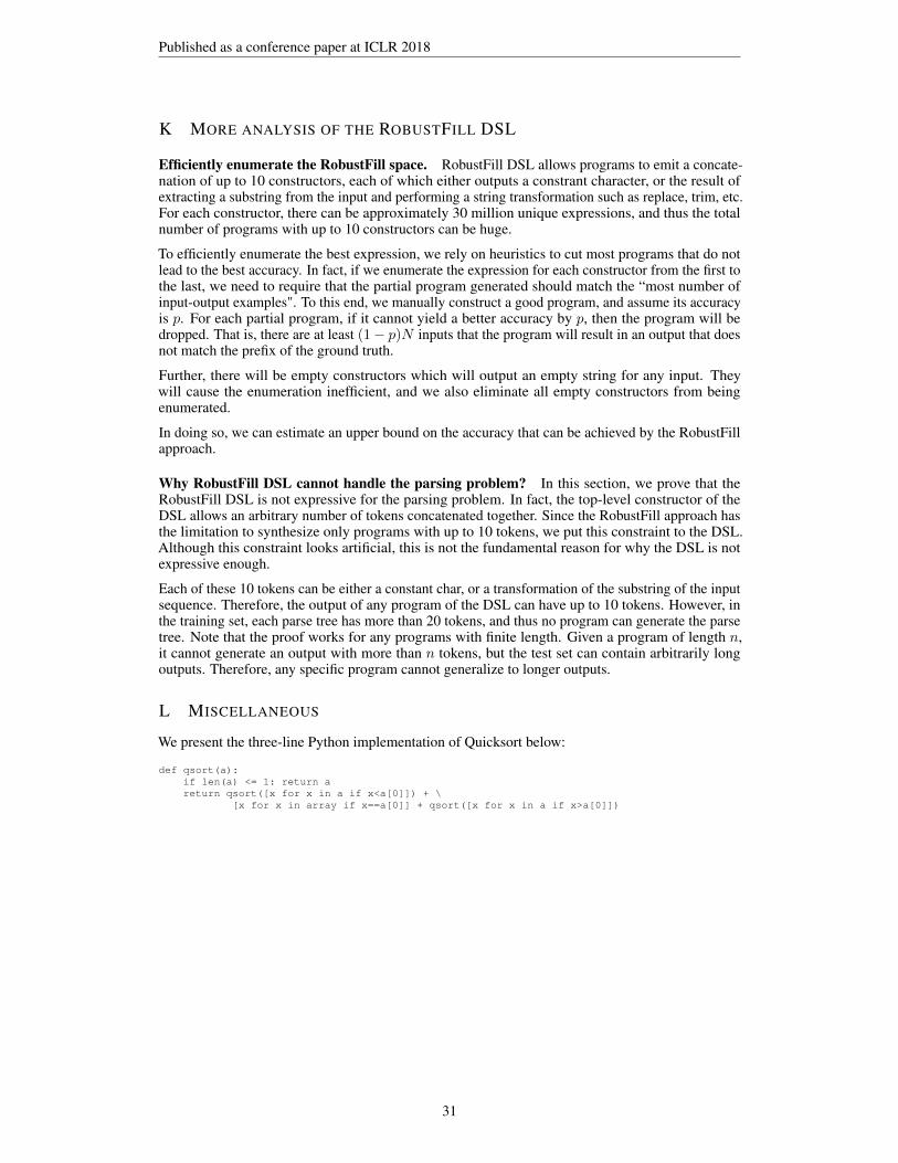
Published as a conference paper at ICLR 2018
K MORE ANALYSIS OF THE ROBUSTFILL DSL
Efficiently enumerate the RobustFill space. RobustFill DSL allows programs to emit a concate-nation of up to 10 constructors, each of which either outputs a constrant character, or the result ofextracting a substring from the input and performing a string transformation such as replace, trim, etc.For each constructor, there can be approximately 30 million unique expressions, and thus the totalnumber of programs with up to 10 constructors can be huge.
To efficiently enumerate the best expression, we rely on heuristics to cut most programs that do notlead to the best accuracy. In fact, if we enumerate the expression for each constructor from the first tothe last, we need to require that the partial program generated should match the “most number ofinput-output examples". To this end, we manually construct a good program, and assume its accuracyis p. For each partial program, if it cannot yield a better accuracy by p, then the program will bedropped. That is, there are at least (1− p)N inputs that the program will result in an output that doesnot match the prefix of the ground truth.
Further, there will be empty constructors which will output an empty string for any input. Theywill cause the enumeration inefficient, and we also eliminate all empty constructors from beingenumerated.
In doing so, we can estimate an upper bound on the accuracy that can be achieved by the RobustFillapproach.
Why RobustFill DSL cannot handle the parsing problem? In this section, we prove that theRobustFill DSL is not expressive for the parsing problem. In fact, the top-level constructor of theDSL allows an arbitrary number of tokens concatenated together. Since the RobustFill approach hasthe limitation to synthesize only programs with up to 10 tokens, we put this constraint to the DSL.Although this constraint looks artificial, this is not the fundamental reason for why the DSL is notexpressive enough.
Each of these 10 tokens can be either a constant char, or a transformation of the substring of the inputsequence. Therefore, the output of any program of the DSL can have up to 10 tokens. However, inthe training set, each parse tree has more than 20 tokens, and thus no program can generate the parsetree. Note that the proof works for any programs with finite length. Given a program of length n,it cannot generate an output with more than n tokens, but the test set can contain arbitrarily longoutputs. Therefore, any specific program cannot generalize to longer outputs.
L MISCELLANEOUS
We present the three-line Python implementation of Quicksort below:
def qsort(a):if len(a) <= 1: return areturn qsort([x for x in a if x<a[0]]) + \
[x for x in array if x==a[0]] + qsort([x for x in a if x>a[0]])
31