Systolic convolution of arithmetic functions · Systolic convolution of arithmetic functions 209 2....

Theoretical Computer Science 95 (1992) 207-229

Elsevier

207

Systolic convolution of arithmetic functions *

Patrice Quinton IRISA, Campus de Beaulieu, 35042 Rennes Cedex. France

Yves Robert LIP-IMAGI Ecok Norm& Sup&ieure de Lyon, 46 ai& d’Italie, 69364 Lyon Cedex 01, France

Communicated by D. Perrin

Received January 1989

Revised March 1990

Abstract

Quinton, P., and Y. Robert, Systolic convolution of arithmetic functions, Theoretical Computer

Science 95 (1992) 207-229.

Given two arithmetic functions J and g. their convolution h=f* q is defined as h(n)=

Lr=.. 1 Bk,, 4n f(k) g(l) for all n> 1. Given two arithmetic functions g and h, the inverse convolution problem is IO determine J such that f* g = h.

In this paper, we propose two linear arrays for the real-time computation of the convolution and

the inverse convolution problem. These arrays extend the design of Verhoeff for the computation of

the Miibius function p, defined as the solution of the inverse convolution problem p *g = d, where

g(n)= 1 for all n> I and d(n)= 1 if n= 1, d(n)=0 if n> 1.

1. Introduction

Given two arithmetic functions f and g, their convolution h=f * g is defined as

h(n)=k=,, lSk,.lbn f(k) g( 1) for all n 2 1. Given two arithmetic functions g and h, the

inverse convolution problem is to determine f such that f * g = h. The inverse convolu-

tion problem is not always solvable; see [S] for a review.

For instance, let Eo(n)= 1 for all n>, 1 and d(n)= 1 if n= 1, d(n)=0 if y1> 1. The

Miibius function lu is defined as

An)= 1 if n= 1,

*This work has been supported by the Research Program C3 of the French National Council for Research CNRS and by the ESPRIT Basic Research Action 3280 of the European Economic Community.

0304-3975/92/$05.00 c 1992-Elsevier Science Publishers B.V. All rights reserved

208 P. Quinton. Y. Roherl

P(n)=(- I)* if H is the product of r distinct primes,

An)=0 if n is divisible by a prime square.

din denotes that d is a divisor of n. The Mobius function can be more easily computed

using the Mobius inversion formula [S]

c Ad)=d(n),

which states that ,u is the solution to the inverse convolution problem ,u * E,, = d.

Verhoeff [16] proposes a systolic linear array for the real-time computation of the

Mobius function p. In this paper, we propose two systolic architectures for the

real-time computation of the convolution and the inverse convolution of general

arithmetic functions. Kung [6] introduces a systolic linear array for the computation

of the sequence

h(n)= c .f(k)g(l), n3 1, k+l=n+l,lSk.l<n

where (f(k); k 3 1) and (g( 1); 13 1) are two given sequences. Such a computation

corresponds to the product of two polynomials, or series, with coefficientsf(k) and

g(l). Informally, if we want to compute h(n) = I,, Jf( d), we can use a design similar to

that of [6]. The problem is to inhibit the operation of the cells when they receive a pair

of inputs (f(d), h(n)), where d is not a divisor of n, and this is the key to Verhoeff’s

design [ 163.

The general convolution problem h =f* g is more difficult for two reasons:

l First we have to ensure that every component off can meet every component of g.

l When a cell receives a pair of inputs (f(d), h(n)), where d is not a divisor of n, its

operation has still to be inhibited. But when d is a divisor of n, we have to organize

the flow of y such that g(n/d) is also an input to the cell.

In this paper, we first propose a linear systolic architecture of O(N) cells which

solves the problem of computing (h(n); 1 <n < N) in time O(N). This first solution is

obtained using the dependence mapping method. The space-time complexity of the

proposed architecture is 0( N2 log N). Then we propose another systolic architecture

of only O(N ‘I’) processing cells which also solves the problem in time O(N). This

second architecture requires 0( N log N) delay cells, leading to the same space-time

complexity as for the first solution. Both architectures can be extended to the solution

of the inverse convolution problem, with the same performances.

Throughout the paper, we assume the reader to be familiar with the systolic model.

Systolic arrays have been introduced by Kung and Leiserson [S] and consist of a large

number of elementary processors (or cells), which are mesh-interconnected in a regu-

lar and modular way, and achieve high performance through extensive concurrent

and pipeline use of the cells. We refer the reader to [7] for a general presentation of the

systolic model.

Systolic convolution of arithmetic functions 209

2. A first linear systolic array

The arithmetic convolution consists in the computation of the following equation:

wheref( k), k> 1 and g(l), / > 1 are given integer functions.

Let K be a fixed parameter. Systolic arrays that compute the convolution

v’n>l, h(n)= 1 .f(k)g(n--k+l) 1 Qk<X

are well known (see, for example, [7]). From the bidirectional design of Kung, one can

easily derive a systolic array for the unbounded convolution, i.e. the convolution whose

equation is

v’n 3 1, h(n)= c ,f(k)g(n--k+ 1). (3) 1SkQn

The only difficulty is the loading of the coefficients g, as one cannot assume that

they are preloaded in the array, as in the case of the bounded convolution.

The arithmetic convolution (1) is much harder, as the summation has only to be

done for product terms f(k) g(l) such that kl =n.

In what follows, we derive and prove the correctness of a systolic array which has

the following characteristics:

l The array is linear and bidirectional. The number of cells needed for the computa-

tion of h(n), 1 d n 6 N, is N.

l The period of the array is 3, i.e. each cell works every three cycles.

We shall derive the design using a space-time transformation of a dependence

graph of the algorithm, following the approach of Moldovan [lo] and Quinton [ 111.

In Section 2.1, we recall the principles of the dependence mapping method on the

example of the unbounded convolution. In particular, we explain how the coefficients

g(I) can be loaded in the cells. In Section 2.2, we develop the arithmetic convolution.

2.1. Unbounded convolution

Figure 1 depicts a dependence graph for the unbounded convolution. For the

moment, we ignore the loading of the g coefficients. On this diagram, a coefficient h(n)

is computed along a diagonal line, by summing up the product terms f‘(k) g( n - k + 1)

in increasing order of k. The result h(n) is obtained at point (n, 1). Deriving a systolic

array from this dependence graph can be done easily using a space-time linear

transformation (see [ 10, 1 l] among others). First we seek an affine (integral) schedule

of the computations, i.e. a function t(n, m) such that if calculation at point (n,, ml)

depends on calculation at point (n2,m2), then t(n,,m,)>t(nz,m2). Denote

t( n, m) = A1 n + jL2 m + a, where Ai, I., , and M belong to Z, the set of integers. Let us call

dependence vector the quantity (nl -n2, ml -m2) for two dependent points. As the

210 P. Quinton, Y. Robert

n

Fig. I. Dependence graph and timing function for the convolution.

number of dependence vectors in this graph is finite (and independent of n), this

condition amounts to a finite number of linear inequalities involving these vectors.

The set of possible dependence vectors is

A={(02 l),(l, -l),(l,O)}

We must, therefore, have

ix> 1; j_r-i,> 1; /1131.

These conditions are met optimally with ;1r = 2 and I., = 1. The coefficient x can be

chosen in such a way that the computation starts at time 0 by taking c( = 3. Thus, an

optimal timing-function is t (n, m) = 2n + m - 3.

A well-known systolic array can be obtained by projecting the array along the

n axis. Figure 2 shows this systolic array which uses N bidirectionally connected cells,

for the computation of h(n), 1 <n d N. The detail of the cells is shown in Fig. 3, where

s is a boolean control signal.

Coefficients h(k) are computed when they flow from the right to the left, and output

by the leftmost cell. Note that the period of the array is 2, and this can be clearly seen

on the dependence graph.

In this first design, coefficient y(I) is pre-loaded in cell 1. The best way to solve this

problem is to fold the dependence graph along the bisectrix of the first orthant, in

order to let f’ and g play a symmetric role with regard to the projection direction.

However, to do so, it is first necessary to change slightly the way the h coefficient is


Fig. 2. Systolic array for the usual convolution.

: rjijEh h*~-E

time t time t+l

f’ :=“f; S’ :=s;

case S + h’:=f.g; (first computation)

nots + h’:=h+f,g; {update}

esac

Fig. 3. Operation of the cells for the unbounded convolution.

summed up, so that the direction of its movement remains the same once the domain

is folded. The trick is to compute the summation starting by the middle, as shown in

Fig. 4.

In the new dependence graph, g(l) and f( 1) flow together, starting from point n = I,

m = 1, and are reflected along the line n = m. Therefore, h(p), moving along the straight

line n+m=p+ 1, meets successively the pairs (g(l),f(l)) and (g(p--I+ l),f(p-I+ l)),

when 1 ranges from Lp/2] down to 1.

By projecting the dependence graph along the n axis, one obtains the systolic array

depicted by Fig. 5, whose cells are shown in Fig. 6.

h

Ill

t

f(1) f(2) f(3) f(4) f(5) f(6) f(7) f(8)

cl(l) g(2) 90) g(4) g(5) cl(G) g(7) g(8)

n

Fig. 4. Dependence graph and timing after folding

212 P. Quinron, Y. Robert

h

fl 4 0 n-0 III

g1’l=._(I_cl

controC--+

Cell 0 Cell 1 Cell 2 Cell 3

Fig. 5. Systolic array for the unbounded convolution.

1’21 h fl

gl TE El

contra

time t time t case

c~mtrol= initodd+ (this case for the points on line n=m I begin

.j2 :=./‘I; 92 :=gf; (load,fI and yl in registers) h’:=,f7 *y2: (compute middle term of the sum}

end control = inilerw + (this case for the points on line n = 111 + 11 begin

.f’1:=.1’/; q’I:=gf; (transmitf7 and 81) h’:=ff*yZ+f_7*yl; (compute middle term of the sum}

end

otherwise+ (normal case j begin

,f’I:=.fl;~‘I:=ql; (transmit ,j’f and yl)

h ’ := h +.1‘1 * (, I +,l2 * </2; ( update with next term of the sum) end

esac confrol’:= control; (transmit control )

Fig. 6. Detail of the cells of the systolic array for the unbounded convolution,

A few words of explanation about the control of the cells are in order. As shown

in Fig. 4, depending on the parity of p, h(p) starts its computation at the point

((p+ 1)/2, (p+ 1)/2) when p is odd, or at (p/2+ 1, p/2) when p is even. Moreover, the

pair of coefficients g,.f is reflected on point ((p + 1)/2, (p + 1)/2). These peculiarities of

the operation of the cell are taken care of by introducing a signal named control which

can take the value initodd, initecen or normal. When control = initodd, the coefficients

,f and g are loaded in the registers, and h is initialized with the value .f* g. When


control = i&even, h is initialized withf 1 * g2 +f2 * gl. Finally, in the normal case, h is

incremented withf 1 * g2 +f2 * gl. The signal control flows along the direction given

by vector (1, 1) on Fig. 4. Therefore, it visits a new cell every three cycles. Along the

diagonal n = m, control = initodd. Along the line n = m + 1, control = initeven. Other-

wise, control = normal.

2.2. Arithmetic convolution

The problem is to compute the convolution h =f * g. For all n 3 1, we need to

evaluate the sum h(n)=C,,=n,1Qk,16n f(k) g(1). The constraints are the following:

l Communications with the host: there is only one cell in the array communicating

with the host. This cell receives the input sequences (f(n); n 3 1) and (g(n); II 3 1)

and delivers the output sequence (h(n); n3 1).

l Real-time computation: for all n3 1, h(n) should be output by the array k units of

time after the input of f(n) and g(n), where k is a fixed constant independent of n, l Modularity: the operation of the cells should not depend upon their location in the

array, nor should it depend on the indices of their inputs/outputs. Provided that

this condition is met, the array can be used for the computation of an arithmetic

convolution of any size.

Figure 7 shows a dependence graph for the arithmetic convolution. As in the usual

convolution, coefficient h(p) is computed along the diagonal line, whose equation is

n + m = p + 1. The problem is to “route” the coefficients g and f used for computing the

product terms, in such a way that the graph be uniform and that these coefficients

meet on the right line. The choice that is made here consists in routing the coefficients

g and f in a symmetric way, so that g(n) and f(n) meet on the first bisectrix. For

example, g(2) and f(2) meet at point (S/2,5/2), just on the line where h(4) is summed

up, and coefficients g(3) and j”(3) at point (5, 5), which is just on the line m= 10-n

where h(9) is computed. The diagram shows intuitively that when the g’s and thef’s

flow on straight lines, they meet on and only on the lines where they are used. This is

confirmed by the following obvious lemma.

Lemma 2.1. Consider the family of points

.)(1+1)/2+1,(1-l)(k+1)/2+1), X(k, l)=(G(k), F,(O)=((k- 1

where k>l and 131.

Then the curves {X(k,l)jkSI and {X(k, on the line m=kl+ 1 -n.

l)}Ia 1 are straight lines. Moreover, they meet

Lemma 2.1 clearly states that the routing scheme shown in Fig. 7 is correct.

However, as it is, this dependence graph cannot be used for deriving a systolic array,

for three reasons:

(1) the underlying lattice of the graph is not integral;

(2) there exists an unbounded number of dependence vectors;


Fig. 7. Dependence graph for the arithmetic convolution.

(3) we must provide a mechanism to avoid pre-loading of the g coefficients.

Problem 1 can be solved by a dilation of the graph by 2 along both directions. We

shall also solve problem 3 by applying the same trick as for the unbounded convolu-

tion, i.e. by folding the dependence graph.

Problem 2 is more involved. The solution consists in replacing the straight lines

where the coefficients g and f flow by a piecewise linear curve that meets the following

conditions:

(a) the curve follows a finite number of directions;

(b) all the intersection points are on the curve;

(c) the number of curves passing through a given point of the plane is bounded.

Condition (a) is necessary if one wants to obtain a finite number of dependence

vectors. Condition (b) is obviously necessary to keep the properties of the previous

dependence graph. Finally, condition (c) is needed for the resulting systolic array to

have only a finite amount of data to be transmitted from one cell to another. This last

condition is the reason why we have chosen the symmetric routing scheme (other

simpler routing schemes are possible; for example, to havef( k) flow on line n = k and

route g(l) to the point (k, kl+ l), but in this case, condition (c) could not be met).

Let us first ignore the problem of loading the g coefficients. Figure 8 shows the

dependence graph after dilation by 2 along both axes (in order for the intersection


Fig. 8. Piecewise approximation of 9 and f movement

points to be on an integral lattice), once the straight lines are replaced by a piecewise

approximation. This approximation can be explained as follows.

Let {G/(k, i)}k3i,0<i<l+i be the curve, parameterized by k and i, defined by

((k-1)(/+ l)+i+2, (1- l)(k+ 1)+2) if Odi<2, G;(k, i)=

((k-l)(l+ 1)+4, (1- l)(k+ l)+i) if 2<i<l+ 1.

Informally, the points of this curve are obtained by starting at point (2,21), and

moving once along vector (2,O) and then l- 1 times along vector (1, 1).

Similarly, let {F;(I, i)}[ai,l)$i<k+i be the curve, parameterized by I and i, defined

by

1

((k- 1)(1+ l)+i+2, (l-l)(k+ 1)+2) if Obi<2, Fi(1, i)=

((k-1)(1+1)+4,(1_l)(k+l)+i) if 2<i<k+ 1.

The following lemma proves that the piecewise approximation meets the previously

stated conditions.

Lemma 2.2. For all 1, k30,

(1) (G;(k, i)}kzl,0<i<l+l, (F;(I, i)}lal,0<i<k+l, and the straight line n+m=

2( kl+ 1) are concurrent,

(2) The family of curves { G;(k, i)} ({ F;(l, i)}) has no intersection point.

Proof. (1) is easily seen, as G;(k,O)=F;(/,O)=((k-1)(1+1)+2,(1-l)(k+1)+2),

which is just twice the coordinates of the point X that we have already seen in Lemma

2.1. The proof of (2) is also very simple. 0

216 P. Quinton, Y. Rohrrt

The loading of the y coefficients is solved in a similar way as already seen in the

unbounded convolution, i.e. by folding the dependence graph along the line n = m. The

resulting dependence graph is shown in Fig. 9. The pairs (f(n), g(n)) are input along

the n axis, and are reflected when they meet the line n = m. The dependence vectors are

also shown in Fig. 9. They are

Therefore, the parameters i1 and 3., of the timing function must satisfy

2j”23 1, 11+A221,

2i,31, i.1 -3.12 1.

The optimal (rational) solution is i1 = 3/2 and AZ= l/2, which gives the timing

function t( n, m) = L 3n/2 + m/2 - 4 J, as shown in Fig. 9 (the interested reader is referred

to [I 11 for the use of rational timing functions).

The final architecture (Fig. 10) is obtained by projecting the dependence graph

along n axis. We can immediately see that the number of cells needed for computing

Dependence vectors

Fig. 9. Final dependence graph for the arithmetic convolution.

Systolic concolution qf arithmetic functions 211

init

h

cell 1 cell 2 cell 3 cell 4

Fig. 10. Systolic array for the arithmetic convolution

the sequence h(k), 1 d kdn is n. Each cell of the array works only every three cycles.

Each cell except for the first one has four left-to-right, and one right-to-left links: _ init carries a initialization signal which follows the line n=m on the dependence

graph of Fig. 9. This signal reaches a new cell every other time;

- fast carries the f and g coefficients moving along direction (0,2) on Fig. 9, as well as

other informations that will be detailed later on. After being processed by a cell,

these values skip the next cell and reach the second next one;

~ slow1 and slow2 carry two pairs off and g coefficients (as well as other informa-

tions) moving along direction (1, 1);

~ h carries the value of the h coefficient under computation.

Finally, each cell is provided with a register R which keeps the pair f and g flowing

along the direction (2,0) in Fig. 9: this direction being projected in the same cell, it

corresponds to the storage of a value in one cell. The first cell is special. It has only

a slowl, an h and an init link.

The details of the operation of the cells are shown in Fig. 11. Actually, each one of

the fast, slow1 and slow2 link carries a 5tuple (f, g, valid, rank, count), where f and

g are coefficients, valid is a boolean indicating that the link effectively carries signifi-

cant values, rank is the number of the coefficients, and count is an integer which will be

used to determine the movement of the pair J g. To understand the operation of the

cell, it is best to refer again to the dependence graph of Fig. 9. As already seen, a pair

(f(k), g(k)) moves once along the direction (0,2) and then k times along the direction

(1, 1). After the pair is reflected along the line n = m, it moves once along the direction

(2,O) and k times along the direction (l,l). The rank parameter is used to remember

the k value, and count is decreased when doing the k movements along the direction

(1, 1). When count reaches 0, then two pairs of coefficients are available on slow1 and

slow2 and the h coefficient is modified.

2.3. Perfbrmances

In fact, although each cell is activated every three cycles, the actual efficiency of the

network is less than l/3, as the number of calculations to be done (in sequential) for


init init

fast

time t time t+l

case

init and slowl.count#O~ (initialization and no calculation)

begin h’:=O; init’:=init end;

init and slowI.counr =O+ (initialization and calculation) begin

/I ‘:= /I + slow1 .,f* slowl .y; R := slow1 {store slowI in R); inir’:=init

end;

not init andfust.calid+ (send,fhst on slowl, reset count)

begin

slowl’:=,firs~; slowI’.~ount:=runk- 1; init’:=inir; h’:=h

end;

not init and slowl. calid and slowl .count #O and R. valid+

begin {send R on ~10~2, decrease count of slowl ) .~lowl’:=sl0wf,~ sloal’.counr :=slowl’.count- 1;

s10).\2’:= R; R.aulid:=jiilse; init’:= inir; h’:= h

end;

not init and slw I. rulid and slo\vI. count # 0 and not R. valid+

begin [keep values moving on slow lines, decrease count of slowl)

.slowI’:=slo~~~I; siu~~I’.cuunt:=~lo~~~I’.c~~nr-1;

slow2’:=slo~v2; init’:=inir: h’:=h

end:

not init and slowf. oulid and slowf .cmnt =O+

[note that slow2 is necessarily valid ]

begin {compute. send .slowl on fusr and keep slow2 in R}

h’:=h+slowf.J*slow2.y+.slow2.,f*slowl.~;

R:=slo~~2;,fust’:=slo~l; init’:=inir

end

esac

Fig. 11. Operation of cell i, i > 2

computing h(n) is not of the order of n: computing (h(n); 1 < n 6 N) requires

1 div( n) = 0( N log N) multiplications, 1 Qfl<N

where div(n) is the number of divisors of n.

In summary, this first solution uses O(N) cells for processing in time O(N) the

computation of the sequence h(n), 1~ n < N. However, as each cell n has to make use

of a counter initialized to n, the area complexity of this design is 0( N log N).

Systolic convolution ofarithmetic functions 219

init

slow

-4

1 z h h’

init’

fast’

time t time t+l

case init+ {initialization: compute and store in R} begin

h’:=slowl.f*slowl.g; R:=slowl; {store in R} init’ := init

end; not init+ (first cell, normal case}

begin h’:=h+slowl.f*R.g+R.f* slow1.g; R:=R {store in R}; init’:=init

end; esac

Fig. 11 (continued). Operation of the first cell.

3. Another systolic design

In this section, we design another systolic array of processors for the parallel

computation of the convolution of two arithmetic functions. We address the inverse

convolution problem in Section 3.4. The second array will look like the one shown in

Fig. 12.

3.1. Half computation

First, we show how to compute the sum h,(n) = 1 kl = n, k > J( k) g(I). The other half

of the arithmetic convolution will be computed similarly. We use a linear array of

cells, as in Fig. 12, and number the cells from left to right.

l Input and output (Z/O) format. For all n3 1, f(n) and g(n) enter the array at time

n; Al(n) is output at time n (see Fig. 13).

(h(n); nrl) t- (g(n); n21) +b

e- e- e- +

+ + + . . .

(f(n); =-I) --p + + + __)

Mast ; cell 1 cell 2 cell 3 cell4

Fig. 12. The second linear array.

220 P. Quinton. Y. Robert

h,(l) h,(2) h,(3)

,,, ;;; g; w; w; “,‘:; gyjyL=zJ.. cell 1 cell 2 cell 3

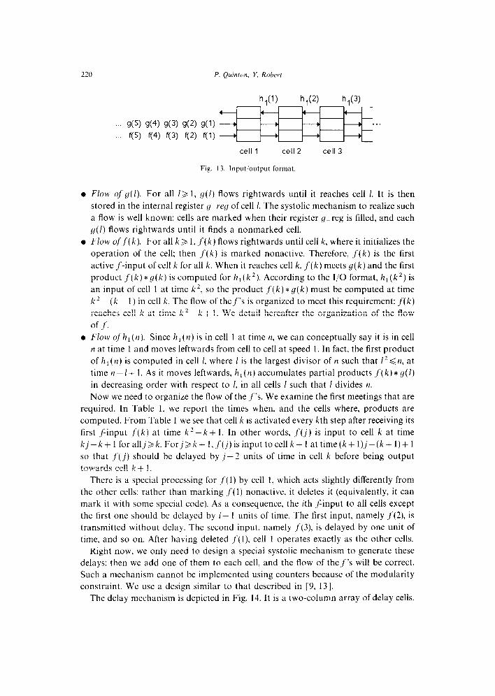
Fig. 13. Input/output format.

Flow, of’g(1). For all /> 1, g(I) flows rightwards until it reaches cell 1. It is then

stored in the internal register y_rey of cell 1. The systolic mechanism to realize such

a flow is well known: cells are marked when their register g_reg is filled, and each

g(l) flows rightwards until it finds a nonmarked cell.

Flow of,f( k). For all k 3 1, ,f( k) flows rightwards until cell k, where it initializes the

operation of the cell; then f(k) is marked nonactive. Therefore, f(k) is the first

active f-input of cell k for all k. When it reaches cell k, f(k) meets g(k) and the first

product J(k)*g(k) is computed for hl(k2). According to the I/O format, hl(k2) is

an input of cell 1 at time k2, so the product f(k) * g(k) must be computed at time

k * - (k - 1) in cell k. The flow of thef”s is organized to meet this requirement: f(k)

reaches cell k at time k * -k + 1. We detail hereafter the organization of the flow

of f’.

Flotv qfhl (n). Since k,(n) is in cell 1 at time IZ, we can conceptually say it is in cell

n at time 1 and moves leftwards from cell to cell at speed 1. In fact, the first product

of h 1 (n) is computed in cell I, where 1 is the largest divisor of n such that 1’ d n, at

time II - I+ 1. As it moves leftwards, h, ( II) accumulates partial products f(k) * g( 1)

in decreasing order with respect to 1, in all cells 1 such that 1 divides n. Now we need to organize the flow of the .f”s. We examine the first meetings that are

required. In Table 1, we report the times when, and the cells where, products are

computed. From Table 1 we see that cell k is activated every kth step after receiving its

first ,f-input f(k) at time k* - k + 1. In other words, .f(j) is input to cell k at time

kj-k+1forallj~k.Forj~k+l,f(j)isinputtocellk+lattime(k+l)j-(k+1)+1

so that f(j) should be delayed by j-2 units of time in cell k before being output

towards cell k + 1.

There is a special processing for f(l) by cell 1, which acts slightly differently from

the other cells: rather than marking ,1‘(l) nonactive, it deletes it (equivalently, it can

mark it with some special code). As a consequence, the ith ,f-input to all cells except

the first one should be delayed by i- 1 units of time. The first input, namely f(2), is

transmitted without delay. The second input, namely J(3), is delayed by one unit of

time, and so on. After having deleted j’(l), cell 1 operates exactly as the other cells.

Right now, we only need to design a special systolic mechanism to generate these

delays: then we add one of them to each cell, and the flow of thef’s will be correct.

Such a mechanism cannot be implemented using counters because of the modularity

constraint. We use a design similar to that described in [9, 131.

The delay mechanism is depicted in Fig. 14. It is a two-column array of delay cells.


Table 1

Space-time diagram for the computation of partial products

Times Cell 1 Cell 2 Cell 3 Cell 4 Cell 5

1

2

3

4

5

6

7

8

9

10

11

12

13

14

15

16

17

18

19

20

21

f (4 m

f (3) m

.f(4). da

f(5). g(2)

f (6). g(2)

f(7). s(2)

f (8). .d2)

f (9) g(2)

f(lO).d2)

fUl).d2)

f (3). s(3)

f(4) g(3)

f (5). Y(3) f (4 Y(4)

.f(6). g(3) f (5) g(4)

f (7) Y(3)

f (6) ~(4) f (5) Y(5)

The first column is composed of cells with one input and three outputs. The operation

of the cells in the first column is very simple (Fig. 15):

l the first input is output rightwards on the fast channel;

l the second input is output rightwards on the slow channel;

l all following inputs are output downwards to the next cell in the column.

The cells of the second column simply transmit their valid input, if any (to

implement this, they perform an OR-operation on their two inputs, where non-

specified variables have the default value nil). Some consecutive time-steps of the

mechanism are illustrated in Fig. 16.

Fig. 14. Delay mechanism.


fw

E ___

Time t= 0

a3 b3

skat s&Q t+1

case status of

.first: begin b, :=a,; status:=second; end

second: begin b, := a, ; stutus := marked; end

marked: begin h, := a, ; end

b, :=a2 OR a,;

Fig. 15. Operation of the delay mechanism

_-.

Time t= 1

r-(4)

Y4) ft3)

88 ___

Timet= 2

f(3)

ft5)

Y4)

88 ___

Time t= 3

ft5)

.-. . . . . . . . . .

Timet=4 Time t= 5 Time t= 6 Time t= 7

Fig. 16. Some consecutive time-steps for the delay mechanism

The full operation of the cells for the computation k, (n)=Ckl=n,k~If(k)~(I) is

described in Fig. 17, where nonspecified variables have the default value nil. As stated

above, the operation of cell 1 is slightly different since its first input is deleted.

Proof of correctness

We know that f(k), k > 1, reaches cell 1 at time kf + k - 1. If k 3 1, f(k) is active in cell

I, and the product f(k) * y( 1) is computed. Consider the computation of k, (n): k,(n) is


bout

gin

aCtivein)

bin

gout

(foutj activeout )

. . .

(store gin in g_rey if nonmarked}

if nonmarked then

hegin g_reg := gl.; nonmarked :=false; end

else go”, := g,.; {active f-input }

if active,, then

begin

{inactivate first f-input} ifjrst_f then begin actioe,,:=false; first_/ :=false; end

{update hi,} h,,, := hi, + g-reg *f,.;

end

{delay all f-inputs}

(fO”,> actice,,,):= DelayPMechanism (J., actils,);

Fig. 17. Operation of the cells of the array.

h

.-. _.. mm_

Fig. 18. Systolic array for the arithmetic convolution h =f * g,


(4’jnj active’in)

“in

bout

9 in

(fin, activein)

(g’,utJ active&)

LJt

bin

gout

u out 1 activeout)

{store gi. in y-q and& in f_reg if nonmarked}

if nonmarked then begin y_reg := yin; f_ reg :=f;b; nonmurked :=,false; end

else begin you, := qr”; j&, :=./;A; end

{active ,f-input and g’-input. Note that activei, = actice;, by symmetry)

if actice,, then begin

[inactivatef- and y’-inputs}

if f;rst_fg’ then begin active,, :=,false; actire:, :=false; first-jg’ :=false; end

{update h,,)

h,,,:=k,.+g~r~g*.1;,+f_reg*gr,;

end {delay all 1’ and g’-inputs)

(“/A, actice,,,) := Delay-Mechanism (A., active,,):

(gL,,, actire&,) := Delay-Mechanism (g;,, active:.);

Fig. 19. Operation of the cells for the arithmetic convolution h =j’* g.

in cell I at time n-l+ 1. It meets some f(k) there if and only if U--I+ 1 =n-l+ 1, i.e.

kl= n. Then h, (n) is updated into hI (n):= hl (n) +f( k)g( I) if and only if f( k) is active

or, equivalently, k>l. Therefore, the final value of h,(n) is hl(n)=~~,,n,,~,f(k)g(l) as expected.

3.2. Systolic arithmetic convolution

For computing ~(~)=~,,&‘(k)g(4, we use two copies of the previous array. In the

first array, we compute hl(n)=~:,,,,,,~,f(k)g(l) as before.

In the second array, we compute h2(n)=xkl=n,k,l g(k)f(l). We interchange the

Bows off and g in the second array: the f’s are stored in the cells, and the g’s move

Sptolic convolution of arithmetic firnctions 225

rightwards with delays. The only modification is that the second array should not

compute products j(k) *g(k), as they are already computed by the first array. We

simply modify the operation of the cells (except the first one) as follows: the first time

they receive an active g-input, they let h,(k’):=O rather than h,(k2):=f(k)* g(k). In

fact, we can make things simpler by coalescing the corresponding cells of both arrays,

as described in Fig. 18. Again, the first cell is slightly different because it deletes its first

f-input (bottom part) and its first g-input (top part). Also, it duplicates f- and

g-inputs. See Fig. 19 for the operation of all cells but the first one, and Fig. 20 for the

operation of the first cell.

gin

fin

‘out

bin

gout

(rout I activeout)

if nonmarked then begin

{yx. =g( 1);1;, =.f( 1); store and mark cell}

J_reg :=J,; y_rey:=yi,; nonmarked:=false;

{delete fou, and y&,1 fI,, := nil; y&, := nil;

{compute h(l)) h,,, :=fin*yln; end

else begin

{transmit gin and .G I CL,, := g,.; .!A :=.fi,; {update h,,} h,,, := hi. +y-rey*j;” +f-rey*y;,;

{activatef-input and g’-input 1 actiue,, := true; active,‘, := true;

{delay alIS_ and y’-inputs}

CL,> active,,,) := De/a~_Mechanism(f;,, activei,);

(yl,.,, actioeA.,) :=Delay~Mrchanism(gl,. acti&); end

Fig. 20. Operation of first cell for the arithmetic convolution h=f* g.


3.3. Performances

For the computation of (h(n); 1 dn < N), we have designed an array of N”’

processing cells (which perform multiply-and-adds). Note that the total number of

delays is proportional to N log N, and not to N, although we have only O(N) inputs.

To see this, consider for instance the first array. The last element that we need to

consider in cell k is .f( N/k), to be multiplied by g(k). f( N/k) has been delayed by N/k units of time in cells 1,2,. . , , k - 1 before reaching cell k. So that we need N/2 delays in

cell 1 (due to f( N/2)), N/3 delays in cell 2 (due to f( N/3)), N/4 delays in cell 3 (due to

f(N/4)), and so on up to N/N ‘I2 delays in the cell before the last one (due to f(N”‘)).

3.4. The inverse arithmetic convolution problem

The previous array can be very easily modified to solve the inverse arithmetic

problem. This is quite similar to the technique used for moving from FIR filtering to

IIR filtering [7] or from polynomial multiplication to polynomial division [6].

To compute (whenever possible) the function f such that f* g = h, we observe that

.f(l)=h(l)ltr(l)>

.f(n)= h(n)- 1

c f(k)g(l) kl=n. l<k.l6n,k#n Ii g(1) if n> 1.

We input to the array the sequence (g(n); n3 1) in the same format as before. We

replace the input sequence (j”(n); n> 1) by the sequence (h(n); nB l), with the same

format (Fig. 21). All cells operate exactly as before, except the first one whose program

is given in Fig. 22.

. . . . . . . . .

. f-r- out

. I

’ h-sum I

g-v 4 g_w --* g-w + g

h:_

___ ___ .._

Fig. 21. Systolic array for the inverse arithmetic convolution problem.


gin

f-res,ut

bin

(9’ out, active’out)

fbut

h_sumin

gout

(f out I activeout)

if nonmarked then

begin

{yi,=y(l); h,,=h(l); computef_res,,,=f(l)} f_res,,, :=hi,/gi,; {store and mark cell} f_reg:=f_res,,,; g-reg := gin; nonmarked :=false;

{delete fOu, and g:.,} fOut := nil ; g&, := nil;

end

else

begin

{compute f-res,,,} f-i-es,,, := (hi,- h-sum,.-f_reg*gi.)/gpreg; {transmit gi. and f,b} g.., := gin; fd,, :=f_res& {activate f-input and g’-input} activei,:= true; active:, := true; {delay all f- and g’-inputs}

CL.,> actioe,,,) :=Delay_Mechanism( f_res,,,, active,,);

(i.,, active;.,) := Delay_Mechanism(gj., active:,); end

Fig. 22. Program of first cell for the inverse convolution problem.

The performances are the same as for the direct arithmetic convolution. We use

N ‘1’ processing cells and 0( N log N) delays for the computation of the sequence

(f(n); 1 ~nb N) with N units of time.

4. Conclusion

We have presented two linear systolic arrays for the real-time solution of the

arithmetic convolution and of the inverse arithmetic convolution problem. Both


arrays extend Verhoeff ‘s design for the Mobius function to solve the general arith-

metic convolution problem. Our first design is a linear array of O(N) cells that solves

the problem in time O(N), thereby delivering the same performances as Verhoeff ‘s

design. Our second design requires only O(N “‘) computational cells. We believe it

would be an interesting challenge to derive this second design completely automati-

cally, using the synthesis methods of [l, 3, 10, 1 l] or the parallel constructs of [15, 161.

Acknowledgments

The authors thank Tom Verhoeff for bringing the arithmetic convolution problem

to their attention during a workshop organized by Alain Martin in La Jolla, Califor-

nia, USA, on February 22-26, 1988. Tom Verhoeff presented its design for the Mobius

function [16] and raised the problem of systolizing the general arithmetic convolu-

tion. We designed the first solution (reported in this paper see also [12]) two months

after the workshop. At the time of this writing, we are aware of three other solutions,

by Chen and Choo [a], by Duprat [4] and by Struik [14]. These three solutions are

variations on the first design presented in this paper, in that they are linear arrays of

O(N) cells that solve the arithmetic computation problem in time O(N).

References

[1] M. Chen, Synthesizing VLSI architectures: dynamic programming solver, in: K. Hwang et al., eds.,

Proc. 1986 Inter-nut. Conf: on Parallel Processiny (IEEE Computer Sot. Press, Silver Spring, MD,

1986) 7766784.

127 M. Chen and Y. Choo, Synthesis of a systolic Dirichlet product using nonlinear contraction domain,

in: M. Coward et al., eds., Purallel and Distributed Algorithms (North-Holland, Amsterdam, 1989) 281-295.

[3] J.M. Delosme and I.C.F. Ipsen, Systolic array synthesis: computability and time cones, in: M. Cosnard

et al., eds., Parallel Algorithms and Architectures (North-Holland, Amsterdam, 1986) 2955312.

[4] J. Duprat, Private communication. [S] H.L. Keng, Introduction to Number Theory (Springer, Berlin, 1982).

[6] H.T. Kung, Use of VLSI in algebraic computations: some suggestions, in: Proc. 19X1 ACM. Symp. on Symbolic and Algebraic Computation (ACM, New York, 1981) 2188222.

[7] H.T. Kung, Why systolic architectures, IEEE Trans. Comput. 15(l) (1982) 37-46.

[S] H.T. Kung and C.E. Leiserson, Systolic arrays for (VLSI), in: IS. Duff et al., eds., Proc. Symp. on Sparse Matrices Computations, Knoxville, Tennessee (1978) 256-282.

[9] C.E. Leiserson and J.B. Saxe, Optimizing synchronous systems, in: Proc. 22th Annual Symposium on Foundations of Computer Science (IEEE Press, New York, 1981) 23-36.

[lo] D.I. Moldovan, On the design of algorithms for VLSI systolic arrays, Proceedings ofthe IEEE 71(l) (1983) 113-120.

[l l] P. Quinton, The systematic design of systolic arrays, in: F. Fogelman et al. eds., Automata networks in computer science: theory und applications (Manchester University Press, 1987) 229-260.

[12] P. Quinton and Y. Robert, Systolic convolution of arithmetic functions, Research Report 449, IRISA

Rennes, 1989. [13] Y. Robert and M. Tchuente, Reseaux systoliques pour des problemes de mots, RAIRO Inform. Thbor.

Appl. 19(2) (1985) 107-123.


1141 P. Struik, A systematic design of a parallel program for Dirichlet convolution, Computing Science

Note 89/07, Eindhoven University of Technology, 1989.

[lS] J.L.A. van de Snepscheut and J.B. Swenker, On the design of some systolic algorithms, Computing

Science Note 87/05, University of Groningen, The Netherlands, 1987.

[16] T. Verhoeff, A*$rallel program that generates the Mobius sequence, Computing Science Note 88/01,

Eindhoven University of Technology, 1988.

Systolic convolution of arithmetic functions · Systolic convolution of arithmetic functions 209 2....

Documents

Transcript of Systolic convolution of arithmetic functions · Systolic convolution of arithmetic functions 209 2....