SYSTEMS OF LINEAR DIFFERENCE EQUATIONS AND EXPANSIONS … · SYSTEMS OF LINEAR DIFFERENCE EQUATIONS...
28
SYSTEMS OF LINEAR DIFFERENCE EQUATIONS AND EXPANSIONS IN SERIES OF EXPONENTIAL FUNCTIONS* BY R. D. CARMICHAEL Introduction. The principal purpose of the first part of this paper is to prove (§1.9) that the system (1.1) of linear non-homogeneous generalized difference equations has solutions gk(x), k = l,2, ■ • • ,n, which are integral functions provided that the independent terms <pr(x)are themselves integral functions and provided that the system has a certain non-singular character defined in §1.3. In case the <f>,(x) are further restricted to be of exponential type (§1.5) then solutions of exponential type exist (§1.6) and indeed solu- tions of exponential type at most equal to q (called principal solutions) in case no <j>,(x) is of higher type than q and at least one of them is of precisely this type. A useful symbolic notation (§1.2) is effective in carrying out the argument. In the second part of the paper we apply the results of the first part to the rather remarkable problem of the simultaneous expansion of « integral func- tions in composite power series, a problem which we have not seen treated elsewhere. The third part of the paper is devoted to the theory of a class of remark- able expansions in series of exponential functions, generalizing the theory of Fourier series. Whereas the basic region of convergence of Fourier series is a segment of a straight line, these new series, apart from certain particular cases, have certain polygons in the complex plane as their basic regions of convergence. The vertices of these polygons play the rôle of the end points of the segments in the case of Fourier series, while the remaining points of the polygon play the rôle of interior points of the segments. Several extensions of the theory are briefly indicated (§3.4) and an application is made (§3.5) to the expansion of Bernoulli polynomials of higher order in series of exponential functions. I. ON A SYSTEM OF LINEAR DIFFERENCE EQUATIONS WITH CONSTANT COEFFICIENTS 1.1. Formulation of the problem. We consider the problem of solving the system * Presented to the Society, August 31, 1932; received by the editors June 27, 1932. 1 License or copyright restrictions may apply to redistribution; see http://www.ams.org/journal-terms-of-use
-
Upload
nguyenphuc -
Category
Documents
-
view
216 -
download
1
Transcript of SYSTEMS OF LINEAR DIFFERENCE EQUATIONS AND EXPANSIONS … · SYSTEMS OF LINEAR DIFFERENCE EQUATIONS...

SYSTEMS OF LINEAR DIFFERENCE EQUATIONS ANDEXPANSIONS IN SERIES OF EXPONENTIAL
FUNCTIONS*
BY
R. D. CARMICHAEL
Introduction. The principal purpose of the first part of this paper is to
prove (§1.9) that the system (1.1) of linear non-homogeneous generalized
difference equations has solutions gk(x), k = l,2, ■ • • ,n, which are integral
functions provided that the independent terms <pr(x) are themselves integral
functions and provided that the system has a certain non-singular character
defined in §1.3. In case the <f>,(x) are further restricted to be of exponential
type (§1.5) then solutions of exponential type exist (§1.6) and indeed solu-
tions of exponential type at most equal to q (called principal solutions) in
case no <j>,(x) is of higher type than q and at least one of them is of precisely
this type. A useful symbolic notation (§1.2) is effective in carrying out the
argument.
In the second part of the paper we apply the results of the first part to the
rather remarkable problem of the simultaneous expansion of « integral func-
tions in composite power series, a problem which we have not seen treated
elsewhere.
The third part of the paper is devoted to the theory of a class of remark-
able expansions in series of exponential functions, generalizing the theory of
Fourier series. Whereas the basic region of convergence of Fourier series is a
segment of a straight line, these new series, apart from certain particular
cases, have certain polygons in the complex plane as their basic regions of
convergence. The vertices of these polygons play the rôle of the end points of
the segments in the case of Fourier series, while the remaining points of the
polygon play the rôle of interior points of the segments. Several extensions of
the theory are briefly indicated (§3.4) and an application is made (§3.5) to
the expansion of Bernoulli polynomials of higher order in series of exponential
functions.
I. ON A SYSTEM OF LINEAR DIFFERENCE EQUATIONS WITH
CONSTANT COEFFICIENTS
1.1. Formulation of the problem. We consider the problem of solving the
system
* Presented to the Society, August 31, 1932; received by the editors June 27, 1932.
1
License or copyright restrictions may apply to redistribution; see http://www.ams.org/journal-terms-of-use

2 R. D. CARMICHAEL [January
(1.1) Yäc'i&i(x + a'i) = *»(*) (" = 1, 2, • • • , m)3-1
of functional equations (generalized linear difference equations with constant
coefficients), where the functions <t>,(x), p = l, 2, ■ • • ,n, are n given integral
functions and the n functions gj(x),j = l, 2, ■ ■ ■ , n, are to be determined
subject to the requirement that they shall be integral functions. In this
system the coefficients c„,- and the additive terms a„, in the arguments are
given constants; in §1.3 we shall subject these constants to a certain negative
condition in order to avoid exceptional cases in the theory of the system.
We-shall sometimes subject the tj>,(x) to additional restrictions and in
such cases we shall put like further restrictions upon the solutions g,(x),
thus obtaining what may be called principal solutions of the given system.
The theory of system (1.1) contains that of the single equation
(1.2) T,ykF(x + ak) = G(x)k=l
where cvi, a2, ■ ■ • , aß are different constants, yu y2, ■ ■ • , yß are constants
different from 0, G(x) is an integral function, and F(x) is to be determined
as an integral function. To see this it is sufficient to write gk(x) =Z(x+at)
and to form the system
gi(x - ai) - gk(x - ak) = 0, k = 2,3, ■ ■ ■ , p, ^ykgk(x) = G(x).t=i
This system is of the form (1.1). From a solution of this system we have a
solution of equation (1.2); and vice versa.
In a similar way one may reduce the problem of solving a system gen-
eralizing (1.1) and (1.2) at the same time to the problem of solving a system
of the same form as (1.1).
Special cases of the problem here set have been treated by various
authors.*
1.2. Introduction of symbolic operators. We define the symbolic operator
E(a) by the relation
(1.3) E(a)-f(x)=f(x + a).
A linear homogeneous combination of such operators will have the meaning
indicated by the relation
* See, for instance, C. Guichard, Annales de l'Ecole Normale Supérieure, (3), vol. 4 (1887),
pp. 361-380; A. Hurwitz, Acta Mathematica, vol. 20 (1897), pp. 285-312; S. Pincherle, Ibid., vol.48 (1926), pp. 279-304 (first published in 1888); R. D. Carmichael, American Journal of Mathe-matics, vol. 35 (1913), pp. 163-182; E. Hilb, Mathematische Annalen, vol. 85 (1922), pp. 89-98.
License or copyright restrictions may apply to redistribution; see http://www.ams.org/journal-terms-of-use
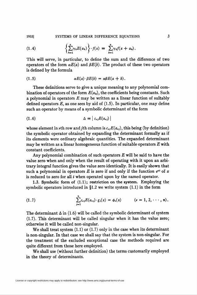
1933] SYSTEMS OF LINEAR DIFFERENCE EQUATIONS 3
(1.4) { T,ykE(ak) \ -f(x) m j^ykf(x + ak).\k-l J k-1
This will serve, in particular, to define the sum and the difference of two
operators of the form aE(a) and ßE(b). The product of these two operators
is defined by the formula
(1.5) aE(a) -ßE(b) = aßE(a + b).
These definitions serve to give a unique meaning to any polynomial com-
bination of operators of the form E(ak), the coefficients being constants. Such
a polynomial in operators E may be written as a linear function of suitably
defined operators E, as one sees by aid of (1.5). In particular, one may define
such an operator by means of a symbolic determinant of the form
(1.6) A - | ctjE(<h,) |
whose element in vth row and/th column is c¥JE(arj), this being (by definition)
the symbolic operator obtained by expanding the determinant formally as if
its elements were ordinary algebraic quantities. The expanded determinant
may be written as a linear homogeneous function of suitable operators E with
constant coefficients.
Any polynomial combination of such operators E will be said to have the
value zero when and only when the result of operating with it upon an arbi-
trary integral function gives the value zero identically. It is easily shown that
such a polynomial in operators E is zero if and only if the function ext of x
is reduced to zero for all t when operated upon by the named operator.
1.3. Symbolic form of (1.1); restriction on the system. Employing the
symbolic operators introduced in §1.2 we write system (1.1) in the form
n
(1 • 7) T,CnE(a,i) ■ gj(x) = 4>,(x) (v = 1, 2, • • • , »).i-i
The determinant A in (1.6) will be called the symbolic determinant of system
(1.7). This determinant will be called singular when it has the value zero;
otherwise it will be called non-singular.
We shall treat system (1.1) or (1.7) only in the case when its determinant
is non-singular. In that case we shall say that the system is non-singular. For
the treatment of the excluded exceptional case the methods required are
quite different from those here employed.
We shall use (without further definition) the terms customarily employed
in the theory of determinants.
License or copyright restrictions may apply to redistribution; see http://www.ams.org/journal-terms-of-use
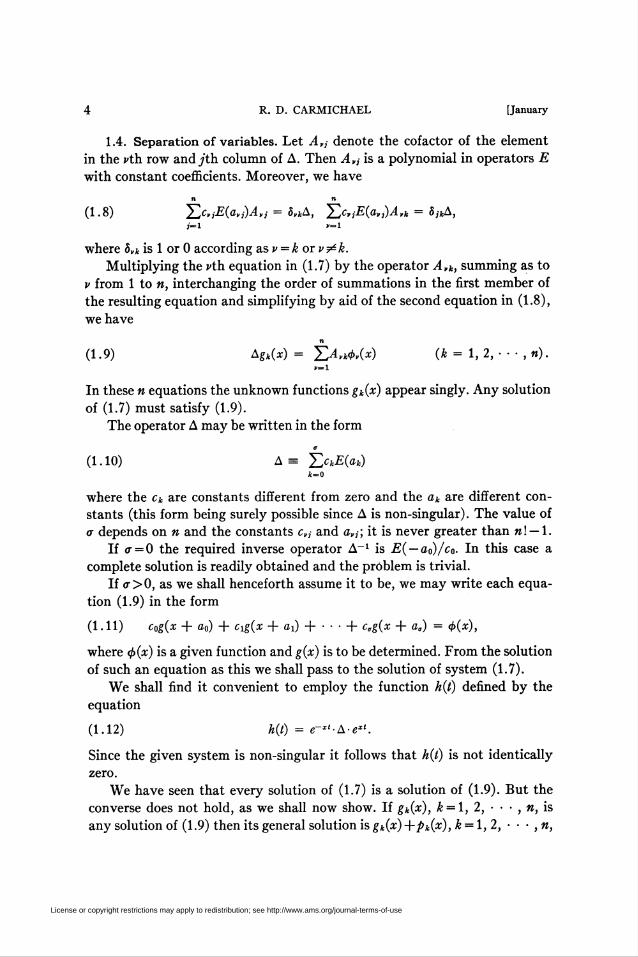
4 R. D. CARMICHAEL [January
1.4. Separation of variables. Let A,¡ denote the cofactor of the element
in the vth row and/th column of A. Then Avj is a polynomial in operators E
with constant coefficients. Moreover, we have
n n
(1.8) ^,c,jE(a„)A,j = 5,kA, ^cvjE(a„)Ark = SjkA,j-l V-1
where hrk is 1 or 0 according as v = k or v^k.
Multiplying the »-th equation in (1.7) by the operator Avk, summing as to
v from 1 to n, interchanging the order of summations in the first member of
the resulting equation and simplifying by aid of the second equation in (1.8),
we have
n
(1.9) Agk(x) = Y,Ark<t>Áx) (k = l,2,- ■■ ,n).i—i
In these n equations the unknown functions gk(x) appear singly. Any solution
of (1.7) must satisfy (1.9).
The operator A may be written in the form
(1.10) A= ¿c*£(a*)
where the ck are constants different from zero and the ak are different con-
stants (this form being surely possible since A is non-singular). The value of
a depends on n and the constants c„, and a,,-; it is never greater than n\ — 1.
If a = 0 the required inverse operator A-1 is E( — a0)/c0. In this case a
complete solution is readily obtained and the problem is trivial.
If o->0, as we shall henceforth assume it to be, we may write each equa-
tion (1.9) in the form
(1.11) c0g(x + a0) + Cig(x + ai) + ■ ■ ■ + ccg(x + a„) = <¿>(x),
where <f>(x) is a given function and g(x) is to be determined. From the solution
of such an equation as this we shall pass to the solution of system (1.7).
We shall find it convenient to employ the function h(t) defined by the
equation
(1.12) h(t) = e~x'-A-exi.
Since the given system is non-singular it follows that h(t) is not identically
zero.
We have seen that every solution of (1.7) is a solution of (1.9). But the
converse does not hold, as we shall now show. If gk(x), k = l, 2, ■ ■ ■ , n, is
any solution of (1.9) then its general solution is gk(x) +Pk(x), k = 1, 2, ■ ■ ■ , n,
License or copyright restrictions may apply to redistribution; see http://www.ams.org/journal-terms-of-use

1933] SYSTEMS OF LINEAR DIFFERENCE EQUATIONS 5
where the functions Pk(x) are arbitrary functions satisfying the equation
Apk(x) =0. Now consider the system
gi(x + 1) + g2(x) + g3(x +2) =4>i(x), gi(x + 2) + g2(x) + g3(x + 1) = <j>2(x),
g3(x) = 4>3(x).
Here we have A = E(1) —E(2) ¿¿0, whereas the function g3(x) is uniquely de-
termined by the last equation in the system.
From this example it follows that it is necessary to obtain an appropriate
solution of (1.9) in order to have a solution of (1.7). The problem falls
naturally into two cases; the following section prepares the way for this
separation of cases.
1.5. Functions of exponential type. If f(x) is an analytic function which
is regular at x0 and xu then it is easily shown that
lim sup | fM(xo) | 1/" = lim sup | /(v)(*i) I 1/",V= 00 P= OO
where the superscripts denote derivatives with respect to x. If these superior
limits have the finite value q (q^O) then f(x) is an integral function ; in such
a case we shall say that f(x) is of exponential type q, this terminology being
justified by the following theorem,* stated here without proof:
Theorem 1.1. A necessary and sufficient condition that the function f(x)
shall be of exponential type q is (1) that numbers r shall exist for which it is true
that for every positive number e there exists a quantity M, depending on e and r
in general but independent of x, such that for all (finite) values of x, we have
\f(x)\ < lfe<'+oui
and (2) that q shall be the least possible value for such numbers r. Moreover, when
f(x) is of exponential type q, we have
| /<">(*) \ < M(q + e)'e<»+«>l»l (v = 0, 1, 2, • • • ),
where M is independent of x and v.
1.6. Case when the <p» (x) are of exponential type. We first carry out the
solution of (1.7) for the case when the known functions </>„(x) are of ex-
ponential type not exceeding q. Taking their power series expansions in the
form
oo
(1.13) <pr(x) = 2>,*x7¿! (v = 1, 2, • • • , «),
* For a proof of this theorem and for further properties of functions of exponential type q, to-
gether with references to the literature, see a forthcoming paper of mine in Annals of Mathematics.
License or copyright restrictions may apply to redistribution; see http://www.ams.org/journal-terms-of-use

6 R. D. CARMICHAEL [January
we introduce the functions \¡/v(t) by means of the expansions
Ojt0 «Vl S»2
(1.14) *,(*) -_ + — + _+.... (r-1,2, •••,»).
Then the series in (1.14) all converge if |¿| >a. Let r be a positive number
exceeding q such that the circle Cr of radius r about 0 as a center passes
through no zero of the function h(t) defined in (1.12). (This negative condition
on r is first needed in the next paragraph.) Then we have
f>,(x) = —: f exL2irl Jcr
(1.15) *,(*) = — e*V,(t)dt (v - 1,2, • • • , n),2ttî Jcr
as one sees by using expansions (1.14) and integrating term by term in (1.15).
We employ the operator A„- with the meaning given in §1.4. By A^e1' we
mean the result of operating with A,f on ext considered as a function of x.
Now write
1 C A dt(1.16) gi(x) = — Z(^,c*0W)— (j = 1, 2, • • • , »),
¿ttî ^cr *=i «(/)
this being suggested by the problem of solving (1.9) by the method employed
by Pincherle (loc. cit.) for a similar equation. Now substitute in the first
member of (1.7) the functions g¡(x) so defined and simplify by aid of (1.8) and
(1.15); thus we have
« 1 /• « r «S^i-Efa«'/) •«>(*) -—; I X) y,c,)£(a,iMtreI( U.i_i 2xî Je, fc-i L ,=i J
= —; f ¿«,t(A«'0^2wiJcr *=i
dt
dt
= — Í exyv(t)dt = <pv(x).2ti Jcr
(x) defined by (1.16)
Equation (1.16) may be written in the form
£,(*) - — f «" ¿U^'l^o^W ■2ttî Je> fc-i «(0
Thence it follows that a constant M exists such that
|g,-w(0)| < Mr-r\
Therefore g,(x) is an integral function of exponential type not exceeding r.
Therefore the functions gs(x) defined by (1.16) afford a solution of (1.7).
dt
License or copyright restrictions may apply to redistribution; see http://www.ams.org/journal-terms-of-use
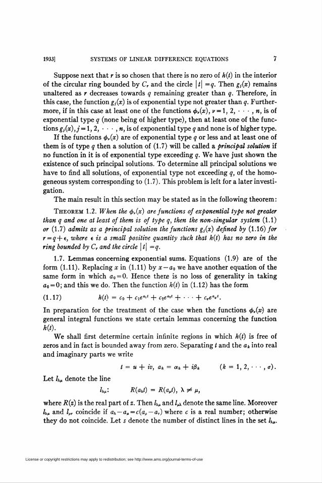
1933] SYSTEMS OF LINEAR DIFFERENCE EQUATIONS 7
Suppose next that r is so chosen that there is no zero of h(t) in the interior
of the circular ring bounded by Cr and the circle \t\ =q. Then g¡(x) remains
unaltered as r decreases towards q remaining greater than q. Therefore, in
this case, the function g¡(x) is of exponential type not greater than q. Further-
more, if in this case at least one of the functions <pv(x), v = 1, 2, •••,«, is of
exponential type q (none being of higher type), then at least one of the func-
tions gj(x),j = 1, 2, • • ■ , n, is of exponential type q and none is of higher type.
If the functions <¡>r(x) are of exponential type q or less and at least one of
them is of type q then a solution of (1.7) will be called a principal solution if
no function in it is of exponential type exceeding q. We have just shown the
existence of such principal solutions. To determine all principal solutions we
have to find all solutions, of exponential type not exceeding q, of the homo-
geneous system corresponding to (1.7). This problem is left for a later investi-
gation.
The main result in this section may be stated as in the following theorem :
Theorem 1.2. When the cpv(x) are functions of exponential type not greater
than q and one at least of them is of type q, then the non-singular system (1.1)
or (1.7) admits as a principal solution the functions g¡(x) defined by (1.16) for
r = q+e, where e is a small positive quantity such that h(t) has no zero in the
ring bounded by Cr and the circle \l\ =q.
1.7. Lemmas concerning exponential sums. Equations (1.9) are of the
form (1.11). Replacing x in (1.11) by x — a0 we have another equation of the
same form in which a0 = 0. Hence there is no loss of generality in taking
a0 = 0; and this we do. Then the function h(t) in (1.12) has the form
(1.17) h(t) = Co + cie"!' + c2e"1 + • • • + ce«-1.
In preparation for the treatment of the case when the functions (pv(x) are
general integral functions we state certain lemmas concerning the function
h(t).We shall first determine certain infinite regions in which h(t) is free of
zeros and in fact is bounded away from zero. Separating t and the ak into real
and imaginary parts we write
t = u+ iv, ak = ak+ ißk (k = 1, 2, • • • , a).
Let ¿xm denote the line
hß: R(axt) = RM, X ̂ p,
where R(z) is the real part of z. Then l\ß and l„\ denote the same line. Moreover
hß and lpT coincide if a\ — aß = c(ap — aT) where c is a real number; otherwise
they do not coincide. Let s denote the number of distinct lines in the set h?.
License or copyright restrictions may apply to redistribution; see http://www.ams.org/journal-terms-of-use

8 R. D. CARMICHAEL [January
Since each of these 5 lines passes through zero they divide the plane into 2s
sectors such that no point of any one of these lines is in the interior of any
such sector.
Let Si be any one of these 2s sectors and let h be any given interior point
of Si. Then no two of the quantities R(akti), k = 0, 1, • • • , a, are equal. Let
them be arranged in order of descending magnitude, thus :
R(akoti) > R(aklti) > > R(ak„h).
Then if h varies continuously over the interior of Si this continued inequality
will be preserved, since each member varies continuously and no two become
equal for an interior point of Si. One and just one term of this continued
inequality is zero for an interior point h of Si. Hence the first term is not
negative.
In the sector Si take a point P which is at a distance S from each of the
bounding rays of the sector, where h is a positive quantity whose value is to be
assigned later. From P draw rays to infinity in Si and parallel to the bounding
rays of Si, thus forming a new sector S interior to Si.
Let (u, v) be any point in S. Then the distance from (u, v) to the line
htk, is the positive quantity
(ako — ak,)u - (ßko - ßkl)v
{(ak0-ak,)2+(ßk0-ßk,y}1l2'
But this distance is not less than 5, whether /*„*, is or is not a bounding line
of Si. Therefore if t denotes the point (u, v) we have
R(ak„t) - R(aklt) = (ako - ak,)u - (ßko - ßk,)v
= ô{(aka - akí)2 + (ßk0 - ßkl)2}"2.
Now let t; be a fixed quantity such that
|cT|(l+<r") - (| Co| +|Cl| + •••+! c„|)e-'>0 (r = 0, 1, ■ ■ ■ , a).
Let m be the least value attained by the left member as r varies over the set
0, 1, • • • , a. Determine h so that
*{(«x - a,)2 + 03x - ft,)2}1'2 ^ v, X * p,
for every pair of different numbers X and p. from the set 0, 1, • • • , a. Then
R(ak,t)-R(akjt) ^ -r¡ for all t in S. Hence R(akt) -R(ak¿) ^ -77 for all / in 5
and for all k in the set 0, 1, • • • , a except k = ko.
From these inequalities and the fact that R(ak,t) = 0 in 5 it follows readily
that for all / in S we have
(1.18) I h(t)\ =m>0.
License or copyright restrictions may apply to redistribution; see http://www.ams.org/journal-terms-of-use
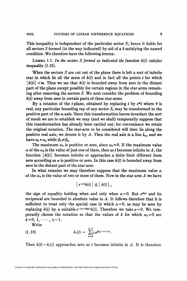
1933] SYSTEMS OF LINEAR DIFFERENCE EQUATIONS 9
This inequality is independent of the particular sector S; hence it holds for
all sectors 5 formed (in the way indicated) by aid of a 5 satisfying the named
condition. We therefore have the following lemma:
Lemma 1.1. In the sectors S formed as indicated the function h(t) satisfies
inequality (1.18).
When the sectors 5 are cut out of the plane there is left a sort of infinite
star in which lie all the zeros of h(t) and in fact all the points / for which
\h(t)\ <m. Thus we see that h(t) is bounded away from zero in the distant
part of the plane except possibly for certain regions in the star-arms remain-
ing after removing the sectors S. We next consider the problem of bounding
h(t) away from zero in certain parts of these star-arms.
By a rotation of the i-plane, obtained by replacing t by eat where 6 is
real, any particular bounding ray of any sector Si may be transformed to the
positive part of the «-axis. Since this transformation leaves invariant the sort
of result we are to establish we may (and we shall) temporarily suppose that
this transformation has already been carried out; for convenience we retain
the original notation. The star-arm to be considered will then lie along the
positive real axis; we denote it by A. Then the real axis is a line /x„, and we
have ax=a„ while p\ 9e pV
The maximum a* is positive or zero, since a0=0. If the maximum value
a of the ak is the value of just one of them, then as t becomes infinite in A, the
function \h(t)\ becomes infinite or approaches a finite limit different from
zero according as a is positive or zero. In this case h(t) is bounded away from
zero in the distant part of the star-arm.
In what remains we may therefore suppose that the maximum value a
of the ak is the value of two or more of them. Now in the star-arm A we have
| e-°>h(t) | ^ | h(t) | ,
the sign of equality holding when and only when a = 0. But e*3*' and its
reciprocal are bounded in absolute value in A. It follows therefore that it is
sufficient to treat only the special case in which a = 0, as may be seen by
replacing h(t) by a suitable e~{a+ißk)th(t). Therefore we take a = 0. We tem-
porarily choose the notation so that the values of k for which ak = 0 are
A-0, l,.-.,7-l.Write
7-1
(1.19) hi(t) = X)^*<_"+iu) •
Then h(t)—hi(t) approaches zero as t becomes infinite in A. It is therefore
License or copyright restrictions may apply to redistribution; see http://www.ams.org/journal-terms-of-use

10 R. D. CARMICHAEL [January
sufficient to our purpose to determine suitable parts of A in which h(t) is
different from zero and hi(t) is bounded away from zero.
For this investigation we need the following classical lemma which
we state without proof :
Lemma 1.2. If bi,b2, •■■ ,br is any set of real numbers, all different from
zero, and if h is any preassigned positive number, then there is an infinitude of
positive integers m such that, for each such m, integers ki, k2, • ■ • , k, exist such
that
(1.20) |M/ + «|^8 (j=l,2,---,v).
If all such positive integers m are denoted by the symbols mi, m2, ■ ■ ■ , with
mi<m1+i,j = l, 2, • ■ • , then among the differences mj+i —m,- there is a greatest
one.
Applying this lemma to the case when ¿, = l//3, and p=y — l, we have
Iki + mßil^ißi 0'= 1,2, •••,7-1).
Thence it follows that for every preassigned positive e there exists a h such
that we now hâve
7-1
I hi(t + 2mir) - hi(t) | ^ X) I ckeiB"'(e2äi'm'i - 1) | < ék—0
for all t in the star-arm A. Let R be a rectangle two sides of which are on the
boundaries of A and let it be subject to the condition that hx(t) does not
vanish in R. Let e be such that | hi(t) | >2e in R. Then
| hi(t + 2mw) | > «
when t is in R and m is an integer admitted by the foregoing lemma.
We now return to the original form of h(t) as given in (1.17). On each arm
of the star associated with h(t) we now take a rectangle R obtained from the
foregoing one by reversing the rotation by which the corresponding arm is
put in the special position employed in the preceding argument; or, we take
any rectangle R on the arm and in which h(t) does not vanish, in case the
situation is-such that the preceding argument reaches the goal before the
introduction of Lemma 1.2 and the rectangle R. Then h(t) is bounded away
from 0 on R and on all congruent rectangles (except a finite number at most)
similar to those in the preceding paragraph and containing the points t+2mir
with t on R and m determined as in the lemma or m sufficiently large when
the lemma is not needed.
License or copyright restrictions may apply to redistribution; see http://www.ams.org/journal-terms-of-use
1933] SYSTEMS OF LINEAR DIFFERENCE EQUATIONS 11
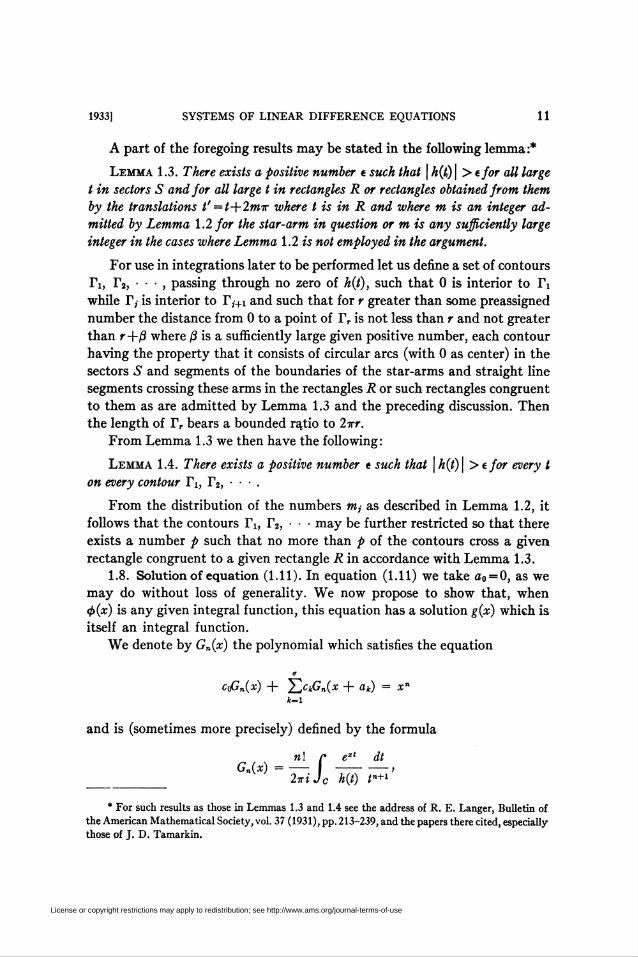
A part of the foregoing results may be stated in the following lemma :*
Lemma 1.3. There exists a positive number e such that \ h(t) \ > efor all large
t in sectors S and for all large t in rectangles R or rectangles obtained from them
by the translations t'=t+2mx where t is in R and where m is an integer ad-
mitted by Lemma 1.2 for the star-arm in question or m is any sufficiently large
integer in the cases where Lemma 1.2 is not employed in the argument.
For use in integrations later to be performed let us define a set of contours
Ti, r2, ■ • ■ , passing through no zero of h(t), such that 0 is interior to Ti
while T, is interior to r,+i and such that for r greater than some preassigned
number the distance from 0 to a point of TT is not less than r and not greater
than r+ß where ß is a sufficiently large given positive number, each contour
having the property that it consists of circular arcs (with 0 as center) in the
sectors 5 and segments of the boundaries of the star-arms and straight line
segments crossing these arms in the rectangles R or such rectangles congruent
to them as are admitted by Lemma 1.3 and the preceding discussion. Then
the length of Yr bears a bounded ra.tio to 27rr.
From Lemma 1.3 we then have the following:
Lemma 1.4. There exists a positive number e such that ] h(t) | >tfor every t
on every contour Ti, T2, • • ■ .
From the distribution of the numbers m¡ as described in Lemma 1.2, it
follows that the contours Ti, r2, • ■ • may be further restricted so that there
exists a number p such that no more than p of the contours cross a given
rectangle congruent to a given rectangle R in accordance with Lemma 1.3.
1.8. Solution of equation (1.11). In equation (1.11) we take a0 = 0, as we
may do without loss of generality. We now propose to show that, when
4>(x) is any given integral function, this equation has a solution g(x) which is
itself an integral function.
We denote by Gn(x) the polynomial which satisfies the equation
a
coGn(x) + J^ckGn(x + ak) = x"k-l
and is (sometimes more precisely) defined by the formula
»! r exl dtGn(x) =- I-j
_ 2wiJc h(t) t»+l
* For such results as those in Lemmas 1.3 and 1.4 see the address of R. E. Langer, Bulletin of
the American Mathematical Society, vol. 37 (1931), pp. 213-239, and the papers there cited, especially
those of J. D. Tamarkin.
License or copyright restrictions may apply to redistribution; see http://www.ams.org/journal-terms-of-use

12 R. D. CARMICHAEL [January
where « is a positive integer or zero, h(t) denotes the function defined in (1.17)
and C is a contour inclosing the point 0 and no singularity of the integrand
other than / = 0.
Let Tr, where r is any positive integer, denote the contour represented by
this symbol in the latter part of §1.7. Form the function
n\ r ext dtGn.r(x) =-
2xiJr, h(t) t"+l
This function satisfies the equation
a
CcPn.r(x) + ^fin,r(x + Ok) = Xn.k=l
Let x be now confined to any preassigned finite region T of the x-plane.
Then we have
i »! CGn.r(x)\ Ú—Mt
2x Jr.
dt\
t\n+l
where Mi is a dominant of | l/h(t) | for all / on all contours TV, the existence
of this dominant being assured by Lemma 1.4. From the character of the
contours Tr, as described in the latter part of §1.7, we now see that a con-
stant M (independent of x and n and r) exists such that for all x in T we have
(1.21) | <?„.,(*) | < M-n\-p'+ar-",
where p is such that p >e|z| for all x in T.
Write the power series expansion of <p(x) in the form
«0
(1.22) *(*) = 2>,*\1—0
Form the function g(x),
00
(1.23) g(x) = 2XG,,,(x).»-0
Then the (»»+l)th term of the series here written is, in the region T and for
sufficiently large values of v, less in absolute value than the quantity
M-v\v-'p'+ß\ Xk| .
As v becomes infinite the superior limit of the pth root of this quantity is zero
since |X„|ll" has the superior limit zero owing to the fact that <p(x) is an in-
tegral function. Therefore the series in (1.23) converges absolutely and uni-
License or copyright restrictions may apply to redistribution; see http://www.ams.org/journal-terms-of-use
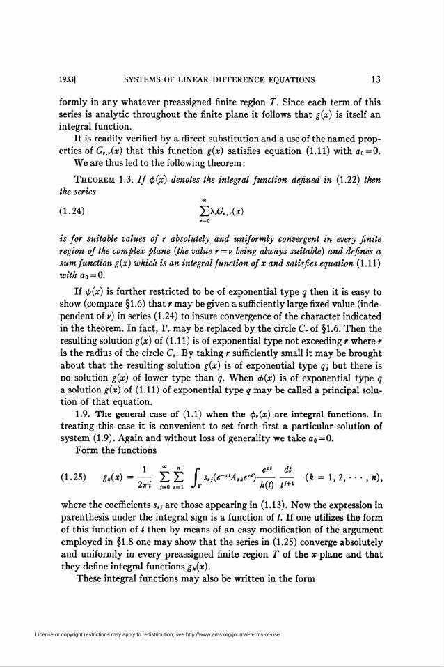
1933] SYSTEMS OF LINEAR DIFFERENCE EQUATIONS 13
formly in any whatever preassigned finite region T. Since each term of this
series is analytic throughout the finite plane it follows that g(x) is itself an
integral function.
It is readily verified by a direct substitution and a use of the named prop-
erties of G,,,(x) that this function g(x) satisfies equation (1.11) with a0 = 0.
We are thus led to the following theorem :
Theorem 1.3. If <p(x) denotes the integral function defined in (1.22) then
the seriesCO
(1.24) !>£„,(*)r-0
is for suitable values of r absolutely and uniformly convergent in every finite
region of the complex plane (the value r=v being always suitable) and defines a
sum function g(x) which is an integral function of x and satisfies equation (1.11)
with a0 = 0.
If <p(x) is further restricted to be of exponential type q then it is easy to
show (compare §1.6) that r may be given a sufficiently large fixed value (inde-
pendent of v) in series (1.24) to insure convergence of the character indicated
in the theorem. In fact, TT may be replaced by the circle Cr of §1.6. Then the
resulting solution g(x) of (1.11) is of exponential type not exceeding r where r
is the radius of the circle Cr. By taking r sufficiently small it may be brought
about that the resulting solution g(x) is of exponential type q; but there is
no solution g(x) of lower type than q. When <p(x) is of exponential type q
a solution g(x) of (1.11) of exponential type q may be called a principal solu-
tion of that equation.
1.9. The general case of (1.1) when the <¡>P(x) are integral functions. In
treating this case it is convenient to set forth first a particular solution of
system (1.9). Again and without loss of generality we take a0=0.
Form the functions
1 °° " c ext dt(1.25) gk(x) =- IE s.iie-tA,*«)— — ■(* = 1, 2, • • • , «),
2irt ;_o ,_x Jr h(t) P+l
where the coefficients s„,- are those appearing in (1.13). Now the expression in
parenthesis under the integral sign is a function of /. If one utilizes the form
of this function of t then by means of an easy modification of the argument
employed in §1.8 one may show that the series in (1.25) converge absolutely
and uniformly in every preassigned finite region T of the «-plane and that
they define integral functions gk(x).
These integral functions may also be written in the form
License or copyright restrictions may apply to redistribution; see http://www.ams.org/journal-terms-of-use
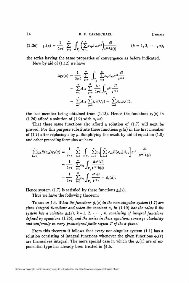
14 R. D. CARMICHAEL [January
(1.26) gk(x)=—■ ¿ f (Í2sy¡AykeA-2iri ,_o Jr. \_i /t'
dt- (k = 1, 2, • • • , «),
+ih(t)
dt
iH-l
the series having the same properties of convergence as before indicated.
Now by aid of (1.12) we have
1 " r " dt^gk(x) = —; X, I ¿^S'iA'lfi" —
2-ai ,_o Jr. ^i t'+l
= ¿^¿-^ fe"-r-l ,_o 2xi Jr. /'
n w n
»—1 j=0 >=1
the last member being obtained from (1.13). Hence the functions gk(x) in
(1.26) afford a solution of (1.9) with a0 = 0.
That these same functions also afford a solution of (1.7) will next be
proved. For this purpose substitute these functions gk(x) in the first member
of (1.7) after replacing v by p. Simplifying the result by aid of equation (1.8)
and other preceding formulas we have
n ico/*nrn ~\ dt
YsCkE^ùg^x) = —; X) I ZXi H cßkE(aßk)A,k \extk-i 2wt ,_0 Jr. _i L*_i J ¿)+1A(¿)
1 " r Aextdt
"iTi hoS" JT.lî+^Mt)1 " r extdt
= T— 2-ímí —77 = *!■(*) •2ttí ,_o Jr; P+l
Hence system (1.7) is satisfied by these functions gk(x).
Thus we have the following theorem :
Theorem 1.4. When the functions cpr(x) in the non-singular system (1.7) are
given integral functions and when the constant a0 in (1.10) has the value 0 the
system has a solution gk(x), k = l, 2, • ■ ■ , », consisting of integral functions
defined by equations (1.26), and the series in these equations converge absolutely
and uniformly in every preassigned finite region T of the x-plane.
From this theorem it follows that every non-singular system (1.1) has a
solution consisting of integral functions whenever the given functions <p,(x)
are themselves integral. The more special case in which the <pr(x) are of ex-
ponential type has already been treated in §1.6.
License or copyright restrictions may apply to redistribution; see http://www.ams.org/journal-terms-of-use

1933] SYSTEMS OF LINEAR DIFFERENCE EQUATIONS 15
II. Simultaneous expansions of integral functions in
COMPOSITE POWER SERIES
2.1. Formulation of the problem. For »>1 we consider the question of
expanding n integral functionsfi(x),f2(x), • • • ,fn(x) simultaneously in com-
posite power series, that is, we consider the problem of representing these
functions in the form
(2.1) /,(*)= ¿ ¿^»(äc - a,,)» (v = 1,2, •••,«),*-0 j-l
where the coefficients cjk are to be independent of both x and v. We impose the
further condition on the coefficients cjk that they shall be such that the series
in the equations00
(2.2) gi(x) = Xc,*x* (j= 1,2, ••-,«)*=0
shall converge for all finite values of x; then the sum functions g,(x) defined
by them will be integral functions. These conditions on the c]k are equivalent
to the conditions that the quantities \cjk\llk, j = l, 2, • • • , «-, shall all have
the limit zero as k becomes infinite. Furthermore we subject the given con-
stants avj to the condition that the determinant A(t) whose element in vth
row and/th column is exp(—arjt) shall not be identically zero as a function of
t. In the exceptional or singular case in which this condition on A(t) is not
satisfied the general investigation will require methods different from those
here employed; and the results will lack the simplicity and elegance which
belong to the general case here treated.
For n = 1 the problem evidently reduces to the classical problem of ex-
pansions in power series. We suppose throughout that n>l.
Under the conditions named we shall show that such simultaneous ex-
pansions always exist and indeed that they always exist subject to the further
condition that the functions g¡(x), j = l, 2, ■ ■ ■ , n, shall be of exponential
type provided in the latter case that the functions f,(x), v = l, 2, • • -, n, are
of exponential type.
If we employ the notation defined in (2.2) we may write (2.1) in the form
n
(2.3) fr(x) = £g,(x - a,,) (r- 1,2, •••,»).j-i
Integral solutions of this system evidently lead through (2.2) to the required
expansions (2.1). The condition put on A(¿) is just that which is required to
make the results of the first part of this paper applicable to system (2.3) and
hence to the expansion problem here set.
License or copyright restrictions may apply to redistribution; see http://www.ams.org/journal-terms-of-use

16 R. D. CARMICHAEL [January
2.2. Expansions in the case of general integral functions/,^). From The-
orem 1.4 and the remark following it one concludes that system (2.3) has in
this case integral solutions gj(x), j = l, 2, • • • , n. Therefore we have the
following theorem:
Theorem 2.1. Iffi(x),f2(x), • • ■ ,fn(x) are any given integral functions and
if the constants a„- are such that the determinant A(t) has the property described
in the first paragraph of §2.1, then these functions f,(x) have simultaneous ex-
pansions of the form (2.1) where
lim |c,»|»* = 0 (j' = 1,2, •••,»).
Formulas in §1.9 afford an effective means of obtaining suitable coeffi-
cients Cjk to be employed in the expansions (2.1). Only in exceptional cases is
it true that these expansions are unique. The determination of the extent of
arbitrary elements involved in the coefficients of the expansions depends on
the (as yet undeveloped) theory of system (2.3) for the case when f,(x) =0,
" = 1,2, •••,».
2.3. Expansions when thef,(x) are of exponential type. Applying The-
orem 1.2 to system (2.3) in the case when the functions f,(x) are of exponential
type and interpreting the results in terms of the expansions in (2.1), we have
the following theorem:
Theorem 2.2. If the functions fi(x), ft(x), ■ ■ ■ , fn(x) are of exponential
type not exceeding q, one at least of them being precisely of type q, and if the
constants a,,- are such that the determinant A(t) has the property described in the
first paragraph of §2.1, then the functions f,(x) have simultaneous expansions of
the form (2.1) such that the associated functions g¡(x) of (2.2) are of exponential
type and indeed such that these functions g,(x) are of exponential type not ex-
ceeding q, one at least of them being precisely of type q.
When the associated gs(x) are of exponential type not exceeding q we
shall say that the series in (2.1) afford principal expansions of the functions
Even with the strongest conditions imposed on the coefficients cjk by the
latter part of the foregoing theorem it is still true that the expansions (2.1)
need not be unique. In all cases belonging to this section possible values of the
coefficients c,* are readily determined from the special case of equation
(1.16) applicable here, as we show in the next paragraph; and these values
may well vary in dependence upon the radius r of the circle Cr appearing in
(1.16).
License or copyright restrictions may apply to redistribution; see http://www.ams.org/journal-terms-of-use

1933] SYSTEMS OF LINEAR DIFFERENCE EQUATIONS 17
In connection with the expansions
00
/»(*) = E«,»**/*! (* = 1, 2, • • • , «),*-o
form the functions00
F,(t)= E—: (" = 1,2, ••-,«).*-o ™
Let A„,(/) be the cofactor of the element in the vth row and jth column of
A(t). Then by aid of (1.16) it may readily be shown that suitable coefficients
Cjk in (2.1) are the following:
i r ( A \ tkdt
'"-^mL(^ÁmVWwhere/ = 1, 2, • • • , n and k = 0, 1, 2, • • • .
2.4. The case avj = a„ for v>j. In this case system (2.3) is equivalent to
the system consisting of the first equation in (2.3) and the following « — 1
equations:
n
(2.4) /,_,(x) - /,(*) = £{g,(x - <*_!,,) - gi(x - a,,)) (y = 2, 3, • • • , n).
In case a„_i,„ = a„n it is clear that we must have/„_i(x) =fn(x) as a necessary
condition for satisfying the system. In fact, it is easy to see that the functions
fy(x) must satisfy one or more special restrictive conditions if one or more of
the relations
(2.5) «M.r-i^O (r- 2,3, •••,»)
fails to be satisfied. But if conditions (2.5) are all satisfied then we have an
instance of the general theory already developed; we shall suppose that these
conditions are satisfied. We assume that the given functions fi(x), ■••,/»(*)
are all integral functions. We require that the functions gi(x), ■ ■ • , gn(x)
shall be integral functions.
Taking v = n in (2.4) we see that gn(x) is uniquely determined as an in-
tegral function except for an arbitrary additive periodic integral function of
period a„_i,„ — a„„. Taking gn(x) to be any integral function satisfying (2.4)
for p = n we may then determine gn-i(x) uniquely except for an additive in-
tegral function of period a„_2,n-i — a»_i,«_i. With gn-i(x) determined we pro-
ceed similarly to the determination of gn~2(x), and we continue thus until
g2(x) is determined. Then the first equation in (2.3) uniquely determines
gi(x). It appears, therefore, that in the present case one can determine com-
License or copyright restrictions may apply to redistribution; see http://www.ams.org/journal-terms-of-use

18 R. D. CARMICHAEL [January
pletely the arbitrary elements in the solution of (2.3) subject to the named
conditions. Hence all possible expansions (2.1) are completely determined for
the present case.
If we further restrict the given functions fi(x), ■ ■ ■ , fn(x) to be of ex-
ponential type not greater than q we may likewise determine the functions
gi(x), ■ ■ : , gn(x) so that they are of exponential type not greater than q and
we may show precisely what is arbitrary in the determination of such func-
tions subject to these conditions. These results may then be carried over to
the corresponding case of the expansions (2.1).
There is one case of particular interest in which the expansions (2.1),
when subject to the condition named in the preceding paragraph, are unique
except for the trivial restriction that the constants cl0,j = l, 2, ■ • • , », are
not separately determined but only their sum is determined. This is the case
in which the functions fi(x), ■ ■ ■ , fn(x) are of exponential type not greater
than q while at the same time the relations
(2.6) q\ a,-i,, — a„\ < 2ir (v = 2, 3, • • • , «)
are all satisfied. For in this case each g,(x) is uniquely determined except for
an additive constant. These conditions are obviously satisfied whenever
inequalities (2.5) hold provided that q = 0 and in particular provided that
the functions/,(x) are polynomials.
2.5. The case » = 2. For the case n = 2 system (2.3) may be written in the
form7 fi(x + an) = gi(x) + gi(x + an - an),
f2(x + a2i) = gi(x) + g2(x + a2i — a22).
The exceptional case here is that in "which an — ai2 = a2i — a22. When this
condition is satisfied, the system can have a solution only when fi(x+au)
=fi(x+Oii), as one sees from (2.7); and in this case it is clear that either of
the integral functions gi(x) and g2(x) may be assigned at will and that the
other is then uniquely determined: the case is therefore trivial.
When aii — an^a-ti — avt the case belongs to that treated in §2.4.
As an application of the case when an = a, an = b,an = 0 = a22, where a^b,
we see that an arbitrary integral function f(x) may be expanded in the form
oo
(2.8) f(x) = T,{ck(x - a)" + yk(x - b)")fc=0
where the sums ck+yk, k = 0, 1, 2, • • -, have any preassigned values subject
to the condition that
lim lofe + T*!1'*
License or copyright restrictions may apply to redistribution; see http://www.ams.org/journal-terms-of-use
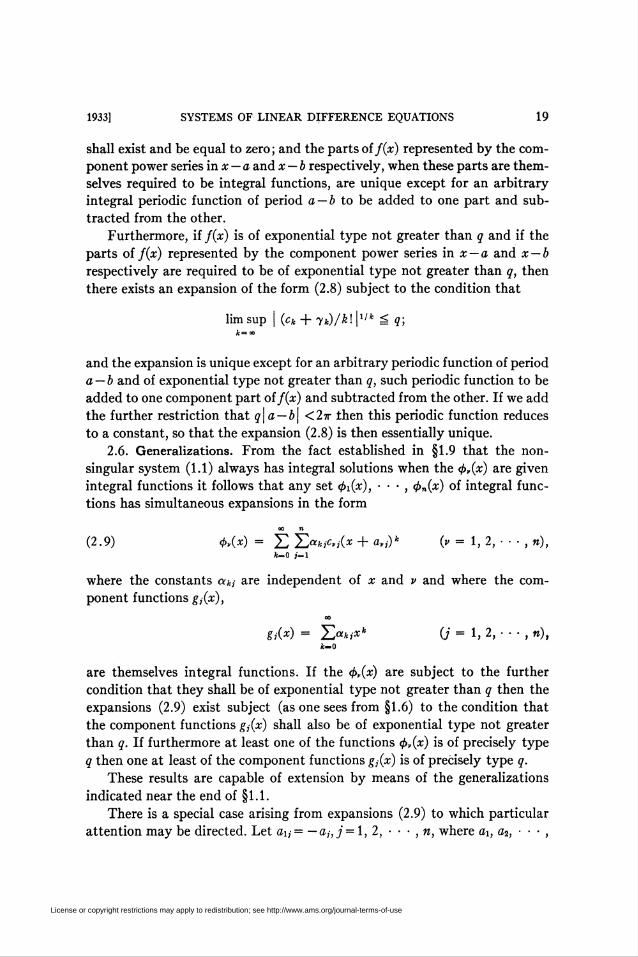
1933] SYSTEMS OF LINEAR DIFFERENCE EQUATIONS 19
shall exist and be equal to zero; and the parts of f(x) represented by the com-
ponent power series in x — a and x — b respectively, when these parts are them-
selves required to be integral functions, are unique except for an arbitrary
integral periodic function of period a — b to be added to one part and sub-
tracted from the other.
Furthermore, if f(x) is of exponential type not greater than q and if the
parts of f(x) represented by the component power series in x — a and x — b
respectively are required to be of exponential type not greater than q, then
there exists an expansion of the form (2.8) subject to the condition that
lim sup | (ck + yk)/k\\ltk = q;k-t
and the expansion is unique except for an arbitrary periodic function of period
a — b and of exponential type not greater than q, such periodic function to be
added to one component part off(x) and subtracted from the other. If we add
the further restriction that q\a — b\ <2ir then this periodic function reduces
to a constant, so that the expansion (2.8) is then essentially unique.
2.6. Generalizations. From the fact established in §1.9 that the non-
singular system (1.1) always has integral solutions when the <f>r(x) are given
integral functions it follows that any set 0i(x), • • -, <f>n(x) of integral func-
tions has simultaneous expansions in the form
oo n
(2.9) 4>y(x) = E Hj*kiC,j(x + a„)k (v = 1,2, ■ ■ ■ , n),k=0 i=l
where the constants aki are independent of x and v and where the com-
ponent functions g¡(x),
00
ii(x) = 2>*,x* (j = 1, 2, • • • , n),k-0
are themselves integral functions. If the <f>,(x) are subject to the further
condition that they shall be of exponential type not greater than q then the
expansions (2.9) exist subject (as one sees from §1.6) to the condition that
the component functions g,(x) shall also be of exponential type not greater
than q. If furthermore at least one of the functions <p,(x) is of precisely type
q then one at least of the component functions g,(x) is of precisely type q.
These results are capable of extension by means of the generalizations
indicated near the end of §1.1.
There is a special case arising from expansions (2.9) to which particular
attention may be directed. Let ai, = —a,-,/ = l, 2, • • • , n, where ai, a2, ■ ■ ■ ,
License or copyright restrictions may apply to redistribution; see http://www.ams.org/journal-terms-of-use
20 R. D. CARMICHAEL [January
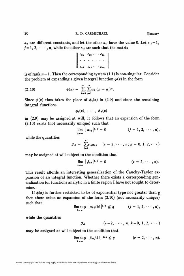
an are different constants, and let the other arj have the value 0. Let Ci, = 1,
j = l, 2, • • • , n, while the other crj are such that the matrix
|| C2i c22 ■ ■ • c2n I
II Cnl Cn2 • ■ ■ Cnn II
is of rank « — 1. Then the corresponding system (1.1) is non-singular. Consider
the problem of expanding a given integral function <p(x) in the form
(2.10) <f>(x) = Hak Ax - a,-)*.*=0 1-1
Since <j>(x) thus takes the place of <pi(x) in (2.9) and since the remaining
integral functions
<h(x), ■ ■ • , <f>n(x)
in (2.9) may be assigned at will, it follows that an expansion of the form
(2.10) exists (not necessarily unique) such that
lim |«m|w*-0 (j = 1, 2, ••• ,»),jt=oo
while the quantitiesn
ßvk = ^er,akj (v = 2, ■ ■ ■ , n; k = 0, 1, 2, ■ • • )i-i
may be assigned at will subject to the condition that
lim | ßrk \llk = 0 (v = 2, • • • ,«).
This result affords an interesting generalization of the Cauchy-Taylor ex-
pansion of an integral function. Whether there exists a corresponding gen-
eralization for functions analytic in a finite region I have not sought to deter-
mine.
If <j>(x) is further restricted to be of exponential type not greater than q
then there exists an expansion of the form (2.10) (not necessarily unique)
such thatlim sup | ahi/k\ \llk ^ q (j = 1, 2, ■ • • , »),
while the quantities
ß,k (v = 2, ■ • .,»;Ä=0, 1, 2, • • •)
may be assigned at will subject to the condition that
lim sup | ß,k/k\ | llk ^ q (v = 2, • • • , »).
License or copyright restrictions may apply to redistribution; see http://www.ams.org/journal-terms-of-use

1933] SYSTEMS OF LINEAR DIFFERENCE EQUATIONS 21
III. Expansions in series of exponential functions
3.1. Properties of exponential sums. Let us denote by h(t) the function
(3.1) h(t) = CiC"' + c2e^ + ■ ■ • + ce0»', n > 1,
where au a*, ■ • • , a„ are different constants and Ci, c2, ■ ■ ■ , c„ are constants
different from zero. And let us consider the problem of bounding away from
zero the function e~xth(t) for suitable given values of x and for suitable ranges
of /. The results are needed for our later investigation (§3.2) of certain contour
integrals.
Let P be the smallest convex polygon, in the complex plane, containing
the points au a2, • ■ ■ , a„; this polygon may in special cases reduce to a
straight line segment. Let Q be the polygon* obtained by reflecting P through
the real axis. For the sake of definiteness we suppose that the notation is so
chosen that the vertices of P, taken in counter-clockwise order, are ax, a2,
■ • • , ay (v^n) and that no a, has its real part less than that of ai. Moreover
we suppose that the vertices are so taken that no three of these a's at the
vertices lie on the same straight line..Let h, h, ■ ■ • ,h be the rays normal to
the sides of Q at their centers and drawn outward from this polygon; when Q
reduces to a straight line it is to be understood that these rays are two in
number and that they are drawn so that there is one in each direction from
the middle point of the line. We take the notation so that h, l2, ■ ■ ■ ,h are in
clockwise order and so that h is the normal to the side joining the conjugates
of ai and a2.
Let a,- and ak be two consecutive vertices of P and let lß be the normal to
that side of Q which joins the corresponding vertices of Q. If R(z) denotes the
real part of z, then the line R(ajt) =R(akt) is parallel to the line /„. Let p be a
positive number whose value is later to be conveniently restricted. On each
side of each line h, l2, • ■ • , I, and at a distance p from it draw a ray in such a
way that these rays will make a sort of infinite star similar to that considered
in §1.7 and containing the rays h, l2, ■ ■ ■ , I, in the centers of its arms. These
rays form certain sectors S, similar to those in §1.7 and containing no in-
terior points of the named infinite star.
In order to have sectors exactly like those in §1.7 it is necessary to divide
some of the sectors S into smaller sectors by excluding other strips; but this
further division is to serve only a temporary purpose in the argument. It may
be described as follows. Let mi, m2, • • ■ , m, be rays from zero to infinity
parallel to h, l2, ■ ■ • , I, respectively but such that mk goes to infinity in a
direction opposite to that of lk- Some rays mk may go to infinity in the same
* Such polygons as P and Q have been employed by Pólya, Mathematische Annalen, vol. 89
(1923), pp. 179-191.
License or copyright restrictions may apply to redistribution; see http://www.ams.org/journal-terms-of-use

22 R. D. CARMICHAEL [January
direction as other rays l¡ (and they will do so when Q has pairs of parallel
sides); remove such rays mk', if any rays ma remain after this removal, denote
them hy ma, mß, • ■ ■ . Along the rays ma, mß, ■ ■ ■ remove strips of width 2p
as in the case of the preceding paragraph. Then some sectors 5 are separated
into two or more sectors (together with one or more strips). After all such
separations are made-, let S' he a symbol to denote the totality of sectors ob-
tained, including undivided sectors S and the parts into which some sectors
5 have been separated.
From Lemma 1.1 it follows that p may be taken sufficiently large that
h(t), and hence e~~xth(t), shall have no zero in any sector S'. Moreover, from
the same lemma it follows that p may be taken sufficiently large (and we so
take it) that e~xth(t) is bounded away from zero in the sectors S' when x is any
one of the points ai, a2, • • • , an. In fact, when x has any such value the func-
tion e^'hQ) is a function meeting the conditions on h(t) in §1.7 so that
Lemmas 1.3 and 1.4 are also applicable to e~xth(t) for such values of x.
Let öj-, ak and a¡ be any three consecutive vertices of P in counter-
clockwise order and let /,- and lk be the rays perpendicular to the sides of Q
with corresponding vertices. Let Slk he the sector 5 lying between /,- and /*.
Suppose that t varies in Sjk. Let x be a fixed point in P. We have
| e~xth(t) | = | »<•*-«><»-•*) | . | e»i<«r*' | • | e-"k'h(t) \ ,
where dk is the conjugate of ak. The last factor in the second member is
bounded away from zero for large / in the named sector, as we have already
seen. The middle factor is a constant different from zero, since x is fixed. The
argument of the exponent of the first factor lies between — \tr and §tt in-
clusive, as one may readily show graphically, if (as we do by taking p suffi-
ciently large) we restrict the sector Sjk to lie in the sector formed by rays
from dk to infinity in the direction of the rays /,- and lk: in establishing the
named fact it is convenient temporarily to transform the points of the plane
by adding — a* to each value in it so that the representation of dk becomes the
point zero and then to begin from the plots of x — âk and t — âk. Thence it
follows that e~xth(t) is bounded away from zero in the named sector. Further-
more it follows from Lemma 1.3 that e~x'h(t) is bounded away from zero for
all large / in rectangles congruent to the rectangles R in the way specified in
that lemma, these rectangles R being chosen with reference to the function
erxth(t).
Let us now further restrict x to lie in the interior of P. Then there exists
a positive number é such that
— Í7T + e á arg {(ak — x)(t — ak) } á i*- — «•
License or copyright restrictions may apply to redistribution; see http://www.ams.org/journal-terms-of-use

1933] SYSTEMS OF LINEAR DIFFERENCE EQUATIONS 23
Thence it follows that the function t~le~xih(i) is bounded away from zero as /
becomes infinite in the named sector.
The same function is also bounded away from zero if x is on the boundary
of P but not at ak while / becomes infinite in the named sector in such a way
as to remain outside of each of two parabolas with vertex at äk and having the
named rays from äk parallel to lj and lk as their principal diameters.
It may now be observed that every strip along one of the rays ma,mß, ■ ■ ■
lies (except for a finite part of it) entirely in a sector S and that it has a direc-
tion intermediate to the directions of the bounding rays of this sector S.
Thence it follows also that such a strip (except for a finite part of it) lies
entirely outside of the parabolas along the bounding rays of this sector 5.
Hence the strips along the rays ma, m8, • • • may be removed and we thus
return to the set of sectors 5 as defined in this section ; and for the plane so
divided we have the requisite character of c-1'^) or trle~~**h(t) as a function
bounded away from zero, in accordance with the paragraph next following.
Summing up these results we may state that e~xth(t) is bounded away
from zero for any given x in P and for all large t in all sectors S formed with
sufficiently large p and in all rectangles congruent to rectangles R in accor-
dance with Lemma 1.3; that t~xe~xih(() is bounded away from zero for each
interior point x of P and for all large / in all such sectors S; and that t~xe~xth(i)
is bounded away from zero for each x on the boundary of P and not at a ver-
tex of P and for all large t in all such sectors S and outside of all parabolas of
the sort described for äk in the previous paragraph, two such parabolas being
formed at each vertex of Q.
3.2. Properties of certain contour integrals. Let Ci, C2, • • • , C„, ■ • • be
a set of different contours in the complex plane such that any given point on
Cj is either interior to Cy+i or on C,+1 and such that for every s there exists an
r such that the contour C, is a contour Tr of the sort described in §1.7 and
suitable to apply to e~xth(t) for points x in P as the contours I\ apply to the
function h(t) of §1.7 and such that for every r there is an s such that C, is a
contour Tr.
Let \j/(t) be any function of t which is analytic at infinity and vanishes
there and let us write
(3.2) W) = yi/t + y2/t2 + y,/fi + ■ ■ • , 11\ > q.
Let r be a fixed integer such that the contour CT lies entirely within the region
of convergence of the series in (3.2). Form the function Zr(x),
(3.3) Fr(x) = — f ex'{h(t)}-lp(t)dt.2tí Jct
Then Zr(x) is a function of exponential type; and, in fact, it is such a function
License or copyright restrictions may apply to redistribution; see http://www.ams.org/journal-terms-of-use

24 R. D. CARMICHAEL [January
as arises from the solution of equation (1.11) when <j>(x) is a given function of
exponential type, as one sees from Part I and especially from §1.6.
Let p be any positive integer and form the function Fr+P(x) by changing
r to r+p in (3.3). We shall show that
(3.4) lim Fr+P(x) = 0p— oo
when any one of the following conditions is satisfied :
(1) when x is in the interior of P;
(2) when x is on the boundary of P and is not a vertex of P ;
(3) when a; is a vertex of P provided in this case that 71 = 0.
It is convenient to carry out the proof first for the case when yi = 0. Then
a number M exists such that | t~2tp(t) | <M on all the contours Cr+P. We let x
he any point of P either in the interior or anywhere on the boundary. Then
from the results at the end of §3.1 it follows that a constant Mx exists such
that I ex'{h(t) }~1\ <Mi. Hence there is a constant M2 such that in this case
we have
\Fr+p(x)\ < M2 \ M-»|<«|.Cr+,
This implies the truth of (3.4) when 71 = 0 and x is anywhere in P.
With this result in hand we see that (3.4) will be established in the three
cases (1), (2), (3) if we further prove its validity in cases (1) and (2) for the
particular function \f/(t) = 1/t, since we may then pass to the general case in
an obvious manner.
In case (1) let us write
(3.5) Fr+p(x)=—(( +( )ex'{h(t)}-H->dt,2ri\J8r+p Ja^J
where Sr+P denotes the set of paths consisting of the parts of C,+p which lie
in the sectors S while Ar+P is the set of paths consisting of the remaining parts
of Cr+P. Then on Ar+P the integrand has a dominant of the form M/\t\ while
on Sr+p it has a dominant of the form M/1121, as one sees from the results in
the last paragraph of §3.1. Thence we conclude readily to the truth of (3.4)
for the present case, since the total length of the parts Ar+P is bounded.
In case (2) we may use notationally the same equation (3.5) where we now
understand that Ar+P denotes the set of paths consisting of the parts of Cr+P
which lie in the parabolas described near the end of §3.1 while Sr+P consists of
the remaining parts of Cr+P. The conclusion that (3.4) is valid in the present
case is reached in the same way as in the preceding paragraph but by using
License or copyright restrictions may apply to redistribution; see http://www.ams.org/journal-terms-of-use
1933] SYSTEMS OF LINEAR DIFFERENCE EQUATIONS 25
the additional fact that the total length of the parts Ar+P bears to the mini-
mum distance d from zero to points of Ar+P a ratio which is infinitesimal as
r+p becomes infinite.
Thus the relation (3.4) is established for all points x of P except that when
x is at a vertex of P we require that 71 shall have the value zero.
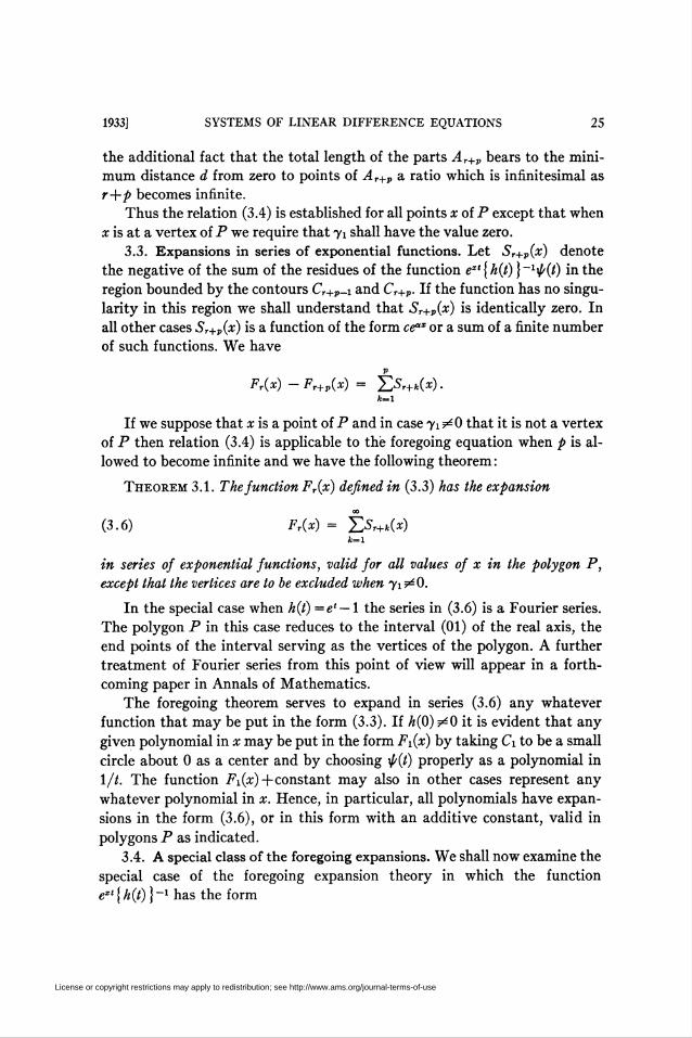
3.3. Expansions in series of exponential functions. Let Sr+P(x) denote
the negative of the sum of the residues of the function ext{h(t) }~1\p(t) in the
region bounded by the contours Cr+P-i and Cr+P. If the function has no singu-
larity in this region we shall understand that Sr+P(x) is identically zero. In
all other cases Sr+P(x) is a function of the form ce"x or a sum of a finite number
of such functions. We have
Fr(x) -Fr+P(x) = ¿Sr+*(x).*=i
If we suppose that x is a point of P and in case 71 ̂ 0 that it is not a vertex
of P then relation (3.4) is applicable to the foregoing equation when p is al-
lowed to become infinite and we have the following theorem :
Theorem 3.1. The function Fr(x) defined in (3.3) has the expansion
(3.6) Fr(x) = jtsr+k(x)k=l
in series of exponential functions, valid for all values of x in the polygon P,
except that the vertices are to be excluded when 71 ̂ 0.
In the special case when h(t) =e' — l the series in (3.6) is a Fourier series.
The polygon P in this case reduces to the interval (01) of the real axis, the
end points of the interval serving as the vertices of the polygon. A further
treatment of Fourier series from this point of view will appear in a forth-
coming paper in Annals of Mathematics.
The foregoing theorem serves to expand in series (3.6) any whatever
function that may be put in the form (3.3). If h(0) ^0 it is evident that any
given polynomial in x may be put in the form Fi(x) by taking Ci to be a small
circle about 0 as a center and by choosing \f/(t) properly as a polynomial in
1/t. The function Fi(x)+ constant may also in other cases represent any
whatever polynomial in x. Hence, in particular, all polynomials have expan-
sions in the form (3.6), or in this form with an additive constant, valid in
polygons P as indicated.
3.4. A special class of the foregoing expansions. We shall now examine the
special case of the foregoing expansion theory in which the function
ex'{ h(t) }_1 has the form
License or copyright restrictions may apply to redistribution; see http://www.ams.org/journal-terms-of-use

26 R. D. CARMICHAEL [January
(e* - l)(e<-* - 1) • • ■ (e'n> - 1) '
where pi, p2, • • • , p„ are n real or complex constants different from 0 and such
that neither the sum nor the difference of two of them is zero.
It is convenient, for the sake of simplicity, to normalize the problem by
means of certain elementary transformations. If pk has a negative real part
we may replace pk by — p* by multiplying both numerator and denominator
in (3.7) by —e~pkt and so obtain (except for an irrelevant change in sign) a
similar expression with x replaced by x— pk', by a translation in the «-plane
we may then replace x—pk by x. We suppose all such translations made so
that we shall assume that the real part of each pk is positive or zero. Then the
further conditions on px, p2, • • • , p„ are that they are different from each
other and from zero. Then the point zero is on the boundary of the polygon P,
introduced (§3.1) in the general case, and the greatest real value of a point in
P is the sum of the real parts of px, p2, • • • , pn. We suppose that the notation
is so chosen that
(3.8) — §r Si arg pi ^ arg p2 ^ • • • ^ arg pn á ¿x.
By means of a straight line join each point (except the last) in the set
, „. 0, pi, Pl + Pi, Pl + Pi + p3, ■ ■ ■ , Pl + Pi + ■ ■ ■ + Pn,(3.9)
Pi + ■ ■ ■ + Pn, ■ ■ ■ , Pn-1 + Pn, Pn, 0
to the one which follows it, thus forming a convex polygon of an even number
of sides and having its sides parallel in pairs. This is the polygon P, as one
sees by examining points x in the sectors formed by adjacent sides. Then the
points x in P ave the points
(3.10) * = XiPi + X2P2+ •••+X„p„ (0¿X»£1;*-1,2, •••,*)»
as one sees by aid of the fact that each of these points lies in the strips each
of which is bounded by two parallel sides of P and by showing that every
point in P is a point x of the named form. The boundary of P is traced out in
counter-clockwise order by starting with all X's equal to zero, then letting
Xi increase from 0 to 1, then X2 from 0 to 1, and so on to X„ letting it increase
from 0 to 1, then letting Xi decrease from 1 to 0, X2 from 1 to 0, and so on till
X„ decreases from 1 to 0.
For every point x in P the function (3.7) may be written in the form
gb-lPlt ^XïM ß^nPn*
License or copyright restrictions may apply to redistribution; see http://www.ams.org/journal-terms-of-use
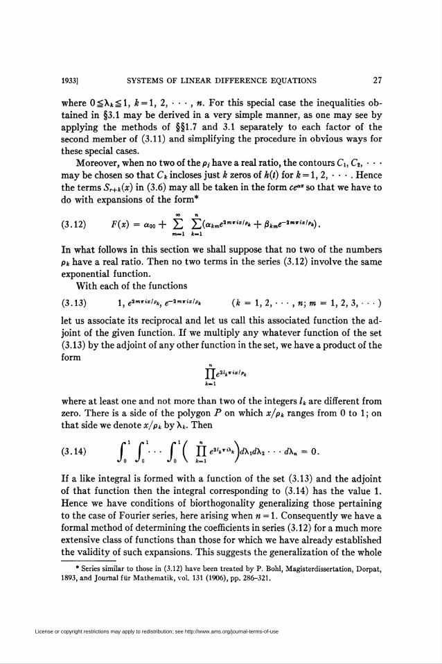
1933] SYSTEMS OF LINEAR DIFFERENCE EQUATIONS 27
where 0=Xt^l, k = l, 2, ■ ■ • , n. For this special case the inequalities ob-
tained in §3.1 may be derived in a very simple manner, as one may see by
applying the methods of §§1.7 and 3.1 separately to each factor of the
second member of (3.11) and simplifying the procedure in obvious ways for
these special cases.
Moreover, when no two of the p,- have a real ratio, the contours G, C2, • • •
may be chosen so that Ck incloses just k zeros of k(t) for k = 1, 2, • • • . Hence
the terms Sr+k(x) in (3.6) may all be taken in the form cc" so that we have to
do with expansions of the form*
oo n
(3.12) F(x) = «oo+E Z(«*m«2mTil/p* + pW-2mTi1'''*).m=l fc=l
In what follows in this section we shall suppose that no two of the numbers
Pk have a real ratio. Then no two terms in the series (3.12) involve the same
exponential function.
With each of the functions
(3.13) 1, e2mrixl>k, e-i™izhk (k = 1,2, ■■■ ,n;m = 1,2,3,- ■ ■)
let us associate its reciprocal and let us call this associated function the ad-
joint of the given function. If we multiply any whatever function of the set
(3.13) by the adjoint of any other function in the set, we have a product of the
formn
rj62¡tT¡z/pt
where at least one and not more than two of the integers h are different from
zero. There is a side of the polygon P on which x/pk ranges from 0 to 1 ; on
that side we denote x/pk by A*. Then
(3.14) f f ■ ■ ■ f ( fi e2lk*ih\d\id\2 ■ ■ ■ d\n = 0.Jo Jo Jo \ A-l /
If a like integral is formed with a function of the set (3.13) and the adjoint
of that function then the integral corresponding to (3.14) has the value 1.
Hence we have conditions of biorthogonality generalizing those pertaining
to the case of Fourier series, here arising when n = 1. Consequently we have a
formal method of determining the coefficients in series (3.12) for a much more
extensive class of functions than those for which we have already established
the validity of such expansions. This suggests the generalization of the whole
* Series similar to those in (3.12) have been treated by P. Bohl, Magisterdissertation, Dorpat,
1893, and Journal für Mathematik, vol. 131 (1906), pp. 286-321.
License or copyright restrictions may apply to redistribution; see http://www.ams.org/journal-terms-of-use

28 R. D. CARMICHAEL
theory of Fourier series to the particular class of series in (3.12) if not indeed
to the more general class of ^3.3; but we shall not now pursue these general-
izations.
Other generalizations of the whole theory developed in this part of the
paper will readily occur to the reader, including among others such exten-
sions of the Birkhoff expansion theory as are parallel to the foregoing exten-
sion of the theory of Fourier series and also the extensions of these theories
to the expansions of functions of several variables; but these also we leave
to a future investigation.
3.5. Applications to Bernoulli polynomials. The theory in §3.4 affords
elegant expansions of Bernoulli polynomials of higher order, namely, the
polynomials B defined by the identity
Pip2 • • • pJnext " /' .
(3.15) PP -P—--= E-£/•>(* pi,---,p„).(gpji _ i) . . . (ep„< _ i) „_0 „|
From this identity we have
,, .,, Rc»>, i v yW« ■■■ Pn r _n^_ dt(3.16) Bv I pi,'". Pn) = - I-
V ' 2xi Jc («*' - 1) • • • («<-' - 1) T+1
where C denotes a small circle about the point zero. Our theory is effective
for values of v not less than ».
Thus we have in particular the expansion
„] " 1 ( e»" g-2*xx gikTix
b;\x\i,í)=- £—\-+-+ (-iy-*--■(27r)-1 t/i k'-1 U»- - 1 e-»* - 1 <r»* - 1
(a.17)
+ ^i^^7Zr1) (, = 3,4,5,...).
According to the general theory this series must converge for those
values x, x = u+iv, for which u and v run independently over the closed
interval (01). By considering separately the four cases u <0, u > 1, v <0, v > 1,
it is easily shown that the series diverges in each case through having terms
in the brackets become infinite in an exponential way as k becomes infinite.
Hence the whole region of convergence of the series is the square whose ver-
tices areO, 1, 1+i, i.
From this example it follows that the polygon P of convergence in the
case of the general theory can not be extended to a larger region in which the
series always converges.
University of Illinois,
Urbana, III.
License or copyright restrictions may apply to redistribution; see http://www.ams.org/journal-terms-of-use