SystemML: Declarative Machine Learning on Spark

Matthias Boehm1, Michael W. Dusenberry2, Deron Eriksson2, Alexandre V.Evfimievski1, Faraz Makari Manshadi1, Niketan Pansare1, Berthold Reinwald1,

Frederick R. Reiss1,2, Prithviraj Sen1, Arvind C. Surve2, Shirish Tatikonda1∗

1 IBM Research – Almaden; San Jose, CA, USA2 IBM Spark Technology Center; San Francisco, CA, USA

ABSTRACTThe rising need for custom machine learning (ML) algo-rithms and the growing data sizes that require the ex-ploitation of distributed, data-parallel frameworks such asMapReduce or Spark, pose significant productivity chal-lenges to data scientists. Apache SystemML addresses thesechallenges through declarative ML by (1) increasing theproductivity of data scientists as they are able to expresscustom algorithms in a familiar domain-specific languagecovering linear algebra primitives and statistical functions,and (2) transparently running these ML algorithms on dis-tributed, data-parallel frameworks by applying cost-basedcompilation techniques to generate efficient, low-level ex-ecution plans with in-memory single-node and large-scaledistributed operations. This paper describes SystemML onApache Spark, end to end, including insights into variousoptimizer and runtime techniques as well as performancecharacteristics. We also share lessons learned from portingSystemML to Spark and declarative ML in general. Finally,SystemML is open-source, which allows the database com-munity to leverage it as a testbed for further research.

1. INTRODUCTIONData scientists are challenged in today’s data economy

due to (1) the need for very sophisticated, custom machinelearning (ML) algorithms—beyond off-the-shelf library al-gorithms, (2) the growing amount of data, partially spurredby the Internet of Things (IoT) in industries such as man-ufacturing, mobile, automotive, and health care, and (3)the resulting need to run these custom ML algorithmson distributed, data-parallel systems such as MapReduce(MR) [14], Spark [41], or Flink [2] for scalability and perfor-mance on cost-efficient commodity clusters.

Overview of SystemML: Apache SystemML [6] ad-dresses these challenges through declarative ML [10] thataims at a high-level specification of ML algorithms to sim-plify the development and deployment of ML algorithmsby separating algorithm semantics from underlying data∗Now at Target Corp.; Work done at IBM Research – Almaden.

This work is licensed under the Creative Commons Attribution-NonCommercial-NoDerivatives 4.0 International License. To view a copyof this license, visit http://creativecommons.org/licenses/by-nc-nd/4.0/. Forany use beyond those covered by this license, obtain permission by emailinginfo@vldb.org.Proceedings of the VLDB Endowment, Vol. 9, No. 13Copyright 2016 VLDB Endowment 2150-8097/16/09.

representations and runtime execution plans. This separa-tion provides tremendous benefits and opportunities, suchas (1) a data-scientist-centric algorithm specification whichimproves the productivity of data scientists, (2) algorithmreusability and simplified deployment for varying data char-acteristics and runtime environments, and (3) automatic op-timization of runtime execution plans. Data scientists ex-press their custom ML algorithms in a domain-specific lan-guage with precise semantics as well as abstract data typesand operations, independent of their implementation. Sys-temML’s language is expressive enough to cover a broadclass of ML algorithms: descriptive statistics, classification,clustering, regression, matrix factorizations, dimensions re-duction, and survival models for training and scoring. Gen-erally, algorithms that can be expressed using vectorizedoperations are a good fit for SystemML. The SystemMLcost-based compiler automatically generates hybrid runtimeexecution plans that are composed of single-node and dis-tributed operations depending on data and cluster charac-teristics such as data size, data sparsity, cluster size, memoryconfigurations, while exploiting the capabilities of underly-ing data-parallel frameworks such as MR or Spark.

SystemML on Spark: SystemML started off with animplementation on MR as the data-parallel framework de-jour [15] in order to share cluster resources with other MR-based systems, and later evolved to utilize the more generalYARN [36]. Apache Spark [5] further offered a number ofadvantages over MR such as a unification of SQL, graph,stream, and ML processing by providing a common RDDdata structure, a general DAG execution engine with lazyevaluation, and distributed in-memory caching. These ca-pabilities make Spark particularly attractive for ML, whichoften requires custom data preparation and repeated, read-only data access in iterative ML algorithms. However, im-plementing ML algorithms directly against Spark compro-mises the benefits of declarative ML and requires substantialeffort. Hence, we decided to fit SystemML into the Sparkecosystem by (1) providing Spark APIs for a seamless in-tegration, and (2) automatically compiling ML algorithmsinto efficient execution plans on top of Spark. DeclarativeML allowed us to transition from MR to YARN and Spark aswell as to support these frameworks simultaneously withoutthe need for any ML algorithm changes.

Contributions: Our major contribution is an end-to-enddescription of declarative ML on Spark. We share lessonslearned, describe implementation choices, introduce severaltechniques that tackle challenges of memory handling andlazy evaluation, and discuss performance insights through

1425

an empirical evaluation of end-to-end ML algorithms. Ourdetailed contributions reflect the structure of this paper:

• Background: We give an up-to-date overview of Sys-temML as a representative system for declarative MLin Section 2, and introduce our running example in thecontext of the SystemML’s Spark APIs.

• Optimizer Integration: We explain optimizer exten-sions for our Spark backend in Section 3. This coversrewrites, memory estimates and constraints, operatorselection, as well as parfor optimizer extensions.

• Runtime Integration: We describe the Spark runtimebackend in Section 4. This includes matrix repre-sentations, the buffer pool integration, partitioning-preserving operations, as well as specific optimizations.

• Experiments: We present end-to-end experimental re-sults for a variety of ML algorithms, data characteris-tics, and spark-specific optimizations in Section 5.

• Discussion and Related Work: Finally, we discusslessons learned from rebasing SystemML on Spark inSection 6, and compare SystemML to related work inthe larger context of large-scale ML in Section 7.

2. BACKGROUNDIn this section, we provide a current overview of Sys-

temML and its high-level architecture with various execu-tion backends, including Spark. We introduce our runningexample in the context of the Spark ecosystem. This exam-ple is used throughout the paper to explain declarative ML,APIs, optimizations, runtime, and performance insights.

2.1 SystemML ArchitectureML algorithms are expressed in a declarative, high-level

language, called DML (Declarative ML). SystemML com-piles and optimizes these algorithms into hybrid runtimeplans of multi-threaded, in-memory operations on a singlenode (scale-up) and distributed MR or Spark operations ona cluster of nodes (scale-out). SystemML’s high-level archi-tecture consists of the following components.

Language: DML (with either R- or Python-like syntax)provides linear algebra primitives, a rich set of statisticalfunctions and matrix manipulations, as well as user-definedand external functions, control structures including parforloops, and recursion [6]. The language component parses agiven DML script into a hierarchy of statement blocks andstatements as defined by control structures, and performssyntactic analysis, live variable analysis, and semantic vali-dation (e.g., matching matrix dimensions). During that pro-cess we also retrieve input data characteristics—i.e., format,number of rows, columns, and non-zero values—as well asinfrastructure characteristics, which are used for subsequentoptimizations. Finally, we construct directed acyclic graphs(DAGs) of high-level operators (HOPs) per statement block.

Optimizer: The SystemML optimizer [8, 9, 19] worksover programs of HOP DAGs, where HOPs are operators onmatrices or scalars, and are categorized according to theiraccess patterns. Examples are matrix multiplications, unaryaggregates like rowSums(), binary operations like cell-wisematrix additions, reorganization operations like transpose orsort, and more specific operations. We perform various opti-mizations on these HOP DAGs, including algebraic simplifi-cation rewrites, intra-/inter-procedural analysis for statistics

propagation into functions and over entire programs, andoperator ordering of matrix multiplication chains. We com-pute memory estimates for all HOPs, reflecting the mem-ory requirements of in-memory single-node operations andintermediates. Each HOP DAG is compiled to a DAG oflow-level operators (LOPs) such as grouping and aggregate,which are backend-specific physical operators. Operator se-lection picks the best physical operators for a given HOPbased on memory estimates, data, and cluster characteris-tics. Individual LOPs have corresponding runtime imple-mentations, called instructions, and the optimizer generatesan executable runtime program of instructions.

Runtime: We execute the generated runtime program lo-cally in CP (control program), i.e., within a driver process.This driver handles recompilation, runs in-memory single-node CP instructions (some of which are multi-threaded),maintains an in-memory buffer pool, and launches MR orSpark jobs if the runtime plan contains distributed compu-tations in the form of MR or Spark instructions [8, 15]. Forthe MR backend, the SystemML compiler groups LOPs—and thus, MR instructions—into a minimal number of MRjobs (MR-job instructions), whereas for the Spark backend,we rely on Spark’s lazy evaluation and stage construction.CP instructions may also be backed by GPU kernels [7].The multi-level buffer pool caches local matrices in-memory,evicts them if necessary, and handles data exchange betweenlocal and distributed runtime backends. Both CP and dis-tributed operations for descriptive statistics and aggrega-tions are numerically stable [35]. The core of SystemML’sruntime instructions is an adaptive matrix block library,which is sparsity-aware and operates on the entire matrixin CP, or blocks of a matrix in a distributed setting. Fur-ther key features include parallel for-loops for task-parallelcomputations [8], and dynamic recompilation for runtimeplan adaptation addressing initial unknowns [9].

2.2 Running ExampleAs our running example, we introduce a DML script of

the popular alternating least squares (ALS) algorithm formatrix completion [43]. In the context of collaborative fil-tering in recommender systems, ALS tries to decomposea partially observed user-item-rating matrix X (m × n)into two factor matrices U (m × r representing user fac-tors) and V (r × n representing item factors) of low rankr � min (m,n), such that X ≈ UV. In our example,the quality of the approximation is measured as L2 reg-ularized squared loss over the observed entries of X withL =

∑i,j Wij(Xij − [UV]ij)

2 + λ(‖U‖2F + ‖V‖2F

), where

‖·‖F is the Frobenius norm and Wij = |sgn Xij |. ALS re-peatedly keeps one of the unknown matrices fixed and opti-mizes the other; when fixing U or V, we obtain a quadraticleast-squares problem, one per row (column) of U (V) witha globally optimal solution. To solve these least-squaresproblems jointly, we use the conjugate gradient method.

Example ALS-CG Script: Below DML script imple-ments the outlined ALS algorithm. It reads an input matrixX (line 1). After initializing the parameters (lines 2-6), wecompute the user and item factors in two nested loops: (1)the outer while loop repeats alternating minimization of fac-tor matrices (U if is U is true, V otherwise) for a fixed numberof iterations mi; (2) the inner while loop performs conjugategradient steps to optimize one of the factor matrices at atime. In R syntax, we write %*% for matrix multiplication

1426

and * for element-wise multiplications. Finally, we outputthe fitted factor matrices U and V (lines 32-33).

1: X = read($inFile);2: r = $rank; lambda = $lambda;3: U = rand(rows=nrow(X), cols=r, min=-1.0, max=1.0);4: V = rand(rows=r, cols=ncol(X), min=-1.0, max=1.0);5: W = (X != 0);6: mi = $maxiter; mii = r; i = 0; is_U = TRUE;7: while(i < mi) {8: i = i + 1; ii = 1;9: if (is_U)

10: G = (W * (U %*% V - X)) %*% t(V) + lambda * U;11: else12: G = t(U) %*% (W * (U %*% V - X)) + lambda * V;13: norm_G2 = sum(G ^ 2); norm_R2 = norm_G2;14: R = -G; S = R;15: while(norm_R2 > 10E-9 * norm_G2 & ii <= mii) {16: if (is_U) {17: HS = (W * (S %*% V)) %*% t(V) + lambda * S;18: alpha = norm_R2 / sum (S * HS);19: U = U + alpha * S;20: } else {21: HS = t(U) %*% (W * (U %*% S)) + lambda * S;22: alpha = norm_R2 / sum (S * HS);23: V = V + alpha * S;24: }25: R = R - alpha * HS;26: old_norm_R2 = norm_R2; norm_R2 = sum(R ^ 2);27: S = R + (norm_R2 / old_norm_R2) * S;28: ii = ii + 1;29: }30: is_U = ! is_U;31: }32: write(U, $outUFile, format = "text");33: write(V, $outVFile, format = "text");

Script Customization: The above DML script uses ma-trix W as an indicator for observed entries in X (line 5). Inother application scenarios, W may represent weights for theentries in X, and may be dense. For example, let W be anouter product of two weight vectors w1 and w2, i.e., W = w1

%*% t(w2). Lines 10, 12, 17, and 21 in the above scriptwould not adequately exploit the modified W, because wecompute U %*% V for every cell where Wij 6= 0. This can becircumvented by applying the following matrix equalities:

# Replace U with S for Line 17(W * (U %*% V)) %*% t(V) = (U*w1) %*% (V*t(w2)) %*% t(V)# Replace V with S for Line 21t(U) %*% (W * (U %*% V)) = t(U) %*% (U*w1) %*% (V*t(w2))

where, for example, U*w1 denotes a matrix-vector element-wise multiplication that logically replicates w1 for every col-umn in U. SystemML is now able to exploit the matrix-product associativity, and order the multiplications in a waythat avoids dense intermediates in the size of X. A data sci-entist may simply apply the outlined changes to customizethe above ALS algorithm to the needs of her application sce-nario, whereas changing a tuned large-scale ALS algorithmimplementation would be a non-trivial endeavor.

MLContext API: SystemML provides an API calledMLContext (in Scala, Java, and Python), that allows theuser to register RDDs and DataFrames (previously createdthrough Spark SQL or other libraries) as input and outputvariables of a DML script. This enables SystemML to seam-lessly integrate into the entire Spark ecosystem. The follow-ing Python example code uses PySpark to read the Movie-Lens dataset to produce and manipulate a Spark DataFrame(lines 2). The MLContext API allows to register and pass the

DataFrame to the ALS algorithm (line 4), invoke the ALSalgorithm with parameters (line 7), get the output factormatrices as DataFrames (lines 8), and invoke a DML scriptfor scoring (line 9, script not shown). We use Spark SQL toperform further data post-processing (lines 12/13).

1: from SystemML import MLContext2: X = csvReader.load("ratings.csv").drop("timestamp")3: ml = MLContext(sc)4: ml.registerInput("X", X)5: ml.registerOutput("U", U)6: ml.registerOutput("V", V)7: outputs = ml.execute("ALS.dml", params)8: U = outputs.getDF(sqlContext, "U") ...9: outputs1 = ml.execute("ALS_predict.dml", params)

10: predictIds = outputs1.getDF("OutP")11: movies = csvReader.load("movies.csv")12: prediction = movies.join(13: predictIds.C1==movies.movieId).select("title")

SystemML provides further APIs, all of which can useexactly the same DML script, which simplifies deployment.

3. OPTIMIZER INTEGRATIONGiven the DML scripts passed in through the various

APIs, SystemML automatically generates efficient executionplans [9]. Optimizer extensions at different levels are re-quired to exploit Spark in a robust and effective way. Inthis section, we describe Spark-specific rewrites, the han-dling of memory budgets and constraints, physical operatorselection, as well as parfor optimizer extensions.

3.1 Spark-Specific RewritesData independence is one of the major goals of declarative

ML [10]. Hence, in contrast to other DSLs [24], SystemMLdoes not expose physical properties like caching and parti-tioning and thus, needs to handle these automatically. Weintroduce Spark-specific rewrites which address decisions ondistributed caching, checkpointing, and partitioning.

Caching/Checkpoint Injection: Spark allows an RDDto be persisted into various storage levels for distributedcaching. We introduce two simple rewrite rules for in-jecting these checkpoints, similar but less aggressive thanin other systems [3]. By default, we use a storage levelMEMORY AND DISK in order to exploit caching without dese-rialization, and to prevent repeated lazy evaluation of ex-pensive operations. First, we inject checkpoints after everypersistent read or reblock (e.g., conversion of text to binaryblock) in order to prevent repeated read from HDFS, textparsing and shuffle. Second, we inject checkpoints beforeloops for all read-only variables in the loop body. Only forparfor loop bodies, checkpoint injection is deferred until par-for optimization. These checkpoints also bring matrices intoread optimized form. We coalesce the number of partitionsaccording to the HDFS block size if necessary. Further, forsparse matrices, we convert matrix blocks into a memory-efficient CSR representation, and for ultra-sparse matrices,we use the storage level MEMORY AND DISK SER if the esti-mated size exceeds the aggregate data memory to preventunnecessary spilling. Finally, as a cleanup step, we removeunnecessary checkpoints: for example, checkpoints in simpleupdate chains or for small datasets that fit into the driver.

Repartition Injection: Operations like join orreduceByKey that cause shuffle are very expensive opera-tions on Spark because shuffle significantly dominates exe-cution time compared to reads from distributed cache. This

1427

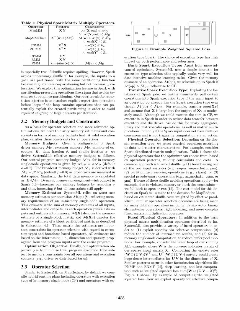
Table 1: Physical Spark Matrix Multiply Operators.Operator Pattern ConstraintsMapMM XY M(X, out) < MB

∨ M(Y, out) < MB

MapMMChain X>(w � (Xv)

)M(w) +M(v) < MB

∧ ncol(X) ≤ Bc

TSMM X>X ncol(X) ≤ Bc

ZIPMM X>Y ncol(X) ≤ Bc

∧ ncol(Y) ≤ Bc

CPMM XY –RMM XY –PMM rmr(diag(v))X M(v) < MB

is especially true if shuffle requires spilling. However, Sparkavoids unnecessary shuffle if, for example, the inputs to ajoin are partitioned with the same partitioning functionbecause it guarantees co-partitioning but not necessarily co-location. We exploit this optimization feature in Spark withpartitioning-preserving operations like zipmm that avoids keychanges to retain co-partitioning. Our rewrite rule for repar-tition injection is to introduce explicit repartition operationsbefore loops if the loop contains operations that can po-tentially exploit the created partitioning in order to avoidrepeated shuffling of large datasets per iteration.

3.2 Memory Budgets and ConstraintsAs a basis for operator selection and more advanced op-

timizations, we need to clarify memory estimates and con-straints in terms of memory budgets first. A valid executionplan, satisfies these constraints for all operations.

Memory Budgets: Given a configuration of Sparkdriver memory MD, executor memory ME, number of ex-ecutors |E|, data fraction δ, and shuffle fraction σ, wederive SystemML’s effective memory budgets as follows.Our control program memory budget MCP for in-memorysingle-node operations is given by MCP = αMD (defaultα=0.7). The broadcast memory budget MB is derived withMB = βδME (default β=0.3) as broadcasts are managed indata space. Similarly, the total data memory is calculatedas |E|δME. Dynamic memory management—introduced inSpark 1.6—increases our memory budgets by removing σand thus, increasing δ but all constraints still apply.

Memory Estimates: SystemML relies on worst-casememory estimates per operationM(op) [8], reflecting mem-ory requirements of an in-memory single-node operation.This estimate is the sum of memory estimates of all inputs,intermediates and outputs, as each operation pins all its in-puts and outputs into memory. M(X) denotes the memoryestimate of a single-block matrix and M(XP) denotes thememory estimate of a block partitioned matrix as describedin Subsection 4.1. These matrix size estimates are impor-tant constraints for operator selection with regard to execu-tion types and broadcast-based operators. All estimates arebased on size information, i.e., dimension and sparsity, prop-agated from the program inputs over the entire program.

Optimization Objective: Finally, our optimization ob-jective φ is to minimize total program execution time sub-ject to memory constraints over all operations and executioncontexts (e.g., driver or distributed tasks).

3.3 Operator SelectionSimilar to SystemML on MapReduce, by default we com-

pile hybrid runtime plans including operators with executiontype of in-memory single-node (CP) and operators with ex-

Figure 1: Example Weighted Squared Loss.

ecution type Spark. The choice of execution type has highimpact on both performance and robustness.

Basic Spark Execution Type: Apart from more ad-vanced optimizers, SystemML uses a simple heuristic forexecution type selection that typically works very well fordata-intensive machine learning tasks. Given the memoryestimate of an operationM(op), we schedule op to Spark ifM(op) > MCP; otherwise to CP.

Transitive Spark Execution Type: Exploiting the lowlatency of Spark jobs, we further transitively pull certainoperations into Spark execution type if the main input toan operation op already has the Spark execution type eventhough M(op) ≤ MCP. For example, consider sum(Xv)and assume that X is large but the output of Xv is moder-ately small. Although we could execute the sum in CP, weexecute it in Spark in order to reduce data transfer betweenexecutors and the driver. We do this for unary aggregates,unary and matrix-scalar operations, as well as matrix multi-plications, but only if the Spark input does not have multipleconsumers and is not triggering computation via an action.

Physical Operator Selection: Depending on the cho-sen execution type, we select physical operators accordingto data and cluster characteristics. For example, considerSpark distributed matrix multiplication. Table 1 shows thephysical operators that the optimizer can choose from, basedon operation patterns, validity constraints and costs. Acommon approach is to avoid shuffle by (1) broadcasting oneof the two input matrices (e.g., mapmm, mapmmchain, pmm),(2) partitioning-preserving operations (e.g., zipmm), or (3)special pseudo-unary operations (e.g., mapmmchain, tsmm, orpmm). If none of these shuffle-avoiding operations apply—forexample, due to violated memory or block size constraints—we fall back to cpmm or rmm [15]. The cost model for this de-cision on Spark is—similar to the decision for MapReduce—based on estimated shuffle costs weighted by effective paral-lelism. Similar operator selection decisions are being madefor many different operators including matrix-vector binaryelement-wise operations, right indexing, and more complexfused matrix multiplication operators.

Fused Physical Operators: In addition to the basicphysical matrix multiplication operators described so far,SystemML also provides a variety of fused operators in or-der to (1) exploit sparsity via selective computation, (2)reduce the number of intermediate results, and (3) for in-memory single-node computation, to reduce buffer pool evic-tions. For example, consider the inner loop of our runningALS example, where W is the non-zero indicator matrix ofour sparse input matrix X. Computing the update rules(W� (U V))V> and U>(W� (U V)) naıvely would createhuge dense intermediates for U V in the dimensions of X.Similar patterns occur in other factorization algorithms likePNMF and ENMF [22], deep learning, and loss computa-tion such as weighted squared loss sum(W � (U V −X)2).Figure 1 shows—by example of computing the weightedsquared loss—how we exploit sparsity for selective compu-

1428

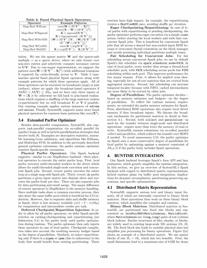
Table 2: Fused Physical Spark Operators.Operator Example Patterns

Map/Red WSLoss sum(W � (UV> −X)2)sum((X−W � (UV>))2)

Map/Red WSigmoid X� sigmoid(UV>)X� log(sigmoid(−(UV>)))

Map/Red WDivMM (W � (UV>))V, (W/(UV>))V(U>(W � (UV>)))>

Map/Red WCeMM sum(X� log(UV>))Map/Red WuMM X� exp(UV>), X/(UV>)2

tation. We use the sparse matrix W and the sparse-safemultiply � as a sparse driver, where we only iterate overnon-zero entries and selectively compute necessary entriesin U V. Due to row-major representation, we support thepattern sum(W� (U V>−X)2) (with additional transposeif required) for cache-friendly access to V. Table 2 sum-marizes special fused physical Spark operators along withexample patterns for which these operators apply. All ofthese operators can be executed via broadcasts (map) or join(reduce), where we apply the broadcast-based operators ifM(U) +M(V) ≤ MB, and we have only three inputs orW = (X 6= 0); otherwise we fall back to join-based realiza-tions which requires a shuffling of the large matrices (unlessco-partitioned) but we still broadcast U or V if possible.Our running example applies various instances of wdivmm

and wsloss. Finally, SystemML supports many more fusedphysical operators for common basic patterns like sum(X2).

3.4 Extended ParFor OptimizerBesides data-parallel computation, SystemML also sup-

ports task-parallel computation via so-called parallel for(parfor) loops as well as hybrid parallelization strategies thatinvolve both [8]. Examples are descriptive statistics, ensem-ble learning/cross validation, and algorithms like KMeans,and Multiclass SVM. In addition to the previously describedgeneral optimizer extensions, the parfor runtime optimizerrequires Spark-specific extensions.

Physical ParFor Operators: Our Spark backendsupports—similar to our MapReduce backend—three phys-ical operators to execute the entire parfor loop. First, localparfor executes multi-threaded workers in the driver whichallows for multi-threaded single-node execution and concur-rent Spark jobs. Second, remote parfor executes the entireloop as a single map-side Spark job. Third, remote dp parforpartitions a given input matrix into disjoint slices and exe-cutes the parfor body per slice. There are also separate jobsfor data partitioning and result merge. The major differenceof remote operators to MapReduce is the memory handling.Since multiple tasks share a common executor process, theyalso share the same buffer pool which is beneficial for I/O re-duction. However, due to separate data and shuffle memoryin Spark, there is less memory available (α(1 − δ − σ)ME)for computation and intermediate results per task.

Deferred Checkpoint/Repartition Injection: In or-der to allow for all parfor operators, we defer Spark-specificrewrites on caching/checkpointing and repartitioning (seeSubsection 3.1) in the parfor body until parfor optimiza-tion during runtime. The parfor optimizer then only injectsthese operators in case of local parfor. Checkpoint compila-tion takes into account the resulting memory budget basedon the degree of parallelism. Similarly, we inject repartition-ing only if there is a zipmm or cpmm (due to unknowns) in thebody that would benefit from existing partitioning. These

rewrites have high impact: for example, the repartitioningcreates a ShuffledRDD once, avoiding shuffle per iteration.

Eager Checkpointing/Repartitioning: In case of lo-cal parfor with repartitioning or pending checkpointing, theparfor optimizer performs eager execution via a simple countaction, before starting the local workers and with that con-current Spark jobs. This is beneficial for concurrent Sparkjobs that all access a shared but non-cached input RDD be-cause it overcomes thread contention on the block managerand avoids persisting individual partitions multiple times.

Fair Scheduling for Concurrent Jobs: For fairscheduling across concurrent Spark jobs, we use by defaultSpark’s fair scheduler via spark.scheduler.mode=FAIR. Incase of local parfor, every worker then setups a thread-localscheduler pool, with FAIR scheduling across pools but FIFO

scheduling within each pool. This improves performance fortwo major reasons. First, it allows for implicit scan shar-ing, especially for out-of-core matrices that are evicted fromaggregated memory. Second, fair scheduling can increasetemporal locality because with FIFO, cached intermediatesare more likely to be evicted by other jobs.

Degree of Parallelism: The parfor optimizer decides—based on memory estimates and budgets—on the degreeof parallelism. To reflect the runtime memory require-ments, we extended the parfor memory estimates for Spark.First, distributed RDD operations also require local drivermemory if they broadcast inputs. We discuss the broad-cast mechanism for partitioned matrices in detail in Sub-section 4.1. Second, both collect and parallelize—asused for the transfer between single-node and distributedoperations—require more than twice the memory of read orwrite. SystemML ensures robustness via so-called guardedcollect and parallelize, which redirect the transfer over HDFSif needed. To avoid unnecessary I/O, the parfor optimizeron Spark uses a more conservative degree of parallelism forlocal parfor by optimizing against a memory constraint ofMCP/2 if the parfor body includes Spark operations.

4. RUNTIME INTEGRATIONOur Spark backend leverages Spark’s Java API and lazy

evaluation, which greatly simplifies the runtime integration.In this section, we give an overview of SystemML’s Sparkbackend with regard to distributed matrix representations,hybrid runtime plans via buffer pool integration, implica-tions for dynamic recompilation, partitioning-preserving op-erations, and specific optimizations.

4.1 Distributed Matrix RepresentationSystemML supports various text and binary input for-

mats, all of which are internally converted to binary blockmatrices. Most operations then work on these binary blockmatrices, which simplifies the compiler and runtime.

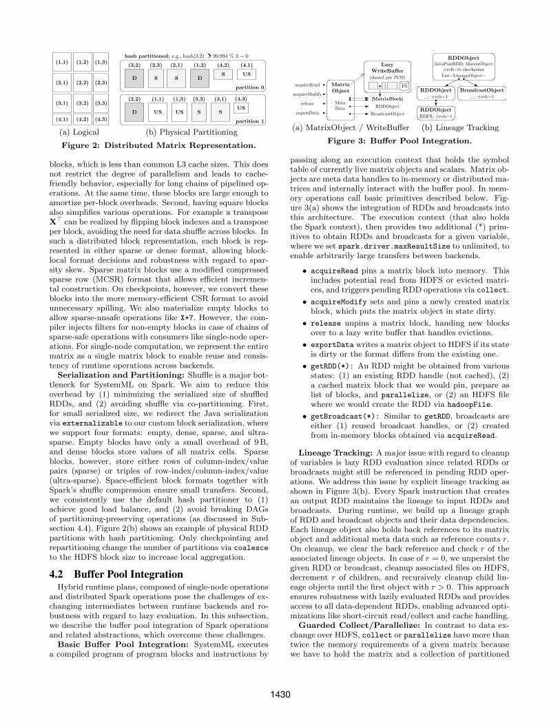
Binary Block Matrices: Distributed matrices in Sys-temML are partitioned into fixed size blocks and rep-resented as JavaPairRDD<MatrixIndexes, MatrixBlock>,where MatrixIndexes are (long,long)-pairs of row/columnblock indexes. Similar structures of tiles, chunks, or blocks,are widely used in existing large-scale ML systems [18, 33,40]. The fixed block size leads to variable physical sizes butsimplifies join processing for binary operations. Figure 2(a)shows an example of a distributed matrix. We use squareblocks of size Bc = 1K, which has two benefits. First, thesmall dimensions lead to a maximum size of 8 MB for dense

1429

(a) Logical

e.g., hash(3,2) 99,994 % 2 = 0

(b) Physical Partitioning

Figure 2: Distributed Matrix Representation.

blocks, which is less than common L3 cache sizes. This doesnot restrict the degree of parallelism and leads to cache-friendly behavior, especially for long chains of pipelined op-erations. At the same time, these blocks are large enough toamortize per-block overheads. Second, having square blocksalso simplifies various operations. For example a transposeX> can be realized by flipping block indexes and a transposeper block, avoiding the need for data shuffle across blocks. Insuch a distributed block representation, each block is rep-resented in either sparse or dense format, allowing block-local format decisions and robustness with regard to spar-sity skew. Sparse matrix blocks use a modified compressedsparse row (MCSR) format that allows efficient incremen-tal construction. On checkpoints, however, we convert theseblocks into the more memory-efficient CSR format to avoidunnecessary spilling. We also materialize empty blocks toallow sparse-unsafe operations like X+7. However, the com-piler injects filters for non-empty blocks in case of chains ofsparse-safe operations with consumers like single-node oper-ations. For single-node computation, we represent the entirematrix as a single matrix block to enable reuse and consis-tency of runtime operations across backends.

Serialization and Partitioning: Shuffle is a major bot-tleneck for SystemML on Spark. We aim to reduce thisoverhead by (1) minimizing the serialized size of shuffledRDDs, and (2) avoiding shuffle via co-partitioning. First,for small serialized size, we redirect the Java serializationvia externalizable to our custom block serialization, wherewe support four formats: empty, dense, sparse, and ultra-sparse. Empty blocks have only a small overhead of 9 B,and dense blocks store values of all matrix cells. Sparseblocks, however, store either rows of column-index/valuepairs (sparse) or triples of row-index/column-index/value(ultra-sparse). Space-efficient block formats together withSpark’s shuffle compression ensure small transfers. Second,we consistently use the default hash partitioner to (1)achieve good load balance, and (2) avoid breaking DAGsof partitioning-preserving operations (as discussed in Sub-section 4.4). Figure 2(b) shows an example of physical RDDpartitions with hash partitioning. Only checkpointing andrepartitioning change the number of partitions via coalesce

to the HDFS block size to increase local aggregation.

4.2 Buffer Pool IntegrationHybrid runtime plans, composed of single-node operations

and distributed Spark operations pose the challenges of ex-changing intermediates between runtime backends and ro-bustness with regard to lazy evaluation. In this subsection,we describe the buffer pool integration of Spark operationsand related abstractions, which overcome these challenges.

Basic Buffer Pool Integration: SystemML executesa compiled program of program blocks and instructions by

acquireRead

acquireModify

release

exportData

[MatrixBlock]RDDObject

BroadcastObject

(shared per JVM)

FS

MetaData

(a) MatrixObject / WriteBuffer

JavaPairRDD; MatrixObject #refs=0; checkpointList<LineageObject>

…; #refs=1 …; #refs=1

HDFS; #refs=1

(b) Lineage Tracking

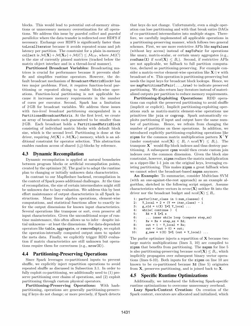
Figure 3: Buffer Pool Integration.

passing along an execution context that holds the symboltable of currently live matrix objects and scalars. Matrix ob-jects are meta data handles to in-memory or distributed ma-trices and internally interact with the buffer pool. In mem-ory operations call basic primitives described below. Fig-ure 3(a) shows the integration of RDDs and broadcasts intothis architecture. The execution context (that also holdsthe Spark context), then provides two additional (*) prim-itives to obtain RDDs and broadcasts for a given variable,where we set spark.driver.maxResultSize to unlimited, toenable arbitrarily large transfers between backends.

• acquireRead pins a matrix block into memory. Thisincludes potential read from HDFS or evicted matri-ces, and triggers pending RDD operations via collect.

• acquireModify sets and pins a newly created matrixblock, which puts the matrix object in state dirty.

• release unpins a matrix block, handing new blocksover to a lazy write buffer that handles evictions.

• exportData writes a matrix object to HDFS if its stateis dirty or the format differs from the existing one.

• getRDD(*): An RDD might be obtained from variousstates: (1) an existing RDD handle (not cached), (2)a cached matrix block that we would pin, prepare aslist of blocks, and parallelize, or (2) an HDFS filewhere we would create the RDD via hadoopFile.

• getBroadcast(*): Similar to getRDD, broadcasts areeither (1) reused broadcast handles, or (2) createdfrom in-memory blocks obtained via acquireRead.

Lineage Tracking: A major issue with regard to cleanupof variables is lazy RDD evaluation since related RDDs orbroadcasts might still be referenced in pending RDD oper-ations. We address this issue by explicit lineage tracking asshown in Figure 3(b). Every Spark instruction that createsan output RDD maintains the lineage to input RDDs andbroadcasts. During runtime, we build up a lineage graphof RDD and broadcast objects and their data dependencies.Each lineage object also holds back references to its matrixobject and additional meta data such as reference counts r.On cleanup, we clear the back reference and check r of theassociated lineage objects. In case of r = 0, we unpersist thegiven RDD or broadcast, cleanup associated files on HDFS,decrement r of children, and recursively cleanup child lin-eage objects until the first object with r > 0. This approachensures robustness with lazily evaluated RDDs and providesaccess to all data-dependent RDDs, enabling advanced opti-mizations like short-circuit read/collect and cache handling.

Guarded Collect/Parallelize: In contrast to data ex-change over HDFS, collect or parallelize have more thantwice the memory requirements of a given matrix becausewe have to hold the matrix and a collection of partitioned

1430

blocks. This would lead to potential out-of-memory situa-tions or unnecessary memory overestimation for all opera-tions. We address this issue by guarded collect and guardedparallelize where the data transfer is redirected over HDFS ifnecessary. Exchange over HDFS is significantly faster thantoLocalIterator because it avoids repeated scans and joblatency per partition. The constraint for a plain in-memorycollect isM(X) +M(XP) +M(C) ≤ MCP, whereM(C)is the size of currently pinned matrices (tracked below thematrix object interface and in a thread-local manner).

Partitioned Broadcast Variables: Broadcasting ma-trices is crucial for performance because it prevents shuf-fle and simplifies runtime operators. However, the de-fault broadcast mechanism of Broadcast<MatrixBlock> hastwo major problems. First, it requires function-local par-titioning or repeated slicing to enable block-wise oper-ations. Function-local partitioning is not applicable be-cause it increases memory requirements in the numberof cores per executor. Second, Spark has a limitationof 2 GB for broadcast variables. We address these issueswith two-level broadcast partitioning encapsulated in aPartitionedBroadcastMatrix. At the first level, we createan array of broadcasts each guaranteed to be smaller than2 GB. Each broadcast holds a PartitionedMatrixBlock

consisting of individual matrix blocks with default blocksize, which is the second level. Partitioning is done at thedriver, requiring M(X) +M(XP) memory, which is an ad-ditional constraint for operator selection. This abstractionenables random access of shared (i,j)-blocks by reference.

4.3 Dynamic RecompilationDynamic recompilation is applied at natural boundaries

between program blocks or artificial recompilation points,created by the optimizer [9]. The goal is to adapt the runtimeplan to changing or initially unknown data characteristics.

In contrast to our MapReduce backend, recompilation inthe context of Spark poses additional challenges. At the timeof recompilation, the size of certain intermediates might stillbe unknown due to lazy evaluation. We address this by besteffort maintenance of output characteristics in all Spark in-structions. Many linear algebra operations, element-wisecomputations, and statistical functions allow to exactly in-fer the output dimensions for known input characteristics.Several operations like transpose or sort, even preserve allinput characteristics. Given the unconditional scope of run-time maintenance, this often allows us to infer—despite ini-tial unknowns—at least the dimensions. For data-dependentoperators like table, aggregate, or removeEmpty, we exploitthe operation-internally computed output sizes to updatethe meta data. Finally, we explicitly trigger RDD evalua-tion if matrix characteristics are still unknown but opera-tions require them for correctness (e.g., nrow(X)).

4.4 Partitioning-Preserving OperationsSince Spark leverages co-partitioned inputs to prevent

shuffle, we explicitly inject repartition operations to avoidrepeated shuffle as discussed in Subsection 3.1. In order tofully exploit co-partitioning, we additionally need to (1) pre-serve partitioning over chains of operations, and (2) exploitpartitioning through custom physical operators.

Partitioning-Preserving Operations: With hash-partitioning, operations are generally partitioning-preserv-ing if keys do not change; or more precisely, if Spark detects

that keys do not change. Unfortunately, even a single oper-ation can lose partitioning and with that break entire DAGsof co-partitioned intermediates into multiple stages. There-fore, we carefully implemented all applicable operations ina partitioning-preserving manner, which follows two generalschemes. First, we use more restrictive APIs like mapValues

(without key access) instead of mapToPair for operationslike unary, matrix-scalar, or certain unary aggregates (e.g.,rowSums(X) if ncol(X) ≤ Bc). Second, if restrictive APIsare not applicable, we fallback to full partition computa-tion, declared as partitioning-preserving. For example con-sider a matrix-vector element-wise operation like X�v withbroadcast of v. This operation is partitioning-preserving butneeds the input keys for broadcast block lookups. Hence, weuse mapPartitionsToPair(...,true) to indicate preservedpartitioning. We also return lazy iterators instead of materi-alized outputs per partition to reduce memory requirements.

Partitioning-Exploiting Operations: RDD opera-tions can exploit the preserved partitioning to avoid shuffle(implicit or explicit). Implicit partitioning-exploiting oper-ations such as matrix-matrix element-wise operations useprimitives like join or cogroup. Spark automatically ex-ploits partitioning if input and output have the same num-ber of partitions. Hence, we refrain from changing thenumber of partitions on these operations. In addition, weintroduced explicitly partitioning-exploiting operations likezipmm for the common matrix multiplication pattern X>Y(under constraint ncol(X) ≤ Bc ∧ ncol(Y) ≤ Bc). Thetranspose X> would flip block indexes and thus destroy par-titioning. A subsequent cpmm would then create custom joinindexes over the common dimension. Given the block sizeconstraint, however, zipmm realizes the matrix multiplicationas a zipper-like 1-1 join on the original keys, leveraging ex-isting partitioning. This makes zipmm a great fallback whenwe cannot select the broadcast-based mapmm anymore.

An Example: To summarize, consider Multiclass SVM(with an one-against-the-rest approach) as an example al-gorithm, sketched in the following script snippet. Assumecharacteristics where vectors in nrow(X) neither fit into thedriver nor the broadcast budget and ncol(X) ≤ Bc.

1: parfor(iter_class in 1:num_classes) {2: Y_local = 2 * (Y == iter_class) - 13: g_old = t(X) %*% Y_local ...4: while( continue ) {5: Xd = X %*% s6: ... inner while loop (compute step_sz)7: Xw = Xw + step_sz * Xd;8: out = 1 - Y_local * Xw;9: out = (out > 0) * out;

10: g_new = t(X) %*% (out * Y_local) ...

The parfor optimizer injects a repartition of X because twolarge matrix multiplications (lines 3, 10) are compiled tozipmm that benefits from partitioning. The mapmm for line 5is also partitioning-preserving because ncol(X) ≤ Bc, whichimplicitly propagates over subsequent binary vector opera-tions (lines 6-10). Both inputs for the zipmm on line 10 areknown to be co-partitioned because Xd (line 5) originatesfrom X, preserves partitioning, and is joined back to X.

4.5 Specific Runtime OptimizationsAdditionally, we introduced the following Spark-specific

runtime optimizations to overcome unnecessary overhead.Lazy Spark-Context Creation: On creation of the

Spark context, executors are allocated and initialized, which

1431

can take up to 20 s. With hybrid runtime plans, this causeslarge unnecessary overhead if all operations are single-nodeoperations that execute in a few seconds. Hence, we lazily al-locate the context on demand when it is first accessed (e.g.,when creating an RDD), which avoids context creation forpure single-node computation. Also, for EXPLAIN and pro-grams with initial unknowns, we defer the access to the con-text (e.g., for memory budgets) as long as possible.

Short-Circuit Read: Due to conservative checkpointcompilation, a single-node operation might directly consumea cached RDD, which causes unnecessary overhead for read-ing the matrix into distributed memory and transfering itback to the driver via collect. Our short-circuit read by-passes the checkpoint based on lineage information and di-rectly reads the matrix from HDFS into the driver.

Short-Circuit Collect: Our short-circuit collect gener-alized upon the concept of short-circuit read, and bypassesRDD caching, if the given RDD is marked for caching butnot yet actually cached. Avoiding caching reduces the over-head of unnecessary reads and memory pressure.

5. EXPERIMENTSWe study end-to-end performance characteristics of Sys-

temML on Spark over a variety of ML algorithms and datacharacteristics as well as specific optimization techniques.

5.1 Experimental SettingCluster Setup: We ran all experiments on a 1+6 node

cluster, i.e., one head node of 2x4 Intel E5530 @ 2.40 GHz-2.66 GHz with hyper-threading enabled and 64 GB RAM,as well as 6 nodes of 2x6 Intel E5-2440 @ 2.40 GHz-2.90 GHz with hyper-threading enabled, 96 GB DDR3RAM @1.33 GHz, 12x2 TB disks, 10Gb Ethernet, and Cen-tOS Linux 7.1. As the runtime environment, we used Open-JDK 1.8.0 65 64bit, Hadoop 2.7.0, Spark 1.5.2, and Sys-temML as of 02/2016. We ran Spark in yarn-client modefrom the head node, with 6 executors, 20 GB driver mem-ory, 55 GB executor memory, and 24 cores per executor. Formap/reduce tasks, we configured a maximum heap size of1.6 GB (2 GB container size) and 384 MB sort buffer. Fi-nally, SystemML’s memory budget ratio was α = 0.7.

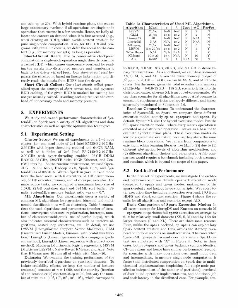
ML Algorithms: Our experiments cover a variety ofcommon ML algorithms for regression, binomial and multi-nomial classification, as well as clustering. Table 3 summa-rizes the used algorithms and parameters (number of itera-tions, convergence tolerance, regularization, intercept, num-ber of classes/centroids/rank, use of parfor loops), whichalso indicates essential characteristics such as iterative al-gorithms, nested loop structures, etc. In detail, we useL2SVM (L2-regularized Support Vector Machines), GLM(Generalized Linear Models, binomial with probit link func-tion), LinregCG (Linear regression with a conjugate gradi-ent method), LinregDS (Linear regression with a direct solvemethod), MLogreg (Multinomial logistic regression), MSVM(Multiclass L2SVM), Naıve Bayes, KMeans, and ALS. Notethat KMeans uses 10 runs all of which with Maxi=20.

Datasets: We evaluate the training performance of thepreviously described algorithms on synthetic datasets. Toisolate scalability effects, we keep the number of features(columns) constant at n = 1,000, and the sparsity (fractionof non-zeros to cells) constant at sp = 0.9, but vary the num-ber of rows m ∈ {104, 105, 106, 107, 108}, which corresponds

Table 3: Characteristics of Used ML Algorithms.Algorithm Maxi ε λ Icpt #C ParFor

L2SVM 20/∞ 1e-6 1e-2 N 2 NGLM 20/∞ 1e-6 1e-2 N 2 N

LinregCG 20 1e-6 1e-2 N N/A NLinregDS N/A N/A 1e-2 N N/A NMLogreg 20/∞ 1e-6 1e-2 N 5 NMSVM 5× 20/∞ 1e-6 1e-2 N 5 Y

Naıve Bayes N/A N/A N/A N 5 YKMeans 10× 20 1e-4 N/A N 10 Y

ALS 6/50* 0 1 N/A 50 N

to 80 MB, 800 MB, 8 GB, 80 GB, and 800 GB in dense bi-nary representation. As a shorthand, we call these scenariosXS, S, M, L, and XL. Given the driver memory budget ofMCP = α ·20 GB = 14 GB, we can fit XS, S, and M into thedriver. Furthermore, given the total executor data memoryof |E|δME = 6·0.6·55 GB = 198 GB, scenario L fits into thedistributed cache, whereas XL is an out-of-core scenario. Weuse these scenarios for all algorithms except ALS because itscommon data characteristics are largely different and hence,separately introduced in Subsection 5.6.

Baseline Comparisons: To understand the character-istics of SystemML on Spark, we compare three differentexecution modes, namely cp+mr, cp+spark, and spark. Bydefault, SystemML uses the hybrid execution modes, but thefull spark execution mode—where every matrix operation isexecuted as a distributed operation—serves as a baseline toevaluate hybrid runtime plans. These execution modes al-low for a systematic evaluation because they share the sameruntime block operations. We refrain from comparisons toexisting machine learning libraries like MLlib [25] due to (1)different abstraction levels of algorithm specification, and(2) different algorithm choices and parameters. A fair com-parison would require a benchmark including both accuracyand runtime, which is beyond the scope of this paper.

5.2 End-to-End PerformanceIn the first set of experiments, we investigate the end-to-

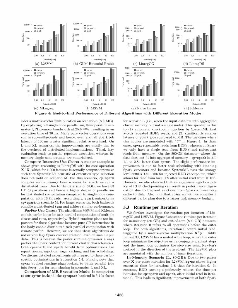
end performance of our default cp+spark execution modecompared to spark and cp+mr modes, making use of thespark-submit and hadoop invocation scripts. We report to-tal execution time including invocation overhead, I/O fromHDFS and Spark context creation. Figure 4 shows the re-sults for all algorithms and scenarios except ALS.

Basic Comparison of Spark Execution Modes: Inall cases—except for LinregDS and Kmeans on scenario M—cp+spark outperforms full spark execution on average by6.1x for relatively small datasets (XS, S, M) and by 1.9x forlarger datasets (L and XL). There are three main reasons.First, unlike the spark backend, cp+spark can exploit lazySpark context creation and thus, avoids the start-up over-head of up to 20 seconds on small scenarios. The cases whenSystemML cp+spark backend does not create a SparkCon-text are annotated with “X” in Figure 4. Note, in thesecases, both cp+spark and cp+mr backends compile identicalCP-only plans and hence have similar performance. Second,for scenarios with many operations over small input dataand intermediates, in-memory single-node computation isfaster than distributed computation on Spark due to multi-threaded implementations (exploiting full single-node par-allelism independent of the number of partitions), overheadof distributed operator implementations, and additional joband task latency in the distributed case. For example, con-

1432

0.08 0.8 8 80 800

cp+mrcp+sparkspark

1

10

100

1000

10000Ti

me

[sec

]

Data size [GB]

XX

X

Y

(a) L2SVM

0.08 0.8 8 80 800

cp+mrcp+sparkspark

1

10

100

1000

10000

100000

Tim

e [s

ec]

Data size [GB]

X XX

Y

(b) GLM Binomial Probit

0.08 0.8 8 80 800

cp+mrcp+sparkspark

1

510

50100

5001000

Tim

e [s

ec]

Data size [GB]

XX

X

Y

(c) LinregCG

0.08 0.8 8 80 800

cp+mrcp+sparkspark

1

510

50100

5001000

Tim

e [s

ec]

Data size [GB]

XX

XY

(d) LinregDS

0.08 0.8 8 80 800

cp+mrcp+sparkspark

1

10

100

1000

10000

100000

Tim

e [s

ec]

Data size [GB]

X X

X

Y

(e) MLogreg

0.08 0.8 8 80 800

cp+mrcp+sparkspark

1

10

100

1000

10000Ti

me

[sec

]

Data size [GB]

Y

(f) MSVM

0.08 0.8 8 80 800

cp+mrcp+sparkspark

1

510

50100

5001000

5000

Tim

e [s

ec]

Data size [GB]

X XX

Y

(g) Naıve Bayes

0.08 0.8 8 80 800

cp+mrcp+sparkspark

1

10

100

1000

10000

Tim

e [s

ec]

Data size [GB]

Y

(h) KMeans

Figure 4: End-to-End Performance of Different Algorithms with Different Execution Modes.

sider a matrix-vector multiplication on scenario S (800 MB).By exploiting full single-node parallelism, this operation sat-urates QPI memory bandwidth at 25.6 GB/s, resulting in anexecution time of 30 ms. Many pure vector operations evenrun in sub-milliseconds and hence, even a small Spark joblatency of 100 ms creates significant relative overhead. OnL and XL scenarios, the improvements are mostly due tothe overhead of distributed implementations. Third, lazyevaluation leads to partial repeated execution, whereas in-memory single-node outputs are materialized.

Compute-Intensive Use Cases: A counter example toabove given reasoning is LinregDS with its core operationX>X, which for 1,000 features is actually compute-intensivesuch that SystemML’s heuristic of execution type selectiondoes not hold on scenario M. For this scenario, cp+spark

compiles an in-memory tsmm whereas for spark we run adistributed tsmm. Due to the data size of 8 GB, we have 63HDFS partitions and hence a higher degree of parallelismfor distributed computation compared to single-node com-putation with 16 threads. Accordingly, spark outperformscp+spark on scenario M. For larger scenarios, both backendscompile a distributed tsmm and achieve similar performance.

ParFor Use Cases: The algorithms MSVM and KMeansexploit parfor loops for task-parallel computation of multipleclasses and runs, respectively. Hybrid runtime plans are im-portant for these algorithms because pure CP instructions inthe body enable distributed task-parallel computation withremote parfor. However, we see that these algorithms donot exploit lazy Spark context creation, even on small inputdata. This is because the parfor runtime optimizer alwaysprobes the Spark context for current cluster characteristics.Both cp+spark and spark benefit from optimizations likerepartitioning injection, eager caching, and fair scheduling.We discuss detailed experiments with regard to these parfor-specific optimizations in Subsection 5.4. Finally, note thatcp+mr applied runtime piggybacking to batch parallel jobsinto fewer jobs for scan sharing in scenarios L and XL.

Comparison of MR Execution Mode: In comparisonto our cp+mr backend, the cp+spark backend is 5-10x faster

for scenario L (i.e., when the input data fits into aggregatedcluster memory but not a single node). This speedup is dueto (1) automatic checkpoint injection by SystemML thatavoids repeated HDFS reads, and (2) significantly smallerlatency of Spark jobs compared to MR. The use cases wherethis applies are annotated with “Y” in Figure 4. In thesecases, cp+mr repeatably reads from HDFS, whereas on Sparkwe only have a single read from HDFS and subsequentreads from memory. On the 800 GB datasets—where thedata does not fit into aggregated memory—cp+spark is still1.1 to 2.8x faster than cp+mr. The slight performance im-provement is due to faster task scheduling with standingSpark executors and because SystemML uses the storagelevel MEMORY AND DISK for injected RDD checkpoints, whichallows for read from local FS after initial read from HDFS.However, we also observed that an aggressive injection pol-icy of RDD checkpointing can result in performance degra-dation due to frequent evictions from Spark’s in-memorycache to disk. Also note that cp+mr sometimes compiles adifferent parfor plan due to a larger task memory budget.

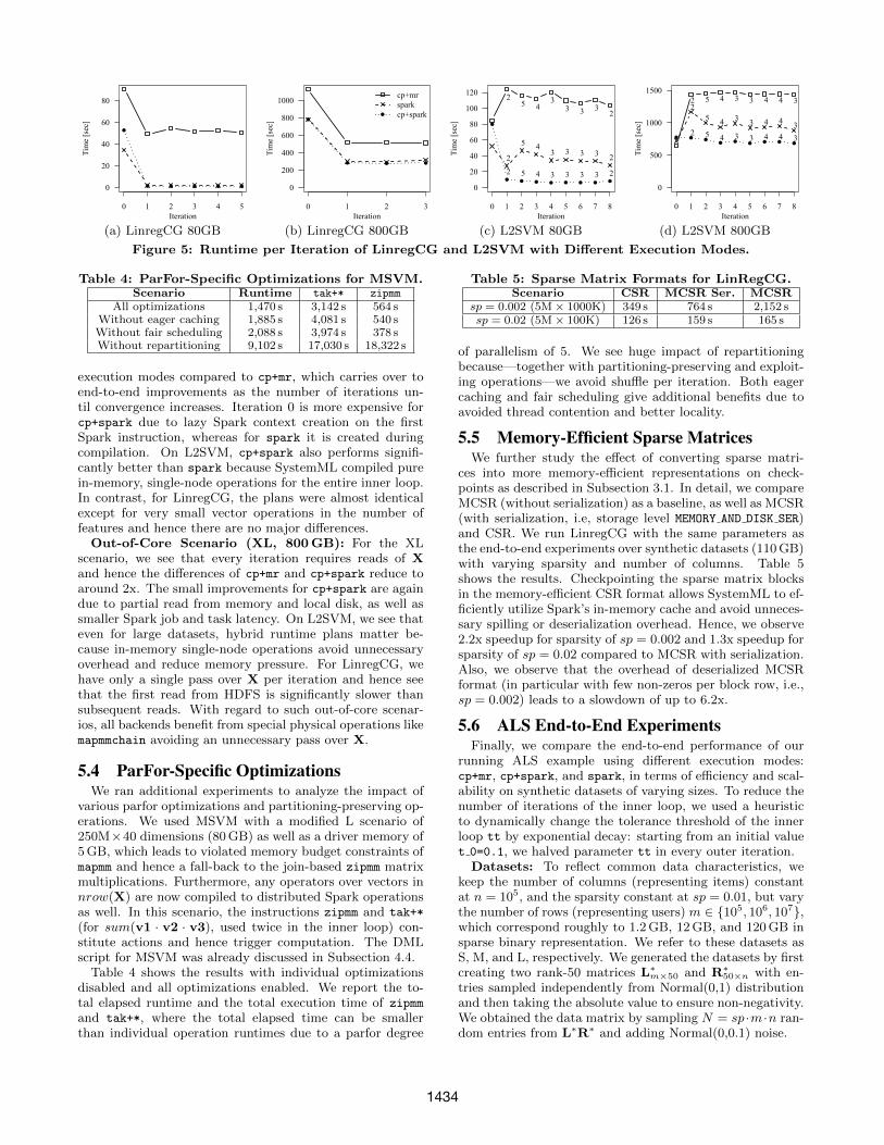
5.3 Runtime per IterationWe further investigate the runtime per iteration of Lin-

regCG and L2SVM. Figure 5 shows the runtime per iterationfor in-memory (80 GB) and out-of-core (800 GB) datasets,where iteration 0 refers to all operations before the outerloop. For both algorithms, iteration 0 covers initial read,triggered by a matrix-vector multiplication X>y. UnlikeLinregCG, L2SVM has a nested while loop, where the outerloop minimizes the objective using conjugate gradient stepsand the inner loop optimizes the step size using Newton’smethod in the direction of the gradient. The L2SVM plotsare annotated with the number of inner iterations.

In-Memory Scenario (L, 80 GB): Due to two passesover X per outer iteration for L2SVM, cp+mr shows higherexecution time for iterations 1-8 than for iteration 0. Incontrast, RDD caching significantly reduces the time periteration for cp+spark and spark, after initial read in itera-tion 0. This leads to significant improvements of both Spark

1433

0

20

40

60

80

0 1 2 3 4 5

Tim

e [s

ec]

Iteration

●

● ● ● ● ●

(a) LinregCG 80GB

0

200

400

600

800

1000

0 1 2 3

Tim

e [s

ec]

Iteration

●

● ● ●

●

cp+mrsparkcp+spark

(b) LinregCG 800GB

0

20

40

60

80

100

120

0 1 2 3 4 5 6 7 8

Tim

e [s

ec]

Iteration

25 4

33 3 3

2

2

5 43 3 3 3 2

●

● ● ● ● ● ● ● ●

2 5 4 3 3 3 3 2

(c) L2SVM 80GB

�

���

����

����

� � � � � � �

�� �������

���������

� � � � � � � ��

� � � � � � �● ● ●

● ● ● ● ● ●

� � � � � � � �

(d) L2SVM 800GB

Figure 5: Runtime per Iteration of LinregCG and L2SVM with Different Execution Modes.

Table 4: ParFor-Specific Optimizations for MSVM.Scenario Runtime tak+* zipmm

All optimizations 1,470 s 3,142 s 564 sWithout eager caching 1,885 s 4,081 s 540 sWithout fair scheduling 2,088 s 3,974 s 378 sWithout repartitioning 9,102 s 17,030 s 18,322 s

execution modes compared to cp+mr, which carries over toend-to-end improvements as the number of iterations un-til convergence increases. Iteration 0 is more expensive forcp+spark due to lazy Spark context creation on the firstSpark instruction, whereas for spark it is created duringcompilation. On L2SVM, cp+spark also performs signifi-cantly better than spark because SystemML compiled purein-memory, single-node operations for the entire inner loop.In contrast, for LinregCG, the plans were almost identicalexcept for very small vector operations in the number offeatures and hence there are no major differences.

Out-of-Core Scenario (XL, 800 GB): For the XLscenario, we see that every iteration requires reads of Xand hence the differences of cp+mr and cp+spark reduce toaround 2x. The small improvements for cp+spark are againdue to partial read from memory and local disk, as well assmaller Spark job and task latency. On L2SVM, we see thateven for large datasets, hybrid runtime plans matter be-cause in-memory single-node operations avoid unnecessaryoverhead and reduce memory pressure. For LinregCG, wehave only a single pass over X per iteration and hence seethat the first read from HDFS is significantly slower thansubsequent reads. With regard to such out-of-core scenar-ios, all backends benefit from special physical operations likemapmmchain avoiding an unnecessary pass over X.

5.4 ParFor-Specific OptimizationsWe ran additional experiments to analyze the impact of

various parfor optimizations and partitioning-preserving op-erations. We used MSVM with a modified L scenario of250M×40 dimensions (80 GB) as well as a driver memory of5 GB, which leads to violated memory budget constraints ofmapmm and hence a fall-back to the join-based zipmm matrixmultiplications. Furthermore, any operators over vectors innrow(X) are now compiled to distributed Spark operationsas well. In this scenario, the instructions zipmm and tak+*

(for sum(v1 · v2 · v3), used twice in the inner loop) con-stitute actions and hence trigger computation. The DMLscript for MSVM was already discussed in Subsection 4.4.

Table 4 shows the results with individual optimizationsdisabled and all optimizations enabled. We report the to-tal elapsed runtime and the total execution time of zipmm

and tak+*, where the total elapsed time can be smallerthan individual operation runtimes due to a parfor degree

Table 5: Sparse Matrix Formats for LinRegCG.Scenario CSR MCSR Ser. MCSR

sp = 0.002 (5M× 1000K) 349 s 764 s 2,152 ssp = 0.02 (5M× 100K) 126 s 159 s 165 s

of parallelism of 5. We see huge impact of repartitioningbecause—together with partitioning-preserving and exploit-ing operations—we avoid shuffle per iteration. Both eagercaching and fair scheduling give additional benefits due toavoided thread contention and better locality.

5.5 Memory-Efficient Sparse MatricesWe further study the effect of converting sparse matri-

ces into more memory-efficient representations on check-points as described in Subsection 3.1. In detail, we compareMCSR (without serialization) as a baseline, as well as MCSR(with serialization, i.e, storage level MEMORY AND DISK SER)and CSR. We run LinregCG with the same parameters asthe end-to-end experiments over synthetic datasets (110 GB)with varying sparsity and number of columns. Table 5shows the results. Checkpointing the sparse matrix blocksin the memory-efficient CSR format allows SystemML to ef-ficiently utilize Spark’s in-memory cache and avoid unneces-sary spilling or deserialization overhead. Hence, we observe2.2x speedup for sparsity of sp = 0.002 and 1.3x speedup forsparsity of sp = 0.02 compared to MCSR with serialization.Also, we observe that the overhead of deserialized MCSRformat (in particular with few non-zeros per block row, i.e.,sp = 0.002) leads to a slowdown of up to 6.2x.

5.6 ALS End-to-End ExperimentsFinally, we compare the end-to-end performance of our

running ALS example using different execution modes:cp+mr, cp+spark, and spark, in terms of efficiency and scal-ability on synthetic datasets of varying sizes. To reduce thenumber of iterations of the inner loop, we used a heuristicto dynamically change the tolerance threshold of the innerloop tt by exponential decay: starting from an initial valuet 0=0.1, we halved parameter tt in every outer iteration.

Datasets: To reflect common data characteristics, wekeep the number of columns (representing items) constantat n = 105, and the sparsity constant at sp = 0.01, but varythe number of rows (representing users) m ∈ {105, 106, 107},which correspond roughly to 1.2 GB, 12 GB, and 120 GB insparse binary representation. We refer to these datasets asS, M, and L, respectively. We generated the datasets by firstcreating two rank-50 matrices L∗m×50 and R∗50×n with en-tries sampled independently from Normal(0,1) distributionand then taking the absolute value to ensure non-negativity.We obtained the data matrix by sampling N = sp ·m ·n ran-dom entries from L∗R∗ and adding Normal(0,0.1) noise.

1434

Table 6: ALS End-to-End Performance.Scenario cp+mr cp+spark spark

S (105 × 105, 0.01, 1.2 GB) 131 s 136 s 135 sM (106 × 105, 0.01, 12 GB) 1,088 s 342 s 432 sL (107 × 105, 0.01, 120 GB) >24 h 10,537 s 15,487 s

Setup: We used the same configuration as described inSection 5.1 across all execution modes, except for a drivermemory of 15 GB for the S and M dataset and 30 GB for theL dataset. In our experiments, we compute a rank r = 50factorization by minimizing the L2 regularized squared losswith the regularization parameter λ = 1.0 throughout. Ineach case, we ran the ALS algorithm for 6 iterations.

Comparison Results: Table 6 summarizes the resultsof the end-to-end runtime comparison (including the timeto read the input matrix, fitting the model, and writing thecomputed factor matrices) of ALS for all three executionmodes. We see that running ALS on cp+spark is clearlybeneficial across all datasets. On the S dataset, all threeexecution modes perform similar, even though ALS withcp+mr or cp+spark run purely in CP mode (multi-threadedon the head node), whereas ALS with spark utilizes all thecluster nodes. For the larger M and L scenarios, however,the cp+spark generates hybrid execution plans including CPand Spark instructions and outperforms the other execu-tion modes. ALS in cp+mr did not terminate within 24 h ondataset L, since the user-factors (matrix U in our runningexample from Subsection 2.2) did not fit into the memoryof map/reduce tasks. Consequently, replication and shuf-fling led to repeated spilling. In contrast, both spark andcp+spark execution modes generated broadcast-based oper-ators as U is shared across executor cores.

6. DISCUSSIONFinally, we share major lessons learned with regard to Sys-

temML on top of Spark, but also declarative ML in general.Spark over Custom Framework: SystemML on MR

was motivated by sharing cluster resources with other MR-based systems. With YARN things changed as it enablesmulti-tenancy across frameworks. Before deciding for aSpark backend, we discussed alternatives including a customframework implemented from scratch. Eventually we havechosen Spark, not just because it is a well-engineered frame-work with strong contributor base, but mostly to provideusers the flexibility of seamless data preparation and featureengineering, which is invaluable for end-to-end pipelines.

Stateful Distributed Caching: The ability to exploitdistributed caching (of deserialized objects) via standingexecutors together with Spark’s fast task scheduling reallymade a performance difference for SystemML. However, italso came with challenges like (1) reduced working memoryfor task-parallel computation, (2) state-dependent memoryconstraints, (3) global effects of update-in-place, and (4) fairresource management in shared clusters.

Memory-Efficiency: In contrast to SystemML on MR,where we process one block at-a-time, memory-efficiency isfar more important on Spark to avoid unnecessary cachespilling. Examples of how to reduce memory pressureare custom serialization via externalizable, compact datastructures for sparse, read-only matrices (e.g., CSR format),and lazy iterators for partition-wise execution.

Lazy RDD Evaluation: Some major advantages butalso challenges of SystemML’s Spark backend were related

to lazy evaluation. First, lazy evaluation removed the needfor custom piggybacking, i.e., grouping distributed opera-tions into jobs for scan sharing. Job execution based on ac-tions usually works very well, except special cases where (1)separate actions trigger multiple passes over a shared input,or (2) complex DAG structures cause repeated execution ofcompute-intensive operations. Second, lazy evaluation alsomade the execution of compiled runtime plans more diffi-cult. Examples are variable cleanup, driver memory man-agement, statistics profiling, runtime plan cost estimation,and dynamic recompilation. Third, lazy evaluation allowsto exploit meta data information of inputs such as existingpartitioning, which was highly beneficial for SystemML.

Declarative ML: Creating the Spark backend also madea great case for declarative ML in general. Data inde-pendence of ML algorithms allowed us to leverage RDDsand related operations without changing a single algorithm.Similarly, we were able to automatically exploit distributedcaching and partitioning by newly introduced Spark-specificrewrites. The separation of concerns between ML algorithmsemantics as well as underlying data structures and execu-tion plan generation also ensures independence of runtimeframeworks like MapReduce or Spark. This independenceallowed us to adapt to new technology like Spark yet main-taining support for MapReduce v1, which overall protectsinvestments in created custom ML algorithms.

7. RELATED WORKWe review related work with regard to alternative speci-

fications and implementations of large-scale ML algorithms.Low-Level Primitives: Beside data-parallel frame-

works like MapReduce [14], Spark [41], or Flink [2], thereexist frameworks that provide low-level distributed primi-tives for ML algorithms. For instance, R’s rmr [27] packageexposes map and reduce primitives, HP’s Distributed R [37]package supports operations on distributed arrays, andREEF [38] provides a scheduler framework designed for ML-specific iterative task life-cycle management on YARN. Fur-thermore, graph processing systems like GraphLab [23] oftenprovide vertex-centric abstractions for graph-parallel oper-ations. Users of these frameworks are burdened with thetasks of devising distributed runtime plans, and optimizingthem for performance and scalability.

ML Libraries: A common approach to large-scale MLis to provide pre-canned distributed implementations of se-lected ML algorithms as libraries. Examples include Ma-hout [4], Spark MLlib [25], MADlib [17], Vowpal Wab-bit [21], Revolution R ScaleR [28], SkyTree ML software [29],and H2O [16]. Such fixed implementations do not fit all sce-narios, cannot be adapted to changing data properties, anddo not allow for algorithm customizations without modify-ing the distributed algorithm implementation.

ML UDF-Centric Systems: At a slightly higher ab-straction level, there are frameworks that provide userswith building blocks and UDF support to construct MLmodels. Examples are TensorFlow [1] that executes dataflow graphs of black-box kernels, DMTK [26] that pro-vides a parameter-server-based framework, MLI [31], ML-PACK [13], Shogun [30], Tupleware [12], and Emma [3].These systems, however, only provide limited automatic op-timization of runtime plans and/or data independence.

Declarative ML: Systems for declarative ML can beclassified into declarative ML algorithms and declarative ML

1435

tasks [10]. Example systems aiming for declarative ML al-gorithms are OptiML [34], SystemML [15], SimSQL [11],SciDB [33], Cumulon [18], DMac [39], and Mahout Samsara[24]. These systems provide a simple yet flexible specifica-tion of ML algorithms, and some of them data independence,and automatic optimization and parallelization. Similar toSystemML, DMac and Mahout Samsara also leverage Sparkfor distributed operations. Frameworks like MLBase [20,32] or Columbus [42] further enable declarative ML tasks ofmodel or feature selection, where they optimize both modelaccuracy and performance of ML algorithms.

8. CONCLUSIONSIn this paper, we have presented an up-to-date overview

of SystemML, necessary engine extensions to deeply ex-ploit Spark, and solutions to unique implementation chal-lenges on Spark such as memory handling and lazy evalua-tion. Spark-specific key optimizations are automatic injec-tion of RDD caching/checkpointing and repartitioning, aswell as partitioning-preserving operations to minimize thenumber of data scans and shuffles. We use fair schedul-ing of concurrent Spark jobs issued from multiple parforthreads. Our Spark backend leverages Spark’s Java API andlazy evaluation. We also explained our distributed matrixrepresentation in RDDs, explicit lineage tracking for robustcleanup of broadcast and RDD variables, explicit triggeringof RDD evaluations for eager caching and repartitioning,dynamic recompilation as well as careful implementation ofpartitioning-preserving and exploiting operations. Our ex-periments show that hybrid execution plans are crucial forperformance, and when compared to MR backend, our Sparkbackend provides up to 5-10x speedup when the data fits inmemory and up to 2x improvement for datasets larger thanthe aggregated memory. We also want to note that the richSpark API significantly simplified the backend implementa-tion for Spark compared to MR. SystemML is open source,and we welcome community contributions.

Acknowledgments: We thank Nakul Jindal, Christian R.Kadner, Jihyoung Kim, Narine Kokhlikyan, Deepak Kumar,Min Li, Luciano Resende, Alok Singh, Glenn Weidner, andWen Pei Yu for their significant contributions to SystemML.

9. REFERENCES[1] M. Abadi et al. TensorFlow: Large-Scale Machine Learning

on Heterogeneous Distributed Systems. CoRR,abs/1603.04467, 2016.

[2] A. Alexandrov et al. The Stratosphere Platform for BigData Analytics. VLDB J., 23(6), 2014.

[3] A. Alexandrov et al. Implicit Parallelism through DeepLanguage Embedding. In SIGMOD, 2015.

[4] Apache. Mahout, 2016. http://mahout.apache.org.[5] Apache. Spark, 2016. http://spark.apache.org.

[6] Apache. SystemML (incubating), 2016.http://systemml.apache.org.

[7] A. Ashari et al. On Optimizing Machine LearningWorkloads via Kernel Fusion. In PPoPP, 2015.

[8] M. Boehm et al. Hybrid Parallelization Strategies for Large-Scale Machine Learning in SystemML. PVLDB, 7(7), 2014.

[9] M. Boehm et al. SystemML’s Optimizer: Plan Generationfor Large-Scale Machine Learning Programs. IEEE DataEng. Bull., 37(3), 2014.

[10] M. Boehm et al. Declarative Machine Learning – AClassification of Basic Properties and Types. CoRR,abs/1605.05826, 2016.

[11] Z. Cai et al. Simulation of Database-Valued Markov ChainsUsing SimSQL. In SIGMOD, 2013.

[12] A. Crotty et al. An Architecture for CompilingUDF-centric Workflows. PVLDB, 8(12), 2015.

[13] R. R. Curtin et al. MLPACK: A Scalable C++ MachineLearning Library. JMLR, 14(1), 2013.

[14] J. Dean and S. Ghemawat. MapReduce: Simplified DataProcessing on Large Clusters. In OSDI, 2004.

[15] A. Ghoting et al. SystemML: Declarative Machine Learningon MapReduce. In ICDE, 2011.

[16] H2O. H2O. http://h2o.ai/product/.

[17] J. M. Hellerstein et al. The MADlib Analytics Library orMAD Skills, the SQL. PVLDB, 5(12), 2012.

[18] B. Huang, S. Babu, and J. Yang. Cumulon: OptimizingStatistical Data Analysis in the Cloud. In SIGMOD, 2013.

[19] B. Huang et al. Resource Elasticity for Large-ScaleMachine Learning. In SIGMOD, 2015.

[20] T. Kraska et al. MLbase: A Distributed Machine-learningSystem. In CIDR, 2013.

[21] J. Langford, L. Li, and A. Strehl. Vowpal Wabbit OnlineLearning Project, 2007.

[22] C. Liu et al. Distributed Nonnegative Matrix Factorizationfor Web-Scale Dyadic Data Analysis on MapReduce. InWWW, 2010.

[23] Y. Low et al. Distributed GraphLab: A Framework forMachine Learning in the Cloud. PVLDB, 5(8), 2012.

[24] D. Lyubimov. Mahout Scala Bindings and Mahout SparkBindings for Linear Algebra Subroutines. Apache, 2016.

[25] X. Meng et al. MLlib: Machine Learning in Apache Spark.CoRR, abs/1505.06807, 2015.

[26] Microsoft. Distributed Machine Learning Toolkit.

[27] R-project. CRAN Task View: High-Performance andParallel Computing with R, 2016.

[28] Revolution Analytics. Revolution R Enterprise ScaleR,2016.

[29] Skytree. Skytree Machine Learning Software.[30] Sonnenburg et al. The SHOGUN Machine Learning

Toolbox. JMLR, 11, 2010.[31] E. R. Sparks et al. MLI: An API for Distributed Machine

Learning. In ICDM, 2013.[32] E. R. Sparks et al. Automating Model Search for Large

Scale Machine Learning. In SOCC, 2015.[33] M. Stonebraker et al. The Architecture of SciDB. In

SSDBM, 2011.[34] A. K. Sujeeth et al. OptiML: An Implicitly Parallel

Domain-Specific Language for Machine Learning. In ICML,2011.

[35] Y. Tian, S. Tatikonda, and B. Reinwald. Scalable andNumerically Stable Descriptive Statistics in SystemML. InICDE, 2012.

[36] V. K. Vavilapalli et al. Apache Hadoop YARN: YetAnother Resource Negotiator. In SOCC, 2013.

[37] S. Venkataraman et al. Presto: Distributed MachineLearning and Graph Processing with Sparse Matrices. InEurosys, 2013.

[38] M. Weimer et. al. REEF: Retainable Evaluator ExecutionFramework. In SIGMOD, 2015.

[39] L. Yu, Y. Shao, and B. Cui. Exploiting Matrix Dependencyfor Efficient Distributed Matrix Computation. In SIGMOD,2015.

[40] R. B. Zadeh et al. linalg: Matrix Computations in ApacheSpark. CoRR, abs/1509.02256, 2015.

[41] M. Zaharia et al. Resilient Distributed Datasets: AFault-Tolerant Abstraction for In-Memory ClusterComputing. In NSDI, 2012.

[42] C. Zhang, A. Kumar, and C. Re. MaterializationOptimizations for Feature Selection Workloads. InSIGMOD, 2014.

[43] Y. Zhou et al. Large-Scale Parallel Collaborative Filteringfor the Netflix Prize. In AAIM, 2008.

1436