System Identification Toolbox™ 7 Getting Started Guideeus204/teaching/ME450_SIAC/matlab/MAT... ·...
221
System Identification Toolbox™ 7 Getting Started Guide Lennart Ljung
Transcript of System Identification Toolbox™ 7 Getting Started Guideeus204/teaching/ME450_SIAC/matlab/MAT... ·...

System Identification Toolbox™ 7Getting Started Guide
Lennart Ljung

How to Contact The MathWorks
www.mathworks.com Webcomp.soft-sys.matlab Newsgroupwww.mathworks.com/contact_TS.html Technical [email protected] Product enhancement [email protected] Bug [email protected] Documentation error [email protected] Order status, license renewals, [email protected] Sales, pricing, and general information
508-647-7000 (Phone)
508-647-7001 (Fax)
The MathWorks, Inc.3 Apple Hill DriveNatick, MA 01760-2098For contact information about worldwide offices, see the MathWorks Web site.System Identification Toolbox™ Getting Started Guide© COPYRIGHT 1988–2008 by The MathWorks, Inc.The software described in this document is furnished under a license agreement. The software may be usedor copied only under the terms of the license agreement. No part of this manual may be photocopied orreproduced in any form without prior written consent from The MathWorks, Inc.FEDERAL ACQUISITION: This provision applies to all acquisitions of the Program and Documentationby, for, or through the federal government of the United States. By accepting delivery of the Programor Documentation, the government hereby agrees that this software or documentation qualifies ascommercial computer software or commercial computer software documentation as such terms are usedor defined in FAR 12.212, DFARS Part 227.72, and DFARS 252.227-7014. Accordingly, the terms andconditions of this Agreement and only those rights specified in this Agreement, shall pertain to and governthe use, modification, reproduction, release, performance, display, and disclosure of the Program andDocumentation by the federal government (or other entity acquiring for or through the federal government)and shall supersede any conflicting contractual terms or conditions. If this License fails to meet thegovernment’s needs or is inconsistent in any respect with federal procurement law, the government agreesto return the Program and Documentation, unused, to The MathWorks, Inc.
Trademarks
MATLAB and Simulink are registered trademarks of The MathWorks, Inc. Seewww.mathworks.com/trademarks for a list of additional trademarks. Other product or brandnames may be trademarks or registered trademarks of their respective holders.Patents
The MathWorks products are protected by one or more U.S. patents. Please seewww.mathworks.com/patents for more information.Revision HistoryMarch 2007 First printing New for Version 7.0 (Release 2007a)September 2007 Second printing Revised for Version 7.1 (Release 2007b)March 2008 Third printing Revised for Version 7.2 (Release 2008a)October 2008 Online only Revised for Version 7.2.1 (Release 2008b)

About the Developers
About the DevelopersSystem Identification Toolbox™ software is developed in association with thefollowing leading researchers in the system identification field:
Lennart Ljung. Professor Lennart Ljung is with the Department ofElectrical Engineering at Linköping University in Sweden. He is a recognizedleader in system identification and has published numerous papers and booksin this area.
Qinghua Zhang. Dr. Qinghua Zhang is a researcher at Institut Nationalde Recherche en Informatique et en Automatique (INRIA) and at Institut deRecherche en Informatique et Systèmes Aléatoires (IRISA), both in Rennes,France. He conducts research in the areas of nonlinear system identification,fault diagnosis, and signal processing with applications in the fields of energy,automotive, and biomedical systems.
Peter Lindskog. Dr. Peter Lindskog is employed by NIRA DynamicsAB, Sweden. He conducts research in the areas of system identification,signal processing, and automatic control with a focus on vehicle industryapplications.
Anatoli Juditsky. Professor Anatoli Juditsky is with the Laboratoire JeanKuntzmann at the Université Joseph Fourier, Grenoble, France. He conductsresearch in the areas of nonparametric statistics, system identification, andstochastic optimization.

About the Developers

Contents
Product Overview1
What You Can Accomplish Using This Toolbox . . . . . . . 1-2
Types of Data You Can Model . . . . . . . . . . . . . . . . . . . . . . . 1-3
How This Toolbox Supports Identifying DynamicSystems . . . . . . . . . . . . . . . . . . . . . . . . . . . . . . . . . . . . . . . . 1-4
Accessing the Documentation and Demos . . . . . . . . . . . . 1-5Accessing Documentation . . . . . . . . . . . . . . . . . . . . . . . . . . . 1-5Accessing Demos . . . . . . . . . . . . . . . . . . . . . . . . . . . . . . . . . . 1-5
Related Products . . . . . . . . . . . . . . . . . . . . . . . . . . . . . . . . . . 1-7
Learn More . . . . . . . . . . . . . . . . . . . . . . . . . . . . . . . . . . . . . . . 1-9
Using This Product
2When to Use the GUI Versus the Command Line . . . . . . 2-2
Starting This Toolbox . . . . . . . . . . . . . . . . . . . . . . . . . . . . . . 2-3
Steps for Using This Toolbox . . . . . . . . . . . . . . . . . . . . . . . 2-4
Tutorials to Help You Get Started . . . . . . . . . . . . . . . . . . . 2-6
v
Choosing Which Models to Estimate
3Data-Driven Modeling Using System IdentificationToolbox Software . . . . . . . . . . . . . . . . . . . . . . . . . . . . . . . . 3-2
When to Identify Linear Versus Nonlinear Models . . . . 3-4
When to Identify Models from First Principles . . . . . . . 3-6
When to Identify Black-Box Models . . . . . . . . . . . . . . . . . 3-7
Tutorial – Identifying Linear Models Using theGUI
4About This Tutorial . . . . . . . . . . . . . . . . . . . . . . . . . . . . . . . . 4-2Objectives . . . . . . . . . . . . . . . . . . . . . . . . . . . . . . . . . . . . . . . . 4-2Data Description . . . . . . . . . . . . . . . . . . . . . . . . . . . . . . . . . . 4-2
Preparing Data for System Identification . . . . . . . . . . . . 4-4Loading Data into the MATLAB Workspace . . . . . . . . . . . . 4-4Opening the System Identification Tool GUI . . . . . . . . . . . 4-4Importing Data Arrays into the System IdentificationTool . . . . . . . . . . . . . . . . . . . . . . . . . . . . . . . . . . . . . . . . . . 4-5
Plotting and Processing Data . . . . . . . . . . . . . . . . . . . . . . . . 4-10
Saving the GUI Session . . . . . . . . . . . . . . . . . . . . . . . . . . . . 4-20
Estimating Linear Models Using Quick Start . . . . . . . . . 4-23How to Estimate Linear Models Using Quick Start . . . . . . 4-23Types of Quick Start Linear Models . . . . . . . . . . . . . . . . . . 4-24Validating the Quick Start Models . . . . . . . . . . . . . . . . . . . 4-25
Estimating Accurate Linear Models . . . . . . . . . . . . . . . . . 4-30Strategy for Estimating Accurate Models . . . . . . . . . . . . . . 4-30Estimating Possible Model Orders . . . . . . . . . . . . . . . . . . . . 4-30
vi Contents
Identifying State-Space Models . . . . . . . . . . . . . . . . . . . . . . 4-35Identifying ARMAX Input-Output Polynomial Models . . . 4-36Choosing the Best Model . . . . . . . . . . . . . . . . . . . . . . . . . . . 4-39
Viewing Model Parameters . . . . . . . . . . . . . . . . . . . . . . . . . 4-43Viewing Model Parameter Values . . . . . . . . . . . . . . . . . . . . 4-43Viewing Parameter Uncertainties . . . . . . . . . . . . . . . . . . . . 4-46
Exporting the Model to the MATLAB Workspace . . . . . 4-47
Exporting the Model to the LTI Viewer . . . . . . . . . . . . . . 4-49
Tutorial – Identifying Low-Order TransferFunctions (Process Models) Using the GUI
5About This Tutorial . . . . . . . . . . . . . . . . . . . . . . . . . . . . . . . . 5-2Objectives . . . . . . . . . . . . . . . . . . . . . . . . . . . . . . . . . . . . . . . . 5-2Data Description . . . . . . . . . . . . . . . . . . . . . . . . . . . . . . . . . . 5-3
What Is a Continuous-Time Process Model? . . . . . . . . . . 5-4
Preparing Data for System Identification . . . . . . . . . . . . 5-5Loading Data into the MATLAB Workspace . . . . . . . . . . . . 5-5Opening the System Identification Tool GUI . . . . . . . . . . . 5-5Importing Data Objects into the System IdentificationTool . . . . . . . . . . . . . . . . . . . . . . . . . . . . . . . . . . . . . . . . . . 5-6
Plotting and Processing Data . . . . . . . . . . . . . . . . . . . . . . . . 5-9
Estimating a Second-Order Transfer Function (ProcessModel) with Complex Poles . . . . . . . . . . . . . . . . . . . . . . . 5-13Estimating a Second-Order Transfer Function UsingDefault Settings . . . . . . . . . . . . . . . . . . . . . . . . . . . . . . . . 5-13
Tips for Specifying Known Parameters . . . . . . . . . . . . . . . . 5-18Validating the Model . . . . . . . . . . . . . . . . . . . . . . . . . . . . . . . 5-18
Estimating a Transfer Function with a Noise Model . . 5-22
vii
Estimating a Second-Order Transfer Function withComplex Poles and Noise . . . . . . . . . . . . . . . . . . . . . . . . . 5-22
Validating the Models . . . . . . . . . . . . . . . . . . . . . . . . . . . . . . 5-24
Viewing Model Parameters . . . . . . . . . . . . . . . . . . . . . . . . . 5-30Viewing Model Parameter Values . . . . . . . . . . . . . . . . . . . . 5-30Viewing Parameter Uncertainties . . . . . . . . . . . . . . . . . . . . 5-31
Exporting the Model to the MATLAB Workspace . . . . . 5-33
Simulating a System Identification Toolbox Model inSimulink Software . . . . . . . . . . . . . . . . . . . . . . . . . . . . . . . 5-34Prerequisites for This Tutorial . . . . . . . . . . . . . . . . . . . . . . . 5-34Preparing Input Data . . . . . . . . . . . . . . . . . . . . . . . . . . . . . . 5-34Building the Simulink Model . . . . . . . . . . . . . . . . . . . . . . . . 5-35Configuring Blocks and Simulation Parameters . . . . . . . . . 5-36Running the Simulation . . . . . . . . . . . . . . . . . . . . . . . . . . . . 5-40
Tutorial – Identifying Linear Models Using theCommand Line
6About This Tutorial . . . . . . . . . . . . . . . . . . . . . . . . . . . . . . . . 6-2Objectives . . . . . . . . . . . . . . . . . . . . . . . . . . . . . . . . . . . . . . . . 6-2Data Description . . . . . . . . . . . . . . . . . . . . . . . . . . . . . . . . . . 6-2
Preparing Data . . . . . . . . . . . . . . . . . . . . . . . . . . . . . . . . . . . . 6-4Loading Data into the MATLAB Workspace . . . . . . . . . . . . 6-4Plotting the Input/Output Data . . . . . . . . . . . . . . . . . . . . . . 6-5Removing Equilibrium Values from the Data . . . . . . . . . . . 6-6Using Objects to Represent Data for SystemIdentification . . . . . . . . . . . . . . . . . . . . . . . . . . . . . . . . . . . 6-7
Creating iddata Objects . . . . . . . . . . . . . . . . . . . . . . . . . . . . 6-8Plotting the Data in a Data Object . . . . . . . . . . . . . . . . . . . . 6-9Selecting a Subset of the Data . . . . . . . . . . . . . . . . . . . . . . . 6-13
Estimating Step- and Frequency-Response Models . . . 6-15Why Estimate Step- and Frequnecy-Response Models? . . . 6-15Estimating the Frequency Response . . . . . . . . . . . . . . . . . . 6-15
viii Contents
Estimating the Step Response . . . . . . . . . . . . . . . . . . . . . . . 6-18
Estimating Delays in the Multiple-Input System . . . . . . 6-20Why Estimate Delays? . . . . . . . . . . . . . . . . . . . . . . . . . . . . . 6-20Estimating Delays Using the ARX Model Structure . . . . . . 6-20Estimating Delays Using Alternative Methods . . . . . . . . . . 6-21
Estimating Model Orders Using an ARX ModelStructure . . . . . . . . . . . . . . . . . . . . . . . . . . . . . . . . . . . . . . . 6-23Why Estimate Model Order? . . . . . . . . . . . . . . . . . . . . . . . . 6-23Commands for Estimating the Model Order . . . . . . . . . . . . 6-23Model Order for the First Input-Output Combination . . . . 6-25Model Order for the Second Input-Output Combination . . 6-28
Estimating Continuous-Time Transfer Functions(Process Models) . . . . . . . . . . . . . . . . . . . . . . . . . . . . . . . . 6-31Specifying the Structure of the Process Model . . . . . . . . . . 6-31Viewing the Model Structure and Parameter Values . . . . . 6-32Specifying Initial Guesses for Time Delays . . . . . . . . . . . . . 6-34Estimating Model Parameters Using pem . . . . . . . . . . . . . . 6-34Validating the Process Model . . . . . . . . . . . . . . . . . . . . . . . . 6-36Estimating a Transfer Function with a Noise Model . . . . . 6-39
Estimating Black-Box Polynomial Models . . . . . . . . . . . . 6-42Model Orders for Estimating Polynomial Models . . . . . . . . 6-42Estimating a Linear ARX Model . . . . . . . . . . . . . . . . . . . . . 6-43Estimating a State-Space Model . . . . . . . . . . . . . . . . . . . . . 6-46Estimating a Box-Jenkins Model . . . . . . . . . . . . . . . . . . . . . 6-49Comparing Model Output to Measured Output . . . . . . . . . 6-51
Simulating and Predicting Model Output . . . . . . . . . . . . 6-54Simulating the Model Output . . . . . . . . . . . . . . . . . . . . . . . 6-54Predicting the Future Output . . . . . . . . . . . . . . . . . . . . . . . 6-55
ix

Tutorial – Identifying Nonlinear Black-BoxModels Using the GUI
7About This Tutorial . . . . . . . . . . . . . . . . . . . . . . . . . . . . . . . . 7-2Objectives . . . . . . . . . . . . . . . . . . . . . . . . . . . . . . . . . . . . . . . . 7-2Data Description . . . . . . . . . . . . . . . . . . . . . . . . . . . . . . . . . . 7-2
Preparing Data . . . . . . . . . . . . . . . . . . . . . . . . . . . . . . . . . . . . 7-4Loading Data into the MATLAB Workspace . . . . . . . . . . . . 7-4Creating iddata Objects . . . . . . . . . . . . . . . . . . . . . . . . . . . . 7-4Starting the System Identification Tool . . . . . . . . . . . . . . . . 7-6Importing Data Objects into the System IdentificationTool . . . . . . . . . . . . . . . . . . . . . . . . . . . . . . . . . . . . . . . . . . 7-7
Estimating Nonlinear ARX Models . . . . . . . . . . . . . . . . . . 7-9Estimating a Nonlinear ARX Model with DefaultSettings . . . . . . . . . . . . . . . . . . . . . . . . . . . . . . . . . . . . . . . 7-9
Plotting Nonlinearity Cross-Sections for Nonlinear ARXModels . . . . . . . . . . . . . . . . . . . . . . . . . . . . . . . . . . . . . . . . 7-13
Changing the Nonlinear ARX Model Structure . . . . . . . . . 7-16Selecting a Subset of Regressors in the Nonlinear Block . . 7-18Changing the Nonlinearity Estimator in a Nonlinear ARXModel . . . . . . . . . . . . . . . . . . . . . . . . . . . . . . . . . . . . . . . . . 7-20
Selecting the Best Model . . . . . . . . . . . . . . . . . . . . . . . . . . . 7-21
Estimating Hammerstein-Wiener Models . . . . . . . . . . . . 7-22Estimating Hammerstein-Wiener Models with DefaultSettings . . . . . . . . . . . . . . . . . . . . . . . . . . . . . . . . . . . . . . . 7-22
Plotting the Nonlinearities and Linear TransferFunction . . . . . . . . . . . . . . . . . . . . . . . . . . . . . . . . . . . . . . . 7-25
Changing the Hammerstein-Wiener Model Structure . . . . 7-29Changing the Nonlinearity Estimator in aHammerstein-Wiener Model . . . . . . . . . . . . . . . . . . . . . . 7-30
Selecting the Best Model . . . . . . . . . . . . . . . . . . . . . . . . . . . 7-33
Index
x Contents

1
Product Overview
• “What You Can Accomplish Using This Toolbox” on page 1-2
• “Types of Data You Can Model” on page 1-3
• “How This Toolbox Supports Identifying Dynamic Systems” on page 1-4
• “Accessing the Documentation and Demos” on page 1-5
• “Related Products” on page 1-7
• “Learn More” on page 1-9
1 Product Overview
What You Can Accomplish Using This ToolboxSystem Identification Toolbox software lets you estimate linear and nonlinearmathematical models of dynamic systems from measured data. You mightuse the resulting model to simulate the output of a system for a given inputand analyze the system response, predict future system outputs based onprevious inputs and outputs, or for control design.
System identification is especially useful for modeling systems that youcannot easily model from first principles or specifications, such as enginesubsystems, thermofluid processes, and electromechanical systems. It alsohelps you simplify detailed first-principle models, such as finite-elementmodels of structures and flight dynamics models, by fitting simpler modelsto their simulated responses. In this case, you use the System IdentificationToolbox software to perform black-box modeling, where the measured datadetermines the model structure.
You can also use the System Identification Toolbox functions to compute thecoefficients of ordinary differential and difference equations for systemsmodeled from first principles. Such models are called grey-box models.
For real-time applications in adaptive control, adaptive filtering, or adaptiveprediction, you can use this product to perform recursive parameterestimation.
You can validate models after each estimation to help you select the bestdynamic model for your system.
For an overview of using the System Identification Toolbox software, see“Steps for Using This Toolbox” on page 2-4.
1-2
Types of Data You Can Model
Types of Data You Can ModelYou can estimate linear models from both time- and frequency-domain datawith single or multiple inputs and outputs. Time-domain data can be eitherreal or complex. For nonlinear models, System Identification Toolbox softwaresupports only time-domain data.
Time-domain data is one or more input variables u(t) and one or more outputvariables y(t), sampled as a function of time. A special case of time-domaindata is time-series data, which is one or more outputs y(t) and no measuredinput.
Frequency-domain data is the Fourier transform of the input and outputtime-domain signals. Frequency-response data, also called frequency-functiondata, represents complex frequency-response values for a linear systemcharacterized by its transfer function G.
You can measure frequency-response data values directly using a spectrumanalyzer, for example. Often, frequency-domain and frequency-response dataare both referenced as frequency-domain data for the sake of brevity.
1-3

1 Product Overview
How This Toolbox Supports Identifying Dynamic SystemsThe general system identification process might include the following stages:
1 Experimental design and data acquisition
2 Data analysis and preprocessing, including plotting the data, removingoffsets and linear trends, filtering, resampling, and selecting regions ofinterest
3 Estimation and validation of models
4 Model analysis and transformation, such as linear analysis, reducingmodel order, and converting between discrete-time and continuous-timerepresentations
5 Model usage for intended applications, such as simulation or predictionof output values or control design
The System Identification Toolbox product supports all of these stages exceptdata acquisition. This toolbox provides some support for experimental designby enabling you to generate input signals with different properties. You canalso model data to validate and refine your experimental design.
1-4
Accessing the Documentation and Demos
Accessing the Documentation and Demos
In this section...
“Accessing Documentation” on page 1-5“Accessing Demos” on page 1-5
Accessing DocumentationThe MathWorks™ technical documentation is available online from the Helpmenu on the MATLAB® desktop.
The System Identification Toolbox documentation contains the followingcomponents:
• Getting Started Guide — Provides essential information for mappingyour problem to the capabilities of the System Identification Toolboxproduct. Step-by-step tutorials walk you through the most common systemidentification tasks.
• User’s Guide — Describes tasks for using the System Identification Toolboxsoftware.
• Reference — Describes the System Identification Toolbox commands.
• Release Notes — Describes important changes in the current productversion and compatibility considerations.
New Users. The Getting Started Guide helps you begin using this toolboxquickly. After a brief introduction to the types of models you can estimate,follow the steps in the tutorials to estimate models in the System IdentificationTool graphical user interface (GUI) or the MATLAB Command Window.
Experienced Users. Search or browse the documentation for informationabout specific tasks.
Accessing DemosThe System Identification Toolbox product provides demo files that showyou how to estimate models for dynamic systems from measured data. Theavailable demos include both case studies and tutorials.
1-5
1 Product Overview
To access demos in the Help browser, type the following command in theMATLAB Command Window:
demo
In the Demos pane, select Toolboxes > System Identification to openthe list of available demos.
1-6
Related Products
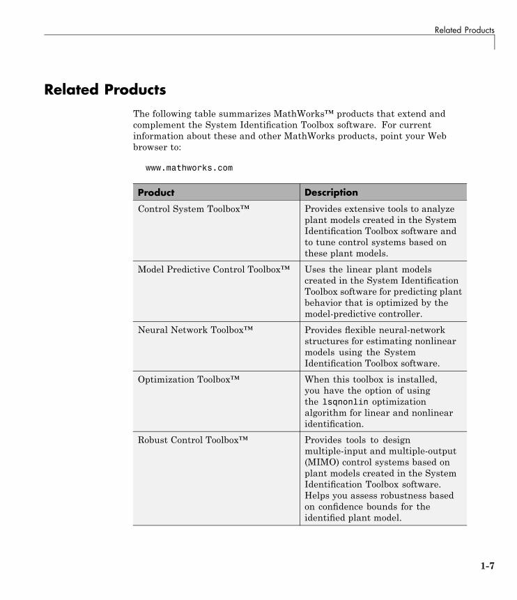
Related ProductsThe following table summarizes MathWorks™ products that extend andcomplement the System Identification Toolbox software. For currentinformation about these and other MathWorks products, point your Webbrowser to:
www.mathworks.com
Product Description
Control System Toolbox™ Provides extensive tools to analyzeplant models created in the SystemIdentification Toolbox software andto tune control systems based onthese plant models.
Model Predictive Control Toolbox™ Uses the linear plant modelscreated in the System IdentificationToolbox software for predicting plantbehavior that is optimized by themodel-predictive controller.
Neural Network Toolbox™ Provides flexible neural-networkstructures for estimating nonlinearmodels using the SystemIdentification Toolbox software.
Optimization Toolbox™ When this toolbox is installed,you have the option of usingthe lsqnonlin optimizationalgorithm for linear and nonlinearidentification.
Robust Control Toolbox™ Provides tools to designmultiple-input and multiple-output(MIMO) control systems based onplant models created in the SystemIdentification Toolbox software.Helps you assess robustness basedon confidence bounds for theidentified plant model.
1-7
1 Product Overview
Product Description
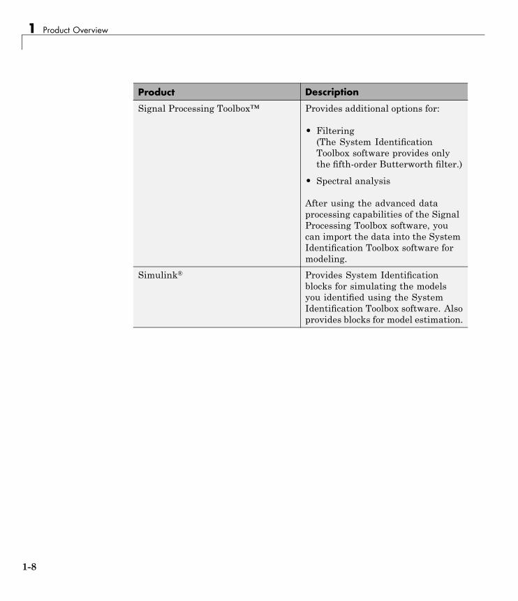
Signal Processing Toolbox™ Provides additional options for:
• Filtering(The System IdentificationToolbox software provides onlythe fifth-order Butterworth filter.)
• Spectral analysis
After using the advanced dataprocessing capabilities of the SignalProcessing Toolbox software, youcan import the data into the SystemIdentification Toolbox software formodeling.
Simulink® Provides System Identificationblocks for simulating the modelsyou identified using the SystemIdentification Toolbox software. Alsoprovides blocks for model estimation.
1-8
Learn More
Learn MoreThe goal of the System Identification Toolbox documentation is to provide youwith the necessary information to use this product. Additional resources areavailable to help you learn more about specific aspects of system identificationtheory and applications.
The following book describes methods for system identification and physicalmodeling:
Ljung, L., and T. Glad. Modeling of Dynamic Systems. PTR Prentice Hall,Upper Saddle River, NJ, 1994.
These books provide detailed information about system identification theoryand algorithms:
• Ljung, L. System Identification: Theory for the User. Second edition. PTRPrentice Hall, Upper Saddle River, NJ, 1999.
• Söderström, T., and P. Stoica. System Identification. Prentice HallInternational, London, 1989.
For information about working with frequency-domain data, see the followingbook:
Pintelon, R., and J. Schoukens. System Identification. A Frequency DomainApproach.Wiley-IEEE Press, New York, 2001.
For more information about systems and signals, see the following book:
Oppenheim, J., and Willsky, A.S. Signals and Systems. PTR Prentice Hall,Upper Saddle River, NJ, 1985.
The following textbook describes numerical techniques for parameterestimation using criterion minimization:
Dennis, J.E., Jr., and R.B. Schnabel. Numerical Methods for UnconstrainedOptimization and Nonlinear Equations. PTR Prentice Hall, Upper SaddleRiver, NJ, 1983.
1-9

1 Product Overview
1-10

2
Using This Product
• “When to Use the GUI Versus the Command Line” on page 2-2
• “Starting This Toolbox” on page 2-3
• “Steps for Using This Toolbox” on page 2-4
• “Tutorials to Help You Get Started” on page 2-6
2 Using This Product
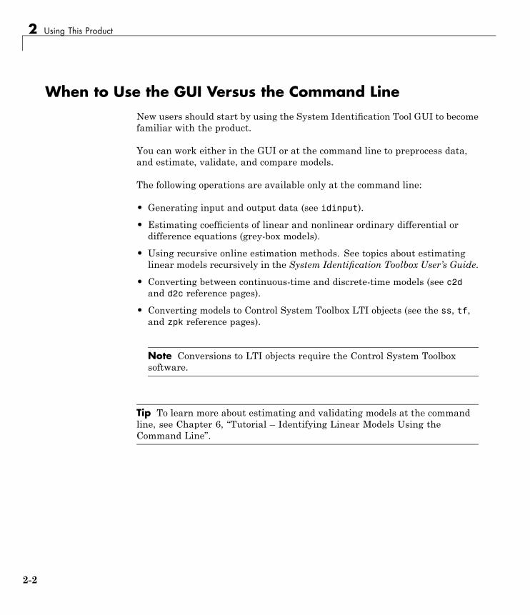
When to Use the GUI Versus the Command LineNew users should start by using the System Identification Tool GUI to becomefamiliar with the product.
You can work either in the GUI or at the command line to preprocess data,and estimate, validate, and compare models.
The following operations are available only at the command line:
• Generating input and output data (see idinput).
• Estimating coefficients of linear and nonlinear ordinary differential ordifference equations (grey-box models).
• Using recursive online estimation methods. See topics about estimatinglinear models recursively in the System Identification Toolbox User’s Guide.
• Converting between continuous-time and discrete-time models (see c2dand d2c reference pages).
• Converting models to Control System Toolbox LTI objects (see the ss, tf,and zpk reference pages).
Note Conversions to LTI objects require the Control System Toolboxsoftware.
Tip To learn more about estimating and validating models at the commandline, see Chapter 6, “Tutorial – Identifying Linear Models Using theCommand Line”.
2-2
Starting This Toolbox
Starting This ToolboxAfter installing the System Identification Toolbox product, you can start theSystem Identification Tool GUI or work at the command line.
For information about whether to use the GUI or the command line, see“When to Use the GUI Versus the Command Line” on page 2-2.
To open the System Identification Tool GUI:
• Select Start > Toolboxes > System Identification > SystemIdentification Tool from the MATLAB desktop.
Alternatively, you can open the System Identification Tool GUI by typing thefollowing command in the MATLAB Command Window:
ident
To work at the command line, type the commands directly in the MATLABCommand Window. For more information about supported commands, seethe reference pages.
2-3
2 Using This Product
Steps for Using This ToolboxSystem identification is an iterative process, where you identify models withdifferent structures from data and compare model performance. Ultimately,you choose the simplest model that best describes the dynamics of yoursystem.
Because this toolbox lets you estimate different model structures quickly, youshould try as many different structures as possible to see which one producesthe best results.
A system identification workflow might include the following tasks:
1 Process data for system identification by:
• Importing data into the MATLAB workspace.
• Representing data in the System Identification Tool GUI or as an iddataor idfrd object in the MATLAB workspace.
• Plotting data to examine both time- and frequency-domain behavior.
To analyze the data for the presence of constant offsets and trends,delay, feedback, and signal excitation levels, you can also use the advicecommand.
• Preprocessing data by removing offsets and linear trends, interpolatingmissing values, filtering to emphasize a specific frequency range, orresampling (interpolating or decimating) using a different time interval.
2 Identify linear or nonlinear models:
• Frequency-response models
• Impulse-response models
• Low-order transfer functions (process models)
• Input-output polynomial models
• State-space models
• Nonlinear black-box models
• Ordinary difference or differential equations (grey-box models)
2-4

Steps for Using This Toolbox
3 Validate models.
When you do not achieve a satisfactory model, try a different modelstructure and order or try another identification algorithm. In some cases,you can improve results by including a noise model.
You might need to preprocess your data before doing further estimation.For example, if there is too much high-frequency noise in your data, youmight need to filter or decimate (resample) the data before modeling.
4 Simulate or predict model output.
5 Design a controller for the estimated plant using other MathWorksproducts.
You can import an estimated linear model into the Control System Toolbox,Model Predictive Control Toolbox, Robust Control Toolbox, or Simulinkproducts for control design. For more information about linearizing anonlinear plant, see the linapp and linearize reference pages.
2-5
2 Using This Product
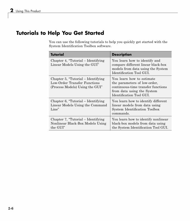
Tutorials to Help You Get StartedYou can use the following tutorials to help you quickly get started with theSystem Identification Toolbox software.
Tutorial Description
Chapter 4, “Tutorial – IdentifyingLinear Models Using the GUI”
You learn how to identify andcompare different linear black-boxmodels from data using the SystemIdentification Tool GUI.
Chapter 5, “Tutorial – IdentifyingLow-Order Transfer Functions(Process Models) Using the GUI”
You learn how to estimatethe parameters of low-order,continuous-time transfer functionsfrom data using the SystemIdentification Tool GUI.
Chapter 6, “Tutorial – IdentifyingLinear Models Using the CommandLine”
You learn how to identify differentlinear models from data usingSystem Identification Toolboxcommands.
Chapter 7, “Tutorial – IdentifyingNonlinear Black-Box Models Usingthe GUI”
You learn how to identify nonlinearblack-box models from data usingthe System Identification Tool GUI.
2-6

3
Choosing Which Models toEstimate
• “Data-Driven Modeling Using System Identification Toolbox Software”on page 3-2
• “When to Identify Linear Versus Nonlinear Models” on page 3-4
• “When to Identify Models from First Principles” on page 3-6
• “When to Identify Black-Box Models” on page 3-7
3 Choosing Which Models to Estimate
Data-Driven Modeling Using System Identification ToolboxSoftware
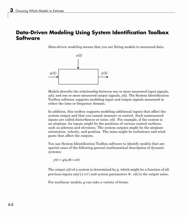
Data-driven modeling means that you are fitting models to measured data.
���� ����
����
Models describe the relationship between one or more measured input signals,u(t), and one or more measured output signals, y(t). The System IdentificationToolbox software supports modeling input and output signals measured ineither the time or frequency domain.
In addition, this toolbox supports modeling additional inputs that affect thesystem output and that you cannot measure or control. Such unmeasuredinputs are called disturbances or noise, e(t). For example, if the system isan airplane, its inputs might be the positions of various control surfaces,such as ailerons and elevators. The system outputs might be the airplaneorientation, velocity, and position. The noise might be turbulence and windgusts that affect the outputs.
You use System Identification Toolbox software to identify models that arespecial cases of the following general mathematical description of dynamicsystems:
y t g u v t( ) ( , ) ( )= +θ
The output y(t) of a system is determined by g, which might be a function of allprevious inputs u(s) ( s t≤ ) and system parameters θ . v(t) is the output noise.
For nonlinear models, g can take a variety of forms.
3-2
Data-Driven Modeling Using System Identification Toolbox™ Software
For linear models, the general symbolic model description is given by:
y Gu He= +
G is an operator that describes the system dynamics from the input to theoutput. G is often called a transfer function between u and y. H is an operatorthat describes the properties of the additive output disturbance and is called adisturbance model, or noise model. The actual disturbance contribution to theoutput, He, has real significance and contains all the known and unknowninfluences on the measured y not included in the input u. Therefore, if yourepeat and experiment with the same input, He explains why the outputsignal is different.
The source of the noise, e, need not have a physical significance. In the caseof an airplane, it is sufficient to estimate the noise in a black-box manner asarising from a white noise source via a transfer function H. Thus, you do notneed to know how the wind gusts and turbulence are generated physicallyand all that matters are the characteristics of He, such as the frequencycontent of the spectrum of He.
If you know that your measured data includes noise, you can choose a modelstructure that computes H to produce a more accurate dynamic model. Formore information about choosing to model noise in linear black-box models,see “When to Identify Black-Box Models” on page 3-7.
3-3

3 Choosing Which Models to Estimate
When to Identify Linear Versus Nonlinear ModelsYou can identify both linear and nonlinear models using System IdentificationToolbox software. In practice, all systems are nonlinear and the output is anonlinear function of the input variables. However, a linear model is oftensufficient to accurately describe the system dynamics.
Follow these guidelines to choose between using nonlinear and linearblack-box models:
• When you have physical insight that the system is nonlinear, trytransforming your input and output variables such that the relationshipbetween the transformed variables is linear.
For example, you might be dealing with a system that has current andvoltage as inputs to an immersion heater, and the temperature of theheated liquid as an output. In this case, the output depends on the inputsvia the power of the heater, which is equal to the product of current andvoltage. Instead of fitting a nonlinear model to two-input and one-outputdata, you can create a new input variable by taking the product of currentand voltage and then fitting a linear model to the single-input/single-outputdata.
• Plot the response of the system to a specific input. If you notice that theresponses are different depending on the input level or input sign, use anonlinear model. For example, you might see that the output response toan input step up is much faster than the response to a step down.
• Try identifying several linear models of varying complexity. If the modeloutput does not adequately reproduce the measured output, you mightneed to use a nonlinear model. Noisy data might also cause a model tofail reproducing measured output.
For a grey-box model, its linear or nonlinear structure is set by its ordinarydifferential or difference equations (ODEs). For more information aboutchoosing this type of model, see “When to Identify Models from FirstPrinciples” on page 3-6.
For a black-box model, you can choose whether to estimate linear or nonlinearmodels. Linear approximations are very useful because they are simple andprovide good results in many situations. Therefore, always estimate linear
3-4

When to Identify Linear Versus Nonlinear Models
models first and see how well these models represent the dynamics. Formore information about choosing this type of model, see “When to IdentifyBlack-Box Models” on page 3-7.
Note You can only use this toolbox to estimate discrete-time nonlinearblack-box models from time-domain data.
3-5
3 Choosing Which Models to Estimate
When to Identify Models from First PrinciplesA grey-box model has a known mathematical structure and unknownparameters. Use this approach if you understand the physics of your systemand can represent the system dynamics using ordinary differential ordifference equations (ODEs).
You capture the ODE and the parameters you want to estimate in an M-fileor MEX-file, and use the System Identification Toolbox product to estimatethe model parameters. For example, to estimate the parameters of a transferfunction that you defined, you must first represent the transfer function instate-space form.
Grey-box modeling has the following advantages over black-box modeling:
• You can impose known constraints on model characteristics, such as modelparameters and noise variance.
• There are potentially fewer parameters to estimate.
• You can specify couplings between parameters when defining the modelstructure.
• In the nonlinear case, you can specify the dynamic equations explicitly.
Grey-box modeling is preferred. However, grey-box modeling requires thatyou know the relationship between the system variables and the parameters,which can be time consuming. For an alternative to grey-box modeling, see“When to Identify Black-Box Models” on page 3-7.
For information about estimating linear and nonlinear grey-box models, seethe System Identification Toolbox User’s Guide.
3-6

When to Identify Black-Box Models
When to Identify Black-Box ModelsSystem identification is especially useful for modeling systems that youcannot easily represent in terms of first principles or known physical laws.The parameters of a black-box model might not have a physical interpretation.
Black-box models can be linear or nonlinear. Linear black-box models canalso be continuous-time or discrete-time models.
Black-box modeling has the following advantages:
• You do not need to know the structure of your model to get started quickly.
• You can estimate many model structures and compare them to choose thebest one.
System Identification Toolbox software provides linear black-box modelstructures that let you model noise explicitly. For example, you can modelnoise for a low-order transfer function or a state-space model. Someinput-output polynomial models, such as the ARMAX or Box-Jenkins (BJ)structure, provide additional parameters to model noise and decouple thedynamics from the noise.
Note Nonlinear black-box models do not support parametric noise modeling.
You might choose a linear model structure with a noise model in the followingsituations:
• You are specifically interested in a noise model, such as when developingnoise-cancelation and noise-attenuation technologies, or for disturbancerejection in control design applications.
• You want to use the noise characteristics to improve the estimation of thedynamic model by emphasizing the frequencies that are least affected bynoise during the estimation.
3-7

3 Choosing Which Models to Estimate
3-8
4
Tutorial – IdentifyingLinear Models Using theGUI
• “About This Tutorial” on page 4-2
• “Preparing Data for System Identification” on page 4-4
• “Saving the GUI Session” on page 4-20
• “Estimating Linear Models Using Quick Start” on page 4-23
• “Estimating Accurate Linear Models” on page 4-30
• “Viewing Model Parameters” on page 4-43
• “Exporting the Model to the MATLAB Workspace” on page 4-47
• “Exporting the Model to the LTI Viewer” on page 4-49
4 Tutorial – Identifying Linear Models Using the GUI
About This Tutorial
In this section...
“Objectives” on page 4-2“Data Description” on page 4-2
ObjectivesEstimate and validate linear models from single-input/single-output (SISO)data to find the one that best describes the system dynamics.
After completing this tutorial, you will be able to accomplish the followingtasks using the System Identification Tool GUI:
• Import data arrays from the MATLAB workspace into the GUI.
• Plot the data.
• Process data by removing offsets from the input and output signals.
• Estimate, validate, and compare linear models.
• Export models to the MATLAB workspace.
Note The tutorial uses time-domain data to demonstrate how youcan estimate linear models. The same workflow applies to fittingfrequency-domain data.
This tutorial is based on the example in section 17.3 of System Identification:Theory for the User, Second Edition, by Lennart Ljung, Prentice Hall PTR,1999.
Data DescriptionThis tutorial uses the data file dryer2.mat, which containssingle-input/single-output (SISO) time-domain data from Feedback ProcessTrainer PT326. The input and output signals each contain 1000 data samples.
4-2

About This Tutorial
This system heats the air at the inlet using a mesh of resistor wire, similar toa hair dryer. The input is the power supplied to the resistor wires, and theoutput is the air temperature at the outlet.
4-3
4 Tutorial – Identifying Linear Models Using the GUI
Preparing Data for System Identification
In this section...
“Loading Data into the MATLAB Workspace” on page 4-4“Opening the System Identification Tool GUI” on page 4-4“Importing Data Arrays into the System Identification Tool” on page 4-5“Plotting and Processing Data” on page 4-10
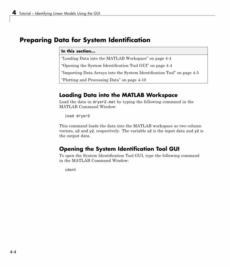
Loading Data into the MATLAB WorkspaceLoad the data in dryer2.mat by typing the following command in theMATLAB Command Window:
load dryer2
This command loads the data into the MATLAB workspace as two columnvectors, u2 and y2, respectively. The variable u2 is the input data and y2 isthe output data.
Opening the System Identification Tool GUITo open the System Identification Tool GUI, type the following commandin the MATLAB Command Window:
ident
4-4
Preparing Data for System Identification
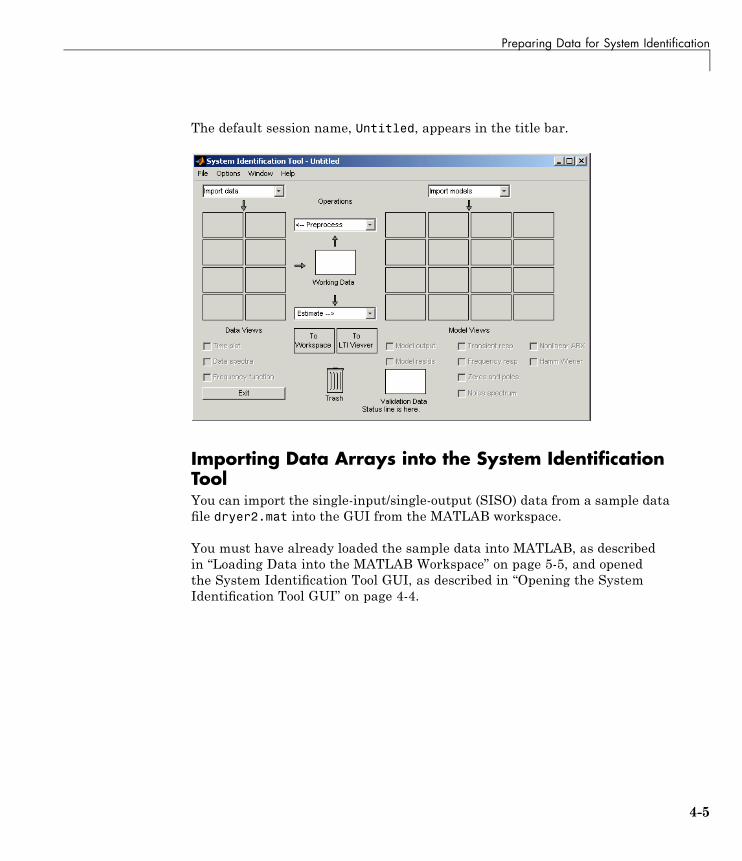
The default session name, Untitled, appears in the title bar.
Importing Data Arrays into the System IdentificationToolYou can import the single-input/single-output (SISO) data from a sample datafile dryer2.mat into the GUI from the MATLAB workspace.
You must have already loaded the sample data into MATLAB, as describedin “Loading Data into the MATLAB Workspace” on page 5-5, and openedthe System Identification Tool GUI, as described in “Opening the SystemIdentification Tool GUI” on page 4-4.
4-5
4 Tutorial – Identifying Linear Models Using the GUI
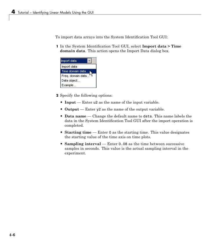
To import data arrays into the System Identification Tool GUI:
1 In the System Identification Tool GUI, select Import data > Timedomain data. This action opens the Import Data dialog box.
2 Specify the following options:
• Input — Enter u2 as the name of the input variable.
• Output — Enter y2 as the name of the output variable.
• Data name— Change the default name to data. This name labels thedata in the System Identification Tool GUI after the import operation iscompleted.
• Starting time — Enter 0 as the starting time. This value designatesthe starting value of the time axis on time plots.
• Sampling interval — Enter 0.08 as the time between successivesamples in seconds. This value is the actual sampling interval in theexperiment.
4-6
Preparing Data for System Identification
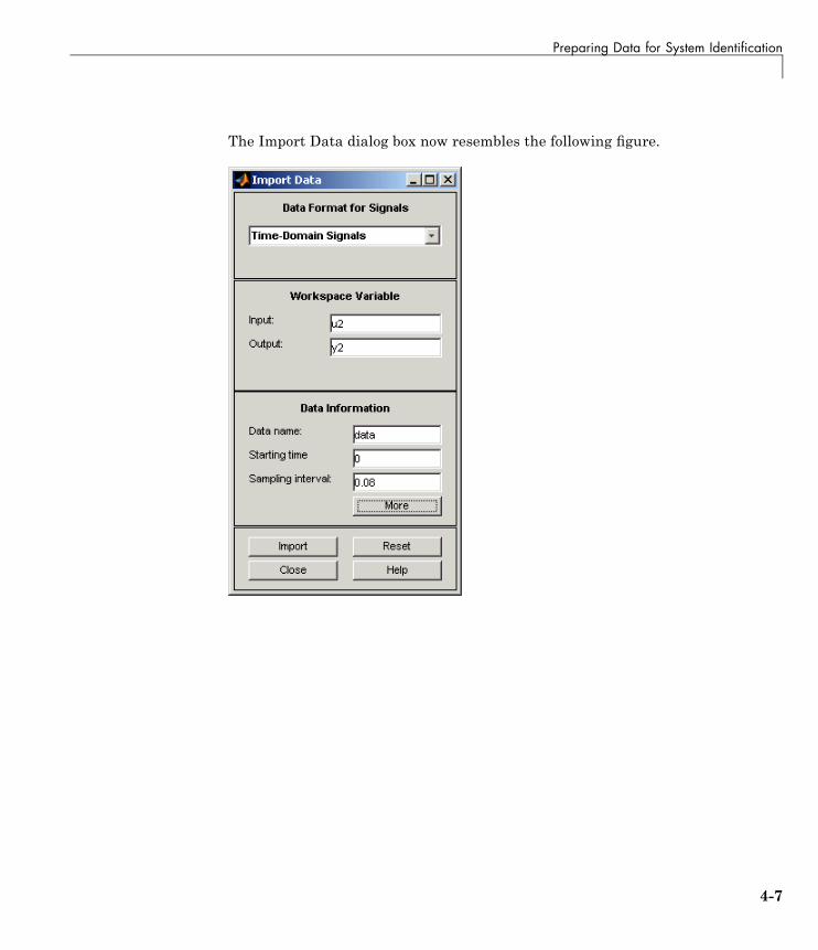
The Import Data dialog box now resembles the following figure.
4-7
4 Tutorial – Identifying Linear Models Using the GUI
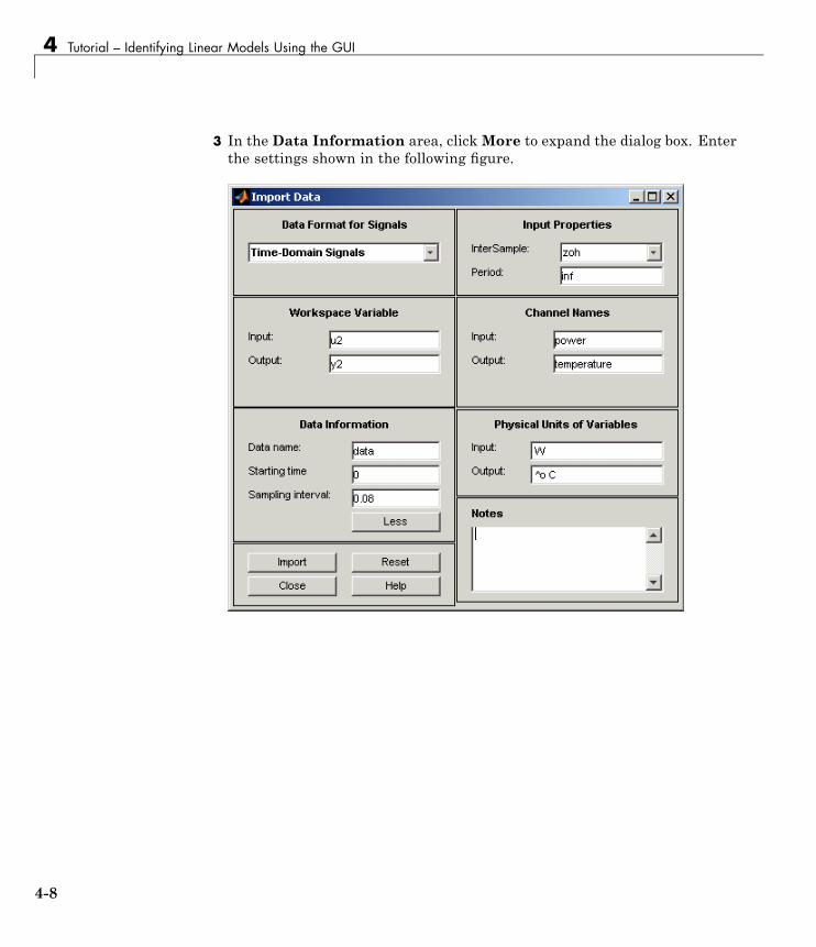
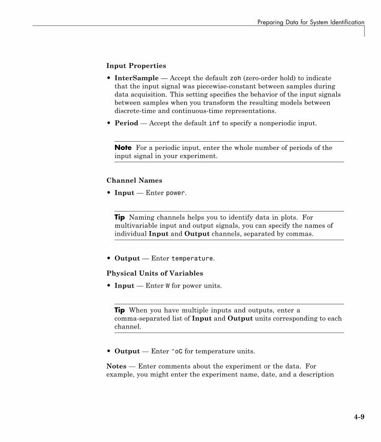
3 In the Data Information area, clickMore to expand the dialog box. Enterthe settings shown in the following figure.
4-8
Preparing Data for System Identification
Input Properties
• InterSample — Accept the default zoh (zero-order hold) to indicatethat the input signal was piecewise-constant between samples duringdata acquisition. This setting specifies the behavior of the input signalsbetween samples when you transform the resulting models betweendiscrete-time and continuous-time representations.
• Period— Accept the default inf to specify a nonperiodic input.
Note For a periodic input, enter the whole number of periods of theinput signal in your experiment.
Channel Names
• Input — Enter power.
Tip Naming channels helps you to identify data in plots. Formultivariable input and output signals, you can specify the names ofindividual Input and Output channels, separated by commas.
• Output — Enter temperature.
Physical Units of Variables
• Input — Enter W for power units.
Tip When you have multiple inputs and outputs, enter acomma-separated list of Input and Output units corresponding to eachchannel.
• Output — Enter ^oC for temperature units.
Notes — Enter comments about the experiment or the data. Forexample, you might enter the experiment name, date, and a description
4-9
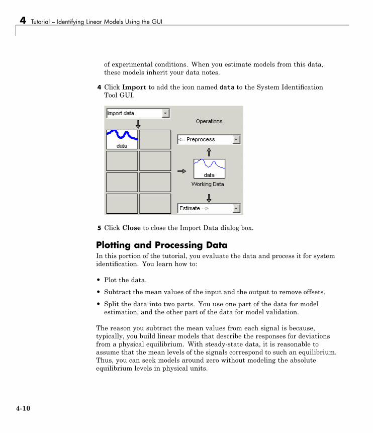
4 Tutorial – Identifying Linear Models Using the GUI
of experimental conditions. When you estimate models from this data,these models inherit your data notes.
4 Click Import to add the icon named data to the System IdentificationTool GUI.
5 Click Close to close the Import Data dialog box.
Plotting and Processing DataIn this portion of the tutorial, you evaluate the data and process it for systemidentification. You learn how to:
• Plot the data.
• Subtract the mean values of the input and the output to remove offsets.
• Split the data into two parts. You use one part of the data for modelestimation, and the other part of the data for model validation.
The reason you subtract the mean values from each signal is because,typically, you build linear models that describe the responses for deviationsfrom a physical equilibrium. With steady-state data, it is reasonable toassume that the mean levels of the signals correspond to such an equilibrium.Thus, you can seek models around zero without modeling the absoluteequilibrium levels in physical units.
4-10
Preparing Data for System Identification
You must have already imported data into the System Identification Tool, asdescribed in “Importing Data Arrays into the System Identification Tool”on page 4-5.
To plot and process the data:
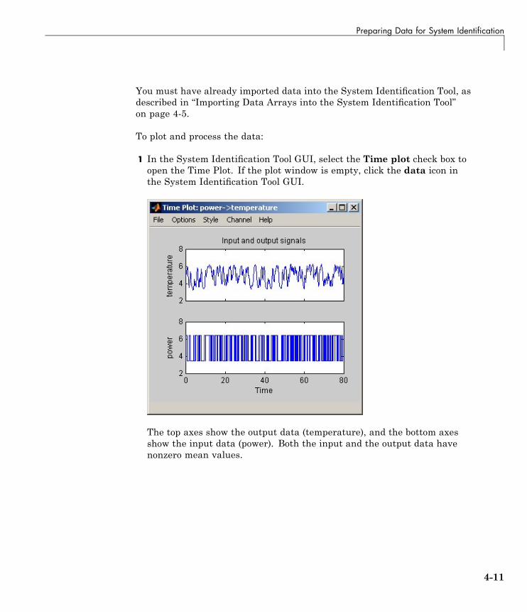
1 In the System Identification Tool GUI, select the Time plot check box toopen the Time Plot. If the plot window is empty, click the data icon inthe System Identification Tool GUI.
The top axes show the output data (temperature), and the bottom axesshow the input data (power). Both the input and the output data havenonzero mean values.
4-11
4 Tutorial – Identifying Linear Models Using the GUI
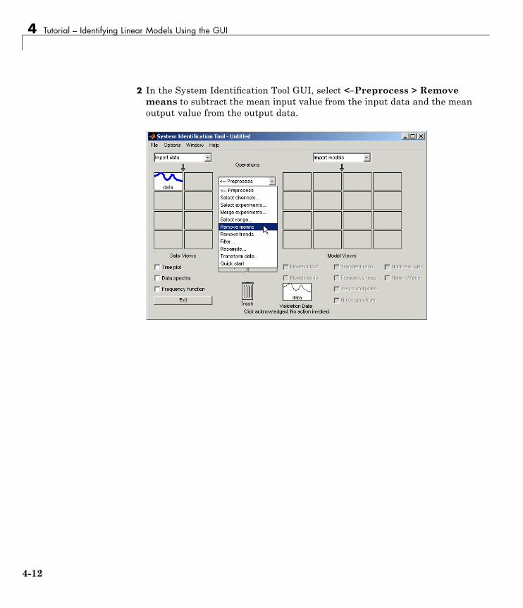
2 In the System Identification Tool GUI, select <–Preprocess > Removemeans to subtract the mean input value from the input data and the meanoutput value from the output data.
4-12
Preparing Data for System Identification
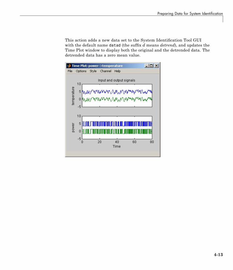
This action adds a new data set to the System Identification Tool GUIwith the default name datad (the suffix d means detrend), and updates theTime Plot window to display both the original and the detrended data. Thedetrended data has a zero mean value.
4-13
4 Tutorial – Identifying Linear Models Using the GUI
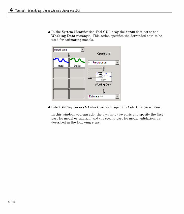
3 In the System Identification Tool GUI, drag the datad data set to theWorking Data rectangle. This action specifies the detrended data to beused for estimating models.
4 Select <–Preprocess > Select range to open the Select Range window.
In this window, you can split the data into two parts and specify the firstpart for model estimation, and the second part for model validation, asdescribed in the following steps.
4-14
Preparing Data for System Identification
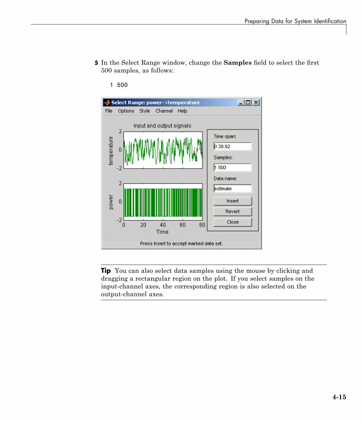
5 In the Select Range window, change the Samples field to select the first500 samples, as follows:
1 500
Tip You can also select data samples using the mouse by clicking anddragging a rectangular region on the plot. If you select samples on theinput-channel axes, the corresponding region is also selected on theoutput-channel axes.
4-15
4 Tutorial – Identifying Linear Models Using the GUI
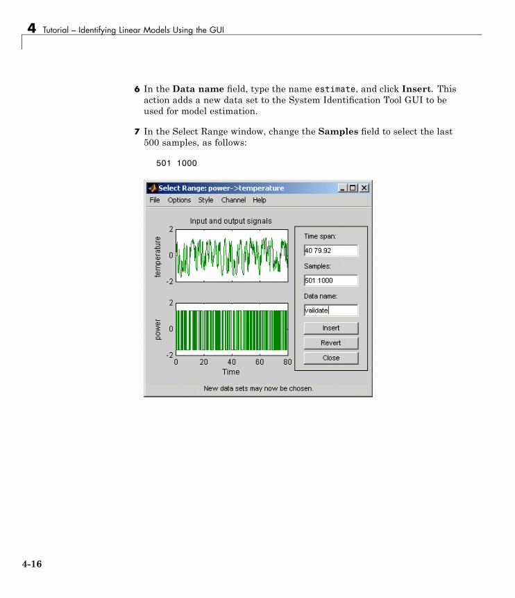
6 In the Data name field, type the name estimate, and click Insert. Thisaction adds a new data set to the System Identification Tool GUI to beused for model estimation.
7 In the Select Range window, change the Samples field to select the last500 samples, as follows:
501 1000
4-16
Preparing Data for System Identification
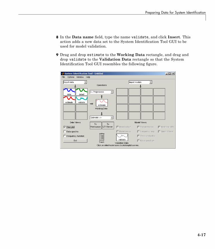
8 In the Data name field, type the name validate, and click Insert. Thisaction adds a new data set to the System Identification Tool GUI to beused for model validation.
9 Drag and drop estimate to the Working Data rectangle, and drag anddrop validate to the Validation Data rectangle so that the SystemIdentification Tool GUI resembles the following figure.
4-17
4 Tutorial – Identifying Linear Models Using the GUI
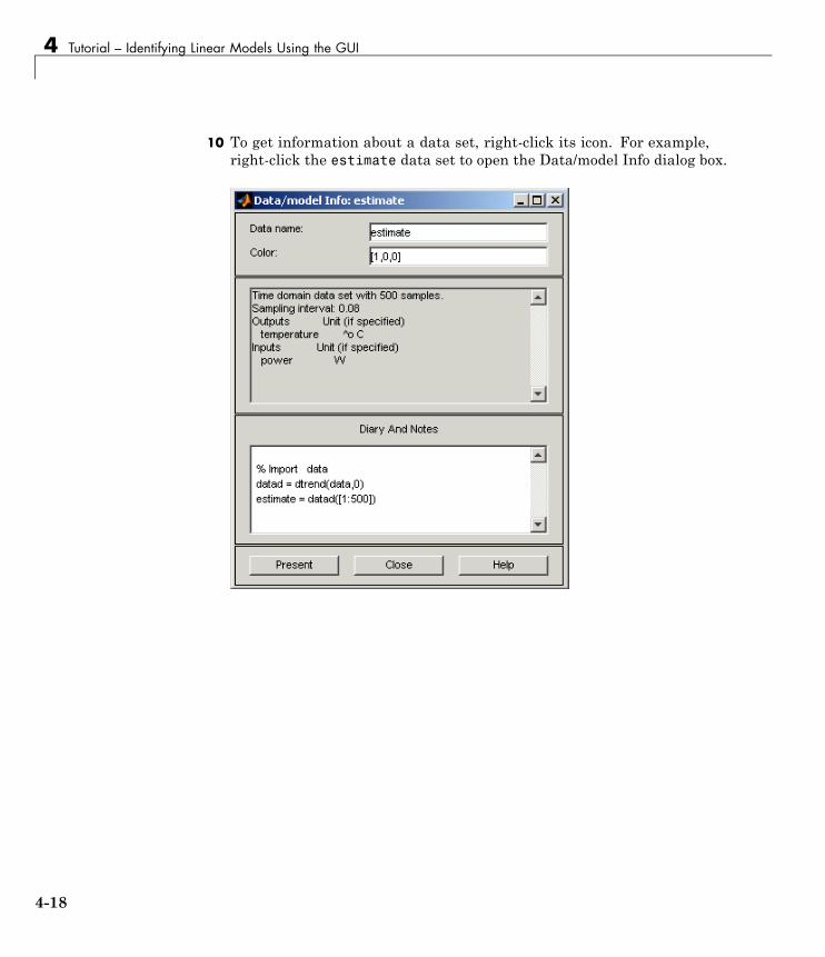
10 To get information about a data set, right-click its icon. For example,right-click the estimate data set to open the Data/model Info dialog box.
4-18
Preparing Data for System Identification
In the Data/model Info dialog box, you can perform the following actions:
• Change the name of the data set in the Data name field.
• Change the color of the data icon by changing the RGB values (relativeamounts of red, green, and blue). Each value is between 0 and 1. Forexample, [1,0,0] indicates that only red is present, and no green andblue are mixed into the overall color.
• In the noneditable area, view the total number of samples, the samplinginterval, and the output and input channel names and units.
• In the editable Diary And Notes area, view or edit the actions youperformed on this data set. The actions are translated into commandsequivalent to your GUI operations. For example, the estimate dataset is a result of importing the data, detrending the mean values, andselecting the first 500 samples of the data:
load dryer2% Import datadatad = detrend(data,0)estimate = datad([1:500])
For more information about these and other toolbox commands, see thereference page corresponding to each command.
Tip As an alternative shortcut, you can select Preprocess > Quick startfrom the System Identification Tool GUI to perform all of the data processingsteps in this tutorial.
Learn MoreFor information about supported data processing operations, such asresampling and filtering the data, see the System Identification ToolboxUser’s Guide.
4-19
4 Tutorial – Identifying Linear Models Using the GUI
Saving the GUI SessionAfter you process the data, as described in “Plotting and Processing Data”on page 4-10, you can delete any data sets in the window that you do notneed for estimation and validation, and save your session. You can open thissession later and use it as a starting point for model estimation and validationwithout repeating these preparatory steps.
You must have already processed the data into the System Identification Tool,as described in “Plotting and Processing Data” on page 4-10.
To delete specific data sets from a session and save the session:
1 In the System Identification Tool GUI, drag and drop the data data setinto the Trash.
2 Drag and drop the datad data set into the Trash.
Note Moving items to the Trash does not delete them. To permanentlydelete items, select Options > Empty trash in the System IdentificationTool GUI.
4-20
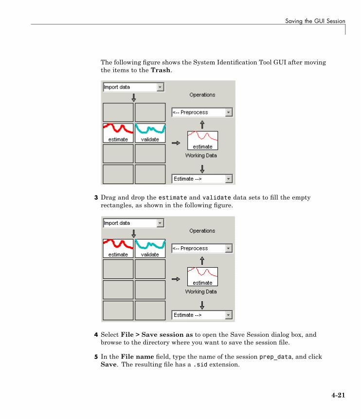
Saving the GUI Session
The following figure shows the System Identification Tool GUI after movingthe items to the Trash.
3 Drag and drop the estimate and validate data sets to fill the emptyrectangles, as shown in the following figure.
4 Select File > Save session as to open the Save Session dialog box, andbrowse to the directory where you want to save the session file.
5 In the File name field, type the name of the session prep_data, and clickSave. The resulting file has a .sid extension.
4-21
4 Tutorial – Identifying Linear Models Using the GUI
Tip You can open a saved session when starting the System IdentificationTool. For example, you can type the following command in the MATLABCommand Window:
ident('prep_data')
For more information about managing sessions, see the topics on workingwith the System Identification Tool GUI in the System Identification ToolboxUser’s Guide.
4-22
Estimating Linear Models Using Quick Start
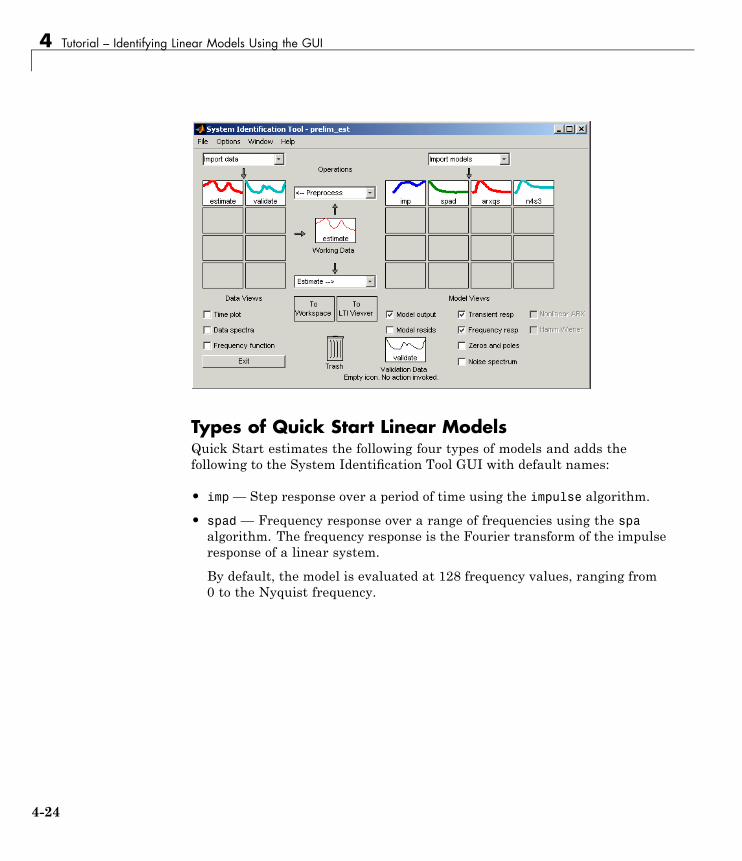
Estimating Linear Models Using Quick Start
In this section...
“How to Estimate Linear Models Using Quick Start” on page 4-23“Types of Quick Start Linear Models” on page 4-24“Validating the Quick Start Models” on page 4-25
How to Estimate Linear Models Using Quick StartYou can use the Quick Start feature in the System Identification Toolboxestimate linear models. Quick Start might produce the final linear modelsyou decide to use, or provide you with information required to configure theestimation of accurate parametric models, such as time constants, inputdelays, and resonant frequencies.
You must have already processed the data for estimation, as described in“Plotting and Processing Data” on page 4-10.
To identify linear models:
• In the System Identification Tool GUI, select Estimate > Quick start.
This action generates plots of step response, frequency-response, and theoutput of state-space and polynomial models. For more information aboutthese plots, see “Validating the Quick Start Models” on page 4-25.
4-23
4 Tutorial – Identifying Linear Models Using the GUI
Types of Quick Start Linear ModelsQuick Start estimates the following four types of models and adds thefollowing to the System Identification Tool GUI with default names:
• imp— Step response over a period of time using the impulse algorithm.
• spad — Frequency response over a range of frequencies using the spaalgorithm. The frequency response is the Fourier transform of the impulseresponse of a linear system.
By default, the model is evaluated at 128 frequency values, ranging from0 to the Nyquist frequency.
4-24
Estimating Linear Models Using Quick Start
• arxqs—Fourth-order autoregressive (ARX) model using the arx algorithm.
This model is parametric and has the following structure:
y t a y t a y t n
u t n b u t nna a
k nb k
( ) ( ) ( )( ) (
+ − + + − =− + + − −
1 1 …… b1 nn e tb + +1) ( )
y(t) represents the output at time t, u(t) represents the input at time t,na is the number of poles, nb is the number of b parameters (equal to thenumber of zeros plus 1), nk is the number of samples before the input affectsoutput of the system (called the delay or dead time of the model), and e(t) isthe white-noise disturbance. The System Identification Toolbox productestimates the parameters a an1 … and b bn1 … using the input and outputdata from the estimation data set.
In arxqs, na=nb=4, and nk is estimated from the step response model imp.
• n4s3 — State-space model calculated using n4sid. The algorithmautomatically selects the model order (in this case, 3).
This model is parametric and has the following structure:
x t Ax t Bu t Ke ty t Cx t Du t e t( ) ( ) ( ) ( )( ) ( ) ( ) ( )
+ = + += + +1
y(t) represents the output at time t, u(t) represents the input at time t, xis the state vector, and e(t) is the white-noise disturbance. The SystemIdentification Toolbox product estimates the state-space matrices A, B,C, D, and K.
Validating the Quick Start ModelsQuick Start generates the following plots during model estimation to help youvalidate the quality of the models:
• Step-response plot
• Frequency-response plot
• Model-output plot
4-25
4 Tutorial – Identifying Linear Models Using the GUI
You must have already estimated models using Quick Start to generatethese plots, as described in “How to Estimate Linear Models Using QuickStart” on page 4-23.
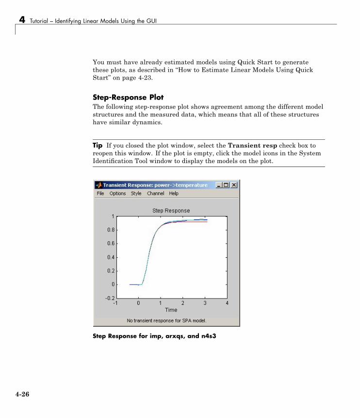
Step-Response PlotThe following step-response plot shows agreement among the different modelstructures and the measured data, which means that all of these structureshave similar dynamics.
Tip If you closed the plot window, select the Transient resp check box toreopen this window. If the plot is empty, click the model icons in the SystemIdentification Tool window to display the models on the plot.
Step Response for imp, arxqs, and n4s3
4-26
Estimating Linear Models Using Quick Start
Tip You can use the step-response plot to estimate the dead time of linearsystems. For example, the previous step-response plot shows a time delay ofabout 0.25 s before the system responds to the input. This response delay,or dead time, is approximately equal to about three samples because thesampling interval is 0.08 s for this data set.
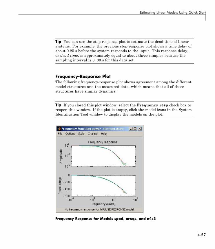
Frequency-Response PlotThe following frequency-response plot shows agreement among the differentmodel structures and the measured data, which means that all of thesestructures have similar dynamics.
Tip If you closed this plot window, select the Frequency resp check box toreopen this window. If the plot is empty, click the model icons in the SystemIdentification Tool window to display the models on the plot.
Frequency Response for Models spad, arxqs, and n4s3
4-27
4 Tutorial – Identifying Linear Models Using the GUI
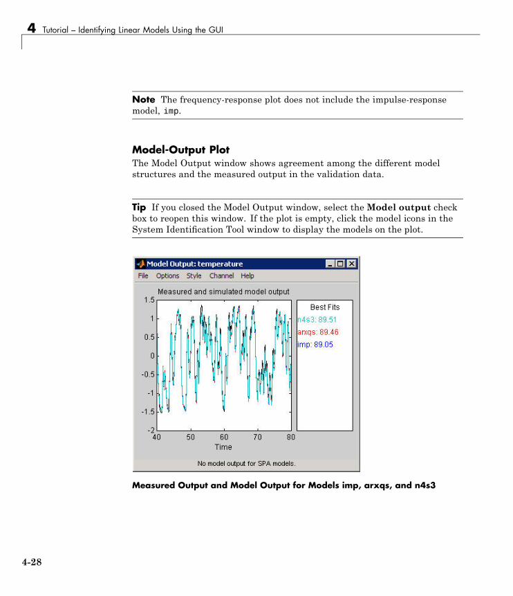
Note The frequency-response plot does not include the impulse-responsemodel, imp.
Model-Output PlotThe Model Output window shows agreement among the different modelstructures and the measured output in the validation data.
Tip If you closed the Model Output window, select theModel output checkbox to reopen this window. If the plot is empty, click the model icons in theSystem Identification Tool window to display the models on the plot.
Measured Output and Model Output for Models imp, arxqs, and n4s3
4-28
Estimating Linear Models Using Quick Start
The model-output plot shows the model response to the input in the validationdata. The fit values for each model are summarized in the Best Fits areaof the Model Output window. The models in the Best Fits list are orderedfrom best at the top to worst at the bottom. The fit between the two curves iscomputed such that 100 means a perfect fit, and 0 indicates a poor fit (thatis, the model output has the same fit to the measured output as the mean ofthe measured output).
In this example, the output of the models matches the validation data output,which indicates that the models seem to capture the main system dynamicsand that linear modeling is sufficient.
Tip To compare predicted model output instead of simulated output, selectthis option from the Options menu in the Model Output window.
4-29
4 Tutorial – Identifying Linear Models Using the GUI
Estimating Accurate Linear Models
In this section...
“Strategy for Estimating Accurate Models” on page 4-30“Estimating Possible Model Orders” on page 4-30“Identifying State-Space Models” on page 4-35“Identifying ARMAX Input-Output Polynomial Models” on page 4-36“Choosing the Best Model” on page 4-39
Strategy for Estimating Accurate ModelsThe linear models you estimated in “Estimating Linear Models Using QuickStart” on page 4-23 showed that a linear model sufficiently represents thedynamics of the system.
In this portion of the tutorial, you get accurate parametric models byperforming the following tasks:
1 Identifying initial model orders and delays from your data using a simple,polynomial model structure (ARX).
2 Exploring more complex model structures with orders and delays close tothe initial values you found.
The resulting models are discrete-time models.
Tip You can convert a linear discrete-time model to a continuous-timemodel using the d2c command. For more information, see the correspondingreference page.
Estimating Possible Model OrdersTo identify black-box models, you must specify the model order. However,how can you tell what model orders to specify for your black-box models? Toanswer this question, you can estimate simple polynomial (ARX) models for arange of orders and delays and compare the performance of these models. You
4-30
Estimating Accurate Linear Models
choose the orders and delays that correspond to the best model fit as an initialguess for more accurate modeling.
About ARX ModelsFor a single-input/single-output system (SISO), the ARX model structure is:
y t a y t a y t n
u t n b u t nna a
k nb k
( ) ( ) ( )( ) (
+ − + + − =− + + − −
1 1 …… b1 nn e tb + +1) ( )
y(t) represents the output at time t, u(t) represents the input at time t, na is thenumber of poles, nb is the number of zeros plus 1, nk is the input delay—thenumber of samples before the input affects the system output (called delay ordead time of the model), and e(t) is the white-noise disturbance.
You specify the model orders na, nb, and nk to estimate ARX models. TheSystem Identification Toolbox product estimates the parameters a an1 …
and b bn1 … from the data.
How to Estimate Model Orders
1 In the System Identification Tool GUI, select Estimate > Linearparametric models to open the Linear Parametric Models dialog box.
The ARX model is already selected in the Structure list.
4-31
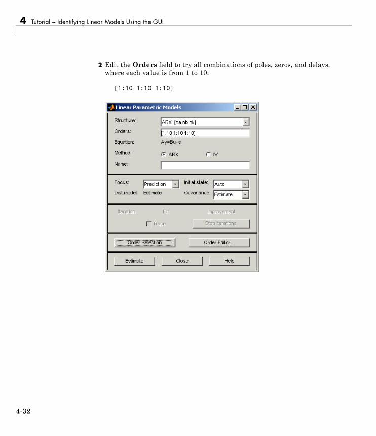
4 Tutorial – Identifying Linear Models Using the GUI
2 Edit the Orders field to try all combinations of poles, zeros, and delays,where each value is from 1 to 10:
[1:10 1:10 1:10]
4-32
Estimating Accurate Linear Models
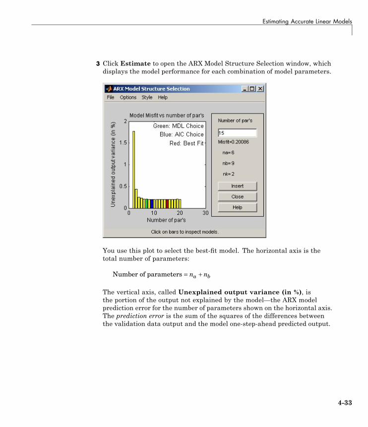
3 Click Estimate to open the ARX Model Structure Selection window, whichdisplays the model performance for each combination of model parameters.
You use this plot to select the best-fit model. The horizontal axis is thetotal number of parameters:
Number of parameters = +n na b
The vertical axis, called Unexplained output variance (in %), isthe portion of the output not explained by the model—the ARX modelprediction error for the number of parameters shown on the horizontal axis.The prediction error is the sum of the squares of the differences betweenthe validation data output and the model one-step-ahead predicted output.
4-33
4 Tutorial – Identifying Linear Models Using the GUI
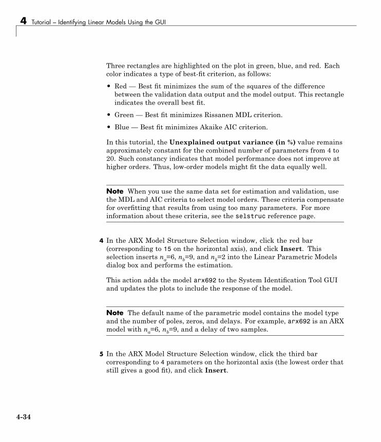
Three rectangles are highlighted on the plot in green, blue, and red. Eachcolor indicates a type of best-fit criterion, as follows:
• Red — Best fit minimizes the sum of the squares of the differencebetween the validation data output and the model output. This rectangleindicates the overall best fit.
• Green — Best fit minimizes Rissanen MDL criterion.
• Blue — Best fit minimizes Akaike AIC criterion.
In this tutorial, the Unexplained output variance (in %) value remainsapproximately constant for the combined number of parameters from 4 to20. Such constancy indicates that model performance does not improve athigher orders. Thus, low-order models might fit the data equally well.
Note When you use the same data set for estimation and validation, usethe MDL and AIC criteria to select model orders. These criteria compensatefor overfitting that results from using too many parameters. For moreinformation about these criteria, see the selstruc reference page.
4 In the ARX Model Structure Selection window, click the red bar(corresponding to 15 on the horizontal axis), and click Insert. Thisselection inserts na=6, nb=9, and nk=2 into the Linear Parametric Modelsdialog box and performs the estimation.
This action adds the model arx692 to the System Identification Tool GUIand updates the plots to include the response of the model.
Note The default name of the parametric model contains the model typeand the number of poles, zeros, and delays. For example, arx692 is an ARXmodel with na=6, nb=9, and a delay of two samples.
5 In the ARX Model Structure Selection window, click the third barcorresponding to 4 parameters on the horizontal axis (the lowest order thatstill gives a good fit), and click Insert.
4-34

Estimating Accurate Linear Models
• This selection inserts na=2, nb=2, and nk=3 (a delay of three samples) intothe Linear Parametric Models dialog box and performs the estimation.
• The model arx223 is added to the System Identification Tool GUI andthe plots are updated to include its response and output.
6 Click Close to close the ARX Model Structure Selection window.
Identifying State-Space ModelsBy estimating ARX models for different order combinations, as described in“Estimating Possible Model Orders” on page 4-30, you identified the numberof poles, zeros, and delays that provide a good starting point for systematicallyexploring different models.
The overall best fit for this system corresponds to a model with six poles, ninezeros, and a delay of two samples. It also showed that a low-order model withna=2 (two poles), nb=2 (one zero), and nk=3 (input-output delay) also providesa good fit. Thus, you should explore model orders close to these values.
In this portion of the tutorial, you estimate a state-space model.
About State-Space ModelsThe general state-space model structure (innovation form) is:
x t Ax t Bu t Ke ty t Cx t Du t e t( ) ( ) ( ) ( )( ) ( ) ( ) ( )
+ = + += + +1
y(t) represents the output at time t, u(t) represents the input at time t, x(t) isthe state vector at time t, and e(t) is the white-noise disturbance.
You must specify a single integer as the model order (dimension of the statevector) to estimate a state-space model. By default, the delay equals 1. TheSystem Identification Toolbox product estimates the state-space matrices A,B, C, D, and K from the data.
The state-space model structure is a good choice for quick estimation becauseit requires that you specify only two parameters to get started: n is thenumber of poles (the size of the A matrix) and nk is the delay.
4-35
4 Tutorial – Identifying Linear Models Using the GUI
How to Estimate State-Space Models
1 In the System Identification Tool GUI, select Estimate > Linearparametric models to open the Linear Parametric Models dialog box.
2 From the Structure list, select State Space: n [nk].
3 In the Orders field, type 6 to create a sixth-order state-space model.
This choice is based on the fact that the best-fit ARX model has six poles.
Tip Although this tutorial estimates a sixth-order state-space model, youmight want to explor whether a lower-order model adequately representsthe system dynamics.
4 Click Estimate to add a state-space model called n4s6 to the SystemIdentification Tool GUI.
Tip If you closed the Model Output window, you can regenerate it byselecting the Model output check box in the System Identification ToolGUI. If the new model does not appear on the plot, click the model icon inthe System Identification Tool GUI to make the model active.
Learn MoreTo learn more about identifying state-space models, see the correspondingtopic in the System Identification Toolbox User’s Guide.
Identifying ARMAX Input-Output Polynomial ModelsBy estimating ARX models for different order combinations, as described in“Estimating Possible Model Orders” on page 4-30, you identified the numberof poles, zeros, and delays that provide a good starting point for systematicallyexploring different models.
The overall best fit for this system corresponds to a model with six poles, ninezeros, and a delay of two samples. It also showed that a low-order model with
4-36
Estimating Accurate Linear Models
na=2 (two poles), nb=2 (one zero), and nk=3 also provides a good fit. Thus, youshould explore model orders close to these values.
In this portion of the tutorial, you estimate an ARMAX input-outputpolynomial model.
About ARMAX ModelsFor a single-input/single-output system (SISO), the ARMAX polynomialmodel structure is:
y t a y t a y t n
u t n b u t nna a
k nb k
( ) ( ) ( )( ) (
+ − + + − =− + + − −
1 1 …… b1 nn
e t c e t c e t nb
nc c
+ ++ − + + −
111
)( ) ( ) ( ) …
y(t) represents the output at time t, u(t) represents the input at time t, na isthe number of poles for the dynamic model, nb is the number of zeros plus 1, ncis the number of poles for the disturbance model, nk is the number of samplesbefore the input affects output of the system (called the delay or dead time ofthe model), and e(t) is the white-noise disturbance.
Note The ARMAX model is more flexible than the ARX model becausethe ARMAX structure contains an extra polynomial to model the additivedisturbance.
You must specify the model orders to estimate ARMAX models. The SystemIdentification Toolbox product estimates the model parameters a an1 … ,b bn1 … , and c cn1 … from the data.
How to Estimate ARMAX Models
1 In the System Identification Tool GUI, select Estimate > Linearparametric models to open the Linear Parametric Models dialog box.
2 From the Structure list, select ARMAX: [na nb nc nk] to estimate anARMAX model.
4-37
4 Tutorial – Identifying Linear Models Using the GUI
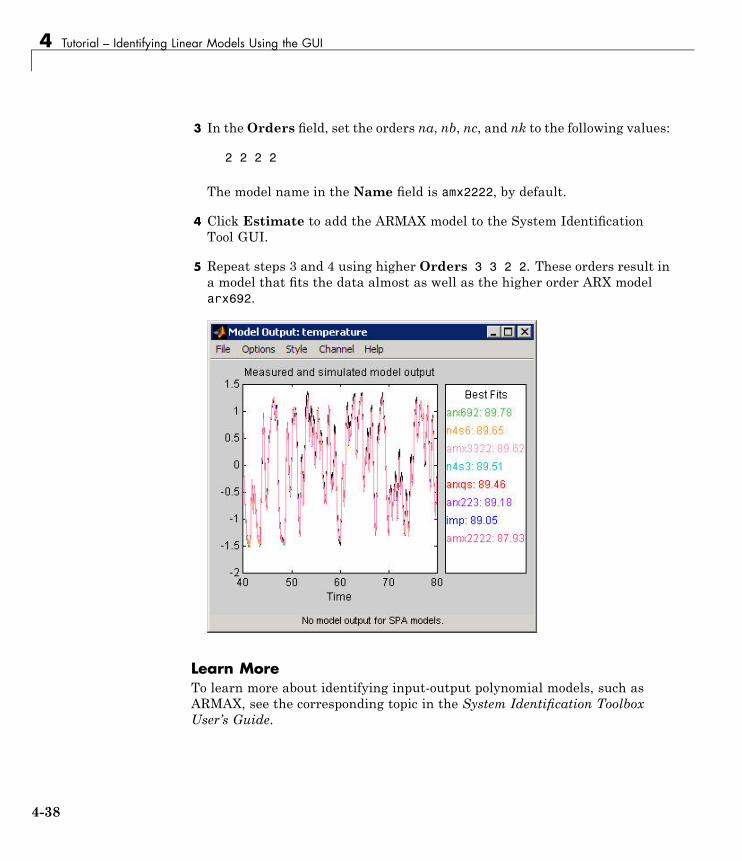
3 In theOrders field, set the orders na, nb, nc, and nk to the following values:
2 2 2 2
The model name in the Name field is amx2222, by default.
4 Click Estimate to add the ARMAX model to the System IdentificationTool GUI.
5 Repeat steps 3 and 4 using higher Orders 3 3 2 2. These orders result ina model that fits the data almost as well as the higher order ARX modelarx692.
Learn MoreTo learn more about identifying input-output polynomial models, such asARMAX, see the corresponding topic in the System Identification ToolboxUser’s Guide.
4-38
Estimating Accurate Linear Models
Choosing the Best ModelYou can compare models to choose the model with the best performance.
You must have already estimated the models, as described in “EstimatingAccurate Linear Models” on page 4-30.
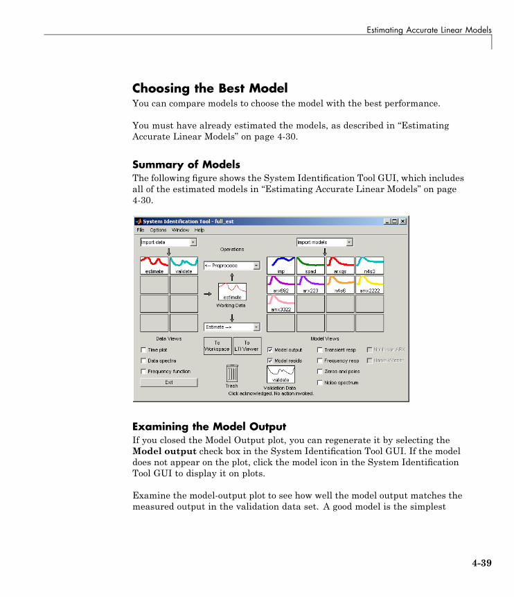
Summary of ModelsThe following figure shows the System Identification Tool GUI, which includesall of the estimated models in “Estimating Accurate Linear Models” on page4-30.
Examining the Model OutputIf you closed the Model Output plot, you can regenerate it by selecting theModel output check box in the System Identification Tool GUI. If the modeldoes not appear on the plot, click the model icon in the System IdentificationTool GUI to display it on plots.
Examine the model-output plot to see how well the model output matches themeasured output in the validation data set. A good model is the simplest
4-39
4 Tutorial – Identifying Linear Models Using the GUI
model that best describes the dynamics and successfully simulates or predictsthe output for different inputs.
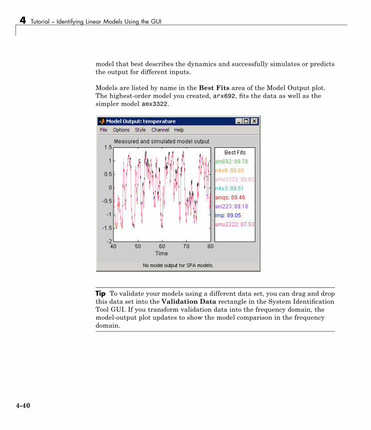
Models are listed by name in the Best Fits area of the Model Output plot.The highest-order model you created, arx692, fits the data as well as thesimpler model amx3322.
Tip To validate your models using a different data set, you can drag and dropthis data set into the Validation Data rectangle in the System IdentificationTool GUI. If you transform validation data into the frequency domain, themodel-output plot updates to show the model comparison in the frequencydomain.
4-40
Estimating Accurate Linear Models
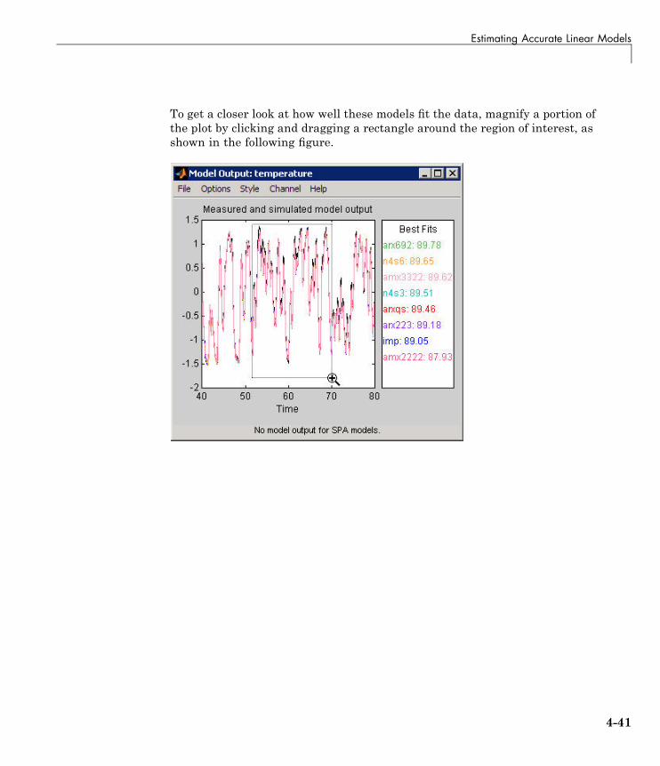
To get a closer look at how well these models fit the data, magnify a portion ofthe plot by clicking and dragging a rectangle around the region of interest, asshown in the following figure.
4-41
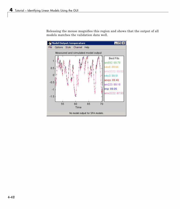
4 Tutorial – Identifying Linear Models Using the GUI
Releasing the mouse magnifies this region and shows that the output of allmodels matches the validation data well.
4-42
Viewing Model Parameters
Viewing Model Parameters
In this section...
“Viewing Model Parameter Values” on page 4-43“Viewing Parameter Uncertainties” on page 4-46
Viewing Model Parameter ValuesYou can view the numerical parameter values for each estimated model.
You must have already estimated the models, as described in “EstimatingAccurate Linear Models” on page 4-30.
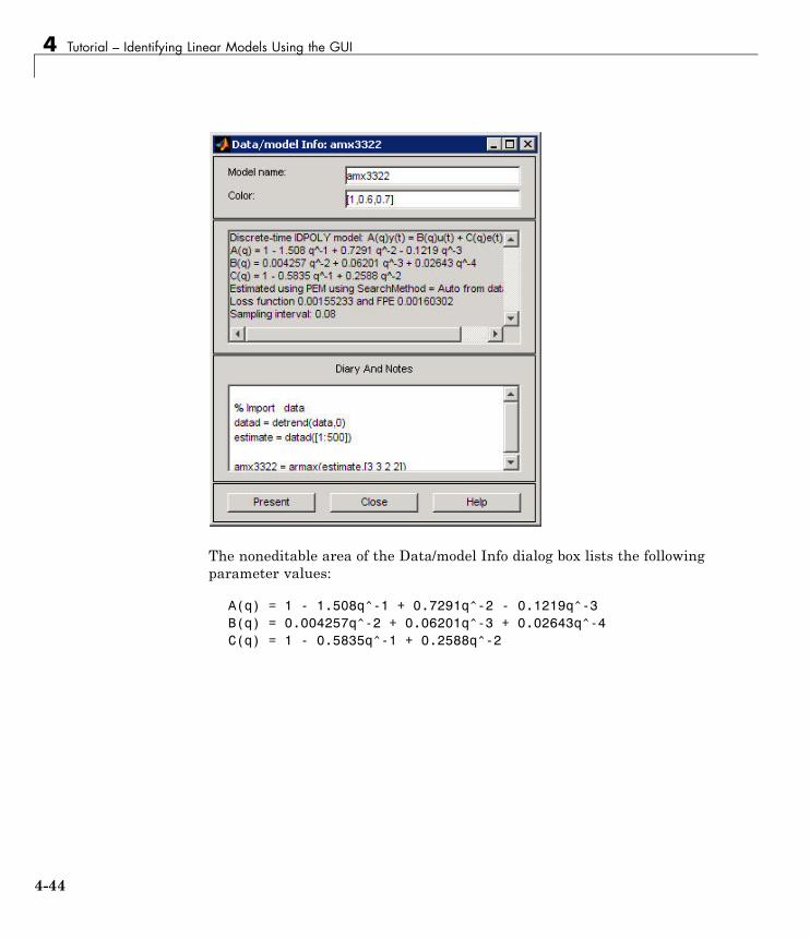
To view the parameter values of the model amx3322, right-click the model iconin the System Identification Tool GUI. The Data/model Info dialog box opens.
4-43
4 Tutorial – Identifying Linear Models Using the GUI
The noneditable area of the Data/model Info dialog box lists the followingparameter values:
A(q) = 1 - 1.508q^-1 + 0.7291q^-2 - 0.1219q^-3B(q) = 0.004257q^-2 + 0.06201q^-3 + 0.02643q^-4C(q) = 1 - 0.5835q^-1 + 0.2588q^-2
4-44
Viewing Model Parameters
These parameter values correspond to the following difference equation foryour system:
y t y t y t y t( ) . ( ) . ( ) . ( ).
− − + − − − =1 508 1 0 7291 2 0 1219 30 004257 uu t u t u te t e t
( ) . ( ) . ( )( ) . (
− + − + − +− −
2 0 06201 3 0 02643 40 5835 11 0 2588 2) . ( )+ −e t
Note The coefficient of u(t-2) is not significantly different from zero. Thislack of difference explains why delay values of both 2 and 3 give good results.
Parameter values appear in the following format:
A q a q a q
B q b q b q
C q c q
nana
nknb
nb nk
( )
( )
( )
= + + +
= + +
= +
− −
− − − +
1
1
11
11
1
…
…−− −+ +1 … c qnc
nc
The parameters appear in the ARMAX model structure, as follows:
A q y t B q u t C q e t( ) ( ) ( ) ( ) ( ) ( )= +
which corresponds to this general difference equation:
y t a y t a y t n
u t n b u t nna a
k nb k
( ) ( ) ( )( ) (
+ − + + − =− + + − −
1 1 …… b1 nn
e t c e t c e t nb
nc c
+ ++ − + + −
111
)( ) ( ) ( ) …
y(t) represents the output at time t, u(t) represents the input at time t, na isthe number of poles for the dynamic model, nb is the number of zeros plus 1, ncis the number of poles for the disturbance model, nk is the number of samplesbefore the input affects output of the system (called the delay or dead time ofthe model), and e(t) is the white-noise disturbance.
4-45
4 Tutorial – Identifying Linear Models Using the GUI
Viewing Parameter UncertaintiesYou can view parameter uncertainties of estimated models.
You must have already estimated the models, as described in “EstimatingAccurate Linear Models” on page 4-30.
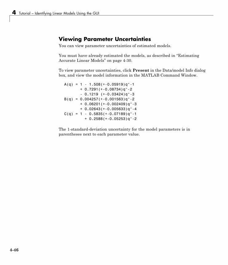
To view parameter uncertainties, click Present in the Data/model Info dialogbox, and view the model information in the MATLAB Command Window.
A(q) = 1 - 1.508(+-0.05919)q^-1+ 0.7291(+-0.08734)q^-2- 0.1219 (+-0.03424)q^-3
B(q) = 0.004257(+-0.001563)q^-2+ 0.06201(+-0.002409)q^-3+ 0.02643(+-0.005633)q^-4
C(q) = 1 - 0.5835(+-0.07189)q^-1+ 0.2588(+-0.05253)q^-2
The 1-standard-deviation uncertainty for the model parameters is inparentheses next to each parameter value.
4-46
Exporting the Model to the MATLAB® Workspace
Exporting the Model to the MATLAB WorkspaceThe models you create in the System Identification Tool GUI are notautomatically available in the MATLAB workspace. To make a modelavailable to other toolboxes, the Simulink software, and the SystemIdentification Toolbox commands, you must export your model from theSystem Identification Tool to the MATLAB workspace. For example, if themodel is a plant that requires a controller, you can import the model from theMATLAB workspace into the Control System Toolbox product.
You must have already estimated the models, as described in “EstimatingAccurate Linear Models” on page 4-30.
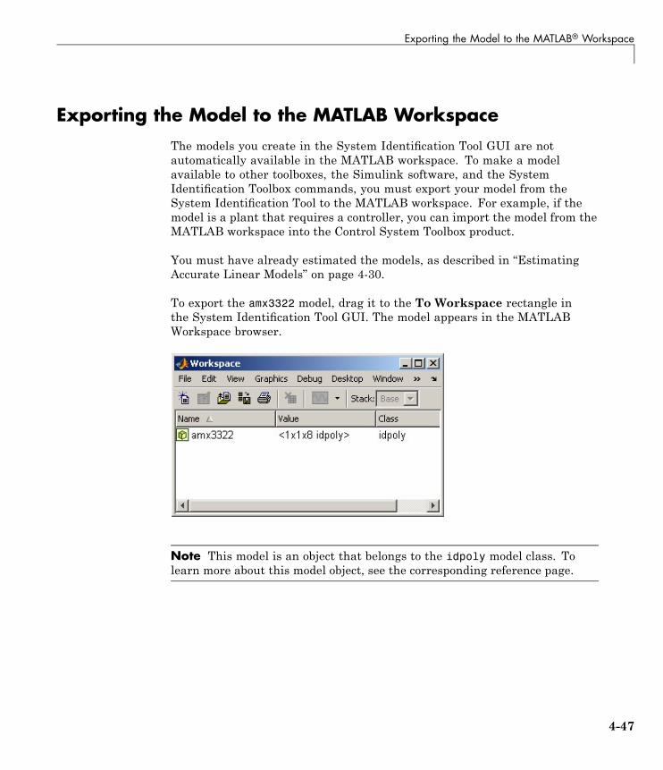
To export the amx3322 model, drag it to the To Workspace rectangle inthe System Identification Tool GUI. The model appears in the MATLABWorkspace browser.
Note This model is an object that belongs to the idpoly model class. Tolearn more about this model object, see the corresponding reference page.
4-47
4 Tutorial – Identifying Linear Models Using the GUI
After the model is in the MATLAB workspace, you can perform otheroperations on the model. For example, if you have the Control System Toolboxproduct installed, you might transform the model to a state-space LTI objectusing:
ss_model=ss(amx3322)
You can extract the dynamic model and ignore the noise model using thefollowing command:
ss_model=ss_model('m')
4-48
Exporting the Model to the LTI Viewer
Exporting the Model to the LTI ViewerIf you have the Control System Toolbox product installed on your computer,the To LTI Viewer rectangle appears in the System Identification Tool GUI.
The LTI Viewer is a graphical user interface for viewing and manipulatingthe response plots of linear models. It displays the following plots:
• Step- and impulse-response
• Bode, Nyquist, and Nichols
• Frequency-response singular values
• Pole/zero
• Response to general input signals
• Unforced response starting from given initial states (only for state-spacemodels)
To plot a model in the LTI Viewer, drag and drop the model icon to the ToLTI Viewer rectangle in the System Identification Tool GUI.
For more information about working with plots in the LTI Viewer, see theControl System Toolbox documentation.
4-49

4 Tutorial – Identifying Linear Models Using the GUI
4-50
5
Tutorial – IdentifyingLow-Order TransferFunctions (Process Models)Using the GUI
• “About This Tutorial” on page 5-2
• “What Is a Continuous-Time Process Model?” on page 5-4
• “Preparing Data for System Identification” on page 5-5
• “Estimating a Second-Order Transfer Function (Process Model) withComplex Poles” on page 5-13
• “Estimating a Transfer Function with a Noise Model” on page 5-22
• “Viewing Model Parameters” on page 5-30
• “Exporting the Model to the MATLAB Workspace” on page 5-33
• “Simulating a System Identification Toolbox Model in Simulink Software”on page 5-34
5 Tutorial – Identifying Low-Order Transfer Functions (Process Models) Using the GUI
About This Tutorial
In this section...
“Objectives” on page 5-2“Data Description” on page 5-3
ObjectivesEstimate and validate simple, continuous-time transfer functions fromsingle-input/single-output (SISO) data to find the one that best describesthe system dynamics.
After completing this tutorial, you will be able to accomplish the followingtasks using the System Identification Tool GUI:
• Import data objects from the MATLAB workspace into the GUI.
• Plot and process the data.
• Estimate and validate low-order, continuous-time models from the data.
• Export models to the MATLAB workspace.
• Simulate the model using Simulink software.
Note This tutorial uses time-domain data to demonstrate how youcan estimate linear models. The same workflow applies to fittingfrequency-domain data.
5-2
About This Tutorial
Data DescriptionThis tutorial uses the data file proc_data.mat, which contains 200 samplesof simulated single-input/single-output (SISO) time-domain data. The inputis a random binary signal that oscillates between -1 and 1. White noise(corresponding to a load disturbance) is added to the input with a standarddeviation of 0.2, which results in a signal-to-noise ratio of about 20 dB. Thisdata is simulated using a second-order system with underdamped modes(complex poles) and a peak response at 1 rad/s:
G ss s
e s( ).
=+ +
−1
1 0 2 22
The sampling interval of the simulation is 1 second.
5-3
5 Tutorial – Identifying Low-Order Transfer Functions (Process Models) Using the GUI
What Is a Continuous-Time Process Model?Continuous-time process models are low-order transfer functions that describethe system dynamics using static gain, a time delay before the system outputresponds to the input, and characteristic time constants associated with polesand zeros. Such models are popular in the industry and are often used fortuning PID controllers, for example. Process model parameters have physicalsignificance.
You can specify different process model structures by varying the number ofpoles, adding an integrator, or including a time delay or a zero. The highestprocess model order you can specify in this toolbox is three, and the poles canbe real or complex (underdamped modes).
In general, a linear system is characterized by a transfer function G, which isan operator that takes the input u to the output y:
y Gu=
For a continuous-time system, G relates the Laplace transforms of the inputU(s) and the output Y(s), as follows:
Y s G s U s( ) ( ) ( )=
In this tutorial, you estimate G using different process-model structures.
For example, the following model structure is a first-order, continuous-timemodel, where K is the static gain, Tp1 is a time constant, and Td is theinput-to-output delay:
G sKsT
ep
sTd( ) =+
−1 1
5-4
Preparing Data for System Identification
Preparing Data for System Identification
In this section...
“Loading Data into the MATLAB Workspace” on page 5-5“Opening the System Identification Tool GUI” on page 5-5“Importing Data Objects into the System Identification Tool” on page 5-6“Plotting and Processing Data” on page 5-9
Loading Data into the MATLAB WorkspaceLoad the data data in proc_data.mat by typing the following command in theMATLAB Command Window:
load proc_data
This command loads the data into the MATLAB workspace as the dataobject z. For more information about iddata objects, see the correspondingreference page.
Opening the System Identification Tool GUITo open the System Identification Tool GUI, type the following commandMATLAB Command Window:
ident
5-5
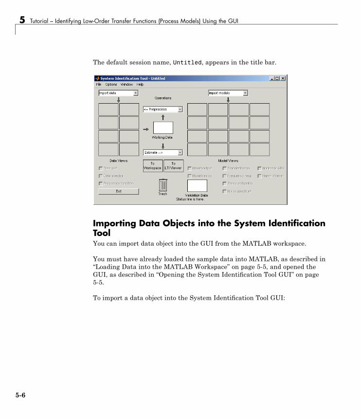
5 Tutorial – Identifying Low-Order Transfer Functions (Process Models) Using the GUI
The default session name, Untitled, appears in the title bar.
Importing Data Objects into the System IdentificationToolYou can import data object into the GUI from the MATLAB workspace.
You must have already loaded the sample data into MATLAB, as described in“Loading Data into the MATLAB Workspace” on page 5-5, and opened theGUI, as described in “Opening the System Identification Tool GUI” on page5-5.
To import a data object into the System Identification Tool GUI:
5-6
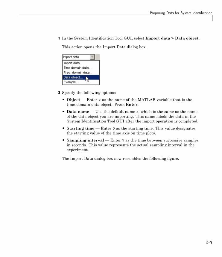
Preparing Data for System Identification
1 In the System Identification Tool GUI, select Import data > Data object.
This action opens the Import Data dialog box.
2 Specify the following options:
• Object — Enter z as the name of the MATLAB variable that is thetime-domain data object. Press Enter.
• Data name— Use the default name z, which is the same as the nameof the data object you are importing. This name labels the data in theSystem Identification Tool GUI after the import operation is completed.
• Starting time — Enter 0 as the starting time. This value designatesthe starting value of the time axis on time plots.
• Sampling interval— Enter 1 as the time between successive samplesin seconds. This value represents the actual sampling interval in theexperiment.
The Import Data dialog box now resembles the following figure.
5-7
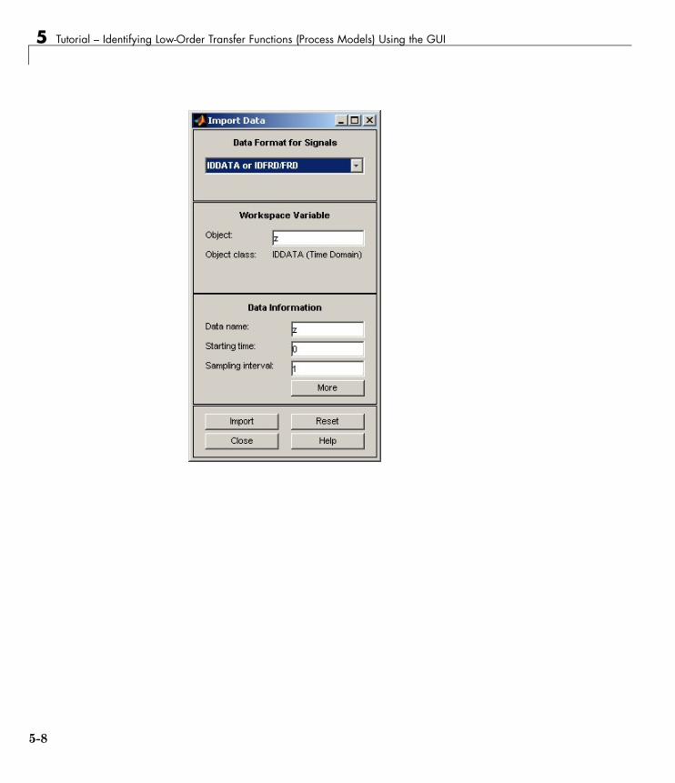
5 Tutorial – Identifying Low-Order Transfer Functions (Process Models) Using the GUI
5-8
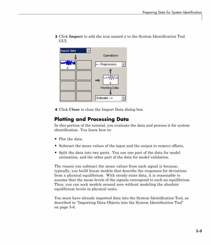
Preparing Data for System Identification
3 Click Import to add the icon named z to the System Identification ToolGUI.
4 Click Close to close the Import Data dialog box.
Plotting and Processing DataIn this portion of the tutorial, you evaluate the data and process it for systemidentification. You learn how to:
• Plot the data.
• Subtract the mean values of the input and the output to remove offsets.
• Split the data into two parts. You use one part of the data for modelestimation, and the other part of the data for model validation.
The reason you subtract the mean values from each signal is because,typically, you build linear models that describe the responses for deviationsfrom a physical equilibrium. With steady-state data, it is reasonable toassume that the mean levels of the signals correspond to such an equilibrium.Thus, you can seek models around zero without modeling the absoluteequilibrium levels in physical units.
You must have already imported data into the System Identification Tool, asdescribed in “Importing Data Objects into the System Identification Tool”on page 5-6.
5-9
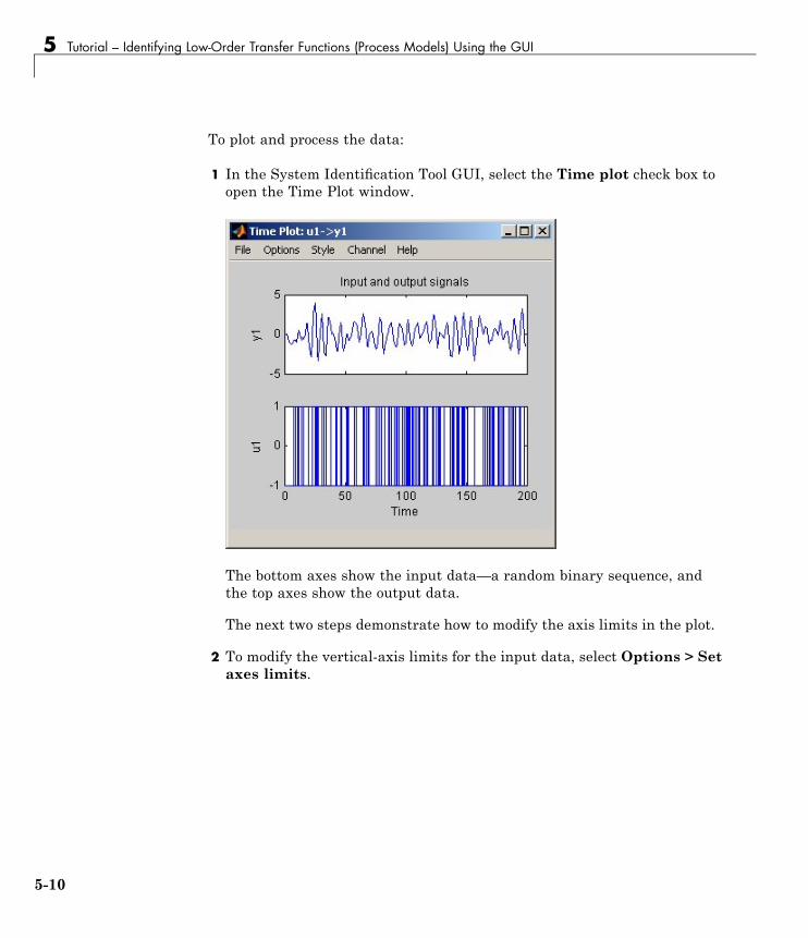
5 Tutorial – Identifying Low-Order Transfer Functions (Process Models) Using the GUI
To plot and process the data:
1 In the System Identification Tool GUI, select the Time plot check box toopen the Time Plot window.
The bottom axes show the input data—a random binary sequence, andthe top axes show the output data.
The next two steps demonstrate how to modify the axis limits in the plot.
2 To modify the vertical-axis limits for the input data, select Options > Setaxes limits.
5-10
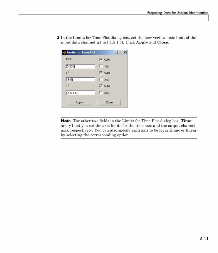
Preparing Data for System Identification
3 In the Limits for Time Plot dialog box, set the new vertical axis limit of theinput data channel u1 to [-1.5 1.5]. Click Apply and Close.
Note The other two fields in the Limits for Time Plot dialog box, Timeand y1, let you set the axis limits for the time axis and the output channelaxis, respectively. You can also specify each axis to be logarithmic or linearby selecting the corresponding option.
5-11
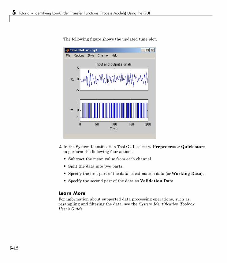
5 Tutorial – Identifying Low-Order Transfer Functions (Process Models) Using the GUI
The following figure shows the updated time plot.
4 In the System Identification Tool GUI, select <–Preprocess > Quick startto perform the following four actions:
• Subtract the mean value from each channel.
• Split the data into two parts.
• Specify the first part of the data as estimation data (orWorking Data).
• Specify the second part of the data as Validation Data.
Learn MoreFor information about supported data processing operations, such asresampling and filtering the data, see the System Identification ToolboxUser’s Guide.
5-12
Estimating a Second-Order Transfer Function (Process Model) with Complex Poles
Estimating a Second-Order Transfer Function (ProcessModel) with Complex Poles
In this section...
“Estimating a Second-Order Transfer Function Using Default Settings”on page 5-13“Tips for Specifying Known Parameters” on page 5-18“Validating the Model” on page 5-18
Estimating a Second-Order Transfer Function UsingDefault SettingsIn this portion of the tutorial, you estimate models with this structure:
G sK
T s T se
w w
T sd( ) =+ +( )
−
1 2 2 2ξ
You must have already processed the data for estimation, as described in“Plotting and Processing Data” on page 5-9.
To identify a second-order transfer function:
5-13
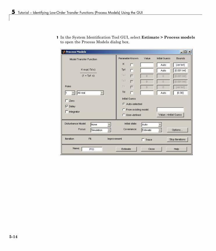
5 Tutorial – Identifying Low-Order Transfer Functions (Process Models) Using the GUI
1 In the System Identification Tool GUI, select Estimate > Process modelsto open the Process Models dialog box.
5-14
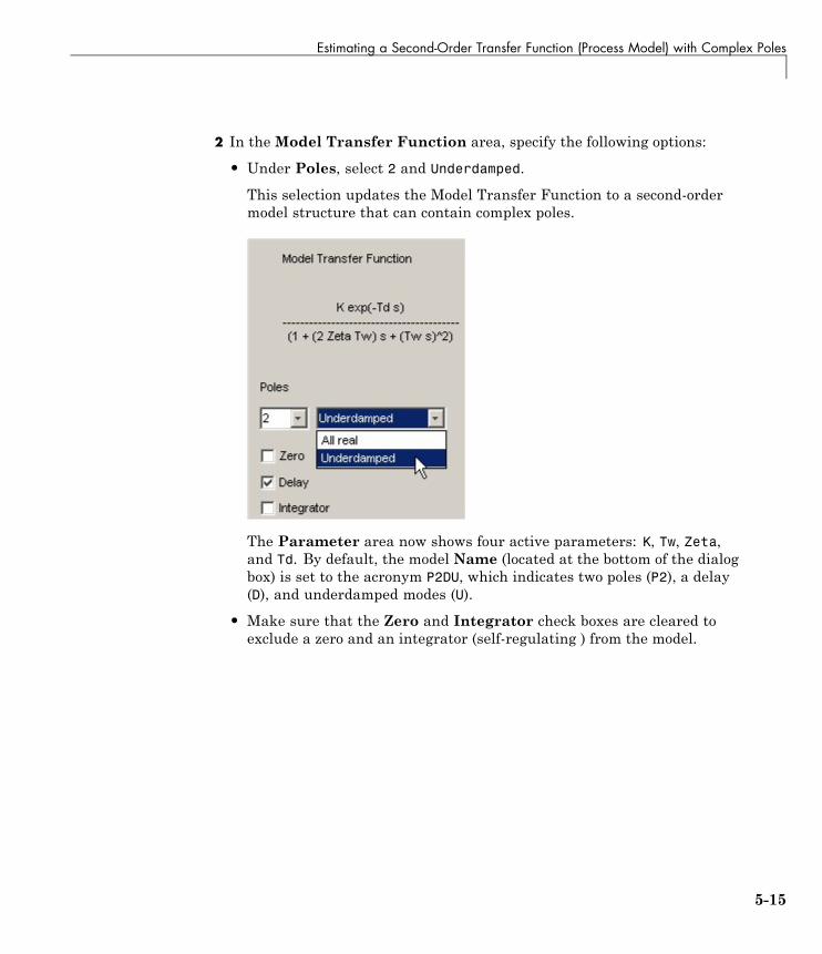
Estimating a Second-Order Transfer Function (Process Model) with Complex Poles
2 In theModel Transfer Function area, specify the following options:
• Under Poles, select 2 and Underdamped.
This selection updates the Model Transfer Function to a second-ordermodel structure that can contain complex poles.
The Parameter area now shows four active parameters: K, Tw, Zeta,and Td. By default, the model Name (located at the bottom of the dialogbox) is set to the acronym P2DU, which indicates two poles (P2), a delay(D), and underdamped modes (U).
• Make sure that the Zero and Integrator check boxes are cleared toexclude a zero and an integrator (self-regulating ) from the model.
5-15
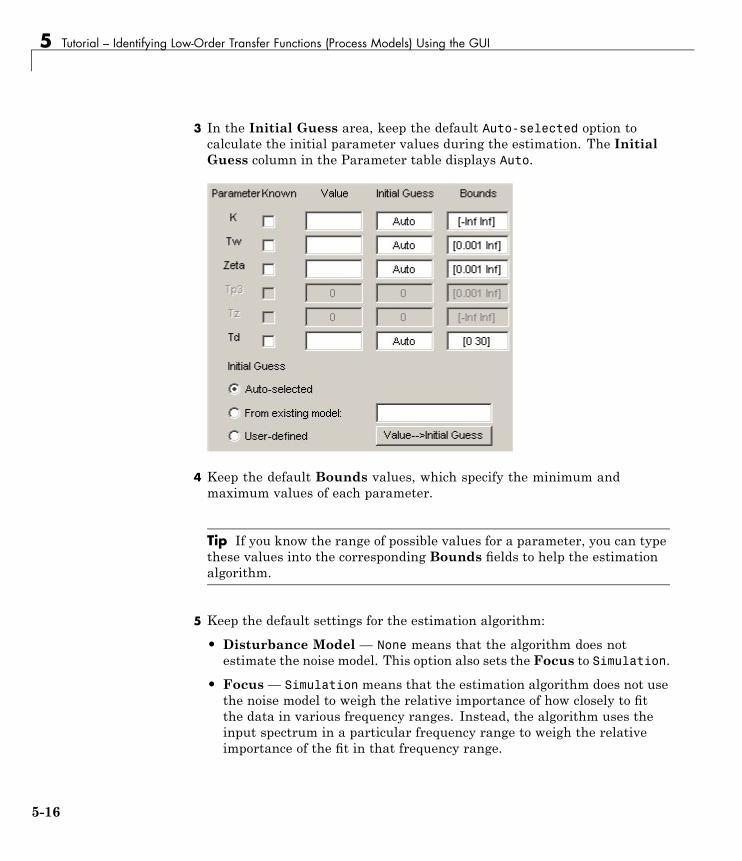
5 Tutorial – Identifying Low-Order Transfer Functions (Process Models) Using the GUI
3 In the Initial Guess area, keep the default Auto-selected option tocalculate the initial parameter values during the estimation. The InitialGuess column in the Parameter table displays Auto.
4 Keep the default Bounds values, which specify the minimum andmaximum values of each parameter.
Tip If you know the range of possible values for a parameter, you can typethese values into the corresponding Bounds fields to help the estimationalgorithm.
5 Keep the default settings for the estimation algorithm:
• Disturbance Model — None means that the algorithm does notestimate the noise model. This option also sets the Focus to Simulation.
• Focus— Simulation means that the estimation algorithm does not usethe noise model to weigh the relative importance of how closely to fitthe data in various frequency ranges. Instead, the algorithm uses theinput spectrum in a particular frequency range to weigh the relativeimportance of the fit in that frequency range.
5-16
Estimating a Second-Order Transfer Function (Process Model) with Complex Poles
Tip The Simulation setting is optimized for identifying models thatyou plan to use for output simulation. If you plan to use your modelfor output prediction or control applications, or to improve parameterestimates using a noise model, select Prediction.
• Initial state — Auto means that the algorithm analyzes the dataand chooses the optimum method for handling the initial state of thesystem. If you get poor results, you might try setting a specific methodfor handling initial states, rather than choosing it automatically.
• Covariance— Estimatemeans that the algorithm computes parameteruncertainties that display as model confidence regions on plots.
6 Click Estimate. This selection adds the model P2DU to the SystemIdentification Tool GUI.
5-17
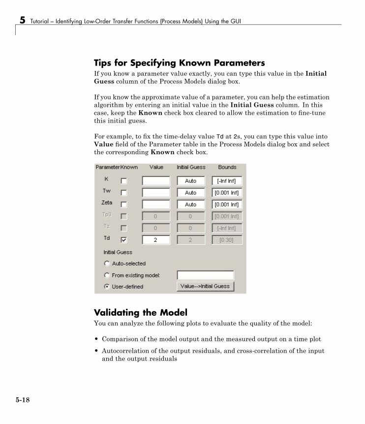
5 Tutorial – Identifying Low-Order Transfer Functions (Process Models) Using the GUI
Tips for Specifying Known ParametersIf you know a parameter value exactly, you can type this value in the InitialGuess column of the Process Models dialog box.
If you know the approximate value of a parameter, you can help the estimationalgorithm by entering an initial value in the Initial Guess column. In thiscase, keep the Known check box cleared to allow the estimation to fine-tunethis initial guess.
For example, to fix the time-delay value Td at 2s, you can type this value intoValue field of the Parameter table in the Process Models dialog box and selectthe corresponding Known check box.
Validating the ModelYou can analyze the following plots to evaluate the quality of the model:
• Comparison of the model output and the measured output on a time plot
• Autocorrelation of the output residuals, and cross-correlation of the inputand the output residuals
5-18
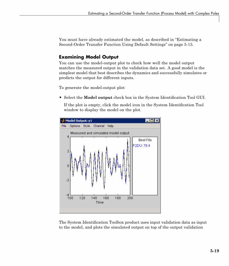
Estimating a Second-Order Transfer Function (Process Model) with Complex Poles
You must have already estimated the model, as described in “Estimating aSecond-Order Transfer Function Using Default Settings” on page 5-13.
Examining Model OutputYou can use the model-output plot to check how well the model outputmatches the measured output in the validation data set. A good model is thesimplest model that best describes the dynamics and successfully simulates orpredicts the output for different inputs.
To generate the model-output plot:
• Select theModel output check box in the System Identification Tool GUI.
If the plot is empty, click the model icon in the System Identification Toolwindow to display the model on the plot.
The System Identification Toolbox product uses input validation data as inputto the model, and plots the simulated output on top of the output validation
5-19
5 Tutorial – Identifying Low-Order Transfer Functions (Process Models) Using the GUI
data. The preceding plot shows that the model output agrees well with thevalidation-data output.
The Best Fits area of the Model Output plot shows the agreement (in percent)between the model output and the validation-data output.
Recall that the data was simulated using the following second-order systemwith underdamped modes (complex poles), as described in “Data Description”on page 5-3, and has a peak response at 1 rad/s:
G ss s
e s( ).
=+ +
−1
1 0 2 22
Because the data includes noise at the input during the simulation, theestimated model cannot exactly reproduce the model used to simulate thedata.
Examining Model ResidualsYou can validate a model by checking the behavior of its residuals.
To generate a Residual Analysis plot, select the Model resids check box inthe System Identification Tool GUI.
5-20
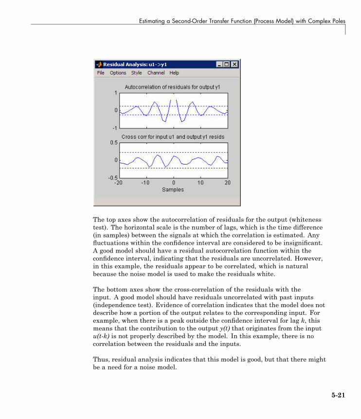
Estimating a Second-Order Transfer Function (Process Model) with Complex Poles
The top axes show the autocorrelation of residuals for the output (whitenesstest). The horizontal scale is the number of lags, which is the time difference(in samples) between the signals at which the correlation is estimated. Anyfluctuations within the confidence interval are considered to be insignificant.A good model should have a residual autocorrelation function within theconfidence interval, indicating that the residuals are uncorrelated. However,in this example, the residuals appear to be correlated, which is naturalbecause the noise model is used to make the residuals white.
The bottom axes show the cross-correlation of the residuals with theinput. A good model should have residuals uncorrelated with past inputs(independence test). Evidence of correlation indicates that the model does notdescribe how a portion of the output relates to the corresponding input. Forexample, when there is a peak outside the confidence interval for lag k, thismeans that the contribution to the output y(t) that originates from the inputu(t-k) is not properly described by the model. In this example, there is nocorrelation between the residuals and the inputs.
Thus, residual analysis indicates that this model is good, but that there mightbe a need for a noise model.
5-21
5 Tutorial – Identifying Low-Order Transfer Functions (Process Models) Using the GUI
Estimating a Transfer Function with a Noise Model
In this section...
“Estimating a Second-Order Transfer Function with Complex Poles andNoise” on page 5-22“Validating the Models” on page 5-24
Estimating a Second-Order Transfer Function withComplex Poles and NoiseIn this portion of the tutorial, you estimate a second-order transfer functionand include a noise model. By including a noise model, you optimize theestimation results for prediction application.
You must have already estimated the model, as described in “Estimating aSecond-Order Transfer Function Using Default Settings” on page 5-13.
To estimate a second-order transfer function with noise:
1 If the Process Models dialog box is not open, select Estimate > Processmodels in the System Identification Tool GUI. This action opens theProcess Models dialog box.
5-22
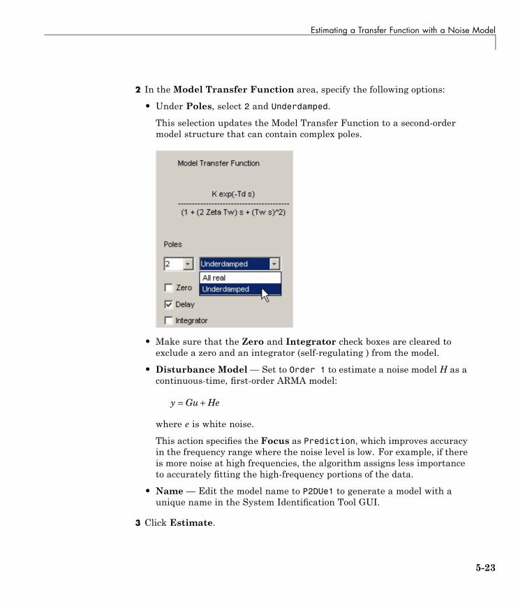
Estimating a Transfer Function with a Noise Model
2 In theModel Transfer Function area, specify the following options:
• Under Poles, select 2 and Underdamped.
This selection updates the Model Transfer Function to a second-ordermodel structure that can contain complex poles.
• Make sure that the Zero and Integrator check boxes are cleared toexclude a zero and an integrator (self-regulating ) from the model.
• Disturbance Model— Set to Order 1 to estimate a noise model H as acontinuous-time, first-order ARMA model:
y Gu He= +
where e is white noise.
This action specifies the Focus as Prediction, which improves accuracyin the frequency range where the noise level is low. For example, if thereis more noise at high frequencies, the algorithm assigns less importanceto accurately fitting the high-frequency portions of the data.
• Name — Edit the model name to P2DUe1 to generate a model with aunique name in the System Identification Tool GUI.
3 Click Estimate.
5-23
5 Tutorial – Identifying Low-Order Transfer Functions (Process Models) Using the GUI
4 In the Process Models dialog box, set the Disturbance Model to Order 2to estimate a second-order noise model.
5 Edit the Name field to P2DUe2 to generate a model with a unique name inthe System Identification Tool GUI.
6 Click Estimate.
Validating the ModelsIn this portion of the tutorial, you evaluate model performance using theModel Output and the Residual Analysis plots.
You must have already estimated the models, as described in “Estimating aSecond-Order Transfer Function Using Default Settings” on page 5-13 and“Estimating a Second-Order Transfer Function with Complex Poles andNoise” on page 5-22.
Comparing the Model Output PlotsTo generate the Model Output plot:
• Select theModel output check box in the System Identification Tool GUI.
If the plot is empty, click the model icons in the System Identification Toolwindow to display these models on the plot.
5-24
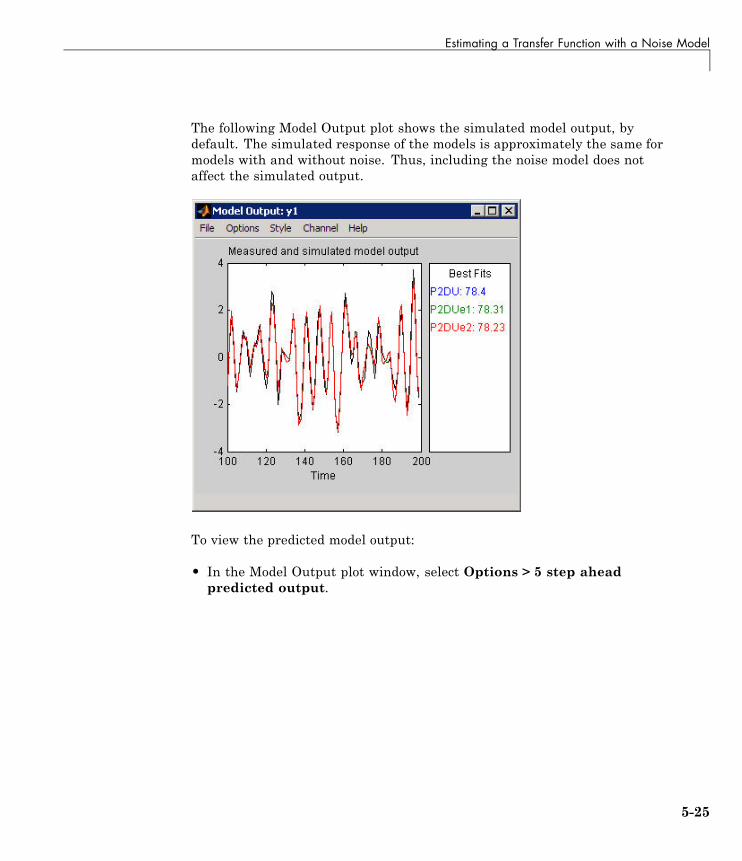
Estimating a Transfer Function with a Noise Model
The following Model Output plot shows the simulated model output, bydefault. The simulated response of the models is approximately the same formodels with and without noise. Thus, including the noise model does notaffect the simulated output.
To view the predicted model output:
• In the Model Output plot window, select Options > 5 step aheadpredicted output.
5-25
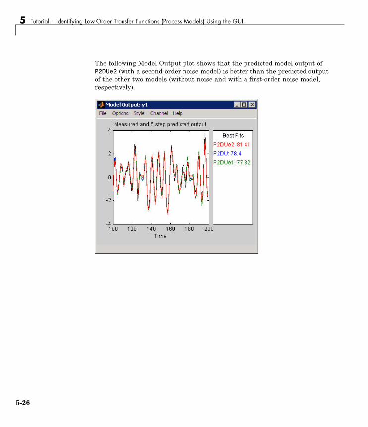
5 Tutorial – Identifying Low-Order Transfer Functions (Process Models) Using the GUI
The following Model Output plot shows that the predicted model output ofP2DUe2 (with a second-order noise model) is better than the predicted outputof the other two models (without noise and with a first-order noise model,respectively).
5-26
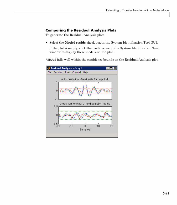
Estimating a Transfer Function with a Noise Model
Comparing the Residual Analysis PlotsTo generate the Residual Analysis plot:
• Select theModel resids check box in the System Identification Tool GUI.
If the plot is empty, click the model icons in the System Identification Toolwindow to display these models on the plot.
P2DUe2 falls well within the confidence bounds on the Residual Analysis plot.
5-27
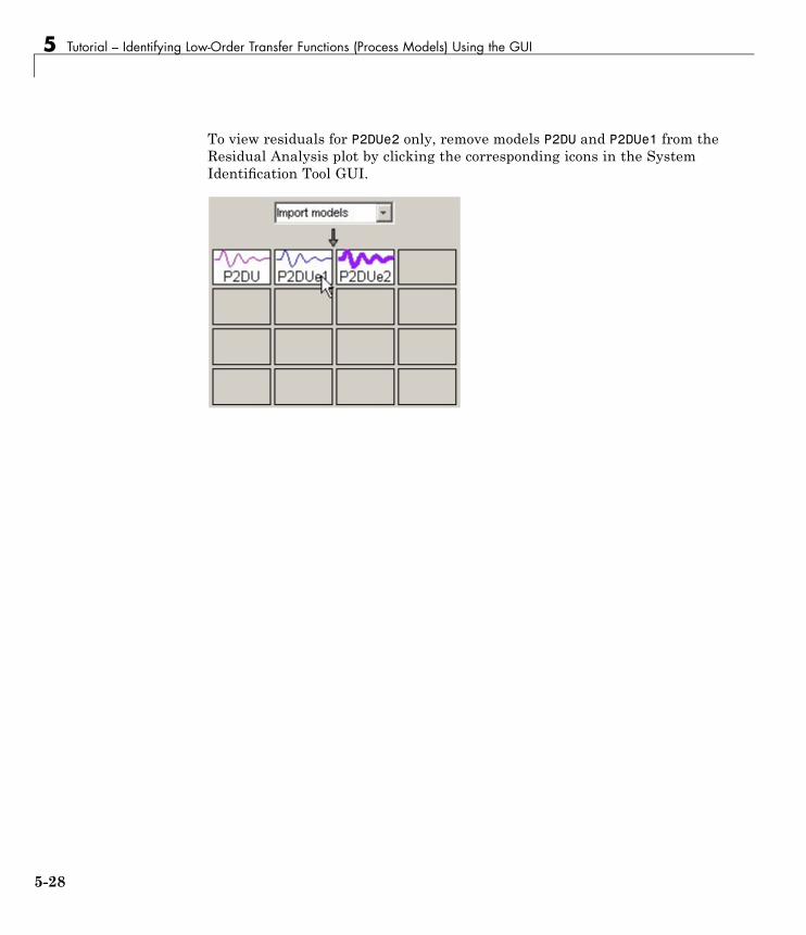
5 Tutorial – Identifying Low-Order Transfer Functions (Process Models) Using the GUI
To view residuals for P2DUe2 only, remove models P2DU and P2DUe1 from theResidual Analysis plot by clicking the corresponding icons in the SystemIdentification Tool GUI.
5-28

Estimating a Transfer Function with a Noise Model
The Residual Analysis plot updates, as shown in the following figure.
The whiteness test for P2DUe2 shows that the residuals are uncorrelated, andthe independence test shows no correlation between the residuals and theinputs. These tests indicate that P2DUe2 is a good model.
5-29
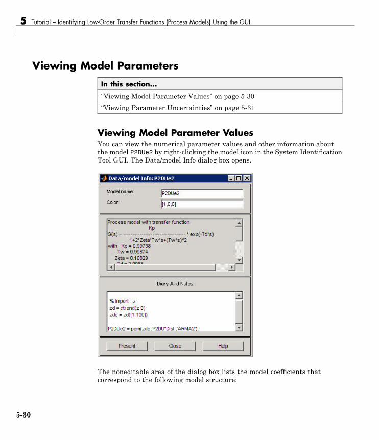
5 Tutorial – Identifying Low-Order Transfer Functions (Process Models) Using the GUI
Viewing Model Parameters
In this section...
“Viewing Model Parameter Values” on page 5-30“Viewing Parameter Uncertainties” on page 5-31
Viewing Model Parameter ValuesYou can view the numerical parameter values and other information aboutthe model P2DUe2 by right-clicking the model icon in the System IdentificationTool GUI. The Data/model Info dialog box opens.
The noneditable area of the dialog box lists the model coefficients thatcorrespond to the following model structure:
5-30
Viewing Model Parameters
G sK
T s T se
w w
T sd( ) =+ +( )
−
1 2 2 2ξ
For the model P2DUe2:
• Kp is 0.99783.
• Tw is 0.99874.
• Zeta is 0.10829.
• Td is 2.0058.
These coefficients agree with the model used to simulate the data:
G ss s
e s( ).
=+ +
−1
1 0 2 22
P2DUe2 also includes an additive noise term, where H is a second-order ARMAmodel and e is white noise:
y Gu He= +
The Data/model Info dialog box gives the noise model H as a ratio of twopolynomials, C(s)/D(s), where:
C(s) = s^2 + 2.14(+-0.08596)s + 1.175(+-0.3083)D(s) = s^2 + 0.2427(+-0.08213)s + 0.61(+-0.07577)
The 1-standard-deviation uncertainty for the model parameters is inparentheses next to each parameter value.
Viewing Parameter UncertaintiesTo view parameter uncertainties for the system transfer function, clickPresent in the Data/model Info dialog box, and view the information in theMATLAB Command Window.
Kp = 0.99738+-0.01951Tw = 0.99874+-0.0037075
5-31
5 Tutorial – Identifying Low-Order Transfer Functions (Process Models) Using the GUI
Zeta = 0.10829+-0.0040998Td = 2.0058+-0.002329
The 1-standard-deviation uncertainty for each model parameter follows the+- symbol.
5-32
Exporting the Model to the MATLAB® Workspace
Exporting the Model to the MATLAB WorkspaceYou can perform further analysis on your estimated models from theMATLAB workspace. For example, if the model is a plant that requires acontroller, you can import the model from the MATLAB workspace into theControl System Toolbox product. Furthermore, to simulate your model in theSimulink software (perhaps as part of a larger dynamic system), you canimport this model as a Simulink block.
The models you create in the System Identification Tool GUI are notautomatically available in the MATLAB workspace. To make a modelavailable to other toolboxes, Simulink, and the System Identification Toolboxcommands, you must export your model from the System Identification Toolto the MATLAB workspace.
To export the P2DUe2 model:
• In the System Identification Tool GUI, drag the model icon to the ToWorkspace rectangle. The model now appears in the MATLAB Workspacebrowser.
Note This model is an object of idproc class. Model objects encapsulateall properties of the model. To learn more about this model object, see thecorresponding reference page.
5-33
5 Tutorial – Identifying Low-Order Transfer Functions (Process Models) Using the GUI
Simulating a System Identification Toolbox Model inSimulink Software
In this section...
“Prerequisites for This Tutorial” on page 5-34“Preparing Input Data” on page 5-34“Building the Simulink Model” on page 5-35“Configuring Blocks and Simulation Parameters” on page 5-36“Running the Simulation” on page 5-40
Prerequisites for This TutorialIn this tutorial, you create a simple Simulink model that uses blocks fromthe System Identification Toolbox library to bring the data z and the modelP2DUe2 into Simulink.
To perform the steps in this tutorial, Simulink must be installed on yourcomputer.
Furthermore, you must have already performed the following steps:
• Load the data set, as described in “Loading Data into the MATLABWorkspace” on page 5-5.
• Estimate the second-order process model, as described in “Estimating aSecond-Order Transfer Function with Complex Poles and Noise” on page5-22.
• Export the model to the MATLAB workspace, as described in “Exportingthe Model to the MATLAB Workspace” on page 5-33.
Preparing Input DataUse the input channel of the data set z as input for simulating the modeloutput by typing the following in the MATLAB Command Window:
z_input = z % Creates a new iddata object.z_input.y = [] % Sets the output channel
5-34
Simulating a System Identification Toolbox™ Model in Simulink® Software
% to empty.
Alternatively, you can specify any input signal.
Learn MoreFor more information about representing data signals for systemidentification, see the System Identification Toolbox User’s Guide.
Building the Simulink ModelTo add blocks to a Simulink model:
1 In the MATLAB Command Window, type simulink.
2 Select File > New > Model to open a new model window.
3 In the Simulink Library Browser, select the System IdentificationToolbox library. The right side of the window displays blocks specific tothe System Identification Toolbox product.
Tip Another way to access the System Identification block library is to typeslident in the MATLAB Command Window.
4 Drag the following System Identification Toolbox blocks to the new modelwindow:
• IDDATA Sink block
• IDDATA Source block
• IDMODEL model block
5 In the Simulink Library Browser, select the Simulink > Sinks library,and drag the Scope block to the new model window.
5-35
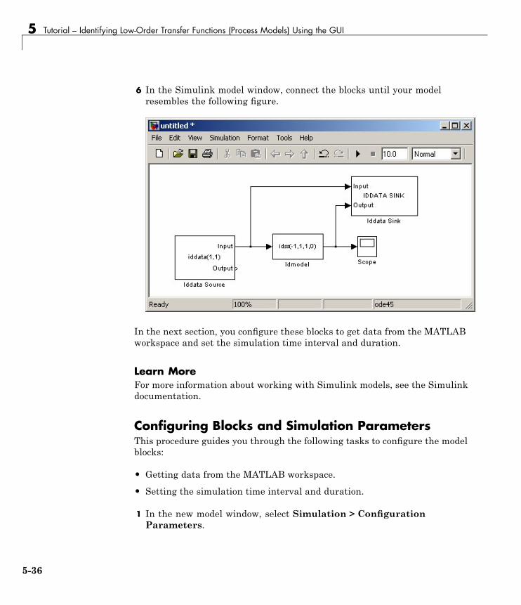
5 Tutorial – Identifying Low-Order Transfer Functions (Process Models) Using the GUI
6 In the Simulink model window, connect the blocks until your modelresembles the following figure.
In the next section, you configure these blocks to get data from the MATLABworkspace and set the simulation time interval and duration.
Learn MoreFor more information about working with Simulink models, see the Simulinkdocumentation.
Configuring Blocks and Simulation ParametersThis procedure guides you through the following tasks to configure the modelblocks:
• Getting data from the MATLAB workspace.
• Setting the simulation time interval and duration.
1 In the new model window, select Simulation > ConfigurationParameters.
5-36
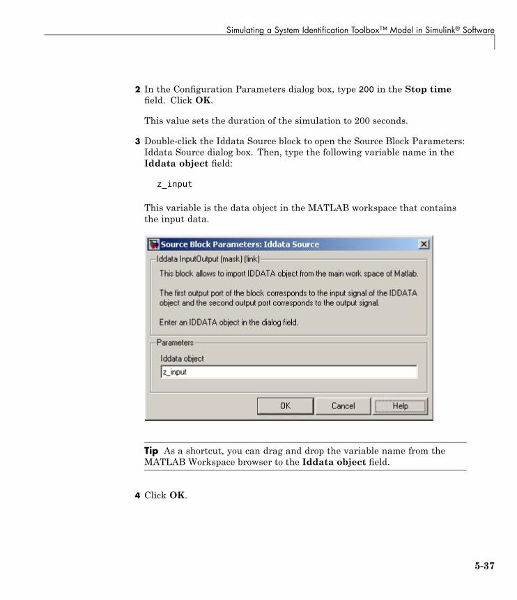
Simulating a System Identification Toolbox™ Model in Simulink® Software
2 In the Configuration Parameters dialog box, type 200 in the Stop timefield. Click OK.
This value sets the duration of the simulation to 200 seconds.
3 Double-click the Iddata Source block to open the Source Block Parameters:Iddata Source dialog box. Then, type the following variable name in theIddata object field:
z_input
This variable is the data object in the MATLAB workspace that containsthe input data.
Tip As a shortcut, you can drag and drop the variable name from theMATLAB Workspace browser to the Iddata object field.
4 Click OK.
5-37
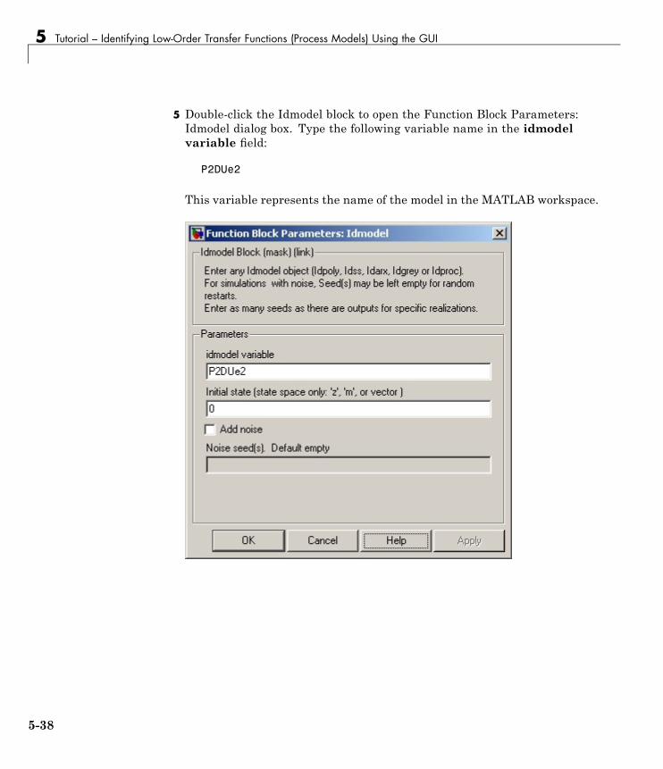
5 Tutorial – Identifying Low-Order Transfer Functions (Process Models) Using the GUI
5 Double-click the Idmodel block to open the Function Block Parameters:Idmodel dialog box. Type the following variable name in the idmodelvariable field:
P2DUe2
This variable represents the name of the model in the MATLAB workspace.
5-38

Simulating a System Identification Toolbox™ Model in Simulink® Software
6 Clear the Add noise check box to exclude noise from the simulation. ClickOK.
When Add noise is selected, Simulink derives the noise amplitude fromthe NoiseVariance property of the model and adds noise to the modelaccordingly. The simulation propagates this noise according to the noisemodel H that was estimated with the system dynamics:
y Gu He= +
7 Double-click the Iddata Sink block to open the Sink Block Parameters:Iddata Sink dialog box. Type the following variable name in the IDDATAName field:
z_sim_out
8 Type 1 in the Sample Time (sec.) field to set the sampling time of theoutput data to match the sampling time of the input data. Click OK.
5-39
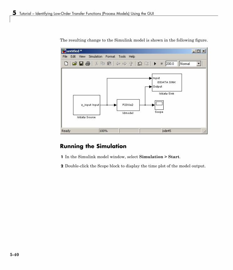
5 Tutorial – Identifying Low-Order Transfer Functions (Process Models) Using the GUI
The resulting change to the Simulink model is shown in the following figure.
Running the Simulation
1 In the Simulink model window, select Simulation > Start.
2 Double-click the Scope block to display the time plot of the model output.
5-40
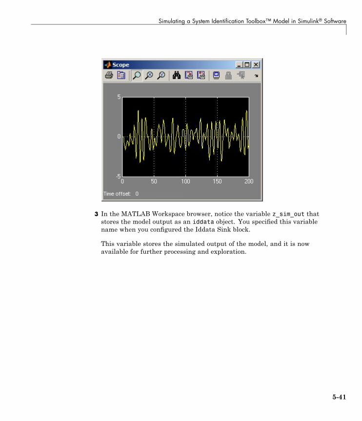
Simulating a System Identification Toolbox™ Model in Simulink® Software
3 In the MATLAB Workspace browser, notice the variable z_sim_out thatstores the model output as an iddata object. You specified this variablename when you configured the Iddata Sink block.
This variable stores the simulated output of the model, and it is nowavailable for further processing and exploration.
5-41

5 Tutorial – Identifying Low-Order Transfer Functions (Process Models) Using the GUI
5-42
6
Tutorial – IdentifyingLinear Models Using theCommand Line
• “About This Tutorial” on page 6-2
• “Preparing Data” on page 6-4
• “Estimating Step- and Frequency-Response Models” on page 6-15
• “Estimating Delays in the Multiple-Input System” on page 6-20
• “Estimating Model Orders Using an ARX Model Structure” on page 6-23
• “Estimating Continuous-Time Transfer Functions (Process Models)” onpage 6-31
• “Estimating Black-Box Polynomial Models” on page 6-42
• “Simulating and Predicting Model Output” on page 6-54
6 Tutorial – Identifying Linear Models Using the Command Line
About This Tutorial
In this section...
“Objectives” on page 6-2“Data Description” on page 6-2
ObjectivesEstimate and validate linear models from multiple-input/single-output(MISO) data to find the one that best describes the system dynamics.
After completing this tutorial, you will be able to accomplish the followingtasks using the command line:
• Create data objects to represent data.
• Plot the data.
• Process data by removing offsets from the input and output signals.
• Estimate and validate linear models from the data.
• Simulate and predict model output.
Note This tutorial uses time-domain data to demonstrate how youcan estimate linear models. The same workflow applies to fittingfrequency-domain data.
Data DescriptionThis tutorial uses the data file co2data.mat, which contains two experimentsof two-input and single-output (MISO) time-domain data from a steady-statethat the operator perturbed from equilibrium values.
In the first experiment, the operator introduced a pulse wave to both inputs.In the second experiment, the operator introduced a pulse wave to the firstinput and a step signal to the second input.
6-2

About This Tutorial
6-3
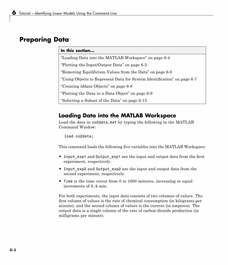
6 Tutorial – Identifying Linear Models Using the Command Line
Preparing Data
In this section...
“Loading Data into the MATLAB Workspace” on page 6-4“Plotting the Input/Output Data” on page 6-5“Removing Equilibrium Values from the Data” on page 6-6“Using Objects to Represent Data for System Identification” on page 6-7“Creating iddata Objects” on page 6-8“Plotting the Data in a Data Object” on page 6-9“Selecting a Subset of the Data” on page 6-13
Loading Data into the MATLAB WorkspaceLoad the data in co2data.mat by typing the following in the MATLABCommand Window:
load co2data;
This command loads the following five variables into the MATLABWorkspace:
• Input_exp1 and Output_exp1 are the input and output data from the firstexperiment, respectively.
• Input_exp2 and Output_exp2 are the input and output data from thesecond experiment, respectively.
• Time is the time vector from 0 to 1000 minutes, increasing in equalincrements of 0.5 min.
For both experiments, the input data consists of two columns of values. Thefirst column of values is the rate of chemical consumption (in kilograms perminute), and the second column of values is the current (in amperes). Theoutput data is a single column of the rate of carbon-dioxide production (inmilligrams per minute).
6-4
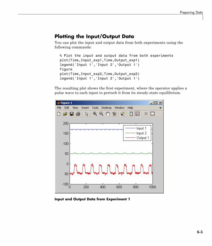
Preparing Data
Plotting the Input/Output DataYou can plot the input and output data from both experiments using thefollowing commands:
% Plot the input and output data from both experimentsplot(Time,Input_exp1,Time,Output_exp1)legend('Input 1','Input 2','Output 1')figureplot(Time,Input_exp2,Time,Output_exp2)legend('Input 1','Input 2','Output 1')
The resulting plot shows the first experiment, where the operator applies apulse wave to each input to perturb it from its steady-state equilibrium.
Input and Output Data from Experiment 1
6-5
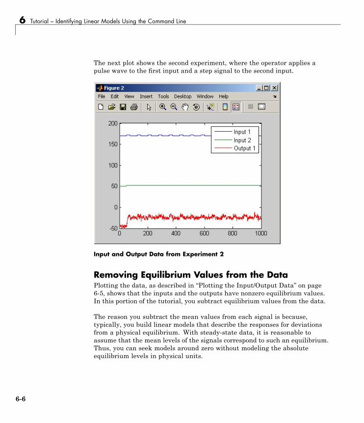
6 Tutorial – Identifying Linear Models Using the Command Line
The next plot shows the second experiment, where the operator applies apulse wave to the first input and a step signal to the second input.
Input and Output Data from Experiment 2
Removing Equilibrium Values from the DataPlotting the data, as described in “Plotting the Input/Output Data” on page6-5, shows that the inputs and the outputs have nonzero equilibrium values.In this portion of the tutorial, you subtract equilibrium values from the data.
The reason you subtract the mean values from each signal is because,typically, you build linear models that describe the responses for deviationsfrom a physical equilibrium. With steady-state data, it is reasonable toassume that the mean levels of the signals correspond to such an equilibrium.Thus, you can seek models around zero without modeling the absoluteequilibrium levels in physical units.
6-6
Preparing Data
Zoom in on the plots to see that the earliest moment when the operatorapplies a disturbance to the inputs occurs after 25 minutes of steady-stateconditions (or after the first 50 samples). Thus, the average value of the first50 samples represents the equilibrium conditions.
Use the following commands to remove the equilibrium values from the inputsand the outputs in both experiments:
% Remove the equilibrium values from inputs% and outputs in both experiments:Input_exp1 = Input_exp1-...
ones(size(Input_exp1,1),1)*mean(Input_exp1(1:50,:));Output_exp1 = Output_exp1-...
mean(Output_exp1(1:50,:));Input_exp2 = Input_exp2-...
ones(size(Input_exp2,1),1)*mean(Input_exp2(1:50,:));Output_exp2 = Output_exp2-...
mean(Output_exp2(1:50,:));
Note The ones command replicates the two mean values, one for each input,in a two-dimensional array.
Using Objects to Represent Data for SystemIdentificationThe System Identification Toolbox data objects, iddata and idfrd,encapsulate both data values and data properties into a single entity. You canuse the System Identification Toolbox commands to conveniently manipulatethese data objects as single entities.
In this portion of the tutorial, you create two iddata objects, one for eachof the two experiments. You use the data from Experiment 1 for modelestimation, and the data from Experiment 2 for model validation. You workwith two independent data sets because you use one data set for modelestimation and the other for model validation.
6-7
6 Tutorial – Identifying Linear Models Using the Command Line
Note When two independent data sets are not available, you can split onedata set into two parts, assuming that each part contains enough informationto adequately represent the system dynamics.
Creating iddata ObjectsYou must have already loaded the sample data into the MATLAB workspace,as described in “Loading Data into the MATLAB Workspace” on page 7-4.
Use these commands to create two data objects, ze and zv:
% Create two data objects, ze and zv.Ts = 0.5; % Sampling interval is 0.5 minze = iddata(Output_exp1,Input_exp1,Ts);zv = iddata(Output_exp2,Input_exp2,Ts);
ze contains data from Experiment 1 and zv contains data from Experiment 2.Ts is the sampling interval.
The iddata constructor requires three arguments for time-domain data andhas the following syntax:
data_obj = iddata(output,input,sampling_interval);
To view the properties of an iddata object, use the get command. Forexample, type this command to get the properties of the estimation data:
get(ze)
To learn more about the properties of this data object, see the iddatareference page.
6-8
Preparing Data
To modify data properties, you can use dot notation or the set command. Forexample, to assign channel names and units that label plot axes, type thefollowing syntax in the MATLAB Command Window:
% Set time units to minutesze.TimeUnit = 'min';% Set names of input channelsze.InputName = {'ConsumptionRate','Current'};% Set units for input variablesze.InputUnit = {'kg/min','A'};% Set name of output channelze.OutputName = 'Production';% Set unit of output channelze.OutputUnit = 'mg/min';
% Set validation data propertieszv.TimeUnit = 'min';zv.InputName = {'ConsumptionRate','Current'};zv.InputUnit = {'kg/min','A'};zv.OutputName = 'Production';zv.OutputUnit = 'mg/min';
You can verify that the InputName property of ze is changed, or “index into”this property, by typing the following syntax:
ze.inputname
Tip Property names, such as InputUnit, are not case sensitive. You can alsoabbreviate property names that start with Input or Output by substituting ufor Input and y for Output in the property name. For example, OutputUnit isequivalent to yunit.
Plotting the Data in a Data ObjectYou can plot iddata objects using the MATLAB plot command:
plot(ze) % Plot the estimation data
6-9
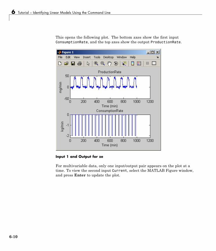
6 Tutorial – Identifying Linear Models Using the Command Line
This opens the following plot. The bottom axes show the first inputConsumptionRate, and the top axes show the output ProductionRate.
Input 1 and Output for ze
For multivariable data, only one input/output pair appears on the plot at atime. To view the second input Current, select the MATLAB Figure window,and press Enter to update the plot.
6-10
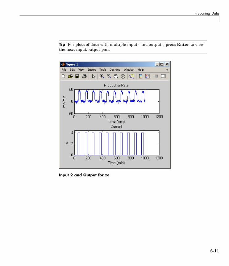
Preparing Data
Tip For plots of data with multiple inputs and outputs, press Enter to viewthe next input/output pair.
Input 2 and Output for ze
6-11

6 Tutorial – Identifying Linear Models Using the Command Line
To plot the validation data in a new MATLAB Figure window, type thefollowing commands in the MATLAB Command Window:
figure % Open a new MATLAB Figure windowplot(zv) % Plot the validation data
Input 1 and Output for zv
6-12
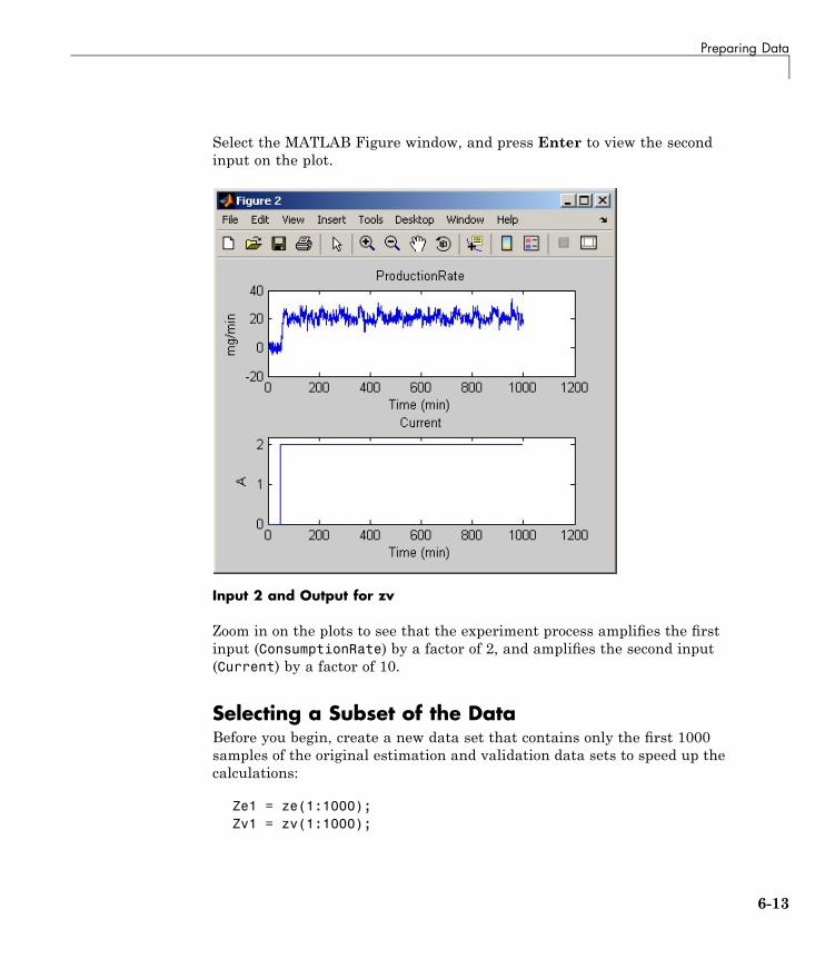
Preparing Data
Select the MATLAB Figure window, and press Enter to view the secondinput on the plot.
Input 2 and Output for zv
Zoom in on the plots to see that the experiment process amplifies the firstinput (ConsumptionRate) by a factor of 2, and amplifies the second input(Current) by a factor of 10.
Selecting a Subset of the DataBefore you begin, create a new data set that contains only the first 1000samples of the original estimation and validation data sets to speed up thecalculations:
Ze1 = ze(1:1000);Zv1 = zv(1:1000);
6-13

6 Tutorial – Identifying Linear Models Using the Command Line
For more information about indexing into iddata objects, see thecorresponding reference page.
6-14
Estimating Step- and Frequency-Response Models
Estimating Step- and Frequency-Response Models
In this section...
“Why Estimate Step- and Frequnecy-Response Models?” on page 6-15“Estimating the Frequency Response” on page 6-15“Estimating the Step Response” on page 6-18
Why Estimate Step- and Frequnecy-ResponseModels?Frequency-response and step-response are nonparametric models that canhelp you understand the dynamic characteristics of your system. Thesemodels are not represented by a compact mathematical formula withadjustable parameters. Instead, they consist of data tables.
In this portion of the tutorial, you estimate these models using the data setze. You must have already created ze, as described in “Creating iddataObjects” on page 6-8.
The response plots from these models show the following characteristics ofthe system:
• The response from the first input to the output might be a second-orderfunction.
• The response from the second input to the output might be a first-orderor an overdamped function.
Estimating the Frequency ResponseThe System Identification Toolbox product provides three functions forestimating the frequency response:
• etfe computes the empirical transfer function using Fourier analysis.
• spa estimates the transfer function using spectral analysis for a fixedfrequency resolution.
• spafdr lets you specify a variable frequency resolution for estimating thefrequency response.
6-15
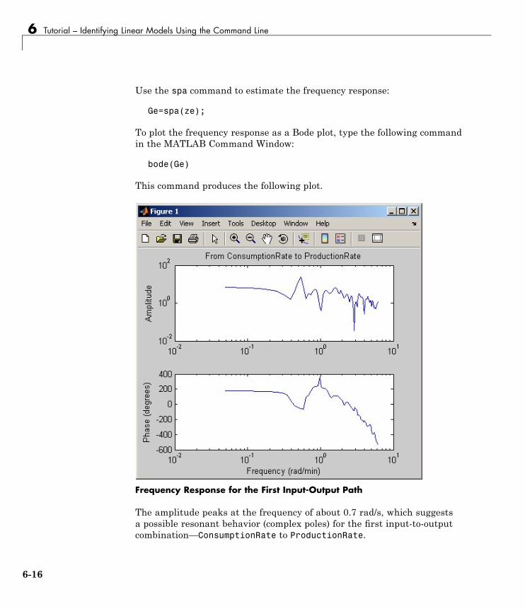
6 Tutorial – Identifying Linear Models Using the Command Line
Use the spa command to estimate the frequency response:
Ge=spa(ze);
To plot the frequency response as a Bode plot, type the following commandin the MATLAB Command Window:
bode(Ge)
This command produces the following plot.
Frequency Response for the First Input-Output Path
The amplitude peaks at the frequency of about 0.7 rad/s, which suggestsa possible resonant behavior (complex poles) for the first input-to-outputcombination—ConsumptionRate to ProductionRate.
6-16
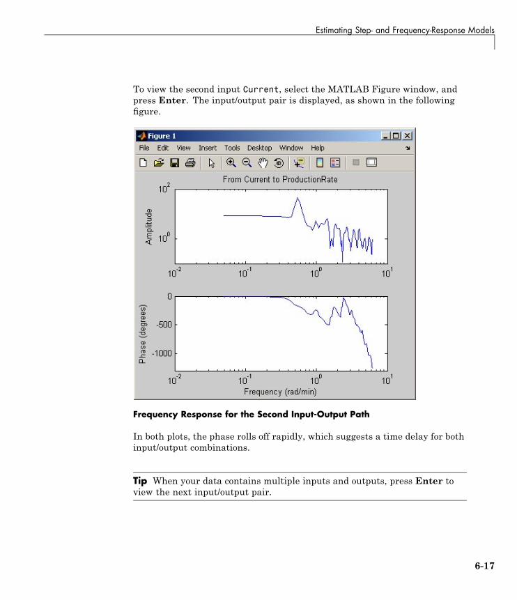
Estimating Step- and Frequency-Response Models
To view the second input Current, select the MATLAB Figure window, andpress Enter. The input/output pair is displayed, as shown in the followingfigure.
Frequency Response for the Second Input-Output Path
In both plots, the phase rolls off rapidly, which suggests a time delay for bothinput/output combinations.
Tip When your data contains multiple inputs and outputs, press Enter toview the next input/output pair.
6-17
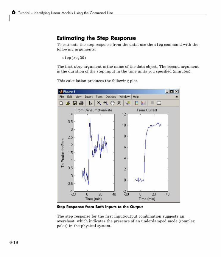
6 Tutorial – Identifying Linear Models Using the Command Line
Estimating the Step ResponseTo estimate the step response from the data, use the step command with thefollowing arguments:
step(ze,30)
The first step argument is the name of the data object. The second argumentis the duration of the step input in the time units you specified (minutes).
This calculation produces the following plot.
Step Response from Both Inputs to the Output
The step response for the first input/output combination suggests anovershoot, which indicates the presence of an underdamped mode (complexpoles) in the physical system.
6-18

Estimating Step- and Frequency-Response Models
The step response from the second input to the output shows no overshoot,which indicates either a first-order response or a higher-order response withreal poles (overdamped response).
The step-response plot indicates a nonzero delay in the system, which isconsistent with the rapid phase roll-off you got in the Bode plot you createdin “Estimating the Step Response” on page 6-18.
6-19
6 Tutorial – Identifying Linear Models Using the Command Line
Estimating Delays in the Multiple-Input System
In this section...
“Why Estimate Delays?” on page 6-20“Estimating Delays Using the ARX Model Structure” on page 6-20“Estimating Delays Using Alternative Methods” on page 6-21
Why Estimate Delays?To identify parametric black-box models, you must specify the input/outputdelay as part of the model order.
If you do not know the input/output delays for your system from theexperiment, you can use the System Identification Toolbox software toestimate the delay.
Estimating Delays Using the ARX Model StructureIn the case of single-input systems, you can read the delay on theimpulse-response plot. However, in the case of multiple-input systems, suchas the one in this tutorial, you might be unable to tell which input caused theinitial change in the output and you can use the delayest command instead.
The delayest command estimates the time delay in a dynamic system byestimating a low-order, discrete-time ARX model with a range of delays, andthen choosing the delay that corresponding to the best fit.
6-20
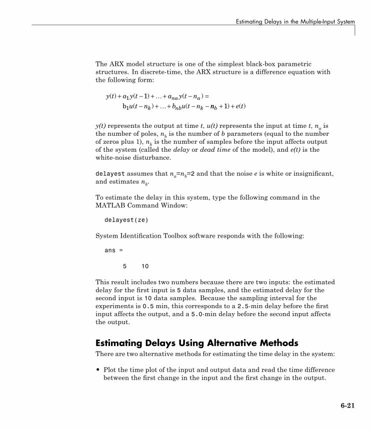
Estimating Delays in the Multiple-Input System
The ARX model structure is one of the simplest black-box parametricstructures. In discrete-time, the ARX structure is a difference equation withthe following form:
y t a y t a y t n
u t n b u t nna a
k nb k
( ) ( ) ( )( ) (
+ − + + − =− + + − −
1 1 …… b1 nn e tb + +1) ( )
y(t) represents the output at time t, u(t) represents the input at time t, na isthe number of poles, nb is the number of b parameters (equal to the numberof zeros plus 1), nk is the number of samples before the input affects outputof the system (called the delay or dead time of the model), and e(t) is thewhite-noise disturbance.
delayest assumes that na=nb=2 and that the noise e is white or insignificant,and estimates nk.
To estimate the delay in this system, type the following command in theMATLAB Command Window:
delayest(ze)
System Identification Toolbox software responds with the following:
ans =
5 10
This result includes two numbers because there are two inputs: the estimateddelay for the first input is 5 data samples, and the estimated delay for thesecond input is 10 data samples. Because the sampling interval for theexperiments is 0.5 min, this corresponds to a 2.5-min delay before the firstinput affects the output, and a 5.0-min delay before the second input affectsthe output.
Estimating Delays Using Alternative MethodsThere are two alternative methods for estimating the time delay in the system:
• Plot the time plot of the input and output data and read the time differencebetween the first change in the input and the first change in the output.
6-21
6 Tutorial – Identifying Linear Models Using the Command Line
This method is practical only for single-input/single-output system; in thecase of multiple-input systems, you might be unable to tell which inputcaused the initial change in the output.
• Plot the impulse response of the data with a 1-standard-deviationconfidence region. You can estimate the time delay using the time whenthe impulse response is first outside the confidence region.
6-22
Estimating Model Orders Using an ARX Model Structure
Estimating Model Orders Using an ARX Model Structure
In this section...
“Why Estimate Model Order?” on page 6-23“Commands for Estimating the Model Order” on page 6-23“Model Order for the First Input-Output Combination” on page 6-25“Model Order for the Second Input-Output Combination” on page 6-28
Why Estimate Model Order?Model order is one or more integers that define the complexity of the model.In general, model order is related to the number of poles, the number of zeros,and the response delay (time in terms of the number of samples before theoutput responds to the input). The specific meaning of model order dependson the model structure.
To compute parametric black-box models, you must provide the model orderas an input. If you do not know the order of your system, you can estimate it.
After completing the steps in this section, you get the following results:
• For the first input/output combination: na=2, nb=2, and the delay nk=5.
• For the second input/output combination: na=1, nb=1, and the delay nk=10.
Later, you explore different model structures by specifying model-order valuesthat are slight variations around these initial estimate.
Commands for Estimating the Model OrderIn this portion of the tutorial, you use struc, arxstruc, and selstruc toestimate and compare simple polynomial (ARX) models for a range of modelorders and delays, and select the best orders based on the quality of the model.
The following list describes the results of using each command:
• struc creates a matrix of model-order combinations for a specified range ofna, nb, and nk values.
6-23
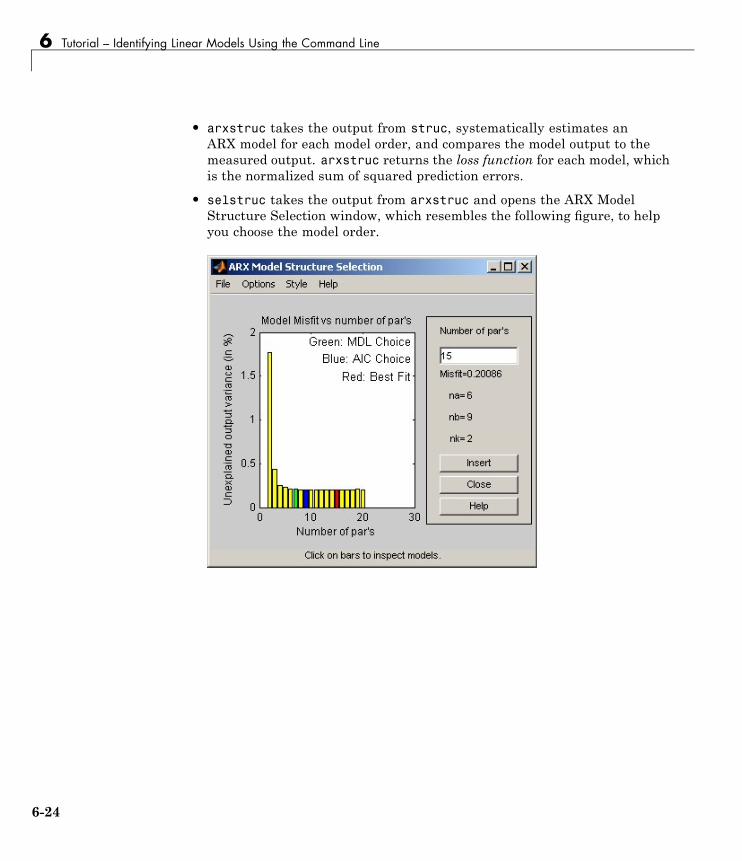
6 Tutorial – Identifying Linear Models Using the Command Line
• arxstruc takes the output from struc, systematically estimates anARX model for each model order, and compares the model output to themeasured output. arxstruc returns the loss function for each model, whichis the normalized sum of squared prediction errors.
• selstruc takes the output from arxstruc and opens the ARX ModelStructure Selection window, which resembles the following figure, to helpyou choose the model order.
6-24
Estimating Model Orders Using an ARX Model Structure
You use the preceding plot to select the best-fit model. The horizontal axisis the total number of parameters:
Number of parameters = +n na b
For the ARX model, na is the number of poles, nb is the number of bparameters (equal to the number of zeros plus 1), and nk is the delay.
The vertical axis, called Unexplained output variance (in %), isthe portion of the output not explained by the model—the ARX modelprediction error for the number of parameters shown on the horizontal axis.The prediction error is the sum of the squares of the differences betweenthe validation data output and the model one-step-ahead predicted output.
Three rectangles are highlighted on the plot in green, blue, and red. Eachcolor indicates a type of best-fit criterion, as follows:
- Red — Best fit minimizes the sum of the squares of the differencebetween the validation data output and the model output. This rectangleindicates the overall best fit.
- Green — Best fit minimizes Rissanen MDL criterion.
- Blue — Best fit minimizes Akaike AIC criterion.
In this tutorial, the Unexplained output variance (in %) value remainsapproximately constant for the combined number of parameters from 4 to20. Such constancy indicates that model performance does not improve athigher orders. Thus, low-order models might fit the data equally well.
Note When you use the same data set for estimation and validation, usethe MDL and AIC criteria to select model orders. These criteria compensatefor overfitting that results from using too many parameters. For moreinformation about these criteria, see the selstruc reference page.
Model Order for the First Input-Output CombinationIn this tutorial, there are two inputs to the system and one output and youestimate model orders for each input/output combination independently. Youcan either estimate the delays from the two inputs simultaneously or oneinput at a time.
6-25
6 Tutorial – Identifying Linear Models Using the Command Line
It makes sense to try the following order combinations for the firstinput/output combination:
• na=2:5
• nb=1:5
• nk=5
This is because the nonparametric models you estimated in “Estimating Step-and Frequency-Response Models” on page 6-15 show that the response for thefirst input/output combination might have a second-order response. Similarly,in “Estimating Delays in the Multiple-Input System” on page 6-20, the delayfor this input/output combination was estimated to be 5.
To estimate model order for the first input/output combination:
1 Use struc to create a matrix of possible model orders.
NN1 = struc(2:5,1:5,5);
2 Use selstruc to compute the loss functions for the ARX models with theorders in NN1.
selstruc(arxstruc(ze(:,:,1),zv(:,:,1),NN1))
Note (ze(:,:,1) selects the first input in the data.
6-26
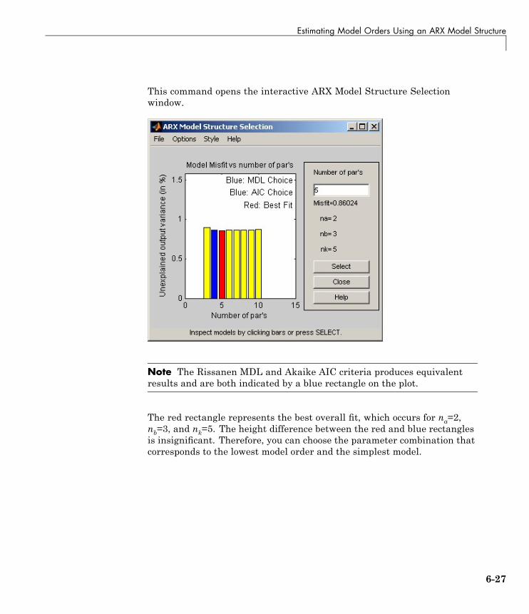
Estimating Model Orders Using an ARX Model Structure
This command opens the interactive ARX Model Structure Selectionwindow.
Note The Rissanen MDL and Akaike AIC criteria produces equivalentresults and are both indicated by a blue rectangle on the plot.
The red rectangle represents the best overall fit, which occurs for na=2,nb=3, and nk=5. The height difference between the red and blue rectanglesis insignificant. Therefore, you can choose the parameter combination thatcorresponds to the lowest model order and the simplest model.
6-27
6 Tutorial – Identifying Linear Models Using the Command Line
3 Click the blue rectangle, and then click Select to choose that combinationof orders:
na=2
nb=2
nk=5
4 To continue, press any key while in the MATLAB Command Window.
Model Order for the Second Input-OutputCombinationIt makes sense to try the following order combinations for the secondinput/output combination:
• na=1:3
• nb=1:3
• nk=10
This is because the nonparametric models you estimated in “Estimating Step-and Frequency-Response Models” on page 6-15 show that the response for thesecond input/output combination might have a first-order response. Similarly,in “Estimating Delays in the Multiple-Input System” on page 6-20, the delayfor this input/output combination was estimated to be 10.
To estimate model order for the second input/output combination:
1 Use struc to create a matrix of possible model orders.
NN2 = struc(1:3,1:3,10);
6-28
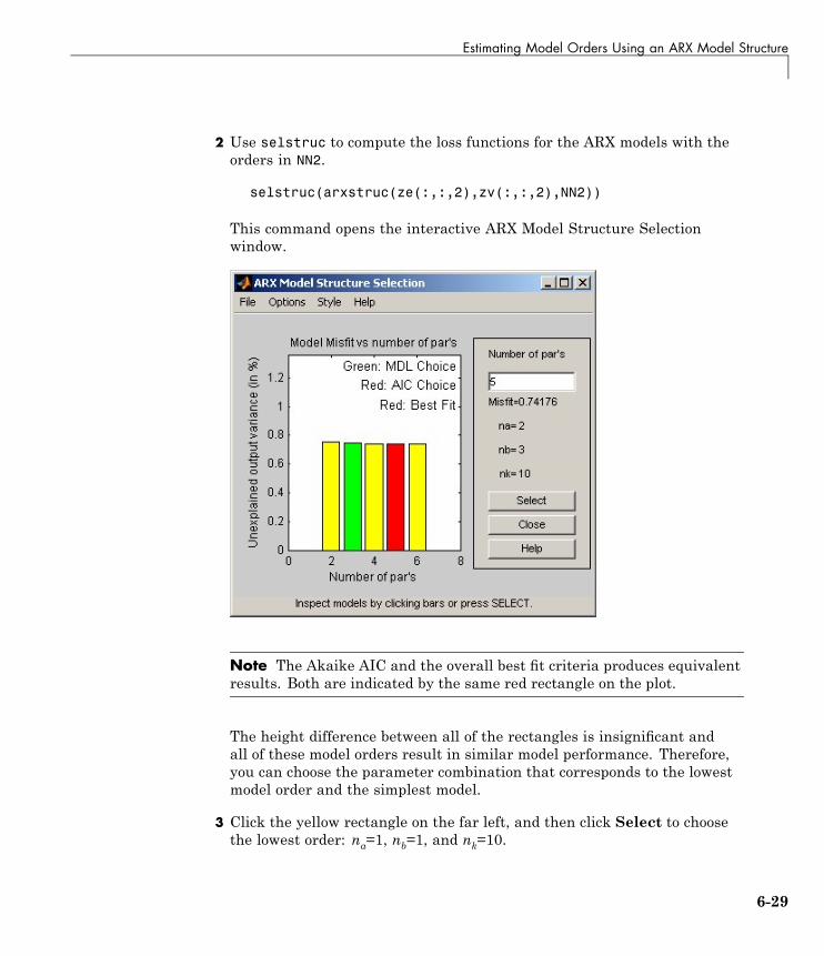
Estimating Model Orders Using an ARX Model Structure
2 Use selstruc to compute the loss functions for the ARX models with theorders in NN2.
selstruc(arxstruc(ze(:,:,2),zv(:,:,2),NN2))
This command opens the interactive ARX Model Structure Selectionwindow.
Note The Akaike AIC and the overall best fit criteria produces equivalentresults. Both are indicated by the same red rectangle on the plot.
The height difference between all of the rectangles is insignificant andall of these model orders result in similar model performance. Therefore,you can choose the parameter combination that corresponds to the lowestmodel order and the simplest model.
3 Click the yellow rectangle on the far left, and then click Select to choosethe lowest order: na=1, nb=1, and nk=10.
6-29
6 Tutorial – Identifying Linear Models Using the Command Line
4 To continue, press any key while in the MATLAB Command Window.
6-30
Estimating Continuous-Time Transfer Functions (Process Models)
Estimating Continuous-Time Transfer Functions (ProcessModels)
In this section...
“Specifying the Structure of the Process Model” on page 6-31“Viewing the Model Structure and Parameter Values” on page 6-32“Specifying Initial Guesses for Time Delays” on page 6-34“Estimating Model Parameters Using pem” on page 6-34“Validating the Process Model” on page 6-36“Estimating a Transfer Function with a Noise Model” on page 6-39
Specifying the Structure of the Process ModelIn this portion of the tutorial, you estimate a low-order, continuous-timetransfer function (process model). the System Identification Toolbox productsupports continuous-time models with at most three poles (which mightcontain underdamped poles), one zero, a delay element, and an integrator.
You must have already prepared your data, as described in “Preparing Data”on page 6-4.
You can use the following results of estimated model orders to specify theorders of the model:
• For the first input/output combination, use:
- Two poles, corresponding to na=2 in the ARX model.
- Delay of 5, corresponding to nk=5 samples (or 2.5 minutes) in the ARXmodel.
• For the second input/output combination, use:
- One pole, corresponding to na=1 in the ARX model.
- Delay of 10, corresponding to nk=10 samples (or 5 minutes) in the ARXmodel.
6-31
6 Tutorial – Identifying Linear Models Using the Command Line
Note Because there is no relationship between the number of zeros estimatedby the discrete-time ARX model and its continuous-time counterpart, youdo not have an estimate for the number of zeros. In this tutorial, you canspecify one zero for the first input/output combination, and no zero for thesecond-output combination.
Use the idproc command to create two model structures, one for eachinput/output combination:
midproc0 = idproc({'P2ZUD','P1D'});
The argument of idproc is a cell array that contains two strings, where eachstring specifies the model structure for each input/output combination:
• 'P2ZUD' represents a transfer function with two poles (P2), one zero (Z),underdamped (complex-conjugate) poles (U) and a delay (D).
• 'P1D' represents a transfer function with one pole (P1) and a delay (D).
Viewing the Model Structure and Parameter ValuesTo view the two resulting models, type the following command in theMATLAB Command Window:
midproc0
6-32
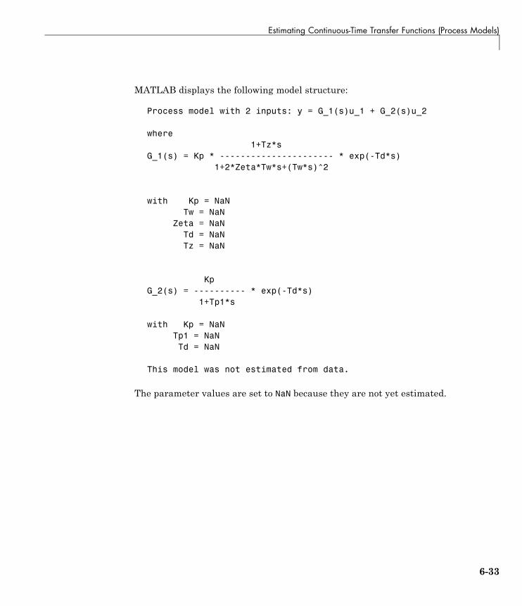
Estimating Continuous-Time Transfer Functions (Process Models)
MATLAB displays the following model structure:
Process model with 2 inputs: y = G_1(s)u_1 + G_2(s)u_2
where1+Tz*s
G_1(s) = Kp * ---------------------- * exp(-Td*s)1+2*Zeta*Tw*s+(Tw*s)^2
with Kp = NaNTw = NaN
Zeta = NaNTd = NaNTz = NaN
KpG_2(s) = ---------- * exp(-Td*s)
1+Tp1*s
with Kp = NaNTp1 = NaNTd = NaN
This model was not estimated from data.
The parameter values are set to NaN because they are not yet estimated.
6-33
6 Tutorial – Identifying Linear Models Using the Command Line
Specifying Initial Guesses for Time DelaysSet the time delay property of the model object to 2.5 min and 5 min for eachinput/output pair as initial guesses. Also, set an upper limit on the delaybecause good initial guesses are available.
midproc0.Td.Value = [2.5 5];midproc0.Td.Max = [3 7];
Note When setting the Td model property, you must specify the delays interms of actual time units (minutes, in this case) and not the number ofsamples.
Estimating Model Parameters Using pempem is an iterative estimation command, which means that it uses an iterativenonlinear least-squares algorithm to minimize a cost function. The costfunction is the weighted sum of the squares of the errors.
Depending on its arguments, pem estimates different black-box polynomialmodels. You can use pem, for example, to estimate parameters for linearcontinuous-time transfer-function, state-space, or polynomial modelstructures. To use pem, you must provide a model structure with unknownparameters and the estimation data as input arguments.
For this portion of the tutorial, you must have already defined the modelstructure, as described in “Specifying the Structure of the Process Model” onpage 6-31. Use midproc0 as the model structure and Ze1 as the estimationdata:
midproc = pem(Ze1,midproc0);present(midproc)
6-34
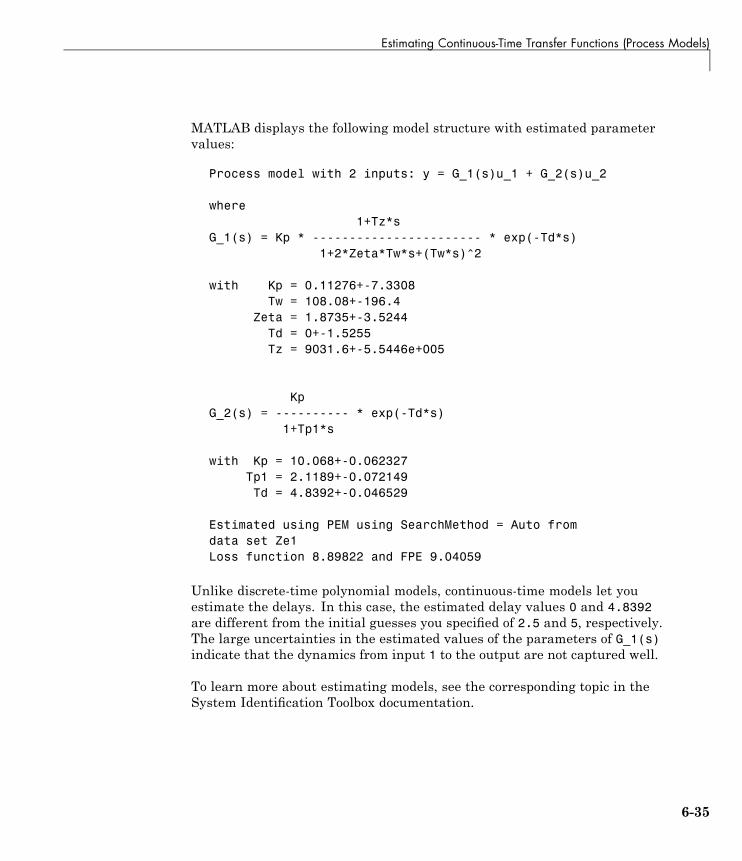
Estimating Continuous-Time Transfer Functions (Process Models)
MATLAB displays the following model structure with estimated parametervalues:
Process model with 2 inputs: y = G_1(s)u_1 + G_2(s)u_2
where1+Tz*s
G_1(s) = Kp * ----------------------- * exp(-Td*s)1+2*Zeta*Tw*s+(Tw*s)^2
with Kp = 0.11276+-7.3308Tw = 108.08+-196.4
Zeta = 1.8735+-3.5244Td = 0+-1.5255Tz = 9031.6+-5.5446e+005
KpG_2(s) = ---------- * exp(-Td*s)
1+Tp1*s
with Kp = 10.068+-0.062327Tp1 = 2.1189+-0.072149Td = 4.8392+-0.046529
Estimated using PEM using SearchMethod = Auto fromdata set Ze1Loss function 8.89822 and FPE 9.04059
Unlike discrete-time polynomial models, continuous-time models let youestimate the delays. In this case, the estimated delay values 0 and 4.8392are different from the initial guesses you specified of 2.5 and 5, respectively.The large uncertainties in the estimated values of the parameters of G_1(s)indicate that the dynamics from input 1 to the output are not captured well.
To learn more about estimating models, see the corresponding topic in theSystem Identification Toolbox documentation.
6-35
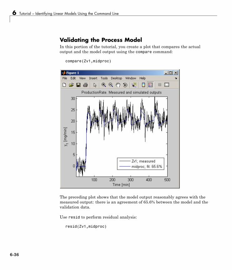
6 Tutorial – Identifying Linear Models Using the Command Line
Validating the Process ModelIn this portion of the tutorial, you create a plot that compares the actualoutput and the model output using the compare command:
compare(Zv1,midproc)
The preceding plot shows that the model output reasonably agrees with themeasured output: there is an agreement of 65.6% between the model and thevalidation data.
Use resid to perform residual analysis:
resid(Zv1,midproc)
6-36
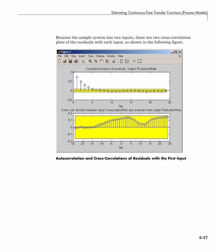
Estimating Continuous-Time Transfer Functions (Process Models)
Because the sample system has two inputs, there are two cross-correlationplots of the residuals with each input, as shown in the following figure.
Autocorrelation and Cross-Correlations of Residuals with the First Input
6-37
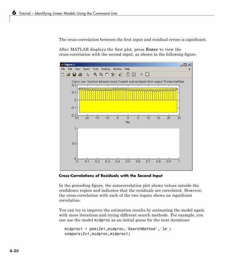
6 Tutorial – Identifying Linear Models Using the Command Line
The cross-correlation between the first input and residual errors is significant.
After MATLAB displays the first plot, press Enter to view thecross-correlation with the second input, as shown in the following figure.
Cross-Correlations of Residuals with the Second Input
In the preceding figure, the autocorrelation plot shows values outside theconfidence region and indicates that the residuals are correlated. However,the cross-correlation with each of the two inputs shows no significantcorrelation.
You can try to improve the estimation results by estimating the model againwith more iterations and trying different search methods. For example, youcan use the model midproc as an initial guess for the next iterations:
midproc1 = pem(Ze1,midproc,'SearchMethod','lm')compare(Zv1,midproc,midproc1)
6-38
Estimating Continuous-Time Transfer Functions (Process Models)
resid(Zv1, midproc1)
The resulting plots show an improved fit of the simulated model outputto the validation data and a reduced correlation in the residuals. TheSearchMethod='lm' setting uses the Levenberg-Marquardt method foriterative parameter estimation.
For more information about the SearchMethod field of the Algorithm modelproperty of linear models, see the corresponding reference page.
Estimating a Transfer Function with a Noise ModelThis portion of the tutorial shows how to estimate a process model and includea noise model in the estimation. Including a noise model typically improvesmodel prediction results but not necessarily the simulation results.
Use the following command to specify a first-order ARMA noise:
midproc2 = pem(Ze1,midproc0,'DisturbanceModel','arma1')
Note You can type 'dist' instead of 'DisturbanceModel'. Property namesare not case sensitive, and you only need to include the portion of the namethat uniquely identifies the property.
Compare the resulting model to the measured data and perform residualanalysis, as follows:
compare(Zv1,midproc2)figureresid(Zv1,midproc2)
6-39
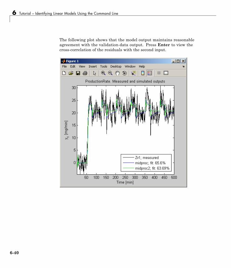
6 Tutorial – Identifying Linear Models Using the Command Line
The following plot shows that the model output maintains reasonableagreement with the validation-data output. Press Enter to view thecross-correlation of the residuals with the second input.
6-40
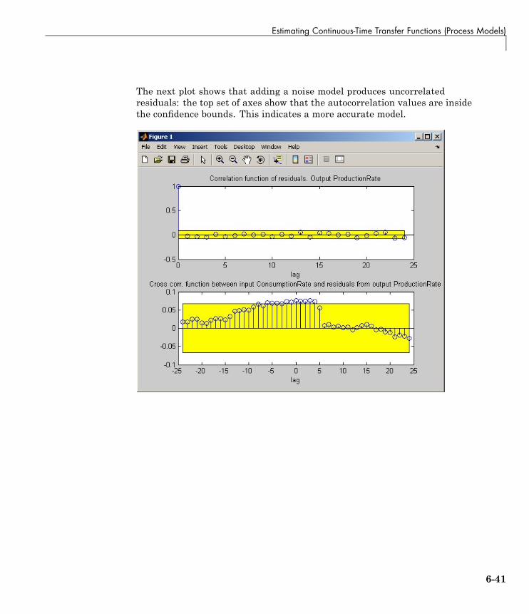
Estimating Continuous-Time Transfer Functions (Process Models)
The next plot shows that adding a noise model produces uncorrelatedresiduals: the top set of axes show that the autocorrelation values are insidethe confidence bounds. This indicates a more accurate model.
6-41
6 Tutorial – Identifying Linear Models Using the Command Line
Estimating Black-Box Polynomial Models
In this section...
“Model Orders for Estimating Polynomial Models” on page 6-42“Estimating a Linear ARX Model” on page 6-43“Estimating a State-Space Model” on page 6-46“Estimating a Box-Jenkins Model” on page 6-49“Comparing Model Output to Measured Output” on page 6-51
Model Orders for Estimating Polynomial ModelsIn this portion of the tutorial, you estimate several different types ofblack-box, input-output polynomial models.
You must have already prepared your data, as described in “Preparing Data”on page 6-4.
You can use the following previous results of estimated model orders to specifythe orders of the polynomial model:
• For the first input/output combination, use:
- Two poles, corresponding to na=2 in the ARX model.
- One zero, corresponding to nb=2 in the ARX model.
- Delay of 5, corresponding to nk=5 samples (or 2.5 minutes) in the ARXmodel.
• For the second input/output combination, use:
- One pole, corresponding to na=1 in the ARX model.
- No zeros, corresponding to nb=1 in the ARX model.
- Delay of 10, corresponding to nk=10 samples (or 5 minutes) in the ARXmodel.
6-42
Estimating Black-Box Polynomial Models
Estimating a Linear ARX Model
• “About ARX Models” on page 6-43
• “Estimating ARX Models Using arx” on page 6-43
• “Accessing Model Data” on page 6-45
• “Learn More” on page 6-46
About ARX ModelsFor a single-input/single-output system (SISO), the ARX model structure is:
y t a y t a y t n
u t n b u t nna a
k nb k
( ) ( ) ( )( ) (
+ − + + − =− + + − −
1 1 …… b1 nn e tb + +1) ( )
y(t) represents the output at time t, u(t) represents the input at time t, na isthe number of poles, nb is the number of zeros plus 1, nk is the number ofsamples before the input affects output of the system (called the delay or deadtime of the model), and e(t) is the white-noise disturbance.
The ARX model structure does not distinguish between the poles forindividual input/output paths: dividing the ARX equation by A, whichcontains the poles, shows that A appears in the denominator for both inputs.Therefore, you can set na to the sum of the poles for each input/output pair,which is equal to 3 in this case.
The System Identification Toolbox product estimates the parameters a an1 …
and b bn1 … using the data and the model orders you specify.
Estimating ARX Models Using arxUse arx to compute the polynomial coefficients using the fast, noniterativemethod arx:
marx = arx(Ze1,'na',3,'nb',[2 1],'nk',[5 10]);present(marx) % Displays model parameters
% with uncertainty information
6-43
6 Tutorial – Identifying Linear Models Using the Command Line
MATLAB estimates the polynomials A, B1, and B2:
Discrete-time IDPOLY model: A(q)y(t) = B(q)u(t) + e(t)A(q) = 1 - 1.027 (+-0.02917) q^-1
+ 0.1675 (+-0.04214) q^-2+ 0.01307 (+-0.02591) q^-3
B1(q) = 1.86 (+-0.1896) q^-5 - 1.608 (+-0.1894) q^-6B2(q) = 1.612 (+-0.07417) q^-10
The uncertainty for each of the model parameters is computed to 1 standarddeviation and appears in parentheses next to each parameter value.
Tip Alternatively, you can use the following shorthand syntax and specifymodel orders as a single vector:
marx = arx(Ze1,[3 2 1 5 10])
6-44
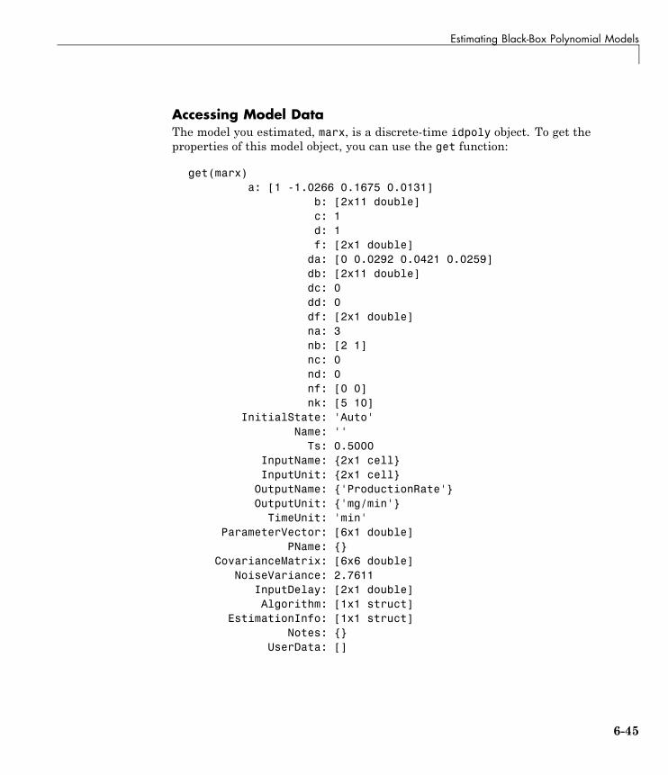
Estimating Black-Box Polynomial Models
Accessing Model DataThe model you estimated, marx, is a discrete-time idpoly object. To get theproperties of this model object, you can use the get function:
get(marx)a: [1 -1.0266 0.1675 0.0131]
b: [2x11 double]c: 1d: 1f: [2x1 double]
da: [0 0.0292 0.0421 0.0259]db: [2x11 double]dc: 0dd: 0df: [2x1 double]na: 3nb: [2 1]nc: 0nd: 0nf: [0 0]nk: [5 10]
InitialState: 'Auto'Name: ''
Ts: 0.5000InputName: {2x1 cell}InputUnit: {2x1 cell}
OutputName: {'ProductionRate'}OutputUnit: {'mg/min'}
TimeUnit: 'min'ParameterVector: [6x1 double]
PName: {}CovarianceMatrix: [6x6 double]
NoiseVariance: 2.7611InputDelay: [2x1 double]Algorithm: [1x1 struct]
EstimationInfo: [1x1 struct]Notes: {}
UserData: []
6-45
6 Tutorial – Identifying Linear Models Using the Command Line
You can access the information stored by these properties using dot notation.For example, you can compute the discrete poles of the model by finding theroots of the A polynomial:
marx_poles=roots(marx.a)
marx_poles =
0.79530.2883
-0.0570
In this case, you access the A polynomial using marx.a.
The model marx describes system dynamics using three discrete poles.
Tip You can also use the zpkdata command to compute the poles of a modeldirectly.
Learn MoreTo learn more about estimating polynomial models, see the correspondingsections in the System Identification Toolbox User’s Guide.
For more information about accessing model data, see the topic on extractingnumerical data from linear models in the System Identification Toolbox User’sGuide.
Estimating a State-Space Model
• “About State-Space Models” on page 6-47
• “Estimating State-Space Models Using n4sid” on page 6-47
• “Learn More” on page 6-49
6-46

Estimating Black-Box Polynomial Models
About State-Space ModelsThe general state-space model structure is:
x t Ax t Bu t Ke ty t Cx t Du t e t( ) ( ) ( ) ( )( ) ( ) ( ) ( )
+ = + += + +1
y(t) represents the output at time t, u(t) represents the input at time t, x(t) isthe state vector at time t, and e(t) is the white-noise disturbance.
You must specify a single integer as the model order (dimension of the statevector) to estimate a state-space model. By default, the delay equals 1.
The System Identification Toolbox product estimates the state-space matricesA, B, C, D, and K using the model order and the data you specify.
The state-space model structure is a good choice for quick estimation becauseit contains only two parameters: n is the number of poles (the size of the Amatrix) and nk is the delay.
Estimating State-Space Models Using n4sidUse the n4sid command to specify a range of model orders and evaluate theperformance of several state-space models (orders 2 to 8):
mn4sid = n4sid(Ze1,2:8,'nk',[5 10]);
6-47
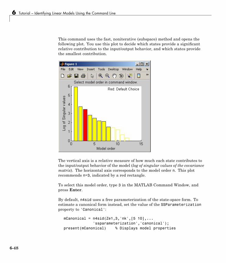
6 Tutorial – Identifying Linear Models Using the Command Line
This command uses the fast, noniterative (subspace) method and opens thefollowing plot. You use this plot to decide which states provide a significantrelative contribution to the input/output behavior, and which states providethe smallest contribution.
The vertical axis is a relative measure of how much each state contributes tothe input/output behavior of the model (log of singular values of the covariancematrix). The horizontal axis corresponds to the model order n. This plotrecommends n=3, indicated by a red rectangle.
To select this model order, type 3 in the MATLAB Command Window, andpress Enter.
By default, n4sid uses a free parameterization of the state-space form. Toestimate a canonical form instead, set the value of the SSParameterizationproperty to 'Canonical':
mCanonical = n4sid(Ze1,3,'nk',[5 10],...'ssparameterization','canonical');
present(mCanonical) % Displays model properties
6-48
Estimating Black-Box Polynomial Models
Note When you examine the displayed properties, notice that the modelorder is high. This high order occurs because the model uses additional statesto incorporate input delays.
Learn MoreTo learn more about estimating state-space models, see the correspondingtopic in the System Identification Toolbox User’s Guide.
Estimating a Box-Jenkins Model
• “About Box-Jenkins Models” on page 6-49
• “Estimating a BJ Model Using pem” on page 6-49
• “Learn More” on page 6-51
About Box-Jenkins ModelsThe general Box-Jenkins (BJ) structure is:
y tB qF q
u t nkC qD q
e ti
ii i
i
nu( )
( )( )
( )( )
( )= −( ) +=∑
1
To estimate a BJ model, you need to specify the parameters nb, nf, nc, nd,and nk.
Whereas the ARX model structure does not distinguish between the polesfor individual input/output paths, the BJ model provides more flexibility inmodeling the poles and zeros of the disturbance separately from the polesand zeros of the system dynamics.
Estimating a BJ Model Using pemYou can use pem to estimate the BJ model. pem is an iterative method and hasthe following general syntax:
pem(data,'na',na,'nb',nb,'nc',nc,'nd',nd,'nf',nf,'nk',nk)
6-49
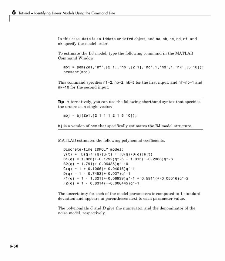
6 Tutorial – Identifying Linear Models Using the Command Line
In this case, data is an iddata or idfrd object, and na, nb, nc, nd, nf, andnk specify the model order.
To estimate the BJ model, type the following command in the MATLABCommand Window:
mbj = pem(Ze1,'nf',[2 1],'nb',[2 1],'nc',1,'nd',1,'nk',[5 10]);present(mbj)
This command specifies nf=2, nb=2, nk=5 for the first input, and nf=nb=1 andnk=10 for the second input.
Tip Alternatively, you can use the following shorthand syntax that specifiesthe orders as a single vector:
mbj = bj(Ze1,[2 1 1 1 2 1 5 10]);
bj is a version of pem that specifically estimates the BJ model structure.
MATLAB estimates the following polynomial coefficients:
Discrete-time IDPOLY model:y(t) = [B(q)/F(q)]u(t) + [C(q)/D(q)]e(t)B1(q) = 1.823(+-0.1792)q^-5 - 1.315(+-0.2368)q^-6B2(q) = 1.791(+-0.06435)q^-10C(q) = 1 + 0.1066(+-0.04015)q^-1D(q) = 1 - 0.7453(+-0.027)q^-1F1(q) = 1 - 1.321(+-0.06939)q^-1 + 0.5911(+-0.05516)q^-2F2(q) = 1 - 0.8314(+-0.006445)q^-1
The uncertainty for each of the model parameters is computed to 1 standarddeviation and appears in parentheses next to each parameter value.
The polynomials C and D give the numerator and the denominator of thenoise model, respectively.
6-50
Estimating Black-Box Polynomial Models
Learn MoreTo learn more about estimating BJ models, see the corresponding topic in theSystem Identification Toolbox User’s Guide.
Comparing Model Output to Measured OutputTo compare the output of the ARX, state-space, and Box-Jenkins models tothe measured output, use the compare function:
compare(Zv1,marx,mn4sid,mbj)
compare plots the measured output in the validation data set against thesimulated output from the models. The input data from the validation dataset serves as input to the models.
6-51
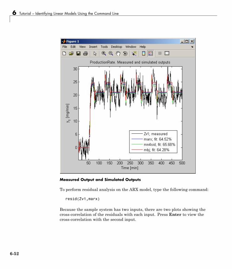
6 Tutorial – Identifying Linear Models Using the Command Line
Measured Output and Simulated Outputs
To perform residual analysis on the ARX model, type the following command:
resid(Zv1,marx)
Because the sample system has two inputs, there are two plots showing thecross-correlation of the residuals with each input. Press Enter to view thecross-correlation with the second input.
6-52
Estimating Black-Box Polynomial Models
To perform residual analysis on the state-space model, type the followingcommand:
resid(Zv1,mn4sid)
Finally, to perform residual analysis on the BJ model, type the followingcommand:
resid(Zv1,mbj)
All three models simulate the output equally well and have uncorrelatedresiduals. Therefore, choose the ARX model because it is the simplest of thethree input-output polynomial models and adequately captures the processdynamics.
6-53
6 Tutorial – Identifying Linear Models Using the Command Line
Simulating and Predicting Model Output
In this section...
“Simulating the Model Output” on page 6-54“Predicting the Future Output” on page 6-55
Simulating the Model OutputIn this portion of the tutorial, you simulate the model output. You musthave already created the continuous-time model midproc2, as described in“Estimating Continuous-Time Transfer Functions (Process Models)” on page6-31.
Simulating the model output requires the following information:
• Input values to the model
• Initial conditions for the simulation (also called initial states)
For example, the following commands use the iddata and idinput commandsto construct an input data set, and use sim to simulate the model output:
% Create input for simulationU = iddata([],idinput([200 2]),'Ts',0.5);% Simulate the response setting initial conditions% equal to zeroysim_1 = sim(midproc2,U,'InitialState','zero')
To match the simulated response of a model to the measured output for thesame input, compute the initial states corresponding to the measured data.You can ensure that the simulated response of the model midproc2 providesa good fit to the measured data Zv1 by using findstates(idmodel). Thefollowing command estimates the initial states X0est from the data set Zv1:
X0est = findstates(midproc2,Zv1);
Next, simulate the model using the initial states estimated from the data:
Usim = Zv1.u; % Simulation inputysim_2 = sim(midproc2,Usim,'InitialState',X0est);
6-54
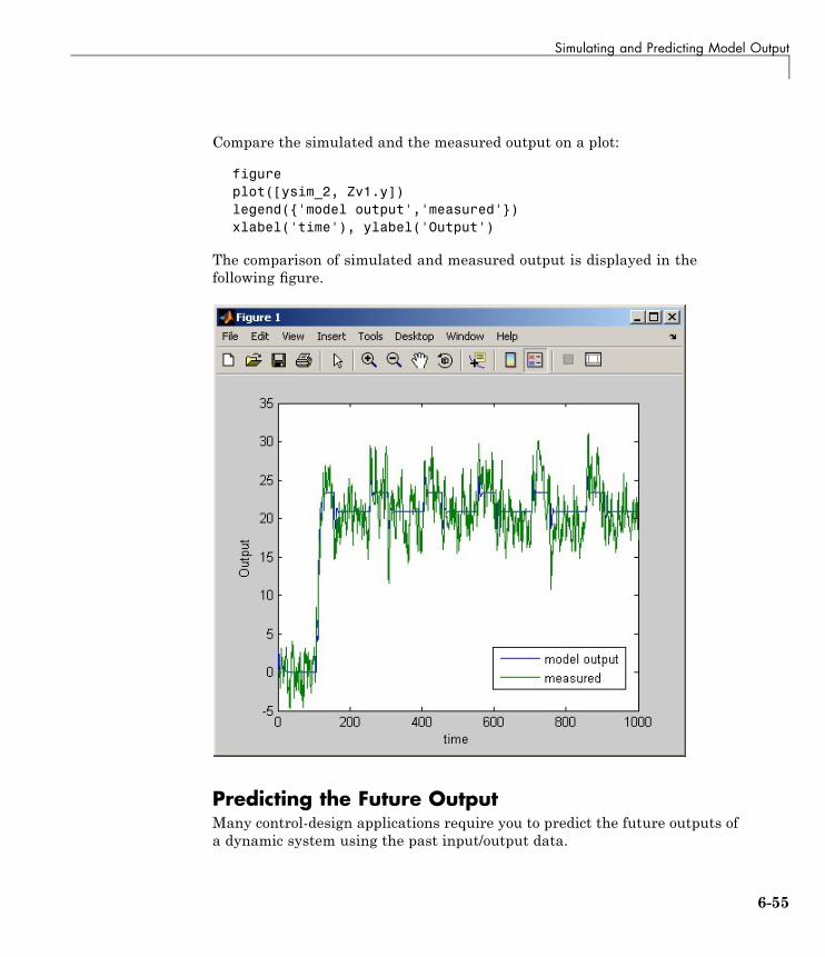
Simulating and Predicting Model Output
Compare the simulated and the measured output on a plot:
figureplot([ysim_2, Zv1.y])legend({'model output','measured'})xlabel('time'), ylabel('Output')
The comparison of simulated and measured output is displayed in thefollowing figure.
Predicting the Future OutputMany control-design applications require you to predict the future outputs ofa dynamic system using the past input/output data.
6-55
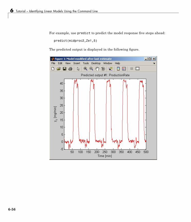
6 Tutorial – Identifying Linear Models Using the Command Line
For example, use predict to predict the model response five steps ahead:
predict(midproc2,Ze1,5)
The predicted output is displayed in the following figure.
6-56
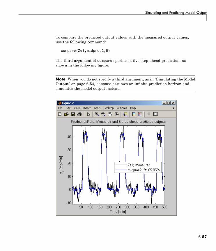
Simulating and Predicting Model Output
To compare the predicted output values with the measured output values,use the following command:
compare(Ze1,midproc2,5)
The third argument of compare specifies a five-step-ahead prediction, asshown in the following figure.
Note When you do not specify a third argument, as in “Simulating the ModelOutput” on page 6-54, compare assumes an infinite prediction horizon andsimulates the model output instead.
6-57
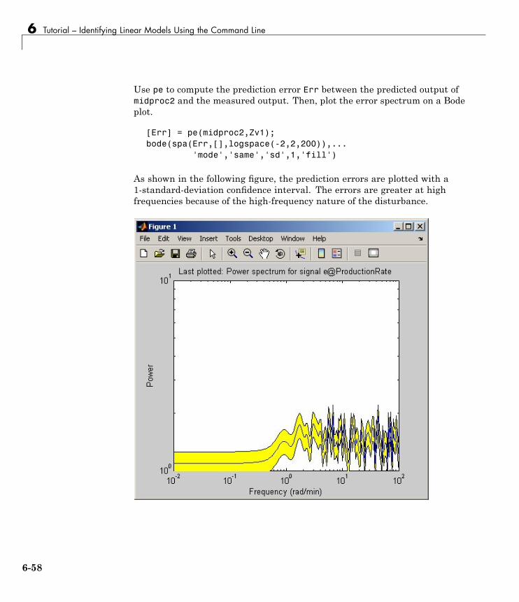
6 Tutorial – Identifying Linear Models Using the Command Line
Use pe to compute the prediction error Err between the predicted output ofmidproc2 and the measured output. Then, plot the error spectrum on a Bodeplot.
[Err] = pe(midproc2,Zv1);bode(spa(Err,[],logspace(-2,2,200)),...
'mode','same','sd',1,'fill')
As shown in the following figure, the prediction errors are plotted with a1-standard-deviation confidence interval. The errors are greater at highfrequencies because of the high-frequency nature of the disturbance.
6-58
7
Tutorial – IdentifyingNonlinear Black-BoxModels Using the GUI
• “About This Tutorial” on page 7-2
• “Preparing Data” on page 7-4
• “Estimating Nonlinear ARX Models” on page 7-9
• “Estimating Hammerstein-Wiener Models” on page 7-22
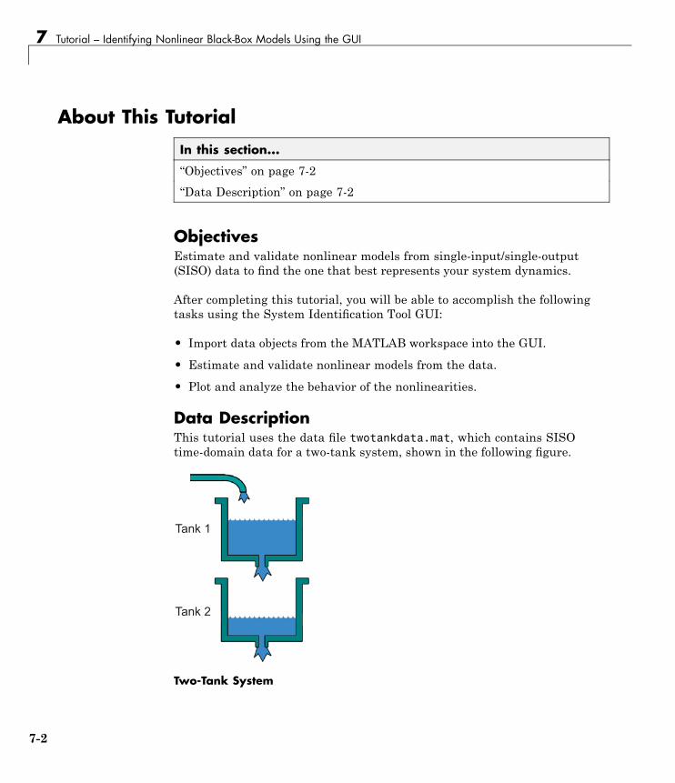
7 Tutorial – Identifying Nonlinear Black-Box Models Using the GUI
About This Tutorial
In this section...
“Objectives” on page 7-2“Data Description” on page 7-2
ObjectivesEstimate and validate nonlinear models from single-input/single-output(SISO) data to find the one that best represents your system dynamics.
After completing this tutorial, you will be able to accomplish the followingtasks using the System Identification Tool GUI:
• Import data objects from the MATLAB workspace into the GUI.
• Estimate and validate nonlinear models from the data.
• Plot and analyze the behavior of the nonlinearities.
Data DescriptionThis tutorial uses the data file twotankdata.mat, which contains SISOtime-domain data for a two-tank system, shown in the following figure.
������
������
Two-Tank System
7-2
About This Tutorial
In the two-tank system, water pours through a pipe into Tank 1, drains intoTank 2, and leaves the system through a small hole at the bottom of Tank2. The measured input u(t) to the system is the voltage applied to the pumpthat feeds the water into Tank 1 (in volts). The measured output y(t) is theheight of the water in the lower tank (in meters).
Based on Bernoulli’s law, which states that water flowing through a smallhole at the bottom of a tank depends nonlinearly on the level of the water inthe tank, you expect the relationship between the input and the output datato be nonlinear.
twotankdata.mat includes 3000 samples with a sampling interval of 0.2 s.
7-3
7 Tutorial – Identifying Nonlinear Black-Box Models Using the GUI
Preparing Data
In this section...
“Loading Data into the MATLAB Workspace” on page 7-4“Creating iddata Objects” on page 7-4“Starting the System Identification Tool” on page 7-6“Importing Data Objects into the System Identification Tool” on page 7-7
Loading Data into the MATLAB WorkspaceLoad sample data in twotankdata.mat by typing the following commandin the MATLAB Command Window:
load twotankdata
This command loads the following two variables into the MATLAB Workspacebrowser:
• y is the output data, which is the water height in Tank 2 (in meters).
• u is the input data, which is the voltage applied to the pump that feeds thewater into Tank 1 (in volts).
Creating iddata ObjectsSystem Identification Toolbox data objects encapsulate both data values anddata properties into a single entity. You can use the System IdentificationToolbox commands to conveniently manipulate these data objects as singleentities.
You must have already loaded the sample data into the MATLAB workspace,as described in “Loading Data into the MATLAB Workspace” on page 7-4.
7-4
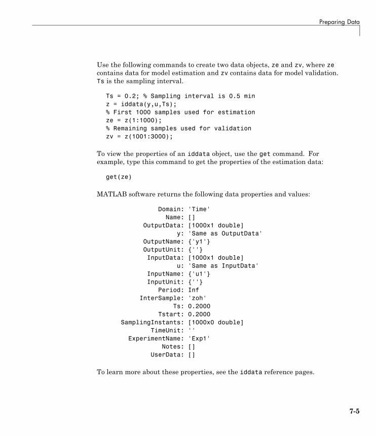
Preparing Data
Use the following commands to create two data objects, ze and zv, where zecontains data for model estimation and zv contains data for model validation.Ts is the sampling interval.
Ts = 0.2; % Sampling interval is 0.5 minz = iddata(y,u,Ts);% First 1000 samples used for estimationze = z(1:1000);% Remaining samples used for validationzv = z(1001:3000);
To view the properties of an iddata object, use the get command. Forexample, type this command to get the properties of the estimation data:
get(ze)
MATLAB software returns the following data properties and values:
Domain: 'Time'Name: []
OutputData: [1000x1 double]y: 'Same as OutputData'
OutputName: {'y1'}OutputUnit: {''}InputData: [1000x1 double]
u: 'Same as InputData'InputName: {'u1'}InputUnit: {''}
Period: InfInterSample: 'zoh'
Ts: 0.2000Tstart: 0.2000
SamplingInstants: [1000x0 double]TimeUnit: ''
ExperimentName: 'Exp1'Notes: []
UserData: []
To learn more about these properties, see the iddata reference pages.
7-5
7 Tutorial – Identifying Nonlinear Black-Box Models Using the GUI
To modify data properties, you can use dot notation or the set command. Forexample, to assign channel names and units that label plot axes, type thefollowing syntax in the MATLAB Command Window:
% Set time units to minutesze.TimeUnit = 'sec';% Set names of input channelsze.InputName = 'Voltage';% Set units for input variablesze.InputUnit = 'V';% Set name of output channelze.OutputName = 'Height';% Set unit of output channelze.OutputUnit = 'm';
% Set validation data propertieszv.TimeUnit = 'sec';zv.InputName = 'Voltage';zv.InputUnit = 'V';zv.OutputName = 'Height';zv.OutputUnit = 'm';
To verify that the InputName property of ze is changed, type the followingcommand:
ze.inputname
Tip Property names, such as InputName, are not case sensitive. You can alsoabbreviate property names that start with Input or Output by substituting ufor Input and y for Output in the property name. For example, OutputUnit isequivalent to yunit.
Starting the System Identification ToolTo open the System Identification Tool GUI, type the following commandin the MATLAB Command Window:
ident
7-6
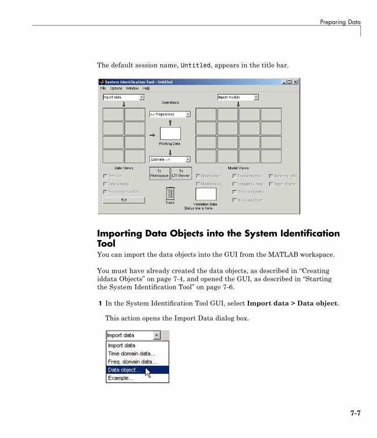
Preparing Data
The default session name, Untitled, appears in the title bar.
Importing Data Objects into the System IdentificationToolYou can import the data objects into the GUI from the MATLAB workspace.
You must have already created the data objects, as described in “Creatingiddata Objects” on page 7-4, and opened the GUI, as described in “Startingthe System Identification Tool” on page 7-6.
1 In the System Identification Tool GUI, select Import data > Data object.
This action opens the Import Data dialog box.
7-7
7 Tutorial – Identifying Nonlinear Black-Box Models Using the GUI
2 Enter ze in the Object field to import the estimation data. Press Enter.
This action enters the object information into the Import Data fields.
Click More to view the following additional information about this data,including channel names and units.
3 Click Import to add the icon named ze to the System Identification ToolGUI.
4 In the Import Data dialog box, type zv in the Object field to import thevalidation data. Press Enter.
5 Click Import to add the icon named zv to the System Identification ToolGUI.
6 In the Import Data dialog box, click Close.
7 In the System Identification Tool GUI, drag the validationg data zv iconto the Validation Data rectangle. The estimation data ze icon is alreadydesignated in the Working Data rectangle.
7-8
Estimating Nonlinear ARX Models
Estimating Nonlinear ARX Models
In this section...
“Estimating a Nonlinear ARX Model with Default Settings” on page 7-9“Plotting Nonlinearity Cross-Sections for Nonlinear ARX Models” on page7-13“Changing the Nonlinear ARX Model Structure” on page 7-16“Selecting a Subset of Regressors in the Nonlinear Block” on page 7-18“Changing the Nonlinearity Estimator in a Nonlinear ARX Model” on page7-20“Selecting the Best Model” on page 7-21
Estimating a Nonlinear ARX Model with DefaultSettingsIn this portion of the tutorial, you estimate a nonlinear ARX model usingdefault model structure and estimation options.
You must have already prepared the data, as described in “Preparing Data”on page 7-4. For more information about nonlinear ARX models, see
7-9
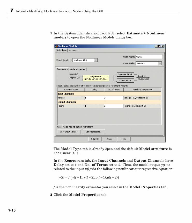
7 Tutorial – Identifying Nonlinear Black-Box Models Using the GUI
1 In the System Identification Tool GUI, select Estimate > Nonlinearmodels to open the Nonlinear Models dialog box.
TheModel Type tab is already open and the default Model structure isNonlinear ARX.
In the Regressors tab, the Input Channels and Output Channels haveDelay set to 1 and No. of Terms set to 2. Thus, the model output y(t) isrelated to the input u(t) via the following nonlinear autoregressive equation:
y t f y t y t u t u t( ) ( ), ( ), ( ), ( )= − − − −( )1 2 1 2
f is the nonlinearity estimator you select in theModel Properties tab.
2 Click the Model Properties tab.
7-10
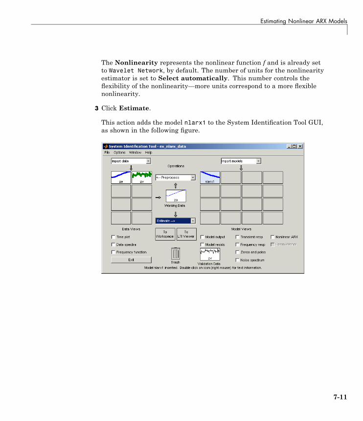
Estimating Nonlinear ARX Models
The Nonlinearity represents the nonlinear function f and is already setto Wavelet Network, by default. The number of units for the nonlinearityestimator is set to Select automatically. This number controls theflexibility of the nonlinearity—more units correspond to a more flexiblenonlinearity.
3 Click Estimate.
This action adds the model nlarx1 to the System Identification Tool GUI,as shown in the following figure.
7-11
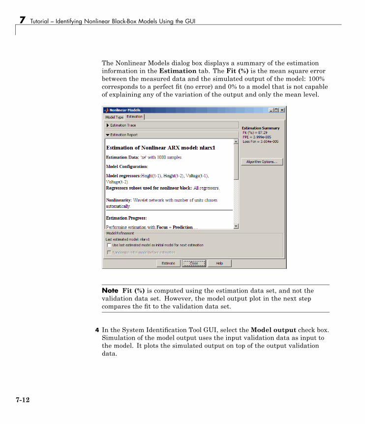
7 Tutorial – Identifying Nonlinear Black-Box Models Using the GUI
The Nonlinear Models dialog box displays a summary of the estimationinformation in the Estimation tab. The Fit (%) is the mean square errorbetween the measured data and the simulated output of the model: 100%corresponds to a perfect fit (no error) and 0% to a model that is not capableof explaining any of the variation of the output and only the mean level.
Note Fit (%) is computed using the estimation data set, and not thevalidation data set. However, the model output plot in the next stepcompares the fit to the validation data set.
4 In the System Identification Tool GUI, select theModel output check box.Simulation of the model output uses the input validation data as input tothe model. It plots the simulated output on top of the output validationdata.
7-12
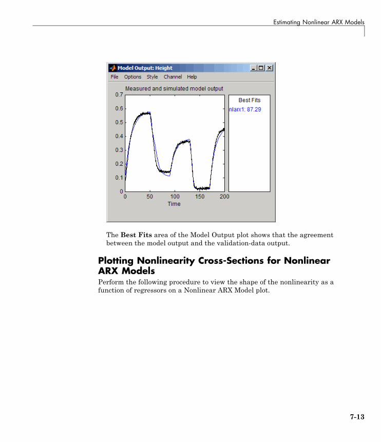
Estimating Nonlinear ARX Models
The Best Fits area of the Model Output plot shows that the agreementbetween the model output and the validation-data output.
Plotting Nonlinearity Cross-Sections for NonlinearARX ModelsPerform the following procedure to view the shape of the nonlinearity as afunction of regressors on a Nonlinear ARX Model plot.
7-13
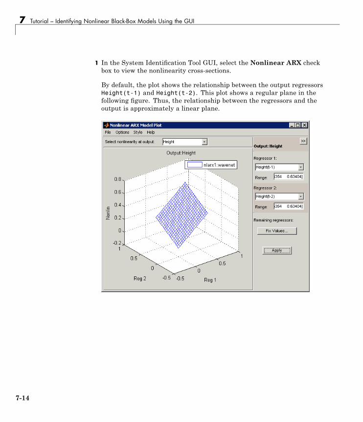
7 Tutorial – Identifying Nonlinear Black-Box Models Using the GUI
1 In the System Identification Tool GUI, select the Nonlinear ARX checkbox to view the nonlinearity cross-sections.
By default, the plot shows the relationship between the output regressorsHeight(t-1) and Height(t-2). This plot shows a regular plane in thefollowing figure. Thus, the relationship between the regressors and theoutput is approximately a linear plane.
7-14

Estimating Nonlinear ARX Models
2 In the Nonlinear ARX Model Plot window, set Regressor 1 toVoltage(t-1). Set Regressor 2 to Voltage(t-2). Click Apply.
The relationship between these regressors and the output is nonlinear, asshown in the following plot.
3 To rotate the nonlinearity surface, select Style > Rotate 3D and dragthe plot to a new orientation.
4 To display a 1-D cross-section for Regressor 1, set Regressor 2 to none,and click Apply. The following figure shows the resulting nonlinearity
7-15
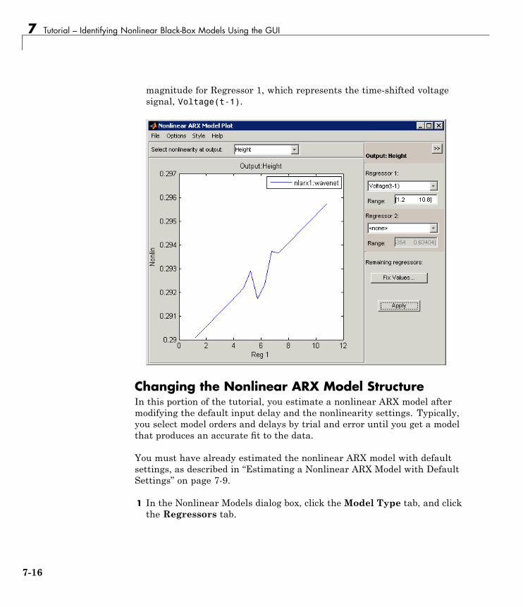
7 Tutorial – Identifying Nonlinear Black-Box Models Using the GUI
magnitude for Regressor 1, which represents the time-shifted voltagesignal, Voltage(t-1).
Changing the Nonlinear ARX Model StructureIn this portion of the tutorial, you estimate a nonlinear ARX model aftermodifying the default input delay and the nonlinearity settings. Typically,you select model orders and delays by trial and error until you get a modelthat produces an accurate fit to the data.
You must have already estimated the nonlinear ARX model with defaultsettings, as described in “Estimating a Nonlinear ARX Model with DefaultSettings” on page 7-9.
1 In the Nonlinear Models dialog box, click the Model Type tab, and clickthe Regressors tab.
7-16
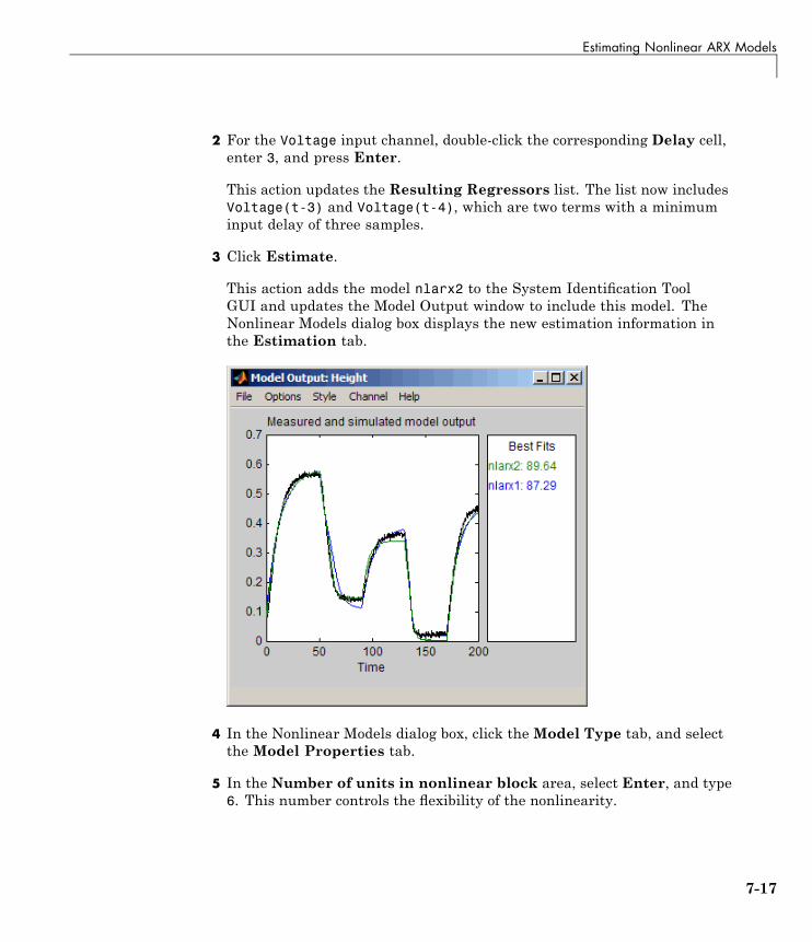
Estimating Nonlinear ARX Models
2 For the Voltage input channel, double-click the corresponding Delay cell,enter 3, and press Enter.
This action updates the Resulting Regressors list. The list now includesVoltage(t-3) and Voltage(t-4), which are two terms with a minimuminput delay of three samples.
3 Click Estimate.
This action adds the model nlarx2 to the System Identification ToolGUI and updates the Model Output window to include this model. TheNonlinear Models dialog box displays the new estimation information inthe Estimation tab.
4 In the Nonlinear Models dialog box, click theModel Type tab, and selectthe Model Properties tab.
5 In the Number of units in nonlinear block area, select Enter, and type6. This number controls the flexibility of the nonlinearity.
7-17
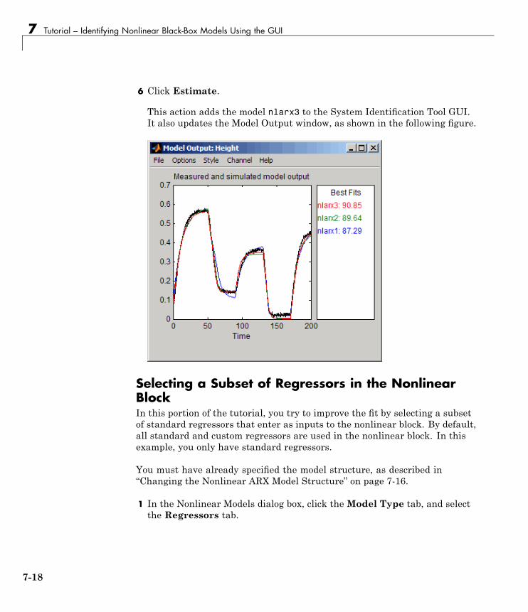
7 Tutorial – Identifying Nonlinear Black-Box Models Using the GUI
6 Click Estimate.
This action adds the model nlarx3 to the System Identification Tool GUI.It also updates the Model Output window, as shown in the following figure.
Selecting a Subset of Regressors in the NonlinearBlockIn this portion of the tutorial, you try to improve the fit by selecting a subsetof standard regressors that enter as inputs to the nonlinear block. By default,all standard and custom regressors are used in the nonlinear block. In thisexample, you only have standard regressors.
You must have already specified the model structure, as described in“Changing the Nonlinear ARX Model Structure” on page 7-16.
1 In the Nonlinear Models dialog box, click the Model Type tab, and selectthe Regressors tab.
7-18
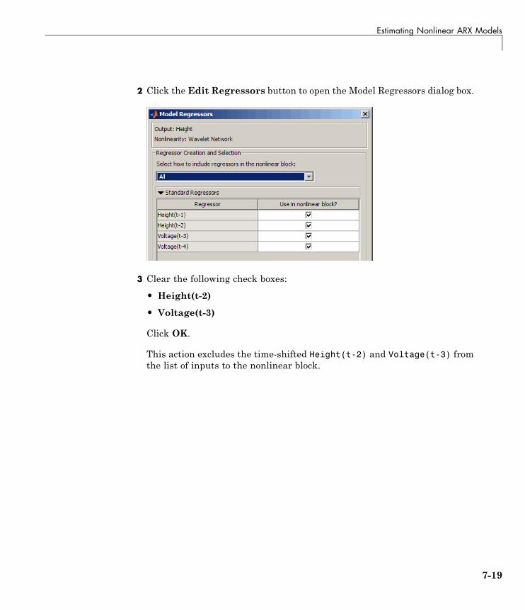
Estimating Nonlinear ARX Models
2 Click the Edit Regressors button to open the Model Regressors dialog box.
3 Clear the following check boxes:
• Height(t-2)
• Voltage(t-3)
Click OK.
This action excludes the time-shifted Height(t-2) and Voltage(t-3) fromthe list of inputs to the nonlinear block.
7-19
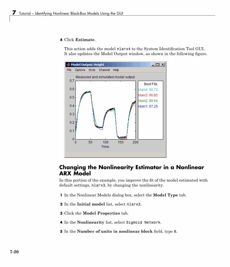
7 Tutorial – Identifying Nonlinear Black-Box Models Using the GUI
4 Click Estimate.
This action adds the model nlarx4 to the System Identification Tool GUI.It also updates the Model Output window, as shown in the following figure.
Changing the Nonlinearity Estimator in a NonlinearARX ModelIn this portion of the example, you improve the fit of the model estimated withdefault settings, nlarx3, by changing the nonlinearity.
1 In the Nonlinear Models dialog box, select the Model Type tab.
2 In the Initial model list, select nlarx3.
3 Click the Model Properties tab.
4 In the Nonlinearity list, select Sigmoid Network.
5 In the Number of units in nonlinear block field, type 6.
7-20
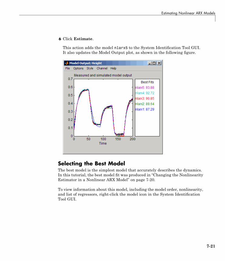
Estimating Nonlinear ARX Models
6 Click Estimate.
This action adds the model nlarx5 to the System Identification Tool GUI.It also updates the Model Output plot, as shown in the following figure.
Selecting the Best ModelThe best model is the simplest model that accurately describes the dynamics.In this tutorial, the best model fit was produced in “Changing the NonlinearityEstimator in a Nonlinear ARX Model” on page 7-20.
To view information about this model, including the model order, nonlinearity,and list of regressors, right-click the model icon in the System IdentificationTool GUI.
7-21
7 Tutorial – Identifying Nonlinear Black-Box Models Using the GUI
Estimating Hammerstein-Wiener Models
In this section...
“Estimating Hammerstein-Wiener Models with Default Settings” on page7-22“Plotting the Nonlinearities and Linear Transfer Function” on page 7-25“Changing the Hammerstein-Wiener Model Structure” on page 7-29“Changing the Nonlinearity Estimator in a Hammerstein-Wiener Model”on page 7-30“Selecting the Best Model” on page 7-33
Estimating Hammerstein-Wiener Models with DefaultSettingsIn this portion of the tutorial, you estimate nonlinear Hammerstein-Wienermodels using default model structure and estimation options.
You must have already prepared the data, as described in “Preparing Data”on page 7-4. For more information about nonlinear ARX models, see
1 In the System Identification Tool GUI, select Estimate > Nonlinearmodels to open the Nonlinear Models dialog box.
2 In the Model Type tab, select Hammerstein-Wiener in the Modelstructure list.
7-22
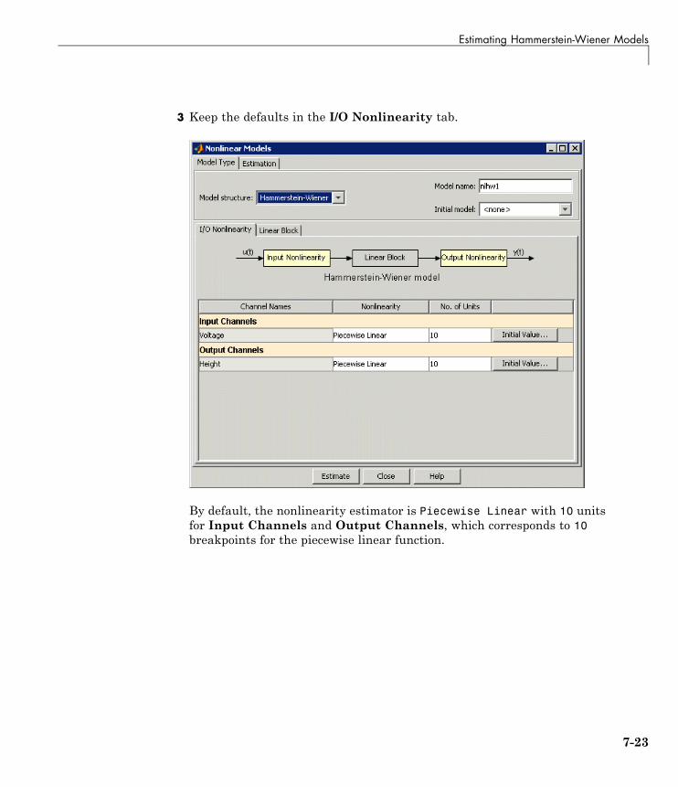
Estimating Hammerstein-Wiener Models
3 Keep the defaults in the I/O Nonlinearity tab.
By default, the nonlinearity estimator is Piecewise Linear with 10 unitsfor Input Channels and Output Channels, which corresponds to 10breakpoints for the piecewise linear function.
7-23
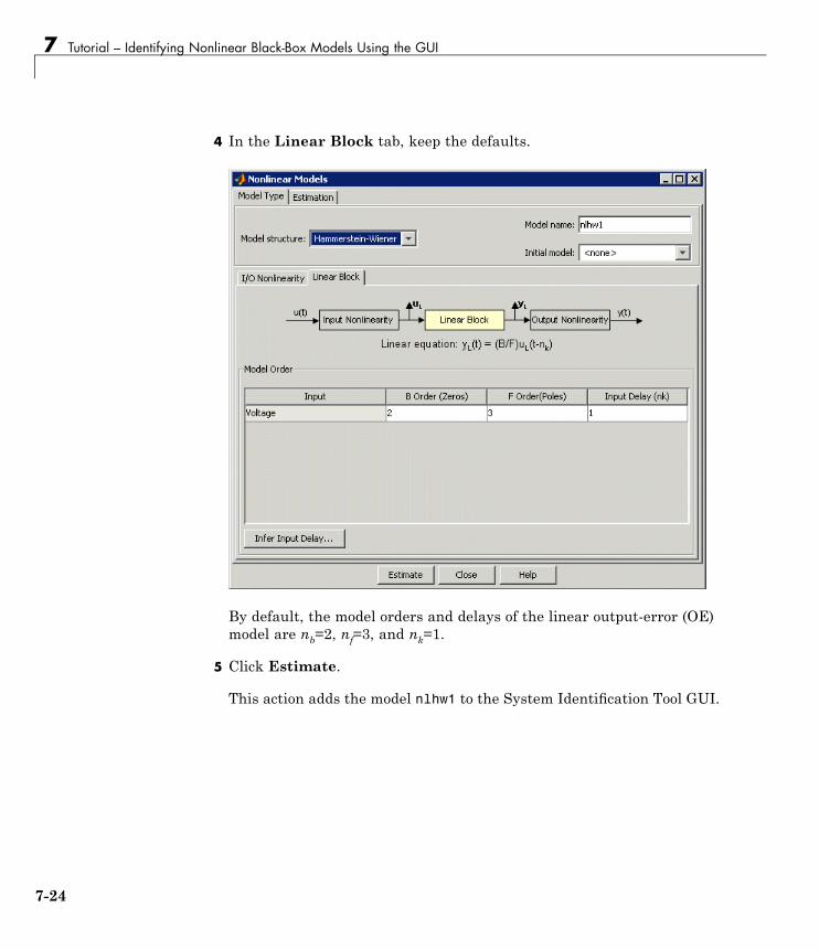
7 Tutorial – Identifying Nonlinear Black-Box Models Using the GUI
4 In the Linear Block tab, keep the defaults.
By default, the model orders and delays of the linear output-error (OE)model are nb=2, nf=3, and nk=1.
5 Click Estimate.
This action adds the model nlhw1 to the System Identification Tool GUI.
7-24
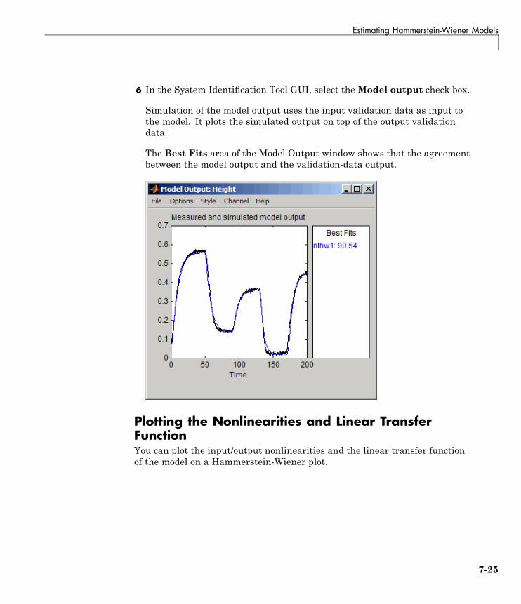
Estimating Hammerstein-Wiener Models
6 In the System Identification Tool GUI, select theModel output check box.
Simulation of the model output uses the input validation data as input tothe model. It plots the simulated output on top of the output validationdata.
The Best Fits area of the Model Output window shows that the agreementbetween the model output and the validation-data output.
Plotting the Nonlinearities and Linear TransferFunctionYou can plot the input/output nonlinearities and the linear transfer functionof the model on a Hammerstein-Wiener plot.
7-25

7 Tutorial – Identifying Nonlinear Black-Box Models Using the GUI
1 In the System Identification Tool GUI, select the Hamm-Wiener check boxto view the Hammerstein-Wiener model plot.
The plot displays the input nonlinearity, as shown in the following figure.
7-26
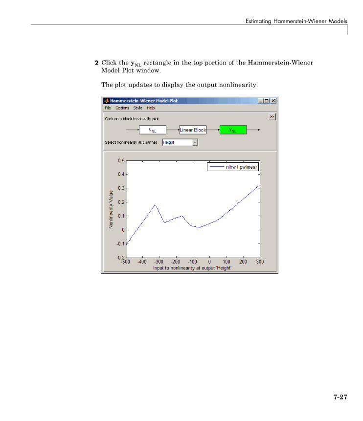
Estimating Hammerstein-Wiener Models
2 Click the yNL rectangle in the top portion of the Hammerstein-WienerModel Plot window.
The plot updates to display the output nonlinearity.
7-27
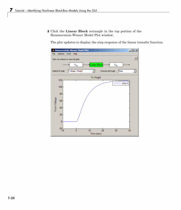
7 Tutorial – Identifying Nonlinear Black-Box Models Using the GUI
3 Click the Linear Block rectangle in the top portion of theHammerstein-Wiener Model Plot window.
The plot updates to display the step response of the linear transfer function.
7-28
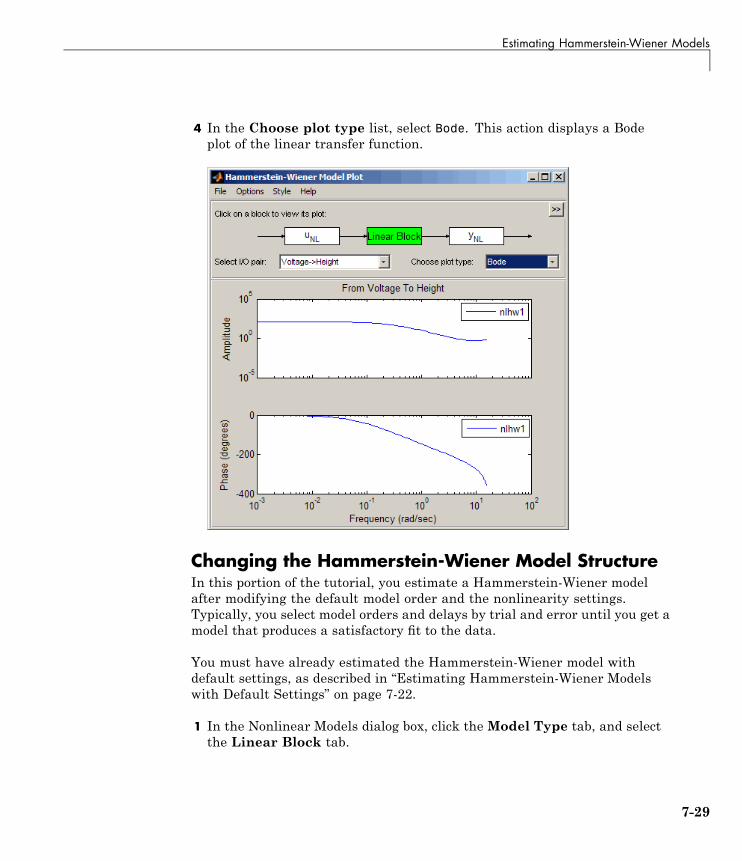
Estimating Hammerstein-Wiener Models
4 In the Choose plot type list, select Bode. This action displays a Bodeplot of the linear transfer function.
Changing the Hammerstein-Wiener Model StructureIn this portion of the tutorial, you estimate a Hammerstein-Wiener modelafter modifying the default model order and the nonlinearity settings.Typically, you select model orders and delays by trial and error until you get amodel that produces a satisfactory fit to the data.
You must have already estimated the Hammerstein-Wiener model withdefault settings, as described in “Estimating Hammerstein-Wiener Modelswith Default Settings” on page 7-22.
1 In the Nonlinear Models dialog box, click the Model Type tab, and selectthe Linear Block tab.
7-29
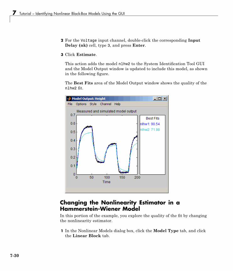
7 Tutorial – Identifying Nonlinear Black-Box Models Using the GUI
2 For the Voltage input channel, double-click the corresponding InputDelay (nk) cell, type 3, and press Enter.
3 Click Estimate.
This action adds the model nlhw2 to the System Identification Tool GUIand the Model Output window is updated to include this model, as shownin the following figure.
The Best Fits area of the Model Output window shows the quality of thenlhw2 fit.
Changing the Nonlinearity Estimator in aHammerstein-Wiener ModelIn this portion of the example, you explore the quality of the fit by changingthe nonlinearity estimator.
1 In the Nonlinear Models dialog box, click the Model Type tab, and clickthe Linear Block tab.
7-30
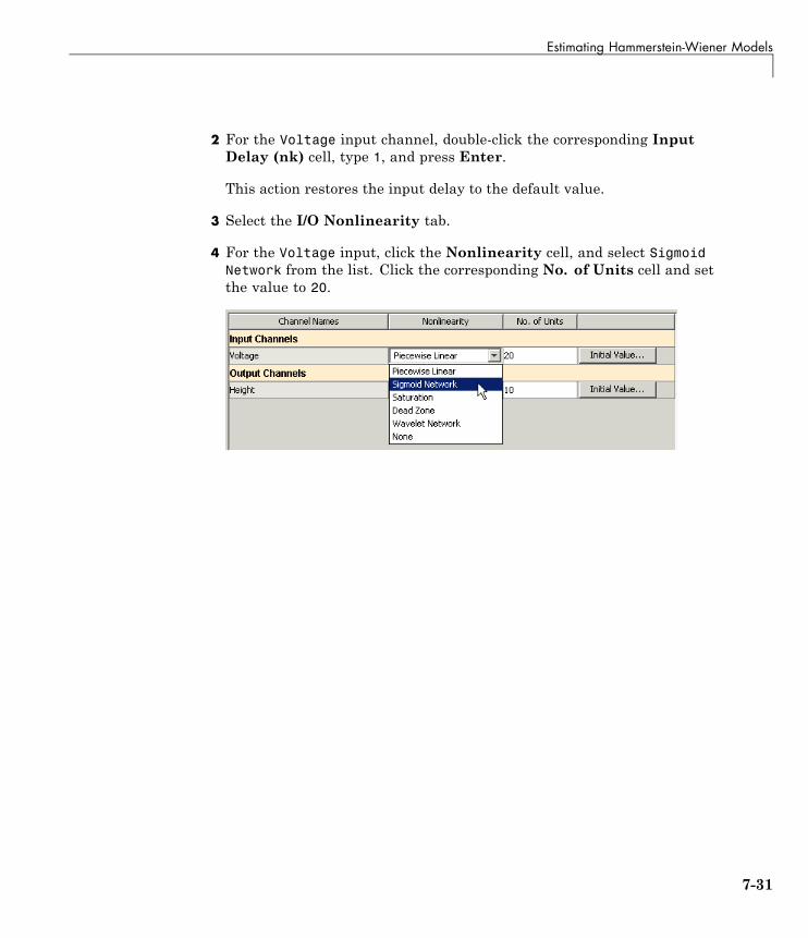
Estimating Hammerstein-Wiener Models
2 For the Voltage input channel, double-click the corresponding InputDelay (nk) cell, type 1, and press Enter.
This action restores the input delay to the default value.
3 Select the I/O Nonlinearity tab.
4 For the Voltage input, click the Nonlinearity cell, and select SigmoidNetwork from the list. Click the corresponding No. of Units cell and setthe value to 20.
7-31
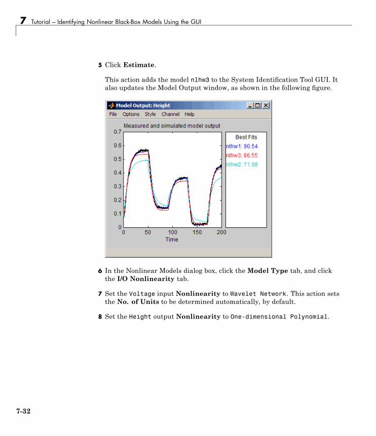
7 Tutorial – Identifying Nonlinear Black-Box Models Using the GUI
5 Click Estimate.
This action adds the model nlhw3 to the System Identification Tool GUI. Italso updates the Model Output window, as shown in the following figure.
6 In the Nonlinear Models dialog box, click the Model Type tab, and clickthe I/O Nonlinearity tab.
7 Set the Voltage input Nonlinearity to Wavelet Network. This action setsthe No. of Units to be determined automatically, by default.
8 Set the Height output Nonlinearity to One-dimensional Polynomial.
7-32
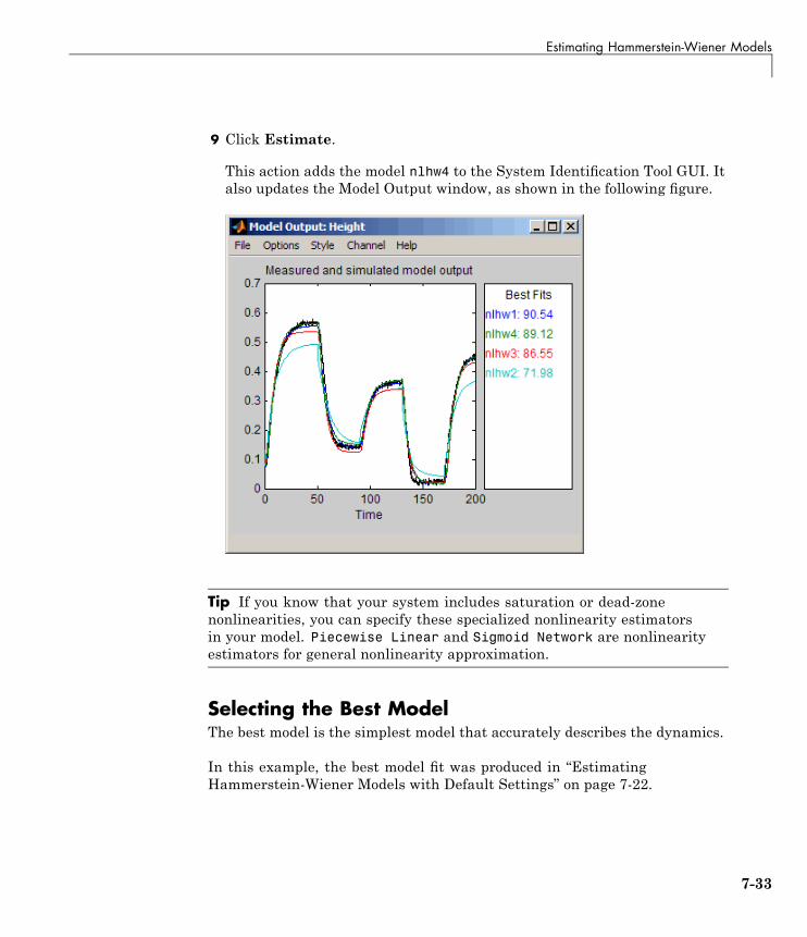
Estimating Hammerstein-Wiener Models
9 Click Estimate.
This action adds the model nlhw4 to the System Identification Tool GUI. Italso updates the Model Output window, as shown in the following figure.
Tip If you know that your system includes saturation or dead-zonenonlinearities, you can specify these specialized nonlinearity estimatorsin your model. Piecewise Linear and Sigmoid Network are nonlinearityestimators for general nonlinearity approximation.
Selecting the Best ModelThe best model is the simplest model that accurately describes the dynamics.
In this example, the best model fit was produced in “EstimatingHammerstein-Wiener Models with Default Settings” on page 7-22.
7-33

7 Tutorial – Identifying Nonlinear Black-Box Models Using the GUI
7-34
Index
IndexAARMAX
estimating using the System IdentificationTool 4-36
ARXestimating at the command line 6-42estimating using Quick Start 4-23
Bblack-box models
advantages 3-7estimating using Quick Start 4-23
Box-Jenkins modelsestimating at the command line 6-42
Ccomparing models
at the command line 6-51
Ddata
creating iddata object 6-8estimation versus validation 3-2importing MAT-file into the System
Identification Tool 4-5importing object into the System
Identification Tool 5-6loading into the MATLAB workspace 4-4plotting at the command line 6-5plotting iddata object 6-5plotting in the System Identification
Tool 4-10preprocessing in the System Identification
Tool 4-10
delayestimating at the command line 6-20estimating using the System Identification
Tool 4-30disturbance model. See noise modeldynamic system 3-2
Eestimation data 3-2exporting models
to MATLAB 4-47to the LTI Viewer 4-49
Ffrequency-response models
estimating at the command line 6-15estimating using Quick Start 4-23
Ggrey-box models
advantages 3-6
Iiddata object
creating 6-8plotting 6-5
importing dataiddata object into the System Identification
Tool 5-6MAT-file into the System Identification
Tool 4-5impulse-response models
estimating at the command line 6-15estimating using Quick Start 4-23
Index-1
Index
Llinear models
estimating at the command line 6-2estimating using the System Identification
Tool 4-2versus nonlinear 3-4
loading data into the MATLAB Workspacebrowser 4-4
LTI Viewer 4-49
Mmodel order
estimating at the command line 6-23estimating using the System Identification
Tool 4-30model parameters
viewing in the System IdentificationTool 4-43
modelschoosing linear or nonlinear 3-4defining structure using idproc 6-31definition 3-2estimating at the command line 6-2 6-31estimating low-order continuous-time
transfer functions 5-2estimating noise models 5-22estimating using Quick Start 4-23estimating using the System Identification
Tool 4-2 5-2using 6-54
Nnoise model 3-3
estimating for model 5-22nonlinear models
when to estimate 3-4nonparametric model
analyzing plots 4-25
Pplotting data
at the command line 6-5in the System Identification Tool 4-10
plotting modelsin the LTI Viewer 4-49
predictionat the command line 6-54
preprocessing datain the System Identification Tool 4-10
QQuick Start
for estimating models 4-23for preprocessing data 4-19
Rremoving data sets from the System Identification
Tool 4-20
Ssimulation
at the command line 6-54using the Simulink software 5-34
Simulink software 5-34state-space models
estimating at the command line 6-42estimating using Quick Start 4-23estimating using the System Identification
Tool 4-35step-response models
estimating at the command line 6-15estimating using Quick Start 4-23
Index-2
Index
System Identification Toolestimating continuous-time models 5-2estimating linear models 4-2estimating models using Quick Start 4-23exporting models to MATLAB 4-47exporting models to the LTI Viewer 4-49removing data sets 4-20saving sessions 4-20starting 2-3 4-4versus command line 2-2
System Identification Toolbox productabout 1-1demos 1-5documentation 1-5related products 1-7resources 1-9steps for using 2-4using with Simulink software 5-34
Ttransient-response models
estimating at the command line 6-15estimating using Quick Start 4-23
trash 4-20
Uusing the System Identification Toolbox
product 2-4
Vvalidating models
at the command line 6-36using the System Identification Tool 4-39
validation data 3-2
Index-3

![· LTPDA Toolbox 7/5/10 6:31:06 PM] LTPDA Toolbox Getting Started with …](https://static.fdocuments.net/doc/165x107/60a8833f505b3c441c582908/-ltpda-toolbox-7510-63106-pm-ltpda-toolbox-getting-started-with-.jpg)