UNLV Retrospective Theses & Dissertations

1-1-1990

System identification of a hydraulically-actuated robot System identification of a hydraulically-actuated robot

Andreas Otto Ranz University of Nevada, Las Vegas

Follow this and additional works at: https://digitalscholarship.unlv.edu/rtds

Repository Citation Repository Citation Ranz, Andreas Otto, "System identification of a hydraulically-actuated robot" (1990). UNLV Retrospective Theses & Dissertations. 129. http://dx.doi.org/10.25669/7jlv-3m0n

This Thesis is protected by copyright and/or related rights. It has been brought to you by Digital Scholarship@UNLV with permission from the rights-holder(s). You are free to use this Thesis in any way that is permitted by the copyright and related rights legislation that applies to your use. For other uses you need to obtain permission from the rights-holder(s) directly, unless additional rights are indicated by a Creative Commons license in the record and/or on the work itself. This Thesis has been accepted for inclusion in UNLV Retrospective Theses & Dissertations by an authorized administrator of Digital Scholarship@UNLV. For more information, please contact digitalscholarship@unlv.edu.

INFORMATION TO USERS

This manuscript has been reproduced from the microfilm master. UMI films the text directly from the original or copy submitted. Thus, some thesis and dissertation copies are in typewriter face, while others may be from any type of computer printer.

The quality of this reproduction is dependent upon the quality of the copy submitted. Broken or indistinct print, colored or poor quality illustrations and photographs, print bleedthrough, substandard margins, and improper alignment can adversely affect reproduction.

In the unlikely event that the author did not send UMI a complete manuscript and there are missing pages, these will be noted. Also, if unauthorized copyright material had to be removed, a note will indicate the deletion.

Oversize materials (e.g., maps, drawings, charts) are reproduced by sectioning the original, beginning at the upper left-hand corner and continuing from left to right in equal sections with small overlaps. Each original is also photographed in one exposure and is included in reduced form at the back of the book.

Photographs included in the original manuscript have been reproduced xerographically in this copy. Higher quality 6" x 9" black and white photographic prints are available for any photographs or illustrations appearing in this copy for an additional charge. Contact UMI directly to order.

UMIU niversity M icrofilms international

A Bell & H owell Information C o m p a n y 3 0 0 North) Z e e b R oad , Ann Arbor, Ml 4 8 1 0 6 -1 3 4 6 U SA

3 1 3 /7 6 1 -4 7 0 0 8 0 0 /5 2 1 -0 6 0 0

Order N um ber 1844904

System identification o f a hydraulically-actuated robot

Ranz, Andreas Otto, M.S.

University of Nevada, Las Vegas, 1991

UMI300 N. Zeeb Rd.Ann Arbor, MI 48106

SYSTEM XDEMTZFIC&TION OF A HYDRAULICALLY-ACTUATED ROBOT

byAndreas Otto Ranz

A thesis submitted in partial fulfillment of the requirements for the degrees of

Masters of Science in

Mechanical Engineering

Department of Mechanical Engineering University of Nevada, Las Vegas

May, 1991

The thesis of Andreas Otto Ranz for the degree of Masters of Science in Mechanical Engineering is approved.

Prof. William Culbreth, Ph.D., Chairperson

/Prof ./James Cardie, Ph.D, Examining Committee Member7i-i-X.- x-y

Prof. Samir Moujaes, Ph.D, Examining Committee Member

Prof. Evangelos Yfantis, Ph.D, Examining Committee Member

Ronald W. Smith, Ph.D., Graduate Dean

May, 1991

11

ABSTRACT

A feedback control system has been developed to operate an elastic robot arm. This work was funded by a grant from the U.S. Army Research Office. The goal of this investigation was to experimentally determine the operating curves, performance plots, and flow coefficients needed to produce an appropriate servovalve signal when operating the hydraulically-actuated robot arm. Through the assimilation of data collected in the laboratory the parameters were determined.

Ill

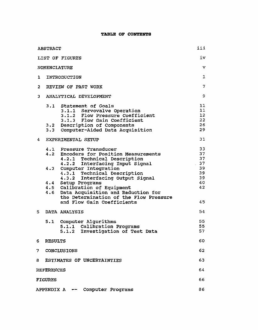
table of CONTENTS

ABSTRACT iiiLIST OF FIGURES ivNOMENCLATURE v1 INTRODUCTION 12 REVIEW OF PAST WORK 73 ANALYTICAL DEVELOPMENT 9

3.1 Statement of Goals 113.1.1 Servovalve Operation 113.1.2 Flow Pressure Coefficient 123.1.3 Flow Gain Coefficient 22

3.2 Description of Components 2 63.3 Computer-Aided Data Acquisition 29

4 EXPERIMENTAL SETUP 314.1 Pressure Transducer 3 34.2 Encoders for Position Measurements 37

4.2.1 Technical Description 374.2.2 Interfacing Input Signal 37

4.3 Computer Integration 3 94.3.1 Technical Description 3 94.3.2 Interfacing Output Signal 3 9

4.4 Setup Programs 404.5 Calibration of Equipment 424.6 Data Acquisition and Reduction for

the Determination of the Flow Pressureand Flow Gain Coefficients 45

5 DATA ANALYSIS 545.1 Computer Algorithms 55

5.1.1 Calibration Programs 555.1.2 Investigation of Test Data 57

6 RESULTS 607 CONCLUSIONS 628 ESTIMATES OF UNCERTAINTIES 63REFERENCES 64FIGURES 66

APPENDIX A — Computer Programs 86

APPENDIX B — Tables and Graphs of Results 13 2Section 1; Data Tables of Results 13 3Section 2: Graphs of Results 152

APPENDIX C — Equipment Specifications 167

LIST OF FIGURES

Figure Title ^1 Hydraulic Servovalve 672 Elastic Robot Arm 68

3 Hydraulic System 694 System Signal Path 705 Pressure Transducer Schematic 716 Operational Amplifier (AD524BD) 727 Low Pass Passive Filter 738 Wiring Diagram for Pressure

Transducer Side 749 Wiring Diagram for Op-Amp Section 7510 Wiring Diagram for Power Sources 7611 Wiring Diagram for Termination

Panel 7712 Signal Modules 7813 Hardware-Software Connections 7914 Setup Programs Block Diagram 8015 Calibration Programs Block Diagram 8116 Calibration Programs Block Diagram

Continued 8217 Flow Pressure Programs Block Diagram 8318 Flow Pressure Programs Block Diagram

Continued 8419 Actuator of the Robot Arm 85

iv

NOMENCLATURE

Presented here are symbols which are found in more than one location within this report. All symbols are explained in their appropriate section in greater detail.

Symbol DescriptionA/D Analog-to-Digital conversionD/A Digital-to-Analog conversion5P Pressure in the hydraulic cylinder6Q Hydraulic fluid flow rate in the actuatorSU Servovalve input displacementI/O Input/OutputK0,I^,K0 Gain coefficients used in the PID controller Kg Flow gain coefficientKc' K/ = 2KgKq Flow pressure coefficient

Lengths of robot arm segments 1,2, and 3 LED Light Emitting DiodeP Pressure difference: Pg - P,P3, P Pressure transducers located on actuator #2AP Pressure difference: P - PjPID Three mode controller including a

proportional, integral, and derivative term; PID controller

Pg Reference pressure, 800 psi

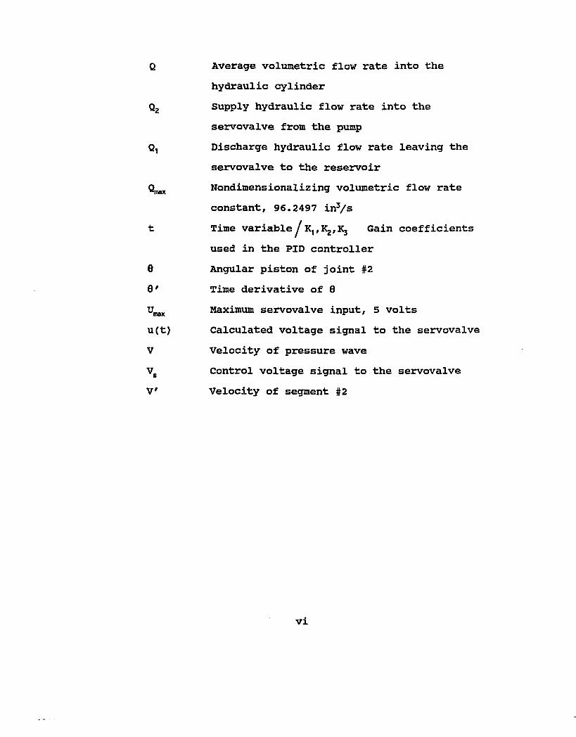
Q Average volumetric flow rate into thehydraulic cylinder

Qg Supply hydraulic flow rate into theservovalve from the pump

Q, Discharge hydraulic flow rate leaving theservovalve to the reservoir Nondimensionalizing volumetric flow rate constant, 96.2497 in^/s

t Time variable^ K,, Kg, Gain coefficientsused in the PID controller

0 Angular piston of joint #28 ' Time derivative of 8max Maximum servovalve input, 5 voltsu(t) Calculated voltage signal to the servovalveV Velocity of pressure waveVg Control voltage signal to the servovalveV' Velocity of segment #2

vi

CHAPTER 1 INTRODUCTION

Robots and robotics have been a subject of discussion and research for centuries. The earliest reference to a "metal attendant" [5] was an Italian fresco in 1350. Since then there have been many milestones which led to our current technology.

An important development towards the advancement of robotics was the clock. As clocks developed they became more intricate while decreasing in size. This miniaturization helped in the development of computers.Also, the gears and wheels necessary to operate a clock led to the development of a new breed of machines. When the gears and wheels of a machine worked together they could complete mundane and repetitive tasks much faster and more efficiently than humans.

During the eighteenth century the industrial revolution began to place unrealistic demands on people working in factories. Machines which used the new power sources, new tools, and new mechanisms developed during this period were able to complete repetitive tasks without risk to humans. They also were more cost effective.

During the Industrial Revolution the terms automation and automatic became prominent. The term was introduced by Karel Cupek in a play, "Rossum's Universal Robots" [5], in 1920. Five years later, the term "robot" appeared in an

2English dictionary. The word "robot" was derived from the Slavik word "robota", meaning heavy work. The Robot Institute of America defines a robot as: "A programmable, multifunction manipulator designed to move material, parts, tools or specialized devices through variable programmed motion for the performance of a variety of tasks." [1 2 ]

Robots are generally categorized into two groups; those robots which are human in appearance and those robots which closely resemble a crane or arm. Robot arms are generally used in industrial applications while the human-like figures are used in the entertainment field.

Today's robot work largely originates from work carried out following World War II. The research programs started in the 1940's were designed to create remotely controlled robots to handle hazards materials such as radioactive materials. These designs were designated "master-slave" robots. The master manipulator was controlled by the operator, the slave manipulator followed the motion as vigilantly as possible. Soon after this phase of development was complete, the development of "programming" robots to perform repetitive tasks became the number one priority. The rise in interest was due to the coupling of these repetitive task robots with industrial applications. The robots developed were designed to perform the same operation in the same manner without regard to changing conditions. In the 1960's the idea of robots with complicated feedback sensing was explored. The sensing of

3conditions by the robot to variations in its environment remains today a wide and interesting field of research.

The applications for robots and robotics is extensive. Conventional robot arms traditionally have been constructed of nonflexible materials. The use of steel to create rigid robot arms increases their weight and decreases their mobility. Traditional applications for these robot arms have been in heavy industry where neither weight, mobility, nor size is a restriction. In the late 1960's, George C. Devol and associates founded Unimation Inc., which produced a number of robot related inventions [12]. In 1961 the first Unimate robot was applied in industry to tend a die casting machine. Since then industrial applications around the world have been increasing. This project made use of a Unimate robot base.

With the improvement of computer technology, the development of control systems which interface computer control stations and robot arms soon followed. Two main problems arose. During operation of a robot arm it was necessary to measure the forces encountered and to account for them when determining motion and position commands. The other problem was to determine a method which would best combine the desired task with motion and force control.

Their are several power sources available for robots to provide motion and force control to the joints and end- effector. They are electrical, hydraulic, and pneumatic.The robot under investigation in this project used hydraulic

4actuators as the power source. Their are also several control schemes currently being used, among them are open- loop, closed-loop, and servo-controlled. This project used both open-loop and closed-loop control schemes to accomplish its goals.

Lightweight elastic robot arms are involved in diverse applications. In a project funded by the U.S. Army at U.N.L.V., a group of researchers have been at work to construct a controlled, elastic robot arm. The arm has been constructed out of lightweight steel beams to decrease its overall weight and to increase its mobility.

The robot has been designed to lift 100 pounds with elastic arm segments 4 feet long. This six degree-of- freedom robot uses three hydraulic cylinders for actuation.

The elastic behavior of the arm segments introduces vibration and deflection problems that rigid robots do not experience. Popular rigid robots, such as the Puma by Unimate, have multiple rigid segments that do not deform under a load. To measure position of the end-effector or "hand" of the robot, the position of each joint is measured accurately with a joint encoder. In order to prevent any elastic deformation of the rigid arm, the maximum load that the rigid robot may handle is restricted to 10 pounds. With a total weight of 350 pounds, the payload to weight ratio of this commercially-available robot is only 1:35.

The U.N.L.V. robot uses lightweight segments to decrease its overall weight, but movement will cause the

5arms to deflect elastically. The arm also vibrates due to this elasticity. The U.N.L.V. robotics project involves the instrumentation of this robot and the development of a control scheme that will actively cancel unwanted vibrations and correct for elastic deflections. The robot is hydraulically actuated and the performance of these actuators must be modeled to create an appropriate control scheme for the entire robot. In the present work, several hydraulic system parameters are determined and presented. These parameters are essential for the accurate control of the robot.

The arm construction is a smaller, lighter design allowing the entire arm structure to be more mobile than traditional robot arms. The nature of an elastic robot arm allows for lightweight construction but introduces many structural, vibrational, and feedback problems.

The current trends in robotics are towards flexible segments. Robot systems involve many technologies working together. In order for a robot to have flexible multiple task capabilities the mechanical, electrical, computer, and sensing technologies all must work together as one system. The trend in robotics is toward developing systems which can adapt to any task.

The work conducted for this thesis involved the system identification of a hydraulically-actuated flexible robot. Accurate control of the robot required a precise measurement of the dynamic force in each hydraulic actuator for a given

6servovalve input signal. This required the installation of appropriate pressure transducers, the design and construction of an amplifier and filtering circuit, and the creation of a computer program. The program calculated flow coefficients for one actuator as a function of flow rate and load. The project required the development of a PID controller to operate the robot at a constant load. The flow coefficients serve to identify the hydraulic actuators to be used in the development of a more sophisticated control algorithm.

CHAPTER 2 REVIEW OF PAST WORK

Under a grant by the U.S. Army Research Office, the University of Nevada, Las Vegas has conducted a research project involving the design of a controlled elastic robot arm. The overall objective of the research project was to incorporate controls, instrumentation, data acquisition, and structural analysis for controlling a multi-segmented elastic robot arm.

The project involved the modeling, simulation, and real-time control of an elastic robot arm. The analytical model developed accounted for the elastic properties of the robot arm as they effected dynamic properties including vibration, damping, and strain characteristics. This analytical model contained both a mathematical and a visual simulation of the robot arm during motion. The visual simulation was carried out using a high-speed graphics workstation.

Once the modeling was completed, a feedback control system was developed for the robot arm. The feedback system included the appropriate sensors and computer control algorithms. The position of the arm during operation was determined from mechanical encoders located at the joints. Forces experienced by the actuators were sensed by pressure transducers. The information gained through these and other sensing equipment was used in the control algorithms to complete an effective feedback control package.

8Since the beginning of the project, several areas of

research have been completed.(1) A computer program was developed which presented

the work envelope, static forces at each joint, and deflection at each joint (S. Ladkany, and T. Banoura) [6 ].

(2) A computer program was developed on an IRIS workstation which displayed the motion of a four segment robot with three elastic segments and two hydraulic actuators (Culbreth, W.G., and Krueger, A.)[8 ].

(3) A structural analysis of the three links was performed under static and pseudo-dynamic conditions (S. Ladkany, and T. Banoura)[6 ].

(4) The effects of elastic deformation and twist on the links were investigated (S. Ladkany and R. Marceau)[13].

(5) Optimum joint angle trajectory for minimum deformation was investigated (Trabia and J. Hu)[12].

(6 ) Software was developed to control the robot arms motion through analog-to-digital and digital-to-analog converters. The software developed for motion control was dependent upon information supplied by sensors placed on the robot arm.

The dynamic forces applied by the hydraulic actuators was crucial in the control algorithms. The real-time control algorithms required this dynamic information.

The incentive for the present study arose from the need for a mathematical model for the behavior of the hydraulic actuators.

CHAPTER 3 ANALYTICAL DEVELOPMENT

The University of Nevada, Las Vegas conducted research in five distinct areas involving the elastic robot arm; (1) sensory perception, (2) robot control, (3) structural analysis, (4) elastic robot simulation, and (5) system integration and evaluation of system performance. The project in this thesis bridged the following areas:

Sensory PerceptionTo acquire the data essential for completing this phase

of the project it was necessary to have access to laboratory data collected during the robot's operation. Sensory perception was the first important step in developing the overall design. During operation certain parameters such as joint velocity and location were required to either be entered as desired conditions for operation or measured for use in the control algorithms.

The robot was hydraulically actuated. Servovalves controlled the flow speed and direction for each actuator. The nonlinearity of the servovalve operation dictates the need for determining flow coefficients to obtain a known system response based on input to the servovalve.

Robot ControlThe determination of the operating coefficients, flow

10pressure and flow gain, along with closed loop control of the robot arm motion was the objective of this project.

Svstem IntegrationSystem integration naturally followed from the

development of the overall requirements. System integration was needed to integrate sensory perception and robot control. Each separate device within the system had to work together to complete the task. Since there were several individual components needed to acquire the data and perform the proper control commands, great care was taken to insure that the individual parts worked together in an accurate and dependable manner.

113.1 Statement of Goals

The robot arm was actuated by three hydraulic cylinders. The motion of each joint, its direction and speed, were regulated by servovalves which in turn were controlled by a micro computer. The calculation of the output signal to the servovalve from the computer relied upon information from the user and information read in by instrumentation on the robot arm. The control of the robot arm, the measurement of its relative position, and measured time values during operation all combined to yield the flow pressure, K , and flow gain, K , coefficients. These coefficients were necessary for the development of an overall control program that will operate the robot, dampen unwanted vibrations, and correct for elastic deflections.The overall control program is being written by other researchers on the project and is beyond the scope of this work. Determining Kg and K comprised the goal of this thesis.

To accomplish this goal, two test conditions for the entire system were run. The method used to measure Kg and Kq was developed using the equations relating flow, pressure, and displacement. The servovalve operation was a prominent factor in developing these coefficients.

3.1.1 Servovalve OperationThe operation of the servovalve was regulated by the

micro computer and a digital-to-analog, D/A, converter. The

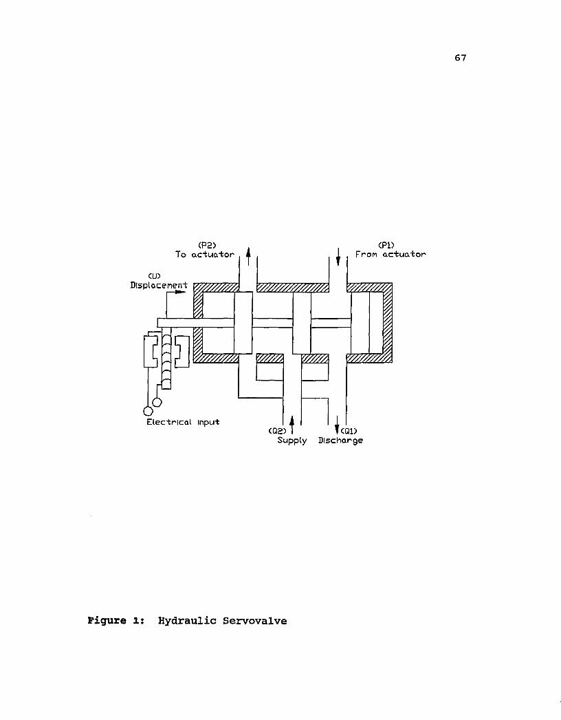
12computer regulated the motion by controlling output voltage signals to the servovalves. A schematic drawing of a hydraulic servovalve is shown in figure 1. It is composed of a piston with carefully arranged landings to coincide with the port width of the actuator. The electrical input into the torque motor caused magnetic forces on the ends of the armature. The input signal caused the displacement of the spool which allowed the hydraulic fluid to flow to the actuator. To the servovalve there is an input supply pressure line, discharge to reservoir line, a line feeding the hydraulic actuator, and a return line from the actuator. Depending upon the input signal to the servovalve, the actuator moved the robot arm in either direction and at a predetermined speed. Hydraulic servovalves which changed the flow direction and flow rate are called flow control valves.

3.1.2 Flow Pressure and Flow Gain CoefficientsThe control of a hydraulic actuator involves varying

the servovalve input, ST3, to achieve a required change in pressure in the hydraulic cylinder, <SP, and flow rate of hydraulic fluid, SQ, according to equation 3.1.

ô(?=-|gxôcr+-^xôP (3.1)

To develop a linearized valve equation, two flow coefficients were needed. The flow equations of a valve are extremely nonlinear, thus, the flow coefficients change with

13operating point. Experimental measurements were used to obtain the valve constants and and Kg. Equations 3.12 and 3.14 contain the equations for both the flow gain and the flow pressure coefficients.

To develop the equations necessary to determine Kg it was assumed that the robot would operate in the range of small displacements around the servovalve operating point as shown in figure 1. The flow rate, Qg, into the actuator increased as the displacement, U, decreased, and decreased as the pressure to the hydraulic actuator, Pg, increased.

à02=KgXàU-Ki:XàP2 (3.2)Looking at the flow rate out of the actuator, Q , we

note a similar relationship. As increased, U and the pressure from the actuator, P , increased, equation 3.3.

àQi=KgX&U+Kix6Pj^ (3.3)The flow equations developed were assumed to be linear.

The actual flow equation coefficients were nonlinear. Coefficients were developed for different conditions because both coefficients were functions of the load on the robot and the configuration of the robot arm.

To simplify the equations, the effects of compressibility were examined. The hydraulic fluid had a bulk modulus of 1.38E+09 N/m^, at l atm, and 20°C.Therefore, it was assumed that the compressibility of the hydraulic fluid was negligible for this application, and indeed, upon review the conditions are well beneath the

14accepted value for incompressibility of a Mach number of 0.3. Equation 3.4 shows the calculations.

Mach=-^

P

1.38x109 =i.54£>4(^)917 s

C>=9.2— Η x0.00i 4 v =0.00945 — mxn l i s

%xO.02542

^°-f°0°0gS5060°°-^^^^-f

Af=lxl0-5 (3.4)

With an incompressible fluid the change in the flow rate entering and leaving became equivalent, equation 3.5.

Ô0i=ô£>2 (3.5)

However, for this case, compressible flow, was assumed to treat the most general case. Instead of using equation3.5 an average flow rate, Q, was defined.

2

To determine add equations 3.2 and 3.3 to obtain

15equation 3.6.

bQ^+bQ^=K^bU+Kgy.bU+ldcX-P^-K'c^^Pz (3 -6)Define a pressure difference, P.

P=P2~Pi (3.7)

Define a flow pressure coefficient, K .

Combine the pressure and displacement terms in equation3.6.

bQ^+bQ^=2K^bU-ldcy.{hP2-bP^) (3.9)

Recall, Kg' = 2Kg and 2Q = Q, + Qj.Reducing equation 3.9.

2bO=2KgXbU-2K^xbP (3.10)

Divide by two and rearrange.

b Q = U ^ b U ) - ( K ^ x b P ) (3.11)

Holding <SP constant.

Equation 3.12 yields the flow gain coefficient, K . Starting with equation 3.11 and holding 6U constant the flow pressure coefficient Kg can be calculated.

16

6Q=-KgXàP (3.13)

<3-i4)

These flow coefficients have a nonlinear relationship throughout the available range of motion. Thus, both the flow pressure and flow gain coefficients were functions of the particular conditions under which the robot was moving. These conditions included the velocity of the arm and the pressure within the hydraulic actuator. The flow pressure coefficient was a function of the speed of motion for the robot arm, while the flow gain coefficient was a function of the desired pressure difference in the actuator. Determination of these experimentally measured coefficients were the focus of this thesis.

Equation 3.14 required a constant actuator velocity in order for the equation to be valid. Also, the flow rate and the differential pressure in the actuator was required through a range of operating points. The nonlinear behavior of Kq and Kg was measured over a range of robot arm joint angles and loads. A simple PID controller was developed to move the robot arm under these desired conditions.

U was defined as the input displacement applied to the spool rod as shown in figure 1. The input displacement regulated the flow rate and indirectly the pressure difference seen by the actuator. The input displacement was controlled by the torque motor, or valve actuator, and by

17the electrical inputs it received from the input source.The input source integrated a micro computer, control software, and appropriate input/output devices. For the calculation of Kg it was necessary to send a predetermined voltage signal, V , from the computer to the servovalve.The voltage signal was sent to the servovalve by the computer through a digital-to-analog converter. A safe speed was required to avoid causing damage to the operator, bystanders, or the robot arm itself. The safe speed range was a subjective speed where minimum velocity of the arm corresponded to 0, and maximum corresponded to 1. For this reason was kept in the range of 0 to 5 volts. This was important when determining K because the closed loop control algorithm may have developed speeds unsafe without this feature. The user entered the speed while testing was in progress for Kg. After the user entered the speed, the safety override check in the computer program ensured a valid speed request. During the experimental test runs, the flow rate and pressure differences were measured.

The flow rate was measured indirectly. Equation 3.15 related Q, the volumetric flow rate into the hydraulic cylinder, to measured values.

0=VxA (3.15)

V is the actual velocity of the hydraulic actuator piston in meters per second. As shown in figure 2, encoders were placed at each joint of the robot to measure its

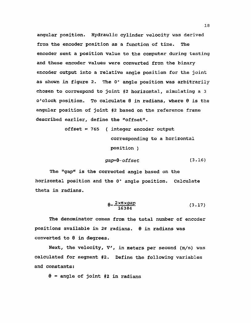
18angular position. Hydraulic cylinder velocity was derived from the encoder position as a function of time. The encoder sent a position value to the computer during testing and these encoder values were converted from the binary encoder output into a relative angle position for the joint as shown in figure 2. The 0" angle position was arbitrarily chosen to correspond to joint #2 horizontal, simulating a 3 o'clock position. To calculate 6 in radians, where 0 is the angular position of joint #2 based on the reference frame described earlier, define the "offset".

offset =7 6 5 ( integer encoder outputcorresponding to a horizontal position )

g a p = Q - o f f s e t (3.16)

The "gap" is the corrected angle based on the horizontal position and the 0° angle position. Calculate theta in radians.

0_-2x7Txgap (3.17)16384

The denominator comes from the total number of encoder positions available in 2 tt radians. 6 in radians was converted to 8 in degrees.

Next, the velocity, V', in meters per second (m/s) was calculated for segment #2. Define the following variables and constants:

6 = angle of joint #2 in radians

190' = angular velocity in radians per second The time derivative was obtained during experimental

measurement by observing the internal computer clock during each test run and calculating d0/dt directly at each encoder position. The length measurements for each segment were done before the tests were carried out. Figure ^ shows the location of each segment. The lengths were measured to be:

= 0.235 meters + 0.001m= 0.546 meters ± 0.001m

Lj = 0.187 meters + 0.001mTo calculate d ' a program was developed which integrated the clock time, the angular position, the length measurements of each segment, and the encoder offset position. 0' became a function of these measured values and 0. See Appendix A, "Computer Programs", section 3.1, subroutine RADIANS.

With 6 ' known, V' was determined using equations 3.18 and 3.19. Equation 3.22 contains the value of V' based upon the length segments of the robot arm, 0, and 0'.

20

1,4 = (Z.ixsin (8 ) H-Lg) (3.18)(L^xcos (0) -1,3) 2

Tl=Z,lX(ZgXCOS(0) +L,xsin(0) ) x0'

a = (LiSin(0) +1,2) P= (L^cos (0) -1,3) 2

(3.20)

T2=V0+P" (3.21)

(3.22)9

The measured pressure values supplied to the actuators by the hydraulic power system were important in determining both Kg and K . A pressure transducer was placed at each end of the hydraulic actuator. The pressure transducer converted the pressure measured in the actuator fluid into an output voltage. To determine Kg and K the pressure differences were measured during the test runs. To convert the voltage signal into pressure with units of pounds per square inch, psi, a calibration ecpaation was needed. Before testing began each pressure transducer was calibrated. The calibration method is explained in section 4.5, "Calibration of Equipment". The outcome of the calibration for pressure transducers 3 and 4 are given in equations 3.23 and 3.24. Each equation relates the final digital voltage signal measured by the computer program through an A/D converter to

21the hydraulic pressure measured at the actuator.

P z e s s u x e T x a n s d u c e x 2 :pressure=-63.2564+206.20x (^*23)

v o l t a g e + 1.3901v o l t a g e ^

P x e s s u x e T x a n s d u c e x A :---------- (3 24)

p x e s s u x e = - 6 6 . 0 6 8 5 +216.3 4 6 5 v o l t a g e

Equations 3.23 and 3.24 were determined by using the measured values and using a least-squares best curve fit method. First, second, third and fourth order degree polynomials were tried to determine the curve fit equation with the lowest standard error.

With all data converted to proper units, was determined. AP is the pressure difference in actuator 2.P4 and P3 correspond to the pressure transducers located on actuator 2 , figure ^3.

0=VxA (3.15)

AP=P4-P3 (3.26)

To nondimensionalize Q, a maximum value, of96.2497 (inVs) was used. For AP, a reference pressure, P , of 800 (psi) was used. and P were specified by theservovalve manufacturer.

Kg was determined from the plots of Q/Q^ax AP/P^ for individual speeds. Kg was the slope of Q/Q^x vs AP/Pg. The measured values and plots are in Appendix B, "Tables and

22Graphs of Results".

3.1.3 Flow Gain CoefficientThe equation necessary to determine the flow gain

coefficient, K , is given in equation 3.27.

(3.27)

Equation 3.27 was valid for a constant pressure difference, P, as defined in equation 3.7. To obtain the flow gain coefficient, K , a system where P was held constant and the flow rate, Q, and the servovalve input, U, were measured during an experimental test run was needed. Since this involved a closed-loop control system an algorithm was developed that read in pressure and encoder data and an output signal to the servovalve. Q was measured in the same manner used for calculating the flow pressure coefficient. From the measurement of the encoder position, length and area constants, and time, the flow coefficient was calculated.

The objective of the closed-loop control algorithm was to hold P constant and allow for the measurement of Q and U. From this point was determined as the slope of Q/Q^^x vs U/Un x* The measurement techniques and data handling were the same as those employed when acquiring the measured data needed for Kg.

The major difference in the techniques developed for acquiring the flow pressure and flow gain coefficients was

23the method in which the robot arm was controlled. The measurement of the test data necessary to compute Kg and K were the same. The procedure in which the robot arm was controlled during the test experimental runs was different. In both cases the user entered specific desired target values for the computer program to accomplish. In the case of Kg the user entered the desired speed at which the robot arm was to move. For K^ the user entered the desired pressure difference in the actuator. In both cases the starting and ending positions of the robot arm was also determined by the user.

In the first case, determining Kg, the speed was chosen by the operator and all other values were measured from sensing equipment. In the case for K , the user choose a desired pressure difference and the control system returned a value for the speed. If the actual pressure difference was within the tolerance range, the controller had reached the desired output. If the actual pressure difference was not within the tolerance range, the control algorithm calculated a new speed.

This method of control for a closed-loop system has been applied to many types of systems including robot arm control. The algorithm was based upon a PID controller. These controllers use a proportional term, an integral term, and a derivative term. The PID controller followed the control algorithm provided by Dorf [10].

A three term controller yielded.

24

u( t) =K^e( t) + ( t) dt+de{t) dt

( 3 . 2 8 )

Where,t - time variableu - PID controller calculated voltage signal

to the servovalve - gain coefficient

Kg - integral coefficient Kj - derivative coefficient e - error between desired and actual

pressure e, - old error valuer - desired output m - actual output

The control algorithm became, e = r - m i = i + (e * t) d = (e - e,)/te, = e

new error integral term derivative term old error = error

u = K,(e) + Kg(i)+ K;(d) : output signal

This algorithm was used in the control program for calculating the appropriate values needed to control the motion of the robot arm. The programs are listed in Appendix A, "Computer Programs". The measured values and

25plots for determining are in Appendix B, Tables and Graphs of Results. was determined as the slope of Q/Q gxvs U/U^x-

263.2 Description of Components

Hydraulic SystemThe elastic robot arm was built with a UNIMATE

industrial robot as the foundation as shown in figure ^ . Motion about each joint was controlled by a hydraulic actuator regulated by a servovalve, The waist rotation actuator was connected through a rack and pinion gearing system to transfer linear motion to rotary motion.

The hydraulic pressure was developed by a vane-type pump driven by a 10-hp electric motor. The hydraulic fluid was contained in a reservoir. The fluid was drawn in to the pump from the reservoir. The hydraulic fluid traveled through a filter and into a manifold. There was an unloading valve in the base manifold which sustained the hydraulic pressure between 750 and 950 psi. The fluid from the unloading valve traveled through a check valve and into the accumulator.

From the base manifold, pressurized fluid was supplied to the servovalves. All actuators were bidirectional and the servovalves responded to an input signal by regulating the quantity of flow and the direction of motion. The input signal was controlled by the software developed for this project on the microcomputer. The input voltage, speed control, and direction values were determined by the needs of the user through the use of the control program. The control program sent the appropriate voltages to the

27servovalve through the digital-to-analog converter and termination modules. The termination module allowed for both analog and digital inputs and outputs to be connected at one central location. All the incoming and outgoing signals were connected through termination panels and mounted into a central rack system.

Unimate RobotThe robot arm investigated was an elastic robot arm.

In the past, robot arms have been constructed of heavyweight materials. They were generally on an immoveable platform or base. Being made of a heavyweight material, the joints were rigid and by the use of location encoders the position was determined easily and accurately. The problem of oscillatory and vibrational motions were minimized by the rigid segments. An elastic robot arm was constructed of lightweight materials. The lightweight materials allow for increased mobility and applications where weight is a concern. However, the elastic robot arm design introduced some unique problems. The two main problems were three dimensional deformation and greatly increased oscillatory motion. The control and modelling of an elastic robot arm must account for these characteristics.

To accomplish the goals set out by this project an elastic robot arm was constructed. The base, which contained the main power source and hydraulic components, was constructed by Unimate. The actual segments, sensing

28devices, and control equipment was built at the University of Nevada, Las Vegas.

293.3 Computer-Aided Data acquisition

The necessary data to determine the flow pressure. Kg, and flow gain, K , coefficients was measured during test runs. The test runs varied the conditions under which the robot arm performed. The conditions were varied throughout the expected range of operation. The required information to run these tests came from transducers.

Several information sources were required to collect all the data. The necessary information sources were as follows:

Input SourcePosition of the robot arm: Encoders.Pressure difference in the the actuators:

Time during tests:

Speed of motion:

Pressure transducers.Internal computer clock.Set by user in program. Measured by differentiating encoder reading with time.

All of these inputs were required to complete the data acquisition phase of this project.

Input SourcesData input was received from the joint encoders and the

30pressure transducers. The signals from the encoders and transducers passed through various signal processing devices before reaching the final destination, the computer, see figure 4. Once the information had been obtained during test runs the input information was reduced to yield and

kq'

Output signalHydraulic actuator control was accomplished by sending

the appropriate voltage signal to the servovalve. The output signal was computed by the program C0NTR0L4.C and converted to an analog output voltage by the PCI-20019M module.

31CHAPTER 4

EXPERIMENTAL SETUP

There were several projects involved in the research and development of the elastic robot arm. This project focused on the development of a technique to control the elastic robot arm.

The information gained from this project was part of the overall research and development concerning the elastic robot arm. The development of the data acquisition and reduction schemes accounted for the need to integrate with past, present, and future projects involved with the robot arm.

To accomplish the acquisition of data essential for this project, the following experimental studies were made.

1) Calibration of each pressure transducer to determine the relationship between servovalve voltage input and pressure.

2) The following procedure was used in the laboratory to find the pressure coefficients.a) Determine which segment of the

robot arm to control.b) Control the voltage signal sent to the

servovalve in order to control the speed of the actuator.

c) Determine of the encoder position.d) Determine of the pressure at each end

32of the actuator,

e) Determine of the time at each input reading.

The data acquisition system included several distinct components to obtain the required data.

334.1 Pressure Transducer

The pressure transducers used were manufactured by Omega as shown in figure 5. The technical information concerning the pressure transducers is supplied by Omega and is included in Appendix C.

The pressure range in which the actuators operated was approximately 0 to 1000 psi, with a maximum pressure of 2 000 psi. The placement of the transducers was situated as close to the ends of the actuators as possible.

All six transducers were the same model from Omega ( P X -

3 02). They were constructed with flat stainless steel diaphragms designed for low pressure levels. The pressures developed by the actuators for the robot arm were considered in the low range.

Strain Gage CharacteristicsThe PX-302 transducers were constructed using strain

gages bonded to the diaphragm by epoxy. The pressure seen through the inlet on the transducer caused a deflection of the diaphragm which was sensed by strain gages arranged as a Wheatstone bridge. By applying a constant voltage source to the bridge, a change in resistance caused a change in output voltage proportional to the input pressure. With the pressure transducers in place it was possible to take the desired pressure measurements.

Operation

34The pressure transducers were connected into the

overall system and the power sources. They were also connected to the output lines which sent the signal through an amplification circuit, into a termination panel, and to the analog-to-digital, A/D, conversion board in the micro computer. Once the measuring system was operating, each transducer was individually calibrated to yield the relationship between input pressure and output voltage.

Interfacing the Pressure TransducersThe output signals from the pressure transducers were

interfaced through several signal processing devices. The output voltage signals corresponding to the pressure seen in the actuator were too low to be read in by the analog-to- digital, A/D, converter in the computer. A Burr-Brown A/D conversion board was installed into the computer. By building an amplification circuit the voltage signal was amplified into an acceptable range before reaching the A/D board in the computer.

The amplification circuit was designed with the following criteria:

1) Each pressure transducer had its own Wheatstone bridge.

2) Input range - 0 to 100 millivolts.3) Output range - 0 to 10 volts.4) Amplification of approximately 50.5) Circuit board placement was to be outside of robot

35framing.

6) A null offset was needed in each circuit.

The amplification circuit was constructed utilizing an instrumentation amplifier with a fixed gain. Each circuit was placed in a separate metal box containing nine-pin connectors for easy removal and replacement. Figure 6 contains a schematic of the amplification circuit. Figure 7 shows the circuit used for the low pass passive filter. Appendix C contains the specifications on the instrumentation amplifier.

After passing through the amplification circuit the signals were sent to a termination panel. The signal lines were connected to the termination panel via double shielded wire in order to reduce electrical noise levels. The connection panel, with incoming and outgoing signals are shown in figures 8,9,10, and 11. In order to interface these signals with the A/D board in the computer, the Burr- Brown PCI-2000 Personal Computer Intelligent Instrumentation System, PCI-20010T Analog Termination Panel was used (Appendix C).

After the signals passed through the termination panel, they were sent to the analog-to-digital conversion board in the personal computer. The carrier board allowed up to three modules to directly connect within the computer, figure 10. There were three modules connected to the carrier board, an A/D input board for the pressure

36transducers, another input board for reading in the encoder positions, and a D/A board used for the output voltage to the servovalves.

374.2 Encoders for Position Measurements

Knowing the position of each joint during motion was important for controlling the robot. The encoders sent output signals to the computer through a digital input/output card. This information was converted to a joint angle by the computer.

4.2.1 Technical DescriptionThe encoders used were absolute optical encoders. The

light source, in this case a Light Emitting Diode, LED, was placed on one side of a disk. The disk held a simple code pattern. The code pattern was illuminated by the light source. Sensors on the other side of the disk read the codes as they passed by. The sensors generated a 12-bit digital signal that represented a unique angle for each joint. This information was transmitted to the computer and used in calculating the robot arm joint angles as functions of time.

4.2.2 Interfacing Input SignalThe encoder signal was sent to the computer through a

PCI-20011T termination panel. The panel could accommodate up to 16 channels of digital input/output, I/O. The termination panel was connected to a PCI-M-1 digital I/O module in the computer. The module had a 32 bit bus. Each byte can be either used for input or output. The carrier board, PCI-20041C-3A, was also used to read in the encoder

38signal. All of the encoder positions were read into the computer using the carrier board and the digital module. Figure 13 contains a schematic layout of the input and output signals in conjunction with the interface to the control program.

394.3 Computer Integration

The development of the programs which measured the data and controlled the motion of the robot arm depended upon information gained from all the separate modules and sensors. Several programs were written specifically for this project.

4.3.1 Technical DescriptionThe computer selected was the Dell System 310 as

described below;Computer type: IBM/PC-AT cloneOperating System: DOS 3.30Main Processor: Intel 80386Co-Processor: Intel 80387The computer housed the carrier board and all modules.

It also contained 'Basic' and 'C language compilers.

4.3.2 Interfacing The Output signalThe computer program CNTRLP5.C in Appendix A read in

data from the encoders and pressure sensors and calculated the servovalve voltage necessary to maintain constant joint speed or constant actuator force. The desired output voltage from the program was converted into an analog signal by a 12-bit PCI-2002IM-IA D/A converter and connected to the appropriate servovalve through a PCI-2OOlOT termination panel.

404.4 Setup Progreuns

During the development of the amplification circuit it was desired to be able to observe the output signal from the pressure transducers directly at the computer. This was done to ensure the signals from the pressure transducers were being transmitted to the computer. Several programs were developed for this purpose. Two are presented in this report (Appendix A). The purpose of the program ADPLOT.BAS was to read an analog signal from one of the pressure transducers, convert it to a digital signal and display the signal graphically in real-time. The program generated a tone with a frequency proportional to the input voltage to allow the user to listen for voltage changes at a remote position in the laboratory. This feature was developed to assist the setup process when working at either remote location of the pressure transducers or the amplification circuit.

The purpose of the program AD.15 was to read an analog input signal from each channel, convert to a digital signal, and write the information to a specified output data file. The program was preset to read for a total time of fifteen seconds. The duration for input was easily changed within the program. This program was used mainly in the initial setup stages of the work. Once a signal had been established by the program ADPLOT.BAS a more detailed investigation of the signal was required. AD15.BAS read the incoming signal and wrote the data to specified data files.

41The data file VOLT.DAT contained a counter value which simply kept track of the number of readings during each test run, and all six voltages read during operation. The data file VOLT34.DAT contained outputs of the counter and voltages from pressure transducers three and four. It was intended that by using specific data files containing only the information currently under investigation, a simple method could be developed for viewing the data through a commercial graphics program. This was accomplished and it allowed a detailed look at the incoming signal during the initial setup of the sensors.

424.5 Calibration of Sensors

Upon completion of the data acquisition system including the sensors, amplification circuit, termination panel, analog-to-digital conversion module, and the personal computer, a method for calibration of the pressure transducers was required. For calibration of the pressure transducer system, a known pressure input and the final computer reading transducer voltage were recorded. With these readings it was possible to determine the calibration curve for each individual pressure transducer. The system was tested over a range of pressures and tested for hysteresis.

A dead weight tester was used for the calibration. The dead weight tester was an accurately calibrated instrument which supplied a known output pressure to the pressure transducers. Each pressure was read by the computer 500 times. The program determined mean and standard deviation and calculated the best approximation for the calibration curve.

From the calibration, an equation relating the pressure transducer's output to the actual pressure was determined. These equations are presented in Chapter 5, "Data Analysis".

Data Acquisition for Calibrating the Pressure TransducersThe pressure transducers were calibrated as a system

including the filters, amplifiers, and A/D board. The calibration program CAL.BAS was designed specifically to

43calibrate one pressure transducer at a time. Before entering the voltage signal from the pressure transducer, the program asked for the channel to be read, the number oftimes the channel was to be read, the known pressure inputvalue, and the name of the output data file. For this report each known input pressure was read 500 times. After entering the data, the program calculated the mean and standard deviation and wrote all the information to a disk file.

The steps in calibration were:1) The program CAL.BAS was run.2) The input pressure at 0 psi on the dead

weight tester was set.3) The known pressure from the dead weight

tester was entered.4) The program read 500 pairs of data for each

pressure input and calculated the mean and standard deviation.

5) The pressure was incremented by 100 psi on thedead weight tester. The values used for calibration were incremented by 100 psi from 0to 1500 psi and down again.

Data Reduction for CalibrationOnce the information relating the pressure to the

output voltage signal was obtained, several programs were written to find the order of the best fit curve by the least

44squares method. Appendix B, sections b and c, contain the final data showing the best fit for pressure transducers three and four.

454.6 Data Acquisition and Reduction for the Determination

of the Flow Pressure and the Flow Gain CoefficientsA control program was developed by Dr. M. Trabia and

Eric Emerson to control the movement of each actuator. The program user entered which actuator to move, the final encoder position, and a relative speed based on a scale of 0 to 1. The program sent the appropriate voltages to the servovalves, and read the encoder position. This program formed the foundation for the control program that was developed during this project.

Data Acquisition for the Flow Pressure CoefficientCNTRLP4.C allowed the user to choose which actuator to

operate during the testing. It also allowed for the selection of the speed at which the robot arm moved, the direction of motion, and starting and stopping positions.The speed was controlled on a relative scale of 0.0 to l.O. The scale was designed with the criteria that at 0.0 there was no motion and at 1.0 the speed was a safe allowable maximum speed. The safest allowable speed was decided by the original designers of the program through observation. Once the relative speed was determined by the user, the program calculated an output voltage signal to be sent to the servovalve.

During the early development of the control program (by Eric Emerson and Dr. M. Trabia) one objective of the control program was to accurately start and stop the motion of the

46robot arm at a desired position. This was accomplished by creating a speed profile for the robot arm to follow.

The speed profile was determined by the user at a prompt input in CNTRLP4.C. The profile controlled the manner in which the voltage signal was sent to the servovalve. The signal was sent in three distinct phases. During the first phase, the arm was brought from a resting position to the desired speed at a controlled acceleration, depending upon the user's requirements. The second phase was the constant velocity section which lasted until the joint approached the desired stopping position. In phase three a declining voltage signal was sent to decelerate the arm to rest as close as possible to the desired position.

The position of the robot arm was determined by CNTRLP4.C through the use of an encoder. Each arm had it's own encoder and encoder position range. The starting and ending position for motion was determined by the user and entered into the control program.

Once the actuator number, speed, speed profile, and ending encoder positions were entered by the user, the program began to move the robot arm. The output data from C0NTR0L4.C contained the necessary information needed to begin the data reduction to find K . Contained in the output data file were the following variables:

1) Time: The time at which C0NTR0L4.Cread each input and sent each output value.

472) Thêta: Joint angle.3) Voltage: The voltage sent from the computer

to the servovalve for actuatorcontrol.

4) Vg: The signal voltage from pressuretransducer three.

5) V : The signal voltage from pressuretransducer four.

With the calibration information and the real-time data obtained during the motion of the robot arm, the datareduction for the began.

Data Reduction for the Flow Pressure CoefficientThe first set of programs was used to obtain the flow

pressure coefficient.1) MAIN.BASPurpose: Start with data directly measured from the

control program CNTRLP4.C and finish with the information needed to calculate K .

Input: (RUN_.DAT) Time, theta, voltage to servovalve,voltages from pressure transducers three and four.

Output: (MAIN_.DAT) New time, theta, theta (radians),

(P3-P4)/P„ 0/Qm=x, U/U x-At this point all the information needed to determine

Kg was known. The output values of Q/Q^^ (Pg-P^)/Pg are plotted in Appendix B.

This process was repeated for ten different speeds.

48The speeds were determined by the relative speed ratio entered by the user (0 to 1). These ten values of the flow coefficient were then plotted against in Appendix B.Several linear and non-linear approximations were tried.The programs that accomplished this were as follows, and are contained in Appendix A, Computer Programs.

2) NTHORDER.BASPurpose; - Read in a set of x(i) and y(i) data pairs.

Generate a system of N equations in the form;y = Ag + A^*x + Ag*x^ + ... + A^*x"Input: (KCUl.DAT) Number of data sets, flow

coefficient, , order of approximation to try.Output: (KCU1FIT.DAT) Number of equations in matrix

to be solved, coefficients in equations.3) MATRIXIN.BASPurpose: This program allows the user to input a

matrix corresponding to a set of simultaneous equations to be solved and allows this data to be stored on disk. The matrix is stored in a file with the extension ".mat". Up to 100 simultaneous equations can be solved.

Input: (KCU1FIT.DAT) Number of equations,coefficients in matrix.

Output: (KCUIMAT.MAT) Same as input with different extension.

4) INVERT.BASPurpose: Calculate the solution to "n" number of

simultaneous equations through the use of Gaussian

49elimination.

Input: (KCUIMAT.MAT) Number of equations, coefficients in matrix.

Output: To the computer screen. The coefficients ofthe approximation, order of the approximation.

5) CALCLINE.BASPurpose: Curve fit the voltage vs pressure data for

the pressure transducers known from INVERT.BAS. Calculate the new pressure at each voltage point and determine the difference between the original data set and the calculated data set.

Input: From the keyboard. Number of data pairs, orderof polynomial, coefficients of approximation.

Output: (KCU1CAL.DAT) Number of data sets, originaldata set, calculated data set.

6) SERROR.BASPurpose: Calculate standard error from the old and new

data sets for voltage vs pressure.Input: (KCU1CAL.DAT) Number of data sets, original

data set, calculated data set.Output: Standard error of the approximation used. At

this point the equation for the flow coefficient in its entire tested range was chosen based on the lowest standard error of the approximations.

Data Acquisition for the Flow Gain CoefficientThe control loop system for K^ was based on a program

50similar to that used for Kg. Specific subroutines which drive the motor, read the time, and read the encoder position were used. Other subroutines were developed for the purpose of controlling the robot arm to measure values for calculating K .

C0NTR0L4.C performed the task of data acquisition for calculating K . The user entered the desired pressure difference in the actuator. The program made all the measurements and calculations needed to control the motion of the robot arm and for determining K .

Once the desired pressure difference in the actuator was entered by the user, the program began the closed-loop control system. Before entering the control loop, the values needed in the PID controller were set. The PID controller operation is explained in Chapter 3, section 3.1.3, Flow Gain Coefficient. There were three PID coefficients needed by the program. The values set in the program were found by trial-and-error. To determine them, two of the PID coefficients were held constant while the third was varied. A series of trial runs were made to determine the lowest standard deviation between the pressure controlled by the PID controller and the desired pressure, while changing each coefficient.The values used were:

K, = 0.01 gain termKg = -0.01 derivative termKj = 0.01 integral term

51time = 1 time coefficient

The PID algorithm calculated the appropriate output speed based on the desired and actual pressure differences. The control loop checked to determine which direction the arm was to be moved. The program then checked to make sure the speed was within the proper safety range (0 to 1). With a corrected speed determined, the subroutine DRIVE_MOTOR was called. DRIVE_MOTOR sent the speed and direction signals to the servovalve.

The encoder position and internal clock time were read. A position check was done to control the point where arm motion was stopped. A high encoder and low encoder position were preset as limits of motion. The following listed values were written to disk.

1) Time: The time at which CNTRLP5.C read eachinput and sent each output value. The time was based on the internal computer clock beginning between a value of 00:00 and 60:00 seconds and ending when operations are completebetween the values 00:00 and 60:00 seconds. The cyclicnature of this method of time determination presents problems which were controlled in a data reduction program.

2) Theta: Encoder position.3) Voltage: The voltage sent from the computer

to the servovalve for actuator control.4) APflctuai' The pressure difference across the

actuator.5) Error: The difference between the desired and

52actual pressure differences.

Data Reduction for the Flow Gain CoefficientThe second set of programs was developed to obtain the

flow gain coefficient. The control program containing thePID control algorithm output the data files X_.DAT. Each data file was designated a number which corresponded to particular testing conditions (APPENDIX B).

(1) MAIN2.BASPurpose: With data directly from the control

program C0NTR0L4.C and finish with information to calculate the flow gain coefficient.

Input: (xf.DAT) Time, theta, actual pressuredifference, calculated speed signal to the servovalve,error.

Output: Corrected time, theta in radians, actualpressure divided by reference pressure, flow rate divided by maximum flow rate, and velocity divided by maximum velocity.

(2) SEMOD.BASPurpose: Read in data from MAIN2.BAS Assume a linear

profile and use the least squares method to calculate the coefficients in the equation: y = mx + b. Also, calculate the standard error.

Input: MAIN2.BAS, Number of data sets, original dataset, calculated data set.

Output: Best fit equation through the test run valuesof the flow gain coefficient for arm travel both up and

53down. Standard error was also provided. This ended the data reduction for the flow gain coefficient. The resulting graphs are in Appendix B.

54CHAPTER 5

DATA ANALYSIS

After all of the experimental data had been collected, the next step was to develop the necessary procedures to study the data. Due to the large amount of data required and collected during acquisition, computer programs were a major part of the analysis procedure.

555.1 Computer Algorithms

To manage the data supplied from the experimental runs, several data reduction programs were developed. It is easiest to examine them in order of operation. The overall strategy was to generate a step by step process which could be implemented on the experimental data. The programs were written in separate blocks due to their size, the origin of the source code, and the lack of available integration techniques between different computer languages.

5.1.1 Calibration ProgramsThe data reduction programs used for calibration were

all written in the computer language 'Basic*, Appendix A.The software used was Microsoft Quickbasic. Due to the nature and the appearance of the calibration data, the calibration curves for pressure transducers three and four were assumed to be linear. Based on this assumption a program named SE.BAS was developed. The purpose of this program was to read in a data file, in this case the data created by the calibration program CAL.BAS, assume a linear profile, and use the least squares method to calculate the coefficients in the equation;

y = mx + b.In the above equation, y represents the voltage from the pressure transducer, m and b are the unknown coefficients, and X represents the voltage read by the computer. The program also calculated the standard error between the

56approximated and the measured data set. It was discovered through the use of SE.BAS that the assumed profile yielded a standard error of 3.47 (psi) for pressure transducer three, and that pressure transducer four had a standard error of1.6 (psi). These values for the standard deviation showed that the linear profile assumed for the data was not acceptable for this project. A series of programs were written to include higher order approximations for the calibration data.

Appendix B contains the original calibration data, the best fit approximations, and standard errors for pressure transducers three and four. Appendix B also contains a comparison of the original data with the calibrated data, and the percent standard error. Each pressure transducer was calibrated independently to yield its own approximation equation.

The order of the approximation equation was determined by the lowest standard error among the approximations tried. The coefficients for 1st, 2nd, 3rd, and 4th order approximations for pressure transducer 3 and for pressure transducer 4 is in Appendix B. The equations determined to be the best fit approximations were:

Transducer 3: y = -63.25641 + 206.2061X + 1.390144x2Transducer 4: y = -66.06855 + 216.3465X

X = transducer output voltage (volts) y = true pressure (psi)

This completed the data analysis phase for the

57calibration of the pressure transducers.

5.1.2 Investigation of Test DataAfter the system had been calibrated, the experimental

measurements began. There were two coefficients. Kg, flow pressure and flow gain, K , which were calculated from experimental data.

The first coefficient. Kg, was derived from experimental data produced by the program CNTRLP5.C. The output from CNTRLP5.C had the following values.

T ; time from internal clock 6 ; angular positionVg : voltage signal to the servovalvePj ; pressure from pressure transducer 3P : pressure from pressure transducer 4

The experimental data was analyzed with several programs. A listing of the programs is in Appendix A. The program MAIN.BAS has several subroutines which are responsible for specific tasks. The final output of MAINl.BAS yields all the data necessary to calculate the flow pressure coefficient.

Subroutine 1; COMBINEThe output of the internal clock was on a 60 second

cycle. When the experimental data was taken, the clock time was written to disk. Converting the repeating 60 cycle clock time into a continuous time which starts at 0 and ends at the conclusion of the test run was done here. Also,

58converting the output pressure voltages from pressure transducer three and four was done here. To convert the data, the calibration equations derived for each pressure transducer were used.

Subroutine 2 : RADIANSThe output of the encoder is an encoder position in the

range from 0 to 16,384. The program converted the encoder position to a relative angle in radians.

Subroutine 3 : DIFFERThe derivative of 0 was calculated in this program. 6

is the angular position, ©' is the angular velocity. The program called the routine DIFFERENTIATE to do the actual calculations. The differentiation was done using a sixth order polynomial, forward interpolation method. The coefficients for the finite difference approximation were provided by Al-Khafaji and Tooley, [1].

Subroutine 4 : VELOCITYThe velocity of the joint was calculated in this

section. Entering 8, the angular position, and 6', the angular velocity, the routine calculated the volumetric flow rate in^/s.

Subroutine 5 : FLOWThe flow rate, Q, was determined using information from

the above subroutines. With the flow rate known, the last calculations included AP. AP is the pressure difference between pressure transducer 3 and pressure transducer 4.The nondimensionalized values of 0/0 ^ and AP/Pg were

59calculated and written to disk. From the plot of Q/Q^y^ vs AP/Pg the flow pressure coefficient was determined.

Subroutine 6: LSMLSM uses a least squares method to determine the best

fit approximation for the slope of Q/Q^^ AP/Pg. The slope of each curve corresponded to Kg.

The second coefficient, K was derived from experimental data produced by the program C0NTR0L4.C. The output from C0NTR0L4.C had the following values.

T ; time from internal clock 6 : encoder positionVg : voltage signal to the servovalve

^ actual • actual pressure difference in the actuator

error : desired pressure difference minus theactual pressure difference

The experimental data contained enough information to calculate K for each operating point tested. The program MAIN2.BAS, Appendix A, contained subroutines which calculated K . Subroutines one through six are identical to those used for calculating Kg with several variables changed to calculate K .

Kq was determined from the slope of O/Q^ax AP/Pg for varying servovalve voltage.

60CHAPTER 6 RESULTS

The objective of this project was to control the robot arm in order to measure values during operation which yielded the flow pressure, K , and flow gain, K , coefficients.

The flow pressure coefficient has been determined for the robot arm for a range of operating points. The operating points for determining the flow pressure coefficient involved varying the speed at which the arm moves. The operating points for involved varying the desired voltage output signal to the servovalve.

There are two equations for K , one for the robot arm motion of joint two in the upward direction, the other for motion in the downward direction. The two equations are:

UP: K . = 0.0553 - 3.8643 x (6.1)+ 0.8729 x^ - 0.5379

D O m : = -0.0137 + 0.0557 X (6.2)

Equations 6.1 and 6.2 complete the objective.The second objective was to determine K . There are

two equations relating to the change in pressure difference desired by the user. The two equations are:

UP: K ç = 0.00034169 AP + 0.1866 (6.3)

The objective of this project has been met by providing

61

DOWN: Kg= -0.003 A P + -0.02495 (6.4)

the proper equations for determining the flow pressure and the flow gain coefficients. The techniques developed can also be used to control the other two actuators.

62CHAPTER 7 CONCLUSION

The goal of determining the flow pressure and flow gain coefficients has been achieved. Several computer programs were written to control the robot arm and to take real-time measurements. Data reduction of the information gained during the project yielded two flow pressure and two flow gain equations.

Recommendations for further work include the following proposals. The remaining pressure transducers for actuators #1 and #3 should be connected into the system. The necessary modules for analog-to-digital, A/D, and digital- to-analog, D/A, conversions were installed during this project. The same tests and data reduction schemes should be used to determine the remaining coefficients.

One objective of the overall research being conducted on the elastic robot arm is accurate control of motion for varying load conditions. The relationship between the control signal and the forces in the robot arm is essential for this goal. In the project being completed by Lam [15], the relationship between the motion and the forces of the robot arm are being developed. The relationship between the motion and the control signal to the robot arm have been developed in this report. Combining this information will lead to the relationship between the control signal and the forces in the robot arm.

63CHAPTER 8

ESTIMATES OF UNCERTAINTIES

Start this section here

64

REFERENCES

1. Al-Khafaji, A., and Tooley, John, Numerical Methods in Engineering Practice. Holt, Rinehart, and Winston, Inc., New York, 1986.2. Anderson, Wayne R., Controlling Electrohvdraulic Systems. Marcel Dekker, Inc. 1988.3. Araya, H., Kakuzen, M., Kimura, N., An Automatic Control System for Hydraulic Shovels. Electronics Technology Center, Japan.4. Ashworth, N., Paul, F.W., Computer Control Compensation for Mechanical Clearance in Hydraulic Robot Joint Servomechanisms. Clemson University, South Caroline.5. Asimov, Issac, and Frenkel, Karen. Robots. Machines in Man's Image. Harmony Books, New York, 1985.6. Bannoura, T., and Ladkany, S., "Structural Analysis and Design of a Flexible Three-Link Hydraulically Actuated Robotic Arm," Masters Thesis, Department of Civil and Mechanical Engineering, University of Nevada, Las Vegas,1988.7. Baysec, S., Jones, Rees, "The Comparative Merits of Analogue and Digital Computers in the Simulation of Hydraulically Driven Robot-Manipulators," Proceedings of the Sixth World Congress on Theory of Machines, pages 944- 949, 1983.8. Culbreth, W.G., and Krueger, A., "Computer Simulation of a Three-Link Hydraulically Actuated Robotic Arm," SME Transaction MS89-248, 1989.9. DeSilva, Clarence W., Control Sensors and Actuators. Prentice-Hall, Inc., 1989.10. Dorf, Richard C., Modern Control Systems. Fourth Edition. Addison-Wesley Publishing Company, Inc., 1986.11. Gemmeke, M., Jonckheere, R.E., Performance Study of a Proportional Valve-Controlled Hydraulic Robot Actuator. Mechanical Engineering, Vrije Universiteit Brussel.12. Gerardo, B., and Hackwood, S., Recent Advances in Robotics. Wiley and Sons, Bell Laboratories, 1985.13. Hu, J., and Trabia, M., "Optimal Joint Trajectory Planning for a Robot with Elastic Links," Masters Thesis, Department of Civil and Mechanical Engineering, University of Nevada, Las Vegas, 1990.

6514. Ladkany, S., and Marceau, B., "The Dynamic Response of a Flexible Three-Link Robot Using Strain Gages, Lagrange Polynomials, Fourier Series, and Finite Element Analysis," Masters Thesis, Department of Civil and Mechanical Engineering, University of Nevada, Las Vegas, 1989.15. Lam, E. and Trabia, M., "Modelling of the UNLV-ARO Flexible Robot Using Lagrange's Assumed Mode Method,Symbolic Manipulation and Numerical Simulation," Masters Thesis, Department of Mechanical Engineering, University of Nevada, Las Vegas, 1991.16. Mayne, R.W., Sadler, J.P., Venkataramna, V.,"Modelling of a Hydraulically Actuated Mechanism," Proceedings of the Sixth World Congress on Theory of Machines and Mechanisms, 1983.17. Omega Group. Pressure. Strain and Force. Vol. 26,Omega Group, Stamford, CT, 1989.18. Whitney, Daniel E. "Historical Perspective and State of the Art in Robot Force Control," The International Journal of Robotics Research, Vol. 6, No. 1, Spring 1987.

66

FIGURES

67

<P2)To a c tu a to r 1

(U>Displacement

£oE lectr ica l input

(PI)From a c t u a t o r

(Q2) I 1CQ1)Supply D ischarge

Figure 1: Hydraulic Servovalve

68

Link 2

■ Pressure Transducer 4■■ Actuator 2■ Pressure Transducer 3

/

Figure 2: Elastic Robot Arm

69

Accumulator

R egu latorActuator

Actuator

Actuator

Motor

Pump Cooler

R e se rv o irS ervovalve ] -Up/Down

S ervovalve2-In /O u t

S ervova lve3 -R o ta ry

F i l t e r

Figure 3: Hydraulic System

70

Pressure Transducers 0 - 100 nv

For closed-loop control system Actuator

ServovalveAmplification Circuit

PC1-20010T Termination Panel

PCI-S0019M-1A A/D Conversion

Personal Computer

Figure 4: System Signal Path

71

1 /4 NPT El/32'3/8'

.60'

7/8'f + m w t( nwn 1

-Jicpen. f - nirfrurt )

r 1 15/16'-----

Figure 5: Pressure Transducer Schematic

72

Input O ffse t Null

O utput Signal Common

-15 V

Figure 6; Operational Amplifier (AD524BD)

73

R = 350 ohns

Voltage Inputfrom p ressu re transducer

-O Voltage Output to amplification circuit

- o-C = 1 microfarad

o-

Figure 7: Low Pass Passive Filter

74

P re ssu re T ransducer

Chassis Gnd

pin p lu gpin p lu gSignal +Chassis Gnd

Signal + (White)

Signal - (Green)Signal -

+10 vdc (Red)+10 vdc

(Black)Gnd

Male

Lowpassf i lte r

Figure 8: Wiring Diagram for Pressure Transducer Site

75

Wiring Diagran f o r Dp-Anp Section

9 pin p l u g

Chassis Gnd

9 pin ^ p l u g 4r

Chassis Gnd

+ 15 vdc

- 15 vdc

Signal + (White)

Signal - (Green)

+10 vdc (Red) V outSignal GndGnd (Black)

+ 10 vdcFemale

Gnd

Figure 9; Wiring Diagram for Op-Amp Section

76

&

Chassis Gnd Power Supply•*•15 vdc (Vhite)

-15 vdc (Black)

Gnd (Red)

Gnd (Green)

Vout

Gnd panel•*■10 vdc (Red)

Gnd

^ •US vdc

-15 vdc

^ Gnd

Reoulator Power Supply

Figure 10: Wiring Diagram for Power Sources

77

Signals from Pressure Transducers 3 and 4

Vout Ch. 4o —

Gnd Ch. 4o-Vout Ch. 3O --Gnd Ch. 3

0 — 1

□ Not Used

□ Not Used

Signals to A/D Converter

□— Not Used

— Not Used

__Not Used

□__ Not Used

□__Not Used__Not Used__Not Used__Not Used

1 Q Vin Ch. 4

■ Q Gnd Ch. 4

-o Vin Ch. 3 ^ Gnd Ch. 3

Figure 11: Wiring Diagram for Termination Panel

78

Dlgl-tol

Digital

Analog

Analog

20011T

EOOllT

20010T

20010T

EDOllT

20019M-1A

20D41C-3A

2D004M-1

Send tine voltage^ signal to the servo valves

Read the pressure

Read the encoder position

Figure 12: Signal Modules

79

HARDWARE SOFTWAREControl Program

a- Read th e encoder positions

o-Read th e p ressu re values

Send th e voltage signal

Internal tine Motion direction Joint number

orSpeed

P ressured ifference

orKc values Kq values

Figure 13: Hardware-Software Connections

80

Volt.dat

Screen o u tp u t

ADPLOT - read an anlo signal from one of th e pressure transducers, convert It to 0 digital signal and dislplay as a real-time graph.

AD15 - read an analog signal from one o f th e pressure transducers, convert It to digital signal and write the output to a specified datafile.

Figure 14: Setup Programs

81

s w i t c h ,d a t

nth,da t

n a t , d a t

lnv,dat

CAL - c a l ib ra t ion o f t h e p r e s s s u r e t r a n s d u c e r s

SWITCH - r e o r g a n i z e d a t a f o r m a t , s w i tc h columns from CAL

NTHDRDER - r e a d in a s e t o f X , y d a t a pa irs , g e n e r a t e a s y s t e m o f N e q u a t io n s in t h e form y = Ag + A X +,„+ A x"

MATRIXIN - Input a matrix t o a s e t o f s im u l ta n e o u s e q u a t io n s t o be s o l v e d

INVERT - c a l c u l a t e t h e s o lu t io n t o n number o f s im u l ta n e o u s e q u a t io n s

Continued in Figure 16

Figure 15; Calibration Programs

82

inv.dat

serror.dat

SERRDR - calculate standard from X, y, and ynew data set

CALCLINE - calculate a set of data from the approximation equation supplied by INVERT

Figure 16: Calibration Programs Continued

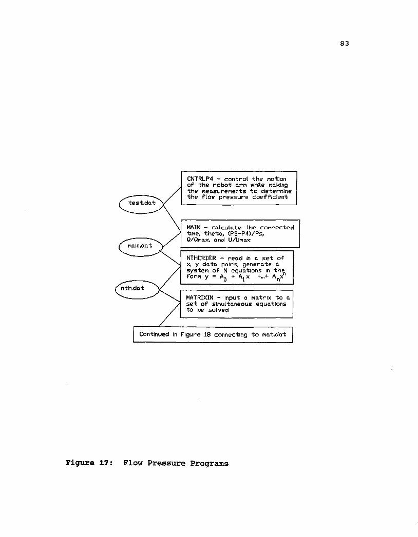
83

nain,dat

Continued In Figure 18 connecting to nat.dat

MATRIXIN - input a matrix to a s e t o f simultaneous equations to toe solved

MAIN - calculate th e co r rec ted time, th e ta , (P3-P4)/Ps,Q/Qmax, and U/Umax

NTHDRDER - read in a s e t of X, y d a ta pairs, genera te a system o f N equations In th ^

CNTRLP4 - control th e motion o f th e rotoot arm while making th e measurements to determine th e flow p ressu re coeffic ien t

Figure 17: Flow Pressure Programs

84

Inv.dat

s e r r o r .d a t

SERRDR - c a lc u la t e s ta n d a r d from X, y, and ynew d a ta s e t

INVERT c a lc u la t e t h e so lu t io n n number o f e q u a tio n s

CALCLINE - c a lc u la t e a s e t o f d a ta from t h e approxim ation eq u a tio n su p p lied by INVERT

Figure 18: Flow Pressure Programs Continued

85

HydraulicP r e s s u eLines

1Hydraulic p r e ssu r e line I

3 /8 ' Tee con n ector

Presure transducer I/O signal wires f o r

p r e s s u r e tr a n sd u cer s

u

Figure 19: Actuator of the Robot Ann

86

APPENDIX A — Computer Programs

87Computer Programs

1) Programs for Experimental Setup1.1 ADPLOT.BAS1.2 AD15.BAS

2) Calibration Programs to Obtain Approximation Equation2.1 CAL.BAS2.2 SWITCH.BAS2.3 NTHORDER.BAS2.4 MATRIXIN.BAS2.5 INVERT.BAS2.6 CALCLINE.BAS2.7 SERROR.BAS

3) Data Analysis3.1 MAIN.BAS3.2 SEMOD.BAS

88

(1) 1.1 ADPLOT.BAS12 • ********** ADPLOT.BAS **********

1

3 ' Purpose: Read an analog signal from one of thepressure transducers, convert to adigital signal and display

5 1 as a real-time graph, with or withoutg I

tone7 * Input: Channel to be read89

1

1Tone Required ('yes' or 'no')

10 ///// Andreas Ranz11 ///// U.N.L.V.12 ///// Spring 199013 1

14 t

15 1

16 1

20 ' Chain merge program "PCIHEAD.BAS" in this location.30 • "PCIHEAD.BAS " loads lines 100 - 159.40 1

50 CHAIN MERGE "PCIHEAD.BAS", 100, ALL60 1

70 1

100 » *** Header File for PCI-20046S BASIC Applications ***101 DEFINT A-E, G-Z102103104105106107108109110 111 112113114115116117118119120 121 122123124

Define the internal signatureDIM VCHK (5) DIM VERS (5)

VERS (1) VERS VERS VERS VERS

(2)(3)(4)(5)

VCHK.L = 5 VERS.L = 5 513 8481 8481 8481 33

Define the PCI-20046S instruction offsets. AUTOGRPH = 12 CNF.AI = 18 CNF.CNTR = 2 4 CNF.DI = 30 CNF.DO = 36 CNF.HDI = 42 CNF.HDO = 48 CNF.RG = 54 CNF.RTD = 60 CNF.TCPL = 6 6 CNF.TRIG = 7 2 CVT.RTD = 78 CVT.TCPL = 8 4 ERR.SYS = 90

89

125 INIT = 96126 READ.CH = 102127 READ.CTS = 108128 READ.FRQ = 114129 READ.SSH = 120130 STAT.CNT = 1 2 6131 STAT.HD = 132132 SYSINIT = 138133 WRITE.CH = 144134 WRITE.GR = 150135 ' Define the PCI-20046S I/O types.136 AI = 1137 AO = 2138 CT = 3139 DI = 4140 DIET = 5141 DO = 6142 DOST = 7143 RG = 8144 TCPL = 9145 TRIG = 10146 RTD = 11147 ' Thermocouple types supported; J K T148 ' RTD ranges supported: 1 2149 '150 DEF SEG = 0 : INTVEC = &H180151 SEGMT = PEEK (INTVEC+2) + &H100*PEEK (INTVEC+3)152 DEF SEG = SEGMT153 ' Check for installed software154 IF (SEGMT <> 0) AND (PEEK (11) = 1) AND (PEEK (12) = &H9A) THEN 156155 PRINT "PCI-20046S not installed or invalid.", CHR$ (7) : END156 CALL AUTOGRPH (VERS.L, VCHK (1), VCHK.L)157 IF (VCHK.L <> VERS.L) THEN 155158 FOR I = 1 TO VCHK.L : IF (VERS (I) <> VCHK (I)) THEN 155159 NEXT I160 '190 '200 ' Dimension variables210 '220 DIM ADATA (10)230 DIM FDATA (10)280 '290 •300 ' Set initial values of variables310 '320 FOR I = 1 TO 6 330 '340 ADATA(I) = 0350 FDATA(I) = 0360 COUNTER = 0

90370 380 390 400 480 490 needed.

NEXT I

500 505 510 520 530 540 550 560 570 580 600 512 630 640 650 700 710 720 730 740 750 760 770 780 800 ' 990 '1000 '1004 '1005 and max 1010 ' 1011 1012", CHN1013 ANS$101410151016 1020 10221023102410251026 1027

GOTO 580 ; ' Jump over the error subroutine until Define the error processing subroutine Error Subroutine --

CALL ERR.SYS (ERROR.CODE) IF ERROR.CODE = 0 THEN 560 PRINT EROR$ ; ERROR.CODE : RETURNI

Error subroutine

END

I I I ICALLI I I IHDWSEG = &HDOOO CALL INIT (HDWSEG)I

EROR$ = "ERROR FOUND GOSUB 500I

Initialize the PCI-200462-1 systemSYSINIT

Define base address of the board Using &HDOOO — for this app

DURING INIT (LINE 760)"

Set up the interface to run the A/D conversion.Read and conversion loop

FLOW = 10 ; FHIGH = 0 : • Set values used+wor min

CLSPRINT : PRINT : INPUT "Input the channel number: INPUT "Would you like the constant tone: (y or n) ",PRINT : PRINT : CLS SCREEN 9 : WINDOWCOLOR 4,11I

I

I

IF ANS$ = "n" THEN DUM = 1 COUNTER = COUNTER + 1 IF C0UNTER>1 THEN 1039 LINE (50,7) - (50,2) : LINE

(0,0)-(619,10)

Begin the data acquisition loop.

(50,2) - (510,2)

91FOR FI = 2 TO 7 STEP .5 ; LINE (50,FI)-(30,FI)1028

NEXT FI1029 LOCATE 3,15 : PRINT "Voltage1030 LOCATE 2,15 : PRINT "ChannelLOCATE 2,25 : PRINT CHN

COLOR 14,111031 COLOR 5,12 14,3 : PRINT " 5 V"1032 COLOR 4,111033 LOCATE 2,411034 LOCATE 3,411035 ' COLOR 4,11 :

LOCATE 8,3 : PRINT "10 v' LOCATE

II

IIPRINT " Minimum voltage PRINT " Maximum voltage

FOR FD = 0 TO 1 STEP .01: LINE (0,FD)- (640,FD) : NEXT FD1036 IF DUM = 1 THEN GOTO 1037 ELSE LOCATE 22,42 ; PRINT"Sound frequency (Hz) :"1037103810391040 1050 1070 1080 1090 1100 ' 1110 1120 1130 1140 114511505!) / GAIN1151FDVOLT = 21153115411551156 1160 1161

PRINT " Average voltageCOLOR 4,11 LOCATE 5,41

Z.CHN = 0 RANGE = 2 GAIN = 1

CALL CNF.AI (CHN, GAIN, Z.CHN, RANGE)EROR$ = "ERROR FOUND DURING CALL.CNF (LINE 1080)" GOSUB 500ICALL READ.CH (AI, CHN, ADATA(CHN))EROR$ = "ERROR FOUND DURING READ.CH (LINE 1120)" GOSUB 500ICOLOR 14,11FDATA(CHN) = ((4095! - ADATA(CHN))*10! / 4096! -FVOLT = FDATA(CHN) : DCOUNTER = 50 + COUNTER: + FVOLT * .5IF FVOLT < FLOW THEN FLOW = FVOLT IF FHIGH < FVOLT THEN FHIGH = FVOLT LOCATE 2,60 : PRINT USING "###.#####" ; FLOW

PRINT USING "###.#####" ; FHIGHPRINT USING "###.#####" ; FVOLT

LOCATE 3,60 LOCATE 3,24 IF COUNTER =

- (DCOUNTER,FDVOLT)1 THEN PSET (50,FDVOLT) ELSE LINE

1162 10 :1163 request1164 100116511691170 119012051206 1210 1220

IF COUNTER = 460 THEN COUNTER = 0 : CLS : FLOW =FHIGH = 0

IF DUM = 1 THEN GOTO 1170: ' Jumping the tone onSOUND FVOLT*1000+100,1

PRINT USING "######"FSOUND = FVOLT * 1000 +

LOCATE 22,65 COLOR 4,11

FSOUND

IF COUNTER = 0 THEN FTOTAL = 0 AND FAVG = 0IF COUNTER = 0 THEN GOTO 1240FTOTAL = FTOTAL + FVOLT : FAVG = FTOTAL / COUNTERLOCATE 5,60 : PRINT USING "###.#####"; FAVG

921230 '1240 GOTO 1016 1250 '1500 END

93

(1) 1.2 AD15.BAS1 ' ********** AD15.BAS **********2 '3 ' Purpose: Read an analog signal from each

input channel. Write digital information in 'VOLT.DAT' andI

' VOLT34.DAT'5 '6 ' Input: Run7 '8 ' ///// Andreas Ranz9 ' ///// U.N.L.V.10 ' ///// Spring 199012 '14 '

15 '20 ' Chain merge program "PCIHEAD.BAS" in thislocation.30 ' "PCIHEAD.BAS" loads lines 100 - 159.40 '50 CHAIN MERGE "PCIHEAD.BAS", 100, ALL60 '70 '100 ' *** Header File for PCI-20046S BASIC Applications ***101 DEFINT A-E, G-Z102 ' Define the internal signature103 DIM VCHK (5) : VCHK.L = 5104 DIM VERS (5) : VERS.L = 5105 VERS (1) = 513106 VERS (2) = 8481107 VERS (3) = 8481108 VERS (4) = 8481109 VERS (5) = 33110 * Define the PCI-20046S instruction offsets.111 AUTOGRPH = 12112 CNF.AI = 18113 CNF.CNTR = 24114 CNF.DI = 30115 CNF.DO = 36116 CNF.HDI = 42117 CNF.HDO = 4 8118 CNF.RG = 54119 CNF.RTD = 60120 CNF.TCPL = 66121 CNF.TRIG = 72122 CVT.RTD = 78123 CVT.TCPL = 84124 ERR.SYS = 90125 INIT = 96

94126 READ.CH = 102127 READ.CTS = 108128 READ.FRQ = 114129 READ.SSH = 120130 STAT.CNT = 126131 STAT.HD = 132132 SYSINIT = 138133 WRITE.CH = 144134 WRITE.GR = 150135 ' Define the PCI-:136 AI = 1137 AO = 2138 CT = 3139 DI = 4140 DIET = 5141 DO = 6142 DOBT = 7143 RG = 8144 TCPL = 9145 TRIG = 1 0146 RTD = 11147 ' Thermocouple types supported: J K T148 ' RTD ranges supported: 1 2149 '150 DEF SEG = 0 : INTVEC = &H180151 SEGMT = PEEK (INTVEC+2) + &H100*PEEK (INTVEC+3)152 DEF SEG = SEGMT153 ' Check for installed software154 IF (SEGMT <> 0) AND (PEEK (11) = 1) AND (PEEK (12) = &H9A) THEN 156155 PRINT "PCI-20046S not installed or invalid.", CHR$ (7) : END156 CALL AUTOGRPH (VERS.L, VCHK (1), VCHK.L)157 IF (VCHK.L <> VERS.L) THEN 155158 FOR I = 1 TO VCHK.L : IF (VERS (I) <> VCHK (I)) THEN 155159 NEXT I160 170 180 190 200 210220 DIM ADATA (10)230 DIM FDATA (10)280 '290 '300 ' Set initial values of variables310 '320 FOR I = 1 TO 6 330 '340 ADATA(I) = 0350 FDATA(I) = 0

Dimension variables

95360 COUNTER = 0370 '380 NEXT I390400

460470480

I

I

410 ' Opening data file "VOLT.DAT" for output as #1420 ' "VOLT.DAT" contains the counter number, theconverted430 ' digital output in order (channels 1 - 6).431 ' "VOLT34.DAT" contains counter, channel 3 and 4,440 '450 OPEN "VOLT.DAT" FOR OUTPUT AS #1 455 OPEN "V0LT34.DAT" FOR OUTPUT AS #2

I

I

I

490 GOTO 580 ; ' Jump over the error subroutine untilneeded.500 ' Define the error processing subroutine510 ' --- Error Subroutine ---520 '530 CALL ERR.SYS (ERROR.CODE)540 IF ERROR.CODE = 0 THEN 560 550 PRINT EROR$ ; ERROR.CODE : END 560 RETURN570 '580 ' -- Error subroutine --590 '600 '610 '620 ' Initialize the PCI-200462-1 system630 '640 CALL SYSINIT650660

1I

700 ' Define base address of the board710 ' Using &HDOOO — for this application720 '730 HDWSEG = &HDOOO740 CALL INIT (HDWSEG)750 •760 EROR$ = "ERROR FOUND DURING INIT (LINE 760)"770 GOSUB 500

I

I

800 ' Set up the interface to run the A/D conversion.810 ' The conversion runs for the specified time set inline 900.820 ' There is a tone at the beginning and end of thecoversion cycle.830 •840 ' The timer is set at the beginning of the conversioncycle

780790

96850 • and is turned off at the end to inform the userof860 * the duration of total conversion cycle time andtime required870 ' for each coversion.880 '890 '900 ELAPSED = 15 : ' The total conversion timerequired.910 '920 TIME$ = "00:00" : ' The beginning timersetting.930 '940 START = TIMER : • Begin the stopwatch.950 '960 COUNTER = 0 : ' Number of cycleconversions completed.970 '980 BEEP990 '1000 ' Read and conversion loop.1010 '1015 COUNTER = COUNTER + 11020 FOR CHN = 1 TO 61030 Z.CHN = 01040 RANGE = 21050 GAIN = 11070 CALL CNF.AI (CHN, GAIN, Z.CHN, RANGE)1080 EROR$ = "ERROR FOUND DURING CALL.CNF (LINE 1080)"1090 GOSUB 5001100 •1110 CALL READ.CH (AI, CHN, ADATA(CHN))1120 EROR$ = "ERROR FOUND DURING READ.CH (LINE 1120)"1130 GOSUB 5001140 '1150 FDATA(CHN) = ((40951 - ADATA(CHN))*10! / 40961 -51) / GAIN 1160 NEXT CHN 1170 •1180 WRITE #1, COUNTER, FDATA(1), FDATA(2), FDATA(3),FDATA(4), FDATA(5), FDATA(6)1185 WRITE #2, COUNTER, FDATA(3), FDATA(4)1190 '1200 IF TIMER > ELAPSED THEN GOTO 1250 1210 GOTO 1015 1220 •1230 ’ Done with readings, conversions, and writing todisk1240 '1250 ' Calculate appropriate time intervals1260 '1270 BEEP 1280 '

971290 FINISH = TIMER ; ' End thestop watch1300 MU = FINISH - START : ' Elapsedtotal time1310 FCONTIME = MU / ( 6 * COUNTER ) : ' Timefor each channel 1320 '1325 PRINT : PRINT1330 PRINT " The conversion for all 6 channels is completeand in VOLT.DAT"1335 PRINT " The conversion for channels 3 and 4 is inVOLT34.DAT"1340 PRINT " The total run time was ; " ; ELAPSED ;"seconds"1350 PRINT " Total conversion time for each channel :FCONTIME ; "seconds"1360 PRINT " Each channel was read " ; COUNTER ; "times"1370 PRINT ; PRINT1380 1390 1420 1440 1450 14601470 CLOSE #11475 CLOSE #21480 '1490 '1500 END

Close "VOLT.DAT"

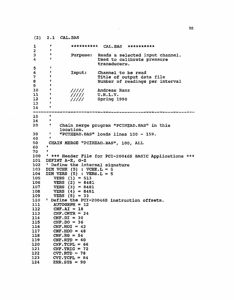
98

(2) 2.1 CAL.BAS12345678910 11 121314

********** CAL.BAS **********Purpose;

Input:

///////////////

Reads a selected input channel. Used to calibrate pressure transducers.Channel to be readTitle of output data fileNumber of readings per intervalAndreas Ranz U.N.L.V.Spring 1990

1516 203040506070100101102103104105106107108109110 111 112113114115116117118119120 121 122123124

Chain merge program "PCIHEAD.BAS" in this location."PCIHEAD.BAS" loads lines 100 - 159.

CHAIN MERGE "PCIHEAD.BAS", 100, ALLI* *** Header File for PCI-20046S BASIC Applications *** DEFINT A-E, G-Z

Define the internal signatureDIM VCHK (5) DIM VERS (5)

VERS (1) VERS VERS VERS VERS

(2)(3)(4)(5)

VCHK.L = 5 VERS.L = 5 513 8481 8481 8481 33

Define the PCI-20046S instruction offsets. AUTOGRPH = 12 CNF.AI = 18 CNF.CNTR = 2 4 CNF.DI = 30 CNF.DO = 36 CNF.HDI = 42 CNF.HDO = 48 CNF.RG = 54 CNF.RTD = 60 CNF.TCPL = 6 6 CNF.TRIG = 7 2 CVT.RTD = 78 CVT.TCPL = 8 4 ERR.SYS = 90

99125 INIT = 96126 READ.CH = 102127 READ.CTS = 108128 READ.FRQ = 114129 READ.SSH = 12 0130 STAT.CNT =126131 STAT.HD = 132132 SYSINIT = 138133 WRITE.CH = 144134 WRITE.GR = 150135 • Define the PCI-20046S I/O types.136 AI = 1137 AO = 2138 CT = 3139 DI = 4140 DIET = 5141 DO = 6142 DOBT = 7143 RG = 8144 TCPL = 9145 TRIG = 10146 RTD = 11147 ' Thermocouple types supported: J K T148 ' RTD ranges supported: 1 2149 '150 DEF SEG = 0 : INTVEC = &H180151 SEGMT = PEEK (INTVEC+2) + &H100*PEEK (INTVEC+3)152 DEF SEG = SEGMT153 ' Check for installed software154 IF (SEGMT <> 0) AND (PEEK (11) = 1) AND (PEEK (12) = &H9A) THEN 156155 PRINT "PCI-20046S not installed or invalid.", CHR$ (7) : END156 CALL AUTOGRPH (VERS.L, VCHK (1), VCHK.L)157 IF (VCHK.L <> VERS.L) THEN 155158 FOR I = 1 TO VCHK.L : IF (VERS (I) <> VCHK (I)) THEN 155159 NEXT I160 180 190 200 210220 DIM ADATA (10)230 DIM FDATA (10)280 '290 •300 ' Set initial values of variables310 '320 FOR I = 1 TO 6 330 '340 ADATA(I) = 0350 FDATA(I) = 0

Dimension variables

100360 COUNTER = 0364 FONT = 0365 DUN = 0366 WTP = 0370 '380 NEXT I 390 '400 '480 '490 GOTO 580 : ' Jump over the error subroutine until needed.500 ' Define the error processing subroutine505 '510 '---- -- Error Subroutine ---530 CALL ERR.SYS (ERROR.CODE)540 IF ERROR.CODE = 0 THEN 560 550 PRINT EROR$ ; ERROR.CODE : END 560 RETURN570 '580 ' -- Error subroutine ---590 '600 '610 '620 ' Initialize the PCI-200462-1 system630 '640 CALL SYSINIT650 '660 '700 ' Define base address of the board710 ' Using &HDOOO — for this application720 '730 HDWSEG = &HDOOO 740 CALL INIT (HDWSEG)750 '760 EROR$ = "ERROR FOUND DURING INIT (LINE 760)"770 GOSUB 500780 '790 810 830 9901000 ' Read and conversion loop1004 •1010 CLS1013 PRINT "Input the title of the data file (.dat); " : INPUT A$1014 OPEN A$ FOR OUTPUT AS #11015 PRINT "Input the channel to be read: " : INPUT CHN1016 PRINT "Input the number of readings: " : INPUT FC1017 PRINT"Input the pressure from DWT: " : INPUT FDWT1018 •1019 DUN = DUN + 11020 COUNTER = COUNTER + 1

I

I

I

I

101102110231024102510391040 1050 1070 1080 1090 1100 1110 1120 1130 1140 1160 51) / 1180 1190 1200 1230 1240 1250 1440 1450 1500 1520 1530 1540 155015551556 1560 1570 1580 1585 1590 1600 PSD 1602 FDWT 1605 1610 162017251726 1870 1880 1900 1910

Begin the data acquisition loop.I IZ.CHN = 0 RANGE = 2 GAIN = 1

CALL CNF.AI (CHN, GAIN, Z.CHN, RANGE)EROR$ = "ERROR FOUND DURING CALL.CNF (LINE 1080)" GOSUB 500

ICALL READ.CH (AI, CHN, ADATA(CHN))EROR$ = "ERROR FOUND DURING READ.CH (LINE 1120)" GOSUB 500I

GAINFDATA(CHN) = ((4095! - ADATA(CHN))*10! / 4096! - IF COUNTER = FC THEN GOTO 1500

' Calculate mean and standard deviationIFSUM = FSUM + FDATA(CHN)FSUM2 = FSUM2 + ( FDATA(CHN) * FDATA(CHN) )GOTO 1020IFMEAN = FSUM / FCFSD = SQR( ( FSUM2 - FMEAN*FMEAN*FC ) / ( FC - 1 ) )

' Write the final data to disk IF DUN <> 1 THEN GOTO 1560 ' OPEN A$ FOR OUTPUT AS #1 WRITE#1, FDWT, FMEAN, FSDt

' Print the data on the screen PRINT "" : PRINT ""PRINT "Mean : " USING "####.######" ; FMEAN PRINT "Standard deviation : " USING "####.######" ;PRINT "Input pressure (DWT) ; " USING "####.######" ;PRINT "" : PRINT "" : SOUND 200,30IICOUNTER = 0 ; DUN = 0FSUM = 0 ; FSUM2 = 0 : FMEAN = 0 : FSD = 0

GOTO 1017ICLOSE #1 END

102

(2)10 20 30 40 50 60 70 80 90 100 110 120 130 140 150 160 170 180 190 200 210 220 230 240 250 • 260 270 280 ' 290 ' 300 ' 310 320 330 ' 340 ' 350 ' 360 ' 370 380 ' 390 400 • 410 430 440 ' 450 460 ' 470 ' 480 ' 490 500 ' 510

2.2 SWITCH.BAS********** SWITCH.BAS **********Purpose: Switch the columns in the data

files used for calibrating the pressure transducers.

Input: Data files CAL_.DAT with columns'y', 'X', 'z'.

Output: Data files CAL_.DAT with columns•x' , 'y', 'z *.

///// Andreas Ranz///// U.N.L.V.///// Summer 1990

This section opens the input and output files CLSINPUT "Input the input data file: ", 1$PRINT ""INPUT "Input the output data file: ", 0$

OPEN 1$ FOR INPUT AS #1 OPEN 0$ FOR OUTPUT AS #2Dimension arraysLET D = 100DIM X(D) : DIM Y(D) : DIM Z(D)

This section reads in the fileLET 1 = 1WHILE NOT EOF(l)

INPUT #1, Y (I), X(I), Z(I)LET 1 = 1 + 1

WENDThis section writes the new columns to a file FOR N = 1 TO I-l

PRINT #2, X(N), Y(N), Z(N)

520 ■530 NEXT N 540 '550 ' This section closes the open files 560 '570 CLOSE #1 : CLOSE #2580 '590 END

104

(2)1020304060708090100110120130140150160170

2.3 NTHORDER.BAS * * * * * * * * * * NTHORDER.BAS **********Purpose: Read in a set of x(i) and y(i) data

pairs.Choose the order of the polynominal in the least squares scheme.Generate a system of N equations in the form:y = ao + al*x + a2*x^2 + ... + an*x^n Later, a matrix inversion scheme will be used to solve for the coeffecients.

Input: A data file with x,y pairsThe order of the polynominal to use

///// Andreas Ranz///// U.N.L.V.///// Summer 1990

180190 ' Dimension the variables. Set dimension size in the

program.200 '210 LET DIMENSIONSIZE = 100220 DIM X(DIMENSIONSIZE) : DIM Y (DIMENSIONSIZE) : DIMB(DIMENSIONSIZE)230 DIM A(DIMENSIONSIZE,DIMENSIONSIZE) : DIMZ(DIMENSIONSIZE)240 •250 ' Set variables to zero prior to entering calculations260 '270 280 290 300 310 320330 CLS : PRINT "Input the data.dat file to use asinput: " : INPUT D$340 OPEN D$ FOR INPUT AS #1350 '360 '370 •380 PRINT "" : PRINT "Input the number of data pairs: ": INPUT M385 PRINT "" : PRINT "Input the order of thepolynominal: " : INPUT N 390 '

FOR I = 0 TO DIMENSIONSIZE X(I) = 0:Y(I) = 0:B(I) = 0

NEXT I' Loop 1 (i) ' Loop 1 (i)

Read in the data.dat file to use as input

Read in the number of data pairs and the data

105400 FOR I = 1 TO M : ' Loop 2 (i) ----------405 '410 INPUT #1, X(I), Y(I), Z(I) : ' Calibration datafile has 3411 ' variables in a data pair415 ' variables in a row420 NEXT I : ' Loop 2 (i) -----------430 '500 ' Start the calculation loops510 '520 FOR J = 0 TO N : ' Loop 3 (j) !!!!!!!!!!530 '540 FOR K = 0 TO N : ' Loop 4 (k) **********550 '560 FOR I = 1 TO M : ' Loop 5 (i) ----------570 •580 LET A(K,J) = A(K,J) + (X(I))^(J+K)585 '590 NEXT I : ' Loop 5 (i) ----------600 '610 NEXT K : ' Loop 4 (k) **********620 '630 NEXT J ; ' Loop 3 (j) ! ! 1 ! ! ! ! 1 ! !640 '650 '660 FOR J = 0 TO N : ' Loop 6 (j) %%%%%%%%%%670 '680 FOR I = 1 TO M : ' Loop 7 (i) )))))))))690 '700 LET B(J) = B(J) + Y(I) * ( X(I) J )710 '720 NEXT I : ' Loop 7 (i) ))))))))))730 '740 NEXT J : • Loop 6 (j) %%%%%%%%%%750 '760 ' Close the input data file770 '780 CLOSE #1790 '900 • This section prepares the coeffecients of the equations910 ' to be read in by a program which solves N equations and920 ' N unknowns. The output is the coeffecients of the930 ' Nth order polynominal; ao,al,a2,...,an940 '950 ' Open an output data file960 '970 PRINT "" ; PRINT "Input the output data file to be used: " : INPUT 0$980 OPEN 0$ FOR OUTPUT AS #2990 •

1061000 ' Print to the data file1010 '1020 LET NEQNS = N + 11030 PRINT #2, NEQNS1040 '1050 FOR J = 0 TO N I1060 '1070 FOR K = 0 TO N1080 '1090 PRINT #2, A(K,J)1100 '1110 NEXT K1120 '1130 PRINT #2, B(J)1140 •1150 NEXT J :1160 '1170 ' Close output data file1180 '1190 CLOSE #21200 •9999 END

: ' Loop 8 (k) I 1 !!!!!!! !

; ' Loop 8 (k) !!!!!!!!!!

107

(2) 2.4 MATRIXIN.BAS10 ' ********** MATRIXIN.BAS **********20 '30 ' Purpose: This program allows the student to input a40 ' matrix to a set of simultaneous equations

to be solved and allows them to store these values on disk. The matrix is stored in a file with the suffix "mat".

70 ' Up to 100 simultaneous equations can behandled.

80 '90 ' Input: i) Update an old matrix file100 ' ii) Enter matrix file by keyboard110 ' iii) Enter matrix file from data file120 '130 ' ///// Original Author: Dr. William Culbreth140 ' ///// Updated by: Andreas Ranz150 ' ///// U.N.L.V.160 ' ///// Summer 1990170 '180I ______190 '200 DIM 0(100,100)210 I220 ' 1. Ask initial questions.230 '240 CLS250 PRINT "********************************************"260 PRINT "* MATRIXIN — MATRIX INPUT PROGRAM *"270 PRINT "********************************************"280 PRINT290 PRINT "A. Please answer questions with (yes/no)."300 PRINT310 INPUT "B. Do you wish to update an old matrix file?", UPDATE$320 PRINT330 IF LEFT$(UPDATE$,l)="n" OR LEFT$(UPDATE$,1)="N" THENGOTO 410340 PRINT "The following are matrix files on yourdisk: "350 ON ERROR GOTO 410 : FILES "*.MAT"360 INPUT "What is the name of your old matrix file?",FILES370 OPEN FILE$+".MAT" FOR INPUT AS #2380 INPUT #2,NEQNS390 FOR 1=1 TO NEQNS:FOR J=1 TONEQNS+l:INPUT#2,C(I,J):NEXT J:NEXT I400 CLOSE : KILL FILE$+".MAT" : FILE$=""410 ’420 IF FILE$="" THEN INPUT "Input the file your matrix

108will be stored in? ",FILE$430 OPEN FILE$+".MAT" FOR OUTPUT AS #1440 '450 ' 2. Begin the matrix input sequence.460 '470 CLS480 PRINT "************************”490 PRINT "* MATRIX INPUT *"500 PRINT "************************"510 PRINT520 INPUT " 1. Do you want to enter the data bykeyboard? ", BOARDS530 IF LEFTS(BOARDS,l)="n" OR LEFTS(BOARDS,1)="N" THENGOTO 1180540 INPUT " 2. How many equations are to be solved?(size of matrix)=",NEQNS550 PRINT " 3. The coefficients of the matrix cannow be entered."560 PRINT " These coefficients will be asked forin order as:"570 PRINT580 PRINT " coefficient(row, column)"590 PRINT600 PRINT " 4. If you make a mistake, wait until alldata has been"610 PRINT " entered. You will then be given achance to make"620 PRINT " corrections."630 PRINT " 5. If you do not wish to change thedefault value of any"640 PRINT " coefficient, simply hit the returnkey. "650 PRINT660 PRINT " 6. Hit the return key to continue on."670 INPUT HOLD.ON680 CLS690 '700 ' 3. Ask the student for the contents of the matrix.710 •720 FOR IR0W=1 TO NEQNS730 FOR IC0L=1 TO NEQNS+1740 PRINT "c(";IROW;",";ICOL;") = ";C(IROW,ICOL)750 INPUT " New value = ",NEWVALS760 IF VAL(NEWVALS)=0 AND NEWVAL$<>"" THENC(IROW,ICOL)=0770 IF NEWVALSo "" THEN C (IROW, ICOL) =VAL(NEWVALS)780 NEXT ICOL790 NEXT IROW800 '810 ' 4. Store the matrix on disk.820 '830 ' a. Give the student a chance to makecorrections, first.

109840 '850 GOSUB 1010860 PRINT#1,NEQNS870 FOR 1=1 TO NEQNS 880 FOR J=1 TO NEQNS+1890 PRINT#1,C(I,J)900 PRINT " c(";I;",";J;") = ",C(I,J)910 NEXT J920 NEXT I930 CLS940 PRINT "Your data has been written onto disk in a filecalled:"950 PRINT960 PRINT " ";FILE$+".MAT"970 PRINT980 PRINT "The program ends here."990 END 1000 '1010 ' Subroutine FIX 1020 '1030 ' PURPOSE: This subroutine allows the student to fixa data point1040 ' already entered.1050 '1060 PRINT "" : PRINT"This section allows the user tofix or see any data point entered." ; PRINT ""1070 PRINT "Which point do you want to fix or see?c (row , column)."1080 PRINT " (enter * to stop editing and write yourdata to disk)"1090 INPUT " Row = ", STARS1100 IF STARS="*" t h e n g ot o 1170 ELSE IROW=VAL(STARS)1110 INPUT " column = ",ICOL1120 PRINT " c(";IROW;",";ICOL;") =";C(IROW,ICOL)1130 INPUT "What is the new value? ",NEWVALS1140 IF VAL (NEWVALS )=0 AND NEWVALS<>'"' THENC(IROW,ICOL)=01150 IF NEWVALSo "" THEN C(IROW, ICOL) =VAL(NEWVALS)1160 GOTO 10601170 RETURN 1180 '1190 ' 5. Asking for input data from a data file and notfrom1200 ' keyboard input.1210 ' This section is acting as a subroutine when theinput1220 • required is in a data file (.dat).1230 '1240 PRINT ""1250 INPUT " 2. Input the name of the data file touse: ", DATAFILES1260 OPEN DATAFILES+".DAT" FOR INPUT AS #2

1101270 '1280 INPUT #2, NEQNS 1290 '1300 '1310 FOR IROW = 1 TO NEQNS : ' Loop 1 (irow)1320 FOR ICOL = 1 TO NEQNS + 1 : ' Loop 2 (icol)* * * * * * * * * * * <1330 '1340 INPUT #2, NEWVALS1350 IF VAL(NEWVALS) = 0 AND NEWVALS<>"" THENC(IROW,ICOL) = 01360 IF NEWVALSo"" THEN C(IROW,ICOL) = VAL (NEWVALS)1370 •1380 NEXT ICOL ; • Loop 2 (icol)* * * * * * * * * *1390 NEXT IROW ; ' Loop 1 (irow)1400 '1410 ' Return to the main program beneath the input section for1420 ' the keyboard 1430 '1440 GOTO 810 1450 '1460 END

I OOP•auTC^noaqns aAlOS aqq. dn tt^O *Z , 06CI 08C

T# aSOIO O L ZI iX3N:r ixaN : (f'i)o'T#andNi

: T+SNÔ3N OJ, T=f HOd : SN03N 01 T=I HOd 09 CSN03N = SMOHN OSESND3N'T#indNI OfrE

I oeeT# SV indNI HOd iilVW* ii+$33Id N3d0 OEE

$33Id ' .1ipaATOs quew noA op atxj xTaqaut qaiiM *a„ indNI OTEINIHd 00Ei.qaui'*,, sanid 06EINIHd 08E„:3{STp anoA

uo punoj aaam saixj xxaq.aui Bu x m o x t oJ aqi 'Yu INIHd OZ.ZINiad 09EINIHd OSE

H*wvaooad NOISaaANI XIHIYW — 1H3ANI *„ INIHd OtEINIHd OEE

S30 OEEI OTE•uaaaos aqq. dn q.as pus suoxqsanb xexqxux %SY *T , 00EI 061

(00T)d333 ' (OOT'OOT)D Wia 08TI OAT

— — — — — — — — I

09T I OST

066T aauiuins ///// , OPT•A*TN*n ///// I OET

ZUBH saaapuY :Aq paqepdn ///// , OETqqajqino urexiITM ’JQ :aoq:^nY lauxBxao ///// i OTT

1 OOT• ( lYW* :;buuoj aqq. ux ) afrj eqep qndui :qndui , 06• 08

iiSYa-NIXIHlYWii uiaaBoad aqq Aq paaedaad aq u b o puB hIYWii xxjjns aqq aABq pxnoqs axxq aqi , 09

•axTJ Xsxp B jqopBaa aq oq ajB paqaaAux aq oq xxaqBut aqq , os

JO squaxDXjjaoo aqi *uoxqBUTUixxa UBXssnBO JO asn aqq qBnoaqq suoxqanba snoauBqxnuixs

SN03N oq uoxqnxos aqq aqaxnoxBO lasodana , OEI OE

********** SY9*i1H3ANI ********** I OXSY3-IH3ANI S'E (E)

TIT

112410 CLS420 GOSUB 540430 PRINT "The solutions are as follows: "440 FOR 1=1 TO NEQNS: PRINT " X(";I;")=";C(I,NEQNS+1): NEXT I 450 PRINT 460 PRINT 470 INPUT "B.", IWAIT 480 END 490 500 510 520 530 540I__

Please hit <enter> to clear the screen.

550 '560 ' Subroutine SOLVE570 '580 ' PURPOSE: Solve a series of simultaneous equations590 ' through the use of Gaussian elimination. The600 • arguments to this subroutine are:610 '620 ' C(IROW, ICOL) = Coefficients of theequations.630 ' IROW = Equation number, from 1 toNEQNS.640 • ICOL = Number of columns, 1 toNEQNS+1.650 ' NEQNS = Number of equations to besolved.660 '670 • OUTPUT: The solution will appear in C(IR0W=1,NEQNS,NEQNS+1). 680 '690

700 '710 TOLERANCE = .00001720 FOR IR0W=1 TO NROWS 730 OFFSET = 1740 WHILE C(IROW,IROW) < TOLERANCE750 760770 PRINT "here" 780 790 800 810 820

IF (IROWS+OFFSET)I > NROWS THEN GOSUB 1040

FOR IC0L=1 TO (NROWS+1)KEEP(ICOL) = C(IROW,ICOL)C(IROW,ICOL) = C(IROW+OFFSET,ICOL) C(IROW+OFFSET,ICOL) = KEEP(ICOL)

NEXT ICOL

113830 '840 OFFSET = OFFSET+1850 WEND 860 '870 ' 2. Now, normalize the "IROW" equation by its diagnol.880 '890 FOR IC0L=IR0W+1 TO (NROWS+1)900 C(IROW,ICOL) = C(IROW,ICOL)/C(IROW,IROW)910 NEXT ICOL 920 •930 ' 3. Subtract the "IROW" equation from all other equations.940 '950 FOR JR0W=1 TO NROWS960 IF JROW = IROW THEN GOTO 1000970 FOR IC0L=IR0W+1 TO (NROWS+1)980 C(JROW,ICOL) = C(JROW,ICOL) -C(JROW,IROW)*C(IROW,ICOL)990 NEXT ICOL1000 * end if1010 NEXT JROW1020 NEXT IROW 1030 RETURN 1040 '1050 ' Subroutine BADDATA 1060 '1070 ' PURPOSE: This subroutine is called when the1080 ' equations cannot be solved by the method used. 1090 '1100 PRINT "BAD SET OF EQUATIONS, UNSOLVABLE BY THISMETHOD! "1110 RETURN

114

(2) 2.6 CALCLINE.BAS10 ' ********** CALCLINE.BAS **********20 '30 ' This section dimensions the arrays 40 '50 LET D = 5060 DIM DWTPRESSURE(D) : DIM VOLTAGE(D) : DIM SD(D)70 DIM NEWDWTPRESSURE(D) : DIM A(D) : DIM X(D) : DIMDP(D)80 •90 ' This section reads in the old set of x vs y data100 '110 CLS120 INPUT "Input the data file name: ", 1$130 OPEN 1$ FOR INPUT AS #1140 '150 INPUT "Input the number of data pairs: ",NUMPAIRS 160 '170 FOR I = 1 TO NUMPAIRS180 INPUT #1, VOLTAGE(I), DWTPRESSURE(I),SD(I) : ' x, y, : 190 NEXT I200 '210 ' This section determines the calculated value of 220 ' the voltage at each point i.230 ' This program reads in the values of the240 ' coeffecients in a Nth-order approximation scheme.250 '2 60 ' Read in the order of the polynomial.270 '280 INPUT "Input the order of the polynominal: ",NTHORDER290 '300 FOR I = 1 TO (NTHORDER+1)310 PRINT "Input A(";I;")" : INPUT A(I)320 NEXT I330 •340 ' Calculate the newdwtpressure using the coeffecients 350 ' for the polynominal360 '370 FOR I = 1 TO NUMPAIRS380 '390 FOR J = 1 TO (NTHORDER+1)400 '410 NEWDWTPRESSURE(I) = NEWDWTPRESSURE(I) +A(J)*VOLTAGE(I)^(J-1)420 '430 NEXT J440 '450 NEXT I460 '470 ' This section calculates the percent difference

115between480 ' the old value of 'y' and the new value of 'y'.490 '500 FOR I = 1 TO NUMPAIRS 510 '520 DP(I) = ABS(NEWDWTPRESSURE(I) -DWTPRESSURE(I))/DWTPRESSURE(I)530 DP(I) = DP(I) * 100540 '550 NEXT I560 '570 ' This section prints the new values to the screen 580 ' and writes them to an output file.590 '600 ' Determine the output file610 '620 INPUT "Input the name of the output data file; "0$630 OPEN 0$ FOR OUTPUT AS #2640 '650 PRINT "" : PRINT ""660 PRINT " V Dwt P New P

%P Difference"670 PRINT ""680 '690 FOR I = 1 TO NUMPAIRS700 '710 PRINT USING "#######.#######" ; VOLTAGE(I),DWTPRESSURE(I), NEWDWTPRESSURE(I), DP(I)720 PRINT #2, USING "#######.#######" ;VOLTAGE(I),DWTPRESSURE(I), NEWDWTPRESSURE(I), DP(I)730 '740 NEXT I750 •760 • Close all opened files 770 •780 CLOSE #1 : CLOSE #2790 •800 END

116

(2) 2.710 20 30 40 50 60 70 80 90 100 110 120 130 140 150 160 170 180 190 200 210 220 230 240 250 260 270 ' 280 ' 282 ' 290 300 310 ' 320 330 ' 340 350

SERROR.BAS* * * * * * * * * *

Purpose;

Input;///////////////

SERROR.BAS **********Read in 'x ', 'y ', and a 'ynew' calculated by some Nth order approximation. Calculate standard error.Data file with 'x', 'y', and 'ynew'Andreas Ranz U.N.L.V.Summer 1990

This section opens the input and output data filesCLSINPUT "Input the input data file; " , PRINT ""INPUT "Input the output data file; "This section reads in the dataOPEN 1$ FOR INPUT AS #1 OPEN 0$ FOR OUTPUT AS #2

1$0$

Dimension the arrays LET D = 50DIM X(D) ; DIM Y(D) ; DIM YNEW(D) LET 1 = 1

DIM Z(D)

WHILE NOT EOF(l)INPUT #1, X(I), Y(I), YNEW(I), Z(I)

current files 360 'using there are 370 'variables in a data set

' In the we are

390 400 410 ' 420 ' 430 ' 440 450 ' 460 470 '

LET 1 = 1 + 1 WEND

This section calculates the standard error LET N = I - 1 FOR J = 1 TO N

117480 LET DIFF = (Y(J) - YNEW(J))^2490 '500 NEXT J510 '520 LET STANDARDERROR = SQR( 1/N * DIFF )530 '540 ' This section writes the data to a file and to screen 550 •560 PRINT "Voltage","DWT Pressure","New Pressure"570 PRINT #2, "Voltage","DWT Pressure","New Pressure"580 PRINT "" ; PRINT #2, ""590 '600 FOR J = 1 TO N610 '620 PRINT X(J), Y(J), YNEW(J)630 PRINT #2, X(J), Y(J), YNEW(J)640 '650 NEXT J660 '670 PRINT "" : PRINT ""680 PRINT #2, "" : PRINT #2, ""690 '700 PRINT "The standard error is; ", STANDARDERROR710 PRINT #2, "The standard error is; ", STANDARDERROR720 '

118

(3) 3.1 MAIN.BAS

********** MAIN2.BAS **********Purpose; Combine all subroutine programs into

this program. Start with data directly from Control.C and finish with information to calculate the flow coeffecient.Designed for use when calculating the flow gain coefficient, Kq.

///// Andreas Ranz///// U.N.L.V.///// Fall 1990

' SubroutinesSub COMBINE

Input; Data from the test run (Told, Theta, Vs,delta_p_actual, delta_p_desired)

Subroutine; TIMEReturn; Tnew, Theta, Vs, delta_p_actual,

delta_p_desiredSub RADIANS

Input; Theta(i)Internal — Slope, offset

Return; Theta(i) in radians/secSub DIFFER

Input: Tnew, Theta, Vs, delta_p_actual,delta_p_desired

Return; Tnew, Theta, Thetadot, Theta2dotSub VELOCITY

Input: Theta, ThetadotReturn: Theta, Thetadot, Encoder angle. Velocity

(m/s)Sub FLOW

Input: Tnew, Velocity, delta_p_actual, VsReturn: Tnew, delta_p_actual/Ps, Q/Qmax, U/Umax

119DECLARE SUB differentiate (NI, x!(), y!(), Yl!(), Y2l())

' This section dimensions all arrays LET D = 700DIM DELTAPACTUAL(D); DIM DELTAPDESIRED(D)DIM T(D); DIM THETA(D): DIM VOLT(D): DIM OLDTHETA(D)DIM NEWT(D): DIM T1(D): DIM T2(D): DIM OLDT(D); DIM

NEWTl(D)DIM 1(D): DIM x(D): DIM y(D): DIM YCOMPUTED(D)DIM DYDX(D): DIM D2YD2X(D): DIM SERVOVOLTAGE(D)DIM Q(D): DIM DELTAP(D): DIM QQMAX(D): DIM DELTAPPS(D) DIM Y1(D): DIM Y2(D): DIM U(D): DIM UUMAX(D): DIM

THETAR(D)

' Calling subroutines GOSUB COMBINECurrent data: 1) Tnew (seconds starting at 0) -

NEWTl(I)

DELTAPDESIRED(I )

2) Theta (encoder position) - THETA(I)3) Vs (voltage to servovalve) - VOLT(I)4) delta_p_actual (psi) - DELTAPACTUAL(I)5) delta_p_desired (psi) -

GOSUB RADIANS ’ Current data: 1) Theta (rad) - THETA(I)

GOSUB DIFFER ' Current data:I

I

I

1) Tnew (s) - NEWTl(I)2) Theta (rad) - THETA(I)3) Thetadot (rad/s) - Y1(I)4) Theta2dot (rad/s^2) - Y2(I)

GOSUB VELOCITYCurrent data:

GOSUB FLOW

1) Encoder angle (rad) - PHIl(I)2) Angular velocity (rad/s) - DOTPHIl(I)2) Velocity (in/s) - V2(I)

120

I Current data: 1) Flow rate (in^3/s) - Q(I)

DELTAPACTUALPS(I)I

2) delta_p_actual (psi) - DELTAPACTUAL(I)3) (Q / Qmax) - QQMAX(I)4) delta_p_actual / Ps -5) (U / Umax) - UUMAX(I)

' This section outputs the data to disk file CLSINPUT "The output file name: ", 0$

' Output to diskOPEN 0$ FOR OUTPUT AS #2

' PRINT #2, " Tnew Theta DPa/PsQ/Qmax U/Umax"' PRINT #2, PRINT #2, ""

FOR I = 1 TO NITEMSPRINT #2, USING "####.##"; NEWTl(I), THETA(I),

DELTAPPS(I), QQMAX(I), UUMAX(I)NEXT I

' PRINT #2, "": PRINT #2, ""' PRINT #2, " The desired pressure was: ",DELTAPDESIRED(1)' Output to screen

PRINT " Tnew Theta DPa/PsQ/Qmax U/Umax"

PRINT "": PRINT ""FOR I = 1 TO NITEMS

PRINT USING " # # # # . nEWTI(I), THETA (I) , DELTAPPS(I), QQMAX(I), UUMAX(I)

NEXT IPRINT "": PRINT ""PRINT " The desired pressure was: ", DELTAPDESIRED(1)CLOSEEND

COMBINE:

El

121This section reads in the input and output data files CLS ; PRINTINPUT "Input the input data file: ", 1$This section opens the fileOPEN 1$ FOR INPUT AS #1

This section reads in the valuesLET 1 = 1 WHILE NOT EOF(l)

INPUT #1, T(I), THETA(I), DELTAPACTUAL(I), VOLT(I),LET 1 = 1 + 1

WENDLET N = I - 1: • N is the number of pairs of dataLET NITEMS = NINPUT "Delta P desired was;", DELTAPDESIRED(1)

' This section calls the subroutines GOSUB TIME

RETURN' Returning to MAIN programTIME:' Set starting values for loop - l

LET 1 = 1LET FIRSTT = T(I)LET T1(I) = OLDT(I)LET T2(I) = T(I)

' Start loop - 2 which convertsLET 1 = 1

HEREl: IF (T2(I) - T1(I)) < 0 THEN NEWT(I) = 60 -ABS(T2(I) - T1(I)) + NEWT(I)

IF (T2(I) - T1(I)) < 0 THEN GOTO HERE2LET NEWT(I) = NEWT(I) + (T2(I) - T1(I))

HERE2: OLDT(I) = T(I)LET NEWTl(I) = NEWT(I) - FIRSTT

172IF NEWTl(I) < 0 THEN NEWTl(I) = 60 - ABS(NEWTl(I))IF I = N THEN GOTO HERE31 = 1 + 1LET T1(I) = T2(I)LET T2(I) = T(I)GOTO HEREl

HERE3: •RETURN

' Returning to subroutine COMBINERADIANS ;' This section sets the constants

LET OFFSET = 765!LET PI = 3.1415927#FOR I = 1 TO NITEMS

GAP = THETA(I) - OFFSETIF GAP < 0! THEN THETAR(I) = (THETA(I) - OFFSET) * 2 *

PI / 16384!' In this configuration the range of theta is 0 to3.14159 for' quadrants 1 and 2, 0 to -3.14159 radians forquadrants 3 and 4.' The 0 reference angle is at 3:00.' If the range of theta should be between 0 and6.26318 radians' then add to the end of the above line: ( + 2 * PI ).

IF GAP >= 0! THEN THETAR(I) = (THETA(I) - OFFSET) * 2 * PI / 16384!

OLDTHETA(I) = THETA(I): ' OLDTHETA(I) is in encoder position values

THETA(I) = THETAR(I): ' THETA(I) is in rad/sNEXT IRETURN

' Returning to MAIN program

DIFFER:

I

123CLSThis section inputs the dataFOR I = 1 TO NITEMS; ' NITEMS taken from inital read in

of RUN_.DATx(I) = NEWT(I): ' Data taken from returning COMBINE

- NEWT(I)y (I) = THETA(I); ' Data taken from returning RADIANS

- THETA(I)NEXT I

' This section calls 'differentiate'CALL differentiate(NITEMS, x(), y(), Yl(), Y2())

' Plot out the resulting curves if desired.PRINT ""PRINT "Would you like the curves of encoder position

vs the"INPUT "first and second derivatives printed to the

screen? ", ANSWER$IF ANSWER$ = "n" THEN GOTO NOPRINTSCREEN 9 ; CLSx.min = x(l); x.max = x(l) y.min = y(l); y.max = y(l) yl.min = Yl(l): yl.max = Yl(l) y2.min = Y2(l); y2.max = Y2(l)

FOR I = 1 TO NITEMSIF X.min > x(I) THEN x.min = x(I)IF x.max < x(I) THEN x.max = x(I)IF y.min > y(I) THEN y.min = y (I)IF y.max < y(I) THEN y.max = y (I)IF yl.min > Y1(I) THEN yl.min = Y1(I)IF yl.max < Y1(I) THEN yl.max = Y1(I)IF y2.min > Y2(I) THEN y2.min = Y2(I)IF y2.max < Y2(I) THEN y2.max = Y2(I)

NEXT IWINDOW (x.min, y.min)“ (x.max, y.max)

PSET (x(l), y(l))FOR I = 1 TO NITEMS

LINE “ (X(I), y(I)), 1LOCATE 2, 1PRINT I, X(I), y (I)

NEXT I

124WINDOW (x.min, yl.min)- (x.max, yl.max)PSET (x(l), Y1(I))

FOR I = 1 TO NITEMSLINE -(X(I), Y1(I)), 2LOCATE 3, 1PRINT I, X ( I ), Y1(I)

NEXT IWINDOW (x.min, y2.min)-(x.max, y2.max)PSET (x(l), Y2(I))

FOR I = 1 TO NITEMSLINE -(X(I), Y2(I)), 3LOCATE 4, 1PRINT I, X ( I ), Y2(I)

NEXT IHIT:

INPUT "Hit any key to continue: ", dum$IF dum$ = "" THEN PRINT "Except that one.": GOTO HIT

NOPRINT: ' Decided not to print curves to screen.

RETURN' Returning to MAIN program

VELOCITY:

' This section sets the constant valuest

PIB = .235: ' In metersYAl = .546: ' In metersXA = .187: ' In meters

' This section dimensions arraysI

LET E = 700DIM PHIl(E): DIM V2(E): DIM DOTPHIl(E)

' This section reads in the encoder angle and angular velocityI

CLSPRINT ""INPUT "Is this single input data ( 'y' or 'n'): ", ANS$ IF ANS$ = "y" THEN GOTO YESN = NITEMS; ' Number of data pairs from initial read inGOTO CALCULATION; ' Skipping section SINGLE which is

used for single input data

125

YES:N = NITEMSINPUT "Input the encoder angle: ", PHIl1 = 1 N = 1LET PHIl(I) = PHIl: • Needed when using single

input dataCALCULATION:' Starting calculations' Changing variable assignments here to use current values

FOR I = 1 TO NPHI1(I) = THETA(I): ' Theta(I) from RADIANSDOTPHIl(I) = Y1(I): ' Angular velocity ( thetadot(I)

NEXT IThis section calculates the velocity FOR I = 1 TO N

A1 = (SIN(PHI1(I)) * PIB + YAl) 2 A2 = (PIB * COS(PHIl(I)) - XA) 2 PAB = (A1 + A2) .5B1 = PIB * (YAl * COS(PHIl(I)) + XA * SIN(PHIl(I))) *

DOTPHIl(I)V2(I) = B1 / PABV2(I) =V2(I) *39.37: ' Convert velocity from meters

to inchesNEXT IRETURN

' Returning to MAIN program FLOW:

N = NITEMS: ' The number of data pairs from COMBINE FOR I = 1 TO N

DYDX(I) = V2(I): ' V2(I) is in (in/s) fromVELOCITY

NEXT I' This section sets up the values for the constantsI

LET PI = 3.1415927#:LET DIAMETER = 1i:

of the actuator shaft (in)LET A = DIAMETER 2 * PI / 4:

area for the servovalve (in)LET QMAX = 96.2497:

rate for the servovalve (in^3.s)LET PS = 800!:

pressure (psi) for the actuators

126Pi constant DIAMETER = diameterA = cross-sectionalQMAX = maximum flowPS = reference

' This section calculates Q(j), DELTAP(j), QQMAX(j), DELTAPPS(j)

LET J = 0 FOR J = 1 TO N

Q(J) = DYDX(J) * ADELTAP(J) = DELTAPACTUAL(J): • used to be P3(J) -

P4(J)QQMAX(J) = Q(J) / QMAX DELTAPPS(J) = DELTAP(J) / PS

NEXT J' This section calculates U/Umax

UMAX =5!; ' Maximum voltage to servovalve (volts)FOR I = 1 TO NITEMS

U(I) = VOLT(I)UUMAX(I) = U(I) / UMAX

NEXT IRETURN

' Returning to MAIN programSUB differentiate (N, x(), y(), Yl(), Y2())

' Compute the first and second derivatives of the data x,y. IF N < 7 THEN PRINT "I need more points!!!" delta.X = (x(N) - x(l)) / N

1, Compute the first derivatives.factor = (1! / (60! * delta.x))

Yl(l) = factor * (-147 * y(l) + 360 * y (2) - 450 * y(3) +

127400 * y(4) - 225 * y(5) + 72 * y(6) - 10 * y(7))

Yl(2) = factor * (-147 * y(2) + 360 * y(3) - 450 * y(4) +400 * y(5) - 225 * y(6) + 72 * y(7) - 10 * y(8))

Yl(3) = factor * (-147 * y(3) + 360 * y(4) - 450 * y (5) +400 * y(6) - 225 * y(7) + 72 * y(8) - 10 * y(9))

Y1(N - 0) = factor * (10 * y(N - 6) - 72 * y(N - 5) + 225* y(N - 4) - 400 * y(N - 3) + 450 * y(N - 2) - 360 * y(N -1) + 147 * y(N - 0))

Y1(N - 1) = factor * (10 * y(N - 7) - 72 * y(N - 6) + 225* y(N - 5) - 400 * y(N - 4) + 450 * y(N - 3) - 360 * y(N -2) + 147 * y(N - 1))

Y1(N - 2) - factor * (10 * y(N - 8) - 72 * y(N - 7) + 225* y(N - 6) - 400 * y(N - 5) + 450 * y(N - 4) - 360 * y(N -3) + 147 * y(N - 2))

FOR I = 4 TO (N - 3)Y1(I) = factor * (-1 * y (I - 3) + 9 * y (I - 2) - 45 *

y(I - 1) + 0 * y(I) + 45 * y(I +1) - 9 * y(I + 2) + 1 * y(I + 3))

NEXT I' 2. Compute the second derivatives.

factor = (1! / (180! * delta.x * delta.x))Y2(l) = factor * (812 * y(l) - 3132 * y(2) + 5265 * y(3)

- 5080 * y(4) + 2970 * y (5) - 972 * y(6) + 137 * y(7))Y2(2) = factor * (812 * y(2) - 3132 * y(3) + 5265 * y ( 4 )

- 5080 * y(5) + 2970 * y(6) - 972 * y(7) + 137 * y(8))Y2(3) = factor * (812 * y(3) - 3132 * y(4) + 5265 * y(5)

- 5080 * y(6) + 2970 * y(7) - 972 * y(8) + 137 * y(9))Y2(N - 0) = factor * (10 * y(N - 6) - 72 * y (N - 5) + 225

* y(N - 4) - 400 * y(N - 3) + 450 * y(N - 2) - 360 * y (N -1) + 147 * y(N - 0))

Y2(N - 1) = factor * (10 * y(N - 7) - 72 * y(N - 6) + 225* y(N - 5) - 400 * y(N - 4) + 450 * y(N - 3) - 360 * y (N -2) + 147 * y(N - 1))

Y2(N - 2) = factor * (10 * y(N - 8) - 72 * y (N - 7) + 225* y(N - 6) - 400 * y(N - 5) + 450 * y(N - 4) - 360 * y(N -3) + 147 * y(N - 2))

FOR I = 4 TO (N - 3)Y 2 ( I ) = factor * (2 * y ( I - 3) - 2 7 * y (I - 2) + 2 7 0 *

y ( I - 1) - 4 9 0 * y ( I ) + 2 7 0 * y ( I + 1 ) - 2 7 * y ( I + 2 ) + 2 *y ( I + 3))

NEXT IEND SUB

128

( 3 ) 3 . 2 SEMOD.BAS10 1 ********** SEMOD.BAS **********20 130 1 Purpose: Read in a data file. Assuming astraight4 0 f line profile and using the leastsquares50 1 method calculate the coeffecients mand b in60 1 the equation — y = mx + b70 1 Also, calculate the standard error80 t90 f Input: N - the number of data pairs1 0 0 t DATA.DAT file to read1 1 0 1 The name of the output DATA.DAT file1 2 0 11 3 0 1 ///// Andreas Ranz140 1 ///// U.N.L.V.1 5 0 I ///// Spring 1 9 9 01 6 0 11 7 0 1

1 8 0 f1 9 0 f Input section2 0 0 12 0 5 PRINT "" : PRINT ""2 1 0 1 PRINT "Input the number of data pairs: ( 3 1 )

INPUT N2201$2300$240 •250 260 270 280 290295296297298299

PRINT "Input the DATA.DAT file to read:"; PRINT "Input the DATA.DAT output file:":

OPEN 1$ FOR INPUT AS #1 OPEN 0$ FOR OUTPUT AS #2

INPUTINPUT

300YY(N)305

Dimension arrays and set values to zeroLET XI = Y1 = X12 = XY = X2 = 0 LET B = B1 = B2 = 0 LET M = Ml = M2 = 0 LET SE = YHl = 0LET N = 1000DIM X(N): DIM Y(N): DIM Z(N): DIM YHAT(N) DIMDIM DY(N)

LET 1 = 1 WHILE NOT EOF(l)

129

INPUT #1, DUMl, DUM2, DUM3, Y(I), X(I)LET 1 = 1 + 1

WEND' Variable assignment for reading the file created byMain2.bas

Duml - dummy variable for T Dum2 - dummy variable for theta Dum3 - dummy varaible for delta P / Ps Y (I) - Q/Qmax X(I) - U/Umax

LET N = I - 1: ' N is the number of pairs of data

Read in data pairsFOR I = 1 TO N INPUT #1, Y(I), X(I), Z(I) y(i) - pressure in the data file x(i) - voltage in the data file

NEXT I

310320330340350355356 360 370380 390 400 410 •420 430 440(X(I))^2 450 Y(I)470 '480 490 '495X(I))^2496 '500 510 520 530 '540 550 560 570 •580 'calculated pressure

Calculations for m and b FOR I = 1 TO N

LET XI = XI + X(I): 'LET Y1 = Y1 + Y(I); 'LET X12 = X12 + (X(I) * X(I))

SUM OF X(I) SUM OF Y (I) ' SUM OF

LET XY = (X(I) * Y(I)) + XY: ' SUM OF X(I) *

NEXT ILET X2 = XI * XI: ' (SUM OF

LET B1 = (Y1 * X12) - (XI * XY)LET B2 = (N * X12) - X2LET B = B1 / B2: ' BLET Ml = (N * XY) - (Y1 * XI)LET M2 = (N * X12) - X2LET M = Ml / M2: ' M

Calculations for standard deviation and

130590 '600 FOR I = 1 TO N610 '620 LET YHAT(I) = (M * X(I)) + B630 LET YHl = (Y(I) - YHAT(I)) 2635 LET YY(I) = M * X(I) + B636 LET DY(I) = ABS(YY(I) - Y(I))640 '650 NEXT I660 '670 LET SE = SQR((1 / N) * YHl): ' SE680 '690 ' Output to DATA.DAT file700 •710 '720 725 730 740 750 755 760 770 780 790 800810 820 830 840 '850 PRINT #2, X(I), Y(I), YY(I), DY(I)860 •870 NEXT I' Output to screen

PRINT ""PRINT "Voltage Pressure New

Pressure Difference"PRINT ""FOR I = 1 TO N

PRINT X(I), Y(I), YY(I), DY(I)NEXT IPRINT ""PRINT "This is output from SE.BAS"PRINT "The input file was: ", 1$PRINT "The output file is: ", 0$PRINT ""PRINT "For the equation — y == mx + b"PRINT ""PRINT "Value for m:", M

PRINT # 2 , "This is output from SEMOD.BAS"PRINT # 2 , "The input file was: ", 1$PRINT # 2 , "The output file is: ", 0$PRINT # 2 , II II

PRINT # 2 , "For the equation — y = mx + b"PRINT # 2 , I I I I

PRINT # 2 , "Value for m:", MPRINT # 2 , "Value for b:", BPRINT # 2 , "Value for standard error:", SEPRINT # 2 , II II

PRINT # 2 , "Voltage Pressure NewPressure Difference"

PRINT1

# 2 , If II

FOR I = 1 TO N

131PRINT "Value for b:", BPRINT "Value for standard error:", SEPRINT ""

880 '890 ' Close files900 '910 CLOSE #1920 CLOSE #2930 ’999 END

132

APPENDIX B — Tables and Graphs of Results

Section 1; Data Tables of Results Section 2; Graphs of Results

133

Section 1; Data Tables of Results

l.A) Raw Data used for Calibrating the Pressure Transducers1) File containing the raw data used for

calibration of pressure transducer 3.2) File containing the raw data used for

calibration of pressure transducer 4.l.B) Calibration of Pressure Transducer 3.

1) INVERT.BAS output2) SERROR.BAS output

(i) Serror31.dat(ii) Serror32.dat(iii) Serror33.dat(iv) Serror34.dat

3) PERSD.BAS outputl.C) Calibration of Pressure Transducer 4.

1) INVERT.BAS output2) SERROR.BAS output

(i) Serror41.dat(ii) Serror42.dat(iii) Serror43.dat(iv) Serror4 4.dat

3) PERSD.BAS outputl.D) Flow Pressure Coefficient, K., Equation Data

1) Test runs for:(i) Upward motion(ii) Downward motion

l.E) Flow Gain Coefficient, K , Equation Data1) Test runs for;

(i) Upward motion(ii) Downward motion

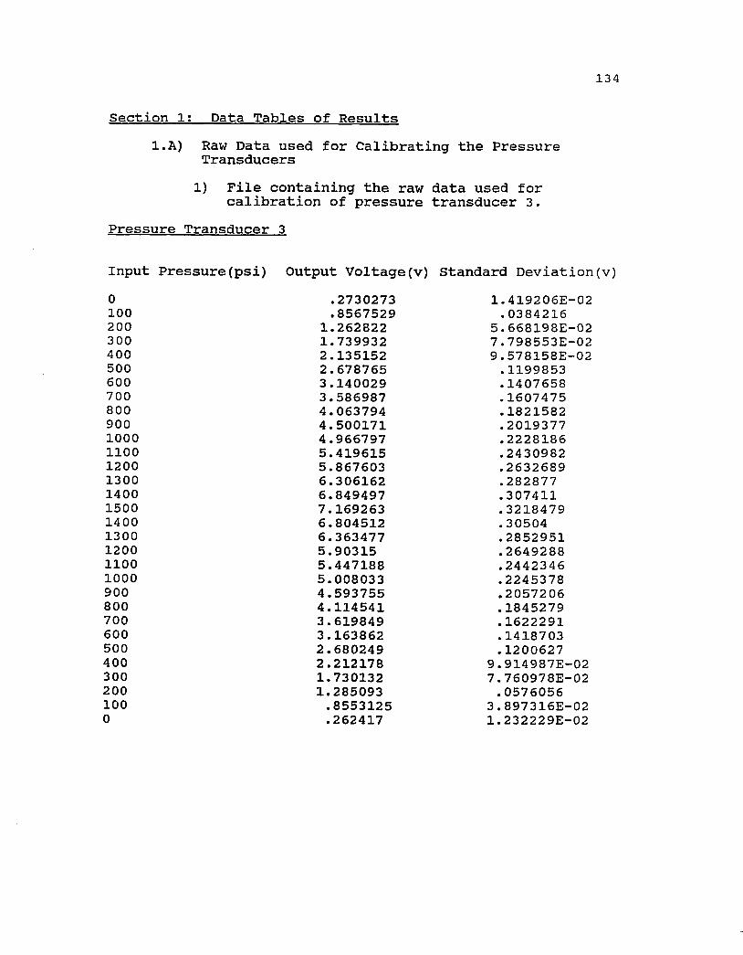
134

Section 1: Data Tables of Resultsl.A) Raw Data used for Calibrating the Pressure

Transducers1) File containing the raw data used for

calibration of pressure transducer 3.Pressure Transducer 3

Input Pressure(psi) Output Voltage(v) Standard Deviation0 .2730273 1.419206E-02100 .8567529 . 0384216200 1.262822 5.668198E-02300 1.739932 7.798553E-02400 2.135152 9.578158E-02500 2.678765 .1199853600 3.140029 .1407658700 3.586987 .1607475800 4.063794 .1821582900 4.500171 .20193771000 4.966797 .22281861100 5.419615 .24309821200 5.867603 .26326891300 6.306162 .2828771400 6.849497 .3074111500 7.169263 . 32184791400 6.804512 .305041300 6.363477 .28529511200 5.90315 .26492881100 5.447188 .24423461000 5.008033 .2245378900 4.593755 .2057206800 4.114541 .1845279700 3.619849 .1622291600 3.163862 .1418703500 2.680249 .1200627400 2.212178 9.914987E-02300 1.730132 7.760978E-02200 1.285093 .0576056100 .8553125 3.897316E-020 .262417 1.232229E-02

135

Section 1: Data Tables of Resultsl.A) Raw Data used for Calibrating the Pressure

Transducers2) File containing the raw data used for

calibration of pressure transducer 4.Pressure Transducer 4

Input Pressure(psi) Output Voltage(v) Standard Deviatio0 .2240576 1.019646E-02100 .7736133 3.474284E-02200 1.234502 5.533453E-02300 1.662241 7.446821E-02400 2.190293 9.811312E-02500 2.580068 .1156308600 3.110073 .1392211700 3.534429 .1583279800 4.004907 .1793376900 4.492627 .20138941000 4.886514 .21911651100 5.322183 .23858421200 5.959517 .26713571300 6.436983 .28871131400 6.759668 .30332211500 7.178472 .32179321400 6.732124 .30182811300 6.220088 .27894081200 5.837618 .26155361100 5.441914 .24383771000 4.924609 .2204655900 4.454107 .1995394800 4.05897 .1817871700 3.541377 .1587692600 3.089116 .1386436500 2.630181 .1180118400 2.152691 9.654982E-02300 1.680557 7.528174E-02200 1.229863 5.517293E-02100 .7756885 3.479649E-020 .3476221 1.564163E-02

136

Section 1: Data Tables of Resultsl.B) Calibration of Pressure Transducer 3.

1) INVERT.BASThe values x(n) are the coefficients for the equations

used to calculate the new pressures(psi) from the voltage measurements of the DWT.

1) Inverts1:

2) Inverts2:

3) Inverts3;

x(l) = -76.164(V) x(2) = 216.446(v) standard error = 3.478(v)x(l) = -63.256(v) x(2) = 206.2061(v) x(3) = 1.390(v)standard error = 1.625(v)x(l) = -63.785(v) x(2) = 207.016(v) x(3) = 1.118(v)x(4) = 2.462(V)standard error = 1.684(v)

4) Inverts4: x(l) = -57.230(v) x(2) = 190.592(V)X(3) = 10.973(V)x(4) = -2.051(v)x(5) = 0.141(v)standard error = l.l66(v)

137

Section 1; Data Tables of Resultsl.B) Calibration of Pressure Transducer 3

2) SERROR.BAS output(i) Serror31.dat

Voltage DWT Pressure(psi) New Pressure(psi).2730273 0 -17.06854.8567529 100 109.27691.262822 200 197.16921.739932 300 300.4382.135152 400 385.9822.678765 500 503.64523.140029 600 603.48423.586987 700 700.22684.063794 800 803.43014.500171 900 897.88244.966797 1000 998.88195.419615 1100 1096.8935.867603 1200 1193.8586.306162 1300 1288.7836.849497 1400 1406.3867.169263 1500 1475.5986.804512 1400 1396.6496.363477 1300 1301.1895.90315 1200 1201.5525.447188 1100 1102.8615.008033 1000 1007.8074.593755 900 918.13824.114541 800 814.4143.619849 700 707.33963.163862 600 608.64282.680249 500 503.96642.212178 400 402.6541.730132 300 298.31681.285093 200 201.9896.8553125 100 108.9651.262417 0 -19.36511

The standard error is; 3.478077(psi)This is output from; SERROR.BASThis is data file; serror31.datThe input data came from data file; calc31.dat

138

Section It Data Tables of Resultsl.B) Calibration of Pressure Transducer 3,

2) SERROR.BAS output(ii) Serror32.dat

Voltage DWT Pressure(psi) New Pressure(psi).2730273 0 -6.852886.8567529 100 114.43171.262822 200 199.36211.739932 300 299.73662.135152 400 383.36252.678765 500 499.09673.140029 600 597.94333.586987 700 694.28844.063794 800 797.68014.500171 900 892.85894.966797 1000 995.2215.419615 1100 1095.1335.867603 1200 1194.546.306162 1300 1292.3956.849497 1400 1414.3717.169263 1500 1486.546.804512 1400 1404.2416.363477 1300 1305.2245.90315 1200 1202.4525.447188 1100 1101.2355.008033 1000 1004.2964.593755 900 913.33954.114541 800 808.72153.619849 700 701.3943.163862 600 603.06662.680249 500 499.41382.212178 400 399.71121.730132 300 297.66861.285093 200 204.0334.8553125 100 114.1312.262417 0 -9.048696

The standard error is: 1.625194(psi)This is output from: SERROR.BASThis is data file: serror32.datThe input data came from data file: calc32.dat

139

Section 1; Data Tables of Resultsl.B) Calibration of Pressure Transducer 3,

2) SERROR.BAS output(iii) SERROR33

Voltage DWT Pressure(psi) New Pressure(psi).2730273 0 -7.178417.8567529 100 114.41491.262822 200 199.47461.739932 300 299.92662.135152 400 383.56652.678765 500 499.26363.140029 600 598.04343.586987 700 694.30784.063794 800 797.61034.500171 900 892.71844.966797 1000 995.03065.419615 1100 1094.9345.867603 1200 1194.3846.306162 1300 1292.3446.849497 1400 1414.5547.169263 1500 1486.9246.804512 1400 1404.3996.363477 1300 1305.1915.90315 1200 1202.3015.447188 1100 1101.0375.008033 1000 1004.1034.593755 900 913.18644.114541 800 808.64263.619849 700 701.40713.163862 600 603.16282.680249 500 499.58052.212178 400 399.91351.730132 300 297.85761.285093 200 204.1512.8553125 100 114.1139.262417 0 -9.381336

The standard error is: 1.684938(psi)This is output from: SERROR.BASThis is data file: serror33.datThe input data came from data file: calc33.dat

140

Section 1: Data Tables of Resultsl.B) Calibration of Pressure Transducer 3

2) SERROR.BAS output(iv) SERROR34

Voltage DWT Pressure(psi) New Pressure(psi).2730273 0 -4.416982.8567529 100 112.90071.262822 200 197.18181.739932 300 298.0992.135152 400 382.71232.678765 500 499.91723.140029 600 599.67283.586987 700 696.35454.063794 800 799.42584.500171 900 893.75654.966797 1000 994.84045.419615 1100 1093.55.867603 1200 1192.1446.306162 1300 1290.3056.849497 1400 1415.1737.169263 1500 1490.9416.804512 1400 1404.6656.363477 1300 1303.2865.90315 1200 1200.0335.447188 1100 1099.5365.008033 1000 1003.7954.593755 900 914.0024.114541 800 810.3933.619849 700 703.46053.163862 600 604.82882.680249 500 500.23792.212178 400 399.27521.730132 300 296.01071.285093 200 201.8527.8553125 100 112.6051.262417 0 -6.497004

The standard error is: 1.166896(psi)This is output from: SERROR.BASThis is data file: serror34.datThe input data came from data file: calc34.dat

141

Section 1; Data Tables of Resultsl.B) Calibration of Pressure Transducer 3

3) PERSD.BAS outputThis program is PERSD.BAS Input data file: cal3.dat Output data file: persd3.dat Pressure transducer calibrated: 3Date: 6/19/90

Pressure Voltage Stan. Dev. Percent S .D .(psi) (V) (psi)0 0.2730273 0.0141920600 5.1980370000

100 0.8567529000 0.0384216000 4.4845610000200 1.2628220000 0.0566819800 4.4885170000300 1.7399320000 0.0779855300 4.4821030000400 2.1351520000 0.0957815800 4 .4859370000500 2.6787650000 0.1199853000 4.4791280000600 3.1400290000 0.1407658000 4.4829460000700 3.5869870000 0.1607475000 4.4814070000800 4.0637940000 0.1821582000 4.4824660000900 4.5001710000 0.2019377000 4.4873340000

1000 4.9667970000 0.2228186000 4.48616300001100 5.4196150000 0.2430982000 4.48552600001200 5.8676030000 0.2632689000 4.48682200001300 6.3061620000 0.2828770000 4.48572400001400 6.8494970000 0.3074110000 4.48808100001500 7.1692630000 0.3218479000 4.48927500001400 6.8045120000 0.3050400000 4.48290800001300 6.3634770000 0.2852951000 4.48332100001200 5.9031500000 0.2649288000 4.48792200001100 5.4471880000 0.2442346000 4.48368200001000 5.0080330000 0.2245378000 4.4835530000900 4.5937550000 0.2057206000 4.4782670000800 4.1145410000 0.1845279000 4.4847750000700 3.6198490000 0.1622291000 4.4816540000600 3.1638620000 0.1418703000 4.4840870000500 2.6802490000 0.1200627000 4.4795350000400 2.2121780000 0.0991498700 4.4820030000300 1.7301320000 0.0776097800 4.4857720000200 1.2850930000 0.0576056000 4.4826020000100 0.8553125000 0.0389731600 4.5565990000

0 0.2624170000 0.0123222900 4.6956900000

142

Section 1: Data Tables of Resultsl.C) Calibration of Pressure Transducer 4.

1) INVERT.BAS outputThe values x(n) are the coefficients for the equations

used to calculate the new pressures(psi) from the voltage measurements of the DWT.

1) Invert41: x(l) = -66.068 x(2) = 216.346 standard error = 1.641(psi)

2) Invert42: x(l) = -61.634 x(2) = 212.784 X(3) = 0.486standard error = 2.225(psi)

3) Invert43;

4) Invert44:

x(l) = -63.717x(2) = 216.023X(3) = -0.607X(4) = 0.0995standard error = 1.684(psi)x(l)x(2)x(3)x(4)x(5)

-56.816190.59210.973-2.0510.141

standard error = 1.166(psi)

143

Section 1: Data Tables of Resultsl.C) Calibration of Pressure Transducer 4,

2) SERROR.BAS output(i) Serror41.dat

Voltage DWT Pressure(psi) New Pressure(psi).2240576 0 -17.59448.7736133 100 101.31.234502 200 201.01161.662241 300 293.55152.190293 400 407.79372.580068 500 492.12023.110073 600 606.7853.534429 700 698.59284.004907 800 800.37914.492627 900 905.89564.886514 1000 991.11165.322183 1100 1085.3675.959517 1200 1223.2526.436983 1300 1326.556.759668 1400 1396.3627.178472 1500 1486.9696.732124 1400 1390.4036.220088 1300 1279.6265.837618 1200 1196.885.441914 1100 1111.274.924609 1000 999.35324.454107 900 897.56184.05897 800 812.07543.541377 700 700.0963.089116 600 602.2512.630181 500 502.96192.152691 400 399.65861.680557 300 297.51411.229863 200 200.008.7756885 100 101.7489.3476221 0 9.138275

The standard error is; 1.641283(psi)This is output from: SERROR.BASThis is data file: serror41.datThe input data came from data file: calc41.dat

144

Section 1; Data Tables of Resultsl.C) Calibration of Pressure Transducer 4.

2) SERROR.BAS output(ii) Serror42.dat

Voltage DWT Pressure(psi) New Pressure(psi).2240576 0 -13.93722.7736133 100 103.26661.234502 200 201.78711.662241 300 293.40652.190293 400 406.7582.580068 500 490.60123.110073 600 604.8463.534429 700 696.51494.004907 800 798.3524.492627 900 904.14864.886514 1000 989.75995.322183 1100 1084.6285.959517 1200 1223.7436.436983 1300 1328.2226.759668 1400 1398.9577.178472 1500 1490.9146.732124 1400 1392.9156.220088 1300 1280.7345.837618 1200 1197.1055.441914 1100 1110.7334.924609 1000 998.04794.454107 900 895.78444.05897 800 810.0683.541377 700 698.01733.089116 600 600.32352.630181 500 501.39152.152691 400 398.67741.680557 300 297.33371.229863 200 200.7944.7756885 100 103.7097.3476221 0 12.38978

The standard error is: 2.22527(psi)This is output from: SERROR.BASThis is data file: serror42.datThe input data came from data file: calc42.dat

145

Section 1: Data Tables of Resultsl.C) Calibration of Pressure Transducer 4

2) SERROR.BAS output(iii) Serror43.dat

Voltage DWT Pressure(psi) New Pressure(psi).2240576 0 -15.34511.7736133 100 103.0841.234502 200 202.22621.662241 300 294.14572.190293 400 407.57122.580068 500 491.30683.110073 600 605.25473.534429 700 696.6154.004907 800 798.09544.492627 900 903.57124.886514 1000 989.00635.322183 1100 1083.8145.959517 1200 1223.1926.436983 1300 1328.2256.759668 1400 1399.5447.178472 1500 1492.556.732124 1400 1393.4456.220088 1300 1280.4425.837618 1200 1196.4655.441914 1100 1109.9324.924609 1000 997.28264.454107 900 895.22884.05897 800 809.77213.541377 700 698.11193.089116 600 600.74632.630181 500 502.07562.152691 400 399.49451.680557 300 298.08051.229863 200 201.2289.7756885 100 103.5307.3476221 0 11.30791

The standard error is; 2.030961(psi)This is output from: SERROR.BASThis is data file: serror43.datThe input data came from data file: calc43.dat

146

Section 1; Data Tables of Resultsl.C) Calibration of Pressure Transducer 4,

2) SERROR.BAS output(iv) Serror44.dat

Voltage DWT Pressure(psi) New Pressure(psi).2240576 0 -11.78483.7736133 100 101.92971.234502 200 199.88291.662241 300 292.09322.190293 400 406.80692.580068 500 491.65863.110073 600 606.81933.534429 700 698.63814.004907 800 799.96834.492627 900 904.60144.886514 1000 989.00085.322183 1100 1082.5745.959517 1200 1220.866.436983 1300 1326.5896.759668 1400 1399.6477.178472 1500 1497.086.732124 1400 1393.3496.220088 1300 1278.265.837618 1200 1194.2125.441914 1100 1108.3874.924609 1000 997.1684.454107 900 896.34694.05897 800 811.58353.541377 700 700.13813.089116 600 602.27482.630181 500 502.56342.152691 400 398.62291.680557 300 . 296.06031.229863 200 198.8885.7756885 100 102.3663.3476221 0 13.41299

The standard error is; 2.409044(psi)This is output from: SERROR.BASThis is data file: serror44.datThe input data came from data file: calc44.dat

147

Section 1: Data Tables of Resultsl.C) Calibration of Pressure Transducer 4.

3) PERSD.BAS outputThis program is PERSD.BAS Input data file: cal4.dat Output data file: persd4.dat Pressure transducer calibrated: 4Date: 6/19/90

Pressure Voltage Stan. Dev. Percent S.D.(psi) (psi)0 0.2240576000 0.0101964600 4.5508210000

100 0.7736133000 0.0347428400 4.4909830000200 1.2345020000 0.0553345300 4.4823370000300 1.6622410000 0.0744682100 4.4799890000400 2.1902930000 0.0981131200 4.4794520000500 2.5800680000 0.1156308000 4.4816960000600 3.1100730000 0.1392211000 4.4764580000700 3.5344290000 0.1583279000 4.4795900000800 4.0049070000 0.1793376000 4.4779470000900 4.4926270000 0.2013894000 4.4826650000

1000 4.8865140000 0.2191165000 4.48410600001100 5.3221830000 0.2385842000 4.48282600001200 5.9595170000 0.2671357000 4.48250700001300 6.4369830000 0.2887113000 4.48519600001400 6.7596680000 0.3033221000 4.48723400001500 7.1784720000 0.3217932000 4.48275400001400 6.7321240000 0.3018281000 4.48340100001300 6.2200880000 0.2789408000 4.48451500001200 5.8376180000 0.2615536000 4.48048500001100 5.4419140000 0.2438377000 4.48073400001000 4.9246090000 0.2204655000 4.4768120000900 4.4541070000 0.1995394000 4.4798970000800 4.0589700000 0.1817871000 4.4786510000700 3.5413770000 0.1587692000 4.4832620000600 3.0891160000 0.1386436000 4.4881320000500 2.6301810000 0.1180118000 4.4868320000400 2.1526910000 0.0965498200 4.4850760000300 1.6805570000 0.0752817400 4.4795710000200 1.2298630000 0.0551729300 4.4861040000100 0.7756885000 0.0347964900 4.4858840000

0 0.3476221000 0.0156416300 4.4996080000

148

Section 1: Data Tables of Resultsl.D) Flow Pressure Coefficient Equation Data

1) Test runs for:(i) Upward motion

Test Number K U/U„„c ' max

30 0.0 0.031 -0.002346 0.2632 -0.004025 0.3233 -0.006411 0.3834 -0.011476 0.4435 -0.011832 0.536 -0.017204 0.5638 -0.030376 0. 6839 -0.059478 0.7440 -0.079537 0.8

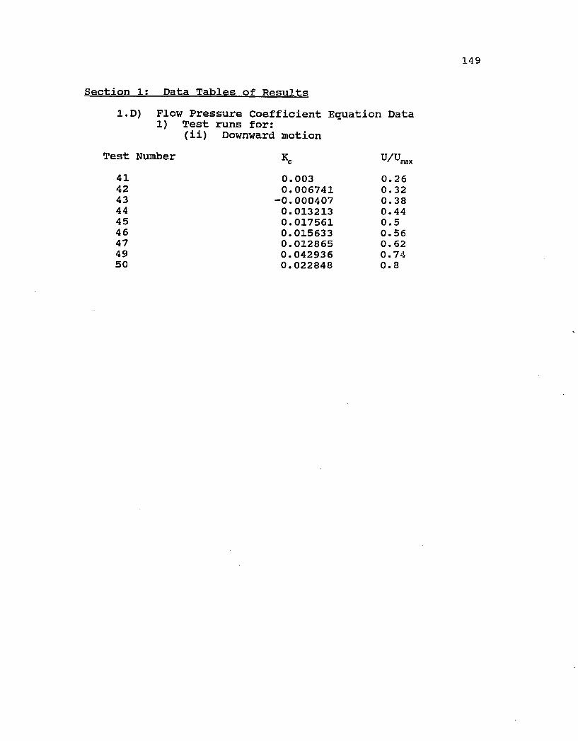
149

Section 1; Data Tables of Resultsl.D) Flow Pressure Coefficient Equation Data

1) Test runs for:(ii) Downward motion

ist Number K c % /U m a x

41 0.003 0.2642 0.006741 0.3243 -0.000407 0.3844 0.013213 0.4445 0.017561 0.546 0.015633 0.5647 0.012865 0.6249 0.042936 0.7450 0.022848 0.8

150

Section 1; Data Tables of Resultsl.E) Flow Gain Coefficient Equation Data

1) Test runs for:(i) Upward motion

Test Number AP desired(psi)51 -0.00723 1052 -0.00403 1253 -0.1208 1554 -0.2009 1755 -0.142 2056 -0.2178 2557 -0.00474 3058 -0.1968 3559 -0.00598 4060 -0.3389 45

151

Section l; Data Tables of Resultsl.E) Flow Gain Coefficient Equation Data

1) Test runs for:(ii) Downward motion

Test Number AP desired(psi)61 0.0385 -1062 0.0813 -1263 0.6819 -1564 0.1952 -1765 0.10238 -2066 -0.0329 -2567 -0.0205 -3068 0.2693 -3569 0.1636 -4070 0.24274 —45

152

Section 2 ; Graphs of Results2.A) Calibration Curves for Pressure Transducers

3 and 41) Pressure transducer 32) Pressure transducer 4

2.B) Encoder Position vs Time1) Varying speed values, upward motion2) Varying speed values, downward motion

2.C) Q/Qmax AP/P^ : Raw data set and best fit line1) Raw data for tests 31-402) Best fit lines for tests 31-40

2.D) Q/Qnax AP/Pg : Raw data set and best fit line1) Raw data for tests 41-502) Best fit lines for tests 41-50

2.E) Standard Error vs Order of the Polynomial Fit1) Tests 31-402) Tests 41-50

2.F) K, vs ü/ü„,1) Tests 31-40; third order fit2) Tests 41-50; linear approximation

2.G) Kq vs APdesired1) Positive values of desired pressure

difference2) Negative values of desired pressure

difference

153

2000 .00 -1

1 5 0 0 .0 0 -

œo_

Calibration Curve Pressure Transducer 5

2 1000.00 -

Z3œU)CD

5 0 0 .0 0 -

* R e p re s e n ts 0 to 1 5 0 0 (p s i) c lim b . R e p re s e n ts 1 4 0 0 to 0 (p s i) d e c e n t

0.00 VI f I i xr i I 1111111I I11 i 11 m I n I I u 11 M M 111 M 1111 I j I in 111 n 11 M 11 M M {I 1 M 11I I 110 ,0 0 1 .0 0 2 .0 0 3 .0 0 4 .0 0 5 .0 0 6 .0 0 7 .0 0

Voltage (V)

2.Â.1) Pressure Transducer 3

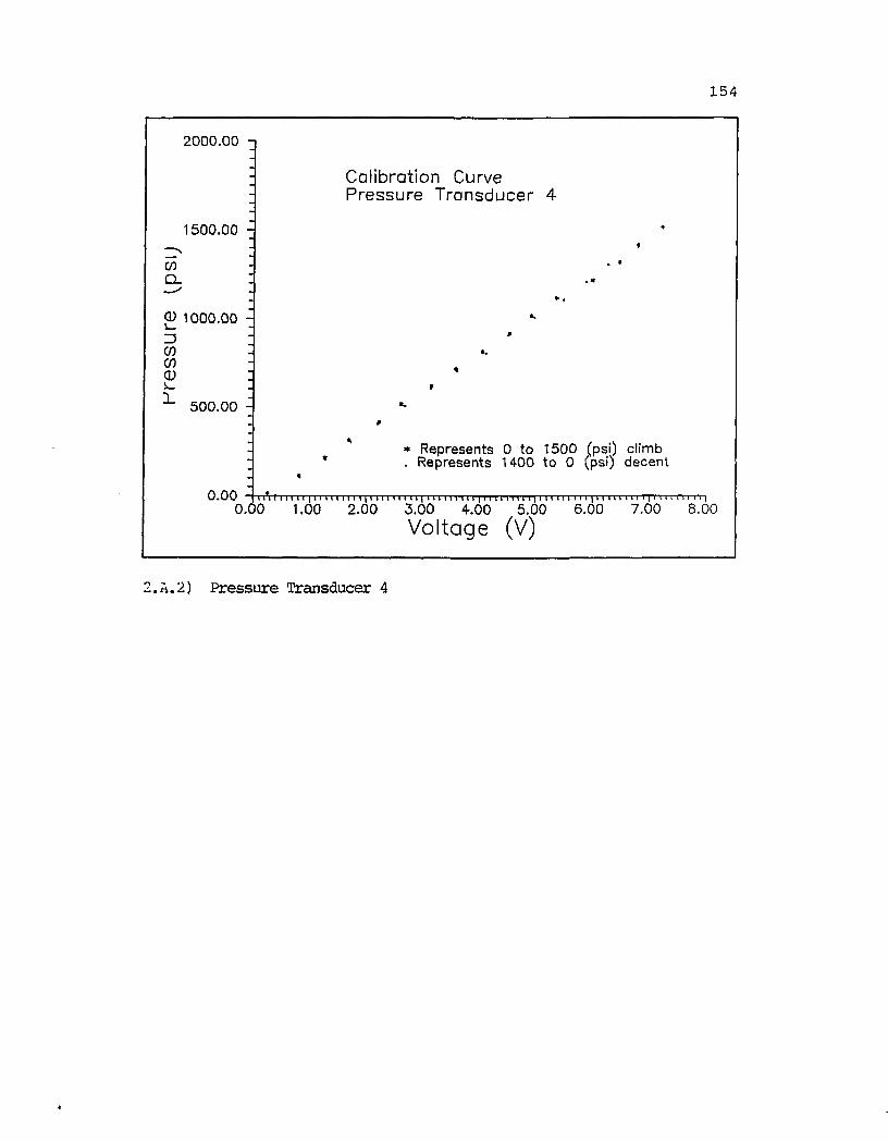
2 000 .00 -1

1 5 0 0 .0 0 -

COQ _

2 1000.00D CO CO CD

^ 5 0 0 .0 0 -

154

Calibration Curve Pressure Transducer 4

* R e p re s e n ts 0 to 1 5 0 0 (p s i) c lim b . R e p re s e n ts 1 4 0 0 to 0 (p s i) d e c e n t

0 .0 0 “ I (t ( 11111 111 i ( 1111 1111 u I i 1111 n 11111 n 111 M M 11 I p 11 111 1111 n 111 M I 111 111 111 111 0 .0 0 1 .0 0 2 .0 0 3 .0 0 4 .0 0 5 .0 0 6 .0 0 7 .0 0 8 .0 0

Voltage (V)

2.A.2) Pressure Transducer 4

155

Il lui euüniy o p ccu

2000.00 1

1 5 0 0 .0 0

cotnO0_ 1000.00k_0)■oooc_ü Test Runs 31

Upward Motion Actuator 2 Varying Speed

4 05 0 0 .0 0 -

0.00 24.00.0 8.0 1 6 .0Time ( se c o n d s )

2.3.1) Varying Speed Values, Upward Motion

156

CoenO3_<D•OOoc_u

2000.00 -,

Test Runs 41 — Downward Motion Actuator 2 Varying Speed

5 0

1500.00 -

1000.00

500.00 -

Increasing Speed

0.000.0 2.0 4.0 6.0Time ( s e c o n d s )

8.0

.3.2) Varying Speed Values, Downward Motion

157

0.0400

0.0300

0.0200

O 0.0100

lOfMM0.0000

- 0.0100

- 0.0200 -0.5600 -0.4000 -0.3200-0.6400 -0.4800( P 3 - P 4 ) / P s

2.C.1) lîav; Data For Tests 31-40

158

0.0400

0.0300

0.0200

a 0.0100

0.0000

-0.0100

- 0.0200 TU 11 II' 111 m 11 n 'n I m I n 11111111 r I m 11 III I H I H H 1111 m 111111111 m I III 11 n i0.5600 -0.4800 -0.4000 -0.3200( P 3 - P 4 ) / P s

-0.4000-0.6400

2.C.2) Best Fit Lines For Tests 31-40

159

0.0200

- 0.0000

- 0.0200 :

X DE

a -0 .0 4 0 0 :

o-0 .0 6 0 0 :

-0 .0 8 0 0 :

-0 .1000 11111111 n IT 11111 iTi 11111 m u 11 H1 l'u 1111111 m TTi n 11 m 1111 m i n i m n n n n |-0 .8 8 0 0 -0 .8 0 0 0 -0 .7 2 0 0 -0 .6 4 0 0 -0 .5 5 0 0

( P 3 - P 4 ) / P s

2.D.1) Raw Data For Tests 41-50

150

0.0200 q

- 0.0000

- 0.0200

O -0.0400

-0.0600

-0.0800

— 0 . 1 0 0 0 ~ 1 1 1 11 —0.8800 -0.8000 -0.7200( P 3 - P 4 ) / P s

-0.6400 -0.5500

7..D.2) Best Fit Lines For Tests 41-50

161

0.0070 q Standard Error vs Order o f Polynom ial Fit

0.0060 z

0.0050 -EOi_

w 0.0040 z■DT? 0.0030 -3 o4-'(/)0.0020 4

0.0010 -E

Objective: Determine the order of the best• It t ■

40polynomial fit between Kc and U/Umox. Tests 31

0.0000 TT T T T T T T T T T T T T T T T T rrrrrrT T T T T T T T rrrrT T T T T T T T T T T T T T T T rrrT T T T T T T T T T T T T T rrrrT T X T T ri) 1 2 3 4

Order of P o lynom ia l

2.E.1) Tests 31-40

0.0030 q stan d ard Error vs Ord^r o f Polynom ial Fit

0.0028 -

162

ÜJ0.0026 -

Oc 0.0024D

0.0022 -

)Objective: Determine the order of the best

polynomial fit between Kc ond U/Umox. Tests 41 — 50

0 . 0 0 2 0 j 111 r 1111111111111111111 n i it vi i n i i i i i i i i i i i i i i i i i n i i im r r i 111111111111 11 r n i jt| 0 1 2 3 4

Order of P o lynom ia l

!) Tests 41-50

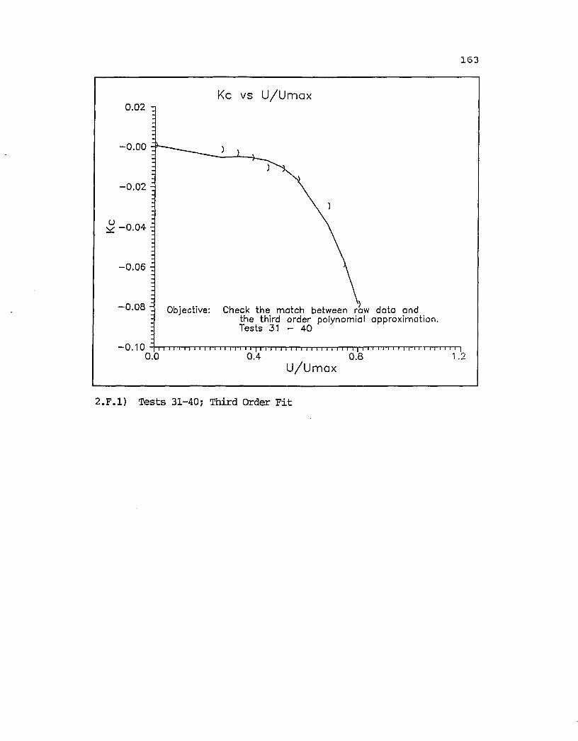
163

Kc VS U / U m a x0.02 3

- 0.00 -

- 0.02

^ -0 .0 4

-0 .0 6

-0 .0 8 O b jec tiv e : C h e c k t h e m a tc h b e tw e e n raw d a t a a n dth e th ird o r d e r p o ly n o m ia l a p p r o x im a tio n . T e s ts 31 - 4 0T e s ts 31

-0.10 4-1 0.0 0.4 0.8U / U m a x

2.F.1) Tests 31-40; Third Order Fit

164

Kc VS U / U m a x0 .0 5 q

0.04

0 .0 3

0.02

0.01

0.00O b je c tiv e : C h e c k t h e m a tc h b e tw e e n raw d a t a a n d

th e l in e a r a p p r o x im a tio n .T e s t s 41 - 5 0- 0.01

- 0.02 - 0.0TniTi i I u ' l n III (II11H n 1111 III n I n n 111II11 n III n n n iv) I n n i u n n M IS rv 11 n 111 n n Tn n i 1 1 1 1 1

0 .2 0 .4 0.80.6U / U m a x

2.p.2) Tests 41-50; Linear Approximation

165

0.00 n

- 0.10

D - 0 .3 0 -

^ - 0 .4 0 -

- 0 .5 00.00 50.0010.00 20 .00 30 .00 40.00Desired Pressure Difference (psi)

2.G.1) Positive Values Of Desired Pressure Difference

166

O 0.20

- 0.00

- 0.20

- 6 0 .0 0 - 5 0 .0 0 - 4 0 .0 0 - 3 0 .0 0 - 2 0 .0 0 - 1 0 .0 0 0.00Desired P ressure Difference (psi)

2.G.2) Negative Values of Desired Pressure Difference

167

APPENDIX C — Equipment Specifications

168

Equipment Specifications1) Dead Weight Tester2) Pressure transducers; series PX-3 023) AD524BD Specifications4) Analog input instrumentation panel: PCI-20019M-1A5) Position Encoder: M25D

169Deadweight Tester

Omega Type DWT 13 05 DInformation from; "Installation and Maintenance Manual for the Omega Type DWT 1305D Dead Weight Tester"

Specifications ; Accuracy;

Deadweight;Pump;

Operating Fluids:

Combined tolerance of weights and pistons and cylinder assemblies within 0.1% of readingNon-magnetic die cast zinc alloyTwo stage, lever operated generates10,000 psi (70,000 kPa)Light grade oils, automotive petroleum base

170Series PX3 02 — Pressure Transducer

Omega Engineering, Inc.Omega Technologies Company One Omega Drive, Box 4047 Stamford, Connecticut 06907-0047

Specifications;Excitation: Output:Proof Pressure:Input Impedance: Output Imedance:

Performance:Accuracy:

Zero Balance:Construction:

Body/Diaphragm: Pressure Port: Cavity Volume: Weight:

Nominal 10 volts DC 100 mv full scale (lOmv/v ± 1%) 2 X full scale or 15,000 psi (whichever is less)1200 ohms minimum 500 ohms nominal

+ 0.5% full scale at 75 F (linearity, hysteresis, and repeatab ility)+ 2% of full scale at + 75 F

17-4 ph stainless steel Male 1/4-18 NPT 0.030 cubic inches Approximate, 2 ounces

171AD524BD Specifications

Analog DevicesPrecision Instumentation Amplifier

Specifications: Noise;Nonlinearity:Offset:Drift:Gains:

0.3 microvolts p-p 0.1 Hz to 10 Hz 0.0003% (G=l)Low offset voltage 50 microvolts Low offset voltage .5 microvolts/C Pin programmable gains 1, 10, 100, 1000

For fixed gains of 1, 10, 100, or 1000 the AD524Bd does not require any outside components. With the addition of external resistors any gain between 1 and 1000 may be programmed.The AD524BD has two terminals available for connection as a null offset.

172PCI-20019M-1A Analog Input Instrumentation Module

Burr-Brown Analog Input Module

Specifications :Bits:Channels:Dimensions ;

Voltage range:

12-bit analog-to-digital converter Input multiplexer with a flexible channel scanner 3.9(in) X 3.9(in) cardVoltage range is set with the following jumper connections:JumperW1W2W3W4W5

+10 voltsoutinoutinout

173Position Encoder

BEI Motion Systems Company M25-X-LSS16384N-GD1-X-E-C25-X-5 Information from; "Optical Encoders"

Specifications :Type;Light Source:

Operating Temperature: Options:

Optical encoderSingle infrared range Light Emitting Diode, LED, demagnification-0 C to +70 CFront face mounting Rear face cable extension