System Aspects of Probabilistic DBs Part II: Advanced Topics Magdalena Balazinska, Christopher Re...

System Aspects of Probabilistic DBs Part II: Advanced Topics

Magdalena Balazinska,Christopher Re and Dan Suciu

University of Washington

Recap of motivation

• Data are uncertain in many applications– Business: Dedup, Info. Extraction– Data from physical-world: RFID

2

Probabilistic DBs (pDBs) manage uncertainty

Integrate, Query, and Build Applications

Value: Higher recall, without loss of precision

DB Niche: Community that knows scale

3

Highlights of Part II

• Yesterday: Independence• Today: Correlations and continuous values.

– Lineage and view processing

– Events on Markovian Streams

– Sophisticated factor evaluation

– Continuous pDBs

GBs with materialized views

GBs of correlated data

Highly correlated data

Correlated, Continuous values

Technical Highlights

4

Overview of Part II

• 4 Challenges for advanced pDBs

• 4 Representation and QP techniques1. Lineage and Views2. Events on Markovian Streams3. Sophisticated Factor Evaluation4. Continuous pDbs

• Discussion and Open Problems

5

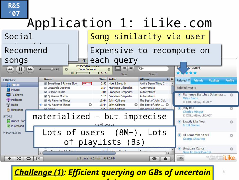
Application 1: iLike.com

materialized – but imprecise – view

Lots of users (8M+), Lots of playlists (Bs)

R&S ‘07

Challenge (1): Efficient querying on GBs of uncertain data

Social networking site Song similarity via user preferences

Expensive to recompute on each queryRecommend songs

6

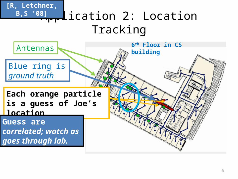
Application 2: Location Tracking

Each orange particle is a guess of Joe’s location

Blue ring is ground truth

Antennas

Guess are correlated; watch as goes through lab.

6th Floor in CS building

[R, Letchner, B,S ’08]

7

Application 2: Location Tracking

Each orange particle is a guess of Joe’s location

Blue ring is ground truth

Antennas 6th Floor in CS building


Challenge (2): track correlations across timeJoe’s location at time t=9

depends on his location at t=8

Guess are correlated; watch as goes through lab.

8

Application 3: the Census[Anotva,Koch&Olteanu ’07]

Each parse has own probability

SSN is a key

Product of all uncertainty

Challenge (3): Represent highly correlated relational data

185 or 785?

185 or 186?

Choices are correlated

9

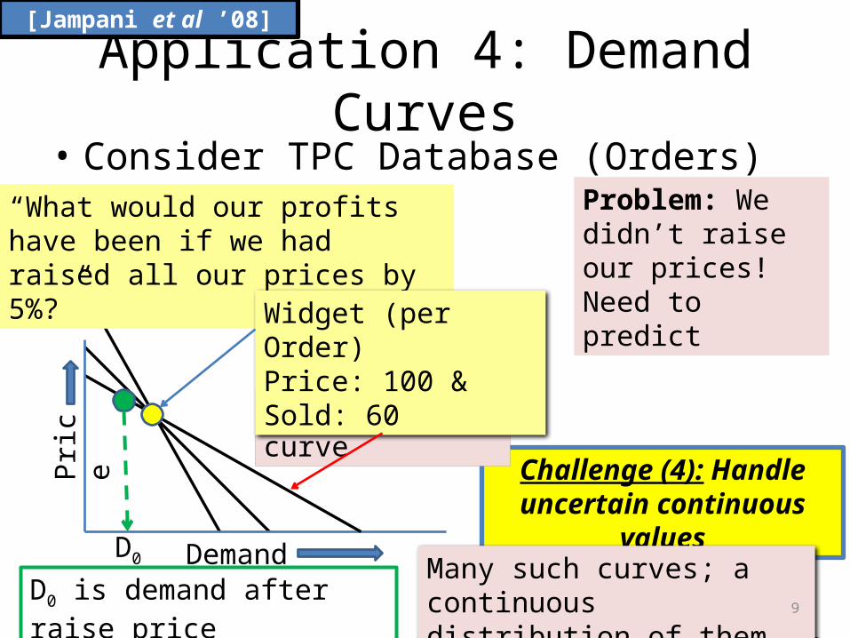
Application 4: Demand Curves• Consider TPC Database (Orders)

Challenge (4): Handle uncertain continuous values

“What would our profits have been if we had raised all our prices by 5%?”

Problem: We didn’t raise our prices! Need to predict

linear demand curve

[Jampani et al ’08]

Demand

Pric

e

Widget (per Order)Price: 100 & Sold: 60

D0 is demand after raise priceMany such curves; a continuous distribution of them.

D0

10

pDBs Challenges Summary

This is the main tension!

Materialize all worlds is faithful, but not efficientSingle possible world efficient, but not faithful

• Challenges• Efficient Querying• Track complex correlations• Continuous Values

Faithful: Model important correlations

Efficiency: Storage and QP

11

Overview of Part II

• 4 Challenges for advanced pDBs

• 4 Representation and QP techniques1. Lineage and Views2. Events on Markovian Streams3. Sophisticated Factor Evaluation4. Continuous pDbs


12

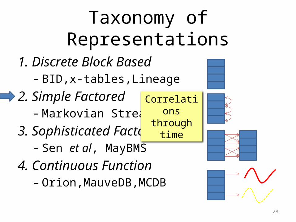
Taxonomy of Representations

1. Discrete Block Based– BID,x-tables,Lineage

2. Simple Factored– Markovian Streams

3. Sophisticated Factored– Sen et al, MayBMS

4. Continuous Function– Orion,MauveDB,MCDB

Outline for the technical portion

Correlations via views

Correlations through time

Complex Correlations

Continuous Values and correlations

13






Correlations via views

14

Discrete Block-based Overview

• Brief review of representation & QP

• Views in Block-based databases

• 3 Strategies for View Processing1. Eager Materialization (Compile time)2. Lazy Materialization (Runtime)3. Approximate Materialization (Compile time)

Allow GBs sized pDBs

Views introduce correlations

15

Block-based pDB

Object Time Person P

Laptop77 9:07John 0.62

Jim 0.34

Book302 9:18

Mary 0.45

John 0.33

Fred 0.11

HasObjectp

Keys ProbabilityNon-keys

[Barbara et al’92][Das Sarma et al 06], [Green&Tannen06],[R,Dalvi,S06]

Semantics distribution over possible worlds

Object Time Person

Laptop77 9:07 John

Book302 9:18 Mary

0.62 * 0.45 = 0.279

16

Intensional Query EvaluationGoal: Make relational ops compute expression f

QP builds Boolean Formulae fQP builds Boolean Formulae f

[Fuhr&Roellke’97, Graedel et al. ’98, Dalvi & S ’04, Das Sarma et al 06][Fuhr&Roellke’97, Graedel et al. ’98, Dalvi & S ’04, Das Sarma et al 06]

Pr[q] = Pr[f is SAT].

Each tuple variable

s

v f

v f

JOIN

v1 f1

v1 v2 f1˄f2

v2 f2

P

v f1

v f2

v f1 ˅ f2 ˅ …

Internal Lineage

Projection eliminates duplicates

q1p2

Views in Block-based pDBs by exampleChef Restaurant P

Tom D. Lounge 0.9

Tom P .Kitchen 0.7

Restaurant DishD. Lounge Crab

P. Kitchen Crab

P. Kitchen Lamb

W(Chef,Restaurant) WorksAt

S(Restaurant,Dish) Serves

R(Chef,Dish,Rate) Rated

V(c,r) :- W(c,r),S(r,d),R(c,d,’High’)

“Chef and restaurant pairs where chef serves a highly rated dish”

Chef Restaurant P

Tom D. Lounge 0.72 p1˄q1

Tom P. Kitchen 0.602 p2˄ (q1˅q2)

p1q2

17

Chef Dish Rate PTom Crab High 0.8Tom Lamb High 0.3

[R&S 07]

{c →`Tom’, r → `D. Lounge’, d →`Crab’}

0.72 = 0.9 * 0.8

q1p2

Views in BID pDBsChef Restaurant P

Tom D. Lounge 0.9

Tom P .Kitchen 0.7


P. Kitchen Crab

P. Kitchen Lamb




Chef Restaurant P

Tom D. Lounge 0.72 p1˄q1


p1q2

18

View has correlations

Chef Dish Rate P

Tom Crab High 0.8

Tom Lamb High 0.3

[R&S 07]

Thm [ R,Dalvi,S ’07] BID are complete with the addition of views



19



• Views in Block-based databases– Views introduce correlations.

• 3 Strategies for View Processing1. Eager Materialization (Compile time)2. Lazy Materialization3. Approximate Materialization

Allow scaling to GBs of relational data

20

Eager Materialization of BID Views

• Why?1. Lineage can be much larger than view2. Can do expensive prob. computations off-line3. Use view directly in safe-plan optimizer4. Interleave Monte-Carlo Sampling with safe-plan

Example coming…[R&S 07]

Catch: need that tuples are independent for any instance.independence test

Chef Restaurant P

Tom D. Lounge 0.72

Tom P. Kitchen 0.602

Chef Restaurant P

Tom D. Lounge 0.72 P1˄q1


pDB analog of Materialized Views

Allows GB scale pDB processing

Idea: Throw away the lineage, process views

Chef Restaurant PTom D. Lounge 0.72 p1˄q1


q1p2

Eager Materialization of pDB ViewsChef Restaurant P

Tom D. Lounge 0.9

Tom P .Kitchen 0.7


P. Kitchen Crab

P. Kitchen Lamb






p1q2

21

Can we understand w.o. lineage?

Chef Dish Rate P

Tom Crab High 0.8

Tom Lamb High 0.3

[R&S 07]

Not every probabilistic view is good for materialization!

q1p2

Eager Materialization of pDB ViewsChef Restaurant P

Tom D. Lounge 0.9

Tom P .Kitchen 0.7


P. Kitchen Crab

P. Kitchen Lamb




“chefs that serve a highly rated dish”

p1q2

22

Can we understand w.o. lineage?

Chef Dish Rate P

Tom Crab High 0.8

Tom Lamb High 0.3

[R&S 07]

V2(c) :- W(c,r),S(r,d),R(c,d,’High’)

Where could such a tuple live?

V2 is a good choice for materialization

Obs: if no prob. tuple shared by two chefs, then they are independent

23

• Thm: Deciding if a view is representable as a BID is decidable & NP-Hard (Complete for P2)

• Good News: Simple but cautious test

• Thm: If view has no self-joins, test is complete.

Is a view good or bad?

V1(c,r) :- W(c,r),S(r,d),R(c,d,’High’)V2(c) :- W(c,r),S(r,d),R(c,d,’High’)

In wild, practical test almost always works

[R&S 07] Allows GB+ Scale QP

Test: “Can a prob tuple unify with different heads?”

NB: Also, can take into account query q, i.e. can we use V1 without the lineage to answer q?

Good!

24



• Views in Block-based databases– Views introduce correlations.

• 3 Strategies for View Processing1. Eager Materialization2. Lazy Materialization (Runtime test)3. Approximate Materialization

25

Lazy Materialization of Block Views

• In Trio, queries views• Compute probs lazily• Separate confidence

computation from QP• Memoization

[Das Sarma et al 08]

Reuse/memoization + Independence Check

Check on lineage (instance data) Compute only onceCond: z and y independent of x1, x2

(z ˄ (x1 ˅ x2)) ˅ (y ˄ (x1 ˅ x2))

NB: Technique extends to complex queries

26

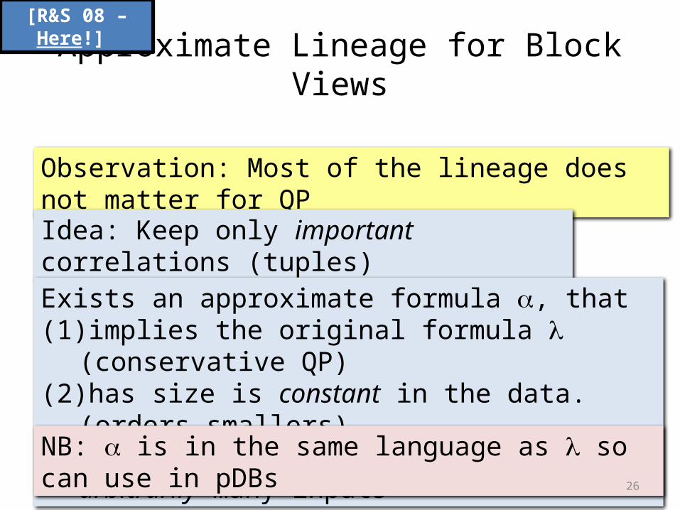
Approximate Lineage for Block Views[R&S 08 – Here!]

Observation: Most of the lineage does not matter for QP

Idea: Keep only important correlations (tuples)

Exists an approximate formula a, that (1) implies the original formula l (conservative QP)(2) has size is constant in the data. (orders smallers)(3) agrees with original func. l on arbitrarily many inputs

NB: a is in the same language as l so can use in pDBs

27

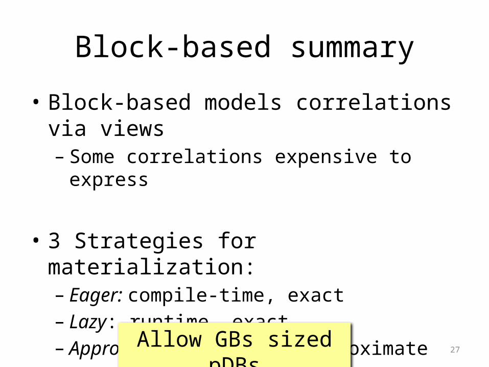
Block-based summary

• Block-based models correlations via views– Some correlations expensive to express

• 3 Strategies for materialization:– Eager: compile-time, exact– Lazy: runtime, exact– Approximate: runtime, approximate

Allow GBs sized pDBs

28






Correlations through time

Example 1: Querying RFID29

C B

A

DE

Joe entered office 422 at t=8

Query: “Alert when Joe enters 422”

i.e. Joe outside 422, inside 422

[R,Letchner,B&S’07] [http://rfid.cs.washington.edu][R,Letchner,B&S’07] [http://rfid.cs.washington.edu]

Correlations: Joe’s location @ t=9 correlated with location @ t=8

Uncertainty: Missed readings. Markovian correlations

If we know t=8 then learning t=7 gives no (little) new info about t=9

Joe has a tag on him

Sensors in hallways

30

Tag t Loc P

Joe 7 422 0.6

Hall4 0.4

Joe 8 422 0.9

Hall5 0.1

Sue 7 … …

Capturing Markovian Correlations[R, Letchner, B,S ’08]

422 Hall4422 1.0 0.75Hall5 0.0 0.25

Time = 7

Tim

e =

8 Loc0.60.4

Loc0.90.1=

Conditional Probability table (CPT)

NEW: matrix per consecutive timesteps

Markov Assumption

add to 1 Time = 8

31

other 422 Hall4

{} 0.1 0.6

{1}

{2} 0.3

{1,2}

Computing when Joe Enters a Room

Joe Final

Joe in Hall4 Joe in 4221 2Accept t=8 with p = 0.3

Alert me when Joe enters 422


Tag t Loc P

Joe 7 422 0.6

Hall4 0.4

Joe 8 422 0.9

Hall5 0.1

Sue 7 … …

422 Hall4422 1.0 0.75Hall5 0.0 0.25

Time = 7

Tim

e =

8

other 422 Hall4

{} 0.6

{1} 0.4

{2}

{1,2}

Last Time

Last seen

stat

esCorrelations map to simple matrix algebra with tricks

other 422 Hall4

{} 1.0

{1}

{2}

{1,2}

0.4 * 0.75 = 0.3

32

Markovian Streams (Lahar)

• “regular expression” queries efficiently

• Streaming: “Did anyone enter room 422?”– independence test, on an event language

• “Safe queries” involve complex temporal joins– Time size(archive), i.e. not streaming, but PTIME– Event queries based on Cayuga– #P-Hard boundary found as well


Streaming in real-time

33






Complex Correlations

34

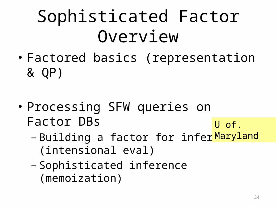
Sophisticated Factor Overview

• Factored basics (representation & QP)

• Processing SFW queries on Factor DBs– Building a factor for inference (intensional eval)– Sophisticated inference (memoization)

• The MayBMS System

U of. Maryland

35

Sophisticated FactoredAD ID Model Price

201 Civic (EX) 6000 1.0

203 Civic 1000 0.6

Corolla 0.4

[Sen,Desphande, Getoor 07] [SDG08]

Model Pollutes

Civic (EX) High 1.0

Civic (Hybrid)

Low 1.0

Civic Low 0.7

High 0.3

Corolla High 1.0

Pollutes Tax

Low 1000

High 2000

“If I buy car 203, how much tax will I pay?”

Challenge: Dependency (correlations) in the data between extracted car model and tax amount.

Extracted Ambiguous

36

TMPM

Factor graphs Semantics

Model (M) (MP) Tax

(T)

Model PriceCivic 1000 0.6

Corolla 0.4

Model Pollutes

Civic Low 0.7

High 0.3

Corolla High 1.0

Pollutes Tax

Low 1000

High 2000

Factors

Generalization of Bayes Nets Relevant data from previous slide

Joint(m,p,t) =M(m)MP(m,p)T(p,t)“If I buy this car how much tax will I pay?”

Equivalent: Graphical model Joint Probability Factors

Answer: ∑m,pM(m)MP(m,p)T(p,t)

37

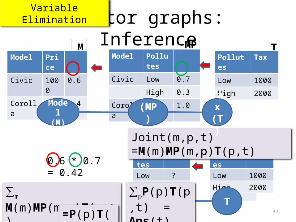
M MP T

Tax P

1000 0.42

2000 0.58

Pollutes

Low 0.42

High 0.58

Factor graphs: InferenceModel PriceCivic 1000 0.6

Corolla 0.4

Model Pollutes

Civic Low 0.7

High 0.3

Corolla High 1.0

Pollutes Tax

Low 1000

High 2000

Variable Elimination

Pollutes

Low 0.42

High ?

Pollutes Tax

Low 1000

High 2000

0.6 * 0.7 = 0.42Pollutes

Low ?

High ?

P T

Joint(m,p,t) =M(m)MP(m,p)T(p,t)

Model (M) (MP) Tax

(T)

∑m M(m)MP(m,p)T(p,t)

=P(p)T(p,t)

∑pP(p)T(p,t) = Ans(t)

38

Factors can encode functions

More general aggregations & correlations

f1˄f2

f1 f2 Out

0 0 0

0 1 0

1 0 0

1 1 1

Factors can encode logical fns

f1 ˅ f2

f1 f2 Out

0 0 0

0 1 1

1 0 1

1 1 1

Think of factors as functions.

f2f1

˄

f2f1

˅

39

Sophisticated Factor Overview

• Factored basics (representation & QP)

• Processing SFW queries on Factor DBs– Building a factor for inference (intensional eval)– Sophisticated inference (memoization)

• The MayBMS System

U of. Maryland

40

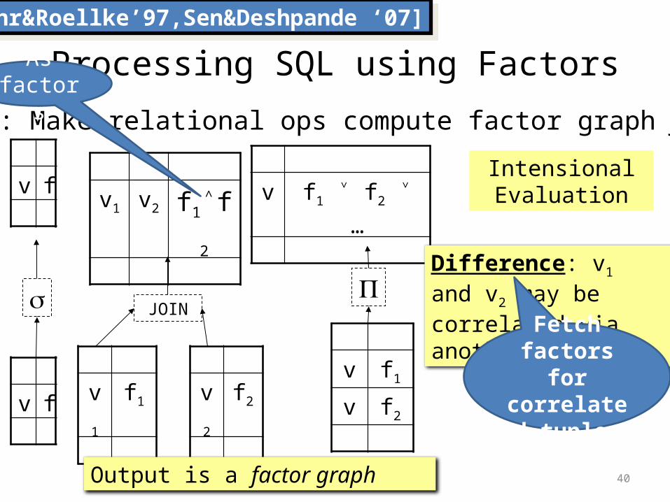
Processing SQL using FactorsGoal: Make relational ops compute factor graph f

[Fuhr&Roellke’97,Sen&Deshpande ‘07][Fuhr&Roellke’97,Sen&Deshpande ‘07]

s

v f

v f

JOIN

v1 f1

v1 v2 f1˄f2

v2 f2

P

v f1

v f2

v f1 ˅ f2 ˅ …

Difference: v1 and v2 may be correlated via another tuple

Fetch factors for correlated

tuples

Output is a factor graph

Intensional Evaluation

As factors

41

Smarter QP: Factors are often shared

All civic (EX) share common pollutes attribute.

AD ID Model Price

201 Civic (EX) 6000 1.0

203 Civic 1000 0.6

Corolla 0.4

Model Pollutes

Civic (EX) High 1.0

Civic (Hybrid)

Low 1.0

Civic Low 0.7

High 0.3

Corolla High 1.0

Pollutes Tax

Low 1000

High 2000

Naïve Variable Elimination may perform this computation several times…

[Sen,Desphande & Getoor ’08 -- HERE]

42

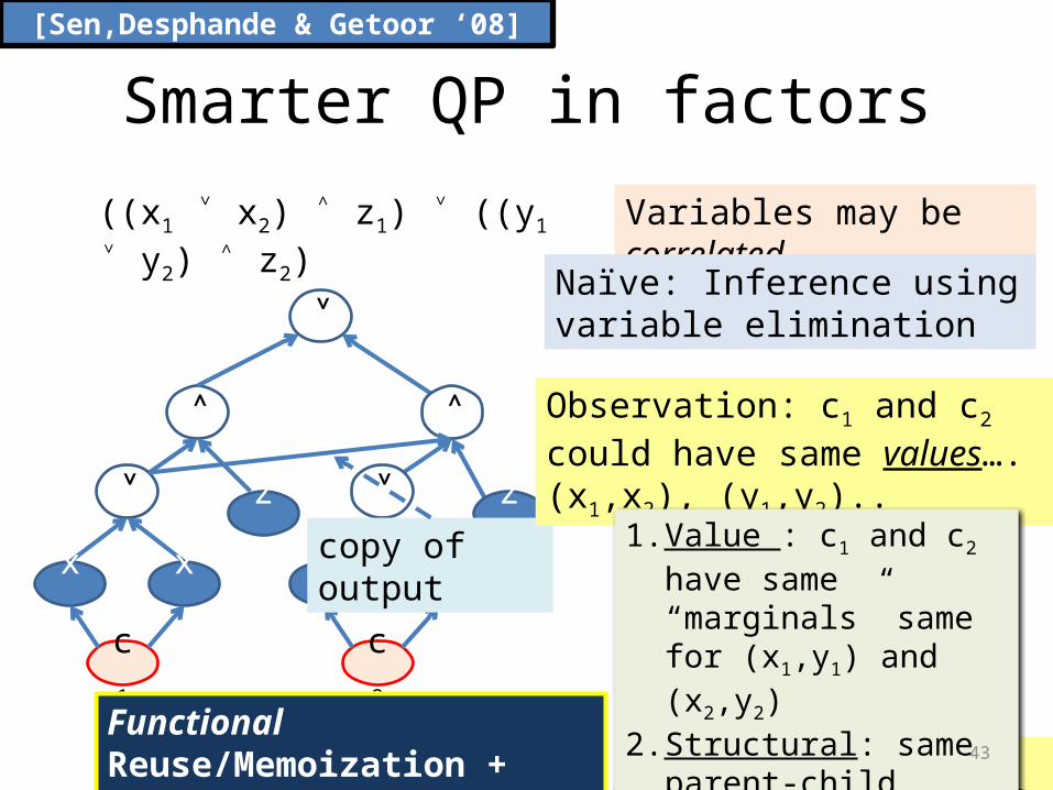
Smarter QP in factors

Variables may be correlated

Naïve: Inference using variable elimination

[Sen,Desphande & Getoor ‘08]

((x1 ˅ x2) ˄ z1) ˅ ((y1 ˅ y2) ˄ z2)

˅

y1 y2x2x1

˅

˄

z1 z2

˅

˄

c2c1

Observation: c1 and c2 could have same values….

1. Value : c1 and c2 have same “marginals” same for (x1,y1) and (x2,y2)

2. Structural: same parent-child relationship

Likely due to sharing

43

Smarter QP in factors

Variables may be correlated

[Sen,Desphande & Getoor ‘08]

((x1 ˅ x2) ˄ z1) ˅ ((y1 ˅ y2) ˄ z2)

˄

z1 z2

˅

˄

˅

x1 x2

c1

˅

y1 y2

c2

Functional Reuse/Memoization + Independence

copy of output

Observation: c1 and c2 could have same values….(x1,x2), (y1,y2)..

Likely due to sharing

1. Value : c1 and c2 have same “marginals” same for (x1,y1) and (x2,y2)

2. Structural: same parent-child relationship

Naïve: Inference using variable elimination

44

Interesting Factor facts

• Factor graph is a tree, then QP is efficient• Exponential in the worst case• NP-Hard to pick best tree

• If query is safe, then factor graph is a tree• The converse does not hold!• Obs: Good instance or constraint not

known to optimizer, e.g. FD.

[Sen,Desphande ‘07] [SD&Getoor08]

45

Factors: the Census[Anotva,Koch&Olteanu ’07]

Different probs for each cardUnique SSN Correlations

Represent succinctly

Possible word: any subset of product of all these tables.

Name SSNSmith 785:0.8 or 185:0.2Brown 185:0.4 or 186:0.6

T1.Name

Smith

T1.Married

Single 0.7

Married 0.3

T2.Name

Brown

T2.Married Pr

Single 0.25

Married 0.25

Divorced 0.25

Widowed 0.25

T1.SSN T2.SSN

185 186 0.2

785 185 0.4

785 186 0.4

T1

T2

46

MayBMS System

• MayBMS represent data as factored– SFW QP is similar– Variable Elimination (Davis-Putnam)

[Anotva,Koch&Olteanu ’07][Koch’08][Koch & Olteanu ’08]

Big difference: Query Language.

1. Compositional. Language features together arbitrarily.2. Confidence Computation explicit in QL.3. Predication on Probabilities

“Return people whose probability of being a criminal is in [0.2,0.4]”

47


1. Discrete Block Based– BID, x-tables, Lineage


3. Sophisticated Factored– Sen et al., MayBMS, BayesStores

4. Continuous Function– Orion, MauveDB, MCDB

Continuous Values and correlations

48

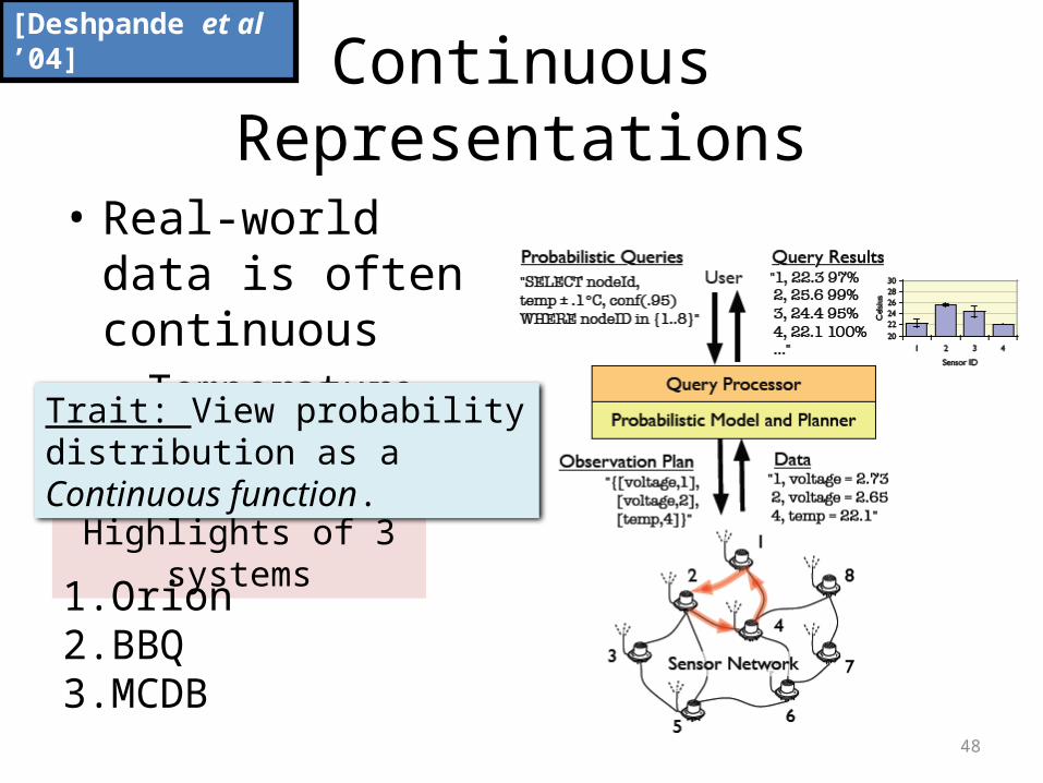
Continuous Representations

• Real-world data is often continuous– Temperature

[Deshpande et al ’04]

Highlights of 3 systems

Trait: View probability distribution as a Continuous function.

1. Orion2. BBQ3. MCDB

49

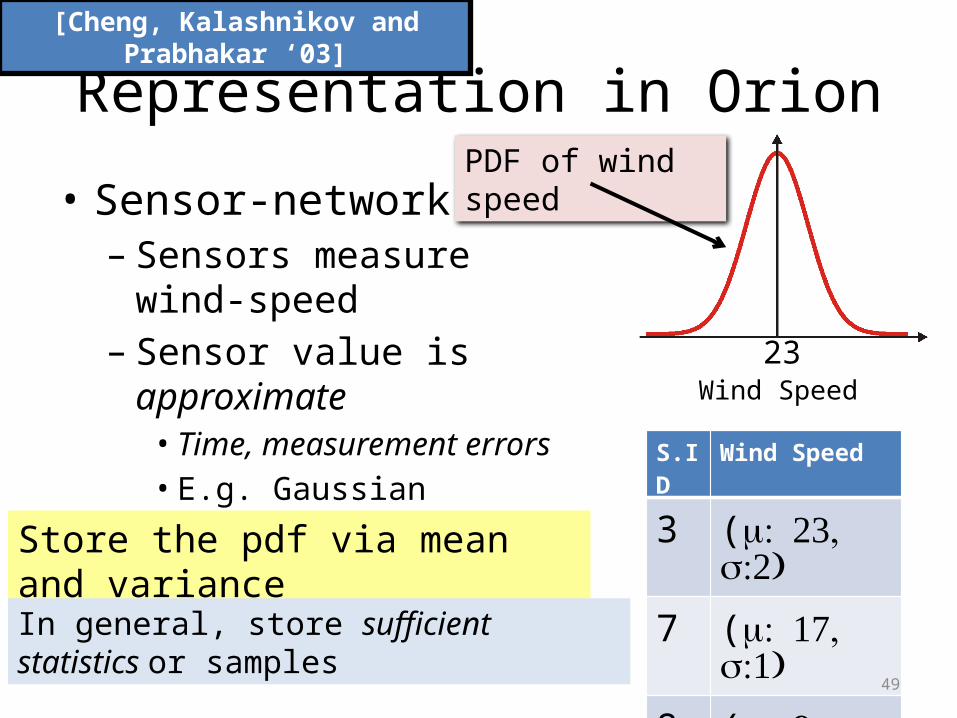
Representation in Orion

• Sensor-networks– Sensors measure wind-speed– Sensor value is approximate

• Time, measurement errors• E.g. Gaussian

[Cheng, Kalashnikov and Prabhakar ‘03]

Store the pdf via mean and variance

In general, store sufficient statistics or samples

S.ID Wind Speed

3 ( : 23, m:2)s

7 ( : 17, m:1)s

8 ( : 9, m:5)s

Wind Speed23

PDF of wind speed

50

Queries on Continuous pDBs

• Value-based non-aggregate– “What is the wind speed recorded by sensor 8?”

• Entity-based non-aggregate– “Which sensors have wind speed in [10,20] mph?”

• Value-based aggregate– “What is the average wind speed on all sensors?”

• Entity-based aggregate– “Which sensor has the highest wind speed?”


PDF of sensor 8

(3, 0.06),(7,0.99),…

PDF of average

(3, 0.95),(7, 0.04),..

51

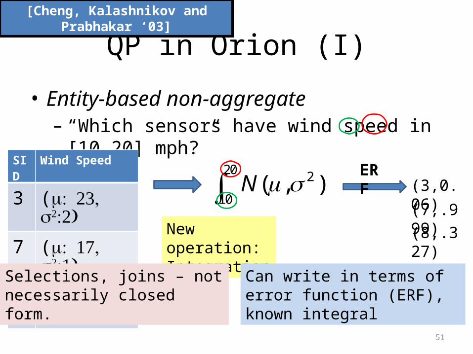
QP in Orion (I)

• Entity-based non-aggregate– “Which sensors have wind speed in [10,20] mph?”


SID Wind Speed

3 ( : 23, ms2:2)

7 ( : 17, ms2:1)

8 ( : 9, ms2:5)

20 2

10( , )N

ERF(3,0.06)

(7,.999)(8,.327)New operation:

Integration

Can write in terms of error function (ERF), known integral

Selections, joins – not necessarily closed form.

52

BarBie-Q (BBQ), a tiny model

• Wind-speeds not independent

• model-based-view– Hide the uncertainty,

correlations

[Deshpande et al ’04]

Physically close, so speeds close too

User queries the model

DB may (1) acquire new data, or (2) use model to predict values or some combination

53

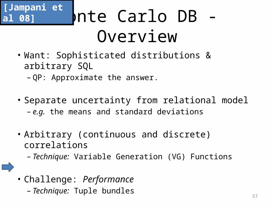
Monte Carlo DB - Overview

• Want: Sophisticated distributions & arbitrary SQL – QP: Approximate the answer.

• Separate uncertainty from relational model– e.g. the means and standard deviations

• Arbitrary (continuous and discrete) correlations– Technique: Variable Generation (VG) Functions

• Challenge: Performance– Technique: Tuple bundles

[Jampani et al 08]

54

Declaring Tables in MCDB

• Consider a patient DB with blood pressures

[Jampani et al 08]

CREATE TABLE SBP_DATA FOR EACH p in PATIENTS WITH SBP as NORMAL (SELECT s.mean, s.std FROM SBP_PARAM s) SELECT p.PID, p.GENDER, b.VALUE FROM SBP b

Declares a random sample

Normal, params from SBP_PARAM.More generally, can depend on patient

NORMAL can be replaced with an arbitrary function, called a VG function

55

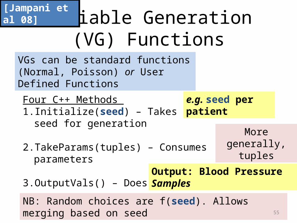
Variable Generation (VG) Functions[Jampani et al 08]

Four C++ Methods 1. Initialize(seed) – Takes as input a seed for generation

2. TakeParams(tuples) – Consumes parameters

3. OutputVals() – Does the MC iteration

4. Finalize()

NB: Random choices are f(seed). Allows merging based on seed

Output: Blood Pressure Samples

VGs can be standard functions (Normal, Poisson) or User Defined Functions

e.g. seed per patient

More generally, tuples

56

A sophisticated VG Function

“What would our profits have been if we had raised all our prices by 5%?”

linear demand curve

Demand

Pric

e

Widget (per Order)Price: 100 & Sold: 60

D0 is demand w. Raised Price

Procedure:1. Randomly generate line

through Widget Point

2. Return d0

According to prior

Price 105

d0

On TPC Data

[Jampani et al 08]

57

Monte Carlo DB - Overview

• Want: Sophisticated distributions & arbitrary SQL – QP: Approximate the answer.

• Separate uncertainty from relational model– e.g. the means and standard deviations

• Arbitrary (continuous and discrete) correlations– Technique: Variable Generation (VG) Functions

• Challenge: Performance– Technique: Tuple bundles

[Jampani et al 08]

58

MCDB QP: tuple bundles

• Smarter: Tuple bundles

[Jampani et al 08]

Patient Gender BP

123 M 160

130

170

456 F 110

Patient Gender

123 M

456 F

VG100s-1000s of samples

Patient Gender BP[]

123 M 160,130,170

456 F 110

Patient & Gender constant – bundle BPs together

“Blood pressure higher than 135?”

59

MCDB: Late Materialization

Patient Gender BP

123 M 160

130

170

456 F 110

Patient Gender123 M

456 F

VG

“Average BP of all patients who had a consult with a doctor on the third floor”

Rest of SQL processing

Slow! Many copies of same tuple!

Keep the random seeds instead of many tuples.

Remove duplicates, based on seed

[Jampani et al 08]

Result: sampling on much smaller set.

60

Representation & QP Summary

• Discrete Block Based– View Processing

• Simple Factored– Temporal (simple) correlations

• Sophisticated Factored– General Correlations

• Continuous Function– Complex correlations– Measurement errors

61

Representation & QP Summary

• 3 Themes for Discrete Representations1. Intensional Evaluation2. Independence

• Compile time. Conservative but allows optimization.• Run-time. Less conservative, but no optimization.

3. Memoization, Reuse• Continuous: Efficient representation of

samples, models

62

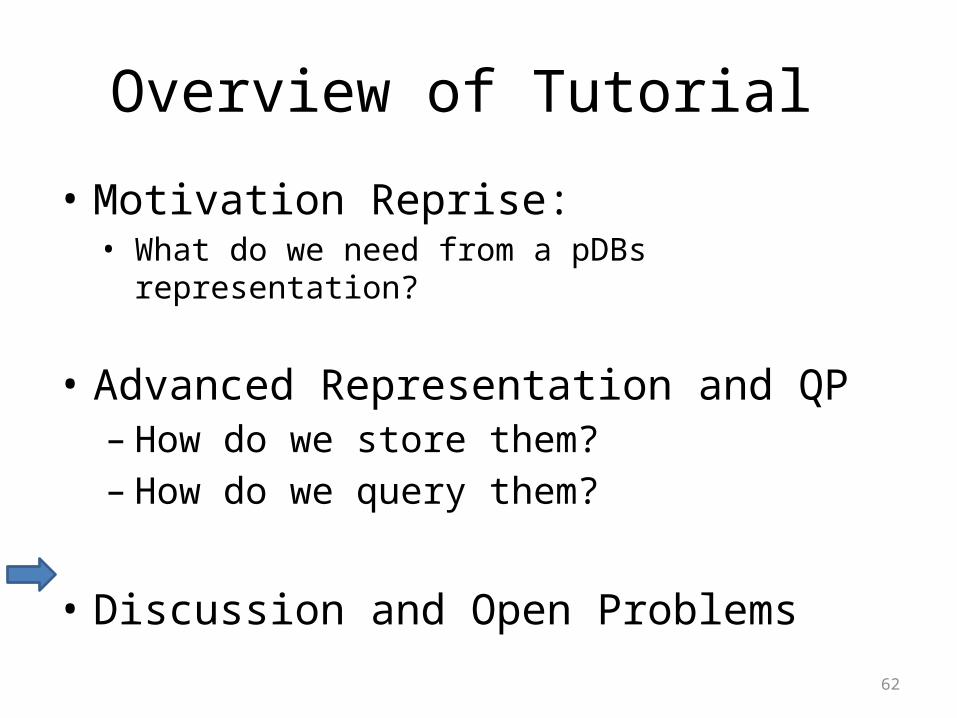
Overview of Tutorial

• Motivation Reprise: • What do we need from a pDBs representation?

• Advanced Representation and QP– How do we store them?– How do we query them?


63

Open Problems

– Challenges– Community– Language– Algorithmic

There are many more. Enumerate them in the community.

If you want to elaborate, please do!

64

Community Challenges

– Datasets for Uncertain Data– RFID ecosystem data released soon– http://MStreams.cs.washington.edu– IMDB data limited release

– Avoid pDBs being seen as “bad AI”– Need to clearly identify our space.

Make a solid business case

Export techniques, systems to other communities?Practice: Scale -- Theory: Data complexity

65

Model Challenges

– How to choose right level of correlations to model?– Too many, QP expensive– Too few, low answer quality

– How do we measure result quality?– Discussed by Cheng et al. ’03

Need a principled way to decide for DB apps

66

Language Challenges

– Management of lineage/provenance/trust– Trust issues can cause uncertainty

– Users want to take action– Is Hypothesis testing new decision support?

– What-if analysis– Explore how answers change via updates

Due to Koch: Need usecases for a languages w. uncertainty.

67

Algorithmic Challenges

– Indexing for Probabilistic Data– Can we compress, index or store probs on disk?

• [Letchner,R,B 08] [Das Sarma et al 08] [Singh et al 08]

– Combine discrete and continuous techniques– Updates: How to deal with changes in the

probability model efficiently?

– Mining uncertain data [Cormode and McGregor 08]

68

Day Two Takeaways

– Taxonomy for pDBs based on (a) type of data (b) type of correlations

– Saw three common techniques for scale: 1. intensional processing2. independence3. Reuse/Memoization

Tell our story to the larger CS community

Get involved, lots of interesting work!

69

Thank You

System Aspects of Probabilistic DBs Part II: Advanced Topics Magdalena Balazinska, Christopher Re...

Documents

Transcript of System Aspects of Probabilistic DBs Part II: Advanced Topics Magdalena Balazinska, Christopher Re...