System and Boundary Conceptualization in Ground-Water Flow Simulation

System and BoundaryConceptualization inGround-Water FlowSimulation

U.S. Department of the InteriorU.S. Geological Survey

Techniques of Water-Resources Investigationsof the United States Geological Survey

Book 3Applications of Hydraulics

Chapter B8

Availability of Publications of the U.S. Geological Survey

Order U.S. Geological Survey (USGS) publications by calling the toll-free telephone number 1-888-ASK-USGS or contact-ing the of ces listed belo w. Detailed ordering instructions, along with prices of the last offerings, are given in the cur-rent-year issues of the catalog “New Publications of the U.S. Geological Survey.”

Books, Maps, and Other Publications

By Mail

Books, maps, and other publications are available by mail from—

USGS Information ServicesBox 25286, Federal CenterDenver, CO 80225

Publications include Professional Papers, Bulletins, Water- Supply Papers, Techniques of Water-Resources Investigations, Circulars, Fact Sheets, publications of general interest, single copies of permanent USGS catalogs, and topographic and thematic maps.

Over the Counter

Books, maps, and other publications of the U.S. Geological Survey are available over the counter at the following USGS Earth Science Information Centers (ESIC’s), all of which are authorized agents of the Superintendent of Documents:

• Anchorage, Alaska—Rm. 101, 4230 University Dr.• Denver, Colorado—Bldg. 810, Federal Center• Menlo Park, California—Rm. 3128, Bldg. 3,

345 Middle eld Rd.• Reston, Virginia—Rm. 1C402, USGS National Center,

12201 Sunrise Valley Dr.• Salt Lake City, Utah—2222 West, 2300 South• Spokane, Washington—Rm. 135, U.S. Post Of ce

Building, 904 West Riverside Ave.• Washington, D.C.—Rm. 2650, Main Interior Bldg.,

18th and C Sts., NW.

Maps only may be purchased over the counter at the following USGS of ce:

• Rolla, Missouri—1400 Independence Rd.

Electronically

Some USGS publications, including the catalog “New Publica-tions of the U.S. Geological Survey,” are also available elec-tronically on the USGS’ s World Wide Web home page athttp://www.usgs.gov

Preliminary Determination of Epicenters

Subscriptions to the periodical “Preliminary Determination of Epicenters” can be obtained only from the Superintendent of

Documents. Check or money order must be payable to the Superintendent of Documents. Order by mail from—

Superintendent of DocumentsGovernment Printing Of ceWashington, DC 20402

Information Periodicals

Many Information Periodicals products are available through the systems or formats listed below:

Printed Products

Printed copies of the Minerals Yearbook and the Mineral Com-modity Summaries can be ordered from the Superintendent of Documents, Government Printing Of ce (address abo ve). Printed copies of Metal Industry Indicators and Mineral Indus-try Surveys can be ordered from the Center for Disease Control and Prevention, National Institute for Occupational Safety and Health, Pittsburgh Research Center, P.O. Box 18070, Pitts-burgh, PA 15236–0070.

Mines FaxBack: Return fax service

1. Use the touch-tone handset attached to your fax machine’s telephone jack. (ISDN [digital] telephones cannot be used with fax machines.)2. Dial (703) 648–4999.3. Listen to the menu options and punch in the number of your selection, using the touch-tone telephone.4. After completing your selection, press the start button on your fax machine.

CD-ROM

A disc containing chapters of the Minerals Yearbook (1993–95), the Mineral Commodity Summaries (1995–97), a statisti-cal compendium (1970–90), and other publications is updated three times a year and sold by the Superintendent of Docu-ments, Government Printing Of ce (address abo ve).

World Wide Web

Minerals information is available electronically athttp://minerals.er.usgs.gov/minerals/

Subscription to the catalog “New Publications of the U.S. Geological Survey”

Those wishing to be placed on a free subscription list for the catalog “New Publications of the U.S. Geological Survey” should write to—

U.S. Geological Survey903 National CenterReston, VA 20192

Contents I

Techniques of Water-Resources Investigations of the U.S. Geological SurveyBook 3, Applications of HydraulicsChapter B8

System and Boundary Conceptualizationin Ground-Water Flow Simulation

By Thomas E. Reilly

II Contents

U.S. DEPARTMENT OF THE INTERIOR

GALE A. NORTON, Secretary

U.S. GEOLOGICAL SURVEY

Charles G. Groat, Director

Reston, Virginia 2001

ISBN 0-607-96648-3

For sale by U.S. Geological SurveyBranch of Information ServicesBox 25286, Federal CenterDenver, CO 80225

Contents III

CONTENTSAbstract .......................................................................................................................................................................................... 1

Introduction ....................................................................................................................................................................................1

Selection and simulation of physical features of ground-water systems as boundaryconditions in ground-water flow models ........................................................................................................................................2

Streams ..................................................................................................................................................................................3

Lakes and reservoirs ..............................................................................................................................................................6

Wetlands ................................................................................................................................................................................7

Springs ...................................................................................................................................................................................7

Recharge at the water table ....................................................................................................................................................7

Earth materials of low hydraulic conductivity .......................................................................................................................9

Inter-basin flow ......................................................................................................................................................................9

Ground-water evapotranspiration ..........................................................................................................................................9

Spatial changes in density of water .....................................................................................................................................11

Ground-water divides ..........................................................................................................................................................12

Artificial boundaries that are not physical features .............................................................................................................14

Examples of the conceptualization of boundary conditions for two ground-water models .........................................................14

Conceptualization of the Albuquerque Basin, New Mexico ground-water flow system .....................................................14

Boundary conditions associated with physical features at the lateral extent of the model ........................................16

Boundary conditions associated with physical features at the bottom of the model ..................................................16

Boundary conditions associated with physical features at the top of the model ........................................................16

Water budget for the system .......................................................................................................................................16

Conceptualization of the Long Island, New York ground-water flow system .....................................................................19

Boundary conditions associated with physical features at the lateral extent of the model ........................................21

Boundary conditions associated with physical features at the bottom of the model ..................................................21

Boundary conditions associated with physical features at the top of the model ........................................................22

Water budget for the system .......................................................................................................................................22

Summary and Conclusions ...........................................................................................................................................................23

Acknowledgments ....................................................................................................................................................................... 23

Selected References .................................................................................................................................................................... 23

Appendix 1. List of “Packages” in the U.S. Geological Survey Modular Three-DimensionalGround-Water Flow Model (MODFLOW) used to represent physical features of aground-water system as mathematical boundary conditions ...............................................................................................26

Techniques of Water-Resources Investigations of the U.S. Geological Survey ..........................................................................27

FIGURES1. Flow chart of the ground-water flow modeling process ........................................................................................................... 2

2. Interactions of a stream and a ground-water system (Modified from Winter and others,1998): (A) gaining stream, (B) losing stream, and (C) losing stream separated from the saturatedground-water system ................................................................................................................................................................ 3

IV Contents

FIGURES–continued

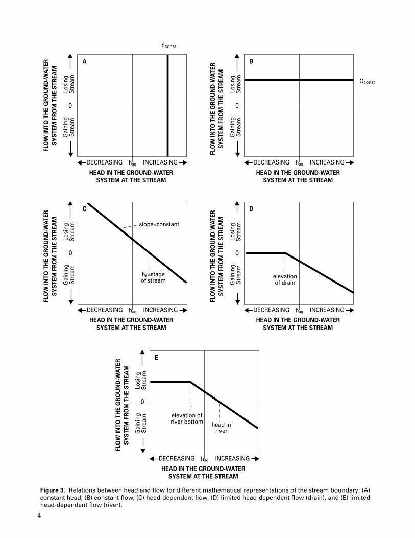
3. Relations between head and flow for different mathematical representations of thestream boundary: (A) constant head, (B) constant flow, (C) head-dependent flow,(D) limited head-dependent flow (drain), and (E) limited head-dependent flow (river) ..................................................... 4

4. Conceptual representation of a head-dependent flow or ‘leaky’ boundary condition as implementedin a finite-difference flow model (From McDonald and Harbaugh, 1988) ......................................................................... 5

5. Cross-sectional view of a finite-difference representation simulating a variable thicknessground-water system with flow to a specified head due to areal recharge:(A) Starting head set at 20 meters, and (B) Starting head set at 100 meters ....................................................................... 8

6. Diagram of a valley-fill aquifer system that is recharged by infiltration of surface runoff andlateral ground-water inflow from the surrounding bedrock ................................................................................................ 9

7. Location of the alluvial basins studied by the Southwestern Alluvial BasinsRegional Aquifer-Systems Analysis (Modified from Wilkins, 1998) ................................................................................ 10

8. Graph showing the simplified mathematical relation between the head in the aquifer andoutflow from the aquifer due to evapotranspiration as used in the ground-water flowmodel, MODFLOW........................................................................................................................................................... 11

9. A ground-water system containing fresh and salty water in acoastal environment (Modified from Reilly and Goodman, 1985) ................................................................................... 12

10. Diagrams showing generalized ground-water flow (A) under natural undisturbedconditions and (B) affected by pumping (From Grannemann and others, 2000) .............................................................. 12

11. Head distribution for a hypothetical ground-water system consistingof two streams separated by a ground-water divide .......................................................................................................... 13

12. Head distribution: (A) for the full hypothetical ground-water systemconsisting of two streams separated by a ground-water divide, and (B) for a similarground-water system in which a no-flow boundary is simulated at the initial ground-waterdivide resulting in half of the original system being used to simulate the system. In bothsystems, one well is discharging at a rate of 2,447 m3/d ................................................................................................... 13

13-16. Maps showing:13. Location of the Albuquerque Basin, central New Mexico (Modified from Bartolino, 1999) ............................... 1514. Simulated steady-state head in model layer 1 of the Albuquerque Basin model (Modified from Kernodle and others, 1995) .............................................................................................. 1715. Estimated mountain-front and tributary recharge to the Albuquerque Basin, and inflow from adjacent basins (Modified from Kernodle and others, 1995) ........................................................... 1816. Location of Long Island, New York (From Buxton and Smolensky, 1999) .......................................................... 20

17. Hydrogeologic section of Long Island, New York (From Buxton and Smolensky, 1999) ................................................ 20

18. Areal representation of Long Island, New York, by the regional ground-water flow model:(A) Actual map view; and (B) Discretized map view (From Buxton and Smolensky, 1999) ........................................... 21

19. Cross-sectional representation of the ground-water flow system, Long Island, New York,in the regional ground-water flow model: (A) Actual cross section; and(B) Discretized cross section. Section located near A-A’ in figure 18 (From Buxton and others, 1999) .......................... 22

Contents V

TABLES1. Common designations for the three common mathematical boundary conditions

specified in mathematical analyses of ground-water flow systems(Modified from Franke and others, 1987)[h is head (L), n is directional coordinate normal to the boundary (L)] .............................................................................. 1

2. Heads calculated for the same hypothetical ground-water flow system with arealrecharge and two different initial heads ............................................................................................................................... 9

3. Simulated annual water budgets for the Albuquerque Basin for predevelopmentand 1994 (Modified from Kernodle and others, 1995). [All values are in acre-feet per year] .......................................... 19

4. Simulated annual water budgets for the Long Island, New York ground-water systemfor predevelopment and the period of 1968-1983 (Modified from Buxton andSmolensky, 1999). [All values are in million gallons per day] ......................................................................................... 23

CONVERSION FACTORS

Multiply By To obtain

Metric units are used in all original work presented in this report. Two case studies are presented at the end

of the report, however, that are based on previously published reports. The system of units that were

originally used in these case studies are retained here in order not to introduce any round-off errors and to

show the level of approximation used in the investigator’s estimates.

foot (ft) 0.3048 meter (m)

mile (mi) 1.609 kilometer (km)

square mile (mi2) 2.590 square kilometer (km2)

cubic foot per second (ft3/s) 0.02832 cubic meter per second (m3/s)

acre-foot (acre-ft) 4.356 x 104 cubic feet (ft3)

acre-foot (acre-ft) 3.259 x 105 gallons (gal)

VI Contents

1

ABSTRACTGround-water models attempt to represent an actual

ground-water system with a mathematical counterpart. Theconceptualization of how and where water originates in theground-water-flow system and how and where it leaves thesystem is critical to the development of an accurate model.The mathematical representation of these boundaries in themodel is important because many hydrologic boundary con-ditions can be mathematically represented in more than oneway. The determination of which mathematical representa-tion of a boundary condition is best usually is dependentupon the objectives of the study. This report focuses on thespecific aspect of describing different ways to simulate, in anumerical model, the physical features that act as hydrologicboundaries in an actual ground-water system. The ramifica-tions, benefits, and limitations of each approach are enumer-ated, and descriptions of the representation of boundaries inmodels for Long Island, New York, and the Middle RioGrande Basin, New Mexico, illustrate the application ofsome of the methods.

INTRODUCTIONDuring the past several decades, computer simulation

models for analyzing flow and solute transport in ground-wa-ter and surface-water systems have played an increasinglyimportant role in the evaluation of alternative approaches toground-water development and management. The use ofthese models has somewhat paralleled the widespread use ofcomputers in today’s society. Ground-water models (for ex-ample, McDonald and Harbaugh, 1988) attempt to representthe actual ground-water system with a mathematical counter-part. The underlying philosophy of the simulation approachis that an understanding of the basic laws of physics and anaccurate description of the specific system under study willenable an accurate quantitative understanding of the causeand effect relationships. This quantitative understanding ofthese relationships enables forecasts to be made for any de-fined set of conditions, even those outside the range of ob-served conditions. Because of the uncertainties due to sparseor inaccurate data, poor definition of stresses, and errors inthe scientists’ deductive reasoning process, however, preciseforecasts of future events will rarely be a reality for ground-water systems (see Konikow and Bredehoeft, 1992). Eventhough forecasts of future events based on models (if devel-oped competently and objectively) are imprecise, they repre-sent the best available decision making information at thetime the forecasts are made.

Models that accurately represent the ground-water sys-tem being evaluated are expected to produce more accurateforecasts than those models that fail to represent important

aspects of the system. The determination of which aspects ofan actual ground-water system should be incorporated into acomputer simulation usually depends, in part, upon the ob-jectives of the study for which the model is being developed.The objectives of a study influence the size of the area of in-terest, the depth of concern, the scale of discretization (sizeof the model blocks or elements), and the method used torepresent the boundary conditions of the model domain.

Computer simulations of ground-water flow systems nu-merically evaluate the mathematical equation governing theflow of fluids through porous media. This equation is a sec-ond-order partial differential equation with head as the de-pendent variable. In order to determine a unique solution ofsuch a mathematical problem, it is necessary to specifyboundary conditions around the flow domain for head (thedependent variable) or its derivatives (Collins, 1961). Thesemathematical problems are referred to as boundary-valueproblems. Thus, a requirement for the solution of the math-ematical equation that describes ground-water flow is thatboundary conditions must be prescribed over the boundary ofthe domain. Three types of boundary conditions – specifiedhead, specified flow, and head-dependent flow – are com-monly specified in mathematical analyses of ground-waterflow systems (table 1). The values of head (the dependentfunction) in the flow domain must satisfy the pre-assignedboundary conditions to be a valid solution.

To obtain a solution to the ground-water flow equation,it is a mathematical requirement that boundary conditions bespecified along the entire boundary of the three-dimensionalflow domain. In solving a ground-water flow problem, how-ever, the boundary conditions are not simply mathematicalconstraints; they generally represent the sources and sinks of

By Thomas E. Reilly

Boundary typeand name

FormalName

Mathematicaldesignation

Type 1Specified head Dirichlet h (x,y,z,t) = constant

= constant

= constant

Type 2Specified flow

Neumann

Type 3Head-dependent flow

Cauchy(where c is also a constant)

dndh (x,y,z,t)

+ chdndh

Table 1. Common designations for the three commonmathematical boundary conditions specified in mathema-tical analyses of ground-water flow systems (Modifiedfrom Franke and others, 1987)[h is head (L), n is directional coordinate normal to theboundary (L)]

System and Boundary Conceptualizationin Ground-Water Flow Simulation

2

water within the system. Furthermore, their selection is criti-cal to the development of an accurate model (Franke and oth-ers, 1987). Not only is the location of the boundaries impor-tant, but also their numerical or mathematical representationin the model. This is because many physical features that arehydrologic boundaries can be mathematically represented inmore than one way. The determination of which mathemati-cal representation of a boundary condition is best usually isdependent upon the objectives of the study. A model of a par-ticular area developed for one study with a particular set ofobjectives may not necessarily be appropriate for another

study in the same area, but with different objectives.Many reports and books have discussed the role and use

of models in the analysis of ground-water problems (for ex-ample, Anderson and Woessner, 1992). Ground-water flowmodels attempt to represent the essential features and opera-tion of the actual ground-water system by means of a math-ematical counterpart. Figure 1 outlines some of the typicalsteps in the modeling process. One specific but very impor-tant component of the modeling process is the conceptualiza-tion and selection of boundary conditions, which is includedas part of the second step called ‘Develop ConceptualModel’ in figure 1. Another important component is themathematical approximation of hydrologic boundaries,which is included in the third step called ‘Develop Math-ematical Model’ in figure 1.

Although some investigators have documented and ex-plained the mathematical boundary conditions used inground-water flow models (for example, Franke and others,1987), most approach the topic from the applied mathemati-cal perspective, which is based on the mathematical bound-ary types listed in table 1. This report attempts to use aphysically based approach, using the physical features of theboundary surrounding the ground-water system as the focalpoint. The purpose of this report, then, is to focus on the spe-cific aspect of boundary conditions in the modeling processby describing the different ways of simulating, in a numeri-cal model, the physical features that are boundaries of theground-water system, and to discuss the ramifications, ben-efits, and limitations of each approach. Careful conceptual-ization of the hydrologic system under study and a consciousselection of the best mathematical, or model, representationof the physical features that are hydrologic boundaries is akey to the development of reasonably accurate simulations.

SELECTION AND SIMULATION OF PHYSICAL FEA-TURES OF GROUND-WATER SYSTEMS AS BOUNDARYCONDITIONS IN GROUND-WATER FLOW MODELS

In the ground-water flow modeling process (fig. 1),boundary conditions have an important influence on the ex-tent of the flow domain to be analyzed or simulated. In theproblem definition stage, the extent of the flow domain is ini-tially determined by the areal extent of the area of concern.In developing a conceptual model, the extent of the flow do-main to be analyzed is expanded vertically and horizontallyto coincide with physical features of the ground-water sys-tem that can be represented as boundaries. The effect of theseboundaries on heads and flows must then be conceptualized,and the best or most appropriate mathematical representationof this effect is selected for use in the model. The key is toselect the boundary of the model to coincide with a feature inthe actual system that can be simulated reasonably well andthat will minimize the effect of any artificial approximation.During the simulation process, the extent of the model, theconceptualization of the flow system, and mathematical rep-resentation of the boundaries is continually checked andevaluated to ensure the representation of the system capturesthe essence of the actual ground-water system.

THE MODELING PROCESS

Define Problem• Literature Review

• Preliminary Analyses

• Data Collection

Develop Conceptual Model• Processes

• Boundary Conditions

• Hydrogeology

• Data Collection

Develop Mathematical Model• Differential Equations

• Analytical Methods

• Numerical Methods

Assessment of ProblemUsing Model

Apply Results

Re-evaluation of the Problem andObjectives in light of the

Simulation Results

Calibration• History Matching

• Sensitivity Analyses

• Data Collection

Completion of Project

Figure 1. Flow chart of the ground-water flow mod-eling process.

3

A thorough understanding of hydrologic boundaries innature and the different ways to simulate them is required toselect the best mathematic representation in a ground-waterflow model. The objective of the modeling analysis and themagnitude of the stresses to be simulated also influence theselection of the appropriate approach to simulate the physicalfeatures that bound the ground-water system. When ground-water systems are heavily stressed, the physical features thatbound the system can change in response to the stress. Anyrepresentation of these features must account for these poten-tial changes, either by understanding the limitations of thesimulation or by representing the physical feature as realisti-cally as possible.

This section of the report describes the various types ofhydrologic boundaries that can affect ground-water flow sys-tems. The different approaches that can be taken to simulateeach physical feature are enumerated. The possible effects ofeach physical feature as a boundary on the flow system andthe ramifications and limitations of the different approachesare discussed.

StreamsStreams are surface features that commonly form a

boundary of the saturated ground-water flow system.Streams are important boundaries of ground-water systemsbecause they influence the heads and flows of the ground-water system with which they interact. Streams can gainwater from the ground-water system (fig. 2A) or lose waterto the ground-water system (fig. 2B). Losing streams can beconnected to the ground-water system by a continuous satu-rated zone (fig. 2B) or can be disconnected from the ground-water system by an unsaturated zone (fig. 2C). Some stream-beds consist of material of low hydraulic conductivity thatcan cause a large head difference between the stream and theaquifer, while other streams may be well connected to theaquifer system through permeable material of high hydraulicconductivity. Some streams are deeply incised into the aqui-fer whereas others may not be.

Just as there are many types of streams, there are manyways to represent a stream in a numerical model. Each waytreats the interaction of the stream with the ground-watersystem differently. These different conceptualizations mayproduce the same results under some conditions and very dif-ferent results under other conditions or stresses.

In ground-water models, a stream may be representedas:1. A specified-head boundary (also known as a Type 1 or

Dirichlet boundary)2. A specified-flow boundary (also known as a Type 2 or

Neumann boundary)3. A head-dependent or ‘leaky’ boundary (also known as a

Type 3 or Cauchy boundary)4. Nonlinear variations of the ‘leaky’ boundary:

a. A strictly gaining stream (a drain)b. A stream with a constant stage that can become disconnected from the saturated zone

c. A stream whose stage is calculated as part of the model solution.The level of complexity and data required varies for the

different approaches. Each approach is valid for specificconceptualizations, and it is important that the type ofboundary selected be consistent with the actual system, theobjectives of the study, and the intended use of the model.

When a stream is represented as a specified-head bound-ary, nodes in the model, where the stream is located, aresimulated with a head that is unchanging. This head, usually,is set at the stage of the stream. It implies that there is nohead loss between the stream and the ground-water systemand that the flow of ground water into or from the streamwill not affect the stage of the stream (fig. 3A). The amountof water flowing between the stream and the ground-watersystem then depends upon the ground-water heads in the

GAINING STREAM

Flow direction

Water table UnsaturatedZone

Saturated zone

A

LOSING STREAM

Flow direction

Water table

StreambedUnsaturated

zone

B

C

LOSING STREAM THAT IS DISCONNECTEDFROM THE WATER TABLE

Flow direction

Water table

Unsaturatedzone

Streambed

Streambed

Figure 2. Interactions of a stream and a ground-watersystem (Modified from Winter and others, 1998): (A)gaining stream, (B) losing stream, and (C) losing streamseparated from the saturated ground-water system.

4

AG

aini

ngS

trea

mLo

sing

Str

eam

0

DECREASING

HEAD IN THE GROUND-WATER

SYSTEM AT THE STREAM

INCREASINGhaq

B

Gai

ning

Str

eam

Losi

ngS

trea

m

FLO

W IN

TO

TH

E G

RO

UN

D-W

AT

ER

SY

ST

EM

FR

OM

TH

E S

TR

EA

M

0

DECREASING



INCREASINGhaq

hconst

Qconst

D

Gai

ning

Str

eam

Losi

ngS

trea

m

FLO

W IN

TO

TH

E G

RO

UN

D-W

AT

ER

SY

ST

EM

FR

OM

TH

E S

TR

EA

M

0

DECREASING



INCREASINGhaq

C

Gai

ning

Str

eam

Losi

ngS

trea

m

FLO

W IN

TO

TH

E G

RO

UN

D-W

AT

ER

SY

ST

EM

FR

OM

TH

E S

TR

EA

M

FLO

W IN

TO

TH

E G

RO

UN

D-W

AT

ER

SY

ST

EM

FR

OM

TH

E S

TR

EA

M

0

DECREASING



INCREASINGhaq

E

Gai

ning

Str

eam

Losi

ngS

trea

m

FLO

W IN

TO

TH

E G

RO

UN

D-W

AT

ER

SY

ST

EM

FR

OM

TH

E S

TR

EA

M

0

DECREASING



INCREASINGhaq

elevationof drain

elevation ofriver bottom head in

river

hs=stageof stream

slope=constant

Figure 3. Relations between head and flow for different mathematical representations of the stream boundary: (A)constant head, (B) constant flow, (C) head-dependent flow, (D) limited head-dependent flow (drain), and (E) limitedhead-dependent flow (river).

5

nodes that surround the specified-head boundary represent-ing the stream. This representation may be appropriate forlarge streams or for systems in which the stream is well con-nected to the ground-water system and the stream stage is notexpected to change.

A stream can be simulated as a specified flow boundaryif the loss or gain rate of the stream is known. This boundaryis simulated by specifying a flow rate at a node or locationrepresenting the stream. In this representation, the flow rateis independent of the head in the aquifer (fig. 3B). This rep-resentation may be appropriate for streams that are discon-nected from the ground-water system, such as streams athigh altitudes that lose their water as they enter the valley de-posits from the mountains. It also may be appropriate forsome steady-state simulations of conditions in which thestream interaction has been well measured and no changes instress will be simulated. Conceptually, representing thestream as a specified flow assumes that the flow of water be-tween the ground water and the stream is independent of theheads in the ground-water system (fig. 3B) and the surface-water system.

A stream can be simulated as a head-dependent flow or‘leaky’ boundary, which is also referred to as a ‘general headboundary’ in the finite-difference model MODFLOW(McDonald and Harbaugh, 1988). This boundary representsthe stream as having a constant specified stage, but a layer ofmaterial (the streambed) or some other resistance is presentbetween the stream and the ground-water system (fig. 4).This representation assumes that the stream and the ground-water system are always connected, and the flow from or tothe stream is directly proportional to the head difference be-tween the stream stage and the head in the ground-water sys-tem (fig. 3C).

The first three possible representations of a stream areall linear in that the stage in the stream and the equation rep-resenting the flow between the aquifer and the stream do notchange as a function of the head in the ground-water system.Thus, these representations can be used in modelconceptualizations that employ superposition (Reilly andothers, 1987). The three remaining ways to represent astream in a ground-water flow model are nonlinear varia-tions of the ‘leaky’ boundary in that the coefficients of theequation used or the stage of the stream depends directly onthe head in the aquifer.

The first representation, and perhaps the simplest of thenonlinear representations, is for the case of a strictly gainingstream. This case is simulated by use of the ‘drain’ packagein MODFLOW (McDonald and Harbaugh, 1988). In thisconceptualization, the only source of water to the stream ordrain is that which enters the stream or drain as ground-wa-ter inflow. If the head in the ground-water system falls be-low the altitude of the stream or drain bottom, the ground-water inflow to the stream or drain ceases and the streamdries up (fig. 3D). This conceptualization is useful in simu-lating ground-water drains or headwater streams that havevery little surface runoff relative to ground-water inflow.The representation of streams as a drain must be used cau-tiously, however, because each node represented as a drain

is independent of all the other nodes represented as a drain. Ifa stream represented as a drain goes dry in the middle of itsreach, it cannot represent the fact that water that is in thestream upstream from the dry section could infiltrate in thedry stream and provide flow from the stream to the aquifer.Thus, as with all boundary conceptualizations, the use of thisconceptualization of a stream must be consistent with howthe stream functions in nature.

The second representation (fig. 3E) is an extension ofthe ‘leaky’ boundary condition in that it also allows the headin the ground-water system to be below the stream bottom(fig. 2C). This case, for the condition in which the stream be-comes disconnected from the ground-water system, is simu-lated as a condition of a fixed flow. When the stream be-comes disconnected from the saturated ground-water system,the flow leaving the stream is independent of the head in theground-water system. This representation assumes that thestage in the stream is specified and is not a function of theamount of ground-water inflow or outflow. Thus, the streamcan never go dry regardless of how much water is lost to theground-water system. When using this representation, the in-vestigator must carefully examine the water budget of thesystem and of the boundary to ensure that the quantities ofwater being simulated in the model are plausible in the actualsystem.

The last representation is the most complex and can beimplemented by many different means. For this last represen-tation, a model of the stream system is coupled to the modelof the ground-water system. In this approach, the stage of thestream is dependent upon the amount of flow in the streamand the amount of flow between the ground-water systemand the stream. Existing models of stream systems are nu-merous and are based on different methods and levels ofcomplexity. Three different methods for simulating a streamsystem have been implemented in the ground-water modelMODFLOW. These are the stream-flow routing package(Prudic, 1989), DAFLOW-MODFLOW (Jobson andHarbaugh, 1999), and MODBRANCH (Swain and Wexler,1993). These methods may represent the system accurately,but the information and data needs increase and the numeri-

hi,j,k

hbi,j,k

Qbi,j,k

Conductance,Cbi,j,k

betweensource and

cell i,j,k

Cell i,j,k Constant-head

Source

Figure 4. Conceptual representation of a head-dependent flow or ‘leaky’ boundary conditionas implemented in a finite-difference flowmodel. (From McDonald and Harbaugh, 1988)

6

cal methods may lose stability for the more complex streamsimulation packages. The response times for flow in streamsis usually significantly faster than response times for ground-water systems and this incongruity can cause problems in de-termining an appropriate simulation strategy. This couplingof ground-water and surface-water models is needed wherethe short-term fluctuations in the ground-water system due tothe influence of the surface water are important to the objec-tives of the study. The coupling of ground-water and surface-water models is also necessary if the stream may dry up orrewet during the course of the simulation. In cases in whichthis level of detail is not needed, the simpler methods canprovide equivalent model results.

In model design, selection of the appropriate mathemati-cal boundary condition to represent a particular stream in ahydrologic system is a key decision that can affect the abilityof a model to make accurate forecasts. Considerations thatmust enter into the selection are the nature of the stream (forexample, flow rate, variability of the flow, type of streambed,connection with the ground-water system), the objectives ofthe study, and the potential uses of the model. In methodsthat do not keep track of the amount of water in the stream,there are no constraints on the amount of water availablefrom the stream. As pumping rates increase in such a system,an unrealistic amount of water may be induced to flow fromthe stream to the ground-water system. This means that themodel user must check to see if the amount of water beingsupplied from the boundary (stream) is reasonable. For ex-ample, the simulated amount of water being supplied by thestream to the ground-water system should not exceed the to-tal amount of streamflow available. Thus, the magnitude ofthe stress imposed on the system can affect the validity of theboundary condition. A model developed for one set of condi-tions may not be valid when applied to a different, more ex-treme set of conditions. The conceptualization of the interac-tion between the surface-water system and the ground-watersystem is very important and must be continually evaluatedduring the use of the model.

Lakes and ReservoirsLakes and reservoirs are usually hydraulically connected

to ground-water flow systems and can be significant physicalfeatures of the flow system. The manner in which they arerepresented in a numerical model is important to accuratelyreproduce their role in the actual ground-water system. Theirrole is similar to that of streams in that lakes and reservoirscan lose water to the ground-water system, gain water fromthe ground-water system, or do both. In some situations,lakes and reservoirs can be simulated with the same bound-ary conditions as those used for streams. In some instances,however, where the lake or reservoir level and area are de-pendent upon the interaction with ground water, a more com-plex approach is required.

In ground-water models, a lake or reservoir may be rep-resented as:1. A specified-head boundary2. A head-dependent or ‘leaky’ boundary

3. Nonlinear variations of the ‘leaky’ boundary:a. A lake or reservoir with a constant stage that can be-come disconnected from the saturated zoneb. A lake or reservoir whose stage and area is problem de-pendent and is calculated as part of the model solution.

4. A volume of material of high hydraulic conductivity withrecharge calculated as areal precipitation minus lakeevaporation. (This is not strictly a boundary condition;rather it is an approach to simulate the effect of the lake.)

As with the simulation of streams, the appropriatemethod to simulate a lake or reservoir depends upon thecharacteristics of the lake or reservoir in nature (for example,size, stage variation, type of lake-bed sediments, sources ofwater) and the expected stresses to be imposed on the model(that is, the objectives of the study using the model).

For cases in which the lake or reservoir is large and nochange in stage is expected for the stresses to be imposed onthe model, the specified-head and head-dependent boundaryconditions may be appropriate. As an example of this ap-proach, Eberts and George (2000) represented Lake Erie as aspecified-head boundary in their model of regional ground-water flow in the Midwestern Basins and Arches AquiferSystem of Indiana, Ohio, Michigan, and Illinois. If the stageof the lake is dependent on the heads and flows in theground-water system, however, then a different approach isrequired. For lakes with surface-water inflows and outflows,a model of the lake stage or lake area may be required. Asexamples of this approach, Cheng and Anderson (1993) useda formulation that calculated the lake stage as part of themodel, Fenske and others (1996) used a formulation that cal-culated a changing area of infiltration for reservoirs forwhich the stage was prescribed over time, and Merritt andKonikow (2000) used a formulation that calculates both thestage and area of the lake as part of the model solution. Forlakes that are basically surface expressions of the ground wa-ter system, the lake can be simulated as a volume of materialof very high hydraulic conductivity with the recharge set atprecipitation minus lake evaporation and a storage coefficientset at 1.0, as was implemented by Masterson and Barlow(1997) on Cape Cod, Mass.

A key to selecting the appropriate model representationof a lake or reservoir is to determine if the stresses to be ana-lyzed during the model analysis will affect the stage (waterlevel) in the lake or reservoir. If the stage will not be af-fected, then the simpler boundaries will suffice. The devel-oper or user of the model must check this assumption byevaluating the changes in flow between the lake and theground-water system to ensure that they can happen in theactual system without changes in stage occurring. For ex-ample, in a stressed system, if the flow from a lake into theground-water system is larger than the amount of water flow-ing into the lake and recharging the lake, the lake level in theactual system cannot be supported and will have to change.These examples again point out that a model of a specificsystem is constructed by selecting boundary conditions basedon certain assumptions regarding the use of the model, theamount of stress that will be simulated, and the accuracy re-

7

quired. If the model is used to evaluate conditions that nolonger are the same as the design assumptions, the resultswill be invalid. It is important for the analyst to constantlyevaluate the appropriateness of the methods used to simulatethe boundary conditions during the use of the model.

WetlandsWetlands are present wherever topography and climate

favor the accumulation or retention of water on the land-scape. Wetlands occur in widely diverse settings, fromcoastal margins to flood plains to mountain valleys. Similarto streams, lakes, and reservoirs, wetlands can receiveground-water inflow, recharge ground water, or do both. Amathematical representation of a wetland would be the sameor similar to the choices available for streams, lakes, and res-ervoirs. For example, Koreny and others (1999) represented awetland that was known to recharge the underlying ground-water system as a specified inflow boundary. Winston (1996)used the ‘drain’ conceptualization in MODFLOW to repre-sent a wetland that gained water from the ground-water sys-tem as a solely gaining discharge location. Swain and others(1996) used the MODFLOW/BRANCH model (Swain andWexler, 1993) to represent wetlands in southern DadeCounty, Fla. as a highly permeable layer coupled to a sur-face-water model. The best representation should be basedon an understanding of the source of water in the wetlandand the factors that regulate the exchange of water betweenthe ground-water system and the wetland. These factors arethe same as those for streams, lakes, and reservoirs, and aredescribed in the previous sections.

SpringsSprings typically are present where the water table inter-

sects the land surface. Springs represent a discharge from theground-water system. When the head in the aquifer becomeslower than the land surface opening of the spring, the springdries up. The higher the head in the aquifer above the altitudeof the spring opening, the more water discharges from thespring. Thus, springs are usually treated as nonlinear head-dependent discharge boundaries that have zero flow when thehead in the aquifer becomes lower than the altitude of thespring, using the same mathematical representation as thatused for a drain (fig. 3D).

Recharge at the Water TableRecharge is a term used to describe many of the pro-

cesses involved in the addition of water to the saturated zone(Wilson and Moore, 1998). This discussion will focus on re-charge at the water table from sources other than surface-water bodies.

Recharge from precipitation is frequently an importantsource of water to ground-water systems. In many if not mostlocations, precipitation (rainfall or snowmelt) soaks into theground and recharges the water table over the areal extent ofthe aquifer system. The amount of recharge is usually deter-mined externally to the model and is calculated as theamount of precipitation minus surface runoff and evapotrans-piration at land surface. The recharge rate is usually then in-

corporated into ground-water flow models as a specified-flow boundary condition along the top boundary of theground-water model. Although this approach is very straight-forward conceptually, several nuances must be consideredwhen implementing the simulation of areal recharge inground-water models.

One nuance is in selecting the best method to simulaterecharge in three-dimensional ground-water models in whichthe top surface of the saturated system (the water table) ex-tends into different model layers. The conceptual issue iswhether the recharge should enter only the top layer orshould enter the uppermost active layer. Usually, the rechargeis input to the uppermost active layer. How recharge occursin nature and how it is treated in any specific model must becarefully considered. The model MODFLOW provides op-tions that allow different approaches for simulating rechargeat the water table (McDonald and Harbaugh, 1988); someother models do not allow different conceptualizations andthe way in which these models treat the input of rechargemust be specifically considered to ensure accuracy.

Another nuance is not related to the physics of recharge,but rather to the numerical methods used in many ground-water models. In some unconfined ground-water systemswith areal recharge, the saturated zone becomes thinner nearthe lateral boundaries of the system. In simulating these sys-tems, models solving the nonlinear problem calculate thesaturated thickness as part of that solution. Because it is anonlinear problem in which the saturated thickness is a func-tion of the head, the solution techniques must iterate to ob-tain a solution. In iterating towards a solution, the heads may‘overshoot’ the correct head and cause a cell or areas of themodel to become incorrectly represented as dry, whichcauses the model cell or cells to be cut out of the activemodel area and made inactive. Under this condition, the arealrecharge that should be entering the system does not do sobecause the simulated lateral extent of the saturated systemhas been prematurely or incorrectly reduced. This causes themodel to account for a reduced amount of recharge, whichresults in an incorrect water budget and usually a truncatedmodel extent that would not exist in the actual system. Theonly way to detect this is to carefully evaluate the results ofany simulation and evaluate the extent and the amount of re-charge simulated.

If the model is not converging to the correct model ex-tent and amount of recharge, then non-standard approachesmust be employed to ensure that the boundary is reproducingthe actual system. Some of the approaches that investigatorshave used include: (1) reformulation to allow for the re-wet-ting of dry cells, (2) modification to parameters used in thesolution of the equations (the matrix solver), (3) a modifiedtransient approach, and (4) better starting heads for the ma-trix solution. The re-wetting approach is one that allows forinactive ‘dry’ cells to become active depending on the headsin the surrounding cells (for example, McDonald and others,1992). The re-wetting approach, however, is also subject tonumerical difficulties, and is not always a solution to theproblem. The approach of modifying solver parameters is

8

one whereby an attempt is made to slow down the conver-gence of the matrix problem in order to approach the correctsolution smoothly and not cause any cells to dry up prema-turely. Specifics of this approach depend on the matrix solu-tion technique used. The modified transient approach is onein which a steady-state solution is obtained by simulating theproblem as a transient condition and calculating the headsthrough time until they no longer change. This transient ap-proach slows down the rate of convergence so that the correctsolution is reached gradually through time. In steady-stateproblems, the use of starting heads that are close to the finalsolution can also remedy the problem. Some investigatorshave used fixed saturated thicknesses to simulate the problemand obtain an approximate solution; then, this approximateresultant head solution is used as starting heads for the non-linear water-table problem. With this technique, the equationsolver tends to oscillate less and approach the solutionsmoothly without making cells dry up incorrectly, becausethe starting heads are closer to the actual nonlinear solution.These approaches do not always work, however, and the in-vestigator is responsible to ensure that the solution is reason-able.

As an example of the discussionabove, consider a one-dimensional wa-ter-table system with a sloping imperme-able bottom that contains a specifiedhead and extends 5,000 meters, with anareal recharge rate of 0.5 m/yr. The start-ing head for the equation solution isspecified at 20 meters, which is above allthe bottom elevations of the cells but yetclose to the magnitude of the expectedresults. Figure 5A is a cross-sectionalview of a finite-difference representationof the steady-state solution. The cell far-thest from the specified head is simu-lated as being dry. The total rechargeflowing to the specified head cell for a500-meter width is 2,740 m3/d. The con-vergence criterion of the model was metand the mass balance was perfect. Nowconsider figure 5B, which is the result ofa simulation of the same problem, ex-cept the starting head for the matrix so-lution was set at 100 meters. As is shownin figure 5 and table 2, three cells arenow simulated as being dry. The result isthat less recharge is simulated as enter-ing the model and the heads and waterbudgets are reduced accordingly, withonly 2,055 m3/d being represented as re-charge entering the system for a 500-meter width. Although both solutionsconverged and had perfect mass bal-ances, at least one of them is incorrect.Because it is a nonlinear problem, it isnot easy to determine which is the cor-

rect solution. The rate of convergence and the method ofmaking cells inactive must be considered and evaluated. Afterevaluating these aspects, it seems that the first model is mostlikely correct. In the second model, the iterative solution, inattempting to converge, apparently overshot the bottom ofsome of the cells, which prematurely or erroneously truncatedthe area from the active model domain, and resulted in thewrong problem being solved. The model developer or usermust carefully evaluate nonlinear problems and monitor therate of convergence to ensure that cells that should be part ofthe active problem domain are not removed.

Recharge in valley-fill ground-water systems, particu-larly in arid areas, commonly originates from runoff fromsurrounding mountains or higher elevation locations (fig. 6).This runoff can be conceptualized as being either diffuse orchanneled. Diffuse runoff conceptualizes the process of sur-face runoff as occurring all along the boundary edge of themodeled ground-water system and the recharge is usuallysimulated as a specified-flow boundary along the top layer ofthe model. Channeled runoff conceptualizes the surface run-off as occurring in stream channels and the resultant ground-

ALT

ITU

DE

, IN

ME

TE

RS

-20

-10

0

0

0

10

20

-30

DISTANCE, IN METERS

DISTANCE, IN METERS

INACTIVE – DRY CELL

Altitude of cell bottom

Altitude of water table in cell

Specified head cell

5000

INACTIVE – DRY CELL

5000

A. Starting head set at 20 meters

B. Starting head set at 100 meters

ALT

ITU

DE

, IN

ME

TE

RS

-20

-10

0

10

20

-30

Figure 5. Cross-sectional view of a finite-difference representation simulat-ing a variable thickness ground-water system with flow to a specified headdue to areal recharge: (A) starting head set at 20 meters, and (B) startinghead set at 100 meters.

9

water recharge is usually simulated by means of a subset ofthe methods used to simulate streams, that is, either as aspecified-flow condition or by a nonlinear method such asstreamflow routing (Prudic, 1989). A potential additionalsource of recharge in valley systems is ground-water flowfrom the surrounding mountains. If the rocks of the moun-tains do contribute flow, that flow must be estimated andusually is conceptualized as a specified flow entering the val-ley-fill ground-water system along the boundary.

Earth Materials of Low Hydraulic ConductivityNo earth material is completely impervious to water.

Many earth materials, however, have very low hydraulic con-ductivities and thus contribute relatively small amounts ofwater to adjacent permeable ground-water systems. Depend-ing upon the conceptualization of the system and the objec-tives of the study, a boundary between a permeable ground-water system with appreciable flow and a surrounding bodyof earth material of low-hydraulic conductivity that contrib-utes a negligible amount of water commonly is treated as ano-flow boundary. This is a specified-flow boundary (table 1)across which the flow is exactly zero. For example, in the hy-pothetical valley-fill aquifer system shown in figure 6, if thebedrock contributes an insignificant amount of water to thevalley-fill deposits, the boundary of the valley-fill depositscould be conceptualized as an impermeable or ‘no-flow’boundary. This no-flow boundary is approximate becausesome flow probably enters the actual system across thisboundary. The objectives of the study and the relative magni-tudes of the flow in the bounding material, as compared tothe flow in the aquifer material, are key to assessing the as-sumption of negligible flow that can be approximated as noflow. In some systems, assuming a no-flow boundary may bereasonable for flow-system analysis, but such an assumptionmay not be appropriate for transport analysis in which the ac-tual path of a particle is important.

Inter-Basin FlowMany alluvial ground-water systems underlie major

river systems. These ground-water systems form sub-basinsalong the entire length of the river, for example, the alluvialbasins along the Rio Grande in New Mexico (Wilkins, 1998),as shown in figure 7. In an attempt to simulate flow in one ofthe sub-basins, the boundary that controls the exchange ofground water between adjacent basins can be important anddifficult to represent. As always, the key to a successfulsimulation effort is to select the boundary of the model to co-incide with a feature in the actual system that can be simu-lated reasonably well and that will minimize the effect of anyartificial approximation. This location is usually where thebasin narrows near the stream and is reasonably far from thearea to be stressed. Depending upon the situation, the bound-ary can be represented as a no-flow, specified-flow, speci-fied-head, or head-dependent flow boundary. None of thechoices are perfect because the actual ground-water systemdoes not begin or end at the boundary location, but is con-tinuous along the stream. Thus, any boundary condition to beused in a numerical ground-water flow model involves trade

offs that must be carefully evaluated on a case-by-case basisand monitored during the use of the model.

Ground-Water EvapotranspirationGround-water evapotranspiration is the process by

which water is removed from the saturated ground-water sys-tem by plant usage (transpiration) or evaporation. This is notto be confused with evapotranspiration at land surface or inthe unsaturated zone. Most ground-water models take intoaccount the rate of evapotranspiration at land surface and theunsaturated zone by subtracting it from the rate of precipita-tion in the calculation of a net recharge rate. How and wherein the saturated ground-water system evapotranspiration oc-curs should be thoroughly conceptualized to ensure that onlythe loss from the saturated zone is considered.

Some investigators have inadvertently ‘double counted’ground-water evapotranspiration by both removing it fromthe calculated areal recharge rate and simulating it in themodel, causing the system to be incorrectly represented. Anexample of ‘double counting’ and incorrectly applying

Bedrock

Boundaryground-waterinflow

Surface runoffrecharging the valleyat the boundary

Permeable valley-fillground-water system

Land Surface

Stream

Water Table

Figure 6. Diagram of a valley-fill aquifer system that is re-charged by infiltration of surface runoff and lateralground-water inflow from the surrounding bedrock.

Nodenumber

Head calculated with theinitial head at 20. m

Head calculated with theinitial head at 100. m

1 0.00 0.00

2 1.93 1.46

3 3.83 2.86

4 5.68 4.17

5 7.49 5.38

6 9.24 6.42

7 10.90 7.20

8 12.45 Dry

9 13.81 Dry

10 Dry Dry

Table 2. Heads calculated for the same hypotheticalground-water flow system with areal recharge and twodifferent initial heads.

10

Figure 7. Location of the alluvial basins studied by the Southwestern Alluvial Basins Regional Aquifer-Systems Analy-sis. The basins along the Rio Grande form a continuous stretch of alluvial deposits. (Modified from Wilkins, 1998)

1

2

4

5

6

7

8

9

10

14

18

15

16

17

12

13

1920

22

21

11

3

EXPLANATION

Area of basin fill—Indicates extent of basin fill within basin boundaries Province boundary

Basin boundary—Number and name listed below

San LuisEspañolaSanto DomingoAlbuquerque-BelenSocorroLa JenciaSan AgustinSan MarcialEnglePalomasJornada Del MuertoMesillaTularosa-HuecoMimbresHachitaPlayasAnimasLordsburgSaltEagleRedlight DrawPresidio

109° 108° 107° 106° 105°

38°

37°

36°

35°

34°

33°

32°

31°

30°

104°

MINERAL

SAGUACHE

RIOGRANDE

CONEJOS

NEW MEXICO

AR

IZO

NA

UT

AH

RIO ARRIBA

TAOS

SANDOVALMcKINLEY

CIBOLA

SANTA FE

TORRANCE

LINCOLNCATRON

OTERO

GRANT

HUDSPETH

CULBERSON

JEFF DAVIS

PRESIDIO

NEW MEXICOTEXAS

SAN JUAN

COLFAX

SAN MIGUEL

MORA

GUADALUPE

CHAVES

DEBACA

0 20 40 MILES

0 20 40 KILOMETERS

LOSALAMOS

VALENCIA

SIERRA

LUNA

EL PASO

MEXICOEl Paso

GREATPLAINS

PROVINCE

HIDALGO

UNITED STATES

Las Cruces

SOCORRO

BERNALILLO

Albuquerque

Jemez R.

COSTILLA

ALAMOSA

SOUTHERNROCKY

MOUNTAINPROVINCE

Co

nti

nen

talD

ivid

ean

d

approxim

atestu

dy-a

rea

boun

dar

y

Alamosa

COLORADO

NEWMEXICO

TEXAS

STUDYAREA

LOCATIONMAP

CUSTER

HUERFANO

PUEBLO

LASANIMAS

HINSDALE

MONTROSE

SAN MIGUEL

DOLORES

MONTEZUMA

LA PLATA

COLORADO

GUNNISON

SANJUAN

OURAY

ARCHULETA

FREMONT

App

roxi

mat

est

ud

y-ar

eabo

un

dar

y

BASIN ANDRANGE

PROVINCE

DONAANA

˜

REEVES

COLORADOPLATEAUSPROVINCE

ContinentalDivide

1. 2. 3. 4. 5. 6. 7. 8. 9. 10. 11. 12. 13. 14. 15. 16. 17. 18. 19. 20. 21. 22.

11

ground-water evapotranspiration is in cases in which the ar-eal recharge rate is calculated by means of hydrograph sepa-ration and ground-water evapotranspiration is included in thesimulations. Investigators use hydrograph separation to deter-mine the base flow of a stream, which represents the outflowfrom the ground-water system. Some investigators have thenequated the outflow of the system (the base flow) to the re-charge under unstressed conditions. The base flow, however,actually represents the areal recharge minus the water re-moved by ground-water evapotranspiration. Thus, theground-water evapotranspiration has already been taken intoaccount in the estimate of areal recharge and should not alsobe simulated in the numerical model. Conversely, if the loca-tion of the evapotranspiration is important and should besimulated in the model, then any estimate of recharge mustnot be based solely on the estimates of base flow. The physi-cal processes to be simulated must be carefully evaluated toensure that evapotranspiration is represented appropriately.

Ground-water evapotranspiration is usually conceptual-ized as occurring at a rate that varies with depth. It is assumedthat the nearer the water table is to the land surface, thegreater the likelihood that plant roots will be in direct contactwith the water table and the greater will be the amount ofwater withdrawn from the saturated zone. In MODFLOW,evapotranspiration is approximated as a linearly varying ratethat ranges from a maximum at elevations at or above landsurface and decreases to zero below some depth, referred toas an extinction depth (fig. 8). Because evapotranspirationloss from the saturated zone cannot be measured directly, thevarious conceptualizations are difficult to check indepen-dently. Most investigators realize that methods of accounting

for ground-water evapotranspiration in numerical models areusually a crude approximation of what actually occurs in na-ture. Because of the inability to compare simulated evapo-transpiration losses with measured losses, investigators mustrely on conceptualizations that are internally consistent andreasonable, although less than perfect.

Spatial Changes in Density of WaterThe density of the water moving through the ground-

water system is important in calculations of the fluid’s massbalance and its velocity. Numerical models that are designedto simulate ground-water flow usually assume a constantdensity for water and solve a mass balance equation withhead as the dependent variable. The amount of total dis-solved solids in the water and the temperature of the wateraffect the density of the water. To accurately account for theeffects of density on a flow system, a variable density flowand transport model is required, because the flow is depen-dent on the density distribution. There are, however, simpli-fied approaches to account for density variations in modelsthat are constructed primarily to simulate the movement ofthe fresh water in an environment that contains fresh waterand denser salt water (Reilly, 1993).

In systems in which the density changes abruptly be-tween a fresh water zone (or volume) and a more dense‘salty’ zone, the boundary between the fresh water and thesalt water can be conceptualized and approximated as a no-flow interface (fig. 9). The fresh water tends to flow alongand on top of the salty water and negligible flow crosses theinterface under equilibrium conditions. The interface can beapproximated as a zero specified flow (no flow) if the densitybetween the two fluids changes abruptly. The position of theboundary is dictated by the magnitude of the fresh-waterhead [see Reilly (1993) for a more detailed explanation]. Inconstant-density models, the location of the boundary can becalculated only under steady-state conditions or cases inwhich the movement of the boundary is assumed to be ofnegligible importance to the problem. In dual-density mod-els, where both the fresh-water zone and the salt-water zoneare simulated as two distinct systems, each with their ownconstant density [for example, the SHARP model by Essaid(1990)], the no-flow boundary between the two systems canmove transiently because the movement and storativity offluids in both systems are taken into account.

In layered coastal systems, such as that shown in figure9, the physical processes that occur in the confining unitmust also be conceptualized and the appropriate boundarycondition selected. Depending upon the hydraulic conductiv-ity, pressure, and density distributions, this boundary be-tween the fresh water and salt water at the confining unit canbe conceptualized as either a no-flow boundary or a head-de-pendent flow or ‘leaky’ boundary (Essaid, 1990; Reilly,1990). Conceivably, water can flow along the fresh water –salt water interface in the lower aquifer (fig. 9) and dischargeacross the confining unit into the salty ground water overly-ing the confining unit. In this conceptualization, the confin-ing unit would contain fresh water, the rate of discharge of

Altitude ofland surface

Flow

out

of a

quife

r 0

fl

ow in

to a

quife

r

decreasing haq increasing


SYSTEM AT THE WATER TABLE

FLO

W IN

TO

TH

E

GR

OU

ND

-WA

TE

R S

YS

TE

M

Altitude ofextinction depth

Figure 8. Graph showing the simplified mathematical re-lation between the head in the aquifer and outflow fromthe aquifer due to evapotranspiration as used in theground-water flow model, MODFLOW.

12

that fresh water into the overlying permeable zone of saltyground water would be small, and the fresh-water dischargewould not change the density of the overlying salty water be-cause it would mix thoroughly with the overlying water. In afresh-water simulation, the specified head at the head-depen-dent boundary would be the equivalent fresh-water head at

the top of the confining unit, and the dependent head wouldbe at the bottom of the confining unit and would be calcu-lated as part of the model solution. The confining unit is con-ceptualized as containing fresh water, and the calculation ofleakage, as illustrated in figure 4, would be a valid estimate,even in this two-density system. Obviously, this approach isan approximation, but it does mimic some of the coastal sys-tems observed in nature.

Ground-Water DividesA ground-water divide is not really a boundary in nature.

A ground-water divide is defined in the Glossary of Hydrol-ogy (Wilson and Moore, 1998) as: (a) a ridge in the watertable or other potentiometric surface from which the groundwater represented by that surface moves away in both direc-tions, and (b) the boundary between adjacent ground-waterbasins. Figure 10 shows a ground-water divide in an uncon-fined aquifer for natural undisturbed conditions (fig. 10A)and under stressed conditions (fig. 10B). Ground water oneach side of the divide moves away from the divide and noflow crosses the divide. When a system is pumped (stressed),the location of the divide can move in response to this pump-ing. Although a divide is a ridge in the head distribution orthe boundary between adjacent ground-water basins, theground-water system is continuous across the divide, and,therefore, the divide does not physically bound the system.

Figure 9. A ground-water system containing fresh andsalty water in a coastal environment (Modified fromReilly and Goodman, 1985).

Water table

Surface-waterdivide

Ground-water divide

Surface-waterdivide

StreamLake

Naturalconditions

A

Confining unit

Ground-water flow direction

StreamLake

High-capacitypumping well

Affected bypumping

B

Confining unit

Water table

Ground-water divide

Ground-water flow direction

Figure 10. Diagrams showing generalized ground-water flow (A) under natural undisturbed conditions and (B)affected by pumping (From Grannemann and others, 2000).

Land surface

Well

Well

SeaFresh

Fresh

Water table

Abrupt interfaceapproximation

Bedrock

Salty

Salty

Confining unit

13

Ground-water divides are frequently simulated as no-flow boundaries in ground-water flow models to limit the ar-eal extent of the system being analyzed. Depending upon theobjectives of the study, this may or may not be appropriate.The effect of simulating a ground-water system as beingbounded by a ground-water divide can be subtle but yet veryimportant to some of the possible simulation results. The fol-lowing example illustrates some of the inherent difficulties inusing a ground-water divide as a boundary in a ground-waterflow model.

Figure 11 shows a ground-water system that is 40 kmlong and 20 km wide. A stream with a head of 0 metersbounds each edge (north and south edges) of the rectangularsystem and there is a no-flow boundary along the east andwest edges. The hydraulic conductivity is a uniform 50 m/dand an areal recharge rate of 0.5 m/yr (0.00137 m/d) occursover the entire system except for the cells that contain thestreams. The bottom of the system is an impermeable base atan elevation of –30 meters, so that under unstressed condi-tions, the saturated thickness of the system varies from aminimum of 30 meters at the streams to a maximum of 59.2meters at the divide. Because of the symmetry of the system,a ground-water divide forms midway between the twostreams. The flow to each stream is 520,600 m3/d, and thehead at the divide is 29.2 m.

When one half of the natural undisturbed system issimulated and the divide is represented as a no-flow bound-ary, the resultant flows and head distribution are identical tothat for half of the original system. In both the full-systemand the half-system simulations, the maximum head at thedivide is 29.2 m and the flow to the stream is 520,600 m3/d.If the system is stressed, however, the two representations ofthe system produce different results. The key to whether thedifference is important depends upon the objectives of thestudy using the model.

To illustrate the differences that can occur in the two dif-ferent system representations (the full system and the halfsystem that uses the ground-water divide as a no-flow bound-ary), their response to one discharging well is determined. A

10 m

10 m25 m

0 10000 METERS

STREAMS

25 m

GROUND WATER DIVIDE

NORTH

SOUTH

WES

T

EAST

CONTOUR INTERVAL 2.5 METERS

Figure 11. Head distribution for a hypothetical ground-water system consisting of two streams separated by aground-water divide.

10 m

25 m

10 m25 m

STREAMS WELL

NO FLOW BOUNDARY

A

B

0 10000 METERSCONTOUR INTERVAL 2.5 METERS

Figure 12. Head distribution: (A) for the full hypotheti-cal ground-water system consisting of two streamsseparated by a ground-water divide, and (B) for a simi-lar ground-water system in which a no-flow boundaryis simulated at the initial ground-water divide, resultingin half of the original system being used to simulatethe system. In both systems, one well is discharging ata rate of 2,447 m3/d.

well located halfway between the ground-water divide andthe northern stream is simulated with a discharge rate of2,447 m3/d. The resultant head distributions for the full sys-tem and half system representations are virtually identical, asshown in figure 12. The ground-water divide in the full sys-tem has moved in response to the pumping, but the move-ment is very small when the system as a whole is considered.The simulated drawdown in the cell containing the well is0.66 m in the full system and 0.71m in the half system whenthe ground-water divide is a no-flow boundary.

Examination of the simulated water budgets in the twosystems, however, provides a different perspective. In thefull-system simulation, the river closest to the well decreasedits flow by 1,818 m3/d and the river on the opposite side ofthe divide decreased its flow by 628 m3/d, which accounts forthe total pumpage. In the half system with the ground-waterdivide simulated as a no-flow boundary, all the waterpumped comes from the only stream simulated and equals2,447 m3/d. Thus, the simulated water budgets for the twodifferent conceptualizations are substantially different.

In the full system, the ground-water divide moves in re-sponse to pumping. The amount of areal recharge that flows

14

to the stream on the opposite side of the divide from the wellis decreased. Although the movement of the divide is subtle,it can account for a substantial redistribution of flow. In thehalf system, however, where the divide is represented as ano-flow boundary, this redistribution cannot take place andsome error is introduced. The amount of error depends inpart on the distance of the well from the stream, or con-versely, the proximity of the well to the divide. Determiningwhen it is appropriate to represent the divide as a stationaryno-flow boundary can be problematic.

In summary, the representation of a ground-water divideas a no-flow boundary in a model of an unstressed system isconceptually consistent with its role in nature. When theground-water system is stressed, however, the representationof a ground-water divide as a no-flow boundary, without tak-ing into account its potential for movement, may introducesignificant error. Thus, as always, the objectives of the studyand of the model must be consistent with the decision to usea ground-water divide as a boundary in a model of the flowsystem or to extend the domain of the simulation to coincidewith a boundary that is fixed in space.

Artificial Boundaries that are Not Physical FeaturesGround water exists continuously under the land surface.

Identifying the domain of a ground-water system to be stud-ied, therefore, always requires judgments as what to repre-sent as the boundary of the system. In locations where verypermeable material is adjacent to poorly permeable material,the definition of a bounding surface is usually straightfor-ward. The selection of surface features as boundaries is alsousually straightforward, although as shown in this report,their mathematical representation is not necessarily straight-forward. When the permeable aquifer material extends forlarge distances, however, how and where to set the boundaryof a ground-water model to represent part of the extensivesystem becomes difficult. An artificial boundary is com-monly defined to limit the size of a model that is represent-ing only part of an extensive, continuous, permeable ground-water system.

Artificial boundaries, by their very definition, cannot ac-curately represent the response of the actual ground-watersystem to stress. Therefore, they must be selected carefullyand checked frequently throughout the modeling exercise toensure that the flow and head at the boundary are respondingin a manner consistent with the conceptual model that wasused in their selection. If at all possible, it is best not to useartificial boundaries in a model of a ground-water system.

When designing or considering the specification of anartificial boundary in a model, the functioning of the actualsystem must be considered. In particular, the source of waterto the part of the aquifer being investigated must be repre-sented as accurately as possible in the selection of the appro-priate boundary. Usually, no-flow boundaries are definedalong ground-water flow lines, and specified-head, specified-flow, or head-dependent flow boundaries are defined for lo-cations where flow lines are not coincident with the locationof the boundary. A key aspect in the design and selection of

an artificial boundary is that both its location and type shouldbe selected so as to minimize its impact on the analysis ofthe system under study.

An artificial boundary is specified in one of the ex-amples used in this report, namely the representation of a di-vide (which is a ground-water flow line or surface) as a no-flow boundary. All the caveats associated with and discussedpreviously for such a divide being represented as a boundaryapply to any artificial boundary condition.

EXAMPLES OF THE CONCEPTUALIZATION OFBOUNDARY CONDITIONS FOR TWO GROUND-WATERMODELS

The previous section discussed individual boundaries inground-water systems. The conceptualization and math-ematical representation of these boundaries is key to produc-ing accurate models of ground-water systems. To illustratethe importance of boundary representation and the differentpossible conceptualizations, the features and water budgetsof two models of actual ground-water systems are summa-rized. These summaries emphasize that the boundaries mustbe simulated such that the quantities and locations of thesources and sinks of water are reasonable and are consistentwith the investigator’s conceptual understanding of the sys-tem. The original system of units used in each case study isused here, even though they are different from those used inthe rest of this report, in order not to introduce any round-offerrors and to show the level of approximation used in theinvestigator’s estimates.

Conceptualization of the Albuquerque Basin, NewMexico, Ground-Water Flow System

Approximately forty percent (about 600,000 people) ofthe total population of New Mexico (as estimated in 1990)lives within the Albuquerque Basin, which includes the Cityof Albuquerque. The Albuquerque Basin (also known as theMiddle Rio Grande Basin) is in central New Mexico, and theRio Grande flows through it (fig. 13). The climate in the Al-buquerque Basin varies with altitude, but most of the basin isconsidered to be semiarid (Thorn and others, 1993). Becauseof ground-water pumping, water levels in the city of Albu-querque have declined by more than 130 feet since pumpingbegan (Thorn and others, 1993). A computer model of theground-water flow system (Kernodle and others, 1995) wasdeveloped to aid in understanding and managing the waterresources of the basin.

The permeable part of the Albuquerque Basin is com-posed primarily of basin-fill deposits of the Santa Fe Group.Bedrock of the surrounding mountains and other low-perme-ability deposits bound the basin. In the steady-state pre-development simulation, the head distribution (fig. 14)indicates that, in general, the ground water, as conceptualizedby the model developers, moves from the basin boundariesand the Rio Grande and discharges primarily as evapotrans-piration in the area near the Rio Grande.

The hydraulic properties of the basin-fill deposits areimportant in the determination of water movement within the

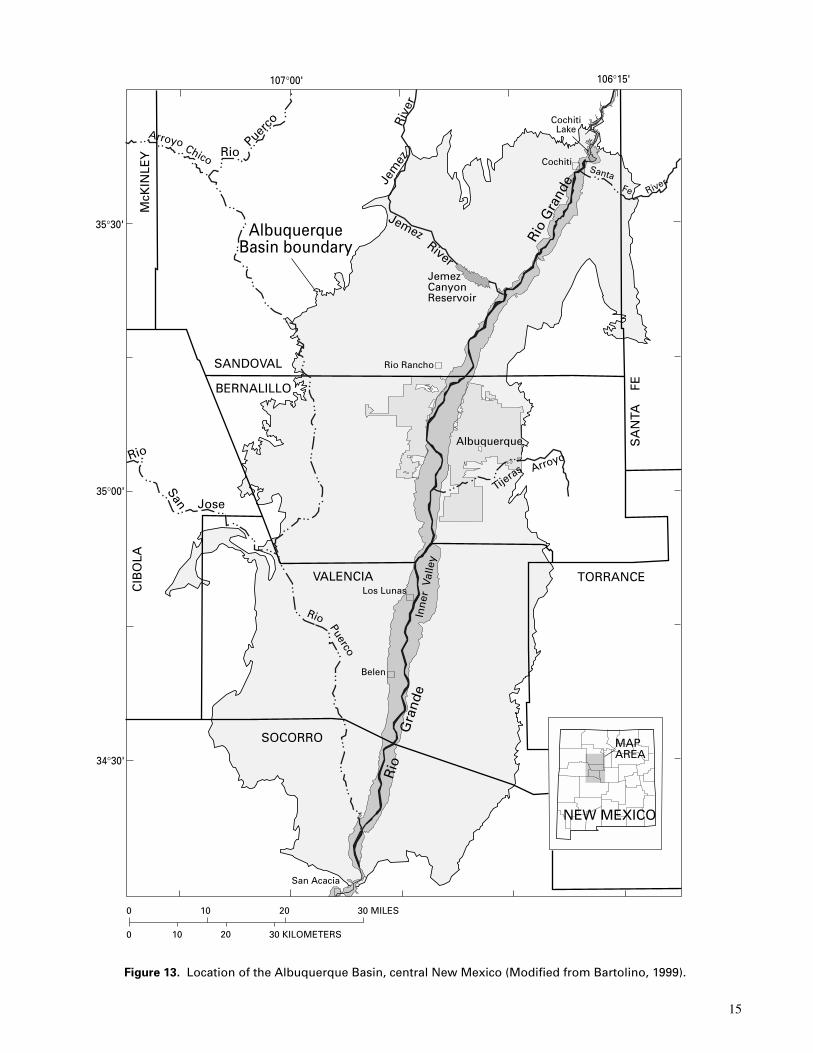
15

Figure 13. Location of the Albuquerque Basin, central New Mexico (Modified from Bartolino, 1999).

NEW MEXICO

MAPAREA

Chico RioPuer

co

AlbuquerqueBasin boundary

Jem

ezR

iver

JemezRiver

Rio

San Jose

San Acacia

Tijeras Arroyo

Albuquerque

Inne

r V

alle

y

Los Lunas

Belen

Rio Rancho

Cochiti

JemezCanyonReservoir

SantaFe River

CochitiLake

SANDOVAL

BERNALILLO

VALENCIA

Rio

Puerco

McK

INLE

Y

TORRANCE

SOCORRO

SA

NTA

F

E

10 20 30 MILES

0

0

10 20 30 KILOMETERS

107°00' 106°15'

35°00'

34°30'

35°30'

CIB

OLA

Rio

Gra

nde

Rio

Gra

nde

Arroyo

16

ground-water flow system, but the location and amounts ofthe sources and sinks of water to the system (that is, theboundary conditions) ultimately constrain the amount ofwater available for use. Therefore, accurate definition of theboundary conditions is very important to the accurate simula-tion of the basin. Kernodle and others (1995) used 11 layersand a finite difference grid of 244 rows and 178 columns torepresent the Santa Fe Group aquifer with the computer codeMODFLOW. The grid spacing varies from 656 feet (200meters) on a side in the Albuquerque area to a maximum of3,280 feet (1 kilometer) on a side at the basin margins. Theinvestigators described in detail the physical boundaries ofthe basin and their representation of them in the model.

Major hydrologic boundaries caused by physical fea-tures of the ground-water flow system of the AlbuquerqueBasin are: (1) mountain front and tributary recharge, (2)ground-water inflow from adjacent basins, (3) irrigationseepage, (4) septic-field return flow, (5) river, canal, and res-ervoir leakage, (6) drain seepage, and (7) riparian and wet-land evapotranspiration. The specific representation of thehydrologic boundaries as model boundary conditions is asfollows.

Boundary conditions associated with physical features atthe lateral extent of the model

The mountain front and tributary recharge was treated inthe model as a specified flow boundary in the upper mostlayer of the model. The flow rates specified along the bound-ary and along the few major mountain front streams areshown in figure 15. This represents a major source of inflowto the ground-water system under predevelopment condi-tions. The ground-water inflow from adjacent basins wasalso treated as a specified flow condition, and these valuesare also shown on figure 15. However, the flow from adja-cent basins was placed in model layers 5 through 9, ratherthan in the uppermost layer.

Boundary conditions associated with physical features atthe bottom of the model

The bottom of the model was represented as a no-flowcondition. There is no specific lithologic change at the bot-tom of the model, but rather the deposits decrease in perme-ability with depth. The vertical location of the boundary wasselected such that the materials below the bottom of themodel were thought to be of very low permeability and itwas below the producing zones of any production wells.

Boundary conditions associated with physical features atthe top of the model

The top of the model was represented as an unconfinedaquifer. The water-table elevation (and therefore the satu-rated thickness) changes as part of the model solution. No ar-eal recharge due directly to precipitation was simulated onthe top boundary.

For seepage from excess irrigation water, it was assumedthat approximately one third of the water applied to fieldsseeps through the soil profile and becomes recharge. Aftercalculation, it was determined that this amount of recharge is

one foot annually over the area being irrigated. Thus, a speci-fied flow of one foot per year was simulated over the area ofknown irrigation. This area changed size and shape over theperiod of simulation and the area of the specified flowchanged accordingly. The return flow from septic-field dis-posal was also treated as a specified flow. The populationwithin each model cell, in areas not served by sewer systems,was assumed to discharge, to the uppermost active layer, 75gallons per day per person, which is 75 percent of estimatedrural per capita domestic use. The amount of flow changedover time on the basis of estimates of changes in population.

River, canal, and reservoir interaction is a key aspect ofthe Albuquerque Basin ground-water system. The MOD-FLOW ‘River’ package is used to treat these features as non-linear, head-dependent flow boundaries (fig. 3E). The loca-tions of the river, canals, and reservoirs changed throughtime after 1935, and these changes were simulated in themodel. For the simulation period of 1901 through 1935 therewere no canals and reservoirs, and only the Rio Grande wassimulated.

A basin-wide network of drains was constructed in theAlbuquerque Basin in the early 1930’s. Riverside drains wereconstructed to intercept leakage from the Rio Grande thatflowed toward areas in the valley that were at altitudes lowerthan the streambed. The ‘Drain’ package in MODFLOW wasused to simulate these important hydrologic features as non-linear, head dependent boundaries. Under this representation,the drain only gains seepage, and the rate is proportional tothe altitude of the head in the aquifer above the drain eleva-tion (fig. 3D). The drains, rivers, and canals can all exist inthe same model cell, and although the local flow rates are notnecessarily accurate, it is assumed that they produce the ap-propriate flows on a regional scale.

Riparian and wetland evapotranspiration was conceptu-alized as the major discharge boundary for the system undernatural conditions. As discussed in the previous section,however, this component of a ground-water system is verydifficult to measure and approximate mathematically. Land-use-cover data were used to approximate the extent of thearea that would be undergoing evapotranspiration over time.The MODFLOW ‘Evapotranspiration’ package was used tosimulate the process, with a maximum rate of 2.6 feet peryear for heads at land surface, decreasing linearly to a rate ofzero for heads at a depth of 20 feet or more below land sur-face. Because this major outflow from the ground-water sys-tem cannot be measured directly, it has to be checked for rea-sonableness against measured surface-water flows and othermeasurable components of the ground-water system.

Water budget for the system

The simulated water budgets for predevelopment and for1994, as presented by Kernodle and others (1995), are listedin table 3. The importance of the boundary conditions isreadily observed in that all of the components in the table,except for water from storage and ground-water withdrawals,are from boundary flows. Only if the conceptualization andmathematical representations are appropriate does the simu-

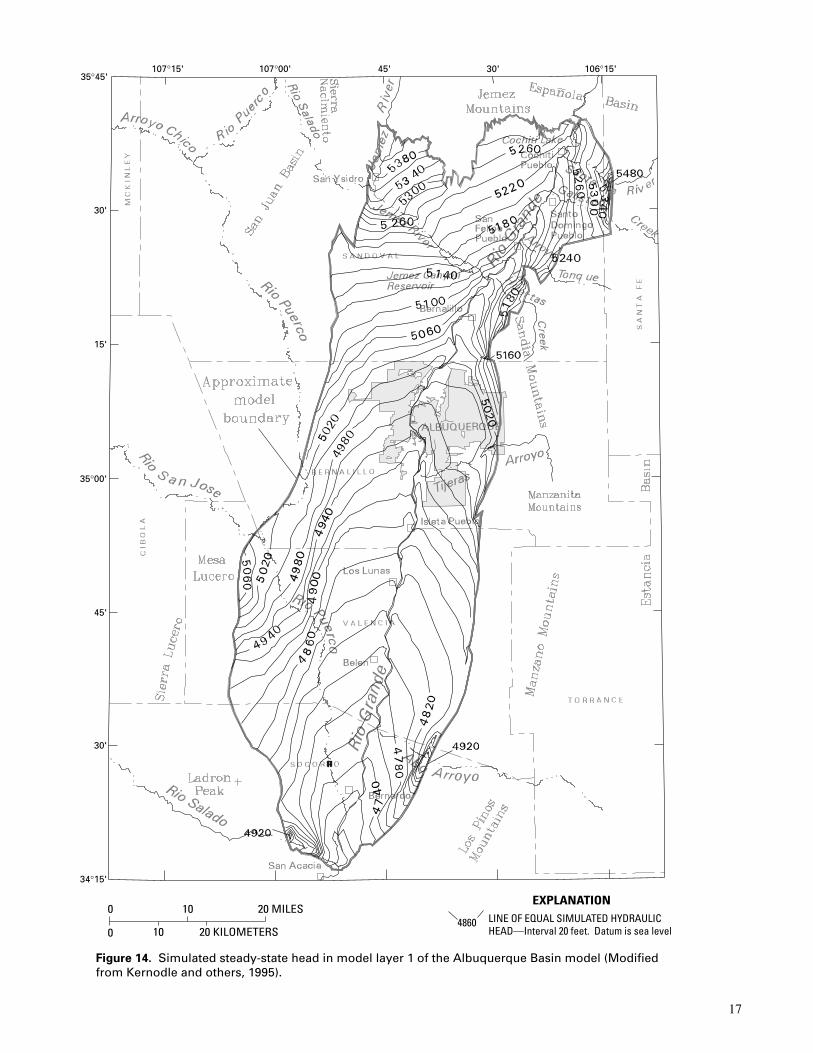
17

Figure 14. Simulated steady-state head in model layer 1 of the Albuquerque Basin model (Modifiedfrom Kernodle and others, 1995).

LINE OF EQUAL SIMULATED HYDRAULIC HEAD—Interval 20 feet. Datum is sea level

4860 0

0

10

10 20 KILOMETERS

20 MILESEXPLANATION

107°15'35°45'

30'

15'

35°00'

45'

30'

34°15'

107°00' 106°15'45' 30'

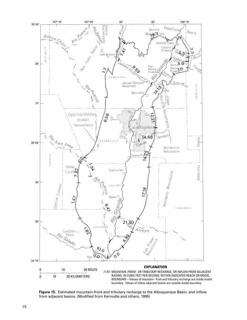
18

MOUNTAIN–FRONT OR TRIBUTARY RECHARGE, OR INFLOW FROM ADJACENT BASINS, IN CUBIC FEET PER SECOND, WITHIN INDICATED REACH OR MODEL BOUNDARY—Values of mountain– front and tributary recharge are inside model boundary. Values of inflow adjacent basins are outside model boundary

/1.47/ EXPLANATION

0

0

10

10 20 KILOMETERS

20 MILES

107°15'35°45'

30'

15'

35°00'

45'

30'

34°15'

107°00' 106°15'45' 30'

Figure 15. Estimated mountain-front and tributary recharge to the Albuquerque Basin, and inflowfrom adjacent basins. (Modified from Kernodle and others, 1995)

19

lation have any chance of accurately representing the actualsystem.

Conceptualization of the Long Island, New YorkGround-Water Flow System

Long Island is bounded on the north by Long IslandSound, on the east and south by the Atlantic Ocean, and onthe west by New York Bay and the East River (fig. 16).Long Island is divided into four counties—Kings, Queens,Nassau, and Suffolk. The source of water supply for the twowestern counties, Kings and Queens, which are part of NewYork City, is primarily surface water reservoirs locatednorth of the city. Ground water, however, is the only sourceof fresh water for the population of Nassau and SuffolkCounties, which is greater than 2.5 million people.

The ground-water system of Long Island consists of alayered sequence of aquifers and confining units, which dipgently to the south and east (fig. 17). The system is under-lain by crystalline bedrock that is virtually impermeable.Overlying the bedrock are hydrogeologic units of Creta-ceous age, which are in ascending order: the Lloyd aquifer,the Raritan confining unit, and the Magothy aquifer. Abovethese are deposits of Pleistocene age. The Gardiners Clay,an interglacial marine clay that separates the Magothy andthe overlying glacial aquifer, is present along the southshore of Long Island and has an irregular extent. Glacial de-posits consisting primarily of moraine and outwash overlieall of these units throughout the island. Several otherhydrogeologic units of local extent are also present.

Precipitation that infiltrates and percolates to the watertable is Long Island’s only natural source of freshwater be-cause the ground-water system is bounded on the bottom byrelatively impermeable bedrock and on the sides by salineground water or saline bays and the Atlantic Ocean. Aboutone-half the precipitation becomes recharge to the ground-water system; the rest flows as surface runoff to streams or islost through evapotranspiration. Most of the precipitationthat reaches the uppermost unconfined aquifer moves later-ally and discharges to streams and surrounding saltwaterbodies; the remainder seeps downward to recharge the deeperaquifers. Water enters these deeper aquifers very slowly inareas where confining units are present, but enters freelywhere the confining units are absent. Water in the deeperaquifers also moves seaward and eventually seeps into over-lying aquifers.

Long Island’s ground water has been developed over thepast three centuries. The present phase of ground-water de-velopment on the island began in the early 1950’s with theintroduction of large-scale sewer systems in the most heavilypopulated areas. The purpose of the sewers was to preventdomestic wastewater from entering the aquifer system, be-cause contaminants from this source were being detected indeep public-supply wells. Even though the sewers protect theaquifers from further contamination, they also prevent the re-plenishment (recharge) that the wastewater had provided tothe ground-water reservoir through the domestic wastewater-disposal systems. The wastewater is now diverted to sewage-

Predevelopment 1994

Mechanism Inflow OutflowNet (inflow

minusoutflow)

Net (inflowminus

outflow)Inflow

Mountain-front and tributary recharge 99,100 0 99,100 131,000

Ground-water inflow from adjacent basins 28,400 0 28,400

133,000

28,400

River, canal, and reservoir leakage 141,000 8,170 247,000

Drain seepage 0 0 0

Riparian and wetland evapotranspiration 0 261,000 -261,000

Irrigation seepage 0 0 0

0

0

0

28,300

Ground-water withdrawal 0 0 0

Septic-field return flow 0 0 0 8,220

Aquifer Storage 0 0 0 109,000

Total 268,000 269,000 -500 552,000

0

0

44,400

219,000

0

89,200

171,000

0

27,800

551,000

131,000

28,400

203,000

-219,000

-89,200

-171,000

28,300

8,220

81,200

920

Percent discrepancy 0.2 0.2

Outflow

Table 3. Simulated annual water budgets for the Albuquerque Basin for predevelopment and 1994 (Modified fromKernodle and others, 1995). [All values are in acre-feet per year]

20

treatment plants, whose effluent is discharged to the bays andoceans. The decrease in recharge has caused the water tablein the sewered areas to be substantially lowered, the baseflow of streams to be reduced or eliminated, and the lengthof perennial streams to be decreased. To aid in the manage-ment of this very important resource, several ground-water

flow models have been developed (Getzen, 1977; Reilly andHarbaugh, 1980; and Buxton and Smolensky, 1999).

The latest ground-water flow model of Long Island(Buxton and Smolensky, 1999) is a three-dimensional finite-difference model that uses the MODFLOW computer pro-gram developed by McDonald and Harbaugh (1988). The

NEW YORK

NEWJERSEY

CONNECTICUT

SUFFORKCOUNTY

QUEENSCOUNTY

Fire Island

New York Bay

KINGSCOUNTY

NASSAUCOUNTY

Manhattan

StatenIsland

LONG ISLAND

LONG ISLAND SOUND

74° 73° 72°

ATLANTICOCEAN

45°

0

0 10 20 KILOMETERS

10 20 MILES

LOCATIONMAP

East R

.

Figure 16. Location of Long Island, New York. (From Buxton and Smolensky, 1999)

0 1 2 3 4 MILES

0 1 2 3 4 KILOMETERS

AREA OF SALTY GROUND-WATER

LINE OF EQUAL HYDRAULIC HEAD–Contourinterval is 20 feet. Datum is sea level

STREAMLINE (LINE OF EQUAL STREAM-FUNCTION VALUE)–Contour interval variable. Arrow indicates direction of flow

SALTWATER INTERFACE

20

.62

EXPLANATION

250

-250

-500

-750

-1,000

-1,250

-1,500

-1,750

-2,000

-2,250

SEALEVEL

FEETNORTH SOUTH

A A'

Long Island Sound Atlantic Ocean

UPPER GLACIAL AQUIFER

MAGOTHY

AQUIFER

RARITAN CONFINING UNIT

GARDINERS CLAY

LLOYD AQUIFER

Water table

BEDROCK

20 40

60

80

20

40

6080

.40

.45

.60

.62

.65

.75.85

.80

.70

.63

.50

.55

Figure 17. Hydrogeologic section of Long Island, New York. (From Buxton and Smolensky, 1999)

21

finite-difference grid has 46 rows and 118 columns (fig. 18),and each block is 4,000 by 4,000 feet. The model representsthe aquifer units with 4 layers (fig. 19). The hydrologic fea-tures that form the boundaries of the Long Island ground-water system and their representation in the model are asfollows.

Boundary Conditions Associated with Physical Features atthe Lateral Extent of the Model

Salt surface-water bodies at the surface and salt-waterinterfaces at depth bound the lateral extent of the Long Is-land fresh ground-water system. The salt surface-water bod-ies (Long Island Sound, the Atlantic Ocean, Great SouthBay, and others) are treated as a specified head in the toplayer of the model. The saltwater interface is treated as a no-flow boundary in the deeper aquifers and model layers. Inareas where the deeper aquifers are overlain by a confiningunit and extend below a body of overlying salty ground wa-

ter, subsea discharge can occur through the confining unitinto the overlying aquifer that contains salty ground water.This subsea discharge boundary is represented as a specifiedhead at the top of the confining unit, with the head at the topof the confining unit representing an equivalent freshwaterhead calculated to take into account the density differencebetween the overlying salty ground water and the dischargingfresh ground water [see Buxton and Smolensky (1999) for anexplanation of this specific boundary or Reilly (1993) for ageneral explanation of equivalent freshwater head].

Boundary Conditions Associated with Physical Features atthe Bottom of the Model

The Long Island fresh ground-water system is boundedbelow by relatively impermeable Precambrian bedrock.Thus, the bottom boundary of the model representing thecontact of the permeable deposits with the bedrock is simu-lated as a no-flow boundary.

10 20 30 40 50 60 70 80 90 100 110

10

00

20

30

40

COLUMNS

RO

WS

B. MODEL GRID

A

A

0 5 10 15 20 MILES

0 5 10 15 20 KILOMETERS

74°00' 41°00' 73°00'

40°45'

40°30'

A. STREAMS AND SHORE

Edge ofmodeledarea

Kings

QueensNassau Suffolk

Figure 18. Areal representation of Long Island, New York, by the regional ground-water flow model: (A) Actualmap view; and (B) Discretized map view. (Modified from Buxton and Smolensky, 1999)

22

Boundary Conditions Associated with Physical Features atthe Top of the Model

The top of Long Island’s ground-water system is thewater table that bounds the saturated ground-water system.The model represents the water table as a free surface thatmoves in response to stress. Areal recharge due to precipi-tation is simulated as a specified flow at the uppermost ac-tive cells.

Streams are represented in the model in two differentways, depending on whether the simulation is a steady-state simulation of known conditions or a transient simula-tion in which variations in ground-water discharge to thestreams is to be determined. Streams are represented asspecified discharge boundaries for steady-state simulations

of known historical conditions, and as nonlinear, head-dependent strictly gaining boundaries (as a drain inMODFLOW) for simulations in which changes in base floware simulated.

Water Budget for the SystemThe simulated water budgets for predevelopment and

for the period 1968 to 1983, as presented by Buxton andSmolensky (1999), are listed in table 4. The importance ofthe boundary conditions is readily observed in that all of thecomponents in the table, except for pumpage, are fromboundary flows. Only if the conceptualization and math-ematical representations of the boundaries are appropriatedoes the simulation have any chance of accurately represent-ing the actual system.

Bedrock

Water tableLong IslandSound Atlantic Ocean

200

-200

-400

-600

-800

-1,000

-1,200

-1,400

Sealevel

FEET

200

-200

-400

-600

-800

-1,000

-1,200

-1,400

Sealevel

FEET

10 15 20 25 30 35

10 15 20 25 30 35

VERTICAL EXAGGERATION X25

VERTICAL EXAGGERATION X25

EXPLANATION

Upper glacial aquifer

Gardiners Clay

Jameco aquifer

Magothy aquifer

Raritan confining unit

Lloyd aquifer

NORTH SOUTH

MODEL ROW NUMBER, 4000 FEET PER ROW

A

B

Figure 19. Cross-sectional representation of the ground-water flow system, Long Island, New York, in the regionalground-water flow model: (A) Actual cross section; and (B) Discretized cross section. Section located near A-A’ infigure 18 (From Buxton and others, 1999)

23

SUMMARY AND CONCLUSIONSWhen described mathematically, ground-water flow

problems are classified as boundary value problems. This in-dicates that the selection of appropriate boundary conditionsis critical to the accurate definition and analysis of the prob-lem. In ground-water models, which are used for analyzingground-water flow problems, the specification of the bound-ary conditions usually defines the source of water to the sys-tem and its ultimate manner of discharge. Thus, boundaryconditions are one of the key aspects in the properconceptualization of a ground-water system and representa-tion of that system in a numerical computer model.

Conceptualizing the physical processes at the boundariesof a ground-water system and devising a mathematical coun-terpart that can be incorporated into a model is usually notstraightforward. Appendix 1 lists many of the “Packages”that can be used in the U.S. Geological Survey ModularThree-Dimensional Ground-Water Flow Model(MODFLOW) to represent physical features of a ground-wa-ter system as mathematical boundary conditions. From thislist, it is apparent that many different “Packages” can be usedto simulate the same physical feature in a ground-water sys-tem. Depending upon the conceptualization and the expecteduse of the model, different mathematical representations canbe used for the same feature.

The mathematical boundary conditions that representphysical features of the ground-water system being modeledare based on certain assumptions regarding the use of themodel, the amount of stress that will be simulated, and theaccuracy required. If the model is used to evaluate conditionsthat are no longer the same as the design assumptions, thesimulation results will be invalid. The analyst must carefullyevaluate the source of water to the ground-water system, thelimits on the quantities of water available from the source,and potential changes to the system, and then select the ap-propriate mathematical counterpart. In addition, during the

use of a model the analyst must continually check the simu-lation results to ensure that basic assumptions that weremade regarding the boundary conditions during their selec-tion are not violated.

Ground-water models are useful tools in analyzingground-water flow problems. The proper design of a model,however, depends on a clear conceptualization of the flowsystem in nature and an understanding of the strengths andweaknesses of the various mathematical options available tosimulate the various aspects of the actual system. A few ofthese mathematical representations of specific boundary con-ditions were discussed in this report to highlight the level ofinvolvement that the analyst should have in the proper designand execution of ground-water models.

ACKNOWLEDGMENTSThe technical review and improvement of the report by

Paul Barlow, William Cunningham, O. Lehn Franke, ArlenHarbaugh, and Douglas McAda is gratefully acknowledged.Chet Zenone provided editorial review and assistance, andPatricia Greene prepared the final report and illustrations.

SELECTED REFERENCESAnderson, M.P., and Woessner, W.W., 1992, Applied ground-

water modeling: Academic Press, Inc., San Diego, CA,381 p.

Bartolino, J.R., 1999, U.S. Geological Survey Middle RioGrande Basin Study – Proceedings of the Third AnnualWorkshop, Albuquerque, New Mexico, February 24-25,1999: U.S. Geological Survey Open-File Report 99-203,95 p.

Buxton, H.T., and Smolensky, D.A., 1999, Simulation of theeffects of development of the ground-water flow systemof Long Island, New York: U.S. Geological Survey Water-Resources Investigations Report 98-4069, 57 p.

Buxton, H.T., Smolensky, D.A., and Shernoff, P.K., 1999,

Predevelopment 1968–1983

Mechanism Inflow OutflowNet (inflow

minusoutflow)

Net (inflowminus

outflow)Inflow

Recharge from precipitation and returned water

Pumpage

Stream discharge

Discharge at the shore

Deep subsea discharge

Total

1,126

0

0

0

1,126

0

0

407

325

503

1,293

58

1,293

0

0

0

1,293

0

1,126

0

-460

-585

0

-81

1,293

-407

-325

-503

0

-58

0

0

460

585

1,126

81

Outflow

Table 4. Simulated annual water budgets for the Long Island, New York ground-water system for predevelopment andthe period of 1968-1983 (Modified from Buxton and Smolensky, 1999). [All values are in million gallons per day]

24

Feasibility of using ground water as a supplemental sup-ply for Brooklyn and Queens, New York: U.S. GeologicalSurvey Water-Resources Investigations Report 98-4070,33 p.

Cheng, X., and Anderson, M.P., 1993, Numerical simulationof ground-water interaction with lakes allowing for fluctu-ating lake levels: Ground Water, v. 31, no. 6, p. 929-933.

Collins, R.E., 1961, Flow of fluids through porous materials:Reinhold Publishing Corp., N.Y., 270 p.

Eberts, S.M., and George, L.L., 2000, Regional ground-waterflow and geochemistry in the Midwestern Basins andArches Aquifer System in parts of Indiana, Ohio, Michi-gan, and Illinois: U.S. Geological Survey Professional Pa-per 1423-C, 103 p.

Essaid, H.I., 1990, SHARP—A quasi-three-dimensional fi-nite-difference simulation model for freshwater and salt-water flow in layered coastal aquifer systems: U.S. Geo-logical Survey Water-Resources Investigations Report 90-4130, 181 p.

Fenske, J.P., Leake, S.A., and Prudic, D.E., 1996, Documen-tation of a computer program (RES1) to simulate leakagefrom reservoirs using the modular finite-differenceground-water flow model (MODFLOW): U.S. GeologicalSurvey Open-File Report 96-364, 51 p.

Franke, O.L., Reilly, T.E., and Bennett, G.D., 1987, Defini-tion of boundary and initial conditions in the analysis ofsaturated ground-water flow systems – An introduction:Techniques of Water-Resources Investigations of theUnited States Geological Survey, Book 3, Chapter B5,15 p.

Getzen, R.T., 1977, Analog-model analysis of regional three-dimensional flow in the ground-water reservoir of LongIsland, New York: U.S. Geological Survey ProfessionalPaper 982, 49 p.

Grannemann, N.G., Hunt, R.J., Nicholas, J.R., Reilly, T.E.,and Winter, T.C., 2000, The importance of ground waterto the Great Lakes Region: U.S. Geological Survey Water-Resources Investigations Report 00-4008, 12 p.

Jobson, H.E., and Harbaugh, A.W., 1999, Modifications tothe diffusion analogy surface-water flow model(DAFLOW) for coupling to the modular finite-differenceground-water flow model (MODFLOW): U.S. GeologicalSurvey Open-File Report 99-217, 107 p.

Kernodle, J.M., McAda, D.P., and Thorn, C.R., 1995, Simu-lation of ground-water flow in the Albuquerque Basin,central New Mexico, 1901-1994, with projections to2020: U.S. Geological Survey Water-Resources Investiga-tions Report 94-4251, 114 p.

Konikow, L.F., and Bredehoeft, J.D., 1992, Ground-watermodels cannot be validated: Advances in Water Re-sources, v. 15, p. 75-83.

Koreny, J.S., Mitsch, W.J., Bair, E.S., and Wu, X., 1999, Re-gional and local hydrology of a created riparian wetlandsystem: Wetlands, v. 19, no. 1, p. 182-193.

Leake, S.A., and Lilly, M.R., 1997, Documentation of a com-puter program (FHB1) for assignment of transient speci-fied-flow and specified-head boundaries in applications of

the Modular Finite-Difference Ground-Water Flow Model(MODFLOW): U.S. Geological Survey Open-File Report97-571, 50 p.

Masterson, J.P., and Barlow, P.M., 1997, Effects of simulatedground-water pumping and recharge on ground-waterflow in Cape Cod, Martha’s Vineyard, and Nantucket Is-land Basins, Massachusetts: U.S. Geological Survey Wa-ter-Supply Paper 2447, 79 p.

McDonald, M.G., and Harbaugh, A.W., 1988, A modularthree-dimensional finite-difference ground-water flowmodel: Techniques of Water-Resources Investigations ofthe United States Geological Survey, Book 6, Chapter A1,586 p.

McDonald, M.G., Harbaugh, A.W., Orr, B.R., and Ackerman,D.J., 1992, A method of converting no-flow cells to vari-able-head cells for the U.S. Geological Survey modular fi-nite- difference ground-water flow model: U.S. Geologi-cal Survey Open-File Report 91-536, 99 p.

Merritt, M.L., and Konikow, L.F., 2000, Documentation of acomputer program to simulate lake-aquifer interaction us-ing the MODFLOW ground-water flow model and theMOC3D solute-transport model: U.S. Geological SurveyWater-Resources Investigations Report 00-4167, 146 p.

Prudic, D.E., 1989, Documentation of a computer program tosimulate stream-aquifer relations using a modular, finite-difference, ground-water flow model: U.S. GeologicalSurvey Open-File Report 88-729, 113 p.

Reilly, T.E., 1990, Simulation of dispersion in layered coastalaquifer systems: Journal of Hydrology, v. 114, p. 211-228

Reilly, T.E., 1993, Analysis of ground-water systems infreshwater-saltwater environments: in Regional ground-water quality (William Alley, editor): Van NostrandReinhold, New York, NY, p. 443-469.

Reilly, T.E., Franke, O.L., and Bennett, G.D., 1987, The prin-ciple of superposition and its application in ground-waterhydraulics: Techniques of Water-Resources Investigationsof the United States Geological Survey, Book 3, ChapterB6, 28 p.

Reilly, T.E., and Goodman, A.S., 1985, Quantitative analysisof saltwater-freshwater relationships in groundwater sys-tems—A historical perspective: Journal of Hydrology, v.80, no. 1-2, p. 125-160.

Reilly, T.E., and Harbaugh, A.W., 1980, A comparison ofanalog and digital modeling techniques for simulatingthree-dimensional ground-water flow on Long Island:U.S. Geological Survey Water-Resources Investigations80-14, 40 p.

Swain, E.D., Howie, Barbara, and Dixon, Joann, 1996, De-scription and field analysis of a coupled ground-water/sur-face-water flow model (MODFLOW/BRANCH) withmodifications for structures and wetlands in southernDade County, Florida: U.S. Geological Survey Water-Re-sources Investigations Report 96-4118, 67 p.

Swain, E.D., and Wexler, E.J., 1993, A coupled surface-waterand ground-water flow model for simulation of stream-aquifer interaction: U.S. Geological Survey Open-FileReport 92-138, 162 p.

25

Thorn, C.R., McAda, D.P., and Kernodle, J.M., 1993, Geo-hydrologic framework and hydrologic conditions in theAlbuquerque Basin, central New Mexico: U.S. GeologicalSurvey Water-Resources Investigations Report 93-4149,106 p.

Wilkins, D.W., 1998, Summary of the Southwestern AlluvialBasins Regional Aquifer-System analysis in parts of Colo-rado, New Mexico, and Texas: U.S. Geological SurveyProfessional Paper 1407-A, 49 p.

Wilson, W.E., and Moore, J.E., 1998, Glossary of hydrology:American Geological Institute, Alexandria, VA, 248 p.

Winston, R.B., 1996, Design of an urban, ground-water-dominated wetland: Wetlands, v. 16, no. 4, p. 524-531.

Winter, T.C., Harvey, J.W., Franke, O.L., and Alley, W.M.,1998, Ground water and surface water – A single re-source: U.S. Geological Survey Circular 1139, 79 p.

26

MODFLOW-PACKAGENAME

PHYSICAL FEATURES THATCAN BE SIMULATED

BOUNDARY-CONDITION TYPE

REFERENCE

Basic Package (BAS) Stream, lake, ocean, wetland,interbasin flow, springs

Specified Head McDonald andHarbaugh(1988)

Well Package (WEL) Well, stream, interbasin flow,earth materials of low hydraulicconductivity

Specified Flow McDonald andHarbaugh(1988)

Recharge Package (RCH) Areal recharge or discharge Specified Flow McDonald andHarbaugh(1988)

General-Head BoundaryPackage (GHB)

Stream, lake, ocean, wetland,interbasin flow

Head-DependentFlow

McDonald andHarbaugh(1988)

River Package (RIV) Stream, lake, wetland Nonlinear Head-Dependent Flow


Drain Package (DRN) Stream, lake, drain, wetland,springs

Nonlinear Head-Dependent Flow


EvapotranspirationPackage (EVT)

Evapotranspiration Nonlinear Head-Dependent Flow


Block Centered FlowPackage (BCF1)

Water table Free-Surface McDonald andHarbaugh(1988)

Stream Package (STR) Stream, drain Nonlinear Head-Dependent Flow

Prudic (1989)

Block Centered FlowPackage 2 (BCF2)

Water table with rewetting Free-Surface McDonald andothers (1992)

BRANCH Surface-WaterModel Package (BRC)

Stream Nonlinear Head-Dependent Flow

Swain andWexler (1993)

Reservoir Package (RES) Reservoir, lake, wetland Nonlinear Head-Dependent Flow

Fenske andothers (1996)

Flow and Head boundaryPackage (FHB)

Stream, lake, ocean, wetland,interbasin flow

Transient SpecifiedFlow and Head

Leake and Lilly(1997)

Diffusion AnalogySurface-Water FlowPackage (DAF)

Stream Nonlinear Head-Dependent Flow

Jobson andHarbaugh(1999)

Lake Package (LAK3) Lake, wetland Nonlinear Head-Dependent Flow

Merritt andKonikow (2000)

Appendix 1. List of “Packages” in the U.S. Geological Survey Modular Three-Dimensional Ground-Water Flow Model(MODFLOW) used to represent physical features of a ground-water system as mathematical boundary conditions

27

TECHNIQUES OF WATER-RESOURCESINVESTIGATIONS OF THE U.S. GEOLOGICAL SURVEYThe U.S.G.S. publishes a series of manuals describing proceduresfor planning and conducting specialized work in water-resourcesinvestigations. The material is grouped under major subjectheadings called books and is further divided into sections andchapters. For example, section A of book 3 (Applications ofHydraulics) pertains to surface water. The chapter, the unit ofpublication, is limited to a narrow field of subject matter. Thisformat permits flexibility in revision and publication as the needarises.The reports listed below are for sale by the U.S.G.S., InformationServices, Box 25286, Federal Center, Denver, Colorado 80225(authorized agent of the Superintendent of Documents, GovernmentPrinting Office). Prepayment is required. Remittance should bemade in the form of a check or money order payable to the “U.S.Geological Survey.” Prices are not included because they are subjectto change. Current prices can be obtained by writing to the aboveaddress. When ordering or inquiring about prices for any of thesepublications, please give the title, book number, chapter number,and mention the “U.S. Geological Survey Techniques of Water-Resources Investigations.”

Book 1. Collection of Water Data by Direct Measurement

Section D. Water Quality

1-D1. Water temperature-influential factors, field measurement,and data presentation, by H. H. Stevens, Jr., J.F. Ficke, andG. F. Smoot: USGS-TWRI book 1, chap. D1. 1975. 65pages.

1-D2. Guidelines for collection and field analysis of ground-watersamples for selected unstable constituents, by W.W. Wood:USGS-TWRI book 1, chap. D2. 1976. 24 pages.

Book 2. Collection of Environmental Data

Section D. Surface Geophysical Methods

2-D1. Application of surface geophysics to ground-waterinvestigations, by A.A. R. Zohdy, G.P. Eaton, and D.R.Mabey: USGS-TWRI book 2, chap. D1. 1974. 116 pages.

2-D2. Application of seismic-refraction techniques to hydrologicstudies, by F.P. Haeni: USGS-TWRI book 2, chap. D2. 1988.86 pages.

Section E. Subsurface Geophysical Methods

2-E1. Application of borehole geophysics to water-resourcesinvestigations, by W.S. Keys and L.M. MacCary: USGS-TWRI book 2, chap. E1. 1971. 126 pages.

2-E2. Borehole geophysics applied to ground-water investigations,by W.S. Keys: USGS-TWRI book 2, chap. E2. 1990. 150pages.

Section F. Drilling and Sampling Methods

2-F1. Application of drilling, coring, and sampling techniques totest holes and wells, by Eugene Shuter and W.E. Teasdale:USGS-TWRI book 2, chap. F1. 1989. 97 pages.

Book 3. Applications of Hydraulics

Section A. Surface-Water Techniques

3-A1. General field and office procedures for indirect dischargemeasurements, by M.A. Benson and Tate Dalrymple: USGS-TWRI book 3, chap. A1. 1967. 30 pages.

3-A2. Measurement of peak discharge by the slope-area method,by Tate Dalrymple and M.A. Benson: USGS-TWRI book 3,chap. A2. 1967. 12 pages.

3-A3. Measurement of peak discharge at culverts by indirectmethods, by G.L. Bodhaine: USGS-TWRI book 3, chap. A3.1968. 60 pages.

3-A4. Measurement of peak discharge at width contractions byindirect methods, by H.F. Matthai: USGS-TWRI book 3,chap. A4. 1967. 44 pages.

3-A5. Measurement of peak discharge at dams by indirect methods,by Harry Hulsing: USGS-TWRI book 3. chap. A5. 1967. 29pages.

3-A6. General procedure for gaging streams, by R.W. Carter andJacob Davidian: USGS-TWRI book 3, chap. A6. 1968. 13pages.

3-A7. Stage measurement at gaging stations, by T.J. Buchanan andW.P. Somers: USGS-TWRI book 3, chap. A7. 1968. 28pages.

3-A8. Discharge measurements at gaging stations, by T.J.Buchanan and W.P. Somers: USGS-TWRI book 3, chap. A8.1969. 65 pages.

3-A9. Measurement of time of travel in streams by dye tracing, byF.A. Kilpatrick and J.F. Wilson, Jr.: USGS-TWRI book 3,chap. A9. 1989. 27 pages.

3-Al0. Discharge ratings at gaging stations, by E.J. Kennedy:USGS-TWRI book 3, chap. A10. 1984. 59 pages.

3-A11. Measurement of discharge by the moving-boat method, byG.F. Smoot and C.E. Novak: USGS-TWRI book 3, chap.A11. 1969. 22 pages.

3-A12. Fluorometric procedures for dye tracing, Revised, by J.F.Wilson, Jr., E.D. Cobb, and F.A. Kilpatrick: USGS-TWRIbook 3, chap. A12. 1986. 34 pages.

3-A13. Computation of continuous records of streamflow, by E.J.Kennedy: USGS-TWRI book 3, chap. A13. 1983. 53 pages.

3-A14. Use of flumes in measuring discharge, by F.A. Kilpatrickand V.R. Schneider: USGS-TWRI book 3, chap. A14. 1983.46 pages.

3-A15. Computation of water-surface profiles in open channels, byJacob Davidian: USGS-TWRI book 3, chap. A15. 1984. 48pages.

3-A16. Measurement of discharge using tracers, by F.A. Kilpatrickand E.D. Cobb: USGS-TWRI book 3, chap. A16. 1985. 52pages.

3-A17. Acoustic velocity meter systems, by Antonius Laenen:USGS-TWRI book 3, chap. A17. 1985. 38 pages.

3-A18. Determination of stream reaeration coefficients by use oftracers, by F.A. Kilpatrick, R.E. Rathbun, NobuhiroYotsukura, G.W. Parker, and L.L. DeLong: USGS-TWRIbook 3, chap. A18. 1989. 52 pages.

3-A19. Levels at streamflow gaging stations, by E.J. Kennedy:USGS-TWRI book 3, chap. A19. 1990. 31 pages.

3-A20. Simulation of soluble waste transport and buildup insurface waters using tracers, by F.A. Kilpatrick: USGS-TWRI book 3, chap. A20. 1993. 38 pages.

3-A21 Stream-gaging cableways, by C. Russell Wagner: USGS-TWRI book 3, chap. A21. 1995. 56 pages.

Section B. Ground-Water Techniques

3-B1. Aquifer-test design, observation, and data analysis, by R.W.Stallman: USGS-TWRI book 3, chap. B1. 1971. 26 pages.

3-B2. ntroduction to ground-water hydraulics, a programed text forself-instruction, by G.D. Bennett: USGS-TWRI book 3,chap. B2. 1976. 172 pages.

3-B3. Type curves for selected problems of flow to wells inconfined aquifers, by J.E. Reed: USGS-TWRI book 3, chap.B3. 1980. 106 pages.

3-B4. Regression modeling of ground-water flow, by R.L. Cooleyand R.L. Naff: USGS-TWRI book 3, chap. B4. 1990. 232pages.

28

3-B4. Supplement 1. Regression modeling of ground-water flow —Modifications to the computer code for nonlinear regressionsolution of steady-state ground-water flow problems, byR.L. Cooley: USGS-TWRI book 3, chap. B4. 1993. 8 pages.

3-B5. Definition of boundary and initial conditions in the analysisof saturated ground-water flow systems-An introduction, byO.L. Franke, T.E. Reilly, and G.D. Bennett: USGS-TWRIbook 3, chap. B5. 1987. 15 pages.

3-B6. The principle of superposition and its application in ground-water hydraulics, by T.E. Reilly, O.L. Franke, and G.D.Bennett: USGS-TWRI book 3, chap. B6. 1987. 28 pages.

3-B7. Analytical solutions for one-, two-, and three-dimensionalsolute transport in ground-water systems with uniform flow,by E.J. Wexler: USGS-TWRI book 3, chap. B7. 1992. 190pages.

3-B8. System and boundary conceptualization in ground-water flowsimulation, by T.E. Reilly: USGS-TWRI book 3, chap. B8.2001. 29 pages.

Section C. Sedimentation and Erosion Techniques

3-C1. Fluvial sediment concepts, by H.P. Guy: USGS-TWRI book3, chap. C1. 1970. 55 pages.

3-C2. Field methods for measurement of fluvial sediment, by T.K.Edwards and G.D. Glysson: USGS-TWRI book 3, chap. C2.1999. 89 pages.

3-C3. Computation of fluvial-sediment discharge, by GeorgePorterfield: USGS-TWRI book 3, chap. C3. 1972. 66 pages.

Book 4. Hydrologic Analysis and Interpretation

Section A. Statistical Analysis

4-A1. Some statistical tools in hydrology, by H.C. Riggs: USGS-TWRI book 4, chap. A1. 1968. 39 pages.

4-A2. Frequency curves, by H.C. Riggs: USGS-TWRI book 4,chap. A2. 1968. 15 pages.

Section B. Surface Water

4-B1. Low-flow investigations, by H.C. Riggs: USGS-TWRI book4, chap. B1. 1972. 18 pages.

4-B2. Storage analyses for water supply, by H.C. Riggs and C.H.Hardison: USGS-TWRI book 4, chap. B2. 1973. 20 pages.

4-B3. Regional analyses of streamflow characteristics, by H.C.Riggs: USGS-TWRI book 4, chap. B3. 1973. 15 pages.

Section D. Interrelated Phases of the Hydrologic Cycle

4-D1. Computation of rate and volume of stream depletion bywells, by C.T. Jenkins: USGS-TWRI book 4, chap. D1.1970. 17 pages.

Book 5. Laboratory Analysis

Section A. Water Analysis

5-A1. Methods for determination of inorganic substances in waterand fluvial sediments, by M.J. Fishman and L.C. Friedman,editors: USGS-TWRI book 5, chap. A1. 1989. 545 pages.

5-A2. Determination of minor elements in water by emissionspectroscopy, by P.R. Barnett and E.C. Mallory, Jr.: USGS-TWRI book 5, chap. A2. 1971. 31 pages.

5-A3. Methods for the determination of organic substances in waterand fluvial sediments, edited by R.L. Wershaw, M.J.Fishman, R.R. Grabbe, and L.E. Lowe: USGS-TWRI book5, chap. A3. 1987. 80 pages.

5-A4. Methods for collection and analysis of aquatic biological andmicrobiological samples, by L.J. Britton and P.E. Greeson,editors: USGS-TWRI book 5, chap. A4. 1989. 363 pages.

5-A5. Methods for determination of radioactive substances in waterand fluvial sediments, by L.L. Thatcher, V.J. Janzer, andK.W. Edwards: USGS-TWRI book 5, chap. A5. 1977. 95pages.

5-A6. Quality assurance practices for the chemical and biologicalanalyses of water and fluvial sediments, by L.C. Friedmanand D.E. Erdmann: USGS-TWRI book 5, chap. A6. 1982.181 pages.

Section C. Sediment Analysis

5-C1. Laboratory theory and methods for sediment analysis, byH.P. Guy: USGS-TWRI book 5, chap. C1. 1969. 58 pages.

Book 6. Modeling Techniques

Section A. Ground Water

6-A1. A modular three-dimensional finite-difference ground-waterflow model, by M.G. McDonald and A.W. Harbaugh:USGS-TWRI book 6, chap. A1. 1988. 586 pages.

6-A2. Documentation of a computer program to simulate aquifer-system compaction using the modular finite-differenceground-water flow model, by S.A. Leake and D.E. Prudic:USGS-TWRI book 6, chap. A2. 1991. 68 pages.

6-A3. A modular finite-element model (MODFE) for areal andaxisymmetric ground-water-flow problems, Part 1: ModelDescription and User’s Manual, by L.J. Torak: USGS-TWRIbook 6, chap. A3. 1993. 136 pages.

6-A4. A modular finite-element model (MODFE) for areal andaxisymmetric ground-water-flow problems, Part 2:Derivation of finite-element equations and comparisons withanalytical solutions, by R.L. Cooley: USGS-TWRI book 6,chap. A4. 1992. 108 pages.

6-A5. A modular finite-element model (MODFE) for areal andaxisymmetric ground-water-flow problems, Part 3: Designphilosophy and programming details, by L.J. Torak: USGS-TWRI book 6, chap. A5, 1993. 243 pages.

6-A6. A coupled surface-water and ground-water flow model(MODBRANCH) for simulation of stream-aquiferinteraction, by Eric D. Swain and Eliezer J. Wexler: USGS-TWRI book 6, chap. A5,1996. 125 pages.

Book 7. Automated Data Processing and Computations

Section C. Computer Programs

7-C1. Finite difference model for aquifer simulation in twodimensions with results of numerical experiments, by P.C.Trescott, G.F. Pinder, and S.P. Larson: USGS-TWRI book 7,chap. C1. 1976. 116 pages.

7-C2. Computer model of two-dimensional solute transport anddispersion in ground water, by L.F. Konikow and J.D.Bredehoeft: USGS-TWRI book 7, chap. C2. 1978. 90 pages.

7-C3. A model for simulation of flow in singular andinterconnected channels, by R.W. Schaffranek, R.A. Baltzer,and D.E. Goldberg: USGS-TWRI book 7, chap. C3. 1981.110 pages.

Book 8. Instrumentation

Section A. Instruments for Measurement of Water Level

8-A1. Methods of measuring water levels in deep wells, by M.S.Garber and F.C. Koopman: USGS-TWRI book 8, chap. A1.1968. 23 pages.

8-A2. Installation and service manual for U.S. Geological Surveymanometers, by J.D. Craig: USGS-TWRI book 8, chap. A2.1983. 57 pages.

Section B. Instruments for Measurement of Discharge

8-B2. Calibration and maintenance of vertical-axis type currentmeters, by G.F. Smoot and C.E. Novak: USGS-TWRI book8, chap. B2. 1968. 15 pages.

29

Book 9. Handbooks for Water-Resources Investigations

Section A. National Field Manual for the Collection of Water-

Quality Data

9-A1. National Field Manual for the Collection of Water-QualityData: Preparations for Water Sampling, by F.D. Wilde, D.B.Radtke, Jacob Gibs, and R.T. Iwatsubo: USGS-TWRI book9, chap. A1. 1998. 47 p.

9-A2. National Field Manual for the Collection of Water-QualityData: Selection of Equipment for Water Sampling, edited byF.D. Wilde, D.B. Radtke, Jacob Gibs, and R.T. Iwatsubo:USGS-TWRI book 9, chap. A2. 1998. 94 p.

9-A3. National Field Manual for the Collection of Water-QualityData: Cleaning of Equipment for Water Sampling, edited byF.D. Wilde, D.B. Radtke, Jacob Gibs, and R.T. Iwatsubo:USGS-TWRI book 9, chap. A3. 1998. 75 p.

9-A4. National Field Manual for the Collection of Water-QualityData: Collection of Water Samples, edited by F.D. Wilde,D.B. Radtke, Jacob Gibs, and R.T. Iwatsubo: USGS-TWRIbook 9, chap. A4. 1999. 156 p.

9-A5. National Field Manual for the Collection of Water-QualityData: Processing of Water Samples, edited by F.D. Wilde,D.B. Radtke, Jacob Gibs, and R.T. Iwatsubo: USGS-TWRIbook 9, chap. A5. 1999, 149 p.

9-A6. National Field Manual for the Collection of Water-QualityData: Field Measurements, edited by F.D. Wilde and D.B.Radtke: USGS-TWRI book 9, chap. A6. 1998. Variouslypaginated.

9-A7. National Field Manual for the Collection of Water-QualityData: Biological Indicators,edited by D.N. Myers and F.D.Wilde: USGS-TWRI book 9, chap. A7. 1997 and 1999.Variously paginated.

9-A8. National Field Manual for the Collection of Water-QualityData: Bottom-material samples, by D.B. Radtke: USGS-TWRI book 9, chap. A8. 1998. 48 pages.

9-A9. National Field Manual for the Collection of Water-QualityData: Safety in Field Activities, by S.L. Lane and R.G. Fay:USGS-TWRI book 9, chap. A9. 1998. 60 pages.

Selected Series of U.S. Geological Survey Publications

Books and Other Publications

Professional Papers report scienti c data and interpretations of lasting scienti c interest that cover all facets of USGS inves-tigations and research.

Bulletins contain signi cant data and interpretations that are of lasting scienti c interest b ut are generally more limited in scope or geographic coverage than Professional Papers.

Water-Supply Papers are comprehensive reports that present signi cant interpreti ve results of hydrologic investigations of wide interest to professional geologists, hydrologists, and engi-neers. The series covers investigations in all phases of hydrol-ogy, including hydrogeology, availability of water, quality of water, and use of water.

Circulars are reports of programmatic or scienti c information of an ephemeral nature; many present important scienti c information of wide popular interest. Circulars are distributed at no cost to the public.

Fact Sheets communicate a wide variety of timely information on USGS programs, projects, and research. They commonly address issues of public interest. Fact Sheets generally are two or four pages long and are distributed at no cost to the public.

Reports in the Digital Data Series (DDS) distribute large amounts of data through digital media, including compact disc-read-only memory (CD-ROM). They are high-quality, interpre-tive publications designed as self-contained packages for view-ing and interpreting data and typically contain data sets, software to view the data, and explanatory text.

Water-Resources Investigations Reports are papers of an interpretive nature made available to the public outside the for-mal USGS publications series. Copies are produced on request (unlike formal USGS publications) and are also available for public inspection at depositories indicated in USGS catalogs.

Open-File Reports can consist of basic data, preliminary reports, and a wide range of scienti c documents on USGS investigations. Open-File Reports are designed for fast release and are available for public consultation at depositories.

Maps

Geologic Quadrangle Maps (GQ’s) are multicolor geologic maps on topographic bases in 7.5- or 15-minute quadrangle formats (scales mainly 1:24,000 or 1:62,500) showing bedrock, sur cial, or engineering geology . Maps generally include brief texts; some maps include structure and columnar sections only.

Geophysical Investigations Maps (GP’s) are on topographic or planimetric bases at various scales. They show results of geophysical investigations using gravity, magnetic, seismic, or radioactivity surveys, which provide data on subsurface struc-tures that are of economic or geologic signi cance.

Miscellaneous Investigations Series Maps or Geologic Investigations Series (I’s) are on planimetric or topographic bases at various scales; they present a wide variety of format and subject matter. The series also incudes 7.5-minute quadran-gle photogeologic maps on planimetric bases and planetary maps.

Information Periodicals

Metal Industry Indicators (MII’s) is a free monthly newslet-ter that analyzes and forecasts the economic health of ve metal industries with composite leading and coincident indexes: primary metals, steel, copper, primary and secondary aluminum, and aluminum mill products.

Mineral Industry Surveys (MIS’s) are free periodic statistical and economic reports designed to provide timely statistical data on production, distribution, stocks, and consumption of signi -cant mineral commodities. The surveys are issued monthly, quarterly, annually, or at other regular intervals, depending on the need for current data. The MIS’s are published by commod-ity as well as by State. A series of international MIS’s is also available.

Published on an annual basis, Mineral Commodity Summa-ries is the earliest Government publication to furnish estimates covering nonfuel mineral industry data. Data sheets contain information on the domestic industry structure, Government programs, tariffs, and 5-year salient statistics for more than 90 individual minerals and materials.

The Minerals Yearbook discusses the performance of the worldwide minerals and materials industry during a calendar year, and it provides background information to assist in inter-preting that performance. The Minerals Yearbook consists of three volumes. Volume I, Metals and Minerals, contains chap-ters about virtually all metallic and industrial mineral commod-ities important to the U.S. economy. Volume II, Area Reports: Domestic, contains a chapter on the minerals industry of each of the 50 States and Puerto Rico and the Administered Islands. Volume III, Area Reports: International, is published as four separate reports. These reports collectively contain the latest available mineral data on more than 190 foreign countries and discuss the importance of minerals to the economies of these nations and the United States.

Permanent Catalogs

“Publications of the U.S. Geological Survey, 1879–1961” and “Publications of the U.S. Geological Survey, 1962–1970” are available in paperback book form and as a set of micro che.

“Publications of the U.S. Geological Survey, 1971–1981” is available in paperback book form (two volumes, publications listing and index) and as a set of micro che.

Annual supplements for 1982, 1983, 1984, 1985, 1986, and subsequent years are available in paperback book form.

System and Boundary Conceptualization in Ground-Water Flow Simulation

Documents

Transcript of System and Boundary Conceptualization in Ground-Water Flow Simulation