synthpop: Bespoke Creation of Synthetic Data in R

Beata NowokUniversity of Edinburgh

Gillian M RaabUniversity of Edinburgh

Chris DibbenUniversity of Edinburgh

Abstract

In many contexts, confidentiality constraints severely restrict access to unique andvaluable microdata. Synthetic data which mimic the original observed data and preservethe relationships between variables but do not contain any disclosive records are onepossible solution to this problem. The synthpop package for R, introduced in this paper,provides routines to generate synthetic versions of original data sets. We describe themethodology and its consequences for the data characteristics. We illustrate the packagefeatures using a survey data example.

Keywords: synthetic data, disclosure control, CART, R, UK Longitudinal Studies.

This introduction to the R package synthpop is a slightly amended version of Nowok B, RaabGM, Dibben C (2016). synthpop: Bespoke Creation of Synthetic Data in R. Journal ofStatistical Software, 74(11), 1-26. doi:10.18637/jss.v074.i11. URL https://www.jstatsoft.

org/article/view/v074i11.

1. Introduction and background

1.1. Synthetic data for disclosure control

National statistical agencies and other institutions gather large amounts of information aboutindividuals and organisations. Such data can be used to understand population processes soas to inform policy and planning. The cost of such data can be considerable, both for thecollectors and the subjects who provide their data. Because of confidentiality constraints andguarantees issued to data subjects the full access to such data is often restricted to the staffof the collection agencies. Traditionally, data collectors have used anonymisation along withsimple perturbation methods such as aggregation, recoding, record-swapping, suppressionof sensitive values or adding random noise to prevent the identification of data subjects.Advances in computer technology have shown that such measures may not prevent disclosure(Ohm 2010) and in addition they may compromise the conclusions one can draw from suchdata (Elliot and Purdam 2007; Winkler 2007).

In response to these limitations there have been several initiatives, most of them centredaround the U.S. Census Bureau, to generate synthetic data which can be released to usersoutside the setting where the original data are held. The basic idea of synthetic data is toreplace some or all of the observed values by sampling from appropriate probability distribu-tions so that the essential statistical features of the original data are preserved. The approachhas been developed along similar lines to recent practical experience with multiple imputation

2 synthpop: Synthetic Populations in R

methods although synthesis is not the same as imputation. Imputation replaces data whichare missing with modelled values and adjusts the inference for the additional uncertaintydue to this process. For synthesis, in the circumstances when some data are missing twoapproaches are possible, one being to impute missing values prior to synthesis and the otherto synthesise the observed patterns of missing data without estimating the missing values.In both cases all data to be synthesised are treated as known and they are used to createthe synthetic data which are then used for inference. The data collection agency generatesmultiple synthetic data sets and inferences are obtained by combining the results of modelsfitted to each of them. The formulae for the variance of estimates from synthetic data aredifferent from those used for imputed data.

The synthetic data methods were first proposed by Rubin (1993) and Little (1993) and havebeen developed by Raghunathan, Reiter, and Rubin (2003), Reiter (2003) and Reiter andRaghunathan (2007). They have been discussed and exemplified in a further series of papers(Abowd and Lane 2004; Abowd and Woodcock 2004; Reiter 2002, 2005a; Drechsler and Re-iter 2010; Kinney, Reiter, and Berger 2010; Kinney, Reiter, Reznek, Miranda, Jarmin, andAbowd 2011). Non-parametric synthesising methods were introduced by Reiter (2005b) whofirst suggested to use classification and regression trees (CART; Breiman, Friedman, Olshen,and Stone 1984) to generate synthetic data. CART was then compared with more powerfulmachine learning procedures such as random forests, bagging and support vector machines(Caiola and Reiter 2010; Drechsler and Reiter 2011). The monograph by Drechsler (2011)summarises some of the theoretical, practical and policy developments and provides an excel-lent introduction to synthetic data for those new to the field.

The original aim of producing synthetic data has been to provide publicly available datasetsthat can be used for inference in place of the actual data. However, such inferences will only bevalid if the model used to construct the synthetic data is the true mechanism that has gener-ated the observed data, which is very difficult, if at all possible, to achieve. Our aim in writingthe synthpop package (Nowok, Raab, Snoke, and Dibben 2016) for R (R Core Team 2016) is amore modest one of providing test data for users of confidential datasets. Note that currentlyall values of variables chosen for synthesis are replaced but this will be relaxed in future ver-sions of the package. These test data should resemble the actual data as closely as possible, butwould never be used in any final analyses. The users carry out exploratory analyses and testmodels on the synthetic data, but they, or perhaps staff of the data collection agencies, woulduse the code developed on the synthetic data to run their final analyses on the original data.This approach recognises the limitations of synthetic data produced by these methods. It isinteresting to note that a similar approach is currently being used for both of the syntheticproducts made available by the U.S. Census Bureau (see https://www.census.gov/ces/

dataproducts/synlbd/ and http://www.census.gov/programs-surveys/sipp/guidance/

sipp-synthetic-beta-data-product.html), where results obtained from the synthetic dataare validated on the original data (“gold standard files”).

1.2. Motivation for the development of synthpop

The England and Wales Longitudinal Study (ONS LS; Hattersley and Cresser 1995), theScottish Longitudinal Study (SLS; Boyle, Feijten, Feng, Hattersley, Huang, Nolan, and Raab2012) and the Northern Ireland Longitudinal Study (NILS; O’Reilly, Rosato, Catney, John-ston, and Brolly 2011) are rich micro-datasets linking samples from the national census in

Beata Nowok, Gillian M Raab, Chris Dibben 3

each country to administrative data (births, deaths, marriages, cancer registrations and othersources) for individuals and their immediate families across several decades. Whilst uniqueand valuable resources, the sensitive nature of the information they contain means that accessto the microdata is restricted to approved researchers and longitudinal study (LS) supportstaff, who can only view and work with the data in safe settings controlled by the nationalstatistical agencies. Consequently, compared to other census data products such as the ag-gregate statistics or samples of anonymised records, the three longitudinal studies (LSs) areused by a small number of researchers, a situation which limits their potential impact. Giventhat confidentiality constraints and legal restrictions mean that open access is not possiblewith the original microdata, alternative options are needed to allow academics and otherusers to carry out their research more freely. To address this the SYLLS (Synthetic DataEstimation for UK Longitudinal Studies) project (see http://www.lscs.ac.uk/projects/

synthetic-data-estimation-for-uk-longitudinal-studies/) has been funded by theEconomic and Social Research Council to develop techniques to produce synthetic data whichmimics the observed data and preserves the relationships between variables and transitionsof individuals over time, but can be made available to accredited researchers to analyse ontheir own computers. The synthpop package for R has been written as part of the SYLLSproject to allow LS support staff to produce synthetic data for users of the LSs, that aretailored to the needs of each individual user. Hereinafter, we will use the term “synthesiser”for someone like an LS support officer who is producing the synthetic data from the observeddata and hence has access to both. The term “analyst” will refer to someone like an LS userwho has no access to the observed data and will be using the synthetic data for exploratoryanalyses. After the exploratory analysis the analyst will develop confirmatory models andcan send the code to a synthesiser to run the gold standard analyses. As well as providingroutines to generate the synthetic data the synthpop package contains routines that can beused by the analyst to summarise synthetic data and fitted models from synthetic data andthose that can be used by the synthesiser to compare gold standard analyses with those fromthe synthetic data.

Although primarily targeted to the data from the LSs, the synthpop package is written in aform that makes it applicable to other confidential data where the resource of synthetic datawould be valuable. By providing a comprehensive and flexible framework with parametric andnon-parametric methods it fills a gap in tools for generating synthetic versions of original datasets. The R package simPop (Meindl, Templ, Alfons, and Kowarik 2016) which is a successorto the simPopulation package (Alfons, Kraft, Templ, and Filzmoser 2011; Alfons and Kraft2013) implements model-based methods to simulate synthetic populations based on householdsurvey data and auxiliary information. The approach used concentrates on simulation of close-to-reality population and is similar to microsimulation rather than multiple imputation. Thesoftware IVEware for SAS (SAS Institute Inc. 2013) and its stand-alone version SRCware(Raghunathan, Solenberger, and Van Hoewyk 2002; Survey Methodology Program 2011),originally developed for multiple imputation, include the SYNTHESIZE module that allows toproduce synthetic data. IVEware uses conditionally specified parametric models with properimputation and these can be adjusted for clustered, weighted or stratified samples. All itemmissing values are imputed when generating synthetic data sets. No analysis methods areavailable in this software because only the formulae for imputation are available which arenot appropriate for synthetic data.

4 synthpop: Synthetic Populations in R

1.3. Structure of this paper

The structure of this paper is as follows. The next section introduces the notation, terminologyand the main theoretical results needed for the simplest and, we expect, the most commonuse of the package. More details of the theoretical results for the general case can be found inRaab, Nowok, and Dibben (2016). Readers not interested in the theoretical details can nowproceed directly to Section 3 which presents the package and its basic functionality. Section 4that follows provides some illustrative examples. The concluding Section 5 indicates directionsfor future developments.

2. Overview of method

Observed data from a survey or a sample from a census or population register are availableto the synthesiser. They consist of a sample of n units consisting of (xobs , yobs) where xobs ,which may be null, is a matrix of data that can be released unchanged to the analyst andyobs is an n × p matrix of p variables that require to be synthesised. We consider here thesimple case when the synthetic data sets (syntheses) will each have the same number ofrecords as the original data and the method of generating the synthetic sample (e.g., simplerandom sampling or a complex sample design) matches that of the observed data. Thiscondition allows to make inferences from synthetic data generated from distributions withparameters fitted to the observed data without sampling the parameters from their posteriordistributions. We refer to such synthesis as “simple synthesis”. When synthetic data aregenerated from distributions with parameters sampled from their posterior distributions werefer to this as “proper synthesis”.

2.1. Generating synthetic data

The observed data are assumed to be a sample from a population with parameters that canbe estimated by the synthesiser, specifically yobs is assumed to be a sample from f(Y |xobs , θ)where θ is a vector of parameters. This could be a hypothetical infinite super-population ora finite population which is large enough for finite population corrections to be ignored. Thesynthesiser fits the data to the assumed distribution and obtains estimates of its parameters.In most implementations of synthetic data generation, including synthpop, the joint distribu-tion is defined in terms of a series of conditional distributions. A column of yobs is selectedand the distribution of this variable, conditional on xobs is estimated. Then the next columnis selected and its distribution is estimated conditional on xobs and the column of yobs alreadyselected. The distribution of subsequent columns of yobs are estimated conditional on xobsand all previous columns of yobs .

The generation of the synthetic data sets proceeds in parallel to the fitting of each conditionaldistribution. Each column of the synthetic data is generated from the assumed distribution,conditional on xobs , the fitted parameters of the conditional distribution (simple synthesis)and the synthesised values of all the previous columns of yobs . Alternatively the syntheticvalues can be generated from the posterior distribution of the parameters (proper synthesis).In both cases, a total of m synthetic data sets are generated.

Beata Nowok, Gillian M Raab, Chris Dibben 5

2.2. Inference from the synthetic data

An analyst who wants to estimate a model from the synthetic data will fit the model toeach of the m synthetic data sets and obtain an estimate of its vector of parameters β fromeach synthetic data set as (β̂1, · · · , β̂i, · · · , β̂m). If the model for the data is correct the mestimates from the synthetic data will be centred around the estimate β̂ that would havebeen obtained from the observed data. We are assuming that it is the goal of the analyst touse the synthetic data to estimate β̂ and its variance-covariance matrix Vβ̂. If the method ofinference used to fit the model provides consistent estimates of the parameters and the same

is true for analyses of the synthetic data then the mean of m synthetic estimates,¯̂β =

∑β̂i/m

provides a consistent estimate of β̂. Provided the observed and synthetic data are generatedby the common sampling scheme then V¯̂

β=

∑Vβ̂i/m will be a consistent estimate of Vβ̂.

The variance-covariance matrix of¯̂β, conditional on β̂ and Vβ̂, becomes Vβ̂/m which can be

estimated from V¯̂β/m. Thus the stochastic error in the mean of the synthetic estimates about

the values from the observed data can be reduced to a negligible quantity by increasing m.

It must be remembered, however that the consistency of¯̂β only applies when observed data

are a sample from the distribution used for synthesis. In practical applications differencesbetween the analyses on the observed data and those from the mean of the syntheses willbe found because the data do not conform to the model used for synthesis. Such differenceswill not be reduced by increasing m. The synthesiser, with access to the observed data, can

estimate¯̂β − β̂ and compare it to its standard error in order to judge the extent that this

model mismatch affects the estimates.

Note that this result is different from the literature cited above which aims to use the resultsof the synthetic data to make inference about the population from which the original goldstandard data have been generated. But our aim, in the simplest case we describe above, isonly to make inferences to the results that would have been obtained by the gold standardanalysis, with the expectation that the analyst will run final models on the observed data.Also, unlike most of the literature above, in the simplest case we do not sample from thepredictive distribution of the parameters to create the synthetic data but an option to do so isavailable in synthpop. This approach has been proposed recently by Reiter and Kinney (2012)for partially synthetic data. The justification for this approach for completely synthesised datais in Raab et al. (2016) along with the details of how the synthpop package can be used tomake inferences to the population.

3. The synthpop package in practice

3.1. Obtaining the software

The synthpop package is an add-on package to the statistical software R. It is freely avail-able from the Comprehensive R Archive Network (CRAN) at http://CRAN.R-project.org/package=synthpop. It utilises the structure and some functions of the mice multiple impu-tation package (Van Buuren and Groothuis-Oudshoorn 2011) but adopts and extends it forthe specific purpose of generating and analysing synthetic data.

6 synthpop: Synthetic Populations in R

3.2. Basic functionality

The synthpop package aims to provide a user with an easy way of generating synthetic versionsof original observed data sets. Via the function syn() a synthetic data set is produced usinga single command. The only required argument is data which is a data frame or a matrixcontaining the data to be synthesised. By default, a single synthetic data set is produced usingsimple synthesis, i.e., without sampling from the posterior distribution of the parameters ofthe synthesising models. Multiple data sets can be obtained by setting parameter m to adesired number. Proper synthesis with synthetic data sampled from the posterior predictivedistribution of the observed data is conducted when argument proper is set to TRUE. Datasynthesis can be further customized with other optional parameters. Below, we only presentthe salient features of the syn() function. See examples in Section 4 and the R documentationfor the function syn() for more details (command ?syn at the R console).

Choice of synthesising method

The synthesising models are defined by a parameter method which can be a single string or avector of strings. Providing a single method name assumes the same synthesising method foreach variable, unless a variable’s data type precludes it. Note that a variable to be synthesisedfirst that has no predictors is a special case and its synthetic values are by default generatedby random sampling with replacement from the original data ("sample" method). In general,a user can choose between parametric and non-parametric methods. The latter are based onclassification and regression trees (CART) that can handle any type of data. By default"cart" method is used for all variables that have predictors. It utilizes function rpart()

available in package rpart (Therneau, Atkinson, and Ripley 2015). An alternative imple-mentation of the CART technique from package party (Hothorn, Hornik, and Zeileis 2006)can be used by selecting "ctree" method. Setting the parameter method to "parametric"

assigns default parametric methods to variables to be synthesised based on their types. Thedefault parametric methods for numeric, binary, unordered factor and ordered factor datatype are specified in vector default.method which may be customised if desired. Alterna-tively a method can be chosen out of the available methods for each variable separately. Themethods currently implemented are listed in Table 1. Their default settings can be modifiedvia additional parameters of the syn() function that have to be named using period-separatedmethod and parameter name (method.parameter). For instance, in order to set a minbucket

(minimum number of observations in any terminal node of a CART model) for a "cart" syn-thesising method, cart.minbucket has to be specified. Those arguments are method-specificand are used for all variables to be synthesised using that method. For variables to be leftunchanged an empty method ("") should be used. A new synthesising method can be easilyintroduced by writing a function named syn.newmethod() and then specifying method pa-rameter of syn() function as "newmethod".

Controlling the predictions

The synthetic values of the variables are generated sequentially from their conditional distri-butions given variables already synthesised with parameters from the same distributions fittedwith the observed data. Next to choosing model types, a user may determine the order inwhich variables should be synthesised (visit.sequence parameter) and also the set of vari-

Beata Nowok, Gillian M Raab, Chris Dibben 7

Method Description Data type

Non-parametricctree, cart Classification and regression trees Anysurv.ctree Classification and regression trees Duration

Parametricnorm Normal linear regression Numericnormrank* Normal linear regression preserving Numeric

the marginal distributionlogreg* Logistic regression Binarypolyreg* Polytomous logistic regression Factor, > 2 levelspolr* Ordered polytomous logistic regression Ordered factor, > 2 levelspmm Predictive mean matching Numeric

Othersample Random sample from the observed data Anypassive Function of other synthesised data Any

Table 1: Built-in synthesising methods. * Indicates default parametric methods.

ables to include as predictors in the synthesising model (predictor.matrix parameter). Asmentioned above, the choice of explanatory variables is restricted by the synthesis sequenceand variables that are not synthesised yet cannot be used in prediction models. It is possible,however, to include predictor variables in the synthesis that will not be synthesized themselves.

Handling data with missing or restricted values

The aim of producing a synthetic version of observed data here is to mimic their characteristicsin all possible ways, which may include missing and restricted values data. Values representingmissing data in categorical variables are treated as additional categories and reproducing themis straightforward. Continuous variables with missing data are modelled in two steps. In thefirst step, we synthesise an auxiliary binary variable specifying whether a value is missingor not. Depending on the method specified by a user for the original variable a logit orCART model is used for synthesis. If there are different types of missing values an auxiliarycategorical variable is created to reflect this and an appropriate model is used for synthesis(a polytomous or CART model). In the second step, a synthesising model is fitted to thenon-missing values in the original variable and then used to generate synthetic values for thenon-missing category records in our auxiliary variable. The auxiliary variable and a variablewith non-missing values and zeros for remaining records are used instead of the originalvariable for prediction of other variables. The missing data codes have to be specified by auser in cont.na parameter of the syn() function if they differ from the R missing data codeNA. The cont.na argument has to be provided as a named list with names of its elementscorresponding to the variables names for which the missing data codes need to be specified.

Restricted values are those where the values for some cases are determined explicitly by thoseof other variables. In such cases the rules and the corresponding values should be specifiedusing rules and rvalues parameters. They are supplied in the form of named lists in thesame manner as the missing data codes parameter. The variables used in rules have to be

8 synthpop: Synthetic Populations in R

synthesised prior to the variable they refer to. In the synthesis process the restricted valuesare assigned first and then only the records with unrestricted values are synthesised.

3.3. Additional functionality

Disclosure control

Completely synthesised data such as those generated by the syn() function with defaultsettings do not by definition include real units, so disclosure of a real person is acknowledgedto be unlikely. It has been confirmed by Elliot (2015) in his report on the disclosure riskassociated with the synthetic data produced using synthpop package. Nonetheless, there aresome options that are designed to further protect data and limit the perceived disclosure.For the CART model ("ctree" or "cart" method), the final leaves to be sampled from mayinclude only a very small number of individuals, which elevates risk of replicating real persons.To avoid this, a user can specify, for instance, a minimum size of a final node that a CARTmodel can produce. It can be done using the cart.minbucket and the ctree.minbucket

parameter for the "cart" and "ctree" methods respectively. However, the right balanceneeds to be found between disclosure risk and synthetic data quality. For the "ctree", "cart","normrank" and "sample" methods there is also the risk of releasing real unusual valuesfor continuous variables and therefore use of a smoothing option is essential for protectingconfidentiality. If the smoothing parameter is set to "density" a Gaussian kernel densitysmoothing is applied to the synthesised values.

There are also additional precautionary options built into the package, which can be appliedusing sdc() function (sdc stands for statistical disclosure control). The function allows topand bottom coding, adding labels to the synthetic data sets to make it clear that the data arefake so no one mistakenly believes them to be real and removing from the synthetic data setany unique cases with variable sequences that are identical to unique individuals in the realdataset. The last tool reduces the chances of a person who is in the real data believing thattheir actual data is in the synthetic data.

4. Illustrative examples

4.1. Data

The synthpop package includes a data frame SD2011 with individual microdata that willbe used for illustration. The data set is a subset of survey data collected in 2011 withinthe Social Diagnosis project (Council for Social Monitoring 2011) which aims to investigateobjective and subjective quality of life in Poland. The complete data set is freely availableat http://www.diagnoza.com/index-en.html along with a detailed documentation. TheSD2011 subset contains 35 selected variables of various type for a sample of 5,000 individualsaged 16 and over.

4.2. Simple example

To get access to synthpop functions and the SD2011 data set we need to load the package via

Beata Nowok, Gillian M Raab, Chris Dibben 9

Variable name Description Data type

sex Sex Binaryage Age Numericedu Highest educational qualification Factor, > 2 levelsmarital Marital status Factor, > 2 levelsincome Personal monthly net income Numericls Overall life satisfaction Factor, > 2 levelswkabint Plans to go abroad to work in the next two years Factor, > 2 levels

Table 2: Variables to be synthesised.

R> library("synthpop")

For our illustrative examples of the syn() function we use seven variables of various datatypes which are listed in Table 2.

Although function syn() allows synthesis of a subset of variables (see Section 4.3), for ease ofpresentation here we extract variables of interest from the SD2011 data set and store them ina data frame called ods which stands for “observed data set”. The structure of the ods datacan be investigated using the head() function which prints the first rows of a data frame.

R> vars <- c("sex", "age", "edu", "marital", "income", "ls", "wkabint")

R> ods <- SD2011[, vars]

R> head(ods)

sex age edu marital income ls wkabint

1 FEMALE 57 VOCATIONAL/GRAMMAR MARRIED 800 PLEASED NO

2 MALE 20 VOCATIONAL/GRAMMAR SINGLE 350 MOSTLY SATISFIED NO

3 FEMALE 18 VOCATIONAL/GRAMMAR SINGLE NA PLEASED NO

4 FEMALE 78 PRIMARY/NO EDUCATION WIDOWED 900 MIXED NO

5 FEMALE 54 VOCATIONAL/GRAMMAR MARRIED 1500 MOSTLY SATISFIED NO

6 MALE 20 SECONDARY SINGLE -8 PLEASED NO

To run a default synthesis only the data to be synthesised have to be provided as a functionargument. Here, an additional parameter seed is used to fix the pseudo random numbergenerator seed and make the results reproducible. To monitor the progress of the synthesisingprocess the function syn() prints to the console the current synthesis number and the nameof a variable that is being synthesised. This output can be suppressed by setting an argumentprint.flag to FALSE.

R> my.seed <- 17914709

R> sds.default <- syn(ods, seed = my.seed)

syn variables

1 sex age edu marital income ls wkabint

The resulting object of class ‘synds’ called here sds.default, where sds stands for “synthe-sised data set”, is a list. The print method displays its selected components (see below).

10 synthpop: Synthetic Populations in R

An element syn contains a synthesised data set which can be accessed using a standard listreferencing (sds.default$syn).

R> sds.default

Call:

($call) syn(data = ods, seed = my.seed)

Number of synthesised data sets:

($m) 1

First rows of synthesised data set:

($syn)

sex age edu marital income ls wkabint

1 FEMALE 67 VOCATIONAL/GRAMMAR MARRIED 1500 MOSTLY SATISFIED NO

2 FEMALE 23 SECONDARY SINGLE NA PLEASED NO

3 FEMALE 35 SECONDARY MARRIED -8 PLEASED NO

4 FEMALE 65 PRIMARY/NO EDUCATION MARRIED 1000 MOSTLY SATISFIED NO

5 MALE 67 PRIMARY/NO EDUCATION MARRIED 1200 PLEASED NO

6 MALE 24 SECONDARY SINGLE 1800 MOSTLY SATISFIED NO

...

Synthesising methods:

($method)

sex age edu marital income ls wkabint

"sample" "cart" "cart" "cart" "cart" "cart" "cart"

Order of synthesis:

($visit.sequence)

sex age edu marital income ls wkabint

1 2 3 4 5 6 7

Matrix of predictors:

($predictor.matrix)

sex age edu marital income ls wkabint

sex 0 0 0 0 0 0 0

age 1 0 0 0 0 0 0

edu 1 1 0 0 0 0 0

marital 1 1 1 0 0 0 0

income 1 1 1 1 0 0 0

ls 1 1 1 1 1 0 0

wkabint 1 1 1 1 1 1 0

The remaining (undisplayed) list elements include other syn() function parameters used inthe synthesis. Their names can be listed via the names() function. For a complete descriptionsee the syn() function help page (?syn).

Beata Nowok, Gillian M Raab, Chris Dibben 11

R> names(sds.default)

[1] "call" "m" "syn"

[4] "method" "visit.sequence" "predictor.matrix"

[7] "smoothing" "event" "denom"

[10] "proper" "n" "k"

[13] "rules" "rvalues" "cont.na"

[16] "semicont" "drop.not.used" "drop.pred.only"

[19] "models" "seed" "var.lab"

[22] "val.lab" "obs.vars"

By default, all variables except for the first one in the visit sequence (visit.sequence) aresynthesised using the "cart" method. The first variable to be synthesised cannot have pre-dictors that are to be synthesised later on and therefore a random sample (with replacement)is drawn from its observed values. The default visit sequence reflects the order of variables inthe original data set - columns are synthesised from left to right.

The default predictor selection matrix (predictor.matrix) is defined by the visit sequence.All variables that are earlier in the visit sequence are used as predictors. A value of 1 in apredictor selection matrix means that the column variable is used as a predictor for the targetvariable in the row. Since the order of variables is exactly the same as in the original data, forthe default visit sequence the default predictor selection matrix has values of 1 in the lowertriangle.

Synthesising data with default parametric methods is run with the methods listed below.Values of the other syn() arguments remain the same as for the default synthesis.

R> sds.parametric <- syn(ods, method = "parametric", seed = my.seed)

R> sds.parametric$method

sex age edu marital income ls wkabint

"sample" "normrank" "polyreg" "polyreg" "normrank" "polyreg" "polyreg"

4.3. Extended example

To extend the simple example presented in Section 4.2 we change the order of synthesis,synthesise only selected variables, customise selection of predictors, handle missing values ina continuous variable and apply some rules that a variable has to follow.

Sequence and scope of synthesis

The default algorithm of synthesising variables in columns from left to right can be changedvia the visit.sequence argument. The vector visit.sequence should include indices ofcolumns in an order desired by a user. Alternatively, names of variables can be used. Ifwe do not want to synthesise some variables we can exclude them from visit sequence. Bydefault those variables are not used to predict other variables but they are saved in the

12 synthpop: Synthetic Populations in R

synthesised data. In order to remove their original values from the resulting synthetic datasets an argument drop.not.used has to be set to TRUE. To synthesize variables sex, age, ls,marital and edu in this order we run the syn() function with the following specification

R> sds.selection <- syn(ods, visit.sequence = c(1, 2, 6, 4, 3),

+ seed = my.seed, drop.not.used = TRUE)

Variable(s): income, wkabint not synthesised or used in prediction.

The variable(s) will be removed from data and not saved in synthesised data.

syn variables

1 sex age ls marital edu

An appropriate prediction matrix is created automatically. To avoid having to alter other pa-rameters when the visit sequence is changed and to ensure the synthetic data have the samestructure as the original ones, the variables in sds.selection$predictor.matrix are ar-ranged in the same order as in the original data. The same applies to sds.selection$method

and synthesised data set sds.selection$syn. As noted above, if the parameter drop.not.usedis set to TRUE and there are variables that are not used in synthesis, they are not includedin the output. In this case the column indices in visit sequence, which align to the syntheticdata columns, may not be the same as in the original data.

R> sds.selection

Call:

($call) syn(data = ods, visit.sequence = c(1, 2, 6, 4, 3), drop.not.used = TRUE,

seed = my.seed)

Number of synthesised data sets:

($m) 1

First rows of synthesised data set:

($syn)

sex age edu marital ls

1 FEMALE 67 PRIMARY/NO EDUCATION MARRIED MIXED

2 FEMALE 23 POST-SECONDARY OR HIGHER SINGLE PLEASED

3 FEMALE 35 SECONDARY MARRIED MOSTLY SATISFIED

4 FEMALE 65 SECONDARY MARRIED MOSTLY SATISFIED

5 MALE 67 POST-SECONDARY OR HIGHER SINGLE MOSTLY SATISFIED

6 MALE 24 SECONDARY SINGLE MOSTLY SATISFIED

...

Synthesising methods:

($method)

sex age edu marital ls

"sample" "cart" "cart" "cart" "cart"

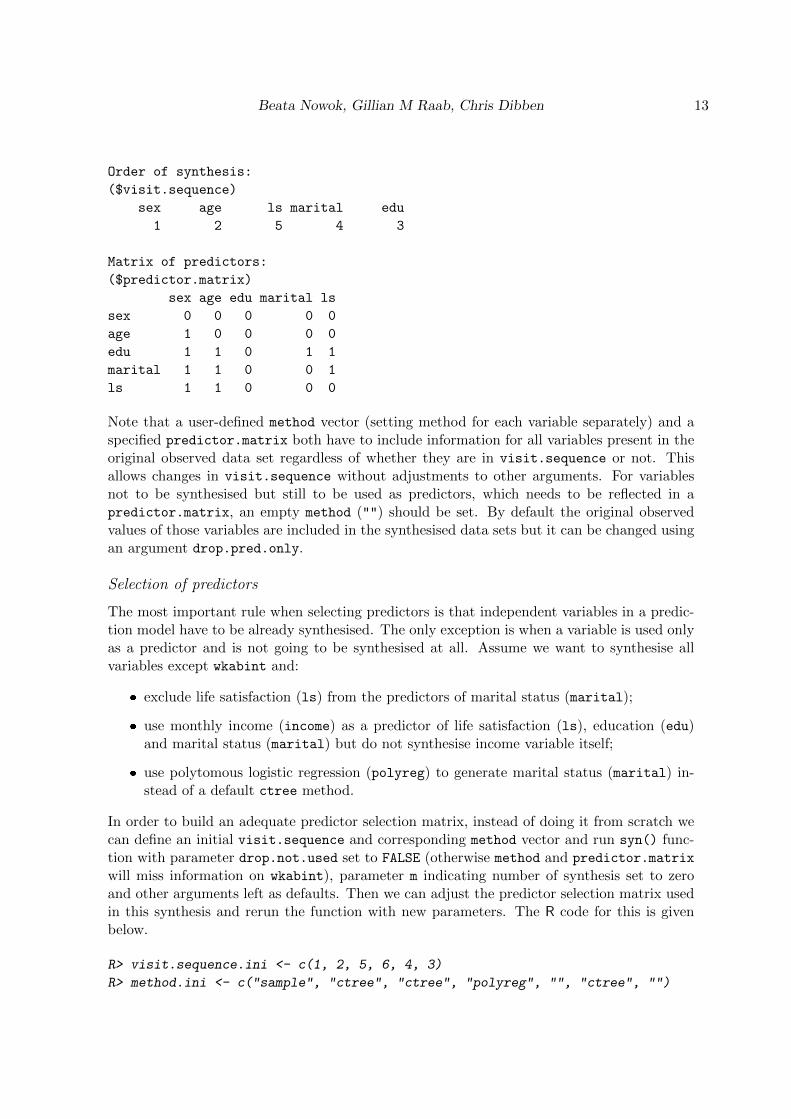
Beata Nowok, Gillian M Raab, Chris Dibben 13

Order of synthesis:

($visit.sequence)

sex age ls marital edu

1 2 5 4 3

Matrix of predictors:

($predictor.matrix)

sex age edu marital ls

sex 0 0 0 0 0

age 1 0 0 0 0

edu 1 1 0 1 1

marital 1 1 0 0 1

ls 1 1 0 0 0

Note that a user-defined method vector (setting method for each variable separately) and aspecified predictor.matrix both have to include information for all variables present in theoriginal observed data set regardless of whether they are in visit.sequence or not. Thisallows changes in visit.sequence without adjustments to other arguments. For variablesnot to be synthesised but still to be used as predictors, which needs to be reflected in apredictor.matrix, an empty method ("") should be set. By default the original observedvalues of those variables are included in the synthesised data sets but it can be changed usingan argument drop.pred.only.

Selection of predictors

The most important rule when selecting predictors is that independent variables in a predic-tion model have to be already synthesised. The only exception is when a variable is used onlyas a predictor and is not going to be synthesised at all. Assume we want to synthesise allvariables except wkabint and:

� exclude life satisfaction (ls) from the predictors of marital status (marital);

� use monthly income (income) as a predictor of life satisfaction (ls), education (edu)and marital status (marital) but do not synthesise income variable itself;

� use polytomous logistic regression (polyreg) to generate marital status (marital) in-stead of a default ctree method.

In order to build an adequate predictor selection matrix, instead of doing it from scratch wecan define an initial visit.sequence and corresponding method vector and run syn() func-tion with parameter drop.not.used set to FALSE (otherwise method and predictor.matrix

will miss information on wkabint), parameter m indicating number of synthesis set to zeroand other arguments left as defaults. Then we can adjust the predictor selection matrix usedin this synthesis and rerun the function with new parameters. The R code for this is givenbelow.

R> visit.sequence.ini <- c(1, 2, 5, 6, 4, 3)

R> method.ini <- c("sample", "ctree", "ctree", "polyreg", "", "ctree", "")

14 synthpop: Synthetic Populations in R

R> sds.ini <- syn(data = ods, visit.sequence = visit.sequence.ini,

+ method = method.ini, m = 0, drop.not.used = FALSE)

R> sds.ini$predictor.matrix

sex age edu marital income ls wkabint

sex 0 0 0 0 0 0 0

age 1 0 0 0 0 0 0

edu 1 1 0 1 1 1 0

marital 1 1 0 0 1 1 0

income 0 0 0 0 0 0 0

ls 1 1 0 0 1 0 0

wkabint 0 0 0 0 0 0 0

R> predictor.matrix.corrected <- sds.ini$predictor.matrix

R> predictor.matrix.corrected["marital", "ls"] <- 0

R> predictor.matrix.corrected

sex age edu marital income ls wkabint

sex 0 0 0 0 0 0 0

age 1 0 0 0 0 0 0

edu 1 1 0 1 1 1 0

marital 1 1 0 0 1 0 0

income 0 0 0 0 0 0 0

ls 1 1 0 0 1 0 0

wkabint 0 0 0 0 0 0 0

R> sds.corrected <- syn(data = ods, visit.sequence = visit.sequence.ini,

+ method = method.ini, predictor.matrix = predictor.matrix.corrected,

+ seed = my.seed)

Handling missing values in continuous variables

Data can be missing for a number of reasons (e.g. refusal, inapplicability, lack of knowledge)and multiple missing data codes are used to represent this variety. By default, numericmissing data codes for a continuous variable are treated as non-missing values. This maylead to erroneous synthetic values, especially when standard parametric models are used orwhen synthetic values are smoothed to decrease disclosure risk. The problem refers not onlyto the variable in question, but also to variables predicted from it. The parameter cont.na

of the syn() function allows to define missing-data codes for continuous variables in order tomodel them separately (see Section 3.2). In our simple example a continuous variable income

has two types of missing values (NA and -8) and they should be provided in a list elementnamed "income". The following code shows the recommended settings for synthesis of incomevariable, which includes smoothing and separate synthesis of missing values

R> sds.income <- syn(ods, cont.na = list(income = c(NA, -8)),

+ smoothing = list(income = "density"), seed = NA)

Beata Nowok, Gillian M Raab, Chris Dibben 15

Rules for restricted values

To illustrate application of rules for restricted values consider marital status. According toPolish law males have to be at least 18 to get married. Thus, in our synthesised data setall male individuals younger than 18 should have marital status SINGLE which is the case inthe observed data set. Running without rules gives incorrect results with some of the malesunder 18 classified as MARRIED (see summary output table below).

R> M18.ods <- table(subset(ods,

+ age < 18 & sex == "MALE", marital))

R> M18.default <- table(subset(sds.default$syn,

+ age < 18 & sex == "MALE", marital))

R> M18.parametric <- table(subset(sds.parametric$syn,

+ age < 18 & sex == "MALE", marital))

R> cbind("Observed data" = M18.ods, CART = M18.default,

+ Parametric = M18.parametric)

Observed data CART Parametric

SINGLE 57 56 49

MARRIED 0 2 3

WIDOWED 0 0 0

DIVORCED 0 0 0

LEGALLY SEPARATED 0 0 0

DE FACTO SEPARATED 0 0 0

Application of a rule, as specified below using named lists, leads to the correct results

R> rules.marital <- list(marital = "age < 18 & sex == 'MALE'")

R> rvalues.marital <- list(marital = "SINGLE")

R> sds.rmarital <- syn(ods, rules = rules.marital,

+ rvalues = rvalues.marital, seed = my.seed)

R> sds.rmarital.param <- syn(ods, rules = rules.marital,

+ rvalues = rvalues.marital, method = "parametric", seed = my.seed)

A summary table can be produced using the following code

R> rM18.default <- table(subset(sds.rmarital$syn,

+ age < 18 & sex == "MALE", marital))

R> rM18.parametric <- table(subset(sds.rmarital.param$syn,

+ age < 18 & sex == "MALE", marital))

R> cbind("Observed data" = M18.ods, CART = rM18.default,

+ Parametric = rM18.parametric)

Observed data CART Parametric

SINGLE 57 58 52

MARRIED 0 0 0

WIDOWED 0 0 0

16 synthpop: Synthetic Populations in R

DIVORCED 0 0 0

LEGALLY SEPARATED 0 0 0

DE FACTO SEPARATED 0 0 0

4.4. Synthetic data analysis

Ideally, if the models used for synthesis truly represents the process that generated the originalobserved data, an analysis based on the synthesised data should lead to the same statisticalinferences as an analysis based on the actual data. For illustration we estimate here a simplelogistic regression model where our dependent variable is a probability of intention to workabroad. We use the wkabint variable which specifies the intentions of work migration but weadjust it to disregard the destination country group. Besides we recode the current missingdata code of variable income (-8) into the R missing data code NA.

R> ods$wkabint <- as.character(ods$wkabint)

R> ods$wkabint[ods$wkabint == "YES, TO EU COUNTRY" |

+ ods$wkabint == "YES, TO NON-EU COUNTRY"] <- "YES"

R> ods$wkabint <- factor(ods$wkabint)

R> ods$income[ods$income == -8] <- NA

We generate five synthetic data sets.

R> sds <- syn(ods, method = "ctree", m = 5, seed = my.seed)

Before running the models let us compare some descriptive statistics of the observed andsynthetic data sets. A very useful function in R for this purpose is summary(). When adata frame is provided as an argument, here our original data set ods, it produces summarystatistics of each variable.

R> summary(ods)

sex age edu

MALE :2182 Min. :16.0 PRIMARY/NO EDUCATION : 962

FEMALE:2818 1st Qu.:32.0 VOCATIONAL/GRAMMAR :1613

Median :49.0 SECONDARY :1482

Mean :47.7 POST-SECONDARY OR HIGHER: 936

3rd Qu.:61.0 NA's : 7

Max. :97.0

marital income ls

SINGLE :1253 Min. : 100 PLEASED :1947

MARRIED :2979 1st Qu.: 970 MOSTLY SATISFIED :1692

WIDOWED : 531 Median : 1350 MIXED : 827

DIVORCED : 199 Mean : 1641 MOSTLY DISSATISFIED: 274

LEGALLY SEPARATED : 7 3rd Qu.: 2000 DELIGHTED : 191

DE FACTO SEPARATED: 22 Max. :16000 (Other) : 61

Beata Nowok, Gillian M Raab, Chris Dibben 17

NA's : 9 NA's :1286 NA's : 8

wkabint

NO :4646

YES : 318

NA's: 36

The summary() function with the synds object as an argument gives summary statistics of thevariables in the synthesised data set. If more than one synthetic data set has been generated,as default summaries are calculated by averaging summary values for all synthetic data copies.

R> summary(sds)

Synthetic object with 5 syntheses using methods:

sex age edu marital income ls wkabint

"sample" "ctree" "ctree" "ctree" "ctree" "ctree" "ctree"

Summary (average) for all synthetic data sets:

sex age edu

MALE :2169 Min. :16.0 PRIMARY/NO EDUCATION : 964.0

FEMALE:2831 1st Qu.:32.0 VOCATIONAL/GRAMMAR :1593.6

Median :48.6 SECONDARY :1501.4

Mean :47.8 POST-SECONDARY OR HIGHER: 935.8

3rd Qu.:61.6 NA's : 5.2

Max. :95.6

marital income ls

SINGLE :1246.0 Min. : 100 PLEASED :1964.4

MARRIED :2986.2 1st Qu.: 955 MOSTLY SATISFIED :1672.6

WIDOWED : 543.6 Median : 1310 MIXED : 836.8

DIVORCED : 187.2 Mean : 1632 MOSTLY DISSATISFIED: 281.6

LEGALLY SEPARATED : 6.8 3rd Qu.: 2000 DELIGHTED : 179.4

DE FACTO SEPARATED: 21.2 Max. :15600 (Other) : 56.4

NA's : 9.0 NA's : 1260 NA's : 8.8

wkabint

NO :4634.8

YES : 330.4

NA's: 34.8

Summary of individual data sets can be displayed by supplying the msel parameter, whichcan be a single number or a vector with selected synthesis numbers. An example code ispresented below but the corresponding output is suppressed for space reasons.

R> summary(sds, msel = 2)

R> summary(sds, msel = 1:5)

To compare the synthesised variables with the original ones more easily, the synthesiser can usea compare() function. It is a generic function for comparison of various aspects of synthesised

18 synthpop: Synthetic Populations in R

income

0

10

20

30

0 10002000

30004000

50006000

70008000

900010000

1100012000

1300014000

15000miss.NA

Value

Per

cent

observed synthetic

Figure 1: Relative frequency distribution of non-missing values and missing data categoriesfor income variable for observed and synthetic data.

and observed data. The function invokes particular methods depending on the class of thefirst argument. If a synthetic data object and a data frame with original data are provided itcompares relative frequency distributions of each variable in tabular and graphic form. Thenumber of plots per page can be specified via nrow and ncol arguments. Alternatively, thefunction can be used for a subset of variables specified by a vars argument. Output for incomeis presented below and in Figure 1. For quantitative variables, such as income, missing datacategories are plotted on the same plot as non-missing values and they are indicated by miss.

suffix. If a synthetic data object contains multiple data sets by default pooled synthetic dataare used for comparison.

R> compare(sds, ods, vars = "income")

Comparing percentages observed with synthetic

$income

0 1000 2000 3000 4000 5000 6000 7000 8000 9000 10000

observed 24.58 34.98 9.440 2.66 1.360 0.480 0.260 0.20 0.080 0.10 0.040

synthetic 25.33 34.66 9.472 2.66 1.448 0.484 0.336 0.16 0.044 0.06 0.036

11000 12000 13000 14000 15000 miss.NA

observed 0.02 0 0 0.060 0.020 25.72

synthetic 0.02 0 0 0.076 0.012 25.20

An argument msel can be used to compare the observed data with a single or multiple

Beata Nowok, Gillian M Raab, Chris Dibben 19

individual synthetic data sets, which is illustrated below and in Figure 2 for a life satisfactionfactor variable (ls).

R> compare(sds, ods, vars = "ls", msel = 1:3)

Comparing percentages observed with synthetic

$ls

DELIGHTED PLEASED MOSTLY SATISFIED MIXED MOSTLY DISSATISFIED

observed 3.82 38.94 33.84 16.54 5.48

syn=1 3.54 38.78 33.44 17.22 5.76

syn=2 3.62 39.34 33.44 16.68 5.72

syn=3 3.66 38.92 34.34 16.66 5.14

UNHAPPY TERRIBLE <NA>

observed 0.82 0.40 0.16

syn=1 0.66 0.44 0.16

syn=2 0.66 0.20 0.34

syn=3 0.74 0.44 0.10

ls

0

10

20

30

40

DELIGHTED

PLEASED

MOSTLY SATISFIED

MIXEDMOSTLY DISSATISFIED

UNHAPPY

TERRIBLE

NA

Value

Per

cent

observed syn=1 syn=2 syn=3

Figure 2: Relative frequency distribution of life satisfaction (ls) for observed and syntheticdata.

Returning to the logistic regression model for wkabint, we estimate the original data model us-ing generalised linear models implemented in R glm() function. A synthpop package function

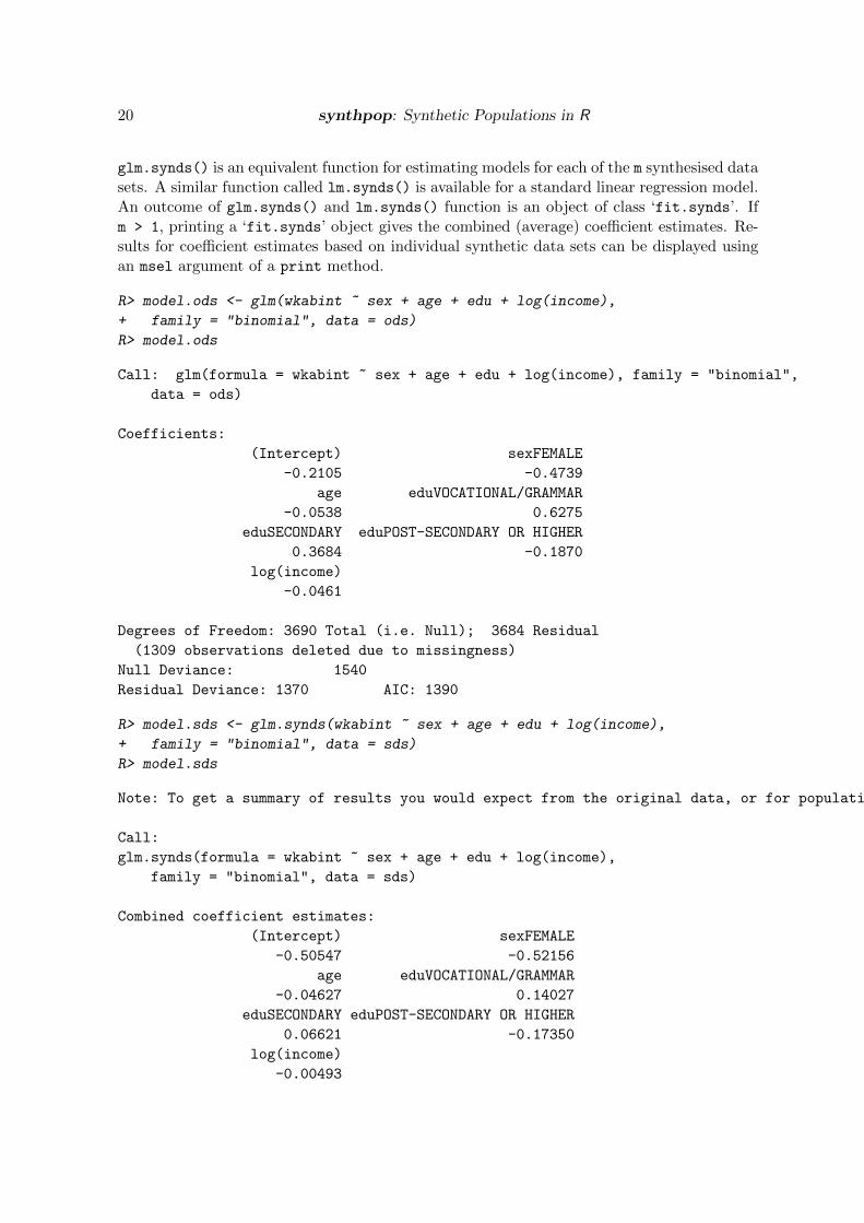
20 synthpop: Synthetic Populations in R

glm.synds() is an equivalent function for estimating models for each of the m synthesised datasets. A similar function called lm.synds() is available for a standard linear regression model.An outcome of glm.synds() and lm.synds() function is an object of class ‘fit.synds’. Ifm > 1, printing a ‘fit.synds’ object gives the combined (average) coefficient estimates. Re-sults for coefficient estimates based on individual synthetic data sets can be displayed usingan msel argument of a print method.

R> model.ods <- glm(wkabint ~ sex + age + edu + log(income),

+ family = "binomial", data = ods)

R> model.ods

Call: glm(formula = wkabint ~ sex + age + edu + log(income), family = "binomial",

data = ods)

Coefficients:

(Intercept) sexFEMALE

-0.2105 -0.4739

age eduVOCATIONAL/GRAMMAR

-0.0538 0.6275

eduSECONDARY eduPOST-SECONDARY OR HIGHER

0.3684 -0.1870

log(income)

-0.0461

Degrees of Freedom: 3690 Total (i.e. Null); 3684 Residual

(1309 observations deleted due to missingness)

Null Deviance: 1540

Residual Deviance: 1370 AIC: 1390

R> model.sds <- glm.synds(wkabint ~ sex + age + edu + log(income),

+ family = "binomial", data = sds)

R> model.sds

Note: To get a summary of results you would expect from the original data, or for population inference use the summary function on your fit.

Call:

glm.synds(formula = wkabint ~ sex + age + edu + log(income),

family = "binomial", data = sds)

Combined coefficient estimates:

(Intercept) sexFEMALE

-0.50547 -0.52156

age eduVOCATIONAL/GRAMMAR

-0.04627 0.14027

eduSECONDARY eduPOST-SECONDARY OR HIGHER

0.06621 -0.17350

log(income)

-0.00493

Beata Nowok, Gillian M Raab, Chris Dibben 21

The summary() function of a fit.synds object can be used by the analyst to combineestimates based on all the synthesised data sets. By default inference is made to orig-inal data quantities. In order to make inference to population quantities the parameterpopulation.inference has to be set to TRUE. The function’s result provides point estimatesof coefficients (B.syn), their standard errors (se(B.syn)) and Z scores (Z.syn) for populationand observed data quantities respectively. For inference to original data quantities it containsin addition estimates of the actual standard errors based on synthetic data (se(Beta).syn)and standard errors of Z scores (se(Z.syn)). Note that not all these quantities are printedautomatically.

The mean of the estimates from each of the m synthetic data sets yields unbiased estimatesof the coefficients if the data conform to the model used for synthesis. The variance isestimated differently depending whether inference is made to the original data quantities orthe population parameters and whether synthetic data were produced using simple or propersynthesis (for details see Raab et al. 2016; expressions used to calculate variance for differentcases are presented in Table 1). By default a simple synthesis is conducted and inference ismade to original data quantities.

R> summary(model.sds)

Warning: Note that all these results depend on the synthesis model being correct.

Fit to synthetic data set with 5 syntheses.

Inference to coefficients and standard errors that

would be obtained from the observed data.

Call:

glm.synds(formula = wkabint ~ sex + age + edu + log(income),

family = "binomial", data = sds)

Combined estimates:

xpct(Beta) xpct(se.Beta) xpct(z) Pr(>|xpct(z)|)

(Intercept) -0.50547 0.98440 -0.51 0.60761

sexFEMALE -0.52156 0.15807 -3.30 0.00097

age -0.04627 0.00524 -8.83 < 2e-16

eduVOCATIONAL/GRAMMAR 0.14027 0.26764 0.52 0.60020

eduSECONDARY 0.06621 0.27579 0.24 0.81029

eduPOST-SECONDARY OR HIGHER -0.17350 0.31212 -0.56 0.57829

log(income) -0.00493 0.13049 -0.04 0.96986

(Intercept)

sexFEMALE ***

age ***

eduVOCATIONAL/GRAMMAR

eduSECONDARY

eduPOST-SECONDARY OR HIGHER

log(income)

22 synthpop: Synthetic Populations in R

---

Signif. codes: 0 '***' 0.001 '**' 0.01 '*' 0.05 '.' 0.1 ' ' 1

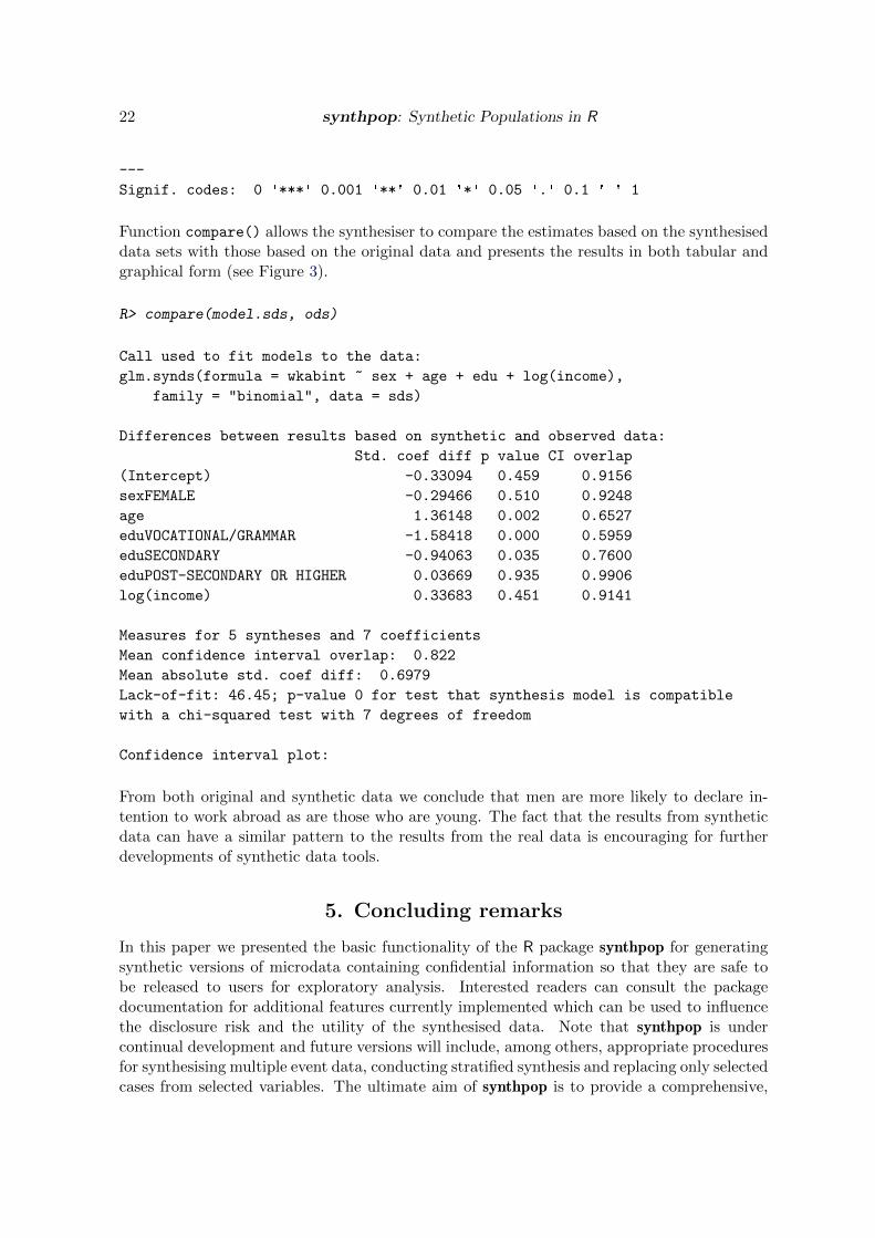
Function compare() allows the synthesiser to compare the estimates based on the synthesiseddata sets with those based on the original data and presents the results in both tabular andgraphical form (see Figure 3).

R> compare(model.sds, ods)

Call used to fit models to the data:

glm.synds(formula = wkabint ~ sex + age + edu + log(income),

family = "binomial", data = sds)

Differences between results based on synthetic and observed data:

Std. coef diff p value CI overlap

(Intercept) -0.33094 0.459 0.9156

sexFEMALE -0.29466 0.510 0.9248

age 1.36148 0.002 0.6527

eduVOCATIONAL/GRAMMAR -1.58418 0.000 0.5959

eduSECONDARY -0.94063 0.035 0.7600

eduPOST-SECONDARY OR HIGHER 0.03669 0.935 0.9906

log(income) 0.33683 0.451 0.9141

Measures for 5 syntheses and 7 coefficients

Mean confidence interval overlap: 0.822

Mean absolute std. coef diff: 0.6979

Lack-of-fit: 46.45; p-value 0 for test that synthesis model is compatible

with a chi-squared test with 7 degrees of freedom

Confidence interval plot:

From both original and synthetic data we conclude that men are more likely to declare in-tention to work abroad as are those who are young. The fact that the results from syntheticdata can have a similar pattern to the results from the real data is encouraging for furtherdevelopments of synthetic data tools.

5. Concluding remarks

In this paper we presented the basic functionality of the R package synthpop for generatingsynthetic versions of microdata containing confidential information so that they are safe tobe released to users for exploratory analysis. Interested readers can consult the packagedocumentation for additional features currently implemented which can be used to influencethe disclosure risk and the utility of the synthesised data. Note that synthpop is undercontinual development and future versions will include, among others, appropriate proceduresfor synthesising multiple event data, conducting stratified synthesis and replacing only selectedcases from selected variables. The ultimate aim of synthpop is to provide a comprehensive,

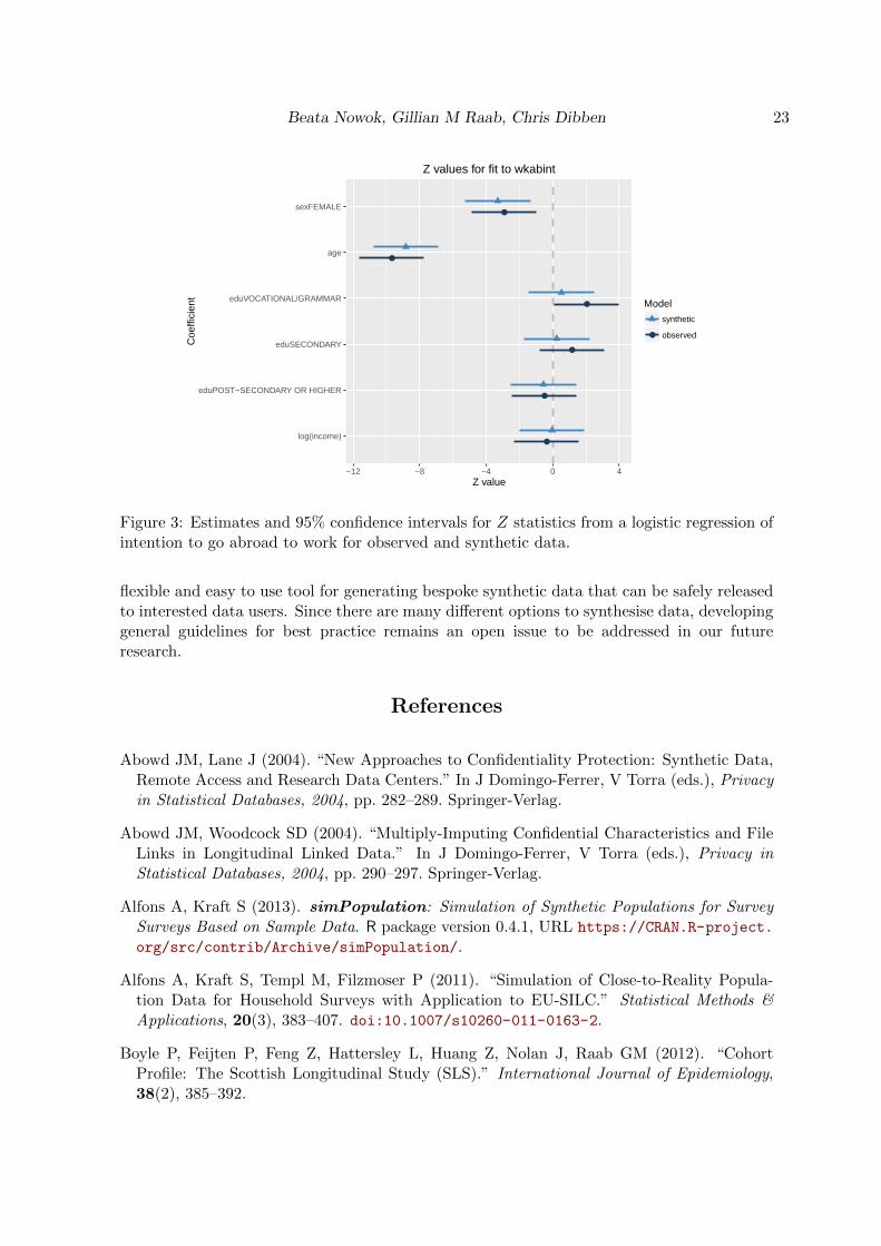
Beata Nowok, Gillian M Raab, Chris Dibben 23

●

●

●

●

●

●

log(income)

eduPOST−SECONDARY OR HIGHER

eduSECONDARY

eduVOCATIONAL/GRAMMAR

age

sexFEMALE

−12 −8 −4 0 4Z value

Coe

ffici

ent

Model

●

synthetic

observed

Z values for fit to wkabint

Figure 3: Estimates and 95% confidence intervals for Z statistics from a logistic regression ofintention to go abroad to work for observed and synthetic data.

flexible and easy to use tool for generating bespoke synthetic data that can be safely releasedto interested data users. Since there are many different options to synthesise data, developinggeneral guidelines for best practice remains an open issue to be addressed in our futureresearch.

References

Abowd JM, Lane J (2004). “New Approaches to Confidentiality Protection: Synthetic Data,Remote Access and Research Data Centers.” In J Domingo-Ferrer, V Torra (eds.), Privacyin Statistical Databases, 2004, pp. 282–289. Springer-Verlag.

Abowd JM, Woodcock SD (2004). “Multiply-Imputing Confidential Characteristics and FileLinks in Longitudinal Linked Data.” In J Domingo-Ferrer, V Torra (eds.), Privacy inStatistical Databases, 2004, pp. 290–297. Springer-Verlag.

Alfons A, Kraft S (2013). simPopulation: Simulation of Synthetic Populations for SurveySurveys Based on Sample Data. R package version 0.4.1, URL https://CRAN.R-project.

org/src/contrib/Archive/simPopulation/.

Alfons A, Kraft S, Templ M, Filzmoser P (2011). “Simulation of Close-to-Reality Popula-tion Data for Household Surveys with Application to EU-SILC.” Statistical Methods &Applications, 20(3), 383–407. doi:10.1007/s10260-011-0163-2.

Boyle P, Feijten P, Feng Z, Hattersley L, Huang Z, Nolan J, Raab GM (2012). “CohortProfile: The Scottish Longitudinal Study (SLS).” International Journal of Epidemiology,38(2), 385–392.

24 synthpop: Synthetic Populations in R

Breiman L, Friedman JH, Olshen RA, Stone CJ (1984). Classification and Regression Trees.Belmont, Wadsworth.

Caiola G, Reiter JP (2010). “Random Forests for Generating Partially Synthetic, CategoricalData.” Transactions on Data Privacy, 3(1), 27–42.

Council for Social Monitoring (2011). “Social Diagnosis 2000–2011: Integrated Database.”URL http://www.diagnoza.com/index-en.html.

Drechsler J (2011). Synthetic Data Sets for Statistical Disclosure Control. Springer-Verlag.doi:10.1007/978-1-4614-0326-5.

Drechsler J, Reiter JP (2010). “Sampling with Synthesis: A New Approach for ReleasingPublic Use Census Microdata.” Journal of the American Statistical Association, 105(492),1347–1357. doi:10.1198/jasa.2010.ap09480.

Drechsler J, Reiter JP (2011). “An Empirical Evaluation of Easily Implemented, Nonparamet-ric Methods for Generating Synthetic Datasets.” Computational Statistics & Data Analysis,55(12), 3232–3243. doi:10.1016/j.csda.2011.06.006.

Elliot M (2015). “Final Report on the Disclosure Risk Associated with the Synthetic DataProduced by the SYLLS Team.” Report 2015-2, Cathie Marsh Institute for Social Re-search (CMIST), University of Manchester. URL http://www.cmist.manchester.ac.uk/

research/publications/reports.

Elliot M, Purdam K (2007). “A Case Study of the Impact of Statistical Disclosure Controlon Data Quality in the Individual UK Samples of Anonymized Records.” Environment andPlanning A, 39(5), 1101–1118. doi:10.1068/a38335.

Hattersley L, Cresser R (1995). “Longitudinal Study, 1971–1991: History, Organisation andQuality of Data.” LS Series 7, HMSO, London. URL http://celsius.lshtm.ac.uk/

documents/LS%20No.7%20Hattersley%20&%20Creeser%201995.pdf.

Hothorn T, Hornik K, Zeileis A (2006). “Unbiased Recursive Partitioning: A ConditionalInference Framework.” Journal of Computational and Graphical Statistics, 15(3), 651–674.doi:10.1198/106186006x133933.

Kinney SK, Reiter JP, Berger JO (2010). “Model Selection When Multiple Imputation is Usedto Protect Confidentiality in Public Use Data.” Journal of Privacy and Confidentiality, 2(2),3–19.

Kinney SK, Reiter JP, Reznek AP, Miranda J, Jarmin RS, Abowd JM (2011). “Towards Un-restricted Public Use Business Microdata: The Synthetic Longitudinal Business Database.”International Statistical Review, 79(3), 362–384. doi:10.1111/j.1751-5823.2011.00153.x.

Little RJA (1993). “Statistical Analysis of Masked Data.” Journal of Official Statistics, 9(2),407–26.

Meindl B, Templ M, Alfons A, Kowarik A (2016). simPop: Simulation of Synthetic Popu-lations for Survey Data Considering Auxiliary Information. R package version 0.3.0, URLhttps://CRAN.R-project.org/package=simPop.

Beata Nowok, Gillian M Raab, Chris Dibben 25

Nowok B, Raab GM, Snoke J, Dibben C (2016). synthpop: Generating Synthetic Versionsof Sensitive Microdata for Statistical Disclosure Control. R package version 1.3-0, URLhttps://CRAN.R-project.org/package=synthpop.

Ohm P (2010). “Broken Promises of Privacy: Responding to the Surprising Failure ofAnonymization.” UCLA Law Review, 57(6), 1701–1775.

O’Reilly D, Rosato M, Catney G, Johnston F, Brolly M (2011). “Cohort Description: TheNorthern Ireland Longitudinal Study (NILS).” International Journal of Epidemiology,41(3), 634–641.

Raab GM, Nowok B, Dibben C (2016). “Practical Data Synthesis for Large Samples.”arXiv:1409.0217 [stat.ME], URL http://arxiv.org/abs/1409.0217.

Raghunathan TE, Reiter JP, Rubin DB (2003). “Multiple Imputation for Statistical DisclosureLimitation.” Journal of Official Statistics, 19(1), 1–17.

Raghunathan TE, Solenberger PW, Van Hoewyk J (2002). “IVEware: Imputation andVariance Estimation Software User Guide.” Technical report, Survey Methodology Pro-gram, Survey Research Center, Institute for Social Research, University of Michigan. URLhttp://www.isr.umich.edu/src/smp/ive/.

R Core Team (2016). R: A Language and Environment for Statistical Computing. R Founda-tion for Statistical Computing, Vienna, Austria. URL https://www.R-project.org/.

Reiter JP (2002). “Satisfying Disclosure Restrictions with Synthetic Data Sets.” Journal ofOfficial Statistics, 18(4), 531–544.

Reiter JP (2003). “Inference for Partially Synthetic, Public Use Microdata Sets.” SurveyMethodology, 29(2), 181–188.

Reiter JP (2005a). “Releasing Multiply Imputed, Synthetic Public Use Microdata: An Illus-tration and Empirical Study.” Journal of the Royal Statistical Society A, 168(1), 185–205.doi:10.1111/j.1467-985x.2004.00343.x.

Reiter JP (2005b). “Using CART to Generate Partially Synthetic, Public Use Microdata.”Journal of Official Statistics, 21(3), 441–462.

Reiter JP, Kinney SK (2012). “Inferentially Valid, Partially Synthetic Data: Generating fromPosterior Predictive Distributions Not Necessary.” Journal of Official Statistics, 28(4),583–590.

Reiter JP, Raghunathan E (2007). “The Multiple Adaptations of Multiple Imputa-tion.” Journal of the American Statistical Society, 102(480), 1462–1471. doi:10.1198/

016214507000000932.

Rubin DB (1993). “Discussion: Statistical Disclosure Limitation.” Journal of Official Statis-tics, 9(2), 461–468.

SAS Institute Inc (2013). SAS Software, Version 9.4. Cary. URL http://www.sas.com/.

26 synthpop: Synthetic Populations in R

Survey Methodology Program (2011). “IVEware: Imputation and Variance Estimation Ver-sion 0.2 Users Guide (Supplement).” Technical report, Survey Research Center, Institutefor Social Research, University of Michigan. URL http://www.isr.umich.edu/src/smp/

ive/.

Therneau T, Atkinson B, Ripley B (2015). rpart: Recursive Partitioning and RegressionTrees. R package version 4.1-10, URL https://CRAN.R-project.org/package=rpart.

Van Buuren S, Groothuis-Oudshoorn K (2011). “mice: Multivariate Imputation by ChainedEquations in R.” Journal of Statistical Software, 45(3), 1–67. doi:10.18637/jss.v045.

i03.

Winkler WE (2007). “Examples of Easy-to-Implement, Widely Used Methods of Maskingfor Which Analytical Properties Are Not Justified.” Technical Report Series 21, Statisti-cal Research Division, U.S. Census Bureau, Washington. URL http://www.census.gov.

edgekey.net/srd/papers/pdf/rrs2007-21.pdf.

Affiliation:

Beata NowokInstitute of GeographySchool of GeoSciencesUniversity of EdinburghDrummond StreetEdinburgh EH8 9XP, United KingdomE-mail: beata.nowok@ed.ac.uk