Synthetic estimation of healthy lifestyles indicators...

Synthetic estimation of healthylifestyles indicators:Stage 1 reportMadhavi Bajekal, Shaun Scholes, Kevin Pickering, Susan Purdon

Synthetic estimation of healthylifestyles indicators: Stage 1 reportMadhavi Bajekal, Shaun Scholes, Kevin Pickering, Susan Purdon

Prepared for the Department of Health

May 2004

Contents

Summary......................................................................................................................3

1 INTRODUCTION..............................................................................................61.1 Overall aims of the project.............................................................................. 61.2 This report......................................................................................................... 6

2 REVIEW OF LITERATURE..............................................................................82.1 What is synthetic estimation and why it is needed..................................... 82.2 Typology of methods ...................................................................................... 82.3 Simple methods................................................................................................ 9

2.3.1 Indirect standardisation ..............................................................................92.3.2 Strengths and limitations ............................................................................9

2.4 Models using individual level covariates only.......................................... 102.4.1 Using covariates from the Census ...........................................................102.4.2 Using covariates from SARs.....................................................................112.4.3 Strengths and limitations ..........................................................................11

2.5 Models combining individual and area level covariates ......................... 112.5.1 Strengths and limitations ..........................................................................12

2.6 Models using area level covariates only..................................................... 132.6.1 Strengths and limitations ..........................................................................14

2.7 Other approaches for larger geographical areas ....................................... 152.7.1 GREG estimator .........................................................................................152.7.2 Composite estimators................................................................................162.7.3 Fay-Herriot estimator ................................................................................16

2.8 Summary of methods at the ward level...................................................... 17

3 SCOPING AND SETTING UP THE DATABASE.....................................193.1 Data requirements ......................................................................................... 193.2 Geographical matching ................................................................................. 203.3 Survey dataset ................................................................................................ 21

Sample size and spatial coverage ..................................................................21Sample-based individual-level covariates .....................................................22

3.4 Area-level covariate dataset ......................................................................... 233.4.1 Ward level covariates ................................................................................23

Census data...................................................................................................23Administrative data......................................................................................24

3.4.2 Higher-area level covariates.....................................................................243.4.3 Covariates at other geographies ..............................................................24

3.5 Validation dataset .......................................................................................... 25

4 CALCULATION OF CONFIDENCE INTERVALS FOR SYNTHETICESTIMATES ......................................................................................................26

4.1.1 Confidence intervals derived from the model estimates......................264.1.2 Confidence/credible intervals estimated by simulation ......................27

4.2 Indicative confidence intervals for wards .................................................. 274.3 Calculation of confidence intervals for aggregated synthetic estimates 28

5 TESTING THE SOFTWARE..........................................................................29

National Centre for Social Research

1

6 RECOMMENDATIONS FOR STAGE 2 .....................................................306.1 Choice of estimation area.............................................................................. 306.2 Which models to test? ................................................................................... 316.3 Which health measures? ............................................................................... 316.4 Proposed approach to model validation .................................................... 326.5 User engagement ........................................................................................... 33

REFERENCES ...........................................................................................................34


2

Acknowledgements

We would like to thank members of the Steering Group and the Technical Group fortheir helpful comments on this report. We are grateful to Prof Graham Moon and DrLiz Twigg (University of Portsmouth) and Patrick Heady (ONS) for discussing theirprevious work on this topic with us. Colleagues at the Survey Methods Unit(NatCen) contributed generously of their time in developing and refiningmethodology through regular seminar discussions. We would particularly like toexpress our appreciation of the work of Department of Health staff at all stages of theproject and in particular the contribution made by Rosemary Aldridge, Tracie Kilbey,David Greeno, Bill Hageman and Seb Morton-Clark.


3

Summary

Aims and objectivesThe aim of the synthetic estimation project is to provide robust estimates of healthcharacteristics and behaviours of populations for all small areas in England tosupport comparisons within and between local areas such as Local AuthorityDistricts and Primary Care Organisations.

Synthetic estimation can be defined as the application of model-based techniques tocombine data obtained from national surveys (containing the health behaviourmeasures of interest) with a set of associated covariate (or predictor) variablesavailable for all small areas (e.g. the proportions of residents who were living as acouple, claiming Income Support, had a limiting longstanding illness etc). Thesynthetic estimate generated for a particular small area is the expected outcome forthat area based on its characteristics as measured by the covariate variables. Tointerpret the estimates it is recommended that users adopt statements such as: giventhe characteristics of the local population we would expect approximately x% of adults withinward X to smoke/be obese etc.

This report sets out the findings of the first stage of the project. Stage 1 was a scopingstudy to assess the methodological, technical and data requirements for syntheticestimation in order to inform the work-plan for the next stage (evaluation andtesting) of the project. The main findings and recommendations of the report aresummarised below.

Review of literature The literature review identified four types of methods used for small-area estimation:two (simpler) approaches that have used only individual (or person) level covariatesand therefore adjust solely for the differences in the demographic compositionbetween areas; and two approaches that have used multilevel modelling tosimultaneously take into account the impact of differences in population compositionand the wider social context between small areas. The latter approaches areconceptually more advanced than the simpler methods, but are alsomethodologically and computationally more complex.

Confidence intervals and testing the softwareThe report sets out our approach to generate confidence intervals around estimatesat lower and higher level geographies for the multi-level models. Indicativeconfidence intervals for ward-level estimates were also calculated. Two softwarepackages appropriate for hierarchical modelling were tested to assess processingrequirements and to develop algorithms to speed up the model building process.

Which models to test?The literature review and tests indicated that the two multi-level model methods -namely, the one using area-level covariates only (extensively tested by the ONS), andthe other using covariates measured at both the area and the individual (or person)level – would produce reasonable synthetic estimates and were technically feasible todo. The recommendation of this report is that the two multi-level model methodswill be tested in Stage 2 of the project. In addition, a ‘simple’ model-based estimate


4

would also be constructed to assess how close these estimates are to those generatedusing the more complex models.

Setting up the databaseThe database required for generating synthetic estimates involves combiningtogether data from two sets of sources – survey data (from the Health Survey forEngland 2000 to 2002) containing the target health measures of interest (e.g. smokingstatus) and a covariate dataset with the individual and area-level covariates –matched to a common geography for which estimates are required (estimation areaor lowest geographical unit for which estimates are to be generated).

There were a number of advantages to using survey data pooled over the three mostrecent rounds of the Health Survey for England (HSfE) for modelling. First, estimateswould then be based on the most recent data available; second, the selected yearswould span the 2001 Census (the main source for the covariate data ) therebyminimising potential time-lag errors between different data sources; and last,pooling data over years increased the geographical coverage of areas covered by thesample which would potentially improve the fit of the model.

The availability of area-level covariates from Census and administrative sources wasassessed and an initial core set acquired for inclusion in the database.

Because of time and resource constraints, it was decided to match datasets to acommon geography using appropriate look-up tables rather than develop a true GISdatabase. GIS systems allow greater flexibility in locating data points across time,while look-up tables link data points to a geography fixed in time. The loss offlexibility in the database structure meant that re-combining estimates to newboundaries as they change over time will not be feasible. Choice of estimation areaCensus 2001 wards were selected as the smallest estimation area for the project. Themain reason for choosing wards over lower area units (such as Super Output Areas)were statistical constraints imposed by the survey design. The HSfE sample isclustered within postcode sectors which have roughly the same population size aswards. Previous methodological research has shown that because of the similarity insize between the two, the variance between postcode sectors provides reasonablyaccurate variance estimates ( and hence confidence intervals) at ward level but notfor smaller areas. Additionally, a wider range of covariates were available for wardscompared with smaller area levels and previous work had shown that ward levelsynthetic estimates were fairly robust.

Which health behaviour measures?Of the available and policy-relevant health measures included in the HSfE, threehealth measures were recommended for testing in Stage 2 of the project. These arethe prevalence of cigarette smoking among adults, the prevalence of obesity amongadults and the proportion of children aged 5-15 consuming five or more portions offruit and vegetables a day. The selection of target health measures was based on anumber of factors aimed to test the applicability of the methodology for different


5

types of outcomes, namely: outcomes for which good covariate data were available(smoking); health measures with a low measurement error (obesity); and estimatesfor a subgroup of the population (aged 5-15).

In preparation for the next stage of the project, proposals for model testing andvalidation have also been outlined in the report. Model validation will include bothinternal diagnostics of model fit and performance as well as ‘plausibility’ checksagainst external sources of data. The process of identifying suitable data sources forexternal validation has also begun and will continue over Stage 2 of the project.

A key element of the project is to involve users in all stages of the project, fromidentifying information needs and priorities in Stage 1 to taking an active role inlocal validation and dissemination. Our approach to user engagement in Stages 2and 3 are outlined in Section 6.5 of the report.


6

1 INTRODUCTION

The National Centre for Social Research (NatCen) was commissioned by theDepartment of Health to produce estimates of healthy lifestyle behaviours usingHealth Survey for England (HSfE) data. This report describes the work undertakenfor the first stage (the scoping study) of that project.

1.1 Overall aims of the projectThe main aims of the project are:

- to evaluate the technical feasibility of producing robust small-areaestimates for a range of health indicators;

- to validate model-based estimates against other sources ofinformation and local knowledge;

- to develop and apply a consistent methodology to producesynthetic estimates for small-areas, focusing initially on amaximum of five indicators of healthy lifestyles available from theHSfE.

The key requirement of the synthetic estimation project is to provide robust estimatesthat are calculated on a consistent basis for all areas of the country and which allowmeaningful comparisons within and between local areas.

There were three stages to the project – scoping and feasibility, testing and validation,and implementation. Given the experimental nature of synthetic estimationmethodology at present, it was felt that a staged approach would allow considerationof the technical issues that arise, assessment of the quality of the outputs and ‘fit’with user needs at each stage before proceeding to the next stage.

Our remit is to apply the methods that have been developed, not to develop newestimation techniques. Where possible, we shall build on previous work andincorporate new thinking as it emerges.

1.2 This reportThis report documents the progress made at the end of the first stage of the syntheticestimation project. The first stage was primarily a scoping study to assess themethodological, technical and data requirements for the project in order to informthe project plan for the next (evaluation and testing) stage of the project.

The main objectives of the first stage scoping study were to :• review the literature on synthetic estimation techniques including, where

available, literature on the adequacy and reliability of estimates; • scope data requirements and set up a geographically referenced data base

containing the survey and predictor variables from census and administrativesources;


7

• acquire and test the required software (e.g. STATA and MLwiN);• provide an initial assessment of the precision of estimates (i.e. confidence

intervals) to help inform the viability of using the HSfE for synthetic estimation; • recommend a shortlist of potential health behaviours and selected methods to

test in Stage 2 of the project (technical evaluation). The report is broadly organised around these objectives.

Chapter 6 of the report sets out the recommendations from this feasibility study totake forward to Stage 2 of the project.


8

2 REVIEW OF LITERATURE

2.1 What is synthetic estimation and why it is needed

For any small area containing respondents to a survey such as the Health Survey forEngland (HSfE) a conventional estimator of the prevalence of health-relatedbehaviours, such as the proportion of adults who currently smoke, would beconstructed from the survey data alone. Such conventional estimators suffer fromtwo main limitations (Skinner, 1993). First, prevalence estimates can only becomputed for a subset of all areas (i.e. those areas containing respondents to thesurvey). Second, for those sampled areas the achieved sample size will usually besmall and the estimator will thus have low precision. This low precision will bereflected in rather wide confidence intervals for the survey estimates. Othertechniques are therefore required.

Small area estimation can be defined as the application of model-based techniques tocombine data obtained from national surveys (containing the health behaviourmeasure of interest) with a set of associated covariate (or predictor) variables at smallarea level – generally from the Census – to estimate the prevalence of healthylifestyle behaviours for all small areas. Hence, deriving a model-based estimate foreach area (i.e. not just those areas covered by the survey) consists of two stages.

In the first stage, regression analysis is performed modelling the survey data againstavailable predictors of the health behaviour. This analysis is conducted for the subsetof areas covered by the survey. The output from this first stage is a set of parameterestimates. At the second stage, for each area in the population, the coefficients of thepredictor variables obtained from the first stage model are attached to the identicalset of variables available at the small area level to produce an estimate for the area asa whole.

It is the underlying model, therefore, that enables us to move beyond the selectedareas in the sample to provide information about the characteristics of all areas in thepopulation (Goldstein, 2003). For example, we know from previous research thatsmoking behaviour is associated with social status. So individual NS-SEC (NationalStatistics Socio-Economic Classification) is likely to be included as a predictorvariable in the regression for the first stage of synthetic estimation. The coefficientsfor NS-SEC would then be applied to the equivalent NS-SEC information availablefor all areas in the Census 2001.

2.2 Typology of methods

A number of studies have recently produced small area estimates in the UK, with arange of survey variables including income, labour market participation and healthbehaviours. Five different sets of methods were used to generate these estimates:

- simple (non-modelled) methods using indirect standardisation;


9

- models using individual level covariates only;- models combining individual and area-level covariates; - models using area level covariates only; and- other approaches for larger areas of geography.

In the following sections each of the methods is discussed in turn, setting out theirstrengths and limitations in order to inform the selection of methods for testing in thesecond stage of the project.

2.3 Simple methods

2.3.1 Indirect standardisation

Indirect standardisation involved applying national estimates derived from surveydata to area-level population counts to generate expected area estimates. For example,an indirect estimate for the proportion of men smoking in a particular ward could begenerated as follows. First, the proportion of men smoking in each 5-year age bandnationally would be estimated using HSfE data. Applying these national estimates tothe census counts of men within the same 5-year age band for that ward would givean estimate of the number of men that smoke in that ward, from which theproportion could be estimated by dividing by the total census count of men in thatward. Essentially, therefore, the national prevalence rates for each sub-group areweighted by the proportion of persons in that sub-group in the small area.

A recent study has used this method to calculate the prevalence of heart disease forPCOs within two health areas. HSfE survey data was used to derive nationalprevalence rates by age (7 breaks), sex (2) and social class (6) for self-reportedcirculatory illness. Population counts by age and sex were obtained from practiceregisters and NCP profiler used to allocate counts into proxy social class groups. Theappropriate national rates were then applied to the corresponding cell populationcounts to calculate the expected burden of disease for each PCO (Gibson andAsthana S, 2001). This is, in essence, a (non-modelled) method for deriving age, sexand social class adjusted expected rates, based on the national disease prevalence ratesfor each combination.

2.3.2 Strengths and limitations

There are several reasons why indirect standardisation is appealing. First, themethod has intuitive appeal. As Levy (1979) explains, it seems likely that the meanlevel of many variables in a population is highly related to the distribution in thepopulation of such demographic variables as age, sex and social class. In addition toits intuitive appeal, indirectly standardised methods are generally easy andinexpensive to apply since the cell proportions at the local level are available fromthe Census, and the national estimates for demographic classes are easily obtainablefrom national surveys such as the HSfE.

This method also lends itself to two sorts of enhancements. First, rather thancompute estimates at the national level, one possible option is to ‘fine-tune’ themethod by calculating rates for different types of areas using some form of area


10

classification (e.g. urban/rural, quintiles of deprivation), and apply these to theconstituent small areas in each type (Chesterman et al.). Second, the indirectlystandardised estimates for each small area within a larger area (e.g. wards withinLADs) can be ratio adjusted so that a weighted average of the adjusted small areaestimates equals the direct estimate for the larger area. This adjustment ensuresconsistency between the direct and (aggregated up) indirect estimates for the largerareas.

The major drawback of this method, however, is that it assumes that the nationalrates for each subgroup apply uniformly across all areas. The implication for smallarea estimates is that the method assumes that the differences in health behaviourmeasures between areas are due solely to differences in their demographiccomposition. In other words, it is assumed that if two areas had the samecomposition with respect to the demographic variables used, they would have thesame expected prevalence rates (Schaible, 1996). A large body of research, however,has consistently shown that individual health related behaviour, even within thesame social group, varies by ‘contextual’ factors operating at the area level(Macintyre et al., 1993). To deal with such area differences in health a more complexmodel is needed to effectively capture the variation between areas that exists overand above that due to differences in their demographic composition.

2.4 Models using individual level covariates only

2.4.1 Using covariates from the Census

An extension of the indirect standardisation method is to use the modelledrelationship between individual health behaviour measures obtained from a surveyagainst a set of predictor variables for the same individuals recorded in the survey.Generally the covariates chosen for the model are those that are available as countsfor all small areas (e.g. from the Census).

These models estimate the probability that a person with specific knowncharacteristics (say age, sex and social class) currently smokes, is obese etc. Themodel-based probabilities are then converted into estimated proportions in eachsubgroup defined by the covariates who fall into the relevant health category. Theseproportions are then applied to the covariate counts available from the Census toderive an overall estimate for the small area in much the same way as for indirectstandardisation.

In a recent study, Flowers (2003) used this approach to estimate coronary heartdisease (CHD) prevalence rates at PCO level using HSfE 1998-2000 data. Usinglogistic regression, he estimated the probabilities of reported CHD forage/sex/social class/ethnicity groups. These were then applied to the correspondingCensus 2001 counts for each groups to derive CHD prevalence estimates for PCOswithin a health region.


11

2.4.2 Using covariates from SARs

Surveys collect detailed data on a range of individual characteristics andcircumstances - although the inclusion of more and better survey covariates is likelyto greatly improve the fit of such individual level models, analysts are restricted inthe choice of covariates for synthetic estimation by the requirement to haveequivalent covariate information for all areas.

Censuses also collect a fairly wide range of personal data but concerns to preserveconfidentiality set limits to the number of cross-classifications that are released. Aninnovative approach used by Charlton (1998) was to increase the number ofcovariates he was able to use from the survey data by deriving synthetic estimatesusing the Sample of Anonymised Records (SARs) available for the first time for the1991 Census. The 1991 SARs provided a representative 1% sample of individualcensus records with the full set of individual attributes collected in the Censusavailable for all individuals in the SARs.

Charlton was able to use a wide range of individual covariates at the modelling stagefrom the National Survey of Morbidity in General Practice data. The modelcoefficients were then directly applied to the inhabitants of each SAR area with thespecific combination of characteristics included in the model to obtain syntheticestimates for 278 areas (LADs or groups of LADs).


The major drawback of the individual-level approach concerns its data requirements.This form of synthetic estimation requires an exact correspondence between thecovariates used in the model and data available from the Census or otheradministrative data sources. The limited number of cross-tabulations (or crossclassifications) of socio-demographic information such as age, sex, ethnicity, socialclass available from the Census restricts the choice of predictors in these models. Forexample the most detailed cross-tabulation of counts available at ward level from the1991 Census data which were known to affect health behaviour was banded age andgender by marital status (Twigg et al., 2000). The recent 2001 Census tables offermore finely disaggregated counts (e.g. by age, sex, economic activity andqualifications (CAS32) ); this could improve the accuracy of local estimates derivedusing this approach.

2.5 Models combining individual and area level covariates

The methods discussed so far were all at the individual level. An alternative set ofmodels can be described in terms of multi-level models incorporating random effects(also known as mixed models). Their importance to small area estimation lies in thefact that a random effects specification assumes that significant systematic variationbetween small areas remains after the effects of covariates in the model have beenaccounted for. Such ‘unexplained’ variation is modelled through the addition ofsmall area specific random coefficients to the fixed effects (Saei and Chambers, 2003).


12

Such multilevel models give rise to more complex ways of building a model forhealth behaviour measures; generating small area estimates from these modelparameters and finally calculating the confidence intervals for them.

In addition to their ability to incorporate unexplained variability between areas intothe estimation procedures, there are a number of other reasons why multilevelmodels are suitable for producing synthetic estimates for small areas.

First, multilevel models are suited to the clustered nature of social surveys for whichindividuals are clustered within households which in turn are clustered (usually)within postcode sectors. By using the clustering information it provides moreaccurate standard errors, confidence intervals and significance tests, and thesegenerally will be more ‘conservative’ than the traditional estimates obtained byignoring the presence of clustering in the data (Goldstein, 2003). Second, by allowingthe use of covariates measured at any level of the hierarchy, it enables researchers toexplore the extent to which any differences between geographical areas such aswards are associated with individual, household and area level characteristics(Goldstein, 2003).

Using the techniques of multilevel modelling, a model can be applied to survey datathat simultaneously accounts for both individual and area level influences on healthrelated behaviours such as smoking. Twigg et al. (2000) used both individual andarea-level covariates to obtain prevalence estimates of smoking and ‘problem-drinking’ for each ward in England by combining survey data from the HSfE withsmall-area census data. We illustrate this approach by discussing the estimates ofsmoking prevalence.

At the first stage, for those small areas covered by the HSfE, a multilevel model ofindividual smoking behaviour using both individual (sex, age and marital status)and area level predictors (e.g. the survey estimate of the percentage of private rentedhouseholds in the postcode sector) was fitted to the survey data.1 For the secondstage, the model parameters of individual and area effects (and their interaction)were combined to estimate the proportion of smokers in each combination of age, sexand marital status, resident in wards with varying proportions of private renters andcar owners. These estimates were then applied to the corresponding census counts toprovide a synthetic estimate of smoking prevalence for all wards.


Conceptually and methodologically, the analysis by Twigg et al. (2000) represents aninnovative advance over the simpler methods described earlier for it accommodatesboth individual and area level effects. It has long been recognised that bothindividual circumstances and the social and physical environment in which peoplelive influence health behaviours. From an individual perspective, an individual’ssocial class may influence health-related behaviour such as whether they smoke ornot. Equally, from an area or ecological perspective, smoking prevalence may beinfluenced by social norms of behaviour. In addition, the individual and ecological 1 Twigg et al. (2000) used ‘survey’ means at the area level as actual locational information of therespondent’s area of residence is not provided in the public-access HSfE dataset. If such locationalinformation had been available they would have used Census means in the multilevel model.


13

influences can interact to mitigate or increase the risk of being a smoker. As a resultof these influences operating at different levels it could be argued that this approachoffers in some sense a more explanatory model of health behaviour than thosemethods that conduct analyses at a single level.

The inclusion of individual level covariates such as age, sex and social class in themodel in combination with the corresponding census counts also permits theproduction of separate estimates for relevant demographic groups within each smallarea.

Although using both individual and area level covariates in a multilevel model offersan advance over the simpler methods, there are a number of potential limitationswhen applying this method in practice.

First, as with the simpler methods described earlier, the inclusion of individual levelcovariates in the model imposes quite stringent data requirements as there must bean exact correspondence between those used in the model and the counts availablefrom the Census. The limitations on the number of cross-tabulations available forsmall areas such as wards from the Census restrict the choice of predictors for themodel. Important individual-level predictors of health, therefore, may be eliminatedfrom the model simply because their distribution at the small area level is unknown.

Second, in comparison to the simpler methods, estimating the standard errors for thesynthetic estimates based on a multilevel model that uses both individual and arealevel covariates is considerably more complex (Moura and Holt, 1999). AlthoughTwigg et al. (2000) did not publish any standard errors for their ward-level estimatesof smoking and ‘problem-drinking’ we understand that they are in the process ofcurrently updating their work to include these.

2.6 Models using area level covariates only

A more restricted multi-level model would be to use covariates measured at the area-level only. In this case, the health behaviours of individuals living in the survey areas(e.g. whether they are a current smoker or not) are predicted using only area levelvariables. This results in a set of regression estimates that relate to between-areavariation. In effect, the model gives a constant predicted value for all individualswithin an area, which can be interpreted as the predicted mean for the small area inquestion. The coefficient estimates are then attached to the known area means orproportions of the covariates for all areas, taken from the Census and otheradministrative data sources, to obtain synthetic estimates.

Such an approach has been implemented by the Small Area Estimation Programmeteam (SAEP) of the Office for National Statistics (ONS). They have described theirapproach as ‘regression synthetic estimation fitted using area-level covariates’(Heady et al., 2003). A range of measures were estimated at ward level including:

average gross weekly household income; proportion of households with dependent children which contain one parent

families; and proportion of households with low social capital.


14

To derive ward-level income estimates for example, at the first stage geo-referencedhousehold income data from the Family Resources Survey (FRS: 1996/97) andGeneral Household Survey (GHS) was modelled against area-level covariates fromCensus 1991 data (e.g. the proportion of households containing persons inemployment) and welfare benefit administration data for those areas covered by theFRS/GHS. The second step attached the model coefficients to the same covariates forall areas to obtain an estimate of mean household income for each ward.


Using only area level covariates in the model avoids the stringent data requirementsdescribed earlier for those approaches using individual level predictors of healthbehaviours. As Levy explains (1979), the motivation for this method is that if the setof area-level covariates are easily obtainable for all small areas, and if the relationshipbetween them and the healthy lifestyle behaviours of individuals is strong, thenestimates of good quality might be produced at relatively low cost.

A second argument in favour of this approach concerns the potential redundancy ofindividual level covariate information in predicting area variations in healthbehaviour rates.

It could be argued that models accommodating both individual and area level effectsare, in a sense, more explanatory than those using area level covariates alone. Thefact that such approaches are, however, constrained by the cross-tabulated censusdata available for small areas, means that in practice a sizeable proportion of the‘true’ individual effects are essentially expressed as area effects. Plus, it seemsreasonable to assume that if the characteristics of individuals impact on health, thenthe average health of areas will only differ if the profile of the population per areadiffers in terms of these characteristics. (As a simple example, if age happened to bethe only predictor of health, then areas would only differ in health if their age profilediffered. In which case controlling for the area age profile is sufficient – controllingfor individual age is unnecessary.) So, a strong argument can be made for assumingthat controlling for differences in area profile is all that is needed for predicting areadifferences in health. This, we understand, is the rationale behind the ONS approachto small area estimation.

A potential limitation of this approach, however, concerns the issue ofdisaggregation of estimates. Unlike the methods based on models that include bothindividual and area level predictors of individual health behaviour, the ONSapproach does not support the production of separate estimates for subgroupswithin each small area. Specifically the estimates represent the underlying expectedvalue for the demographic and social mix of adults living in a ward at the time of the2001 Census. It cannot, therefore, tell us what proportions of those living in the wardfall into a particular health category by age, sex or social class. One could achieve thisby fitting different models for each age and gender subgroup or by introducinginteraction terms in the model. The topic of cross-classifications is among those being investigated by theinternational EURAREA (Enhancing Small Area Estimation Techniques to Meet


15

European Needs) project that ONS is co-ordinating and so future developments inthis regard are likely.

2.7 Other approaches for larger geographical areas

2.7.1 GREG estimator

The method of indirect standardisation described in Section 2.3.1 combines thenational estimates for demographic subgroups with their known proportions at thesmall area level. The typical demographic variables used for such estimators are age,sex and social class.

Other forms of estimator take advantage of a wider range of covariate informationavailable for small areas. Suppose, for example, that information on a continuousvariable such as household size is available for areas such as wards from both thenational survey and Census. In addition, it is believed that such a variable iscorrelated to the health behaviour of interest.

A generalised regression synthetic estimator (GREG) adjusts the survey based(direct) prevalence estimate of healthy lifestyle behaviours by taking account of anynumerical difference between the survey and census area means of the relevantpredictor (Heady et al., 2003). For example, if the survey estimate of mean householdsize for ward X was higher than its known average then the health behaviourestimate for this ward would be adjusted downwards to account for this difference.Similarly, if the survey estimate of mean household size for ward X was lower thanits known average then the health behaviour estimate for this ward would beadjusted upwards. If the survey estimate of mean household size for ward X wasequal to the census figure then no adjustment would be made to the survey basedhealth behaviour rate.2

Given the correlation between the continuous predictor variable and the individualhealthy lifestyle behaviour the GREG estimator will be more precise than the samplebased estimate which ignores this relationship.

In contrast to the indirectly standardised method, however, the GREG estimatorcannot be used for those areas which do not contain any survey respondents. Thiseliminates the GREG estimator as a method for producing ward-level estimates as asizeable number of wards are not represented in clustered national surveys such asthe HSfE.3 Such ward level estimates, however, could potentially be produced by theLabour Force Survey (LFS) as it is substantially larger in size and unclustered indesign. 2 For survey areas, therefore, we have both an estimate of mean household size and the prevalence of ahealthy lifestyle behaviour such as smoking. Since the mean household size is known, then it makessense, if the two variables are strongly correlated, to assume that the prevalence estimate of smoking fora ward might differ from its true smoking prevalence in the same proportion that its survey basedestimate of mean household size differs from its known average. 3 Technically, the GREG estimator requires that there is a sample in every small area of interest. But thisrequirement is often relaxed and a slightly modified version is calculated by omitting the sample meansfor those areas where the achieved sample size is zero or very small (Saeib and Chambers;2003).


16

Despite this limitation, the GREG estimator could be used for larger areas ofgeography such as PCOs and LADs as all or the majority of these areas are coveredby the HSfE data for 2000-02 (see Chapter 3). Furthermore, good quality externalinformation for these geographical areas is available. As explained later, thesehigher-level survey-based estimates can then be compared with the syntheticestimates for the same areas obtained by aggregating up the estimates for thosewards nested within each.

2.7.2 Composite estimators

Direct survey-based estimates for small areas such as wards using national surveyswill be subject to a large degree of variability because of the small achieved samplesizes within them. Such estimates, however, will be design-unbiased: whichessentially means that the expected value of the prevalence estimate for a small areais equal to its true value. In contrast, model-based estimates, such as those describedin this literature review, do not possess this property since what they estimate is theunderlying expected value for any area with the same set of covariate values and notthe real value for the small area in question (Heady et al., 2003).

As Rao (2003) explains, a natural way to balance the potential bias of a model basedestimator against the large variability of an unbiased direct estimator is to take aweighted average of the two. A composite estimator combines two estimatorstogether with the aim of arriving at an estimator which may be more accurate thaneither of its components (Schaible, 1996).

Theoretically, a composite estimator could be formed by combining a survey-basedestimate with a model-based estimate. Alternatively, a composite estimator could beformed by combining a GREG estimate with a model-based estimate (see Heady etal., 2003). In practice, however, both these examples of the composite estimatorrequire at least one survey respondent in each estimation area of interest. Hence, likethe GREG estimator itself, the composite estimator is also not feasible as a methodfor producing estimates at the ward level. It could be plausible, however, to usecomposite estimators for higher-level areas such as LADs.

2.7.3 Fay-Herriot estimator

As discussed in Section 2.5 multilevel models incorporating random area-specificeffects allow for between area variation beyond that explained by the covariatesincluded in the model (Rao, 2003). Fay and Herriot (1979) were the first to use suchmodels for small area estimation.

The model used by Fay and Herriot (1979) can be classified as an aggregate or arealevel model that relates the survey based area means of the dependent variable toarea-specific covariate values and to the random area effects. As it turns out, underthis model, the best predictor of the small area mean can be expressed as a weightedaverage of the survey-based estimator and a regression-synthetic estimator that usesthe fixed effects only (Rao, 2003).


17

Using the Labour Force Survey, the ONS in consultation with the University ofSouthampton have provided estimates of unemployment at the LAD level bycombining LFS and national claimant count data.

Put briefly, the researchers have used what they describe as a modified Fay-Herriotapproach. A logistic regression is first used to model the proportion of peopleunemployed in six age-sex classes within each LAD using the claimant count data,region and LAD type as predictor variables. The estimator for the proportionunemployed in each LAD is then derived by taking a weighted average of the age-sex class estimates (using calibration weights to ensure that the class estimates sumup to the survey-based estimate for the LAD). As we understand it, the approachtakes the form of a modified Fay-Herriot approach for the reason that even thoughthe estimates themselves are produced using a fixed effects specification, theestimates of the confidence intervals use an estimate of the ‘between area variance’that is obtained by fitting a random effects model (see Ambler et al., 2001).

There are two main reasons why such a method is not appropriate for this project.First, whilst such models are essential if individual level data on the healthbehaviour of interest and covariates are not available (e.g. as may be the case withadministrative data), this is not the case for this study. Second, due to the clusterednature of the HSfE, survey-based estimates for wards are not available for a sizeableproportion of them. Indeed, even for the subset of wards covered by nationalsurveys, the achieved sample sizes within a majority of them would be too small toprovide reliable estimates of the true area health behaviour rate.

2.8 Summary of methods at the ward level

Small area estimation methods based on national surveys have been developed forthose situations where survey-based estimates either cannot be computed becausesome areas contain no sample observations or are too imprecise because the achievedsample sizes within them are too small. Essentially all the methods involvecombining national survey data with small area information such as that availablefrom the Census. The precise ways in which these two sources of data are combined,however, can take a variety of forms ranging from the relatively simple to thecomplex.

In this section, five different sets of methods for small area estimation wereidentified:

- simple methods including indirect standardisation;- models using individual level covariates only;- models combining individual and area level covariates;- models using area level covariates only; and- other approaches for larger geographical areas.

For small areas such as wards, only the first four sets of methods are available forclustered surveys such as the HSfE.


18

A summary of the recommended methods to test in the second stage of the project isoutlined in Table 2.1.

Table 2.1 Recommended methods to take forward to Stage 2

Indirectstandardisation

Models usingindividual andarea levelcovariates

Models using arealevel covariatesonly

Measurement levelof health behaviour

Individual Individual Individual

Measurement levelof covariates/predictors

Individual Individual andarea-level

Area-level

Implementationdataset (seeChapter 3)

Census cross-tabulations

Census cross-tabulations, censusproportions, andotheradministration dataat the area level

Census proportionsand otheradministration data

Estimates fordemographic sub-groups within thesmall area?

Yes Yes Possibledevelopment in thefuture

Published formulafor constructingvalid confidenceintervals?

Yes To be developed bythe project team

Yes


19

3 SCOPING AND SETTING UP THE DATABASE

To generate synthetic estimation requires combining together data from two sets ofsources – survey data containing the health measure(s) of interest (e.g. smokingstatus) and a covariate dataset (census or administrative data), matched to a commongeography for which estimates are required (the ‘estimation area’). As discussed inChapter 2, the relationship between the survey and covariate dataset can bemodelled in a number of ways. In general, as the models themselves become morecomplex, the dataset requirements become more demanding and complex. We havetherefore scoped the data requirements for the most complex hierarchical model,including both individual and area-level data, as the database required would alsomeet the information needs of the less complex models.

This section describes the construction and components of the various datasets, anddiscusses their limitations and likely impact on the synthetic estimation outputs.

3.1 Data requirementsThe following datasets are required for the project:

• survey dataset: the survey variables of interest matched to the estimation areaidentifiers (e.g. ward) and the postcode sector identifiers (to identifysampling clusters). The survey dataset holds both the outcome variables (e.g.smoking status), as well as the individual level covariate data (e.g. age, sex,NS-SEC).

• area-level covariate dataset: contains the estimation area level means for a set ofcovariates – usually census, administrative and registration data – along withthe estimation area identifiers, and any higher-level area covariates andidentifiers (e.g. at PCO level).

• analysis dataset: The survey and covariate datasets matched on estimation areaidentifier. The analysis dataset contains only the areas sampled in the survey.This dataset is used for modelling.

• implementation dataset: Once the modelling has been performed, a datasetcovering all areas (not just those sampled) is required to produce the finalestimates. The implementation dataset will be at the lowest estimation arealevel, nested within higher-level geographic identifiers. This will allow theproduction of higher-level estimates by aggregating estimates for thecomponent small areas.

• external validation dataset: Identifying relevant local and/or national surveysor other administrative sources to provide direct estimates of relevantoutcomes to compare against the synthetic estimates. Such external validationwill be an important check on the plausibility of the synthetic estimates.


20

3.2 Geographical matching

A key requirement of the project is to create the analysis dataset combining surveyand covariate data matched at the level of geography required for the lowestestimation area. For this project, the lowest estimation area is defined as Census 2001wards (or electoral wards as at December 31st 2003, also known as statswards 2003,and henceforth referred to as wards). Wards were identified as the lowest estimationarea level because they present the best compromise between the needs of users forlocal information at finer geographical levels against the need to produce technicallyrobust estimates from relatively sparse survey data.

The covariate data required from the Census are available at ward level. However,survey data and some of the covariate data available from administrative sources arenot available at ward level. The approach taken by the SAEP project to overcome thisproblem of non-equivalent boundaries on different datasets was to create a GIS(Geographical Information System). The GIS used the ‘point-in-polygon’ method forlocating the centroid of any unit (e.g. ED91 or postcode) within a set of boundarieson a map (e.g. 1998 wards). The GIS solution offers the flexibility to locate data itemscollected on one geography to different boundary sets over time and space.However, the quality of the matching depends on the accuracy of the digitisedboundaries. The construction of a GIS is also time-consuming and expensive.

Given these constraints, in this project we have opted to use link-files ( look-uptables) to locate smaller level units within larger ones (e.g. postcodes within wards orwards within PCOs). This approach is relatively inexpensive and quick, but has anumber of limitations. First, and most importantly, the availability of appropriatelink-files define the limits of the kinds of data that can be matched into the analysisdatabase. For example, there is no link file available that we are aware of whichprovides a ‘best-fit’ link between 1998 wards and Census 2001 wards. As a result, therange of data available currently available at 1998 ward boundaries (e.g. Index ofMultiple Deprivation 2000) cannot be incorporated in our database using thisapproach. Second, the linkage process has to be repeated each time data are requiredfor a different set of boundaries or when boundaries change. This is potentially anissue if there were a requirement to update the synthetic estimates to changes inward and high-level geographical boundaries at regular intervals over the inter-censal period.

Due to disclosure concerns, survey data in the public domain do not containgeographic identifiers at a level of detail that may allow individuals to be identified.However, as employees of the organisation that has carried out the Health Survey forEngland since 1994, the study team are in the fortunate position of having access tothe survey sample files which include the postcode of residence of each respondentto the survey. We used the February 2004 release of the AFPD (All-Fields PostcodeDirectory, ONS) link file that provides a look-up between current postcodes and arange of geographic identifiers, including Census 2001 ward, PCO, LAD and SHA.We have used this AFPD for matching the survey data from 2000 onwards.Undoubtedly, such a procedure is not completely accurate as it assumes no change inpostcode boundaries between 2000 and 2004. However, we have assessed that thescale of such error will be small because residential postcodes remain stable overlong periods for the vast majority of areas.


21

Wards are part of the administrative geography and nest within higher leveladministrative tiers such as LADs and GORs. Hence attaching higher-leveladministrative identifiers to the database is straightforward. However, wards do notalways fit neatly into larger health areas such as PCOs. The second link-file we havesourced for the project therefore provides a ‘best-fit’ look-up table between wardsand PCOs. The ward-PCO look up file will be used at the implementation stage toaggregate ward level estimates to derive PCO level estimates. Because the majority ofPCOs are coterminous with LADs (and therefore their component wards) and thereare on average about 25 wards per PCO, we assess that the scale of the mismatcherror between wards and PCOs will have a fairly limited impact on the aggregatedestimates.

3.3 Survey datasetThe survey dataset we have constructed consists of the pooled sample for the threemost recent years of data available from the Health Survey for England (HSfE),namely 2000 to 2002. The more obvious reasons for selecting these particular yearsare that they include the most up to date data available and the years aresymmetrically arranged either side of the Census year (2001) which is the mainsource for the covariate data. Furthermore, health behaviours are slow to changeover the short-term. Therefore combining health outcomes measured for differentwards in different years over the three-year period is unlikely to be distorted by anyunderlying secular trends. The main advantage of pooling data over years is that itincreases the geographical coverage of the wards for which sample data becomeavailable thereby potentially improving the fit of the model.

Sample size and spatial coverage

Each year the survey covers a representative sample of people resident inhouseholds, and in addition, in certain years particular population groups are over-sampled or ‘boosted’. In years when special populations are boosted, the generalpopulation sample is halved to its usual size (‘half’ sample).

The sample size of the general population a ‘full’ sample year is typically about16,000 adults aged 16 and over and 4,000 children aged 0-15. In 2000, the surveyover-sampled older people aged 65 and over and in 2002 the samples of children andyoung people (aged 0-25 years) were boosted. The 2000-02 samples thereforecomprise two ‘half’ and one ‘full’ year of HSfE data (or equivalent to 2 ‘full’ years ofdata).

The primary sampling unit (PSU) for the HSfE is postcode sectors. Postcode sectorsare roughly of the same size as wards, but because the two geographies are notcoterminous, on average about three wards intersect within a postcode sector.

Table 3.1 sets out the geographical coverage and average sample size of adultrespondents at different estimation area levels of interest and for differentcombinations of survey years. As we would expect, the average sample size increasesas we move up from the smallest (ward) to the largest (PCO) area. Adding togethermore years of data has the effect of widening the geographical coverage of our


22

primary estimation area (number of wards sampled), but results in little change tothe average sample size per ward (as the number of addresses sampled per PSUremains relatively fixed from year to year). Thus while the average sample size perward remains just under 10 adults for one or three year combined data, the numberof wards with at least one sampled adult almost doubles.

Table 3.1 Geographical coverage and average sample size per unit for differentcombinations of HSfE samples

Wards LAD1 PCO

Total number of units inEngland(%)

7958 (100) 354 (100) 304 (100)

One (1.0) year sample -2001

- no. of units sampled (%) 1738 (22) 317 (90) 295 (97) - mean sample per unit 9 49 53- max sample per unit 53 268 173Two years sample (1.5)

(2001-02)- no. of units sampled (%) 2645 (33) 345 (97) 302 (100) - mean sample per unit 9 67 76- max sample per unit 60 409 221Three years sample (2.0)

(2000-02)- no. of units sampled (%) 3232 (41) 346 (98) 302 (100)- mean sample per unit 10 90 103- max sample per unit 60 565 273

1 LADs not selected in any of the three years 2000-02 include Rutland, South Bucks,Isle of Scilly, Copeland, Teesdale, Hertsmere, Hyndburn, CravenNote: the minimum sample size per unit was 1for all units and all year combinations

The general population adults sample in the HSfE is self-weighting (weight of 1).Because of the lack of agreement and computational complexity involved inweighting for unequal selection probabilities in multi-level modelling (Heady et al.,2004), we have opted to use only the general population sample in each year for theanalysis.

Sample-based individual-level covariates

Twigg et al. (2000) have included individual level covariates in their multi-levelmodels for the synthetic estimation of health behaviours. While the survey data holda wealth of socio-demographic detail on sampled individuals, the covariates that canbe entered into the modelling process are constrained to a subset of variables thatsatisfy two minimum criteria: first, the individual level covariates are available for allestimation areas and for the whole population and second, that the covariates areidentically defined in the sample and population datasets.

These criteria severely restrict the choice of individual-level covariates available forinclusion in the models (see Chapter 2). For example, variable definitions are rarely


23

identical between the administrative systems and the survey sources and generallydo not provide meaningful cross-tabulations (say, by age). Cross-tabulations ofcensus data are more promising in this regard. At ward level, standard tablesprovide various types of disaggregated counts, the limit to the number of cells ineach table being set by disclosure control thresholds. From the point of view of thisproject, this essentially involves making a choice between counts from tables withfewer cross-tabulations but finer breaks for each variable (e.g. age in narrow 5-yearage bands in a 3-way table), against tables that offer more cross-tabulations (e.g. 4-way table including age, sex, health status and ethnicity) but with broader groupingsof each variable.

Because of the wide range of combinations of cross-tabulated variables available inthe census data, our approach will be to include the full set of individual levelcovariate data from the sample file that correspond to the census variables at the firststage in the analysis. Then, if one or more individual level covariates are selected inthe forward stepwise modelling procedure, we would re-run the models defining theindividual level covariate data to be exactly the same as that available in the censustable with the same combination of individual-level cross-tabulated counts.

It should be noted that the new NS-SEC occupational classification was included inthe HSfE data from 2001 onwards. Therefore, if NS-SEC was found to be animportant individual level covariate, we would be limited to using the 2001-02 HSfEdata in the analysis. We are currently exploring the feasibility of retrospectivelycoding the 2000 sample data using an approximate translation matrix file providedby ONS.

3.4 Area-level covariate dataset

3.4.1 Ward level covariates

Census data

Census 2001 proportions for a total of 21 covariates have been extracted from theCensus Key Statistics tables. The variables can be grouped as follows:

- indicators of material deprivation (e.g. lack of access to a car, tocentral heating, overcrowding);

- indicators of social position (e.g. NS-SEC, no or low educationalqualifications);

- housing tenure (owner occupiers);- ethnic origin (self-defined ethnicity, country of birth);- health status (limiting longstanding illness, self-assessed general

health);- provision of informal care;- indicators of social vulnerability (e.g. pensioners living alone, lone

parent households with dependent children); and- marital status and living arrangements.


24

In addition, it is expected that a ward level urban/rural indicator and the ONStypology of area classifications will shortly become available. These will be added tothe covariate dataset if released towards the beginning of Stage 2 of the project.

Administrative data

The only data currently available at ward level are the proportions of adults claimingfive types of benefits (DWP, 2001). The benefits include attendance allowance,disability living allowance, incapacity benefit, severe disablement allowance andincome support.

3.4.2 Higher-area level covariates

There are more varied types of data currently available at the LAD level than at PCOlevel. Heady et al. (2004) suggest including higher-level geographical covariates toadjust for spatial patterning of outcomes ( e.g. north-south divide, quality andprovision of services which may impact differentially on health outcomes betweenareas). We shall use both the LAD and PCO covariates in model-fitting.

The data available at LAD level are of the following types:- Index of Multiple Deprivation, 2004 (ID2004);- Mortality: standardised rates and ratios for premature mortaility,

avoidable mortality, cause-specific mortality (e.g. lung cancer, liverdisease), and life expectancies all relating to the period 2001-02 (2003Compendium of Health and Clinical indicators);

- Morbidity: cancer incidence (2002 Compendium);- Hospital utilisation: Finished Consultant Episodes from the Hospital

Episode Statistics, 1999-2000; and- Area Classification typologies based on 2001 Census data.

Relevant variables from most of these datasets have been extracted and added to thecovariate dataset.

3.4.3 Covariates at other geographies

There are two data sources that may be of particular relevance to this project butwhich cannot be readily incorporated into the covariate dataset constructed aroundCensus 2001 ward geography. These are:

- the updated Index of Multiple Deprivation (ID2004) - the index hasbeen produced at LAD level and Census Super Output Areas (SOAlevel one), but not for wards; and

- Covariates at 1998 ward boundaries (e.g. income estimates based onFamily Resources Survey 1998-99, Hospital Episode Statistics etc).

Both the above are potentially important covariates for the modelling. The ID2004 isparticularly important as it uses the latest (non-census) administrative data in itsconstruction and therefore provides a different measure to that obtained from thecensus data alone. However, in order to use the SOA level scores approximated up to


25

ward, we need to agree with the creators of the index an acceptable method foraggregating up SOA level scores to derive proxy ward-level mean score and discussany implications at either the analysis or implementation stage of the project.

We assess that re-assembling covariate data at 1998 ward boundaries to ‘best-fit’ 2001ward boundaries may be feasible, but unless there is good evidence to indicate thatsuch covariates are better predictors that the available set, we shall not attempt toconstruct and check the required link file given the short time frame of the project.

3.5 Validation datasetWe will be actively scoping local survey data that could be used for externalvalidation of the modelled estimates at the second stage of the project. Currently, wehave available to us a local boost sample of residents of the (erstwhile) Camden &Islington Health Authority surveyed in 1999. The adult sample size was just under2,000 respondents and the questionnaire coverage and survey procedures wereidentical to the main HSfE 1999 survey (including for e.g. questions on smoking,drinking, BMI). This dataset will provide direct estimates for the four PCOs and theirconstituent wards to compare against the synthetic estimates for the same set ofareas.

Unlike the local boosts of the HSfE survey, using other local survey data to comparethe modelled estimates throws up a number of issues of comparability. Various non-sampling sources would account for differences between survey estimates. Smalldifferences in the questions asked, the order in which they are asked, survey mode(e.g. personal interview compared with self-completion) and sampling design allcontribute to measurement error. However, as we shall primarily be using these datafor similarities in the pattern of relative ranking and correlation coefficients, ratherthan comparing absolute values, the impact of measurement error is somewhatattenuated. Previous research by Twigg and Moon (2002) indicated that for wardswith low (direct) prevalences, the synthetic estimates were about 20% higher, whilefor those with high prevalences synthetic estimates were 10% lower than the surveyestimates.


26

4 CALCULATION OF CONFIDENCE INTERVALS FORSYNTHETIC ESTIMATES

As described previously in this report (Chapter 2), the synthetic estimate generatedfor a particular ward is the expected measure for that ward based on itscharacteristics as measured by the auxiliary variables. In statistical terms, thesynthetic estimate is actually a biased estimate of the true value for an area and, assuch, should be treated with caution (Heady et al., 2003). By placing confidenceintervals around a synthetic estimate, however, we can generate a range withinwhich we can be fairly sure the true values for that area lies.

We will investigate two methods for generating confidence intervals for the syntheticestimates. The first method was derived by Heady et al. (2003, pages 11 & 73) and isappropriate for synthetic estimates based on parameter estimates from a model thatconsidered only area-level covariates. The second approach, which can be used togenerate synthetic estimates for models that also include individual-level covariates,is to use Markov Chain Monte Carlo (MCMC) methods (Gilks et al., 1996).

4.1.1 Confidence intervals derived from the model estimates

The first method (Heady et al., 2003) uses the estimates from the fitted model4 toestimate the variance of the difference between the synthetic estimate and the trueward measure and hence to derive the confidence intervals for the syntheticestimates. The estimate of the variance has two components which corresponded tothe area-level variance that is unexplained by the model (and hence not predicted bythe synthetic estimate) and the uncertainty of the synthetic estimate itself. Based onthis estimate of the variance, the confidence interval for a synthetic estimate5 in wardk would be:

21

kTk

2uk

T)X)ˆ(VarXˆ(96.1Xˆˆ βσβα +±+

where Xk is the vector of covariate values for ward k, β is the vector of parameterestimates for the ward-level covariates and 2

uσ is the estimate of the area-levelvariance.

The estimate of the area-level variance in the above formula was actually derived forpostcode-sectors (PCSs) rather than wards. This was done because the surveys usedto generate the synthetic estimators (the General Household Survey and FamilyResources Survey) were clustered within PCSs. As ward and postcode geographiesdo not match, only parts of wards (the areas that overlapped with the selected PCSs)would be covered by the surveys, rather than whole wards. If one naively included arandom effect for ward in the model, one would actually be estimating the variancebetween part-wards, not whole wards, and hence the model would over-estimate the

4 The parameter estimates, as well as the variance-covariance matrix of the fixed effects.5 This is the confidence interval around a mean. A confidence interval around a proportion would beestimated using the same formula with a transformation by the inverse of the logit function.


27

between-ward variance. (This is because the part-wards would be smallergeographically than whole wards and so would be likely to be more homogenousthan whole wards.) Using a large scale unclustered survey (the Labour ForceSurvey), Heady et al. (2003) demonstrated that the between-ward and between-PCSvariances were very similar and also that attempting to estimate the between-wardvariance directly for the clustered surveys would result in the between-wardvariance being over-estimated.

4.1.2 Confidence/credible intervals estimated by simulation

The formula for the confidence interval derived by Heady et al. (2003) was used forsynthetic estimates based on parameter estimates from a model that only consideredarea-level covariates and would not be appropriate if the model included individual-level covariates (Moura and Holt, 1999). Therefore, an alternative method to generatethe confidence intervals is required for synthetic estimates based on models that alsoinclude individual-level covariates, such as those fitted by Twigg et al. (2000). Wepropose to use MCMC methods, within a Bayesian framework, to generate the‘confidence intervals’ (actually referred to as ‘credible intervals’) for the syntheticestimates based on these models.

One of the key differences between Bayesian statistics and traditional (frequentist)methods is that the parameter estimates are treated as random with corresponding(prior) probability distributions - there is no single point estimate for each parameteras there would be for traditional statistical methods. To generate the estimates forparameters, it is therefore necessary to run an iterative procedure (the MCMCprocedure) that generates a series of values for each parameter. The sample of valuesfor each parameter can then be used to estimate, for example, the mean and variancefor a parameter.

We will exploit the sample of values for each parameter that the MCMC methodgenerates to produce the credible intervals for the synthetic estimates. As anexample, assume that we have generated 1,000 values for each parameter using theMCMC procedure. For each ward, we can therefore generate 1,000 estimates of thesynthetic estimate – one for each set of parameter estimates. In addition, we cansimulate 1,000 estimates of the true measure for the ward by including a randomterm, drawn from the normal distribution with the appropriate estimate of thevariance and zero mean. So, the true estimate based on the rth set of parameters forward k would be:

rk

rk

rr

k vX)Y(E ++= βα , where vkr ~ N(0,σ2(r)).

We can then obtain the 95% credible interval for the synthetic estimate for a warddirectly as the range between the 25th and 975th largest simulated true estimate for theward.

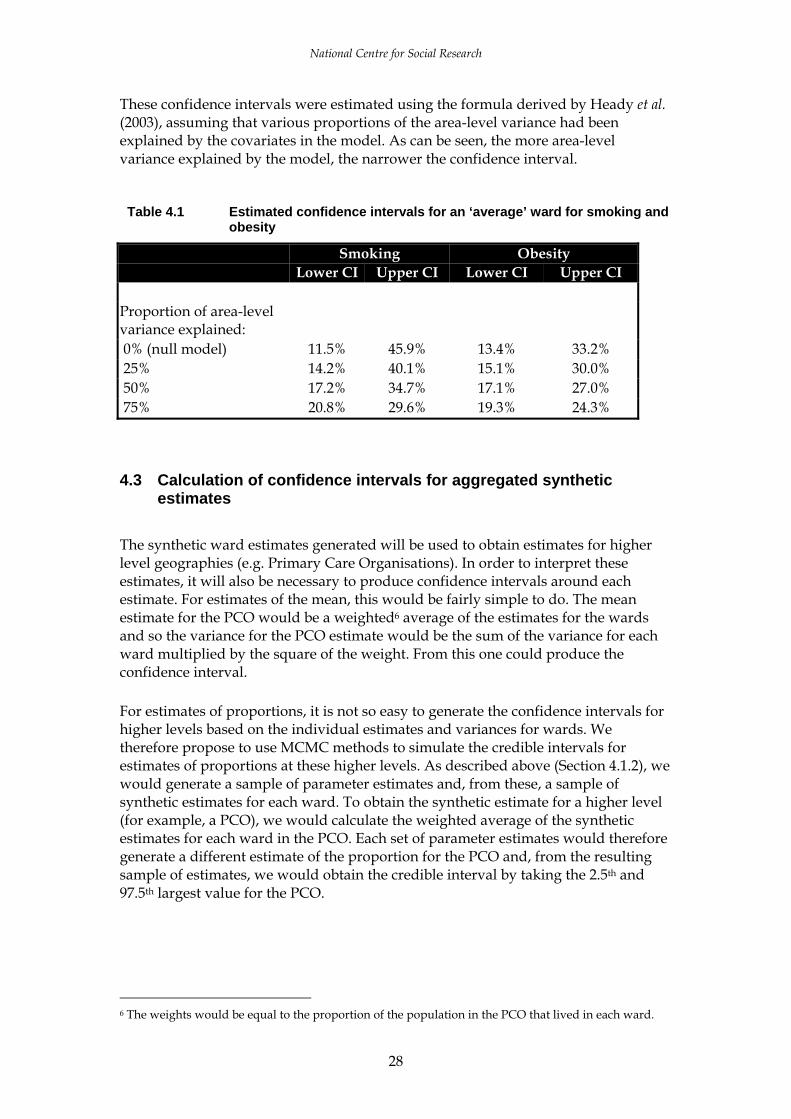
4.2 Indicative confidence intervals for wardsTable 4.1 shows the confidence intervals for smoking and obesity prevalence for an‘average’ ward that could be expected to be obtained from the synthetic estimation.


28

These confidence intervals were estimated using the formula derived by Heady et al.(2003), assuming that various proportions of the area-level variance had beenexplained by the covariates in the model. As can be seen, the more area-levelvariance explained by the model, the narrower the confidence interval.

Table 4.1 Estimated confidence intervals for an ‘average’ ward for smoking andobesity

Smoking ObesityLower CI Upper CI Lower CI Upper CI

Proportion of area-levelvariance explained: 0% (null model) 11.5% 45.9% 13.4% 33.2% 25% 14.2% 40.1% 15.1% 30.0% 50% 17.2% 34.7% 17.1% 27.0% 75% 20.8% 29.6% 19.3% 24.3%

4.3 Calculation of confidence intervals for aggregated syntheticestimates

The synthetic ward estimates generated will be used to obtain estimates for higherlevel geographies (e.g. Primary Care Organisations). In order to interpret theseestimates, it will also be necessary to produce confidence intervals around eachestimate. For estimates of the mean, this would be fairly simple to do. The meanestimate for the PCO would be a weighted6 average of the estimates for the wardsand so the variance for the PCO estimate would be the sum of the variance for eachward multiplied by the square of the weight. From this one could produce theconfidence interval.

For estimates of proportions, it is not so easy to generate the confidence intervals forhigher levels based on the individual estimates and variances for wards. Wetherefore propose to use MCMC methods to simulate the credible intervals forestimates of proportions at these higher levels. As described above (Section 4.1.2), wewould generate a sample of parameter estimates and, from these, a sample ofsynthetic estimates for each ward. To obtain the synthetic estimate for a higher level(for example, a PCO), we would calculate the weighted average of the syntheticestimates for each ward in the PCO. Each set of parameter estimates would thereforegenerate a different estimate of the proportion for the PCO and, from the resultingsample of estimates, we would obtain the credible interval by taking the 2.5th and97.5th largest value for the PCO.

6 The weights would be equal to the proportion of the population in the PCO that lived in each ward.


29

5 TESTING THE SOFTWARE

We have two options for the statistical packages that we can use to fit the multilevelmodels and subsequently produce the synthetic estimates: MLwiN and Stata. Thesepackages fit the multilevel logistic regression models using different methods7,although the parameter estimates produced are very similar.

Using Stata does offer several advantages over MLwiN for fitting the requiredmodels and producing the synthetic estimates for this project. These include:

• being generally much more user-friendly;• having a simple-to-use statistical test of adding one or more additional covariates

to the model (testparm);• it being much easier to produce the standard errors for the synthetic estimates for

synthetic estimates based on area-only models; • being more stable (MLwiN does tend to crash).

However, we will need to use MLwiN to run the MCMC procedure in order toobtain the credible/confidence intervals, as Stata does not perform MCMC methods.

Given the above, our plan is to use Stata to build the models – first by performing astepwise logistic regression, assuming the sample to be unclustered and with a p- value of 0.10, and then obtaining the optimal clustered model using the xtlogitcommand. Having obtained the optimal model in Stata, we would then fit, andcheck, the same model in MLwiN. Having made any necessary adjustments to themodel, we would obtain the point estimates from the standard MLwiN procedure(IGLS/RIGLS) and then run the MCMC procedure in order to obtain a sample ofparameter estimates in order to estimate the credible intervals.

7 MLWin fits the linear multilevel model using either Iterative Generalised Least Squares (IGLS) orrestricted IGLS (RIGLS) algorithm. Models for binary outcome are fitted with a logistic (or probit) linkfunction and binomial error term using a first- or second-order Taylor series expansion by iterating withthe standard IGLS or RIGLS algorithm (Goldstein;, 1995). The higher level random effect terms caneither be modelled as being in side the link function, the penalized quasi-likelihood (PQL) model, oroutside the link function, the marginal quasi-likelihood (MQL) model. Wherever possible, we wouldwant to fit second-order PQL models.

The corresponding function in Stata is called xtlogit (cross-sectional time series logistic regression). Thisfunction fits a logistic regression model with a level-two random effect (in this example representing thearea-level variance) using M-point Gauss-Hermite quadrature (StataCorp, 2003). If more complexmultilevel models were required, then these can be fitted using the gllamm command, which allowsadditional random effects to be included in the model (Rabe-Hesketh et al., 2002). For our purposes,this can be considered to be a more flexible version of the xtlogit command.


30

6 RECOMMENDATIONS FOR STAGE 2

6.1 Choice of estimation area Previous work done by the research team has shown that fairly robust directestimates from the HSfE can be calculated for large areas such as the 28 StrategicHealth Authorities and nine Government Office Regions (Scholes et al., 2004).Choices for synthetic estimation at lower level geographical areas include (in order ofdescending size) PCOs, LADs, wards, Super Output Areas and Output Areas (OAs).

In principle, synthetic estimation at the smallest possible area would be the optimalchoice as it offers at least two important advantages. First, from the users perspectivemore finely-defined estimates locate precisely the areas for targeted intervention.Second, they offer more flexibility of aggregation to respond to changes in higher-level geographies over time. One of the limitations of analysis at small areas such asSOAs/OAs is that the covariate dataset available at these levels will be restricted tothe more limited cross-tabulations available from the Census due to the applicationof disclosure control thresholds (i.e. CAS and ST tables). Other than the ID2004, thereare no administrative datasets available (e.g. benefit claimant rates, Hospital EpisodeStatistics, mortality rates) at these small levels.

However, the main reason for not opting for analysis at the SOA/OA levels arestatistical constraints imposed by the survey design. As mentioned previously, theHSfE is a clustered sample at postcode sector level. The population size of postcodesectors is similar to that of wards (about 5,000). Heady et al. (2003) have shown that,because of the similarity between the two, confidence intervals based on the variancebetween postcode sectors (rather than the variance between wards per se) givesreasonably accurate results. The same would not apply for confidence intervalsaround OA synthetic estimates.

This is not to suggest that OA estimates could not be produced - synthetic estimatescould be generated by modelling using OA-level covariates. However, it would notbe possible to estimate the OA-level variance from this model (as there would bevery few cases in each OA) and hence we would not be able to produce confidenceintervals for the estimates. In addition, our ability to validate the estimates at thislevel would be very limited.

For these reasons we suggest that wards should be the estimation level for thisproject. Wards also offer a number of other advantages such as:

- a wider range of available (non-census) covariate information than at smallerarea levels;

- local users are familiar with ward locations in their areas;- is possible to compare lifestyle estimates against other data available at ward

level such as NHS activity (HES data) and mortality; and- previous experience (e.g. by ONS) indicates that ward estimates are fairly

robust.


31

The main disadvantage of choosing wards as our estimation level is that wardboundaries change over time. This affects the relevance of estimates for the wardsaffected, and occasionally when such changes also impact upon the higher levelboundaries within which wards nest, aggregated estimates at the higher levels willalso no longer be valid.

6.2 Which models to test?We believe that the only two modelling approaches that could produce reasonablesynthetic estimates are the two multi-level model methods, namely the model withcovariates at the area level only, and the model with covatiates measured at both thearea and the individual level. The simple model (i.e. the model with individualcovariates only) can, we think, be dismissed on the grounds that other researchsuggests that there are genuine area impacts on health, so excluding them from themodel would inevitably give biased estimates.

Nevertheless, we will construct estimates where simple area effects are taken intoaccount by generating separate HSfE prevalence estimates within ID2004 quintiles orby area typology (ONS cluster). If these estimates are close to the synthetic estimatesgenerated using other means we will consider whether there would be benefits inusing them on the grounds that the estimates are simpler to understand and toreplicate.

6.3 Which health measures?The health measures to be tested at Stage 2 are those that we consider we will bemost likely to be able to generate reasonable synthetic estimates for (on the groundsthat, if we can’t achieve reasonable estimates for these, then we have little chance ofgetting reasonable estimates for other outcomes).

The criteria for choosing the estimates to take forward to Stage 2 are:• they should demonstrate a fairly large between-area variance;• they should be known to be correlated with the variables that will be used in the

models (i.e. age, sex, social class, area deprivation etc.);• should provide a geographical spread of areas.

Our suggestions for the outcomes to include in Stage 2 (with reason for selection inparenthesis) are:• prevalence of obesity among adults (objective outcome with low measurement

error);• prevalence of current cigarette smoking among adults (availability of good

covariate information and possible source for external validation); and• proportion of children aged 5-15 consuming five portions of fruit and vegetable a

day (estimates for a smaller sub-group of the sample and pooled over feweryears).


32

These three outcomes capture a range of lifestyle outcomes of policy interest and, ontechnical criteria, are diverse enough to form an assessment of what types ofoutcomes are suited to synthetic estimation.

6.4 Proposed approach to model validation The models tested at Stage 2 will be subjected to both internal and external validationchecks wherever possible.

The internal validation checks will include a range of formal ‘goodness of fit’measures. The ONS have outlined a number of strategies relevant to testing thosemodels underlying the synthetic estimates they have produced (Brown et al., 2001;Heady et al., 2003), many of which involve testing aggregates of synthetic estimatesfor larger geographical areas (such as the LADs) against sample-based estimates forthese geographical areas (assuming the sample size per area is large enough).

Put briefly internal model diagnostics will include:

for larger areas of geography such as LADs and PCOs plots of the model-basedsynthetic estimates (aggregated up to these larger areas) against direct surveyestimates. These plots give an indication of possible bias which Brown et al.(2001) describe as a ‘bias diagnostic’;

a ‘coverage diagnostic’ can be used to measure the overlap between the 95%confidence intervals for the two sets of estimates described above. A note ofcaution however in over reliance on confidence intervals. The danger lies in thecase where the underlying model does not provide a good approximation toreality. In the case of model misspecification, an assessment of model errorbased on the variance alone will be highly misleading; and

random split samples. This would involve randomly splitting the HSfE sampleinto two and re-fitting the models for each sub-sample. If our original modelwas stable, then we would expect the models to be fairly similar for both sub-samples.

For external validation we propose a less formal approach which involves, wherepossible, comparing synthetic estimates at ward level with direct estimates at wardlevel from other surveys. The main candidates here are local HSfE boosts – Camden& Islington, and Manchester if available in time – and other survey sources such asthe MRC One Million Women study (if we can secure access to the data).

Finally, the set of synthetic estimates that appear to be ‘best’ on these validationchecks will, we hope, be checked for ‘face validity’ by a panel of PCOs (see Section6.5). We will seek advise from the project management committees (particularly theUser and Technical Group members) for suggestions on selecting and gainingcooperation from selected PCOs across the country.


33

6.5 User engagementThe project has incorporated a programme of active user consultation andinvolvement throughout the study, working closely with the User Group and thewider user community. Immediately prior to the project being commissioned, usersand stakeholders in policy, local agencies, academia and the wider researchcommunity were invited to participate in the first user consultation meeting.Information needs and priorities were discussed and these formed the backdrop tothe sorts of issues that have been considered in this scoping study in terms oftechnical production and the relevance of estimates to users.

In Stages 2 and 3 of the study we will seek user involvement in three key areas:

• Result validation: comparing synthetic estimates with direct estimates fromlocal surveysUsers will be contacted by the User Group to help identify recent local surveyswhich include information about health behaviours. Analysis to compare thesynthetic estimates with available sources of local data will be central toestablishing the plausibility of the model-based estimates.

• ‘Blind testing’: comparing ranks of wards in local areas against localknowledge. Participation of groups of local users (or expert panels comprising localstakeholders) will be sought to verify whether the synthetic estimates correspondwith local knowledge and experience of ‘best/worst’ wards in their localities.Blind testing would involve users shading in a blank map of their area, indicatingwards that they think will score high, intermediate or low with respect to thedistribution of an outcome (say, prevalence of smoking) within their area.Representatives from PCOs and LADs will be approached to volunteer for thisexercise. Ideally, we'd like to use this form of face validity test for as wide a mixof different types of areas as possible (inner city, urban, rural, north/south, highethnic minority concentrations, level of deprivation etc).

• Expert input into production of user guide.We will ask members of the UG and the wider user community to providescenarios or examples of how they envisage using the synthetic estimates (e.g.comparing wards within PCOs or combining estimates with other data foranalysis). Responses to each scenario, indicating how and for what types ofanalyses synthetic estimates could (or could not) be used, with worked examplesand guidance on how to interpret the results will be included in the user guide.

In addition to the above key areas, in Stage 3 (implementation stage) user input willbe encouraged via consultations to feed into decisions about the selection of the final(five) outcomes and suggestions for forms of dissemination best suited to reach adispersed network of users.


34

REFERENCES

Ambler R, Caplan D, Chambers R, Kovacevic M and Wang S (2001) ‘Combiningunemployment benefits data and LFS data to estimate ILO unemployment for smallareas: An application of a modified Fay-Herriot method’, Proceedings of theInternational Association of Survey Statisticians, Meeting of the International StatisticalInstitute, Seoul, August 2001.

Brown G, Chambers R, Heady P and Heasman D (2001) ‘Evaluation of small areaestimation methods – an application to the unemployment estimates from the UKLFS’ Statistics Canada Symposium Ottawa, October 2001.

Charlton J (1998) ‘Use of the Census Sample of Anonymised Records (SARs) andsurvey data in combination to obtain estimates at local authority level.’ Env & PlaningA, vol 30, pp 775-784.

Chesterman J, Judge K, Bauld L and Ferguson J (no date) ‘How effective are smokingcessation services in reaching smokers in disadvantaged areas in England?’, Reportto Department of Health.

Cox D and Hinkley D (1974) Theoretical Statistics. London: Chapman and Hall.

Flowers J (2003) ‘Development of a indicator of needs-adjusted statin precribing atPCO level’ (unpublished report, Eastern Region PHO).

Gibson A, Asthana S (2001) ‘Resource allocation methodologies for the preventionand treatment of specific diseases - a critical review’. Discussion paper to ACRA(2001) 08, NHSE.

Goldstein H (2003) Multilevel statistical models (New York: Halstead Press).

Goldstein H (1995) Multilevel Statistical Models, John Wiley & Sons, New York.

Gilks W, Richardson S and Spiegelhalter D (1996) Markov Chain Monte Carlo inPractice. London: Chapman and Hall.

Heady P, Clarke P and others (2003) Model-based small area estimation series No 2(Small Area Estimation Project Report: Office for National Statistics).

Heady P, Clarke P, Brown G, D’Amore A and Mitchell B (2000) ‘Small area estimatesderived from surveys: ONS central research and development programme’ Statisticsin Transition (4: 635-648).

Levy P (1979) ‘Small Area Estimation – synthetic and other procedures, 1968-1978’ inNational Center for Drug Abuse Synthetic Estimates for Small Areas (ResearchMonograph 24: Washington D.C).

Macintyre S, Ellaway A and Cummins S (2002) ‘Place effects on health: how can weconceptualise, operationalise and measure them?’, Soc Sci Med. 2002 Jul;55(1):125-39.

Moura F and Holt D (1999) ‘Small area estimation using multilevel models’ SurveyMethodology (25: 73-80).

Rabe-Hesketh S, Skrondal A and Pickles A (2002). Reliable estimation of generalizedlinear mixed models using adaptive quadrature. The Stata Journal 2, 1-21.


35

Saei A and Chambers R (2003) ‘Small area estimation: A review of methods based onthe application of mixed models’ S3RI Methodology Working Paper M03/16.

Schaible W (1996) (ed) Indirect Estimators in U.S. Federal Programs (New York:Springer).

Scholes S, Prescott A and Bajekal M (2004) Health and Lifestyle Indicators for StrategicHealth Authorities, 1994-2002 (Department of Health) available at www.dh.gov.uk/PublicationsAndStatistics/PublishedSurvey/ HealthSurveyforEngland/HealthSurveyResults

StataCorp (2003) Stata Statistical Software: Release 8.0. College Station, TX: StataCorporation.

Skinner C (1993) The use of synthetic estimation techniques to produce small areaestimates OPCS New Methodology Series NM18. (London: Office for PopulationCensuses and Surveys).

Twigg L, Moon G and Jones K (2000) ‘Predicting small-area health-related behaviour:a comparison of smoking and drinking indicators’ Social Science and Medicine (50:1109-1120).

Twigg L, Moon G (2002) ‘Predicting small area health-related behaviour: acomparison of multilevel synthetic estimation and local survey data’, Social Scienceand Medicine 54(6):931-7.

Synthetic estimation of healthy lifestyles indicators...

Documents

Transcript of Synthetic estimation of healthy lifestyles indicators...