1

Author: Joline Cornelissen Supervisor: M.G. Contreras, PhD. Second reader: K. Burzynska, PhD. Submission date: October 19, 2016

SYNDICATED LENDING AND RELATIONS

2

Author: Joline Cornelissen

Student number: 4139356

University: Radboud University Nijmegen

Faculty: Nijmegen School of Management

Department: Economics and Business Economics

Supervisor: M.G. Contreras, PhD.

Second reader: K. Burzynska, PhD.

Submission date: October 19, 2016

Master’s thesis Economics – track Financial Economics

Syndicated lending and

relations Syndication, prior partnerships and locational proximity in Project Finance

lending

3

Acknowledgements

This master’s thesis is the result of several months of study and research. By finishing this

master’s thesis I completed the master Financial Economics at the Radboud University

Nijmegen. Herewith I would like to thank the people who supported me during this research

project. First of all my supervisor M.G. (Martha Gabriela) Contreras, PhD. for her enthusiasm

on the subject and invaluable expertise, advice, feedback and constructive criticism. In addition,

I would like to thank my family and friends for their support and words of encouragement

during the writing process.

Nijmegen, October 2016

Joline Cornelissen

4

Abstract

In the face of the evolving global corporate loan market in which banks are prone to syndicate

to raise loans, syndicate formation is a relevant question. As being an important source of

capital, an understanding of how this market operates is worth acquiring. Also, gaining

knowledge on syndicate formation and the important relationships therein is important. This

master’s thesis contributes to the syndicated loans literature by providing evidence regarding

the nature of ongoing relations between syndicate members, more specifically, the exclusive

relationships between lead arranger(s) and borrowers are analysed. Using banks in the

syndicated lending market, this master’s thesis discusses the likelihood of lending, after

previous lending and other kinds of relations.

This master’s thesis examines the relationships between borrowers and lead arranger(s)

and its influence on loan syndicate formation. Based on a cross-section of 351 loan syndicates

involving 118 lead arrangers and 181 borrowers during the period of 1997–2014, this study

reports three main findings. First, the likelihood of syndicate formation is positively, but not

significantly, related to the reputation of the borrower, shown in the number of previous

syndicate partnerships. It could not be confirmed that within a firm's set of past partners, the

higher the number of previous ties or prior partnerships a borrower has had, the more likely it

is that a syndicate lending relationship will be formed between a bank or lead arranger and that

borrower. Second, when focusing on the relation between the borrower and the lead arranger,

their home country could be of importance in syndicate decisions. It is found that if syndicate

members, lead arranger(s) and borrowers, have their headquarters in the same location or

country, the more likely a loan syndicate is formed between those parties. Third, it could be the

case that the effect of a prior partnership on syndicate formation depends on the headquarter

countries of both the lead arranger and the borrower; if they are similar or not. However, no

significant results were found for this interaction effect.

With these results, this master’s thesis shows that relations (as in locational proximity)

lead to strong connections between lending and borrowing syndicate partners, leading to a

higher likelihood of syndicate formation.

Key words: project finance lending, syndicated (project finance) loan market, syndicated

lending, lead arrangers, borrowers, previous relationships, locational or geographical

proximity.

5

Table of Contents

Acknowledgements ................................................................................................................... 3

Abstract ..................................................................................................................................... 4

Chapter 1 Introduction ............................................................................................................ 7

1.1 Motivation and research ....................................................................................................... 7

1.2 Scientific relevance and theoretical contribution ................................................................. 9

1.3 Practical relevance and managerial implications .............................................................. 10

1.4 Structure ............................................................................................................................. 10

Chapter 2 Literature Review and Hypotheses .................................................................... 12

2.1 What is a 'syndicate'? ......................................................................................................... 12

2.2 Why do banks syndicate? – benefits and risks ................................................................... 14

2.3 Relations and collaboration within loan syndicates ........................................................... 16

2.4 Prior partnerships in syndicated lending ............................................................................ 17

2.5 Hypotheses ........................................................................................................................ 18

Chapter 3 Data and Methodology ......................................................................................... 20

3.1 Research methodology ....................................................................................................... 20

3.2 Data and sample ................................................................................................................. 20

3.3 Measures ............................................................................................................................. 22

3.3.1 Dependent variable .................................................................................................. 22

3.3.2 Independent variables .............................................................................................. 23

3.3.3 Control variables ...................................................................................................... 25

3.4 Research method and the choice of estimation strategy .................................................... 27

Chapter 4 Empirical Results ................................................................................................. 30

4.1 Descriptive statistics and correlation matrix ...................................................................... 30

4.2 Assumptions ....................................................................................................................... 34

4.3 Results ................................................................................................................................ 36

4.3.1 Control variables ...................................................................................................... 37

4.3.2 Independent variables .............................................................................................. 38

6

4.3.3 Interaction effect ...................................................................................................... 38

4.4 Robustness checks .............................................................................................................. 39

Chapter 5 Conclusion and Discussion .................................................................................. 44

5.1 Conclusion .......................................................................................................................... 44

5.2 Limitations and future research possibilities ...................................................................... 46

Bibliography ........................................................................................................................... 50

Appendices .............................................................................................................................. 57

Appendix A – Variance Inflation Factor (VIF) ........................................................................ 57

Appendix B – Fit statistic ......................................................................................................... 58

Appendix C – Logistic regression ............................................................................................ 60

7

Chapter 1 Introduction

1.1 Motivation and research

The corporate loan market has evolved over the past twenty years: the number and types of

loans issued on a yearly basis have changed, but also the composition of the banks issuing them.

It is observed that the corporate loan market has grown in recent years in terms of size and

activity levels and is now a major source of funding for corporate organizations and

governments (Muzvidziwa, 2012). According to Bos, Contreras and Kleimeier (2013, p. 1),

“the ratio of loans arranged by multiple lead arrangers rose from just 13% to more than 80%”,

between 1990 and 2010. Panyagometh and Roberts (2010) even state that syndicated loans

currently represent the largest source of financing globally.

In the face of such an evolving corporate loan market in which banks are prone to

syndicate to raise loans, syndicate formation is a relevant question. Increasingly, the topic of

syndicated lending has attracted the attention of practitioners, policy-makers and, more

recently, academic researchers. The international market for syndicated credits or loans – loans

where several banks form a group to lend to a borrower – emerged as a sovereign business in

the 1970s and subsequently became a source of funding widely relied upon by corporate

borrowers (Altunbas, Gadanecz & Kara, 2006). It can be stated that syndicated loans are a large

and an increasingly important source of global corporate finance, exceeding the total annual

issuance volume of equity and bond markets (Bosch & Steffen, 2011). As an example, in the

U.S. alone, the market for syndicated loans has experienced strong growth, going from $137

million in 1987 to over $2.2 trillion in 2007, the year the syndicate market reached its peak

(Sufi, 2007; Bord and Santos, 2012). The syndicated loan market is one of the most important

sources of financing for large and medium-sized companies based on global transactions,

totalling three trillion dollars (Champagne and Kryzanowski, 2007). Privately held, high yield,

and investment grade firms all utilize this financial product.

During the past four/five decades, an important new method of financing large-scale,

high-risk domestic and international business ventures has emerged. This master’s thesis

researches this specific type of bank lending called project finance: a form of long-term

financing primarily used for infrastructure and development projects (Kleimeier and

Megginson, 2000). The technology called project finance, is usually defined as “limited or non-

recourse financing of a newly to be developed project through the establishment of a vehicle

company (separate incorporation)” (Kleimeier & Megginson, 2000, p. 76). Project loans are

8

made by commercial banks, with each lender agreeing that loans will be repaid only from the

revenues generated by the successful, completed project itself. “Loans normally contain loan

covenants or agreements between the lender and the borrower about what the borrower should

or should not do, such as providing regular reports and adequate insurance” (Somo, 2005, p. 1).

Larger, more risky projects often require syndicated loans. These loans are provided by a group

of financial institutions called a bank consortium or a syndicate (Somo, 2005).

As stated above, the market for syndicated loans has grown tremendously and is now a major

source of funding for corporate organizations. As being an important source of capital, an

understanding of how this market operates is worth acquiring, more specifically, further

knowledge on syndicate formation and the important relationships therein is worth acquiring.

In general, previous research on syndicated loans is limited when compared to research on

public equity and debt underwriting markets or venture capital (Li & Rowley, 2002). Most

papers on syndicated lending have analysed and evaluated syndicate structure (Sufi, 2007).

Central to syndicated loans are the unique relationships that exist between the

borrower(s), the lead arranger(s) and the participant lenders. An analysis of these relationships

and how these relationships affect loan syndications is critical (Muzvidziwa, 2012).

Furthermore, while most inter-bank relationships are not readily observable, loan syndicates

represent visible indications of bank interactions that can be studied. “The expanding literature

on syndicated loans ranges from syndicate composition to agency problems, however, little is

known about the underlying relationships behind this activity” (Champagne and Kryzanowski,

2007, p. 3146). So, despite the importance of syndicated loans, research on the role and working

of such loans in corporate finance is limited (Sufi, 2007).

Another central question involves why firms rely on their networks of past relationships

to form syndicated loan alliances. In a market where information asymmetries dominate, such

as in the syndicated loan market, a firm’s best strategy to obtain a loan or to borrow money is

often to borrow from a bank or multiple banks with whom they have previously collaborated

(Farinha & Santos, 2002). Thereby pooling resources and funds from different banks. However,

collaborating with new partners, as opposed to previous partners, could also be an option

(Contreras, 2016). But, past studies have consistently shown that firms show a propensity to

ally again with their past partners when forming alliances (Gulati, 1995; Gulati & Gargiulo,

1999; Uzzi, 1997). This behaviour has been associated with a need to have knowledge of

potential partners' capabilities and reliability (Li & Rowley, 2002). However, research on such

9

prior partnerships, and other relations, in relation to syndicate formation or syndicated loan

alliances is limited.

Given these deficiencies, the purpose of this master’s thesis is twofold. The first is to

explore the syndicated loan literature regarding the nature of ongoing relationships among

syndicate members. The second is to explore the influence or effect of relations or partnerships

between syndicate members, lead arranger banks or lenders and firms or borrowers, on the

formation of a loan syndicate. This results in the following research question:

‘What is the influence of relations between lending and borrowing syndicate partners on the

likelihood of syndicate formation?’

1.2 Scientific relevance and theoretical contribution

This paper contributes to the syndicated loans literature by providing evidence regarding the

nature of ongoing relations between syndicate members: lead arrangers and borrowers. The

evidence presented herein differs from and, in some ways, improves on a somewhat similar case

made by Sufi (2007) who found that (previous) relationships between syndicate members do

affect future alliances. However, Sufi (2007) has studied relationships among banks and this

master’s thesis studies relationships between different types of syndicate members: borrowers

and banks or lead arrangers.

Furthermore, previous papers have focused predominantly on the relationship of the

lead arranger with participants, such as Champagne and Kryzanowski (2007), Panyagometh &

Roberts (2010), Ivashina (2009) and Li, Eden, Hitt & Ireland (2008). This master’s thesis

focuses on the exclusive relationship between lead arrangers and borrowers since this

relationship comes before the future relationship between the lead arranger and participant

lenders. This because syndicated loan deals are characterized by the existence of a lead arranger

who establishes a relationship with the borrowing firm and after that the lead arranger negotiates

terms of the contract and organizes a syndicate of participant lenders who each fund part of the

loan (Ball, Bushman & Vasvari, 2008, p. 248). Furthermore, it is found that previous lead

arranger–participant relationships are much less important than previous relationships between

a borrowing firm and (participant) lender(s) (Sufi, 2007, p. 632).

10

1.3 Practical relevance and managerial implications

This thesis has several important implications for alliance or loan management. First of all,

instead of solely focusing on current information or knowledge of a potential lending or banking

partner, in addition managers should consider focusing on the knowledge that prior relations or

interactions with that partner possess. Another implication for alliance management is the

decision of which managers will participate in the syndicate collaboration. Since prior

partnerships between syndicate members (firm and banks) are important, managers that were

involved in such a prior loan syndicate could be of great importance for future syndicate loan

formations due to their experience with forming a lending agreement and due to increased trust

and partner knowledge. Both implications are related to the advantages of forming lending

relationships with prior partners. One advantage is that syndicated loan alliance experience

(entering into repeated lending relationships) can generate trust between partners. More

interactions between partners or syndicate members over time leads to higher trust and therefore

to larger loan contracts in monetary terms, as stated by Gulati (1995). This because trust can

reduce transaction costs and uncertainties (Barney & Hansen, 1994). According to Baum,

Rowley, Shipilov and Chuang (2005), prior partnerships allow each partner to learn about the

core competencies, operating routines, managerial practices, priorities, and reliability of the

other. Such stable relationships lead to a reduction of uncertainty surrounding transactions.

Next, another implication could be that concerns about search costs can prevent firms from

looking beyond their previous relationships. When this happens, firms become ‘locked’ into

established relationships, as found by Ellis (2000). As is found in this master’s thesis that

locational proximity influences syndicate formation, managers should not solely focus on prior

partnerships, but also take other partners into account that are in proximity, to prevent becoming

‘locked in’.

1.4 Structure

The remainder of this master’s thesis will be structured as follows. First, chapter 2 describes

existing literature and research related to this master’s thesis: literature on the syndicated loan

market, syndicated lending, project finance and reasons why lending partnerships are formed is

discussed. The literature discussed in this chapter forms the theoretical background or

framework for the hypotheses that are presented in the end of the chapter. Chapter 3 presents

the data and sample, summary statistics, and elaborates on the methods that are used in order to

determine the quantitative value of the dependent, independent and control variables. In chapter

11

4, a descriptive analysis provides a summary of the basis features of all variables which is used

in order to motivate the use of the estimation strategy. Next to that, chapter 4 presents the

empirical findings of the research and describes the additional tests which are applied in order

to check robustness and to account for outliers and multicollinearity. In chapter 5, the last

chapter of this thesis, the empirical findings are discussed in combination with previous

literature, in addition to the main limitations of the research setting and the implications for

practice. Finally, based on the results of this thesis, in chapter 5 possible suggestions and

recommendations for future research are discussed.

12

Chapter 2 Literature Review and Hypotheses

This chapter discusses the theoretical background of the research based on existing literature

and gives a state of the art literature overview on the different concepts surrounding syndicated

lending and relations. In the first part of this chapter, (loan) syndication is discussed as a lending

relationship between lead arrangers, participant lenders and borrowers. The second section

discusses the reasons for loan syndication, followed by a documentation of relations and

collaboration within loan syndicates in the third part. In the fourth section, the concept of prior

partnerships in syndicated lending is introduced and theoretically linked to the forming of loan

syndicates, which leads to the hypotheses that are empirically tested later in this thesis.

2.1 What is a 'syndicate'?

To start at the beginning, what exactly is a syndicate? A syndicate is a professional financial

services group formed for the purpose of handling large transactions, thereby handling that

transaction as a group instead of individually. Syndication allows companies to pool their

resources and share or spread (insurance) risks. There are several different types of syndicates,

including underwriting syndicates, insurance syndicates and banking syndicates, which this

thesis writes about. These are syndicates (or a collection) of a group of banks that work together

to issue new stock to the public or to jointly extend a loan to a specific borrower (Taylor &

Sansone, 2006).

As stated in the introduction, due to their large scale, project finance loans require large

amounts of capital. As a consequence, project finance loans are often syndicated. Loan

syndication refers to the joint issuance of loans by multiple banks (lenders). It is a process

involving a group of banks, at least two, which jointly make a loan, and thereby offer funds, to

a single or to multiple borrowing firms (Bos, Contreras & Kleimeier, 2013). Unlike a loan sale

to a third party, in which no direct contract exists between the borrower and the buyer,

“syndication involves a direct contract between each member bank and the borrower”. Lending

syndicates resemble pyramids with a few arranging banks (arrangers) at the top and many

providing banks (participants) at the bottom (Esty, 2003, p. 40).

Members, or banks part, of a (loan) syndicate fall into one of two groups, lead arrangers

and participant lenders. The distinction is important since the two groups vary on several

dimensions (Sufi, 2005). Explaining, loan syndication is a process whereby, at the moment of

loan issuance, a bank sells a share of the loan to other financial institutions. The lead (selling)

13

bank is appointed by the borrower to originate and syndicate the loan and is usually called the

‘arranger’ (Ivashina, 2005, p. 5). Lead arrangers (syndicate managers) are the most active banks

in the syndicate. Prior to closing a loan, the arranging (or mandated) banks are responsible for

meeting with the borrower, establishing and maintaining a relationship with the borrowing firm,

negotiating the loan contract terms, conditions and details, guaranteeing an amount for a price

range, assessing the credit quality, and they are responsible for monitoring, or conducting due

diligence on, the borrower (Sufi, 2007; Bos, Contreras & Kleimeier, 2016; Ivashina. 2005).

Once the key terms are in place, the arranging banks invite other banks to participate in the deal

(Esty, 2003). Besides this recruiting of passive participant banks to fund the loan, lead arrangers

also take responsibility for primary information collection, arranging documentation and

recruiting passive participant banks to fund the loan. By recruiting passive banks is meant that

the lead arranger turns to ‘participant’ lenders to fund part of the loan (Sufi, 2007). After

closing, the arranging banks monitor compliance with loan covenants, negotiate contingency

agreements as needed, and lead negotiations in default situations (Esty, 2003). Furthermore,

“during the life of the loan, lead arrangers monitor the borrower and share their findings with

the participant lenders” (Bos, Contreras & Kleimeier, 2013, p. 1-2). Lead arrangers share their

findings by drafting an information memorandum that contains detailed and confidential

information, such as information about the borrower’s credit worthiness and loan terms (Sufi,

2007). The potential participants have the opportunity to discuss the memorandum with the lead

arranger (Muzvidziwa, 2012). Also, the loan spread and the syndicate structure are

simultaneously determined in the process of syndication (Ivashina, 2005, p. 6). Lead arrangers

also “hold collateral, administer the loan and handle disbursements and repayments” (Bos,

Contreras & Kleimeier, 2013, p. 1-2).

Contrasting, participant lenders rarely directly negotiate with the borrowing firm. They

have a so called ‘arm’s-length’ relationship with the borrowing firm, through the lead arranger.

Participant lenders typically hold a smaller share of the loan than (any of) the lead arranger(s)

(Sufi, 2007). Participant banks consequently depend on the information collected by the lead

bank (Ivashina, 2009). As stated in the introduction, lead arrangers usually have strong lending

relations with the borrowers and receive significant upfront fees in exchange for arranging the

syndication deal and taking the underwriting risk (Altunbas et al., 2006). Participant banks

“typically earn only the interest rate margin, do not have origination capability, and are

interested in generating future business from the borrower such as treasury management or

advisory work” (Ball, Bushman & Vasvari, 2008, p. 254).

14

Concluding, typically the syndicate consists of lead arrangers and participant banks,

with lead arrangers being expected to actively monitor the borrower, and participants serving

to diversify loan risk without actively monitoring the lending relationship (Neuhann and Saidi,

2015). Because the arranging banks play a more prominent role than providing banks, leading

up to and after syndication, this master’s thesis focuses on the arranging or lead arranger

bank(s).

2.2 Why do banks syndicate? – benefits and risks

Loan syndication, where a group of banks (multiple arrangers) make a loan jointly to a single,

or to several, borrower(s), offers several benefits. Syndication allows banks to diversify their

loan portfolios and manage their risk, and to expand lending to broader geographic areas and

industries. Second, syndication allows banks that are constrained by their capital-asset or

liquidity ratios to participate in loans to larger borrowers, since syndication allows for flexibility

in determining the size of the lending share (Simons, 1993). By forming a syndicate, originating

banks diversify, share risk across the syndicate, information and (monitoring) skills, and can

more easily meet capital constraints (Simons, 1993; Ivashina and Scharfstein, 2010; Dennis and

Mullineaux, 2000). In a syndicate with lead arrangers having different knowledge, experience,

expertise, skills, competencies and specializations, lead arrangers can leverage each other’s

skills with the purpose of reducing information asymmetries in the loan arrangement process

(Tykvovà, 2007; Sufi, 2007; Champagne and Kryzanowski, 2007). Thus, an important

economic benefit from syndicating is the know-how transfer between partners resulting from

their ability to learn: multiple arrangers can combine their expertise (Tykvovà, 2007; Schure,

Scoones and Gu, 2005). But also, at the same time, various tasks and different kinds of expertise

can be allocated among lead arrangers to avoid double work, thereby reducing each arranger’s

effort costs. Syndication can also motivate participant banks to join, as they often have a lack

of experience in specific loan types or markets (Dennis and Mullineaux, 2000, Simons, 1993).

In short, it is found by Simons (1993), when examining the incentives to syndicate, that

diversification is the primary motive for syndication (Dennis and Mullineaux, 2000).

Despite these benefits, loan syndication could pose additional risks for the banking

system if the originating or lead banks withhold information about the borrower from

participating banks or mislead them into making loans that are riskier than they thought

(Simons, 1993). The most important costs associated with loan syndication result from agency

problems causing differences in the effort banks exert when arranging loans, in particular when

the differences in skills and competence levels among syndicate members are substantial (Lee

15

and Mullineaux, 2004; Tykvova, 2007). This could be the case for example “if a member of a

syndicate is much more competent (i.e., has better knowledge, more experience, etc.) than

another, the latter may free ride with the former exerting more effort in the syndication process”

(Bos, Contreras & Kleimeier, 2016, p. 6). A study by Simons (1993), which uses data on loan

syndications to test the importance of various factors that motivate the syndicate participants,

finds little evidence of opportunistic behaviour by the lead banks or arrangers in syndications.

This despite a significant number of ‘problems’ among the syndicated loans studied.

When looking at it from another side, banks may also syndicate with the purpose of

reducing information asymmetries with borrowers. A paper by Das and Nanda (1999) finds that

loans arranged by joint banks reduce information asymmetries, related with the borrower and

the syndicated loan. Lead arrangers are the only syndicate members that directly interact with

borrowers and therefore need to have information about for example their identity, lending

history, and risks that can be associated (Bos, Contreras & Kleimeier, 2013). According to

Dennis and Mullineaux (2000), loans are more likely to be syndicated by lead arrangers when:

the loan is large, the borrowing firm is public, and the lead arranger has a strong reputation.

They also find that, conditional on a loan being syndicated, a larger percentage of the loan is

syndicated when there is public information on the borrowing firm and when the lead arranging

bank has a strong reputation (trustworthy syndicate partner). Thus, loan syndications are more

likely when the information about the borrower becomes more transparent, through repeated

market transactions, when public information on the borrower is available and when the

reputation of the lead arranger is strong (Muzvidziwa, 2012). So, the likelihood of loan

syndication depends on the availability of information and knowledge, which both syndicate

parties (lead arrangers and borrowers) need from each other.

Concluding, loan syndication is more beneficial rather than risky, especially when there

is a higher need to reduce or mitigate informational asymmetries about for example the quality

of the borrowing firm, e.g. higher monitoring needs, and when knowledge and skill sharing

between lead arrangers is important (Bos, Contreras & Kleimeier, 2013, p. 2). According to

Bos, Contreras and Kleimeier (2013, p. 2), this kind of knowledge and effort sharing by banks,

when forming a loan syndicate (jointly arranging a loan), “is especially valuable when the loan

is complex and monitoring needs are higher”. This is the case for project finance loans since

the required expertise for such loans is specific and extensive. Therefore benefits of sharing

from forming a syndicate are high. So, information asymmetry problems can be existent,

however the benefits of syndication, such as knowledge and monitoring capital needs, outweigh

the problems.

16

2.3 Relations and collaboration within loan syndicates

Through time, collaboration among lead arrangers through syndicated loans, within the global

syndicated loan market, has contributed to the development of a dense and complex social

network of banks (Bos, Contreras & Kleimeier, 2013). Network connections across banks are

common, and have become increasingly prevalent over time. “The total number of lead

arrangers is large and the increasing rates at which banks syndicate, render a complex network

of banks consisting of lead arrangers that are linked to each other when they co-arrange a loan”

(Bos, Contreras & Kleimeier, 2013, p. 2). Thus, loan syndication increases bank

interconnectedness through co-lending relationships (Nirei, Sushko and Caballero, 2016).

Those connected banks “are more likely to partner together in loan syndicates” (Houston, Lee

and Suntheim, 2015, p. 4). There are thus extensive social networks that exists within the global

banking system. Champagne and Kryzanowski (2007) even highlight that the sustainability of

the global loan markets, especially loan syndications, relies on a complex network of ties

between financial institutions.

Besides social connections between banks or lead arrangers within loan syndicates,

other syndicate connections exist, between banks and borrowers for example. In a world with

asymmetric information flows, relationship lending may restore efficiency by establishing long-

term implicit contracts between borrowers and lenders. Lenders or banks thus develop close

relationships with borrowers or firms, over their time of lending (Berlin, 1996). “An established

relationship allows the lender to renegotiate contract terms at low cost, thereby decreasing

aggregate financing cost and reducing credit rationing. The financial relationship is effectively

a long term commitment in which lenders have an informational privilege vis-à vis both the

market and competing banks, by which they gain some degree of ex post bargaining power”

(Elsas & Krahnen, 2000, p. 3-4). It can be stated that both close proximity between banks

(lenders) and borrowers and the development of information-intensive relationships between

them, facilitate monitoring and screening. Furthermore, those tight relationships can overcome

problems of asymmetric information between the parties. So, network connections across banks

and firms (borrowers) can be beneficial.

Concluding, extensive ties or connections within the global syndicated loan market not

only lead to strong connections between lending partners and to more active business

partnerships and/or similar investments among connected banks (lenders) (Houston, Lee and

Suntheim, 2015), but also lead to strong connections (as in previous partnerships or proximity)

between lending and borrowing partners. This suggests that such ties generate valuable

17

information which translate into business connections and a higher likelihood of partnering

together in loan syndicates.

2.4 Prior partnerships in syndicated lending

As stated in the introduction, this thesis focuses on a specific type of bank lending: project

finance lending, for which often syndicates are formed. Firms that want to obtain lending can

collaborate in a syndicate with banks with whom they have previously collaborated, and thus

had a prior partnership with, or with new partner banks. Thereby, this thesis investigates the

impact of past syndicate alliance relationships on future alliances based. Consistently it is found

that firms favour past partners: once a firm has borrowed from a given bank, it has an incentive

to borrow from it again. This because this ‘past’ bank is “better positioned to enforce

compliance with the terms of the new loan because of the firm specific information it has

already learned” (Farinha & Santos, 2002, p. 124).

Literature on previous relationships among syndicate members finds that such

relationships are important in determining which lenders end up participating as syndicate

members. Previous relationships between the lead arranger and a potential participant lender

increases the probability that the potential participant becomes a syndicate member (Sufi,

2007). However, it is found that “previous lead arranger–participant relationships are much less

important (both in magnitude and statistical significance)” than previous relationships between

a borrowing firm and lender(s) (Sufi, 2007, p. 632). Therefore, this master’s thesis focuses on

relationships between borrowers and lenders (as syndicate members), instead of relations

between different kinds of lenders. Besides the fact that prior partnerships play an important

role in the likelihood of syndicate formation, Champagne and Kryzanowski (2007) also find

that the probability of joining a syndicate is positively related to the number of lenders in the

syndicate, the reputation of the borrower and whether the lead and the borrower are from the

same country. But, why do borrowers and lead arrangers mostly rely on their local networks of

past relationships when participating in a syndicate?

Research reveals that firms or borrowers follow a logic of reducing uncertainty and risk

in their exchanges or syndicate relations by engaging past partners in repeated ties (Gulati and

Gargiulo, 1999) rather than seeking for riskier and more uncertain nonlocal ties beyond local

clusters (Li and Rowley, 2002). Here, nonlocal ties can be characterized as new or non-prior

partnerships with lead arrangers. Podolny (1994) has found that the greater the market

uncertainty, the more that firms engage in relations with those with whom they have transacted

in the past (due to greatest knowledge). For the other important party in this master’s thesis, the

18

banks or lead arrangers it is found that “because banks potentially pay a high price for engaging

with ineffective partners, they should be particularly wary of unfamiliar nonlocal partners and

rely heavily on engaging past partners within their circle of embedded ties” (Baum, Rowley,

Shipilov and Chuang, 2005, p. 547). This because, among the key benefits ‘lost’ in nonlocal

syndicate ties are knowledge of partners' marketing abilities, reliability, and willingness to

collaborate (Baum, Rowley, Shipilov and Chuang, 2005, p. 547-548). Furthermore, imperfect

information about potential partners' capabilities, reliability, and motives creates considerable

risk and uncertainty in syndicate relationships (Baum, Rowley, Shipilov and Chuang, 2005, p.

536). So, when choosing from constrained ties, choosing past partners is most beneficial, for

both banks as firms. Thereby reducing risk and uncertainty in future relationships (Baum,

Rowley, Shipilov and Chuang, 2005).

2.5 Hypotheses

Within a firm's set of past partners (local network), the higher the number of previous ties or

prior partnerships that firm or borrower has had, the more likely it is that a syndicate is formed

between that borrower and a bank or lead arranger (Champagne and Kryzanowski, 2007). As

found by Champagne and Kryzanowski (2007): the likelihood of syndicate formation is

positively related to the reputation of the borrower, shown in the number of previous

partnerships. This leads to the first hypothesis:

‘If the number of previously established syndicate or lending relationship or prior partnerships

a borrower has had increases, the more likely a loan syndicate is formed between that borrower

and (any) lead arranger(s)’.

Furthermore, when focusing on the relation between the borrower and the lead arranger, their

home country could be of importance in syndicate decisions. As stated in the literature review,

Champagne and Kryzanowski (2007) find that the likelihood of joining a syndicate is positively

related to whether the lead and the borrower are from the same country. So, a lead arranger may

be more likely to give repeat business to a particular borrower due to its physical proximity.

This leads to the second hypothesis:

‘If syndicate members, lead arranger(s) and borrowers, have their headquarters in the same

location or country, the more likely a loan syndicate is formed between those parties’.

19

For both hypotheses it matters that extensive relations (as in previous partnerships or locational

proximity) lead to strong connections between lending and borrowing syndicate partners,

thereby influencing the likelihood of syndicate formation.

Next, it could also be the case that the effect of a prior partnership on lead arranger-borrower

funding or syndicate formation depends on the headquarter countries of both the lead arranger

and the borrower; if they are similar or not. This leads to the third hypothesis:

‘If syndicate members, lead arranger(s) and borrowers, are from the same country, the

influence of a prior partnership matters more, so the more likely a loan syndicate is formed

between those parties’.

20

Chapter 3 Data and Methodology

In this chapter, the research design is explained which constitutes the foundation for the

empirical analysis. First of all, the research methodology and the research setting will be

discussed. Argumentation for a quantitative research will be presented. Furthermore, the

methods that will be used for collecting data are elaborated. Next, the nature of the independent

and dependent variables is explained together with the measurements of these variables. Finally,

the control variables that are included in the research model are introduced.

3.1 Research methodology

According to Ahrens & Chapman (2006, p. 822), a research methodology can be defined as

“the general approach taken to the study of a research topic, which is independent from the

choice of methods” (Chapman, Hopwood & Shields, 2007). This master’s thesis attempts to

explore the influence or effect of relations between syndicate members, lead arranger banks or

lenders and firms or borrowers, on the formation of a loan syndicate, while providing additional

information with regard to the nature of the relation. In describing the relationship between

prior borrower partnerships, locational proximity and the likelihood of syndicate formation, a

quantitative research methodology is conducted. According to Creswell (2013, p. 18),

quantitative research makes use of “cause and effect thinking, reduction to specific variables

and hypotheses and questions, use of measurement and observation, and the test of theories”.

This master’s thesis does not try to understand surroundings, or a specific context, but it focuses

on reduction to specific variables. Furthermore, the concepts described in this master’s thesis

can, for the purpose of this research, be reduced to specific or measurable variables, so that

quantitative research is most suitable.

3.2 Data and sample

The Loan Pricing Corporation’s (LPC) DealScan database provides data on global corporate

loans; it is a database of loans to large firms (Bos, Contreras & Kleimeier, 2016). DealScan is

the world's number one source for comprehensive, reliable historical deal information on the

global loan markets. Furthermore, DealScan is the main data source for research in syndicated

lending. It contains information about syndicates and syndicate members (Dennis and

Mullineaux, 2000; Sufi, 2007; Champagne and Kryzanowski, 2007; Ivashina and Scharfstein,

2010; Godlewski, Sanditov, and Burger-Helmchen, 2012). The DealScan database by Thomson

21

Reuters Loan Pricing Corporation is used as the only source of data on global corporate loans

and on the syndicated loan market. “This database contains detailed historical information on

the entire population of global corporate loans, including syndicated loans, made to medium

and large sized U.S. and foreign firms” (Bos, 2016). Furthermore, it contains detailed

information on syndicated loan contract terms, lead arrangers, and participant lenders. The

primary sources of data for DealScan are “attachments on SEC filings, reports from loan

originators, and the financial press” (Sufi, 2007, p. 636). Besides the DealScan database, two

other data sources are used to find data on the country of the lead arranger: the database

Bankscope, with a check in ThompsonOne. Bankscope, or the world banking information

source, is a comprehensive, global database of banks' financial statements, ratings and rating

reports, stock data for listed banks, and other types of bank related information (Bureau van

Dijk, 2016). ThomsonOne contains financial data from annual reports, as time series over

multiple years, with a focus on listed corporations across the world (Radboud University

Library, 2016). The country of the borrower was found via the DealScan database, just as all of

the other data used in the research.

An international sample is generated of public and non-public lending institutions

participating in loan syndicates involving at least two financial institutions to extend a loan to

a single, or to multiple, borrower(s) between 1997 and 2014. The information in this dataset is

used for syndicate relationship representations of the syndicates formed between 1997 and

2014, since access to this data was given. Precise information about the lead arrangers involved

in each loan is needed, therefore, the loan observations that are used from DealScan contain

both, the lead arranger and number of arrangers, fields populated (Bos, 2016). The data provided

by DealScan allows investigation of the syndicate structure of these loans. Lead arrangers are

identified from DealScan’s ‘Lead Arrangers’ field, which is in line with Sufi (2007) (Bos,

Contreras & Kleimeier, 2016). When looking at the sources of the data, most of the borrowers

listed in the data products are publicly held companies, which are required to file with the

Securities and Exchange Commission (SEC) in Washington, D.C. Data from privately held

companies is available to a limited degree. If the company is private but has public debt

securities traded, the company must file. The remaining portion of the deals comes from direct

research from banks where LPC may initially obtain partial or unconfirmed information

(Kellogg School of Management, 2016).

The number of lead arrangers per loan is calculated by using the number of commas

plus one, in the Lead Arranger field when this one is non-empty. Following this methodology,

it is found that approximately 68% of the deals in the dataset have multiple lead arrangers. Thus,

22

the majority of bank loans are arranged by multiple lead arrangers. The loans that have more

than one lead arranger range between 2 and 7 lead arrangers per syndicate. The maximum

number of lead arrangers in a loan is found to be 23 in a loan issued in 2014. The number of

lenders per loan are validated by calculating the number of commas plus the number of colons,

in the AllLenders field when this one is non-empty. Following this methodology, it is found

that approximately 97% of the deals in the dataset have multiple lead arrangers: the majority of

bank loans are arranged by multiple lenders. The maximum number of lenders in a loan is found

to be 51 in a loan issued in 2011.

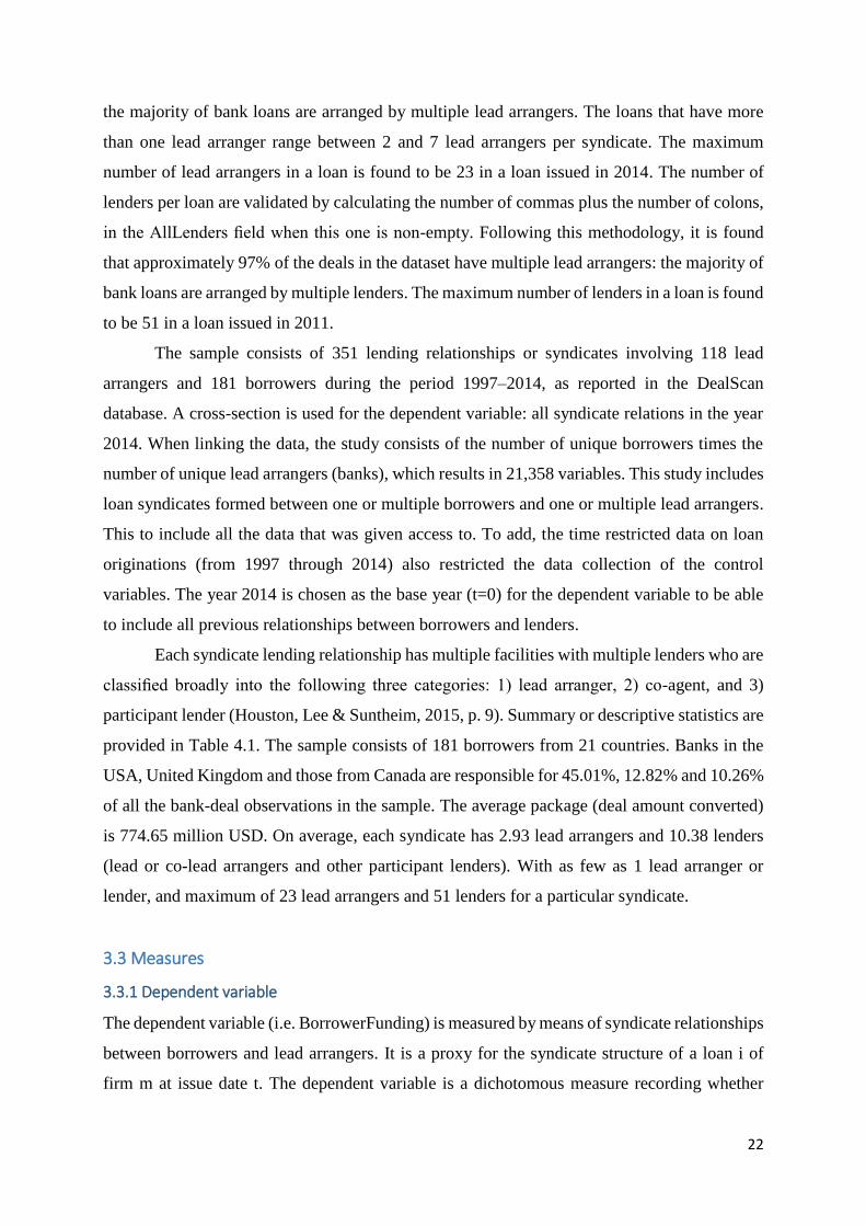
The sample consists of 351 lending relationships or syndicates involving 118 lead

arrangers and 181 borrowers during the period 1997–2014, as reported in the DealScan

database. A cross-section is used for the dependent variable: all syndicate relations in the year

2014. When linking the data, the study consists of the number of unique borrowers times the

number of unique lead arrangers (banks), which results in 21,358 variables. This study includes

loan syndicates formed between one or multiple borrowers and one or multiple lead arrangers.

This to include all the data that was given access to. To add, the time restricted data on loan

originations (from 1997 through 2014) also restricted the data collection of the control

variables. The year 2014 is chosen as the base year (t=0) for the dependent variable to be able

to include all previous relationships between borrowers and lenders.

Each syndicate lending relationship has multiple facilities with multiple lenders who are

classified broadly into the following three categories: 1) lead arranger, 2) co-agent, and 3)

participant lender (Houston, Lee & Suntheim, 2015, p. 9). Summary or descriptive statistics are

provided in Table 4.1. The sample consists of 181 borrowers from 21 countries. Banks in the

USA, United Kingdom and those from Canada are responsible for 45.01%, 12.82% and 10.26%

of all the bank-deal observations in the sample. The average package (deal amount converted)

is 774.65 million USD. On average, each syndicate has 2.93 lead arrangers and 10.38 lenders

(lead or co-lead arrangers and other participant lenders). With as few as 1 lead arranger or

lender, and maximum of 23 lead arrangers and 51 lenders for a particular syndicate.

3.3 Measures

3.3.1 Dependent variable

The dependent variable (i.e. BorrowerFunding) is measured by means of syndicate relationships

between borrowers and lead arrangers. It is a proxy for the syndicate structure of a loan i of

firm m at issue date t. The dependent variable is a dichotomous measure recording whether

23

borrower m entered into a syndicate relationship with bank or lead arranger j in the year 2014.

The dummy BorrowerFunding is equal to 1 if borrower m is a part of a syndicate with lead

arranger j in 2014 and is 0 otherwise. The year 2014 is chosen because it is the final year of the

accessible data, and therefore all the syndicate relationships in the years before 2014 represent

a prior relationship.

Another way of measuring the dependent variable BorrowerFunding is by recording the

funding dollar sum in the year 2014, between borrower m and lead arranger j. This way for

measuring the dependent variable is not included in the main analysis since the dichotomous

funding variable explained the most of the model; the proportion of the variance in the

dependent variable that is explained by the independent variables was the largest for funding as

a dichotomous measure. However, the dependent variable as the funding dollar sum in the year

2014 is included in the robustness checks section.

3.3.2 Independent variables

Several independent variables are included in this research and they all involve relations

between a lead arranger and the borrower. The financing options for borrowers include many

products with varying degrees of relationships. Syndicated loans fall between bank loans

(relationship lending) and public debt issues (transaction lending). In syndicated loans only the

lead arranger has a relationship with the borrower; the lead arranger has access to private

information about the borrower. Therefore, this master’s thesis focuses on the relationship

between a lead arranger and the borrower. This opposed to previous research that focused

predominantly on the relationship between the lead arranger and participant banks. As an

explanation: the lead arranger first establishes a relationship with the borrower and then sells

part of the loan to willing buyers. When the lead arranger sells part of the loan to willing

participants, the relationships and adhering information asymmetries between the lead arranger

and the other participant lenders than become prominent (Muzvidziwa, 2012).

Following Boot (2000), previous lending relationships are measured according to the number

of (lead bank-borrower) interactions. Firstly, there might be multiple interactions where a

creditor and the borrower engage in multiple lending agreements. Hence repetitive lending –

the number of loans contracted between a lender and borrower before the present loan – is used

as a proxy for defining the extent of relationship lending. To note, the relation between current

and past syndicate memberships or activity is conducted over the entire period of 1997-2014.

24

Previous funding (PrevBorrowEver) is calculated between borrowers and lead arrangers

for any year previous to the borrower’s last syndicated loan year, for any borrower and lead

arranger combination. So, this previous borrower indicator entails whether the borrowing firm

has previously obtained a loan with at least one of the syndicate members (lead arrangers) in

the dataset. This variable is a count variable that equals the amount or number of loans the

borrowing firm has previously obtained with any of the lead arrangers in the dataset; the number

of syndicated loans made by lead arrangers to borrower m over previous years, before the

borrower’s last known loan in the data file. So, whether or not the borrower has previously, in

a year before last loan, has borrowed, calculated in the number of previous loans ever. This to

include all previous borrower and lead arranger relationships: has the borrower m previously

borrowed from a lead arranger.

The theory behind this is that, given the information gained from a previous relationship

with the borrower, a lead arranger’s motive may be to maintain a(n) (ongoing) relationship with

repetitive borrower’s in preference to relationships with other, more unknown, borrowers. A

frequent borrower, not syndicating with the same lead arranger, could obtain funding more

easily from a lead arranger due to its experience in lending, making this borrower a more

trustworthy partner and increasing its reputation (Champagne and Kryzanowski, 2007). So, a

positive sign is expected for this variable. This control variable is not focused on previous or

repeated lending with the same lead arranger j (previous lending for the same borrower and lead

arranger combination), but solely on previous or repeated lending of the borrower with any lead

arranger in the dataset.

Next to the relationship related independent variable, a location variable is included as

independent variable. This because this variable has an effect on syndicate formation, and is

also related to the relationship literature.

(Location): dummy variable that equals 1 if bank or lead arranger j and the borrower m

in a loan bank pair both have their head offices or headquarters in the same country and 0

otherwise. So this dummy variable is equal to 1 if lead arranger j and borrower m are from the

same country and is 0 otherwise (Champagne & Kryzanowski, 2007). The country of the

borrower was found via the DealScan database. The country of the lead arranger is found in the

database Bankscope, with a check in ThompsonOne.

This variable is included because a lead arranger may be more likely to give repeat

business to a particular borrower due to its physical proximity. Also, Champagne and

Kryzanowski (2007) find that the likelihood of joining a syndicate is positively related to

25

whether the lead and the borrower are from the same country. Furthermore, lead arrangers may

wish to avoid loans to specific foreign countries due to for example differences in regulation or

reporting rules, or due to more intensive monitoring requirements.

Since the relationship measure (PrevBorrowEver) is based on existence and intensity of past

interactions, it may be biased by another factor such as the geographic proximity of a borrower

to a particular lender. This because of the fact that the ability for lead arrangers to syndicate

loans for borrowers might improve with the use of limited information. The lead arranger could

be attempting to reduce the need for information gathering by choosing borrowers in close

proximity (Muzvidziwa, 2012). Therefore, Location and PrevBorrowEver could interact.

Including the location variable involves “the effect of physical proximity between a borrower

and a lead lender and partially mitigates this possible bias in the relationship measures”

(Bharath, Dahiya, Saunders & Srinivasan, 2007, p. 20). Thus, the decision to join the syndicate

may have more to do with the borrower’s country than with the lead bank’s country

(Champagne & Kryzanowski, 2007). Therefore, an interaction variable is included for the

above independent variables.

3.3.3 Control variables

A set of controls are employed to capture various other elements affecting the syndication

process. There are many factors that possibly influence the impact of relations in lending

alliances outside of the independent variables. In order to limit the risk of omitted bias, different

control variables at the borrower level and industry level were included in the research model.

First, several borrower level control variables are included, since these could have an effect on

borrower funding, but are not necessarily related to relationship lending. Secondly, an industry

control variable is included.

First, a public indicator (Public): a dummy equal to one if the borrower has a ticker symbol (if

Borrower Parent Ticker is not equal to ‘N/A’) on the LPC dataset and zero otherwise. This to

characterize the extent to which a borrower is opaque (or a non-public firm).

The common finding is that syndicate structure is determined by the availability of

public information about the borrower (Ivashina, 2009, p. 3). When firms are expected to

require more monitoring and due diligence from lead arranger(s) (Bos, 2013), they are

characterized as ‘opaque’ (non-transparent). When borrowers are relatively transparent and

easy to monitor, the moral hazard problem for the lead arranger is less severe (Sufi, 2005):

26

information asymmetry between lead arrangers and borrowers is least severe on loans to

transparent firms (Bos, 2013). In addition, a larger fraction of the loan is likely to be syndicated

as (higher-quality) information about the borrower becomes more transparent (less opaque)

(Ivashina, 2005, p. 4-5). The implication of the research by Dennis and Mullineaux (2000, p.

411) is that loans involving information that is ‘transparent’ (easy to access, process, and

interpret) are more likely to be syndicated than loans involving ‘opaque’ (fuzzy, incomplete,

difficult to observe and interpret) information. Like Dennis and Mullineaux (2000), Roberts and

Panyagometh (2002, p. 5) find that when information about the borrower becomes more

transparent as reflected by the borrower being a publicly traded/listed firm, the loan will be

more likely to be syndicated. This confirms that the better the quality of the information about

the borrower (increased transparency), as reflected in listing on a stock exchange, the more

likely it is that the loan will be syndicated and that a larger proportion of a particular loan can

be syndicated (sold in larger proportions). So, as there is more public information available

about a borrower, the information about the borrower becomes more transparent, and thus a

larger fraction of a loan is likely to be syndicated (Ivashina, 2009).

Second, to control for the borrower country the dummy variable BorrowerCountryUSA

included. This variable equals 1 if the borrower is from the USA and is 0 otherwise. Because

the US market is characterized by a higher level of information, a large pool of domestic or US

borrowers and lenders that have a relatively low reliance on the syndicated loan market, a

negative sign is expected for this variable (Champagne & Kryzanowski, 2007).

To test for robustness, another country variable is included: HomeCountryRisk. This is

a dummy variable that measures the risk associated with the borrower’s home country as

proxied by the ICRG (International Country Risk Guide) composite rating at loan date. A higher

rating signals a lower overall level of political, economic and financial risk. Data comes from

the International Country Risk Guide (The PRS Group, 2015, p. S-2), and is divided into several

categories. In all cases: 80% to 100% of the maximum number of risk points assigned to a risk

component or category indicates Very Low Risk, 70% to 79.9% indicates Low Risk, 60% to

69.9% indicates Moderate Risk, 50% to 59.9% indicates High Risk, 0.0% to 49.9% indicates

Very High Risk. There were no countries with a High Risk or Very High Risk so three dummies

were made. As the largest group with about 75.69% of the sample, Low Risk serves as the

benchmark category. It is expected that loans from highly rated countries carry less potential

problems. When the borrower comes from a country with a high ICRG composite rating, the

likelihood of that borrower joining a syndicate increases, as, for the lead arranger, less country

27

related problems could be expected, thereby increasing borrower attractiveness (Champagne &

Kryzanowski, 2007).

Finally, industry effects (Industry) were included by means of creating three-digit SIC codes

for the borrowing firms. The first two digits of the code identify the major industry group, the

third digit identifies the industry group and the fourth digit identifies the industry. Each

company has a primary SIC code. This number indicates a company’s primary line of business.

What determines a company’s primary SIC code is the code definition that generates the highest

revenue for that company at a specific location in the past year (SICcode.com, 2016). These

SIC codes are transformed into dummy variables which were included as control variables. To

implement this, the borrower’s areas of operations are divided into sectors. Based on the

borrower’s 2-digit SIC code, seven industry groups are created: Mining (10-14), Manufacturing

(20-39), Transportation and Public Utilities (40-49), Wholesale and Retail Trade (50-59),

Finance, Insurance and Real Estate (60-67), Services (70-89) and ‘other’ (Agriculture, Forestry,

Fishing, Construction and Public Administration) for the remaining SIC codes (Hainz &

Kleimeier, 2006). Furthermore, another category or dummy is added to deal with the missings

(unknown SIC code) for this variable. As the largest group with about 30.94% of the sample,

Manufacturing serves as the benchmark industry. Industry is included as a control variable

because the industrial sector may influence the syndication. Some sectors may require more

funding or may mobilize different resources. In this case, the size of the syndication is

controlled by the industry (Ferrary, 2010).

3.4 Research method and the choice of estimation strategy

It is expected that the formation of a loan syndicate is to be affected by several factors: prior

relationships, locational proximity, borrower specifics and industry characteristics. The

regression is run by estimating the following specification, where t is the year 2014:

BORROWERFUNDINGi,t = α + β1PREVBORROWEVERi,t-1 + β3LOCATIONi,t +

β4Controlsi + e

As can be seen, the dependent variable is in 2014, the independent variables contain aggregated

data before and in 2014 and for the control variables: data related to the borrower is in 2014

and data related to syndicate loan(s) in the dataset is before 2014.

28

Acceptable research methods are specific research techniques or procedures “deemed

appropriate for the gathering of valid evidence” (Chua, 1986, p. 604). As the dependent

variable, BorrowerFunding, is based on dichotomous data, a normal binary logistic regression

model was considered for the estimation strategy. Logistic regression has, in recent years,

“become the analytic technique of choice for the multivariate modelling of categorical

dependent variables” (DeMaris, 1995, p. 956). The use of this model is further motivated in this

chapter by means of the basic features of the variables that are presented by the descriptive

statistics. In general, relational factors, and several control factors, were tested in the context of

underwriting syndicate formations in the banking industry. The unit of analysis is at the

syndicate level, more specific, borrower level analysis. The data consists of borrower-bank

relation data (unique borrowers times the unique lead arrangers in the data file). The regression

was run by means of the software package Stata/MP 13.1.

A categorical variable refers to a variable that is binary, ordinal, or nominal. When a dependent

variable is categorical, the ordinary least squares (OLS) method can no longer produce the best

linear unbiased estimator (BLUE); that is, OLS is biased and inefficient. Consequently, various

regression models have been developed for categorical dependent variables. “The nonlinearity

of categorical dependent variable models makes it difficult to fit the models and interpret their

results” (Park, 2009, p. 2). So, for this research, a linear regression, or linear probability model

is not a good option, because: probabilities run from 0–1 by definition, whereas a linear

regression line may run from minus infinity to plus infinity; large or small x-values may predict

y-values above 1 or below 0. An S-shaped curve often fits better, therefore a nonlinear model

(slope is not constant) is used. Briefly, the use of a linear function is problematic because it

leads to predicted probabilities outside the range of 0 to 1 (DeMaris, 1995). Two measures have

the desirable property to stay between 0 and 1 and follow an S-shaped curve: the logit and the

probit. The logit is the log of the Odds, which is the probability that something happens divided

by the probability that it does not happen (P/(1-P)). In the logit model the log odds are modelled

as a linear combination of the predictor variables (UCLA, Stata Data Analysis Examples -

Logistic Regression, accessed September 25, 2016). The probit is based on the cumulative

distribution function of the normal distribution (Φ or phi). Outcomes are generally very similar,

however the coefficients of probit analysis are more difficult to interpret than those of logit

analysis. Probit model estimation is numerically complicated because it is based on the normal

distribution (DeMaris, 1995). The logit model has a more tractable form. A simple

transformation of the beta's in the logit model indicates the factor change in the odds of an event

29

occurring. There is no corresponding transformation of the parameters of the probit model

(Long, 1997, p. 79). This master’s thesis therefore uses binary logit analysis, a maximum

likelihood estimation, as the statistical regression model and reports the results or estimates in

terms of odds ratios rather than coefficients, since odds ratios are easier to interpret (a

coefficient is the related logarithmic transformed odds ratio). The binary logit model is

represented as:

,

where Λ indicates a link function, the cumulative standard logistic distribution function (Park,

2009, p. 6).

30

Chapter 4 Empirical Results

This chapter presents the main results of the empirical research. First of all, a descriptive

analysis and correlation matrix provide a summary of the basic features and correlations of the

variables and thereby motivate the choice of the estimation strategy used for the empirical

analysis. Second, tests are performed to check for outliers and multicollinearity, but also for the

best regression function. In the third part, the empirical results for the relationship between the

independent variables and the dependent variable are presented. This section also presents the

results of the influence of the control variables on the considered relationship. Finally, in the

last part additional tests are performed to check for robustness of the results.

4.1 Descriptive statistics and correlation matrix

First, this section displays descriptive statistics and a correlation matrix for all variables

included in this study. A correlation analysis and a descriptive analysis were conducted in order

to gain more insight in the dependent, independent and control variables.

The descriptive statistics table (Table 4.1) displays a summary (summary statistics) of

the basic features of the dependent, independent and the most interesting control variables that

are used in the logistic regression and in the robustness checks. As the external effects (i.e.

industry and home country risk) are incorporated as categorical dummy variables, the original

variables therefore do not express relevant information in a descriptive analysis. For these

variables, the benchmark categories are included as well. Table 4.1 presents the descriptive

statistics including the mean, the standard deviation, the minimum values, and the maximum

values for the control, interaction, independent and dependent variables.

31

Minimum Maximum Mean Std. Deviation

Borrower funding - dummy 0 1 0.0081468 0.0898935

Borrower funding - dollar 0 1.18e+10 2.39e+07 3.77e+08

Log transformed borrower funding - dollar 0 23.18816 0.1711441 1.894595

Previous borrower ever - count 0 4 0.9392265 0.9353077

Location 0 1 0.1791366 0.3834757

Borrower country USA 0 1 0.5856354 0.4926235

Home country risk - category 1 0 1 0.1988950 0.3991782

Home country risk - category 2 - benchmark 0 1 0.7569061 0.4289614

Home country risk - category 3 0 1 0.0441989 0.2055416

Public 0 1 0.3535912 0.4780953

Industry - category 1 0 1 0.0220994 0.1470105

Industry - category 2 - benchmark 0 1 0.3093923 0.4622539

Industry - category 3 0 1 0.1657459 0.3718611

Industry - category 4 0 1 0.0883978 0.2838792

Industry - category 5 0 1 0.1546961 0.3616232

Industry - category 6 0 1 0.1767956 0.3815045

Industry - category 7 0 1 0.0441989 0.2055416

Industry - category 8 0 1 0.0386740 0.1928214

Interaction term 0 4 0.1538534 0.5037871

N 21358

Table 4.1 Descriptive statistics

The table of the descriptive statistics shows that the variable BorrowerFunding as dollar

sum (included in the robustness check) is heavily skewed to the right. This is confirmed by a

frequency histogram, which gives a graphical representation of the distribution. Therefore this

variable is recoded to see if the distribution improves; the log of BorrowerFundingDollar is

included. As the log transformed measure of BorrowerFundingDollar is not very informative

with regard to descriptive statistics, the original measure is depicted as well.

The correlation matrix (Table 4.2) shows the Pearson correlations, and the respective

significance, among the independent and control variables of the research model. As high

correlations can cause problems with multicollinearity, it is important to check these values.

The bivariate correlations are generally significant but of small magnitude, only a fraction are

greater than .50 (indicating 25 percent shared variance), which thus entail a large or strong

32

correlation. However, the variables that are have strong significant correlations are variables

that are formed to measure the same thing, such as HomeCountryRiskCategory1 and

BorrowerCountryUSA, so they are not included in the logistic regression models at the same

time. For the variables with significant moderate or medium correlation (0.3 < | r | < 0.5) it can

be stated that such a moderate level of inter-correlation does not bias estimates or pose a serious

estimation problem (Kennedy, 1992), however “it produces a conservative bias for tests of

significance for specific coefficients by inflating standard errors for the collinear variables” (Li

& Rowley, 2002, p. 1113). Lastly, the interaction term correlates highly with its product terms,

namely the number of previous loans, or number of loans before last known loan, for each

borrower (PrevBorrowEverCount) and whether or not the borrower has its headquarters in the

same country as the lead arranger (Location). But, the interaction term is retrieved by

multiplying those two variables, these high correlations do not raise concerns (Allison, 2012,

September 10).

33

12

34

56

78

91

01

11

21

31

4

1P

revB

orrow

Eve

rC

ou

nt

1.0

000

2L

ocati

on

- 0.0

401*

*1.0

000

3B

orrow

erC

ou

ntr

yU

SA

- 0.0

307*

*0.2

849*

*1.0

000

4H

om

eC

ou

ntr

yR

isk

Cate

gory1

0.1

656*

*-

0.1

578*

*-

0.5

924*

*1.0

000

5H

om

eC

ou

ntr

yR

isk

Cate

gory3

0.0

715*

*-

0.0

838*

*-

0.2

556*

*-

0.1

071*

*1.0

000

6In

du

str

yC

ate

gory1

0.0

500*

*0.0

286*

*0.0

502*

*0.0

192*

*-

0.0

323*

*1.0

000

7In

du

str

yC

ate

gory3

- 0.0

664*

*0.0

078

- 0.0

172*

0.0

385*

*0.0

487*

*-

0.0

670*

*1.0

000

8In

du

str

yC

ate

gory4

0.0

619*

*-

0.0

212*

*-

0.0

146*

0.0

399*

*0.1

224*

*-

0.0

468*

*-

0.1

388*

*1.0

000

9In

du

str

yC

ate

gory5

- 0.2

172*

*-

0.0

621*

*-

0.2

605*

*-

0.0

601*

*-

0.0

920*

*-

0.0

643*

*-

0.1

907*

*-

0.1

332*

*1.0

000

10

Indu

str

yC

ate

gory6

0.0

301*

*0.0

117

0.2

134*

*-

0.0

858*

*-

0.0

292*

*-

0.0

697*

*-

0.2

066*

*-

0.1

443*

*-

0.1

983*

*1.0

000

11

Indu

str

yC

ate

gory7

- 0.0

722*

*0.0

237*

*0.0

172*

0.0

949*

*-

0.0

462*

*-

0.0

323*

*-

0.0

959*

*-

0.0

670*

*-

0.0

920*

*-

0.0

997*

*1.0

000

12

Indu

str

yC

ate

gory8

0.0

743*

*-

0.0

285*

*-

0.0

640*

*-

0.0

282*

*0.2

357*

*-

0.0

302*

*-

0.0

894*

*-

0.0

625*

*-

0.0

858*

*-

0.0

930*

*-

0.0

431*

*1.0

000

13

Pu

bli

c-

0.0

014

0.0

606*

*0.1

529*

*-

0.0

501*

*-

0.0

466*

*-

0.0

326*

*-

0.0

189*

*-

0.0

268*

*-

0.0

927*

*0.1

116*

*-

0.1

028*

*-

0.0

884*

*1.0

000

14

PrevB

orrow

Eve

rC

ou

ntL

ocati

on

0.2

822*

*0.6

538*

*0.1

767*

*-

0.0

765*

*-

0.0

435*

*0.0

344*

*-

0.0

077

- 0.0

316*

*-

0.0

564*

*0.0

037

- 0.0

345*

*-

0.0

159*

0.0

430*

*1.0

000

Table

4.2

Corr

elati

on m

atr

ix

Pre

vB

orr

ow

EverC

ou

nt

= n

um

ber

of p

revio

us

len

din

g r

ela

tio

nsh

ips;

Lo

ca

tio

n =

wh

eth

er

or

no

t b

orr

ow

er

m a

nd

lea

d a

rra

ng

er

j h

ave t

he s

am

e h

ea

dq

ua

rter

loca

tio

n;

Bo

rro

werC

ou

ntr

yU

SA

= w

heth

er

or

no

t th

e b

orr

ow

er

is fro

m t

he

US

A;

Ho

meC

ou

ntr

yR

isk

Ca

teg

ory

1 =

du

mm

y v

ari

ab

le c

od

ed

as

1 i

f b

orr

ow

er'

s h

om

e c

ou

ntr

y i

s ra

ted

in

th

e V

ery

Lo

w R

isk

ca

teg

ory

an

d 0

oth

erw

ise;

Ho

meC

ou

ntr

yR

isk

Ca

teg

ory

3 =

du

mm

y v

ari

ab

le c

od

ed

as

1 i

f b

orr

ow

er'

s h

om

e

co

un

try i

s ra

ted

in

th

e M

od

era

te R

isk

ca

teg

ory

an

d 0

oth

erw

ise;

Ind

ust

ryC

ate

go

ry1

= d

um

my v

ari

ab

le c

od

ed

as

1 i

f o

pera

tin

g i

n t

he M

inin

g i

nd

ust

ry a

nd

0 o

therw

ise;

Ind

ust

ryC

ate

go

ry3

= d

um

my v

ari

ab

le c

od

ed

as

1 i

f o

pera

tin

g i

n t

he

Tra

nsp

ort

ati

on

an

d P

ub

lic U

tili

ties

ind

ust

ry a

nd

0 o

therw

ise;

Ind

ust

ryC

ate

go

ry4

= d

um

my v

ari

ab

le c

od

ed

as

1 i

f o

pera

tin

g i

n t

he W

ho

lesa

le a

nd

Reta

il T

rad

e i

nd

ust

ry a

nd

0 o

therw

ise;

Ind

ust

ryC

ate

go

ry5

= d

um

my v

ari

ab

le c

od

ed

as

1

if o

pera

tin

g i

n t

he F

ina

nce, In

sura

nce a

nd

Rea

l E

sta

te i

nd

ust

ry a

nd

0 o

therw

ise;

Ind

ust

ryC

ate

go

ry6

= d

um

my v

ari

ab

le c

od

ed

as

1 i

f o

pera

tin

g i

n t

he S

erv

ices

ind

ust

ry a

nd

0 o

therw

ise;

Ind

ust

ryC

ate

go

ry7

= d

um

my v

ari

ab

le c

od

ed

as

1

if o

pera

tin

g i

n 'o

ther'

in

du

stri

es

an

d 0

oth

erw

ise;

Ind

ust

ryC

ate

go

ry8

= d

um

my v

ari

ab

le c

od

ed

as

1 i

f d

ata

on

in

du

stry

wa

s m

issi

ng

an

d 0

oth

erw

ise;

Pu

bli

c =

wh

eth

er

or

no

t th

e b

orr

ow

er

ha

s a

tic

ker

sym

bo

l;

Pre

vB

orr

ow

EverC

ou

ntL

oca

tio

n =

th

e i

nte

racti

on

effect.

**

Co

rrela

tio

n i

s si

gn

ific

an

t a

t P

<0

.01

* C

orr

ela

tio

n i

s si

gn

ific

an

t a

t P

<0

.05

34

For the interaction term, the effect of an independent variable depends on value of

another independent variable in same model, there is often a problem with the interpretation of

the main effects; the coefficients of the main effects of the variables represent the value for the

situation in which the other variable has value zero. Therefore it is often needed to center or to

standardize the interaction variables. Standardized variables have the advantage that their

coefficients are comparable with each other. The variables Location and PrevBorrowEverCount

are not centered or standardized for their use in the interaction effect, because the variables are

binary or a 0-4 count variable. So, there is no problem with the scale of the variables, they are

not vastly different and therefore the original variables were included in the interaction effect.

If this was the case the variables measured at different scales do not contribute equally to the

analysis.

4.2 Assumptions

Before testing the hypotheses with the proposed model, it is important to test the assumption of

multicollinearity. The potential for multicollinearity is carefully explored. To check for

multicollinearity, the Variance Inflation Factor (VIF) was calculated for all independent

variables and control variables (Appendix A). It should be noted that multicollinearity is not a

concern for the interaction term. As described by Allison (2012, September 10), interaction

terms are products of two other variables, and therefore the correlation of the interaction term

with its components is likely to be high. However, the p-value for such a product term is not

affected by the multicollinearity. For all included variables multicollinearity might be

problematic in case the VIF takes values of 3 or higher. The reciprocal of the VIF is the

tolerance value, calculated as 1/VIF. Tolerance values below 0.2 are concerning, and values

below 0.1 show serious problems. As Table 4.3 in Appendix A shows, the VIF for each

individual variable is below 3, and the average VIF for each regression model is below 2, 1.36

to be exact. Also, all of the tolerance values are above 0.1. Therefore, it can be concluded that

multicollinearity did not threaten the coefficient estimates, and thus the odds ratios.

Next, examining residuals and outliers is an important way to assess the fit of a

regression model. “Residuals are the difference between a models predicted and observed

outcome for each observation in the sample” (Long & Freese, 2001, p. 112). Cases that fit

poorly (i.e., have large residuals) are known as outliers and when such an observation has a

large effect on the estimated parameters, it is influential. However, in this case an analysis of

outliers and influential cases is not needed because the dataset is very large (>500).

35

As stated in chapter 3, logistic regression uses a maximum likelihood to get the estimates

of the coefficients, or odds ratios. As sample size increases, logistic regression shows better

results. As stated by UCLA: Statistical Consulting Group: 100 observations is a minimum

sample size, with a minimum of 10 observations per predictor. For categorical variables, which

is the case, more observations are needed “to avoid computational difficulties caused by empty

cells” (Logistic Regression with Stata - Chapter 1: Introduction to Logistic Regression with

Stata, accessed September 25, 2016). Also, more observations are needed when the dependent

variable has few ones and many zeros (lopsided dependent variable). This is also the case for

my data. However, with 21,358 observations for each variable, with 174 events as the lowest

amount (for the dependent variable), my dataset is sufficient: small sample bias is not likely to

be a big factor. This would be the case if the data would consist of a lot of predictors, around

more than 20. As this is not the case here, the data, or the effective sample size, is sufficient.

Next, the logistic command reports the pseudo R-squared or McFadden‟s pseudo R2.

This because logistic regression does not have an equivalent to the R-squared as an OLS

regression. This pseudo R-squared cannot be interpreted by itself, since it does not mean what

R-square means in OLS regression; the proportion of variance explained by the predictors.

There are a wide variety of pseudo-R-square statistics, but they can arrive at very different

values (UCLA, Stata Annotated Output - Logistic Regression Analysis, accessed September

20, 2016). UCLA: Statistical Consulting Group also states that “pseudo R-squareds cannot be

interpreted independently or compared across datasets”, but “they are valid and useful in

evaluating multiple models predicting the same outcome on the same dataset”. Higher pseudo

R-squares show which logistic model better predicts the outcome, by comparing the fit statistics

of the several models side-by-side (UCLA, FAQ: What are pseudo R-squareds?, accessed

September 20, 2016). So, as a test for finding the ‘best’ regression analysis, several analyses

were run and the fit statistics were compared. The fit statistics showed, that for the model used

in the analysis, the values of the pseudo R-squareds were slightly larger every time, even though

variables were dropped and others were added. Also, consistently the BIC statistic was smaller

for the current model, which provides support for that model. So, there was a positive support

for the chosen model; all fit statistics find that the current model better fits the outcome data

than any other model tried. As shown in Appendix B Table 4.4, the fit statistic provides

evidence for the current model with another model (which is included as robustness model).

The unit of analysis is at the syndicate level, more specific, borrower level analysis. As

the unit of analysis is at the borrower level, the data has to be clustered by borrower since all

data is aggregated at the borrower level. So, the data is not completely independent, that every

36

N delivers the same amount of information, since all data is linked per borrower; observations

are related with each other within certain borrower ‘groups’ (every observation is not

independent of all other observations in the dataset) (Miles, 2014). If treated as independent,

“the standard errors of the estimates will be off (usually underestimated), rendering significance

tests invalid” (UCLA, Stata Library – Analyzing Correlated (Clustered) Data, accessed October

13, 2016). Too small standard errors “lead to confidence intervals that are too narrow, and p-

values that are too low, hence inflated type I error rates” (Miles, 2014). Clustering entails that

observations are assumed independent across the clusters that are defined by borrower name,

but are not necessarily independent within clusters (correlation within clusters). This leads to

robust standard errors with “an additional correction for the effects of clustered data”, such as

correction for heteroscedasticity (Long & Freese, 2001, p. 69). So, the traditional standard

errors are replaced with robust (clustered or larger) standard errors (Huber, White, or Sandwich

standard errors). “These estimates are considered robust in the sense that they provide correct

standard errors in the presence of violations of the assumptions of the model” (Long & Freese,

2001, p. 70). Clustered standard errors lead to increased confidence intervals, since correlation

between observations (or intraclass correlation) is allowed for (UCLA, Stata Library –

Analyzing Correlated (Clustered) Data, accessed October 13, 2016). As is the case, when the

data is clustered, larger robust standard errors (better standard error estimates instead of the

same standard errors when not clustering) are visible, so intraclass correlation is present.

Concluding, all assumptions are satisfied.

4.3 Results

First, borrower funding is estimated as a function of the variables included in Hypotheses 1, 2

and 3, along with the relevant control variables described in the previous chapter. Since funding

is a dichotomous variable, logistic regression analysis was used for this estimation. The first set

of regression results are presented in Table 4.5. The first model consists of control variables

only, to demonstrate the pure effect of these variables. In the second model, the independent

variables are included. Then, in the third model, the interaction effect is added, which forms the

complete model.

As can be seen in Table 4.6 in Appendix C, the industry variable category 1 is dropped.

This was because of separation, or as recorded by Stata, this variable ‘predicts failure perfectly’,

and therefore it was dropped. To show how the model looked without this variable, the fourth

model is included. This fourth model is not the complete or final model, because leaving this

omitted variable out of the model leads to biased estimates for the other predictor variables in

37

the model (UCLA, FAQ – What is complete or quasi-complete separation in logistic/probit

regression and how do we deal with them?, accessed September 30, 2016). Thus, this is not a

recommended strategy. A strategy that could be useful is provided in the end of chapter 5.

Y = Borrower funding - dummy Model

(1) (2) (3)

Control variables

Borrower country USA 0.808 0.554 0.555

(-0.43) (-0.98) (-0.97)

Public 0.949 0.933 0.934

(-0.11) (-0.14) (-0.14)

Industry category - dummies YES YES YES

Independent variables

Previous borrower ever - count 1.179 1.300

(0.93) (1.33)

Location 4.051*** 5.408***

(4.36) (3.46)

Interaction term

PrevBorrowEver*Location 0.731

(-1.43)

N 20886 20886 20886

Exponentiated coefficients; t statistics in parentheses; clustered at Borrower ID

* Significant at P<0.05, ** Significant at P<0.01, *** Significant at P<0.001

Table 4.5 Results of logistic regression analysis

4.3.1 Control variables

One control variable is found to be significant; see for Industry dummies Model 3, Table 4.6 in

Appendix C. The dummy variable Industry Category 4: Wholesale and Retail Trade (50-59) is

significant (P < 0.05) and positively influencing borrower funding or syndicate formation (or >

1). In contrast to the effect of the dummy variable Industry Category 4, all other Industry

dummy variables are found to be not significant. For the control variables

BorrowerCountryUSA and Public (if the borrower is from the USA or has a ticker symbol,

respectively), no significant results were found.

38

4.3.2 Independent variables

Building on existing research on previous relationships in syndicated loans, the number of

previous relationships a borrower has had, among years of syndicated lending, is expected to

positively influence the formation of loans syndicates including that borrower, as stated by

Hypothesis 1. When looking at the regression results in Table 4.5, the odds ratio for previous

borrower relationships or loans (PrevBorrowEverCount) (or = 1.300) is positive, but

unfortunately not significant (P > 0.05). So, no significant results were found for the

relationship between previous borrower syndicate partnerships and the formation of a loan

syndicate. Therefore, Hypothesis 1 is not supported.

As predicted by Hypothesis 2, a common headquarter location of the borrower and lead arranger

(Location) is expected to positively influence the formation of loans syndicates between those

parties. The regression results in Table 4.5 show that, for the location of the borrower and lead

arranger (whether they are from the same country), a positive (or = 9.843) and significant result

is found (P < 0.01). Therefore, Hypothesis 2 is supported which means that if syndicate

members, lead arranger(s) and borrowers, have their headquarters in the same location or

country, the more likely a loan syndicate is formed between those parties.

4.3.3 Interaction effect

Next, according to Hypothesis 3, it could be the case that the effect of a prior partnership on

syndicate formation depends on the headquarter countries of both the lead arranger and the

borrower; if they are similar or not. The regression results in Table 4.5 show that for the

interaction effect between prior borrower funding and lead arranger-borrower location (or =

0.997) no significant results are found (P > 0.05). Therefore, Hypothesis 3 is not supported

which means that if syndicate members, lead arranger(s) and borrowers, are from the same

country, the statement that a prior partnership then influences the likelihood of the formation

of a loan syndicate more is rejected.

In the complete model, Model 3, the interaction effect correlates with the independent

variables it is a product of and because of these high correlations, the variables may not be

significant in the model and their true effects are not accurately displayed (Gujarati and Porter,

2003).

39

4.4 Robustness checks

Several robustness checks are performed to be able to derive indications about structural

validity of the outcomes (Lu & White, 2014). Here, it is examined how the core regression odds

ratios change when some of the variables are modified, added or removed in the original

regression model. Outcomes are robust if changes in the model (like removing cases or adding

and changing variables) do not affect the substantial conclusions. If the estimates “are plausible

and robust, this is commonly interpreted as evidence of structural validity” (Lu & White, 2014,

p. 194).

First, to check whether the results were sensitive to the operationalization of the

dependent variable, an additional regression analysis was run with a different

operationalization. The dependent variable, BorrowerFunding is measured by means of

syndicate relationships between borrowers and lead arrangers. The dummy BorrowerFunding

is equal to 1 if borrower m is a part of a syndicate with lead arranger j in 2014 and is 0 otherwise.

This variable could also be operationalized by using the funding dollar sum of loans between

borrower m and lead arranger j in 2014. However, the variable BorrowerFunding as the funding

dollar sum in the year 2014 is heavily skewed to the right, and therefore is included as a log

variable. With that different operationalization an alternative regression model was run in order

to test the robustness of the results. For this dependent variable a normal OLS regression model

was run. The results can be found in Table 4.7. This table shows that the regression with another

dependent variable provides similar results: Hypothesis 2 is supported and Hypotheses 1 and 3

are rejected, meaning that this variable change did not have a significant influence on the main

results in Table 4.5. However, in this case, for the control variables, differences in significance

emerge: the effect of the dummy variable Industry Category 1 is significant (P < 0.05) and

negatively influencing borrower funding or syndicate formation (or = 0.909), whereas all other

Industry dummy variables are found to be non-significant. Also, in this model, the control

variable Industry Category 1 is not omitted due to perfect prediction.

40

Y = Log transformed borrower funding – dollar sum Model

(1) (2) (3)

Control variables

Borrower country USA 0.968 0.916 0.917

(-0.39) (-1.00) (-1.00)

Public 0.996 0.992 0.992

(-0.06) (-0.10) (-0.10)

Industry category 1 0.920* 0.909* 0.909*

(-2.21) (-2.22) (-2.26)

Industry category 3 0.978 0.990 0.990

(-0.31) (-0.13) (-0.13)

Industry category 4 1.296 1.309 1.304

(1.56) (1.60) (1.58)

Industry category 5 1.075 1.101 1.05

(0.85) (1.05) (1.09)

Industry category 6 1.171 1.193 1.191

(1.61) (1.74) (1.73)

Industry category 7 1.595 1.613 1.607

(0.90) (0.93) (0.92)

Industry category 8 1.147 1.152 1.148

(0.61) (0.62) (0.61)

Independent variables

Previous borrower ever - count 1.034 1.045

(0.99) (1.39)

Location 1.308*** 1.376***

(4.35) (4.06)

Interaction term

PrevBorrowEver*Location 0.944

(-1.15)

N 21358 21358 21358

Exponentiated coefficients; t statistics in parentheses; clustered at Borrower ID

* Significant at P<0.05, ** Significant at P<0.01, *** Significant at P<0.001

Table 4.7 Regression results robustness check 1

41

Furthermore, a robustness check is conducted with regard to the operationalization of

the control variables. Instead of using BorrowerCountryUSA, another country control variable

is used: HomeCountryRisk, with the category Low Risk as the benchmark category. This is a

dummy variable that measures the risk associated with the borrower’s home country as proxied

by the ICRG (International Country Risk Guide) composite rating at loan date, as described in

paragraph 3.3.3. The results can be found in Table 4.8. The table shows that the regression with

another country variable provides the same results as the original regression model: Hypothesis

2 can be supported and Hypotheses 1 and 3 rejected, meaning that this change did not have a

significant influence on the main results in Table 4.5.

42

Y = Borrower funding - dummy Model

(1) (2) (3)

Control variables

Home country risk category 1 0.786 0.959 0.965

(-0.38) (-0.06) (-0.05)

Home country risk category 3 2.514 3.291 3.339

(1.38) (1.58) (1.58)

Public 0.880 0.818 0.821

(-0.29) (-0.45) (-0.44)

Industry category 1 1 1 1

(.) (.) (.)

Industry category 3 0.676 0.737 0.733

(-0.39) (-0.29) (-0.30)

Industry category 4 3.406* 3.620* 3.443*

(2.01) (2.03) (1.98)

Industry category 5 2.136 2.828 2.883

(1.35) (1.71) (1.75)

Industry category 6 2.555 2.732 2.691

(1.70) (1.76) (1.74)

Industry category 7 6.052 6.337 6.028

(1.68) (1.72) (1.65)

Industry category 8 1.749 1.784 1.703

(0.46) (0.47) (0.42)

Independent variables

Previous borrower ever - count 1.209 1.342

(1.08) (1.54)

Location 3.558*** 4.854***

(4.62) (3.49)

Interaction term

PrevBorrowEver*Location 0.717

(-1.40)

N 20886 20886 20886

Exponentiated coefficients; t statistics in parentheses; clustered at Borrower ID

* Significant at P<0.05, ** Significant at P<0.01, *** Significant at P<0.001

Table 4.8 Regression results robustness check 2

43

Taking into account the additional checks for robustness which all provide consistent

results with the main results in Table 4.5: Hypothesis 2 is supported and Hypotheses 1 and 3

are rejected. Therefore, the results of this research prove that extensive relations (as in locational

proximity) lead to strong connections between lending and borrowing syndicate partners,

resulting in a higher likelihood of the formation of a loan syndicate; relations between those

syndicate partners thus have a significant influence on the likelihood of syndicate formation.

44

Chapter 5 Conclusion and Discussion

This chapter discusses the results of the analysis in the previous chapter. First, the empirical

results are discussed in combination with the three hypotheses and literature described in

chapter 2. Also, this section ends with a main conclusion of the research done in this master’s

thesis. The second part describes the limitations of this study, which lead to recommendations

and directions for future research.

5.1 Conclusion

In previous literature, the relationship between prior syndicate relationships or other relations

(between syndicate members) and syndicate formation has been studied, however results have

been mixed. Furthermore, previous research has focused solely on the unique relations that exist

between the lead arranger(s) and participant lenders. Unlike this master’s thesis which focuses

on the exclusive relationships between lead arranger(s) and borrowers. Predominantly because

these relationships are formed before (future) relationships between lead arranger(s) and

participants. This study offers additional insights on relations influencing loan syndication by

studying this within a sample of 351 lending relationships or syndicates deals, during the period

1997–2014. Furthermore, this thesis takes a borrower-level perspective in analysing syndicate

formation by investigating the influence of borrower related relationship measures on the level

of borrower funding in syndicated loan alliances. As presented by the hypotheses, the number

of prior partnerships a borrower has had, based on syndicate data, was expected to positively

influence the likelihood of loan syndication (Hypothesis 1), and furthermore, relations via

location, among the lead arranger(s) and the borrower, were also expected to have a positive

influence on the likelihood of syndication (Hypothesis 2). For both hypotheses, the extensive

connections (as in previous borrower partnerships or locational proximity) could interact,

leading to Hypothesis 3. Only Hypothesis 2 can be supported, based on the results that were

found for these relationships.

The results of this research show that previous borrower relationships do not have a

significant influence on the likelihood of syndicate formation. As hypothesized: the higher the

number of previous ties or prior partnerships a borrower has had, the more likely a loan

syndicate is formed between that borrower and (any) lead arranger(s). What was expected is

that the odds of a current syndicate relationship between a borrower and lead arranger(s) depend

upon the number of previous syndicate relationships the borrower has had: for each additional

45

previous syndicate relationship (one unit increase in previous borrower relationships), the odds

of syndicate formation with that borrower increase by a factor of >1.000, holding all other

variables constant. This can be explained by borrower reputation, measured in the number of

previous partnerships, in that a frequent borrower could obtain funding more easily due to its

experience in lending, making this borrower a more trustworthy partner (Champagne and

Kryzanowski, 2007). More specifically focused on repeated lead arranger-borrower

interactions: prior interactions can deal with opportunistic behaviour of the syndicate partners,

and thus preventing the leakage of critical know-how and capabilities (Kale, Singh, &

Perlmutter, 2000). Regarding this measure, it can be stated that firms can overcome problems

of market uncertainty or information asymmetry by selecting syndicate partners that have had

prior interactions. So, former relationships are influential in syndicate formation. Above

explanation was hypothesised, but unfortunately cannot be confirmed, due to a non-significant

result: it could not be confirmed that loan syndications are more likely when the information

about the borrower becomes more trustworthy and transparent through prior or frequent

syndicate transactions or relationships.

Furthermore, when focusing on the relation between the borrower and lead arranger(s),

their home country could be of importance in syndicate decisions. As is found, location

positively influences the likelihood of loan syndication: when syndicate members have their

headquarters in the same country, the odds of syndicate formation increase by a factor of 5.408,

holding all other variables constant. This is in reliance with Champagne and Kryzanowski

(2007), who have found that the likelihood of joining a syndicate is positively related to whether

the lead arranger and the borrower are from the same country. So, physical proximity plays a

role in syndicate formation. This finding concurs with literature on home bias which reports

that, as an example, investors are more likely to overweight investments in domestic securities

or portfolios (Coval & Moskowitz, 1999). When relating this to syndicate loans, lead arrangers

could exhibit home bias when deciding to participate in a loan syndicate since ongoing

relationships could be stronger with domestic rather than with foreign borrowers. Also, lead

arrangers may choose for domestic borrowers due to similarities in regulation or reporting rules

or in an attempt to reduce the need for information gathering by choosing borrowers in close

proximity. Related to this, lead arrangers may wish to avoid loans to specific foreign countries

due to differences that could be costly. This could be for a number of reasons: e.g., foreign

countries may have different reporting rules or require more information and overall monitoring

or the lender’s concentration limit for that country may have been reached.

46

The interaction effect is investigated because the strength of the relationship between

the lead arranger and the borrower can be positively related to the reputation of that borrower,

or the number of previous lending relationships it has had, and this relationship can be increased

even further when the lead arranger(s) and the borrower are from the same country (Champagne

and Kryzanowski, 2007). An increase in the strength of the separate relation measures between

those syndicate members, could lead to them interacting, providing a greater likelihood for

syndicate formation, than for the separate effects alone. However, it is found that the interaction

effect between previous syndicate relationships and locational proximity is not significant.

The results of this study offer a contribution to the literature by showing that ongoing

relations between syndicate members, more specifically between lead arrangers and borrowers,

influence or have an effect on the likelihood of loan syndicate formation; thereby answering

the research question. Prior relations measured as the specific location of these parties influence

syndicate funding. Considering various types of relations between syndicate members and their

influence on loan syndication can offer clarification with regard to the discussion on the

preferability of such relations and its influence on syndicate formation. In addition, this study

offers new insights into the syndicated loan literature regarding the relationship between

relation measures. Such a relationship, or interaction, has not been addressed in the literature,

so the results are exploratory, but unfortunately not found to be significant.

5.2 Limitations and future research possibilities

The limitations of this study must be acknowledged, and future research directions and

suggestions considered.

The results of this thesis are subject to some limitations which are mainly due to data

constraints. First of all, a number of observations (i.e. syndicate deals) are excluded from the

dataset when running the logistic analysis, as due to perfect prediction. The subtraction of this

amount of observations could have led to distorted results. As there is a complete separation

problem (also called perfect prediction) for a control variable, firth logistic regression (or Firth

bias-correction) is good strategy to deal with this. The command Firthlogit fits logistic models

by penalized maximum likelihood estimation method. Originally, this method was proposed to

reduce (small-sample) bias in maximum likelihood estimates in generalized linear models.

However, it also is helpful in logistic regression in circumstances in which ‘separation’ is

problematic. Also, in the case of logistic regression, “penalized likelihood also has the attraction

of producing finite, consistent estimates of regression parameters when the maximum

likelihood estimates do not even exist because of complete or quasi-complete separation”

47

(Allison, 2012, February 13). However, when running a firthlogit analysis, which deals with

prefect prediction of the industry dummy variable, all observations remained in the dataset, but

this did not lead to robust results. In another way, the matter of perfect prediction could be dealt

with by including more data as dependent variable. As now, borrower funding was only

gathered for only one year, namely the last announcement year of all syndicated loans in the

dataset. So, an option could be to not choosing the year 2014 as the base year (t=0), to be able

to include all previous relationships between borrowers and lenders, for all borrowers. But, by

letting the base year change for each borrower, to the year they last had a loan recorded in the

dataset. Then, when linking the data, the study consists of the number of unique borrowers

times the number of unique lead arrangers (banks) times the number of years. However, this

was not possible for the data given access to.

Secondly, due to data constraints, the matter of previous relationships influencing

syndicate formation is now related to the previous syndicate relationships the borrower has had,

linking this to borrower’s reputation. This because the unit of analysis of this study was the

borrower level. This variable is not focused on previous or repeated lending with the same lead

arranger j (previous lending for the same borrower and lead arranger combination), but solely

on previous or repeated lending of the borrower with any lead arranger in the data file. However,

the literature also discusses previous relations more specifically as between repeated borrower

and lead arranger combinations: it is found that lead arrangers are more likely to participate in

a syndicate when they have a previously established partnership with the borrower(s). As stated

by Bos (2016), the higher the number of previous ties between that lead arranger and the

borrower, or whether there is an existence of a prior partnership or syndicate relation, the more

likely it is that a(n) (repeat) loan alliance is formed between that, instead of any, lead arranger

and borrower. In this case the unit of analysis would be the lead arranger, choosing to syndicate

with a specific borrower. This would also be worth investigating. Several measures could be

used to capture past lender alliances: whether or not the lead arranger and the borrower joined

in a previous syndicate relationship over the past number of years and the number of such

relationships, for example. So, investigating previous funding relationships between borrowers

and lead arrangers for any year previous to the last syndicated loan year, for the same or

repeated borrower and lead arranger combination. This previous borrower indicator entails

whether the borrowing firm has previously, in a year before last loan, obtained a loan with at

least one of the syndicate members (lead arrangers) in the current deal (Bos, 2013). The theory

behind this is that, given the information gained from a previous relationship with the borrower,

the lead arranger’s motive may be to maintain an ongoing relationship with the borrower in

48

preference to relationships with other borrowers. Also in this case, a sufficient measurement

period should be used (>15 years) to support robust inferences.

Next, in addition to the control variables used, several other control variables could have

been included. These were either known through previous studies to affect firms' loan

syndication formation behaviour or expected to do so (e.g. Li & Rowley, 2002; Li, Eden, Hitt

& Ireland, 2008; Sufi, 2007). First, the number of lenders participating in the loan could be

included as another control variable: the total number of lenders (lead banks) in the syndicate,

or size of the syndicate, that have funded the borrower ever, before 2014. Although unknown

at invitation or the point of syndicate commitment, this variable may capture the attractiveness

of the borrower or the transaction itself, or may merely control for the increased likelihood of

a specific participant being in a syndicate with a specific lender when a larger syndicate size is

drawn from a fixed number of potential participants (Champagne, 2007). The more lenders

participate in the syndicate, the broader the pool of lenders that are willing to provide capital to

the particular borrower, and thus the more likely a loan will be syndicated (Bosch & Steffen,

2011, p. 292). Thus, the likelihood of joining a syndicate and the likelihood of bank-borrower

funding relationship is positively related to the number of lenders in the syndicate (Champagne,

2007). So, a borrower that has received loans from many different lenders has a greater chance

to be funded; a borrower that has received loans from many other unique lenders in the past is

more attractive for a specific bank funding that borrower in the present, due to a better

reputation of that borrower. If that borrower is not trustworthy, it would likely have not received

loans from many lenders. The earlier outlined methodology in paragraph 3.2.3 of classifying

borrowers into opaque or transparent is also employed to analyse how information asymmetries

affect the number of participants. Borrower information asymmetries can influence the

saleability of the loan to other lenders as the other lenders may perceive the risk to be too high.

Opaque borrowers attract fewer lenders than transparent borrowers resulting in a concentrated

syndicate (Muzvidziwa, 2012, p. 56-57). So, the size of the syndicate, in number of lenders,

may also control for borrower opaqueness. Furthermore, the size of the loan in US$ millions

(deal amount converted) could have been included as a control variable: which entails the total

amount in loans a borrower has received ever, before 2014, divided by the number of loans the

borrower received. Roberts and Panyagometh (2002) and Dennis and Mullineaux (2000) find

that a loan is more likely to be syndicated by lead arrangers if loan size is larger. Unfortunately,

as was the case, these control variables could not be shown in the reporting of the results as

they were omitted due to perfect prediction: they perfectly predicted the dependent variable.

Therefore they were not included in this research. This relates to the first discussion point in

49

that the matter of perfect prediction could be dealt with by including more data as dependent

variable. However, this was not possible for this research.

Next, to extent the research on relations between borrowers and lead arrangers

influencing syndicate formation, other relationship measures could be investigated. For

instance, cultural, institutional (or legal culture), political and industry related relations could

exist that may influence the relationship between borrowers and lead arrangers, since practices

differ across the world. By investigating different relations, other interaction effects could be

included, that relate other relation measures. Furthermore, other interactive variables could be

included, that combine a relation variable with time, industry and region, as done by

Champagne and Kryzanowski (2007). However, Champagne and Kryzanowski (2007) have

researched the lending relationship between lead arrangers and participant lenders. When

including this, an effect could be that the impact of past lead-borrower relationships on the

likelihood of current participation is greater if both parties are from the same industry. Or, the

impact of past relationships could be at its highest for a specific time period.

In conclusion, this master’s thesis has some limitations, but since the influence of

relations on the likelihood of syndicate formation is not researched extensively, this thesis offers

many possibilities for future research and multiple issues that could be further investigated.

50

Bibliography

Ahrens, T., & Chapman, C. S. (2006). Doing qualitative field research in management

accounting: Positioning data to contribute to theory. Accounting, Organizations and

Society, 31(8), 819-841.

Allison, P. (2012, February 13). Logistic Regression for Rare Events. Statistical

Horizons. Retrieved September 30, 2016, from http://statisticalhorizons.com/logistic-

regression-for-rare-events.

Allison, P. (2012, September 10). When Can You Safely Ignore Multicollinearity?. Statistical

Horizons. Retrieved September 27, 2016, from

http://statisticalhorizons.com/multicollinearity.

Altunbas, Y., Gadanecz, B., & Kara, A. (2006). Syndicated loans: a hybrid of relationship

lending and publicly traded debt. Springer.

Ball, R., Bushman, R. M., & Vasvari, F. P. (2008). The debt‐contracting value of accounting

information and loan syndicate structure. Journal of accounting research, 46(2), 247-

287.

Barney, J. B., & Hansen, M. H. (1994). Trustworthiness as a source of competitive advantage.

Strategic Management Journal, 15(S1), 175-190.

Baum, J. A., Rowley, T. J., Shipilov, A. V., & Chuang, Y. T. (2005). Dancing with strangers:

Aspiration performance and the search for underwriting syndicate partners.

Administrative Science Quarterly, 50(4), 536-575.

Berlin, M. (1996). For better and for worse: Three lending relationships. Business Review, 11,

3-12.

Bharath, S., Dahiya, S., Saunders, A., & Srinivasan, A. (2007). So what do I get? The bank's

view of lending relationships. Journal of financial Economics, 85(2), 368-419.

Bharath, S. T., Dahiya, S., Saunders, A., & Srinivasan, A. (2011). Lending relationships and

loan contract terms. Review of Financial Studies, 24(4), 1141-1203.

Boot, A. W. (2000). Relationship banking: What do we know?. Journal of financial

intermediation, 9(1), 7-25.

Bord, V., & Santos, J. A. (2012). The rise of the originate-to-distribute model and the role of

banks in financial intermediation. Economic Policy Review, 18(2), 21-34.

51

Bos J. W. B., Contreras, M. G. & Kleimeier, S. (2013). The Evolution of the Global

Corporate Loan Market: A Network Approach. Preliminary version: Paper to be

presented at the 35th DRUID Celebration Conference 2013, Barcelona, Spain, June

17-19.

Bos, J. W. B., Contreras, M. G., & Kleimeier, S. (2016). Self-regulation in collaborative

environments: the case of the equator principles in banking (No. 007).

Bosch, O. (2006, December). Information Asymmetry and the Pricing of Private Debt-

Evidence from European Syndicated Loans. In EFA 2007 Ljubljana Meetings Paper.

Bosch, O., & Steffen, S. (2011). On syndicate composition, corporate structure and the

certification effect of credit ratings. Journal of Banking & Finance, 35(2), 290-299.

Bureau van Dijk. (2016). Bankscope. Retrieved October 13, 2016, from

http://www.bvdinfo.com/en-gb/our-products/company-information/international-

products/bankscope.

Cameron, A. C., & Trivedi, P. K. (2013). Regression analysis of count data (Vol. 53).

Cambridge, UK: Cambridge University Press.

Champagne, C., & Kryzanowski, L. (2007). Are current syndicated loan alliances related to

past alliances?. Journal of Banking & Finance, 31(10), 3145-3161.

Chapman, C. S., Hopwood, A. G., & Shields, M. D. (Eds.). (2007). Handbook of Management

Accounting Research (Vol. 1). Elsevier.

Chua, W. F. (1986). Radical developments in accounting thought. Accounting Review, 61(4),

601-632.

Contreras, M. G. (2016). Link About It: Information Asymmetry, Knowledge Pooling and

Syndication in Project Finance Lending. Working paper.

Coval, J. D., & Moskowitz, T. J. (1999). Home bias at home: Local equity preference in

domestic portfolios. The Journal of Finance, 54(6), 2045-2073.

Creswell, J. W. (2013). Research design: Qualitative, quantitative, and mixed methods

approaches. Sage publications.

Das, S. R., & Nanda, A. (1999). A theory of banking structure. Journal of Banking &

Finance, 23(6), 863-895.

DeMaris, A. (1995). A tutorial in logistic regression. Journal of Marriage and the Family,

956-968.

52

Dennis, S. A., & Mullineaux, D. J. (2000). Syndicated loans. Journal of financial

intermediation, 9(4), 404-426.

Diamond, D. W. (1984). Financial intermediation and delegated monitoring. The Review of

Economic Studies, 51(3), 393-414.

Ellis, P. (2000). Social ties and foreign market entry. Journal of international business

studies, 31(3), 443-469.

Elsas, R., & Krahnen, J. P. (2000). Collateral, default risk, and relationship lending: an

empirical study on financial contracting (No. 1913). Centre for Economic Policy

Research.

Esty, B. C., & Megginson, W. L. (2003). Creditor rights, enforcement, and debt ownership

structure: Evidence from the global syndicated loan market. Journal of Financial and

Quantitative Analysis, 38(01), 37-60.

Farinha, L. A., & Santos, J. A. (2002). Switching from single to multiple bank lending

relationships: Determinants and implications. Journal of Financial Intermediation,

11(2), 124-151.

FAQ: What are pseudo R-squareds?. UCLA: Statistical Consulting Group. Retrieved

September 20, 2016, from

http://www.ats.ucla.edu/stat/mult_pkg/faq/general/Psuedo_RSquareds.htm.

FAQ: What is complete or quasi-complete separation in logistic/probit regression and how do

we deal with them?. UCLA: Statistical Consulting Group. Retrieved September 30,

2016, from

http://www.ats.ucla.edu/stat/mult_pkg/faq/general/complete_separation_logit_models.

htm.

Ferrary, M. (2010). Syndication of venture capital investment: The art of resource pooling.

Entrepreneurship Theory and Practice, 34(5), 885-907.

Gadanecz, B., Molyneux, P., & Kara, A. (2011). The Value of Repeat Lending (July 1, 2011).

BIS Working Paper No. 350.

Godlewski, C. J., Sanditov, B., & Burger‐Helmchen, T. (2012). Bank lending networks,

experience, reputation, and borrowing costs: empirical evidence from the french

syndicated lending market. Journal of Business Finance & Accounting, 39(1‐2), 113-

140.

53

Gujarati, D., & Porter, D. (2003). Multicollinearity: What happens if the regressors are

correlated. Basic Econometrics, (pp. 363-363). New York: McGraw-Hill.

Gulati, R. (1995). Does familiarity breed trust? The implications of repeated ties for

contractual choice in alliances. Academy of Management Journal, 38(1), 85-112.

Gulati, R., & Gargiulo, M. (1999). Where do interorganizational networks come from?

American Journal of Sociology, 104: 1439-1494.

Hainz, C., & Kleimeier, S. (2006). Project finance as a risk-management tool in international

syndicated lending. Governance and the Efficiency of Economic Systems (GESY),

SFB/TR, 15.

Hao, L., & Roberts, G. S. (2007). Lead lenders and loan pricing. Research in Finance, 24, 75-

101.

Houston, J. F., Lee, J., & Suntheim, F. (2015). Social networks in the global banking sector.

Available at SSRN 2288134.

Ivashina, V. (2005). The effects of syndicate structure on loan spreads. Unpublished working

paper. Stern Business School, New York.

Ivashina, V. (2009). Asymmetric information effects on loan spreads. Journal of financial

Economics, 92(2), 300-319.

Ivashina, V., & Scharfstein, D. S. (2010). Loan syndication and credit cycles. American

Economic Review, Forthcoming.

Kale, P., Singh, H., & Perlmutter, H. (2000). Learning and protection of proprietary assets in

strategic alliances: Building relational capital. Strategic management journal, 21(3),

217-237.

Kellogg School of Management. (2016). Background information DealScan database.

Retrieved June 6, 2016, from

https://www.kellogg.northwestern.edu/rc/docs/dealscan.pdf.

Kennedy, P. (1992). A guide to econometrics (3rd ed.). Cambridge, MA: MIT Press.

Kleimeier, S. & W. L. Megginson (2000): “Are Project Finance Loans Different From Other

Syndicated Credits?,” Journal of Applied Corporate Finance, 13(1), 75–87.

Lee, S. W., & Mullineaux, D. J. (2004). Monitoring, financial distress, and the structure of

commercial lending syndicates. Financial management, 107-130.

54

Li, D., Eden, L., Hitt, M. A., & Ireland, R. D. (2008). Friends, acquaintances, or strangers?

Partner selection in R&D alliances. Academy of Management Journal, 51(2), 315-334.

Li, S. X., & Rowley, T. J. (2002). Inertia and evaluation mechanisms in interorganizational

partner selection: Syndicate formation among US investment banks. Academy of

Management Journal, 45(6), 1104-1119.

Lim, J., Minton, B. A., & Weisbach, M. S. (2014). Syndicated loan spreads and the

composition of the syndicate. Journal of Financial Economics, 111(1), 45-69.

Logistic Regression with Stata - Chapter 1: Introduction to Logistic Regression with Stata.

UCLA: Statistical Consulting Group. Retrieved September 25, 2016, from

http://www.ats.ucla.edu/stat/stata/webbooks/logistic/chapter1/statalog1.htm.

Long, J. S. (1997). Regression Models for Categorical and Limited Dependent Variables:

Advanced Quantitative Techniques in the Social Sciences Series 7. Sage Publications.

Retrieved September 14, 2016, from

https://nbecerra.files.wordpress.com/2011/03/rmcv_long.pdf.

Long, J. S., & Freese, J. (2001). Regression Models for Categorical Dependent Variables

Using Stata. College Station, TX: Stata Press.

Lu, X., & White, H. (2014). Robustness checks and robustness tests in applied economics.

Journal of Econometrics, 178(1), 194-206.

Miles, J. (2014, April 3). Why do we use clustering in statistical analysis? Can you give an

intuitive explanation or intuitive examples?. Quora: The best answer to any question.

Retrieved October 13, 2016, from https://www.quora.com/Why-do-we-use-clustering-

in-statistical-analysis-Can-you-give-an-intuitive-explanation-or-intuitive-examples.

Muzvidziwa, D. S. (2012). Agency theory and loan syndications: the case of South Africa

(Doctoral dissertation).

Neuhann, D., & Saidi, F. (2015). Does Bank Scope Improve Monitoring Incentives in

Syndicated Lending?.

Nirei, M., Sushko, V., & Caballero, J. (2016). Bank capital shock propagation via syndicated

interconnectedness. Computational Economics, 47(1), 67-96.

Panyagometh, K., & Roberts, G. S. (2010). Do lead banks exploit syndicate participants?

Evidence from ex post risk. Financial Management, 39(1), 273-299.

55

Park, H. M. (2009). Regression models for binary dependent variables using Stata, SAS, R,

LIMDEP, and SPSS. Bloomington, IN: The University Information Technology

Services (UITS) Center for Statistical and Mathematical Computing, Indiana

University. Retrieved September 6, 2016, from

http://www.indiana.edu/~statmath/stat/all/cdvm/cdvm.pdf.

Podolny, J. M. (1994). Market uncertainty and the social character of economic exchange.

Administrative science quarterly, 458-483.

Radboud University Library. (2016). ThomsonOne. Retrieved October 13, 2016, from

http://www.ru.nl/library/search/databases/databases/information/information-e/.

Roberts, G. S., & Panyagometh, K. (2002). Private information, agency problems and

determinants of loan syndications: Evidence from 1987-1999. Schulich School of

Business.

Schure, P., Scoones, D., & Gu, Q. (2005). A theory of loan syndication. Finance Research

Letters, 2(3), 165-172.

SICcode.com. (2016). What is a SIC Code? Retrieved August 29, 2016, from

http://siccode.com/en/pages/what-is-a-sic-code.

Simons, K. (1993). Why do banks syndicate loans?. New England Economic Review, (Jan),

45-52.

SOMO. (2005). What is project finance? Factsheet produced by SOMO, centre for research

on multinational corporations for BankTrack, the campaigners network tracking the

private financial sector. Retrieved August 24, 2016, from https://www.somo.nl/wp-

content/uploads/2005/03/What-is-project-finance.pdf.

Stata Annotated Output - Logistic Regression Analysis. UCLA: Statistical Consulting Group.

Retrieved September 20, 2016, from

http://www.ats.ucla.edu/stat/stata/output/stata_logistic.htm.

Stata Data Analysis Examples - Logistic Regression. UCLA: Statistical Consulting Group.

Retrieved September 25, 2016, from http://www.ats.ucla.edu/stat/stata/dae/logit.htm.

Stata Library – Analyzing Correlated (Clustered) Data. UCLA: Statistical Consulting Group.

Retrieved October 13, 2016, from http://www.ats.ucla.edu/stat/stata/library/cpsu.htm.

Sufi, A. (2005). Agency and renegotiation in corporate finance: evidence from syndicated

loans. Unpublished working paper. Massachussetts Institute of Technology.

56

Sufi, A. (2007). Information asymmetry and financing arrangements: Evidence from

syndicated loans. The Journal of Finance, 62(2), 629-668.

Taylor, A., & Sansone, A. (2006). The handbook of loan syndications and trading. McGraw

Hill Professional.

The PRS Group, Inc. (2015, January). International Country Risk Guide. Volume XXXVI,

Number 1.

Tykvová, T. (2007). Who chooses whom? Syndication, skills and reputation. Review of

Financial Economics, 16(1), 5-28.

57

Appendices

Appendix A – Variance Inflation Factor (VIF)

Collinearity Diagnostics

Variable: VIF SQRT VIF Tolerance R-Squared

Previous borrower ever - count 1.31 1.15 0.7622 0.2378

Location 2.03 1.43 0.4919 0.5081

Borrower country USA 1.23 1.11 0.8115 0.1885

Industry category 1 1.05 1.03 0.9492 0.0508

Industry category 3 1.31 1.14 0.7631 0.2369

Industry category 4 1.18 1.09 0.8465 0.1535

Industry category 5 1.44 1.20 0.6923 0.3077

Industry category 6 1.32 1.15 0.7556 0.2444

Industry category 7 1.13 1.06 0.8873 0.1127

Industry category 8 1.10 1.05 0.9078 0.0922

Public 1.06 1.03 0.9417 0.0583

Interaction term 2.12 1.46 0.4722 0.5278

Mean VIF 1.36

Logistic regression - VIF uncentered

Variable: VIF Tolerance

Previous borrower ever - count 1.87 0.534044

Location 2.38 0.419415

Borrower country USA 2.34 0.427869

Industry category 3 1.22 0.822886

Industry category 4 1.15 0.866572

Industry category 5 1.07 0.934687

Industry category 6 1.43 0.698851

Industry category 7 1.07 0.936504

Industry category 8 1.07 0.936719

Public 1.52 0.659312

Interaction term 2.22 0.450007

Mean VIF 1.58

Table 4.3 VIF all variables and VIF excluding dropped variable

58

Appendix B – Fit statistic

Y = Borrower funding - dummy Model

Saved Current

Control variables

Borrower country USA 0.555

(0.97)

Home country risk category 1 0.965

(0.05)

Home country risk category 3 3.339

(1.58)

Public 0.821 0.934

(0.44) (0.14)

Industry category 1 1 1

(.) (.)

Industry category 3 0.733 0.777

(0.30) (0.25)

Industry category 4 3.443* 3.905*

(1.98) (2.10)

Industry category 5 2.883 2.329

(1.75) (1.32)

Industry category 6 2.691 3.033

(1.74) (1.95)

Industry category 7 6.028 5.812

(1.65) (1.70)

Industry category 8 1.703 2.478

(0.42) (0.83)

Independent variables

Previous borrower ever - count 1.342 1.300

(1.54) (1.33)

Location 4.854** 5.408**

(3.49) (3.46)

Interaction term

PrevBorrowEver*Location 0.717 0.731

(1.40) (1.43)

N 20886 20886

Exponentiated coefficients; t statistics in parentheses

* Significant at P<0.05, ** Significant at P<0.01

59

Measures of Fit for logistic of Y = Borrower funding - dummy

Model: Current logistic Saved logistic Difference

Log-Lik Intercept Only: -1006.347 -1006.347 0.000

Log-Lik Full Model: -939.171 -936.609 -2.563

D: 1878.343 (20873) 1873.217 (20872) 5.125 (1)

LR: 134.351 (11) 139.476 (12) 5.125 (1)

Prob > LR: 0.000 0.000 0.024

McFadden's R2: 0.067 0.069 -0.003

McFadden's Adj R2: 0.054 0.055 -0.002

Maximum Likelihood R2: 0.006 0.007 -0.000

Cragg & Uhler's R2: 0.070 0.072 -0.003

McKelvey and Zavoina's R2: 0.178 0.182 -0.003

Efron's R2: 0.010 0.011 -0.002

Variance of y*: 4.003 4.019 -0.017

Variance of error: 3.290 3.290 0.000

Count R2: 0.992 0.992 0.000

Adj Count R2: 0.000 0.000 0.000

AIC: 0.091 0.091 0.000

AIC*n: 1904.343 1901.217 3.125

BIC: -205741.931 -205737.110 -4.821

BIC': -24.936 -20.114 -4.821

N 20886 20886 0

Difference of 4.821 in BIC' provides positive support for current model.

Note: p-value for difference in LR is only valid if models are nested.

Table 4.4 Fit statistic of two models, where the current model is the main model used

60

Appendix C – Logistic regression

Y = Borrower funding - dummy Model

(1) (2) (3) (4)

Control variables

Borrower country USA 0.808 0.554 0.555 0.552

(-0.43) (-0.98) (-0.97) (-0.98)

Public 0.949 0.933 0.934 0.947

(-0.11) (-0.14) (-0.14) (-0.11)

Industry category 1 1 1 1

(.) (.) (.)

Industry category 3 0.719 0.777 0.777 0.837

(-0.33) (-0.24) (-0.25) (-0.17)

Industry category 4 3.848* 4.103* 3.905* 4.203*

(2.16) (2.20) (2.10) (2.21)

Industry category 5 1.984 2.289 2.329 2.504

(1.15) (1.29) (1.32) (1.43)

Industry category 6 2.760 3.074* 3.033 3.265*

(1.83) (1.97) (1.95) (2.07)

Industry category 7 5.773 6.071 5.812 6.275

(1.70) (1.77) (1.70) (1.78)

Industry category 8 2.443 2.554 2.478 2.672

(0.85) (0.86) (0.83) (0.90)

Independent variables

Previous borrower ever - count 1.179 1.300 1.299

(0.93) (1.33) (1.32)

Location 4.051*** 5.408*** 5.402***

(4.36) (3.46) (3.45)

Interaction term

PrevBorrowEver*Location 0.731 0.729

(-1.43) (-1.43)

N 20886 20886 20886 21358

Exponentiated coefficients; t statistics in parentheses; clustered at Borrower ID

* Significant at P<0.05, ** Significant at P<0.01, *** Significant at P<0.001

Table 4.6 Comparison of results logistic regression