Synchrosqueezed Wavelet Transforms: an EmpiricalMode Decomposition-like Tool

Ingrid Daubechies, Jianfeng Lu1, Hau-Tieng Wu

Department of Mathematics andProgram in Applied and Computational Mathematics

Princeton University, Princeton, NJ, 08544

Abstract

The EMD algorithm is a technique that aims to decompose into their build-ing blocks functions that are the superposition of a (reasonably) small numberof components, well separated in the time-frequency plane, each of which can beviewed as approximately harmonic locally, with slowly varying amplitudes andfrequencies. The EMD has already shown its usefulness in a wide range of ap-plications including meteorology, structural stability analysis, medical studies.On the other hand, the EMD algorithm contains heuristic and ad-hoc elementsthat make it hard to analyze mathematically.

In this paper we describe a method that captures the flavor and philosophyof the EMD approach, albeit using a different approach in constructing thecomponents. The proposed method is a combination of wavelet analysis andreallocation method. We introduce a precise mathematical definition for a classof functions that can be viewed as a superposition of a reasonably small numberof approximately harmonic components, and we prove that our method doesindeed succeed in decomposing arbitrary functions in this class. We provideseveral examples, for simulated as well as real data.

Keywords: wavelet, time-frequency analysis, synchrosqueezing, empiricalmode decomposition2000 MSC: 65T60, 92C55

1. Introduction

Time-frequency representations provide a powerful tool for the analysis oftime series signals. They can give insight into the complex structure of a “multi-layered” signal consisting of several components, such as the different phonemes

Email addresses: ingrid@math.princeton.edu (Ingrid Daubechies),jianfeng@math.princeton.edu (Jianfeng Lu ), hauwu@math.princeton.edu (Hau-Tieng Wu)

1Current address: Courant Institute of Mathematical Sciences, New York University, NewYork, NY, 10012

Preprint submitted to Applied and Computational Harmonic Analysis July 25, 2010

in a speech utterance, or a sonar signal and its delayed echo. There exist manytypes of time-frequency (TF) analysis algorithms; the overwhelming majoritybelong to either “linear” or “quadratic” methods [1].

In “linear” methods, the signal to be analyzed is characterized by its innerproducts with (or correlations with) a pre-assigned family of templates, gener-ated from one (or a few) basic template by simple operations. Examples arethe windowed Fourier transform, where the family of templates is generatedby translating and modulating a basic window function, or the wavelet trans-form, where the templates are obtained by translating and dilating the basic(or “mother”) wavelet. Many linear methods, including the windowed Fouriertransform and the wavelet transform, make it possible to reconstruct the sig-nal from the inner products with templates; this reconstruction can be for thewhole signal, or for parts of the signal; in the latter case, one typically restrictsthe reconstruction procedure to a subset of the TF plane. However, in all thesemethods, the family of template functions used in the method unavoidably “col-ors” the representation, and can influence the interpretation given on “reading”the TF representation in order to deduce properties of the signal. Moreover,the Heisenberg uncertainty principle limits the resolution that can be attainedin the TF plane; different trade-offs can be achieved by the choice of the lineartransform or the generator(s) for the family of templates, but none is ideal, asillustrated in Figure 1. In “quadratic” methods to build a TF representation,one can avoid introducing a family of templates with which the signal is “com-pared” or “measured”. As a result, some features can have a crisper, “morefocused” representation in the TF plane with quadratic methods (see Figure 2).However, in this case, “reading” the TF representation of a multi-componentsignal is rendered more complicated by the presence of interference terms be-tween the TF representations of the individual components; these interferenceeffects also cause the “time-frequency density” to be negative in some parts ofthe TF plane. These negative parts can be removed by some further processingof the representation [1], at the cost of reintroducing some blur in the TF plane.Reconstruction of the signal, or part of the signal, is much less straightforwardfor quadratic than for linear TF representations.

In many practical applications, in a wide range of fields (including, e.g.,medicine and engineering) one is faced with signals that have several compo-nents, all reasonably well localized in TF space, at different locations. Thecomponents are often also called “non-stationary”, in the sense that they canpresent jumps or changes in behavior, which it may be important to capture asaccurately as possible. For such signals both the linear and quadratic methodscome up short. Quadratic methods obscure the TF representation with inter-ference terms; even if these could be dealt with, reconstruction of the individualcomponents would still be an additional problem. Linear methods are too rigid,or provide too blurred a picture. Figures 1, 2 show the artifacts that can arisein linear or quadratic TF representations when one of the components suddenlystops or starts. Figure 3 shows examples of components that are non harmonic,but otherwise perfectly reasonable as candidates for a single-component-signal,yet not well represented by standard TF methods, as illustrated by the lack

2

of concentration in the time-frequency plane of the transforms of these signals.The Empirical Mode Decomposition (EMD) method was proposed by NordenHuang [2] as an algorithm that would allow time-frequency analysis of suchmulticomponent signals, without the weaknesses sketched above, overcoming inparticular artificial spectrum spread caused by sudden changes. Given a signals(t), the method decomposes it into several instrinsic mode functions (IMF):

s(t) =K∑k=1

sk(t), (1.1)

where each IMF is basically a function oscillating around 0, albeit not necessarilywith constant frequency:

sk(t) = Ak(t) cos(φk(t)) , with Ak(t), φ′k(t) > 0 ∀t . (1.2)

(Here, and throughout the paper, we use “prime” to denote the derivative, i.e.g′(t) = dg

dt (t).) Essentially, each IMF is an amplitude modulated-frequencymodulated (AM-FM) signal; typically, the change in time of Ak(t) and φ′k(t) ismuch slower than the change of φk(t) itself, which means that locally (i.e. ina time interval [t− δ, t+ δ], with δ ≈ 2π[φ′k(t)]−1) the component sk(t) can beregarded as a harmonic signal with amplitude Ak(t) and frequency φ′k(t). (Notethat this differs from the definition given by Huang; in e.g. [2], the conditionson an IMF are phrased as follows: (1) in the whole data set, the number ofextrema and the number of zero crossings of sk(t) must either be equal ordiffer at most by one; and (2) at any t, the value of a smooth envelope definedby the local minima of the IMF is the negative of the corresponding envelopedefined by the local maxima. Functions satisfying (1.2) have these properties,but the reverse inclusion doesn’t hold. In practice, the examples given in [2] andelsewhere typically do satisfy (1.2), however.) After the decomposition of s(t)into its IMF components, the EMD algorithm proceeds to the computation ofthe “instantaneous frequency” of each component. Theoretically, this is givenby ωk(t) := φ′k(t); in practice, rather than a (very unstable) differentiationof the estimated φk(t), the originally proposed EMD method used the Hilberttransform of the sk(t) [2]; more recently, this has been replaced by other methods[3].

It is clear that the classes of functions that can be written in the form (1.1)with each component as in (1.2) is quite large. In particular, if s(t) is defined(or observed) in [−T, T ] with finite number terms in the Fourier series, thenthe Fourier series on [−T, T ] of s(t) is such a decomposition. It is also easy tosee that such a decomposition is far from unique. This is simply illustrated byconsidering the following signal:

s(t) = .25 cos([Ω− γ]t) + 2.5 cos(Ωt) + .25 cos([Ω + γ]t)

=(

2 + cos2[ γ

2t] )

cos( Ωt) ,(1.3)

where Ω γ, so that one can set A(t) := 2 + cos2[γ2 t], which varies much

more slowly than cos[φ(t)] = cos[Ω t]. There are two natural interpretations

3

for this signal: it can be regarded either as a summation of three cosines withfrequencies Ω− γ, Ω and Ω + γ respectively, or as a single component with fre-quency Ω and a slowly modulated amplitude. Depending on the circumstances,either interpretation can be the “best”. In the EMD framework, the secondinterpretation (single component, with slowly varying amplitude) is preferredwhen Ω γ. The EMD is typically applied when it is more “physically mean-ingful” to decompose a signal into fewer components if this can be achieved bymild variations in frequency and amplitude; in those circumstances, this pref-erence is sensible. Nevertheless, this (toy) example illustrates that we shouldnot expect a universal solution to all TF decomposition problems. For certainclasses of functions, consisting of a (reasonably) small number of components,well separated in the TF plane, each of which can be viewed as approximatelyharmonic locally, with slowly varying amplitdes and frequencies, it is clear, how-ever, that a technique that identifies these components accurately, even in thepresence of noise, has great potential for a wide range of applications. Such adecomposition should be able to accommodate such mild variations within thebuilding blocks of the decomposition.

The EMD algorithm, first proposed in [2], made more robust as well as moreversatile by the extension in [3] (allowing e.g. applications to higher dimensions),is such a technique. It has already shown its usefulness in a wide range ofapplications including meteorology, structural stability analysis, medical studies– see, e.g. [4, 5, 2]; a recent review is given in [6]. On the other hand, the EMDalgorithm contains a number of heuristic and ad-hoc elements that make it hardto analyze mathematically its guarantees of accuracy or the limitations of itsapplicability. For instance, the EMD algorithm uses a sifting process to constructthe decomposition of type (1.1). In each step in this sifting process, two smoothinterpolating functions are constructed (using cubic splines), one interpolatingthe local maxima (s(t)), the other the local minima (s(t)). The mean of thesetwo envelopes, m(t) = (s(t)+s(t))/2, is then subtracted from the signal: r1(t) =s(t)−m(t). This is the first “candidate” for the IMF with highest instantaneousfrequency. In most cases, r1 is not yet a satisfactory IMF; the process is thenrepeated on r1 again, etc . . ., thus generating successively better candidates forthis IMF; this repeated process is called “sifting”. Sifting is done for either afixed number of times, or until a certain stopping criterium is satisfied; the finalremainder rn(t) is taken as the first IMF, s1 := rn. The algorithm continues withthe difference between the original signal and the first IMF to extract the secondIMF (which is the first IMF obtained from the “new starting signal” s(t)−s1(t))and so on. (Examples of the decomposition will be given in Section 5.) Becausethe sifting process relies heavly on interpolates of maxima and minima, the endresult has some stability problems in the presence of noise, as illustrated in [7].The solution proposed in [7], a procedure called EEMD, addresses these issuesin practice, but poses new challenges to our mathematical understanding.

Attempts at a mathematical understanding of the approach and the resultsproduced by the EMD method have been mostly exploratory. A systematicinvestigation of the performance of EMD acting on white noise was carried outin [8, 9]; it suggests that in some limit, EMD on signals that don’t have structure

4

(like white noise) produces a result akin to wavelet analysis. The decompositionof signals that are superpositions of a few cosines was studied in [10], withinteresting results. A first different type of study, more aimed at building amathematical framework, is given in [11, 12], which analyzes mathematicallythe limit of an infinite number of “sifting” operations, showing it defines abounded operator on `∞, and studies its mathematical properties.

In summary, the EMD algorithm has shown its usefulness in various ap-plications, yet our mathematical understanding of it is still very sketchy. Inthis paper we discuss a method that captures the flavor and philosophy of theEMD approach, without necessarily using the same approach in constructingthe components. We hope this approach will provide new insights in under-standing what makes EMD work, when it can be expected to work (and whennot) and what type of precision we can expect.

2. Synchrosqueezing Wavelet Transforms

Synchrosqueezing was introduced in the context of analyzing auditory sig-nals [13]; it is a special case of reallocation methods [14, 15, 16], which aim to“sharpen” a time-frequency representation R(t, ω) by “allocating” its value toa different point (t′, ω′) in the time-frequency plane, determined by the localbehavior of R(t, ω) around (t, ω). In the case of synchrosqueezing as defined in[13], one starts from the continuous wavelet transform Ws of the signal s definedby2

Ws(a, b) =∫s(t) a−1/2 ψ

( t− ba

)dt , (2.1)

where ψ is an appropriately chosen wavelet, and reallocates the Ws(a, b) toget a concentrated time-frequency picture, from which instantaneous frequencylines can be extracted. An introduction to wavelets and the continuous wavelettransform can be found in many places, e.g. in [17].

To motivate the idea, let us start with a purely harmonic signal,

s(t) = A cos(ωt).

Take a wavelet ψ that is concentrated on the positive frequency axis: ψ(ξ) = 0for ξ < 0. By Plancherel’s theorem, we can rewrite Ws(a, b), the continuous

2In this section, as the purpose is to introduce the method, we shall not dwell on theassumptions on the function s and the wavelet ψ so that the expressions and manipulationsare justified. In other words, we shall assume that s and ψ are sufficiently nice functions. Morecareful definitions and justifications will be discussed in the next section when we discuss themathematical properties of the method.

5

wavelet transform of s with respect to ψ, as

Ws(a, b) =1

2π

∫s(ξ) a1/2 ψ(aξ) eibξ dξ

=A

4π

∫[δ(ξ − ω) + δ(ξ + ω)] a1/2 ψ(aξ) eibξ dξ

=A

4πa1/2 ψ(aω) eibω.

(2.2)

If ψ(ξ) is concentrated around ξ = ω0, then Ws(a, b) will be concentrated arounda = ω0/ω. However, the wavelet transform Ws(a, b) will be spread out over aregion around the horizontal line a = ω0/ω on the time-scale plane. The obser-vation made in [13] is that although Ws(a, b) is spread out in a, its oscillatorybehavior in b points to the original frequency ω, regardless of the value of a.

This led to the suggestion to compute, for any (a, b) for which Ws(a, b) 6= 0,a candidate instantaneous frequency ωs(a, b) for the signal s by

ωs(a, b) = −i(Ws(a, b))−1 ∂

∂bWs(a, b). (2.3)

For the purely harmonic signal s(t) = A cos(ωt), one obtains ωs(a, b) = ω, as de-sired; this is illustrated in Figure 5. For simplicity, when we expect no confusionto occur, we will suppress the dependence on s and denote ω(a, b) = ωs(a, b).In a next step, the information from the time-scale plane is transferred to thetime-frequency plane, according to the map (b, a) −→ (b, ωs(a, b)), in an oper-ation dubbed synchrosqueezing. In [13], the frequency variable ω and the scalevariable a were “binned”, i.e. Ws(a, b) was computed only at discrete values ak,with ak−ak−1 = (∆a)k, and its synchrosqueezed transform Ts(ω, b) was likewisedetermined only at the centers ω` of the successive bins

[ω` − 1

2∆ω, ω` + 12∆ω

],

with ω` − ω`−1 = ∆ω, by summing different contributions:

Ts(ω`, b) = (∆ω)−1∑

ak:|ω(ak,b)−ωl|≤∆ω/2

Ws(ak, b) a−3/2k (∆a)k. (2.4)

The following argument shows that the signal can still be reconstructed afterthe synchrosqueezing. We have∫ ∞

0

Ws(a, b) a−3/2 da =1

2π

∫ ∞−∞

∫ ∞0

s(ξ) ψ(aξ) eibξ a−1 dadξ

=1

2π

∫ ∞0

∫ ∞0

s(ξ) ψ(aξ) eibξ a−1 dadξ

=∫ ∞

0

ψ(ξ)dξξ· 1

2π

∫ ∞0

s(ζ) eibζ dζ.

(2.5)

Setting Cψ = 12

∫∞0ψ(ξ) dξ

ξ , we then obtain (assuming that s is real, so that

s(ξ) = s(−ξ), hence s(b) = π−1Re[∫∞

0s(ξ) eibξ dξ

])

s(b) = Re

[C−1ψ

∫ ∞0

Ws(a, b) a−3/2 da]. (2.6)

6

In the piecewise constant approximation corresponding to the binning in a, thisbecomes

s(b) ≈ Re

[C−1ψ

∑k

Ws(ak, b) a−3/2k (∆a)k

]= Re

[C−1ψ

∑`

Ts(ω`, b) (∆ω)

].

(2.7)

Remark. As defined above, (2.4) assumes a linear scale discretization of ω. Ifinstead another discretization (e.g., logarithmic discretization) is used, the ∆ωhas to be made dependent on `; alternatively, one can also change the exponentof a from −3/2 to −1/2.

If one chooses (as we shall do here) to continue to treat a and ω as continuousvariables, without discretization, the analog of (2.4) is 3

Ts(ω, b) =∫A(b)

Ws(a, b) a−3/2 δ(ω(a, b)− ω ) da, (2.8)

where A(b) = a ; Ws(a, b) 6= 0 , and ω(a, b) is as defined in (2.3) above, for(a, b) such that a ∈ A(b).

Remark. In practice, the determination of those (a, b)-pairs for which Ws(a, b) =0 is rather unstable, when s has been contaminated by noise. For this reason,it is often useful to consider a threshold for |Ws(a, b)|, below which ω(a, b) isnot defined; this amounts to replacing A(b) by the smaller region Aε(b) :=a ; |Ws(a, b)| ≥ ε .

3. Main Result

We define a class of functions, containing intrinsic mode type componentsthat are well-separated, and show that they can be identified and characterizedby means of synchrosqueezing.

We start with the following definitions:

Definition 3.1 (Intrinsic Mode Type Function). A continuous function f : R→C, f ∈ L∞(R) is said to be intrinsic-mode-type (IMT) with accuracy ε > 0 iff(t) = A(t) eiφ(t) with A and φ having the following properties:

A ∈ C1(R) ∩ L∞(R), φ ∈ C2(R)inft∈R

φ′(t) > 0 , supt∈R

φ′(t) <∞

|A′(t)|, |φ′′(t)| ≤ ε |φ′(t)| , ∀t ∈ RM ′′ := sup

t∈R|φ′′(t)| <∞ .

3The expression δ(ω(a, b)− ω ) should be interpreted in the sense of distributions; we willcome back to this in the next section.

7

Definition 3.2 (Superposition of Well-Separated Intrinsic Mode Components).A function f : R → C is said to be a superposition of, or to consist of, well-separated Intrinsic Mode Components, up to accuracy ε, and with separation d,if there exists a finite K, such that

f(t) =K∑k=1

fk(t) =K∑k=1

Ak(t) eiφk(t)

where all the fk are IMT, and where moreover their respective phase functionsφk satisfy

φ′k(t) > φ′k−1(t) , and |φ′k(t) − φ′k−1(t)| ≥ d[φ′k(t) + φ′k−1(t)] , ∀t ∈ R .

Remark. It is not really necessary for the components fk to be defined on allof R. One can also suppose that they are supported on intervals, supp(fk) =supp(Ak) ⊂ [−Tk, Tk], where the different Tk need not be identical. In thiscase the various inequalities governing the definition of an IMT function or asuperposition of well-separated IMT components must simply be restricted tothe relevant intervals. For the inequality above on the φ′k(t), φ′k−1(t), it mayhappen that some t are covered by (say) [−Tk, Tk] but not by [−Tk−1, Tk−1];one should then replace k−1 by the largest ` < k for which t ∈ [−T`, T`]; other,similar, changes would have to be made if t ∈ [−Tk−1, Tk−1] \ [−Tk, Tk].

We omit this extra wrinkle for the sake of keeping notations manageable.

Notation (Class Aε,d). We denote by Aε,d the set of all superpositions of well-separated IMT, up to accuracy ε and with separation d.

Remark. The function class Aε,d defined above is a subset of L∞(R). Note thatit is just a set of functions but not a vector space: the sum of two elementsin Aε,d is still a superposition of IMT components but they could fail to haveseparation d, in the sense of the definition above.

Our main result is then the following:

Theorem 3.3. Let f be a function in Aε,d, and set ε := ε1/3. Pick a functionh ∈ C∞c with

∫h(t) dt = 1, and pick a wavelet ψ in Schwartz class such that

its Fourier transform ψ is supported in [1−∆, 1 + ∆], with ∆ < d/(1 + d); setRψ =

√2π∫ψ(ζ) ζ−1 dζ . Consider the continuous wavelet transform Wf (a, b)

of f with respect to this wavelet, as well as the function Sδf,eε(b, ω) obtained bysynchrosqueezing Wf , with threshold ε and accuracy δ, i.e.

Sδf,eε(b, ω) :=∫Aeε,f (b)

Wf (a, b)1δh

(ω − ωf (a, b)

δ

)a−3/2 da , (3.1)

where Aeε,f (b) := a ∈ R+ ; |Wf (a, b)| > ε . Then, provided ε (and thus alsoε) is sufficiently small, the following hold:

• |Wf (a, b)| > ε only when, for some k ∈ 1, . . . ,K , (a, b) ∈ Zk :=(a, b) ; | aφ′k(b) − 1 | < ∆ .

8

• For each k ∈ 1, . . . ,K, and for each pair (a, b) ∈ Zk for which holds|Wf (a, b)| > ε, we have

|ωf (a, b) − φ′k(b) | ≤ ε .

• Moreover, for each k ∈ 1, . . . ,K, there exists a constant C such that,for any b ∈ R,∣∣∣∣∣ lim

δ→0

(R−1ψ

∫|ω−φ′k(b)|<eε S

δf,eε(b, ω) dω

)− Ak(b) ei φk(b)

∣∣∣∣∣ ≤ C ε .

The function Sδf,eε, defined by (3.1), can be viewed as the “action” of thedistribution in (2.8) on the Schwartz function δ−1 h(·/δ); in the limit for δ →0, Sδf,eε tends, in the sense of distributions, to (2.8). Theorem 3.3 basicallytells us that, for f ∈ Aε,d, the (smoothed) synchrosqueezed version Sδf,eε ofthe wavelet transform Wf is concentrated, in the (b, ω)-plane, in narrow bandsaround the curves ω = φ′k(b), and that the restriction of Sδf,eε to the k-th narrowband suffices to reconstruct, with high precision, the k-th IMT component of f .Synchrosqueezing (an appropriate) wavelet transform thus provides the adaptivetime-frequency decomposition that is the goal of Empirical Mode Decomposition.

The proof of Theorem 3.3 relies on a number of estimates, which we demon-strate one by one, at the same time providing more details about what it meansfor ε to be “sufficiently small”. In the statement and proof of all the estimatesin this section, we shall always assume that all the conditions of Theorem 3.3are satisfied (without repeating them), unless stated otherwise.

The first estimate bounds the growth of the Ak, φ′k in the neighborhood oft, in terms of the value of |φ′k(t)|.Estimate 3.4. For each k ∈ 1, . . . ,K, we have

|Ak(t+ s) − Ak(t)| ≤ ε |s|(|φ′k(t)| +

12M ′′k |s|

)and |φ′k(t+ s) − φ′k(t)| ≤ ε |s|

(|φ′k(t)| +

12M ′′k |s|

).

Proof. When s ≥ 0, we have (the case s < 0 can be done in an analogue way)

|Ak(t+ s) − Ak(t) | =∣∣∣∣ ∫ s

0

A′k(t+ u) du∣∣∣∣

≤∫ s

0

|A′k(t+ u)| du ≤ ε

∫ s

0

|φ′k(t+ u)| du

= ε

∫ s

0

∣∣∣∣φ′k(t) +∫ u

0

φ′′k(t+ x) dx∣∣∣∣ du

≤ ε

(|φ′k(t)| |s| +

12M ′′k |s|2

).

The other bound is analogous.

9

The next estimate shows that, for f and ψ satisfying the conditions in thestatement of Theorem 3.3, the wavelet transform Wf (a, b) is concentrated nearthe regions where, for some k ∈ 1, 2, . . . ,K, aφ′k(b) is close to 1. (Thisestimate is similar to the argument in stationary phase approximations, forexample, used in [18].)

Estimate 3.5.∣∣∣∣∣Wf (a, b) −√

2πK∑k=1

Ak(b) eiφk(b)√a ψ (aφ′k(b))

∣∣∣∣∣ ≤ ε a3/2 Γ1(a, b) ,

where

Γ1(a, b) := I1

K∑k=1

|φ′k(b)| +12I2 a

K∑k=1

[M ′′k + |Ak(b)| |φ′k(b)| ]

+16I3 a

2K∑k=1

M ′′k |Ak(b)| ,

with In :=∫|u|n |ψ(u)| du

Proof. Since f ∈ Aε,δ ⊂ L∞(R) and ψ ∈ S, the continuous wavelet transformof f with respect to ψ is well defined, and we have

Wf (a, b) =K∑k=1

∫Ak(t) eiφk(t) a−1/2 ψ

(t− ba

)dt

=K∑k=1

Ak(b)∫

ei[φk(b) +φ′k(b) (t−b) +R t−b0 [φ′k(b+u)−φ′k(b)]du]

× a−1/2 ψ

(t− ba

)dt

+K∑k=1

∫[Ak(t) − Ak(b)] eiφk(t) a−1/2 ψ

(t− ba

)dt .

Using that

√2π Ak(b) eiφk(b)

√a ψ (aφ′k(b))

= ei(φk(b)−bφ′k(b))

∫Ak(b)eitφ

′k(b) 1√

aψ

(t− ba

)dt ,

10

we obtain∣∣∣∣∣Wf (a, b) −√

2πK∑k=1

Ak(b) eiφk(b)√a ψ (aφ′k(b))

∣∣∣∣∣≤

K∑k=1

∫|Ak(t) − Ak(b)| a−1/2

∣∣∣∣ψ( t− ba)∣∣∣∣ dt

+K∑k=1

|Ak(b)|∫ ∣∣∣ei R t−b

0 [φ′k(b+u)−φ′k(b)]du − 1∣∣∣ a−1/2

∣∣∣∣ψ( t− ba)∣∣∣∣ dt

≤K∑k=1

∫ε |t− b|

(|φ′k(b)|+ 1

2M ′′k |t− b|

)a−1/2

∣∣∣∣ψ( t− ba)∣∣∣∣ dt

+K∑k=1

|Ak(b)|∫ ∣∣∣∣∣

∫ t−b

0

[φ′k(b+ u)− φ′k(b)]du

∣∣∣∣∣ a−1/2

∣∣∣∣ψ( t− ba)∣∣∣∣ dt

≤ ε

K∑k=1

[a3/2 |φ′k(b)|

∫|u| |ψ(u)| du + a5/2 1

2M ′′k

∫|u|2 |ψ(u)| du

]

+K∑k=1

|Ak(b)| ε∫ [

12|t− b|2 |φ′k(b)| +

16|t− b|3M ′′k

]a−1/2

∣∣∣∣ψ( t− ba)∣∣∣∣ dt

≤ ε a3/2

I1

K∑k=1

|φ′k(b)| +12I2 a

K∑k=1

[M ′′k + |Ak(b)| |φ′k(b)| ] (3.2)

+16I3 a

2K∑k=1

M ′′k |Ak(b)|

The wavelet ψ satisfies ψ(ξ) 6= 0 only for 1−∆ < ξ < 1 + ∆; it follows that|Wf (a, b)| ≤ ε a3/2 Γ1(a, b) whenever | aφ′k(b) − 1 | > ∆ for all k ∈ 1, . . . ,K.On the other hand, we also have the following lemma:

Lemma 3.6. For any pair (a, b) under consideration, there can be at most onek ∈ 1, . . . ,K for which | aφ′k(b) − 1 | < ∆.

Proof. Suppose that k, ` ∈ 1, . . . ,K both satisfy the condition, i.e. that| aφ′k(b) − 1 | < ∆ and | aφ′`(b) − 1 | < ∆, with k 6= `. For the sake ofdefiniteness, assume k > `. Since f ∈ Aε,d, we have

φ′k(b)− φ′`(b) ≥ φ′k(b)− φ′k−1(b) ≥ d [φ′k(b) + φ′k−1(b)] ≥ d [φ′k(b) + φ′`(b)] .

Combined with

φ′k(b)− φ′`(b) ≤ a−1 [ (1 + ∆) − (1−∆) ] = 2 a−1 ∆ ,

φ′k(b) + φ′`(b) ≥ a−1 [ (1−∆) + (1−∆) ] = 2 a−1 (1−∆) ,

11

this gives∆ ≥ d (1−∆) ,

which contradicts the condition ∆ < d/(1 + d) from Theorem 3.3.

It follows that the (a, b)-plane contains K non-touching “zones” given asZk = | aφ′k(b) − 1 | < ∆, k ∈ 1, . . . ,K, separated by a “no-man’s land”where |Wf (a, b)| is small. Note that the lower and upper bounds on φ′k(b) implythat the values of a for which (a, b) ∈ Zk, for some k ∈ 1, · · · ,K, are uniformlybounded from above and from below. It then follows that Γ1(a, b) is uniformlybounded as well, for (a, b) ∈ ∪Kk=1Zk, and that infa−9/4 Γ−3/2

1 (a, b) ; (a, b) ∈∪Kk=1Zk > 0. We shall assume (see below) that ε is sufficiently small, i.e., thatfor all (a, b) ∈ ∪Kk=1Zk ,

ε < a−9/4 Γ−3/21 (a, b) , (3.3)

so that ε a3/2 Γ1(a, b) < ε1/3 = ε. The upper bound in the intermediate regionbetween the zones Zk is then below the threshold ε allowed for the computationof ωf (a, b) used in Sf,eε (see the formulation of Theorem 3.3). It follows thatwe will compute ωf (a, b) only in the special zones themselves. We thus need toestimate ∂bWf (a, b) in each of these zones.

Estimate 3.7. For k ∈ 1, . . . ,K, and (a, b) ∈ R+ × R such that | aφ′k(b) −1 | < ∆, we have∣∣∣−i ∂bWf (a, b) −

√2π Ak(b) eiφk(b)

√aφ′k(b) ψ (aφ′k(b))

∣∣∣ ≤ ε a1/2 Γ2(a, b) ,

where

Γ2(a, b) := I ′1

K∑`=1

|φ′`(b)| +12I ′2 a

K∑`=1

[M ′′` + |A`(b)| |φ′`(b)| ]

+16I ′3 a

2K∑`=1

M ′′` |A`(b)| ,

with I ′n :=∫|u|n |ψ′(u)| du .

(Note that, like Γ1, Γ2(a, b) is uniformly bounded for (a, b) ∈ ∪Kk=1Zk, byessentially the same argument.)

Proof. The proof follows the same lines as that for Estimate 3.5. Since ψ ∈ S,

12

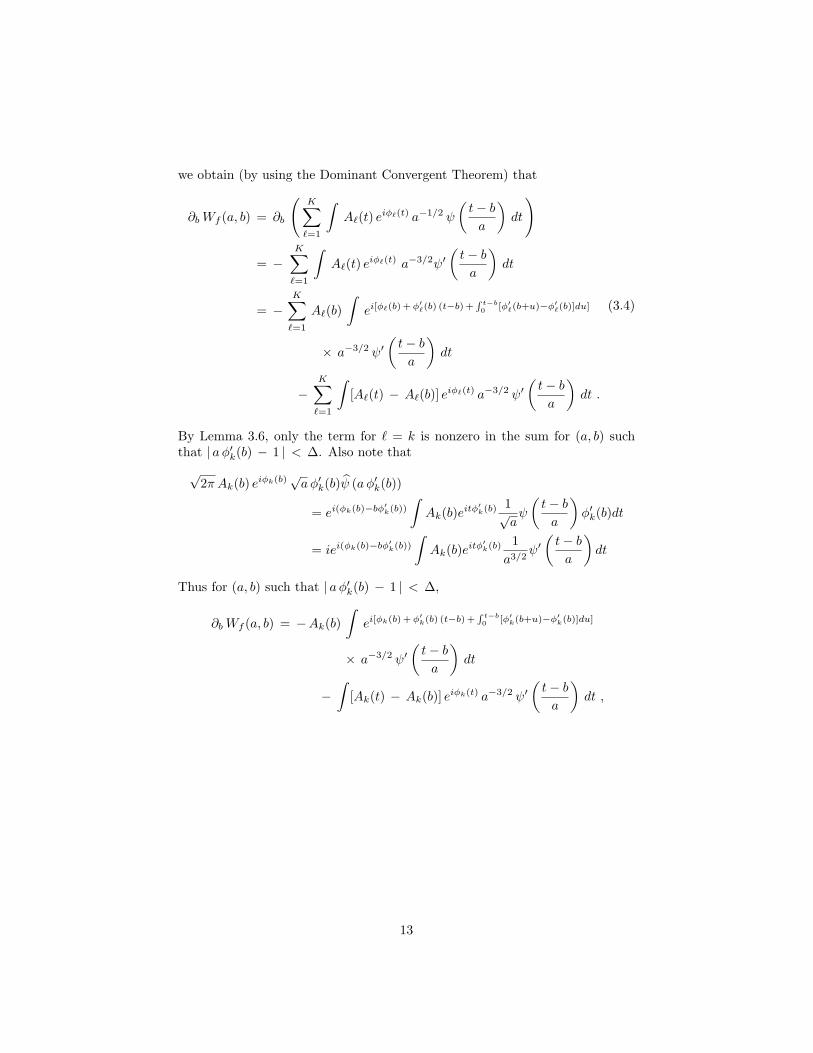
we obtain (by using the Dominant Convergent Theorem) that

∂bWf (a, b) = ∂b

(K∑`=1

∫A`(t) eiφ`(t) a−1/2 ψ

(t− ba

)dt

)

= −K∑`=1

∫A`(t) eiφ`(t) a−3/2ψ′

(t− ba

)dt

= −K∑`=1

A`(b)∫

ei[φ`(b) +φ′`(b) (t−b) +R t−b0 [φ′`(b+u)−φ′`(b)]du]

× a−3/2 ψ′(t− ba

)dt

−K∑`=1

∫[A`(t) − A`(b)] eiφ`(t) a−3/2 ψ′

(t− ba

)dt .

(3.4)

By Lemma 3.6, only the term for ` = k is nonzero in the sum for (a, b) suchthat | aφ′k(b) − 1 | < ∆. Also note that√

2π Ak(b) eiφk(b)√aφ′k(b)ψ (aφ′k(b))

= ei(φk(b)−bφ′k(b))

∫Ak(b)eitφ

′k(b) 1√

aψ

(t− ba

)φ′k(b)dt

= iei(φk(b)−bφ′k(b))

∫Ak(b)eitφ

′k(b) 1

a3/2ψ′(t− ba

)dt

Thus for (a, b) such that | aφ′k(b) − 1 | < ∆,

∂bWf (a, b) = −Ak(b)∫

ei[φk(b) +φ′k(b) (t−b) +R t−b0 [φ′k(b+u)−φ′k(b)]du]

× a−3/2 ψ′(t− ba

)dt

−∫

[Ak(t) − Ak(b)] eiφk(t) a−3/2 ψ′(t− ba

)dt ,

13

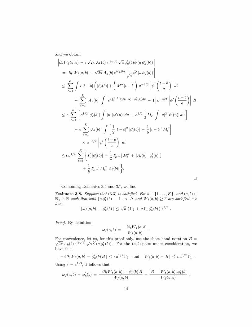
and we obtain∣∣∣∂bWf (a, b) − i√

2π Ak(b) eiφk(b)√aφ′k(b)ψ (aφ′k(b))

∣∣∣=∣∣∣∣∂bWf (a, b) −

√2π Ak(b) eiφk(b) 1√

aψ′ (aφ′k(b))

∣∣∣∣≤

K∑`=1

∫ε |t− b|

(|φ′`(b)|+

12M ′′ |t− b|

)a−3/2

∣∣∣∣ψ′( t− ba)∣∣∣∣ dt

+K∑`=1

|Ak(b)|∫ ∣∣∣ei R t−b

0 [φ′`(b+u)−φ′`(b)]du − 1∣∣∣ a−3/2

∣∣∣∣ψ′( t− ba)∣∣∣∣ dt

≤ ε

K∑`=1

[a1/2 |φ′`(b)|

∫|u| |ψ′(u)| du + a3/2 1

2M ′′`

∫|u|2 |ψ′(u)| du

]

+ ε

K∑`=1

|A`(b)|∫ [

12|t− b|2 |φ′`(b)| +

16|t− b|3M ′′`

]× a−3/2

∣∣∣∣ψ′( t− ba)∣∣∣∣ dt

≤ ε a1/2K∑`=1

I ′1 |φ′`(b)| +

12I ′2 a [M ′′` + |A`(b)| |φ′`(b)| ]

+16I ′3 a

2M ′′` |A`(b)|.

Combining Estimates 3.5 and 3.7, we find

Estimate 3.8. Suppose that (3.3) is satisfied. For k ∈ 1, . . . ,K, and (a, b) ∈R+ × R such that both | aφ′k(b) − 1 | < ∆ and Wf (a, b) ≥ ε are satisfied, wehave

|ωf (a, b) − φ′k(b) | ≤√a ( Γ2 + aΓ1 φ

′k(b) ) ε2/3 .

Proof. By definition,

ωf (a, b) =−i∂bWf (a, b)Wf (a, b)

.

For convenience, let us, for this proof only, use the short hand notation B =√2π Ak(b) eiφk(b)

√a ψ (aφ′k(b)). For the (a, b)-pairs under consideration, we

have then

| − i ∂bWf (a, b) − φ′k(b)B | ≤ ε a1/2 Γ2 and |Wf (a, b)− B | ≤ ε a3/2 Γ1 .

Using ε = ε1/3, it follows that

ωf (a, b) − φ′k(b) =−i∂bWf (a, b) − φ′k(b)B

Wf (a, b)+

[B − Wf (a, b)]φ′k(b)Wf (a, b)

,

14

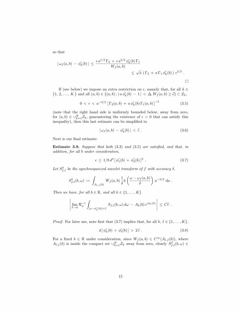
so that

|ωf (a, b) − φ′k(b) | ≤ ε a1/2 Γ2 + ε a3/2 φ′k(b) Γ1

Wf (a, b)

≤√a ( Γ2 + aΓ1 φ

′k(b) ) ε2/3 .

If (see below) we impose an extra restriction on ε, namely that, for all k ∈1, 2, . . . , K and all (a, b) ∈ (a, b) ; | aφ′k(b) − 1 | < ∆,Wf (a, b) ≥ ε ⊂ Zk,

0 < ε < a−3/2 [ Γ2(a, b) + aφ′k(b) Γ1(a, b) ]−3 (3.5)

(note that the right hand side is uniformly bounded below, away from zero,for (a, b) ∈ ∪Kk=1Zk, guaranteeing the existence of ε > 0 that can satisfy thisinequality), then this last estimate can be simplified to

|ωf (a, b) − φ′k(b) | < ε . (3.6)

Next is our final estimate:

Estimate 3.9. Suppose that both (3.3) and (3.5) are satisfied, and that, inaddition, for all b under consideration,

ε ≤ 1/8 d3 [φ′1(b) + φ′2(b) ]3 . (3.7)

Let Sδf,eε be the synchrosqueezed wavelet transform of f with accuracy δ,

Sδf,eε(b, ω) :=∫Aeε,f (b)

Wf (a, b)1δh

(ω − ωf (a, b)

δ

)a−3/2 da .

Then we have, for all b ∈ R, and all k ∈ 1, . . . ,K∣∣∣∣∣ limδ→0R−1ψ

∫|ω−φ′k(b)|<eε Sf,eε(b, ω) dω − Ak(b) eiφk(b)

∣∣∣∣∣ ≤ Cε .

Proof. For later use, note first that (3.7) implies that, for all k, ` ∈ 1, . . . ,K,

d [φ′k(b) + φ′`(b) ] > 2 ε . (3.8)

For a fixed b ∈ R under consideration, since Wf (a, b) ∈ C∞(Aeε,f (b)), whereAeε,f (b) is inside the compact set ∪Kk=1Zk away from zero, clearly Sδf,eε(b, ω) ∈

15

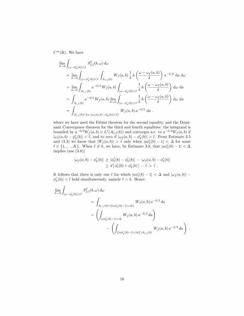
C∞(R). We have

limδ→0

∫|ω−φ′k(b)|<eε S

δf,eε(b, ω) dω

= limδ→0

∫|ω−φ′k(b)|<eε

∫Aeε,f (b)

Wf (a, b)1δh

(ω − ωf (a, b)

δ

)a−3/2 da dω

= limδ→0

∫Aeε,f (b)

a−3/2Wf (a, b)∫|ω−φ′k(b)|<eε

1δh

(ω − ωf (a, b)

δ

)dω da

=∫Aeε,f (b)

a−3/2Wf (a, b) limδ→0

∫|ω−φ′k(b)|<eε

1δh

(ω − ωf (a, b)

δ

)dω da

=∫Aeε,f (b)∩a ; |ωf (a,b)−φ′k(b)|<eε Wf (a, b) a−3/2 da .

where we have used the Fubini theorem for the second equality, and the Domi-nant Convergence theorem for the third and fourth equalities: the integrand isbounded by a−3/2Wf (a, b) ∈ L1(Aeε,f (b)) and converges a.e. to a−3/2Wf (a, b) if|ωf (a, b) − φ′k(b)| < ε, and to zero if |ωf (a, b) − φ′k(b)| > ε. From Estimate 3.5and (3.3) we know that |Wf (a, b)| > ε only when |aφ′`(b) − 1| < ∆ for some` ∈ 1, . . . ,K. When ` 6= k, we have, by Estimate 3.8, that |aφ′`(b) − 1| < ∆implies (use (3.8))

|ωf (a, b)− φ′k(b)| ≥ |φ′`(b)− φ′k(b)| − |ωf (a, b)− φ′`(b)|≥ d [φ′`(b) + φ′k(b) ] − ε > ε .

It follows that there is only one ` for which |aφ′`(b) − 1| < ∆ and |ωf (a, b)| −φ′k(b)| < ε hold simultaneously, namely ` = k. Hence

limδ→0

∫|ω−φ′k(b)|<eε S

δf,eε(b, ω) dω

=∫Aeε,f (b)∩|aφ′k(b)−1|<∆

Wf (a, b) a−3/2 da

=

(∫|aφ′k(b)−1|<∆

Wf (a, b) a−3/2 da

)

−

(∫|aφ′k(b)−1|<∆\Aeε,f (b)

Wf (a, b) a−3/2 da

).

16

From Estimate 3.5 we then obtain∣∣∣∣∣ limδ→0R−1ψ

∫|ω−φ′k(b)|<eε S

δf,eε(b, ω) dω − Ak(b) eiφk(b)

∣∣∣∣∣≤

∣∣∣∣∣R−1ψ

(∫|aφ′k(b)−1|<∆

Wf (a, b) a−3/2 da

)− Ak(b) eiφk(b)

∣∣∣∣∣+ R−1

ψ

∣∣∣∣∣∫|aφ′k(b)−1|<∆\Aeε,f (b)

Wf (a, b) a−3/2 da

∣∣∣∣∣≤

∣∣∣∣∣R−1ψ

√2π Ak(b) eiφk(b)

(∫|aφ′k(b)−1|<∆)

√a ψ(aφ′k(b)) a−3/2 da

)

− Ak(b) eiφk(b)

∣∣∣∣∣+ R−1

ψ

∫|aφ′k(b)−1|<∆)

[ε + ε a−3/2

]da .

The first term on the right hand side vanishes, since

R−1ψ

√2π Ak(b) eiφk(b)

∫|aφ′k(b)−1|<∆

ψ(aφ′k(b)) a−1 da

= R−1ψ

√2π Ak(b) eiφk(b)

∫|ζ−1|<∆

ψ(ζ) ζ−1 dζ = Ak(b) eiφk(b) ,

by the definition of Rψ. In the second term, the integrals can be worked outexplicitly. We thus obtain

∣∣∣∣ limδ→0R−1ψ

∫|ω−φ′k(b)|<eε S

δf,eε(t, ω) dω − Ak(b) eiφk(b)

∣∣∣∣∣≤ 2 εR−1

ψ

[∆

φ′k(b)+(φ′k(b)1−∆

)1/2

−(φ′k(b)1 + ∆

)1/2]

It is now easy to see that all the Estimates together provide a complete prooffor Theorem 3.3.

Remark. We have three different conditions on ε, namely (3.3), (3.5) and (3.7).The auxiliary quantities in these inequalities depend on a and b, and the con-ditions should be satisfied for all (a, b)-pairs under consideration. This is notreally a problem: we saw that the conditions on Ak(b) and φ′k(b) imply thatthere exists an interval of positive measure in which all elements satisfy thethree conditions. Note that the different terms can be traded off in many other

17

ways than what is done here; no effort has been made to optimize the bounds,and they can surely be improved. The focus here was not on optimizing theconstants, but on proving that, if the rate of change (in time) of the Ak(b) andthe φ′k(b) is small, compared with the rate of change of the φk(b) themselves,then synchrosqueezing will identify both the “instantaneous frequencies” andtheir amplitudes.

In the statement of Theorem 3.3, we required the wavelet ψ to be in Schwartzclass and have a compactly supported Fourier transform. These assumptionsare not absolutely necessary; it was done here for convenience in the proof. Forexample, if ψ is not compactly supported, then extra terms occur in many ofthe estimates, taking into account the decay of ψ(ζ) as ζ →∞ or ζ → 0; thesecan be handled in ways similar to what we saw above, at the cost of significantlylengthening the computations without making a conceptual difference.

4. A Variational Approach

The construction and estimates in this section can also be interpreted in avariational framework.

Let us go back to the notion of “instantaneous frequency.” Consider a signals(t) that is a sum of IMT components si(t):

s(t) =N∑i=1

si(t) =N∑i=1

Ai(t) cos(φi(t)), (4.1)

with the additional constraints that φ′i(t) and φ′j(t) for i 6= j are “well sep-arated”, so that it is reasonable to consider the si as individual components.According to the philosophy of EMD, the instantaneous frequency at time t, forthe i-th component, is then given by ωi(t) = φ′i(t).

How could we use this to build a time-frequency representation for s? If werestrict ourselves to a small window in time around T , of the type [T −∆t, T +∆t], with ∆t ≈ 2π/φ′i(T ), then (by its IMT nature) the i-th component can bewritten (approximately) as

si(t) |[T−∆t,T+∆t] ≈ Ai(T ) cos [φi(T ) + φ′i(T ) (t− T )] ,

which is essentially a truncated Taylor expansion in which terms on the orderO(A′i(T )), O(φ′′i (T )) have been neglected. Introducing ωi(T ) = φ′i(T ), and thephase ϕi(T ) := φi(T )− ωi(T )T we can rewrite this as

si(t) |[T−∆t,T+∆t] ≈ Ai(T ) cos [ωi(T )t+ ϕi(T )] .

This signal has a time-frequency representation, as a bivariate “function” oftime and frequency, given by (for t ∈ [T −∆t, T + ∆t])

Fi(t, ω) = Ai(T ) cos[ωt+ ϕi(T )] δ(ω − ωi(T )), (4.2)

18

where δ is the Dirac-delta measure. The time-frequency representation for thefull signal s =

∑Ni=1 si, still in the neighborhood of t = T , would then be

F (t, ω) =N∑i=1

Ai(T ) cos[ωt+ ϕi(T )] δ(ω − ωi(T )). (4.3)

Integrating over ω, in the neighborhood of t = T , leads to s(t) ≈∫F (t, ω) dω.

All this becomes even simpler if we introduce the “complex form” of thetime-frequency representation: for t near T , we have

F (t, ω) =N∑j=1

Aj(T ) exp(iωt) δ(ω − φ′j(T )),

with Aj(T ) = Aj(T ) exp[iϕj(T )]; integration over ω now leads to

Re

[∫F (t, ω) dω

]= Re

N∑j=1

Aj(T ) exp[iωj(T )t+ iϕj(T )]

≈ s(t). (4.4)

Note that, because of the presence of the δ-measure, and under the assumptionthat the components remain separated, the time-frequency function F (t, ω) sat-isfies the equation

∂tF (t, ω) = iωF (t, ω). (4.5)

To get a representation over a longer time-interval, the small pieces de-scribed above have to be knitted together. One way of doing this is to setF (t, ω) =

∑Nj=1 Aj(t) exp(iωt) δ(ω − ωj(t)). This more globally defined F (t, ω)

is still supported on the N curves given by ω = ωj(t), corresponding to theinstantaneous frequency “profile” of the different components. The complex“amplitudes” Aj(t) are given by Aj(t) = Aj(t) exp[iϕj(t)], where, to determinethe phases exp[iϕj(t)], it suffices to know them at one time t0. We have indeed

dϕj(t)dt

=ddt

[φj(t)− ωj(t)t] = φ′j(t)− ωj(t)− ω′j(t)t = −ω′j(t)t;

since the ωj(t) are known (they are encoded in the support of F ), we cancompute the ϕj(t) by using

ϕj(t) = −∫ t

t0

ω′j(τ)τ dτ + ϕj(t0).

Moreover, (4.5) still holds (in the sense of distributions) up to terms of size

19

O(A′i(T )), O(φ′′i (T )), since

∂tF (t, ω) =N∑j=1

[A′j(t)− iω′j(t)tAj(t) + iωAj(t)

]eiωt δ(ω − ωj(t))

+Aj(t) eiωt ω′j(t) δ′(ω − ωj(t))

= iω

N∑j=1

Aj(t) eiωt δ(ω − ωj(t)) + O(A′i(T ), φ′′i (T ))

= iω F (t, ω) + O(A′i(T ), φ′′i (T )).

This suggests modeling the adaptive time-frequency decomposition as a vari-ational problem in which one seeks to minimize∫ ∣∣∣∣Re

[∫F (t, ω)dω

]− s(t)

∣∣∣∣2 dt+ µ

∫∫|∂tF (t, ω)− iωF (t, ω)|2 dtdω (4.6)

to which extra terms could be added, such as, γ∫∫|F (t, ω)|2 dtdω (correspond-

ing to the constraint that F ∈ L2(R2)), or λ∫ [

[∫|F (t, ω)|dω

]2 dt (correspond-ing to a sparsity constraint in ω for each value of t). Using estimates similarto those in Section 3, one can prove that if s ∈ Aε,d, then its synchrosqueezedwavelet transform Ss,eε(b, ω) is close to the minimizer of (4.6). Because the esti-mates and techniques of proof are essentially the same as in Section 3, we don’tgive the details of this analysis here.

Note that wavelets or wavelet transforms play no role in the variationalfunctional – this fits with our numerical observation that although the wavelettransform itself of s is definitely influenced by the choice of ψ, the dependenceon ψ is (almost) completely removed when one considers the synchrosqueezedwavelet transform, at least for signals in Aε,d.

5. Numerical Results

In this section we illustrate the effectiveness of synchrosqueezed wavelettransforms on several examples. For all the examples in this Section, syn-chrosqueezing was carried out starting from a Morlet Wavelet transform; otherwavelets that are well localized in frequency give similar results. The code ofsynchrosqueezing is available upon requests to the authors.

5.1. Instantaneous Frequency Profiles for Synthesized dataWe start by revisiting the toy signal of Figures 1 and 2 in the Introduction.

Figure 6 shows the result of synchrosqueezing the wavelet transform of thistoy signal. We next explore the tolerance to noise of synchrosqueezed wavelettransforms. We denote by X(t) a white noise with zero mean and varianceσ2 = 1. The Signal-to-Noise Ratio (SNR) (measured in dB), will be defined (asusual) by

SNR [dB] = 10 log10

(Var fσ2

),

20

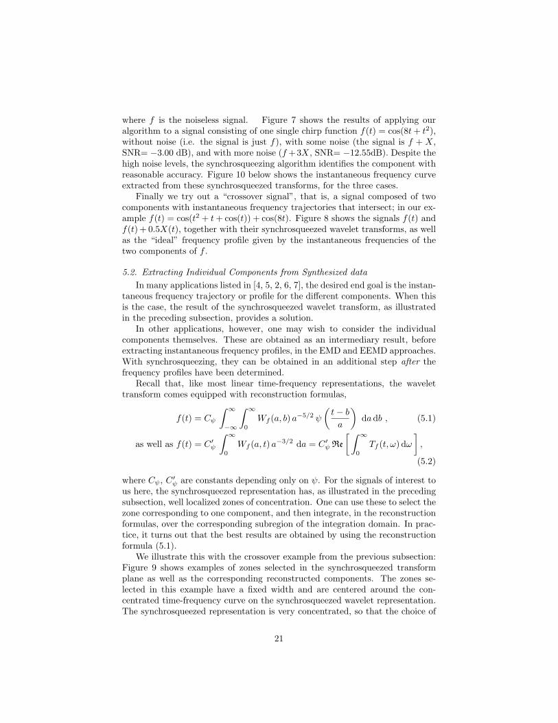
where f is the noiseless signal. Figure 7 shows the results of applying ouralgorithm to a signal consisting of one single chirp function f(t) = cos(8t+ t2),without noise (i.e. the signal is just f), with some noise (the signal is f + X,SNR= −3.00 dB), and with more noise (f +3X, SNR= −12.55dB). Despite thehigh noise levels, the synchrosqueezing algorithm identifies the component withreasonable accuracy. Figure 10 below shows the instantaneous frequency curveextracted from these synchrosqueezed transforms, for the three cases.

Finally we try out a “crossover signal”, that is, a signal composed of twocomponents with instantaneous frequency trajectories that intersect; in our ex-ample f(t) = cos(t2 + t+ cos(t)) + cos(8t). Figure 8 shows the signals f(t) andf(t) + 0.5X(t), together with their synchrosqueezed wavelet transforms, as wellas the “ideal” frequency profile given by the instantaneous frequencies of thetwo components of f .

5.2. Extracting Individual Components from Synthesized dataIn many applications listed in [4, 5, 2, 6, 7], the desired end goal is the instan-

taneous frequency trajectory or profile for the different components. When thisis the case, the result of the synchrosqueezed wavelet transform, as illustratedin the preceding subsection, provides a solution.

In other applications, however, one may wish to consider the individualcomponents themselves. These are obtained as an intermediary result, beforeextracting instantaneous frequency profiles, in the EMD and EEMD approaches.With synchrosqueezing, they can be obtained in an additional step after thefrequency profiles have been determined.

Recall that, like most linear time-frequency representations, the wavelettransform comes equipped with reconstruction formulas,

f(t) = Cψ

∫ ∞−∞

∫ ∞0

Wf (a, b) a−5/2 ψ

(t− ba

)da db , (5.1)

as well as f(t) = C ′ψ

∫ ∞0

Wf (a, t) a−3/2 da = C ′ψ Re

[ ∫ ∞0

Tf (t, ω) dω],

(5.2)

where Cψ, C ′ψ are constants depending only on ψ. For the signals of interest tous here, the synchrosqueezed representation has, as illustrated in the precedingsubsection, well localized zones of concentration. One can use these to select thezone corresponding to one component, and then integrate, in the reconstructionformulas, over the corresponding subregion of the integration domain. In prac-tice, it turns out that the best results are obtained by using the reconstructionformula (5.1).

We illustrate this with the crossover example from the previous subsection:Figure 9 shows examples of zones selected in the synchrosqueezed transformplane as well as the corresponding reconstructed components. The zones se-lected in this example have a fixed width and are centered around the con-centrated time-frequency curve on the synchrosqueezed wavelet representation.The synchrosqueezed representation is very concentrated, so that the choice of

21

the width of the zone is not crucial: the results remain the same for a widerange of choices for this width. This figure also shows the components obtainedfor these signals by EMD for the clean case, and by EEMD (more robust tonoise than EMD) for the noisy case; for this type of signal, the synchrosqueezedtransform proposed here seems to give a more easily interpretable result.

Once the individual components are extracted, one can use them to get anumerical estimate for the variation in time of the instantaneous frequencies ofthe different components. To illustrate this, we revisit the chirp signal fromthe previous subsection. Figure 10 shows the frequency curves obtained by thesynchrosqueezing approach; they are fairly robust with respect to noise.

5.3. Applying the synchrosqueezed transform to some real dataSo far, all the examples shown concerned toy models or synthesized data. In

the subsection we illustrate the result on some real data sets, of medical origin.

5.3.1. Surface Electromyography DataIn this application, we detrend surface electromyography (sEMG) [19] data

acquired from a healthy young female with a portable system (QuickAmp), andexhibit the different IMT componentsmaking up the sEMG signal. The sEMGelectrodes, with sensors of high-purity sintered Ag/AgCl, were placed on thetriceps. The signal was measured for 608 seconds, sampled at 500Hz. Duringthe data acquisition, the subject flexed/extended her elbow, according to aprotocol in which instructions to flex the right or left elbow were given to thesubject at not completely regular time intervals; the subject did not know priorto each instruction which elbow she would be told to flex, and the sequence ofleft/right choices was random. The raw sEMG data sl(t) and sr(t) are shownin the left column in Figure 11.

The middle column in Figure 11 shows the results Ws`(t, ω), Wsr (t, ω) ofour synchrosqueezing algorithm applied to the two sEMG data sets. We used animplementation in which each dyadic scale interval (a ∈ [2k, 2k+1]) was dividedinto 32 equi-log-spaced bins.

The original surface electromyography signals show an erratic drift, whichmedical researchers wish to remove without losing any sharpness in the peaks.To achieve this, we identified the low frequency components (i.e. the dominantcomponents at frequencies below 1 Hz) in the signal, and removed them beforereconstruction. More, precisely, we defined si(t) =

∑ξ≥ξi,cut-off

Tsi(t, ξ), withfrequency cut-off ξi,cut-off(t) = ωi(t) + ω0, where ωi(t) was the dominant com-ponent for signal i (i = ` or r) near 1 Hz with the highest frequency, and ω0

a small constant offset. The right column in Figure 11 shows the results; theerratic drift has disappeared and the peaks are well preserved.

5.3.2. Electrocardiogram DataIn this application we use synchrosqueezing to extract the heart rate variabil-

ity (HRV) from a real electrocardiogram (ECG) signal. The data was acquiredfrom a resting healthy male with a portable ECG machine at sampling rate

22

1000Hz for 600 seconds. The samples were quantized at 12 bits across ±10 mV.The raw ECG data e(t) are (partially) shown in the left half of Figure 12; theright half of the figure shows a blow-up of 20 seconds of the same signal.

The strong, fairly regular spikes in the ECG are called the R peaks; the HRVtime series is defined as the sequence of time differences between consecutiveR peaks. (The interval between two consecutive R peaks is also called the RRinterval.) The HRV is important for both clinical and basic research; it reflectsthe physiological dynamics and state of health of the subject. (See, e.g., [20]for clinical guidelines pertaining to the HRV, and [21] recent advances made inresearch.) The HRV can be viewed as a succession of snapshots of an averagedversion of the instantaneous heart rate.

The left half of Figure 13 shows the synchrosqueezed transform Te(ω, t) ofe(t); in this case we used an implementation in which each dyadic scale interval(a ∈ [2k, 2k+1]) was divided into 128 equi-log-spaced bins. The synchrosqueezedtransform Te(ω, t) has a dominant line c(t) near 1.2Hz, the support of whichcan be parameterized as (t, ωc(t)); t ∈ [0, 80sec] . The right half of Figure 13tracks the dependence on t of ωc(t). This figure also plot a (piecewise constant)function f(t) that tracks the HRV time series and that is computed as follows:if t lies between t− i and ti+1, the locations in time for the i-th and (i + 1)-stR peaks, then f(t) = [ti+1− ti]−1. The plot for ω(t) and f(t) are clearly highlycorrelated.

Acknowledgement: The authors are grateful to the Federal Highway Admin-istration, which supported this research via FHWA grant DTFH61-08-C-00028.They also thank Prof. Norden Huang and Prof. Zhaohua Wu for many stimu-lating discussions and their generosity in sharing their code and insights. Theyalso thank MD. Shu-Shya Hseu and Prof. Yu-Te Wu for providing the realmedical signal. They thank the anonymous referees for useful suggestions ofimproving the presentation of the paper.

[1] P. Flandrin, Time-frequency/time-scale analysis, Vol. 10 of Wavelet Anal-ysis and its Applications, Academic Press Inc., San Diego, CA, 1999, witha preface by Yves Meyer, Translated from French by Joachim Stockler.

[2] N. E. Huang, Z. Shen, S. R. Long, M. C. Wu, H. H. Shih, Q. Zheng, N.-C. Yen, C. C. Tung, H. H. Liu, The empirical mode decomposition andthe Hilbert spectrum for nonlinear and non-stationary time series analysis,Proc. R. Soc. A 454 (1998) 903–995.

[3] N. E. Huang, Z. Wu, S. R. Long, K. C. Arnold, K. Blank, T. W. Liu,On instantaneous frequency, Advances in Adaptive Data Analysis 1 (2009)177–229.

[4] M. Costa, A. A. Priplata, L. A. Lipsitz, Z. Wu, N. E. Huang, A. L. Gold-berger, C.-K. Peng, Noise and poise: enhancement of postural complexityin the elderly with a stochastic-resonance-based therapy, Europhys. Lett.77 (2007) 68008.

23

[5] D. A. Cummings, R. A. Irizarry, N. E. Huang, T. P. Endy, A. Nisalak,K. Ungchusak, D. S. Burke, Travelling waves in the occurrence of denguehaemorrhagic fever in Thailand, Nature 427 (2004) 344–347.

[6] N. E. Huang, Z. Wu, A review on Hilbert-Huang transform: Method andits applications to geophysical studies, Rev. Geophys. 46 (2008) RG2006.

[7] Z. Wu, N. E. Huang, Ensemble empirical mode decomposition: A noise-assisted data analysis method, Advances in Adaptive Data Analysis 1(2009) 1–41.

[8] P. Flandrin, G. Rilling, P. Goncalves, Empirical mode decomposition as afilter bank, IEEE Signal Process. Lett. 11 (2) (2004) 112–114.

[9] Z. Wu, N. E. Huang, A study of the characteristics of white noise usingthe empirical mode decomposition method, Proc. R. Soc. A 460 (2004)1597–1611.

[10] G. Rilling, P. Flandrin, One or two frequencies? The empirical mode de-composition answers, IEEE Trans. Signal Process. 56 (1) (2008) 85–95.

[11] L. Lin, Y. Wang, H. Zhou, Iterative filtering as an alternative algorithmfor empirical mode decomposition, Advances in Adaptive Data Analysis 1(2009) 543–560.

[12] C. Huang, L. Yang, Y. Wang, Convergence of a convolution-filtering-basedalgorithm for empirical mode decomposition, Advances in Adaptive DataAnalysis 1 (2009) 560–571.

[13] I. Daubechies, S. Maes, A nonlinear squeezing of the continuous wavelettransform based on auditory nerve models, in: A. Aldroubi, M. Unser(Eds.), Wavelets in Medicine and Biology, CRC Press, 1996, pp. 527–546.

[14] F. Auger, P. Flandrin, Improving the readability of time-frequency andtime-scale representations by the reassignment method, IEEE Trans. SignalProcess. 43 (5) (1995) 1068–1089.

[15] E. Chassande-Mottin, F. Auger, P. Flandrin, Time-frequency/time-scalereassignment, in: Wavelets and signal processing, Appl. Numer. Harmon.Anal., Birkhauser Boston, Boston, MA, 2003, pp. 233–267.

[16] E. Chassande-Mottin, I. Daubechies, F. Auger, P. Flandrin, Differentialreassignment, Signal Processing Letters, IEEE 4 (10) (1997) 293–294.

[17] I. Daubechies, Ten lectures on wavelets, Vol. 61 of CBMS-NSF RegionalConference Series in Applied Mathematics, Society for Industrial and Ap-plied Mathematics (SIAM), Philadelphia, PA, 1992.

24

[18] N. Delprat, B. Escudie, P. Guillemain, R. Kronland-Martinet,P. Tchamitchian, B. Torresani, Asymptotic wavelet and Gabor analysis:extraction of instantaneous frequencies, Information Theory, IEEE Trans-actions on 38 (2) (1992) 644–664.

[19] J. Cram, G. Kasman, J. Holtz, Introduction to Surface Electromyography,Aspen Publishers Inc., 1998.

[20] M. Malik, A. J. Camm, Dynamic Electrocardiography, Wiley, New York,2004.

[21] S. Cerutti, A. Goldberger, Y. Yamamoto, Recent advances in heart ratevariability signal processing and interpretation, Biomedical Engineering,IEEE Transactions on 53 (1) (2006) 1–3.

25

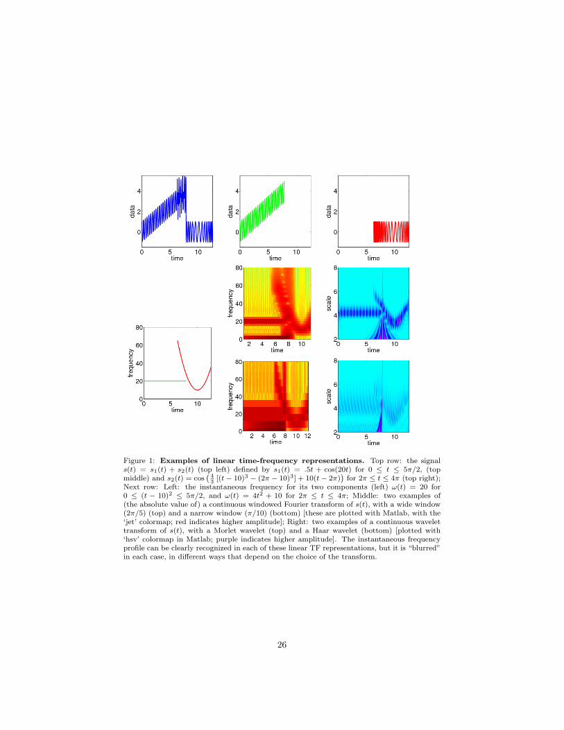
Figure 1: Examples of linear time-frequency representations. Top row: the signals(t) = s1(t) + s2(t) (top left) defined by s1(t) = .5t + cos(20t) for 0 ≤ t ≤ 5π/2, (topmiddle) and s2(t) = cos

`43

[(t− 10)3 − (2π − 10)3] + 10(t− 2π)´

for 2π ≤ t ≤ 4π (top right);Next row: Left: the instantaneous frequency for its two components (left) ω(t) = 20 for0 ≤ (t − 10)2 ≤ 5π/2, and ω(t) = 4t2 + 10 for 2π ≤ t ≤ 4π; Middle: two examples of(the absolute value of) a continuous windowed Fourier transform of s(t), with a wide window(2π/5) (top) and a narrow window (π/10) (bottom) [these are plotted with Matlab, with the‘jet’ colormap; red indicates higher amplitude]; Right: two examples of a continuous wavelettransform of s(t), with a Morlet wavelet (top) and a Haar wavelet (bottom) [plotted with‘hsv’ colormap in Matlab; purple indicates higher amplitude]. The instantaneous frequencyprofile can be clearly recognized in each of these linear TF representations, but it is “blurred”in each case, in different ways that depend on the choice of the transform.

26

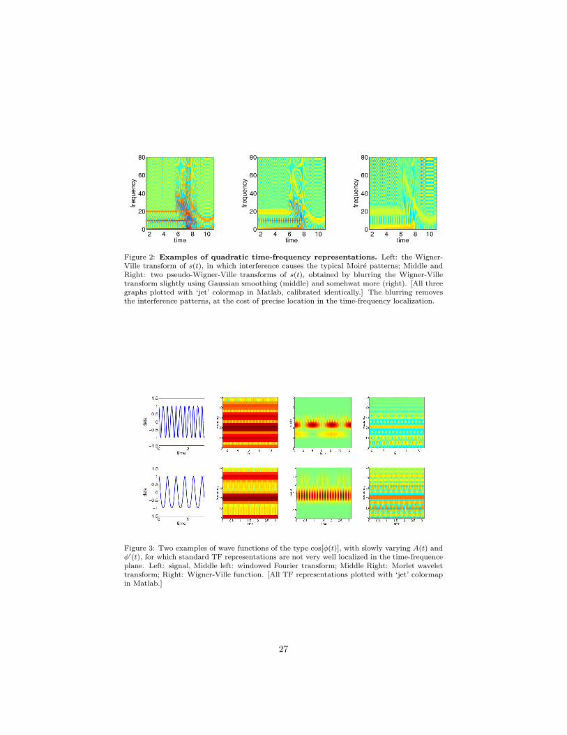
Figure 2: Examples of quadratic time-frequency representations. Left: the Wigner-Ville transform of s(t), in which interference causes the typical Moire patterns; Middle andRight: two pseudo-Wigner-Ville transforms of s(t), obtained by blurring the Wigner-Villetransform slightly using Gaussian smoothing (middle) and somehwat more (right). [All threegraphs plotted with ‘jet’ colormap in Matlab, calibrated identically.] The blurring removesthe interference patterns, at the cost of precise location in the time-frequency localization.

Figure 3: Two examples of wave functions of the type cos[φ(t)], with slowly varying A(t) andφ′(t), for which standard TF representations are not very well localized in the time-frequenceplane. Left: signal, Middle left: windowed Fourier transform; Middle Right: Morlet wavelettransform; Right: Wigner-Ville function. [All TF representations plotted with ‘jet’ colormapin Matlab.]

27

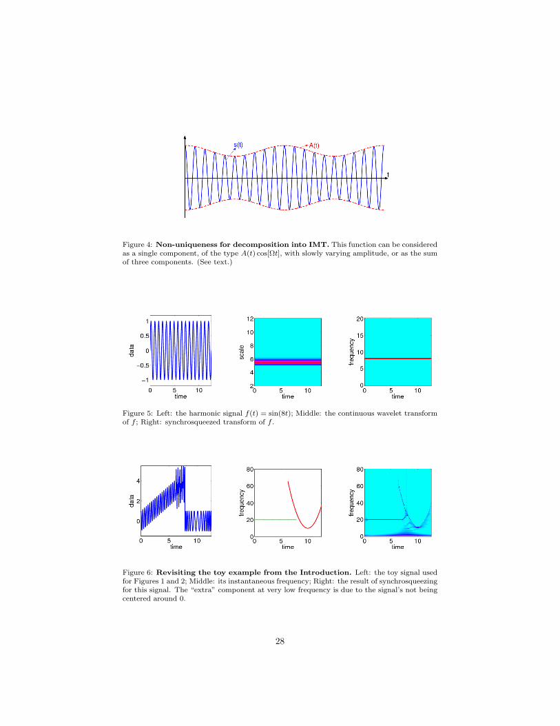
Figure 4: Non-uniqueness for decomposition into IMT. This function can be consideredas a single component, of the type A(t) cos[Ωt], with slowly varying amplitude, or as the sumof three components. (See text.)

Figure 5: Left: the harmonic signal f(t) = sin(8t); Middle: the continuous wavelet transformof f ; Right: synchrosqueezed transform of f .

Figure 6: Revisiting the toy example from the Introduction. Left: the toy signal usedfor Figures 1 and 2; Middle: its instantaneous frequency; Right: the result of synchrosqueezingfor this signal. The “extra” component at very low frequency is due to the signal’s not beingcentered around 0.

28

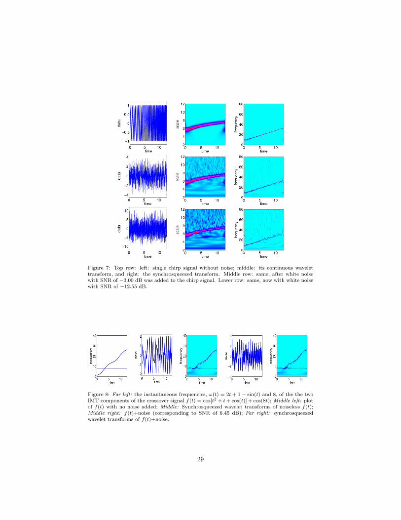
Figure 7: Top row: left: single chirp signal without noise; middle: its continuous wavelettransform, and right: the synchrosqueezed transform. Middle row: same, after white noisewith SNR of −3.00 dB was added to the chirp signal. Lower row: same, now with white noisewith SNR of −12.55 dB.

Figure 8: Far left: the instantaneous frequencies, ω(t) = 2t+ 1− sin(t) and 8, of the the twoIMT components of the crossover signal f(t) = cos[t2 + t+ cos(t)] + cos(8t); Middle left: plotof f(t) with no noise added; Middle: Synchrosqueezed wavelet transforms of noiseless f(t);Middle right: f(t)+noise (corresponding to SNR of 6.45 dB); Far right: synchrosqueezedwavelet transforms of f(t)+noise.

29

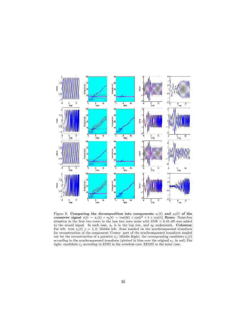
Figure 9: Comparing the decomposition into components s1(t) and s2(t) of thecrossover signal s(t) = s1(t) + s2(t) = cos(8t) + cos[t2 + t + cos(t)] Rows: Noise-freesituation in the first two rows; in the last two rows noise with SNR = 6.45 dB was addedto the mixed signal. In each case, s1 is in the top row, and s2 underneath. Columns:Far left: true sj(t) j = 1, 2; Middle left: Zone marked on the synchrosqueezed transformfor reconstruction of the component; Center: part of the synchrosqueezed transform singledout for the reconstruction of a putative sj ; Middle Right: the corresponding candidate sj(t)according to the synchrosqueezed transform (plotted in blue over the original sj , in red); Farright: candidate sj according to EMD in the noiseless case, EEMD in the noisy case.

30

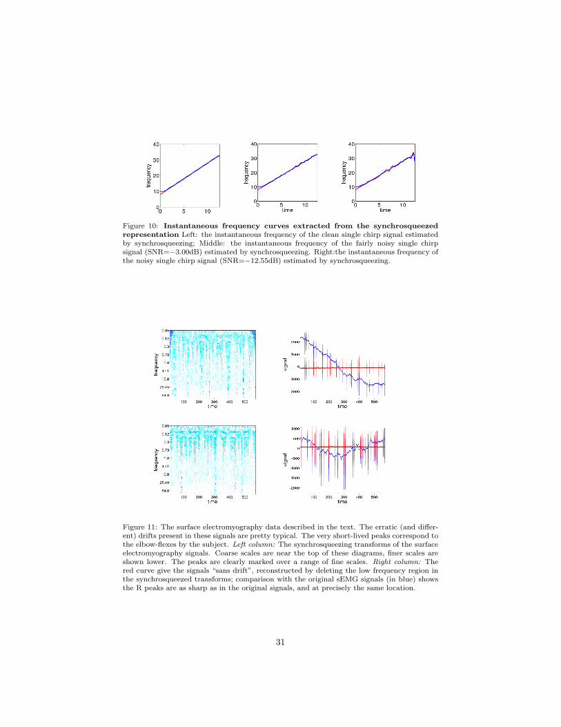
Figure 10: Instantaneous frequency curves extracted from the synchrosqueezedrepresentation Left: the instantaneous frequency of the clean single chirp signal estimatedby synchrosqueezing; Middle: the instantaneous frequency of the fairly noisy single chirpsignal (SNR=−3.00dB) estimated by synchrosqueezing. Right:the instantaneous frequency ofthe noisy single chirp signal (SNR=−12.55dB) estimated by synchrosqueezing.

Figure 11: The surface electromyography data described in the text. The erratic (and differ-ent) drifts present in these signals are pretty typical. The very short-lived peaks correspond tothe elbow-flexes by the subject. Left column: The synchrosqueezing transforms of the surfaceelectromyography signals. Coarse scales are near the top of these diagrams, finer scales areshown lower. The peaks are clearly marked over a range of fine scales. Right column: Thered curve give the signals “sans drift”, reconstructed by deleting the low frequency region inthe synchrosqueezed transforms; comparison with the original sEMG signals (in blue) showsthe R peaks are as sharp as in the original signals, and at precisely the same location.

31

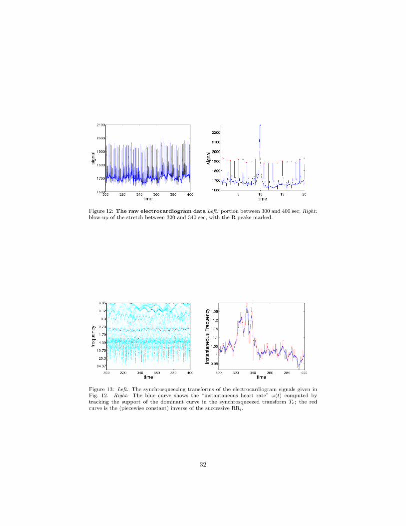
Figure 12: The raw electrocardiogram data Left: portion between 300 and 400 sec; Right:blow-up of the stretch between 320 and 340 sec, with the R peaks marked.

Figure 13: Left: The synchrosqueezing transforms of the electrocardiogram signals given inFig. 12. Right: The blue curve shows the “instantaneous heart rate” ω(t) computed bytracking the support of the dominant curve in the synchrosqueezed transform Te; the redcurve is the (piecewise constant) inverse of the successive RRi.

32