Thesis for the Degree of Licentiate of Philosophy

Symplectic methods for Hamiltonian isospectral

flows and 2D incompressible Euler equations on

a sphere

Milo Viviani

Division of Applied Mathematics and StatisticsDepartment of Mathematical Sciences

Chalmers University of Technology and University of Gothenburg

Goteborg, Sweden 2018

Symplectic methods for Hamiltonian isospectral flows and 2D incompress-

ible Euler equations on a sphere

Milo Viviani

c© Milo Viviani, 2018.

Department of Mathematical SciencesChalmers University of Technology and University of GothenburgSE-412 96 GOTEBORG, SwedenPhone: +46 (0)31 772 1000

Author e-mail: viviani@chalmers.se

Typeset with LATEX.Department of Mathematical SciencesPrinted in Goteborg, Sweden 2018

Symplectic methods for Hamiltonian isospectralflows and 2D incompressible Euler equations on

a sphere

Milo Viviani

Department of Mathematical SciencesChalmers University of Technology and University of Gothenburg

Abstract

The numerical solution of non-canonical Hamiltonian systems is an

active and still growing field of research. At the present time, the biggest

challenges concern the realization of structure preserving algorithms for

differential equations on infinite dimensional manifolds. Several classical

PDEs can indeed be set in this framework. In this thesis, I develop a new

class of numerical schemes for Hamiltonian isospectral flows, in order to

solve the hydrodynamical Euler equations on a sphere. The results are

presented in two papers.

In the first one, we derive a general framework for the isospectral flows,

providing then a class of numerical methods of arbitrary order, based on

the Lie–Poisson reduction of Hamiltonian systems. Avoiding the use of

any constraint, we obtain a large class of numerical schemes for Hamil-

tonian and non-Hamiltonian isospectral flows. One of the advantages of

these methods is that, together with the isospectrality, they have near

conservation of the Hamiltonian and, indeed, they are Lie–Poisson inte-

grators.

In the second paper, using the results of the first one, we present a

numerical method based on the geometric quantization of the Poisson

algebra of the smooth functions on a sphere, which gives an approximate

solution of the Euler equations with a number of discrete first integrals

which is consistent with the level of discretization.

Keywords: Geometric integration, Symplectic methods, Structure preservingalgorithms, Lie–Possion systems, Hamiltonian systems, Isospectral flows, Eulerequations, Fluid dynamics.

List of appended papers

Paper I K. Modin, M. Viviani.Lie–Poisson methods for isospectral flows.Preprint

Paper II M. Viviani.A structure preserving scheme for the Euler equations on a (ro-tating) sphere.Preprint

My contribution to the appended papers:

Paper I: I have developed the numerical methods and most of the theo-retical framework, drafted the manuscript and, after consultation,produced the final manuscript, except for the first two introduc-tory sections. I have implemented the code, under the supervisionof professor K. Modin.

Paper II: Independently developed and written.

iv

Acknowledgements

I would like to thank my supervisor, professor Klas Modin, for the interestingand enlightening discussions and suggestions during the last two and half years,for the good moments around the world.

Heartfelt thanks to professor Stig Larsson, for having always been a referencepoint in these years.

Thank you Anders, a great scientist and a better friend. Thank you Efthymiosfor your ϕιλια and your precious teachings. A great thanks to the ”lunch group”and colleagues: Maximilian, Olof, Simone, Carl, Valentina, Medet, Helga, Chris-tian, Jimmy, Adam, Marten, Johannes, Hanna, Marco, Hung, Geir, Dawan,Matteo, Peter. A special mention, for all the professors, the students and thestaff of Chalmers, with whom I have shared the intellectual hill of Johanneberg.

Thank you also to all the friends in Goteborg: Carlo III, Marco, Antonio,Layla, and all the others that I have met in these years. I remember all of you.

To my family and friends still close, no matter how far, thank you, I simplyowe it all to you.

Milo VivianiGothenburg, May 2018

v

Contents

Introduction 1

History . . . . . . . . . . . . . . . . . . . . . . . . . . . . . . . . . . . . 1Motivation . . . . . . . . . . . . . . . . . . . . . . . . . . . . . . . . . . 2

1 Lie–Poisson systems 3

1.1 Poisson structures and Hamiltonian systems . . . . . . . . . . . . . 31.2 Lie–Poisson systems . . . . . . . . . . . . . . . . . . . . . . . . . . 51.3 Co-adjoint representation . . . . . . . . . . . . . . . . . . . . . . . 61.4 Momentum maps and Lie–Poisson reduction . . . . . . . . . . . . . 8

1.4.1 Lie–Poisson reduction . . . . . . . . . . . . . . . . . . . . . . 91.5 Lie–Poisson systems on gl(n,C)∗ . . . . . . . . . . . . . . . . . . . 10

1.5.1 ad vs ad∗ . . . . . . . . . . . . . . . . . . . . . . . . . . . . . 101.5.2 Euler–Poincare equations and their representations . . . . . . 101.5.3 Lie–Poisson maps on gl(n,C)∗ . . . . . . . . . . . . . . . . . 12

2 Isospectral flows and their numerical solution 14

2.1 Isospectral flows and their properties . . . . . . . . . . . . . . . . . 142.1.1 Restriction to a subspace of gl(n,C) . . . . . . . . . . . . . . 15

2.2 Numerical approximation of the isospectral flows . . . . . . . . . . 15

3 2D Euler equations on the sphere and their numerical solution 17

3.1 Hydrodynamical Euler equations . . . . . . . . . . . . . . . . . . . 173.2 Geometric structure of the Euler equations . . . . . . . . . . . . . . 183.3 Lα-convergence . . . . . . . . . . . . . . . . . . . . . . . . . . . . . 203.4 The reduced system . . . . . . . . . . . . . . . . . . . . . . . . . . 22

3.4.1 With the Coriolis force . . . . . . . . . . . . . . . . . . . . . . 22

4 Summary of the results in the papers 22

4.1 Paper I: Lie–Poisson methods for isospectral flows . . . . . . . . . 224.2 Paper II: A structure preserving scheme for the Euler equations on

a (rotating) sphere . . . . . . . . . . . . . . . . . . . . . . . . . . . 24

5 Proposals for future work 27

5.1 Paper I: Lie–Poisson methods for isospectral flows . . . . . . . . . 275.2 Paper II: A structure preserving scheme for the Euler equations on

a (rotating) sphere . . . . . . . . . . . . . . . . . . . . . . . . . . . 27

Bibliography 28

vi

Introduction

History

The following thesis would like to summarize the last two and half years spenton the study of the numerical solution of Lie–Poisson Hamiltonian systems andtheir connection with other fields of mathematics and applications.

The starting point of the present research dates back to my master thesis,defended in September 2015. In that work I was interested in the numericalsolution of the hydrodynamical Euler equations on a rotating sphere with con-tinuous and singular (point vortices) vorticity fields. The aim of that thesis wasto get a numerical method which retained the main geometric properties of thecontinuous equations in the discrete case. The hydrodynamical Euler equationsare indeed a classical example of Lie–Poisson Hamiltonian system. This meansthat the equations encode a lot of symmetries and therefore conservation laws.What had motivated my research was that there was not yet an established andefficient way to integrate the Euler equations respecting those symmetries.

Eventually that thesis did not give a satisfactory result and the researchhad to be continued during my PhD studies, started in October 2015 under thesupervision of prof. Klas Modin. During the first one and half years the resultsobtained were quite satisfactory but still not really innovative. The main reasonwas that our simulations of the Euler equations required very large matrices andthe algorithm developed still had too many implicit equations to be solved inorder to be really applicable.

Finally, we came to a turning point. In our approach, it was clear that, toretain the first integrals, we needed to put some constraints on the equations.However, what if the constraints could be instead intrinsically encoded into thenumerical method? This was not in general a feasible approach but surprisinglyit turned out that, in this case, aiming for simplicity was rewarding. Workingwith this idea in mind it was possible to generate several numerical methodsmuch simpler and efficient than the previous ones. Moreover a lot of Lie–Poisson systems could then be solved with the same approach and in fact, forany quadratic Lie algebra, it was easy to derive a Lie–Poisson integrator of anyorder. An encouraging fact was also that the methods developed looked like tobe the natural ones, requiring only the information coming from the Lie algebra.

Here I present these results in the following way. In the first section I willintroduce the general framework of Lie–Poisson Hamiltonian systems and someremarks on the Poisson reduction. In section two, the theory and the numericsof isospectral flows will be presented and discussed. In section three I will focuson the numerical solution of the Euler equations on a sphere, which had beenthe main source and aim of the whole research. Finally, I will conclude with asummary of the papers and the aim of future research. In appendix, paper I-II

1

are attached.

Motivation

The problems here presented are a classical and widely studied topic among thegeometric integration community. However, it may (or may not) be surprisingthat several questions are still unsolved. It will be clear while reading thethesis that the work here presented aims to connect different threads, eitherto conclude or complete several papers found in literature. In particular, thetwo main branches of the thesis, i.e., the Hamiltonian isospectral flows andthe incompressible Euler equations, will be connected. The first one will befocused on the possibility of having intrinsic arbitrarily high order methods forHamiltonian isospectral flows. The positive answer obtained will lead to a directapplication to the second one and will provide a better understanding of thepossible advantages of having a Casimir functions-preservation discretizationscheme.

2

1 Lie–Poisson systems

Since its foundation, mathematical physics has been built up from the languageand the concepts coming from geometry. The mechanics of Giuseppe LodovicoLagrangia, Leonard Euler and William Hamilton tried instead to develop ananalytical formulation of the fundamental laws of the Universe. Therefore itwas not expected that the same equations were hiding even more geometrythan before. Sophus Lie, Emmy Noether and lately Vladimir Arnold showedthat the natural language of physics was indeed the differential geometry.

In this section I want to introduce and discuss one of the most intriguing andubiquitous structure arising in differential geometry and mathematical physics,which is named after the French mathematician Simeon Denis Poisson.

1.1 Poisson structures and Hamiltonian systems

Definition 1 (Poisson bracket). Let M be a smooth manifold and C∞(M) thereal vector space of smooth real valued functions defined on M . The Poissonbracket is a bilinear operation ·, · on C∞(M), satisfying the following condi-tions:

• F,G = −G,F skew symmetry;

• F,G ·H = F,G ·H + F,H ·G Leibniz rule;

• F,G, H+ H,F, G+ G,H, F = 0 Jacobi identity.

A mainfold M equipped with a Poisson bracket is said to be a Poissonmanifold. The Poisson bracket can be represented by a form P∈

∧2TM by1:

F,G(x) = Px(dF (x), dG(x))

for any x ∈M .

Definition 2 (Symplectic form). Let M be a smooth manifold. ω ∈∧2

M issaid to be a symplectic form if it is closed and non degenerate, i.e., for anyp ∈M , v ∈ TpM , if for all w ∈ TpM ωp(v, w) = 0, then v = 0.

A manifold M equipped with a symplectic form ω is said to be a symplecticmanifold, and it is denoted as (M,ω).

1Note that we will denote by∧

2 TM the space of the sections from M to the alternating2-tensor on the tangent bundle of M while by

∧2 T ∗M =:

∧2 M the space of the sections

from M to the the alternating 2-tensor on the cotangent bundle of M , which are the usual2-forms.

3

Remark 1. We observe that M always admits a trivial Poisson bracket, i.e.,the zero one, but not always a symplectic form. In fact M has to be of evendimension and orientable (e.g., R2n, n > 0). Moreover, if M is compact, thenthe second group of De Rahm cohomology of M must be non zero (e.g., S2 andTn are symplectic but neither RP

2 nor S2n for n > 1 are). Furthermore, asymplectic form induces a canonical Poisson bracket as we will see below.

Definition 3 (Hamiltonian vector field). Let (M,ω) be a symplectic manifold.A vector field X ∈ TM is said to be Hamiltonian if there exists a functionH ∈ C∞(M) such

ιXω = dH

where ιXω is the contraction of ω by X, i.e., ιX :∧2

M →∧1

M such that, forall p ∈M and v ∈ TpM , ιXωp(v) = ωp(Xp, v).

Remark 2. We observe that (3) are nothing else than the Hamilton equations.In fact, for the sake of simplicity, assumeM = R2n. Then a symplectic form canbe represented in the canonical coordinates q1, ..., qn, p1, ..., pn by the constantskew matrix J ∈ M(2n,R) with coefficients as follows: Jij = 0 if i, j ≤ n ori, j > n, Jij = δij if i > n, j ≤ n and Jij = −δij if i ≤ n, j > n. The dHq,p

can be written as ∇Hq,p and X(q, p) = (q, p), where (q, p) are the flow line ofX from some initial values. So (3) becomes

J · (q, p) = ∇Hq,p,

which are the Hamilton equations after inversion of J .

Furthermore, we observe that ω induces a diffeomorphismω : TM → T ∗M defined as ω(v) = ωp(v, ·) for every v ∈ TpM . So, givenF , we define the Hamiltonian vector field associate to F as XF = ω−1(dF ). Fi-nally, given a symplectic manifold (M,ω), we define, for every F,G ∈ C∞(M)the following Poisson bracket:

F,G = ω(XF , XG),

where everything is defined pointwise. To compute (1.1) in local coordinates weneed the following basic theorem.

Theorem 1 (Darboux). Let (M,ω) be a symplectic manifold of dimension 2n.Then for every p ∈ M , there exists a local chart (V, ϕ = (q1, ..., qn, p1, ..., pn))centred in p, such that:

ω|V =∑ni=1 dqi ∧ dpi,

i.e., ω is represented by the matrix J defined above.

4

Such coordinates are called canonical or Darboux coordinates. Now we canwrite (1.1) in coordinates. Let (V, ϕ) be a chart given by the Darboux theorem,then, in this chart, XF =

∑ni=1

∂F∂pi

∂∂qi

− ∂F∂qi

∂∂pi

. A similar expression holds for

XG. Then, a straightforward computation leads to write (1.1) as:

F,G =

n∑

i=1

∂F

∂qi

∂G

∂pi−∂F

∂pi

∂G

∂qi,

where the relations dqi(∂qi) = 1, dqi(∂pi) = 0, dpi(∂qi) = 0, dpi(∂pi) = 1, fori = 1, ...n, have been used. The canonical coordinates satisfy:

qi, qj = pi, pj = 0 and qi, pj = −pj, qi = δij for i, j = 1, ..., n.

An obvious consequence is that, for every F ∈ C∞(M), and any Hamiltonianvector field XH we have:

XH(F ) = F,H.

So for pi, qi, i = 1, ..., n integral curves of XH we have that:

qi = XH(qi) = qi, H and pi = XH(pi) = pi, H for i = 1, ..., n,

which is an other formulation of the Hamilton equations (2).

Definition 4. Let (M,ω,H) be a Hamiltonian system, i.e., a symplectic man-ifold with a Hamiltonian function H. A function f ∈ C∞(M) constant on anyintegral curve of XH is said to be a first integral of the system. A vector fieldX ∈ TM is said to be an infinitesimal symmetry if both ω and H are invariantunder the flow of X.

Theorem 2 (Noether theorem). Let (M,ω,H) be a Hamiltonian system.

• if f is a first integral, then Xf is an infinitesimal symmetry;

• on the other hand, if H1(M) = 0 (where H1(M) is the first group of DeRham cohomology of M), then any infinitesimal symmetry is a Hamilto-nian vector field of a first integral, uniquely defined, except for an additiveconstant for any connected component of M .

1.2 Lie–Poisson systems

A remarkable Poisson structure can be naturally given to the vector spacesthat are also the dual of a Lie algebra. Consider a Lie algebra (g, [·, ·]), not

5

necessarily of finite dimension, and let g∗ be its dual. Then on C∞(g∗) we havethe following (canonical) Poisson bracket:2

F,G±(v) = ±〈v, [dF (v), dG(v)]〉

where v ∈ g∗ and we have identified g ∼= g∗∗.The Lie–Poisson bracket is a very important example of a generally neither

trivial nor symplectic Poisson bracket. In this case, the Poisson form P ∈∧2

Tg∗

is linear and can be expressed by:

Pij(v) = ±Ckijvk

where Ckij are the structure constants of g. Let H be a smooth function on g∗.Then, the system:

F (v(t)) = F,H±(v(t))F (v(0)) = F (v0)

which has to be satisfied for any F ∈ C∞(g∗), it is said to be Lie–Poissonsystem with Hamiltonian function H (the bracket is the one defined above andv(t) ∈ g∗, for any t ∈ R). Because of the anti-commutativity of the Poissonbracket, it is clear that in a Lie–Poisson system the Hamiltonian is a conservedquantity in time. Moreover, depending on the rank of the form defining thebracket, we have a certain number of first integrals of the motion, that arethe same for any Hamiltonian. These functions that commute with any otherone, i.e., C, · = 0 are called Casimir functions. As we will discuss in thenext sections, the preservation of the Casimir functions and the Hamiltonianby a numerical method is crucial in the applications in order to guarantee goodpredictions for long times.

1.3 Co-adjoint representation

We want now express (1.2) in terms of the co-adjoint representation of a Liealgebra. We have first to recall some definitions.

Let G be a Lie group, and consider the map

C : G×G −→ G

(g, h) 7→ Cg(h) := ghg−1.

Then, for each g ∈ G, we have the internal automorphism Cg. If we takethe differential of this map in the identity e we get the adjoint representation,Ad of G in End(g), that is defined by:

2The ± sign depends on the fact that the Poisson bracket here defined can also be obtainedvia the reduction of the canonical ones on the left (-) or right (+) invariant functions on T ∗G

(see section 1.4.1 below).

6

Adg(X) =d

dt |t=0(g exptX g−1), ∀g ∈ G,X ∈ g.

Finally, differentiating Ad : G → End(g) and identifying End(g) with itstangent, we obtain the map:

ad :g −→ End(g)

X 7→ adX = [X, ·].

Let us now define the dual of the adjoint representation, i.e., the represen-tation of the group G and the Lie algebra g on the endomorphism of the dual ofthe Lie algebra g∗. We define the co-adjoint representation Ad∗ : G→ End(g∗)by:

〈Ad∗(g)(φ), X〉 = 〈φ,Ad(g−1)X〉 ∀g ∈ G,X ∈ g, φ ∈ g∗.

Proceeding as before, one can find the infinitesimal version ad∗ : g →

End(g∗), given by ad∗X = −(adX)∗, i.e.,

〈ad∗X(φ), Y 〉 = 〈φ,−adX(Y )〉 ∀X,Y ∈ g, φ ∈ g∗.

Let O be an orbit of the co-adjoint action Ad∗ : G × g∗ → g∗. It holds theremarkable fact that the co-adjoint orbits have a canonical symplectic structure,called Kirillov-Kostant-Souriau form. Let p ∈ O and X,Y ∈ g, then the twoform:

ωp(ad∗X(p), ad∗Y (p)) = 〈p, [X,Y ]〉,

is a symplectic form on O, where we have used the canonical identification of g∗∗

with g, from which we have obtained that T∗g∗ ≃ g∗× g. We conclude noticingthat the co-adjoint orbits are immersed submanifold3 where the Casimir func-tions are constant. However, in general, the Casimir functions don’t characterizethe co-adjoint orbits4.

Let us go back to the Lie–Poisson system (1.2). We notice that the bracketcan be expressed in terms of the co-adjoint representation of g:

±〈v, [dF (v), dH(v)]〉 = ∓〈v, addH(v)(dF (v))〉 = ±〈ad∗dH(v)(v), dF (v)〉.

We want to remark that a Lie–Poisson system evolves precisely on the co-adjoint orbits given by the Ad∗ action. In fact let consider F = F (v(t)) wherex(t) is a curve in g∗, and v(0) = v0. Applying the chain rule we get:

dF (v) = ±〈ad∗dH(v)(v), dF (v)〉

3If the action of the group G is also proper, e.g., G compact, then the co-adjoint orbits areembedded submanifold.

4[13], pag. 479.

7

for any F ∈ C∞(g∗). Hence it is true that:

v = ±ad∗dH(v)(v).

Integrating this system we get:

v(t) = Ad∗exp(±

∫t

0dH(v(s))ds)(v0).

1.4 Momentum maps and Lie–Poisson reduction

In this section we will briefly recall the concept and the main properties of themomentum map of a group action on a Poisson manifold. For further detailswe refer to [12] and [13].

Let G be a Lie group acting to the left on a Poisson manifold P , such thatfor any g ∈ G the action Φg is a Poisson map, i.e., ·, · Φg = · Φg, · Φg.Let the infinitesimal action of G be the map ρ : g× P → TP defined by:

ρξ(p) =d

dt |t=0exp(tξ)p,

for any ξ ∈ g, p ∈ P . Hence, ρξ is a vector field on P . Furthermore, we assumethe G-action to be Hamiltonian, i.e., there exists a function Jξ ∈ C∞(P ) suchthat ρξ = ·, Jξ. Then we define the momentum map µ : P → g∗ by:

〈µ(p), ξ〉 = Jξ(p).

We remark that, if the Poisson bracket is induced by a symplectic form ω, thenthe momentum map can be defined by the formula:

d〈µ(p), ξ〉 = ιρξ(p)ωp.

For a right action one can repeat exactly the same calculations. The maindifference, as one can easily check, is that the map J : g → C∞(P) is a Liealgebra homomorphism for the left action and a Lie algebra anti-morphism forthe right action (cfr. [12]).

Let us now denote µL (respectively µR) the momentum map coming fromthe left (respectively right) G-action on P . Let also g∗− (respectively g∗+) bethe dual of the Lie algebra g endowed with the − (respectively +) Lie–Poissonbracket.

The main property of the momentum maps is stated in the following propo-sition:

Proposition 1 (Prop 2.1, [12]). Let µL : P → g∗+ (respectively µR : P → g∗−)be the momentum map defined above. Then µL (respectively µR) is a Poissonmap.

8

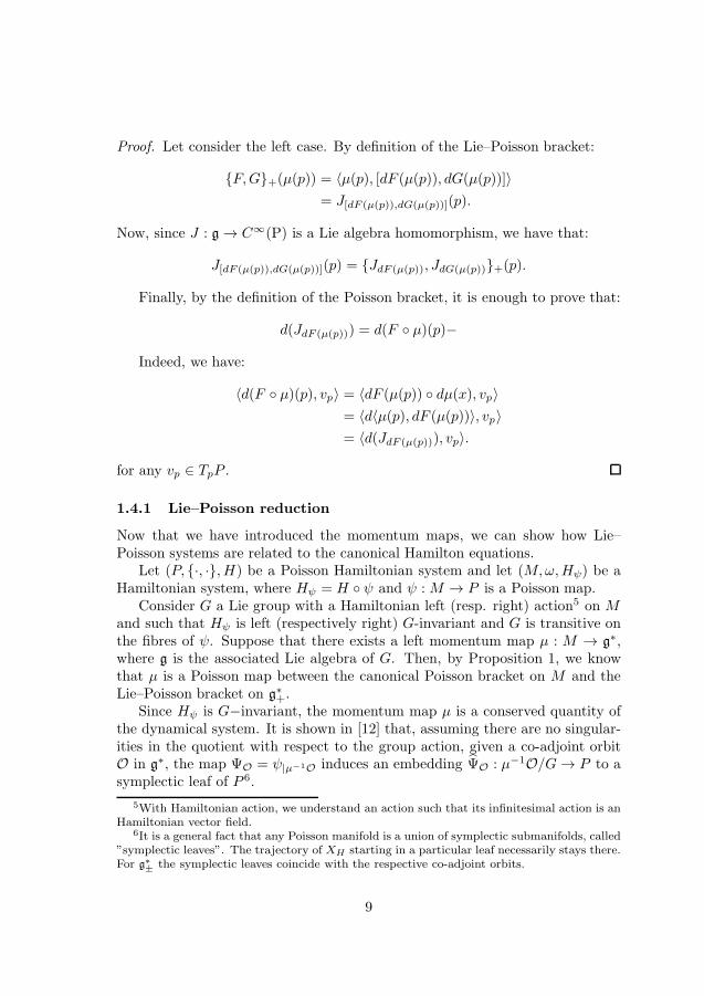
Proof. Let consider the left case. By definition of the Lie–Poisson bracket:

F,G+(µ(p)) = 〈µ(p), [dF (µ(p)), dG(µ(p))]〉

= J[dF (µ(p)),dG(µ(p))](p).

Now, since J : g → C∞(P) is a Lie algebra homomorphism, we have that:

J[dF (µ(p)),dG(µ(p))](p) = JdF (µ(p)), JdG(µ(p))+(p).

Finally, by the definition of the Poisson bracket, it is enough to prove that:

d(JdF (µ(p))) = d(F µ)(p)−

Indeed, we have:

〈d(F µ)(p), vp〉 = 〈dF (µ(p)) dµ(x), vp〉

= 〈d〈µ(p), dF (µ(p))〉, vp〉

= 〈d(JdF (µ(p))), vp〉.

for any vp ∈ TpP .

1.4.1 Lie–Poisson reduction

Now that we have introduced the momentum maps, we can show how Lie–Poisson systems are related to the canonical Hamilton equations.

Let (P, ·, ·, H) be a Poisson Hamiltonian system and let (M,ω,Hψ) be aHamiltonian system, where Hψ = H ψ and ψ :M → P is a Poisson map.

Consider G a Lie group with a Hamiltonian left (resp. right) action5 on Mand such that Hψ is left (respectively right) G-invariant and G is transitive onthe fibres of ψ. Suppose that there exists a left momentum map µ : M → g∗,where g is the associated Lie algebra of G. Then, by Proposition 1, we knowthat µ is a Poisson map between the canonical Poisson bracket on M and theLie–Poisson bracket on g∗+.

Since Hψ is G−invariant, the momentum map µ is a conserved quantity ofthe dynamical system. It is shown in [12] that, assuming there are no singular-ities in the quotient with respect to the group action, given a co-adjoint orbitO in g∗, the map ΨO = ψ|µ−1O induces an embedding ΨO : µ−1O/G→ P to asymplectic leaf of P 6.

5With Hamiltonian action, we understand an action such that its infinitesimal action is anHamiltonian vector field.

6It is a general fact that any Poisson manifold is a union of symplectic submanifolds, called”symplectic leaves”. The trajectory of XH starting in a particular leaf necessarily stays there.For g∗± the symplectic leaves coincide with the respective co-adjoint orbits.

9

In particular, when M = T ∗G and P = g∗− (resp. P = g∗+), we can takeΨ = µR (resp. µL) and µ = µL (resp. µR). Then, the canonical Hamilton

equations in T ∗G w.r.t to the Hamiltonian H become the equations (1.2) on g∗−

(resp. g∗+) with respect to to the Hamiltonian H on g∗, defined by H µL = H

(resp. H µR = H).

1.5 Lie–Poisson systems on gl(n,C)∗

In this section, in view of the applications, we want to remark some facts aboutLie–Poisson systems on the dual of the general matrix Lie algebra gl(n,C)∗. Inparticular, we want to clarify in detail the meaning of the identification betweengl(n,C)∗ and gl(n,C) and how this affects the representation of the equationsof a Lie–Poisson system.

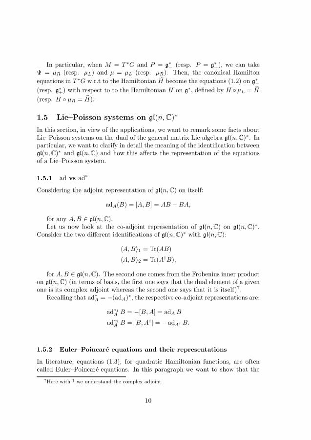
1.5.1 ad vs ad∗

Considering the adjoint representation of gl(n,C) on itself:

adA(B) = [A,B] = AB −BA,

for any A,B ∈ gl(n,C).Let us now look at the co-adjoint representation of gl(n,C) on gl(n,C)∗.

Consider the two different identifications of gl(n,C)∗ with gl(n,C):

〈A,B〉1 = Tr(AB)

〈A,B〉2 = Tr(A†B),

for A,B ∈ gl(n,C). The second one comes from the Frobenius inner producton gl(n,C) (in terms of basis, the first one says that the dual element of a givenone is its complex adjoint whereas the second one says that it is itself)7.

Recalling that ad∗A = −(adA)∗, the respective co-adjoint representations are:

ad∗1

A B = −[B,A] = adAB

ad∗2

A B = [B,A†] = − adA† B.

1.5.2 Euler–Poincare equations and their representations

In literature, equations (1.3), for quadratic Hamiltonian functions, are oftencalled Euler–Poincare equations. In this paragraph we want to show that the

7Here with † we understand the complex adjoint.

10

dynamics generated is independent from the identification of gl(n,C)∗ withgl(n,C).

To define the Euler–Poincare equations, we need a symmetric positive-definite linear map A : gl(n,C) → gl(n,C)∗. An explicit form of this mapdepends on the way we identify the algebra with its dual. Let us denote A withA and A, the respective form, with respect to ad∗2 and respectively, ad∗1 . Wethen have that the following inner products are identically defined:

〈A,B〉A := 〈AA,B〉2 = Tr(((AA)†B)=

〈A,B〉A := 〈AA,B〉1 = Tr(AAB).

for A,B ∈ gl(n,C). Therefore, we have to have that A = † A. Then, forΨ ∈ gl(n,C), the Lagrangian function can be defined as:

L(Ψ) =1

2〈Ψ,Ψ〉A =

1

2〈Ψ,Ψ〉A.

The respective momentum variables in gl(n,C)∗ are:

ΩA =∂L(Ψ)

∂Ψ= AΨ

ΩA =

(∂L(Ψ)

∂Ψ

)†

= AΨ

and we observe that (ΩA)† = ΩA. From these calculations, we get the

Hamiltonian functions:

HA(ΩA) =1

2〈ΩA,A

−1ΩA〉2

HA(ΩA) =1

2〈ΩA, A

−1ΩA〉1.

So we have the identities:

∂HA(ΩA)

∂ΩA= A−1ΩA = Ψ

∂HA(ΩA)

∂ΩA

= A−1ΩA = Ψ.

Finally, we get the equation of motion ([13], Chapt. 13):

〈Ψ, Y 〉A = −〈Ψ, adΨ Y 〉A = 〈A−1 ad∗2

Ψ AΨ, Y 〉A,

〈Ψ, Y 〉A = 〈Ψ, adΨ Y 〉A = −〈A−1 ad∗1

Ψ AΨ, Y 〉A,

11

for any Y ∈ gl(n,C). These can also be written in the strong form as:

Ψ = A−1 ad∗2

Ψ AΨ = A−1[AΨ,Ψ†],

Ψ = A−1 ad∗1

Ψ AΨ = −A−1[AΨ,Ψ],

or, considering the dual version for ΩA,ΩA:

ΩA = ad∗2

A−1ΩAΩA = [ΩA, (A

−1ΩA)†],

ΩA = ad∗1

A−1ΩA

ΩA = −[ΩA, A−1ΩA].

Remark If we transpose the second equation, we get:

Ω†

A= [Ω†

A, (A−1ΩA)

†],

and, using the fact that (ΩA)† = ΩA, and A−1ΩA = A−1ΩA, we see that the

Euler–Poincare equations are independent from the choice of the pairing.

1.5.3 Lie–Poisson maps on gl(n,C)∗

Consider the identification of gl(n,C) with its dual, via the Frobenius pairing.After this identification, the Lie–Poisson structure on gl(n,C)∗ is completelydetermined by the structure constants of gl(n,C). Therefore any Lie algebramorphism of gl(n,C) will be a Lie Poisson map on gl(n,C)∗ and viceversa.

We now want to check how it looks with respect to ad∗. Let consider a :gl(n,C) → gl(n,C) invertible Lie algebra morphism, A,B ∈ gl(n,C) and φ ∈

gl(n,C)∗ ≡ gl(n,C) (via the Frobenius identification). Then we get:

Tr((a ad∗A(φ))†B) = −Tr((a[A†, φ])†B)

= −Tr(φ†[A, a†B])

= −Tr((aφ)†[a−TA,B])

= −Tr(([A†a−1, aφ])†B)

= Tr((ad∗a−TA(aφ))†B).

So we have the formula:

a ad∗A(φ) = ad∗a−TA(aφ).

Consider A to be equal to ∇H(φ), for a smooth function H defined ongl(n,C)∗, i.e., we have a Lie–Poisson Hamiltonian system. Then the action onan invertible linear map on the (Lie–Poisson) Hamiltonian vector field is:

a ·XH := Da XH a−1,

12

where XH(φ) = ad∗∇H(φ)(φ). Then, using the formula (1.5.3), we get:

a ·XH(φ) = a ad∗∇H(a−1φ)(a−1φ)

= ad∗a−T∇H(a−1φ)(φ)

= ad∗∇(Ha−1)(φ)(φ)

= XHa−1(φ),

which is again a Lie–Poisson Hamiltonian system.

13

2 Isospectral flows and their numerical solution

2.1 Isospectral flows and their properties

The isospectral flows are a central class of dynamical systems with symmetries.They arise in fact in different contexts: Lie–Poisson reduction, matrix factor-ization, Lax pairs of integrable systems, et cetera [8],[10],[16]. As the namesuggests, isospectral flows represent a dynamical system on linear operatorssuch that the spectrum of operator is fixed during the whole evolution. If theoperators are diagonalizable, then, at each time, the operator is similar to theinitial one.

Let the flowΦ : [0,∞)× L(V ) → L(V )

(t,W ) 7→ Φt(W )

be an isospectral flow on L(V ), where V is a finite dimensional vector space ofdimension n. Let W0 be the initial value. Then, for any t ≥ 0, there exists U(t)such that:

W (t) = Φt(W0) = U(t)−1W0U(t).

By differentiation of (2.1), one find that W is the solution of:

W = [B(W ),W ]W (0) =W0,

where B(W ) = U−1U and the bracket is the usual matrix commutator [A,B] =AB −BA.

Other than the eigenvalues of the operator, one can choose a different set ofgenerators for the first integrals of (2.1). This is provided by the momentum ofW . In fact:

d

dtTr(W k) = Tr(W k−1[B(W ),W ]) = Tr(B(W )[W k−1,W ]) = 0,

for k = 1, 2, ... . SinceW is represented by a n×nmatrix, its first nmomentaare independent, then they are related by the Cayley–Hamilton theorem (in factTr(W k) =

∑ni=1 λ

ki , for λi the eigenvalues of W ).

When B(W ) takes the form of (the transpose of) a gradient of a function, theequation (2.1) will be said Hamiltonian-Isospectral flow. The word Hamiltonianis because the function H such that B = −∇H† is a conserved quantity of (2.1).In fact:

d

dtH(W ) = −Tr(∇H(W )†[∇H(W )†,W ]) = −Tr(W [∇H(W )†,∇H(W )†]) = 0.

14

A further reason to use the word Hamiltonian is that L(V ), endowed withthe bracket [·, ·], can be seen as the Lie algebra gl(n,C) and the equations (2.1)as the reduced form of a canonical Hamiltonian system, as shown in section1.4.1.

Indeed, if we identify the dual of gl(n,C) with itself, via the Frobeniusinner product 〈A,B〉 = Tr(A†B), the equations (2.1) above form a Lie–PoissonHamiltonian system with respect to the co-adjoint representation of gl(n,C) ongl(n,C)∗ given by:

ad∗AB = [B,A†] = − adA† B

for A ∈ gl(n,C), B ∈ gl(n,C)∗ ∼= gl(n,C).

2.1.1 Restriction to a subspace of gl(n,C)

It is interesting, both for theoretical and practical purposes, to analyse thecase when W evolves on a subspace S of gl(n,C). It is clear that if W ∈ S

then B(W ) has to be in n(S), i.e., the normalizer of S in gl(n,C), which isthe largest subalgebra of gl(n,C) such that [n(S), S] ⊆ S. This framework isused in Paper I to encompass at the same time the ”classical” isospectral flows,e.g., W ∈ Sym(n), B(W ) ∈ o(n), and the Lie–Poisson systems on reductiveLie-algebras.

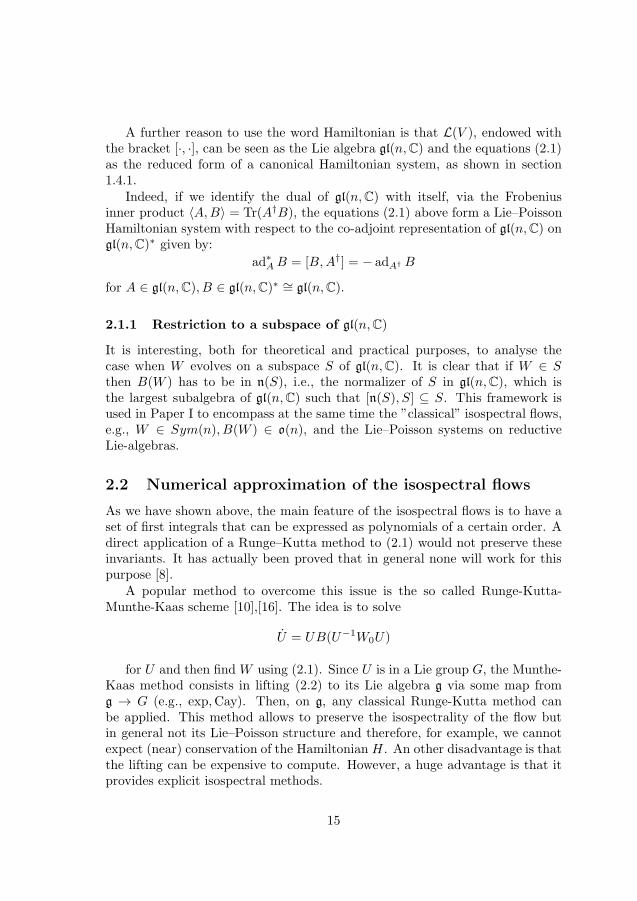
2.2 Numerical approximation of the isospectral flows

As we have shown above, the main feature of the isospectral flows is to have aset of first integrals that can be expressed as polynomials of a certain order. Adirect application of a Runge–Kutta method to (2.1) would not preserve theseinvariants. It has actually been proved that in general none will work for thispurpose [8].

A popular method to overcome this issue is the so called Runge-Kutta-Munthe-Kaas scheme [10],[16]. The idea is to solve

U = UB(U−1W0U)

for U and then find W using (2.1). Since U is in a Lie group G, the Munthe-Kaas method consists in lifting (2.2) to its Lie algebra g via some map fromg → G (e.g., exp,Cay). Then, on g, any classical Runge-Kutta method canbe applied. This method allows to preserve the isospectrality of the flow butin general not its Lie–Poisson structure and therefore, for example, we cannotexpect (near) conservation of the Hamiltonian H . An other disadvantage is thatthe lifting can be expensive to compute. However, a huge advantage is that itprovides explicit isospectral methods.

15

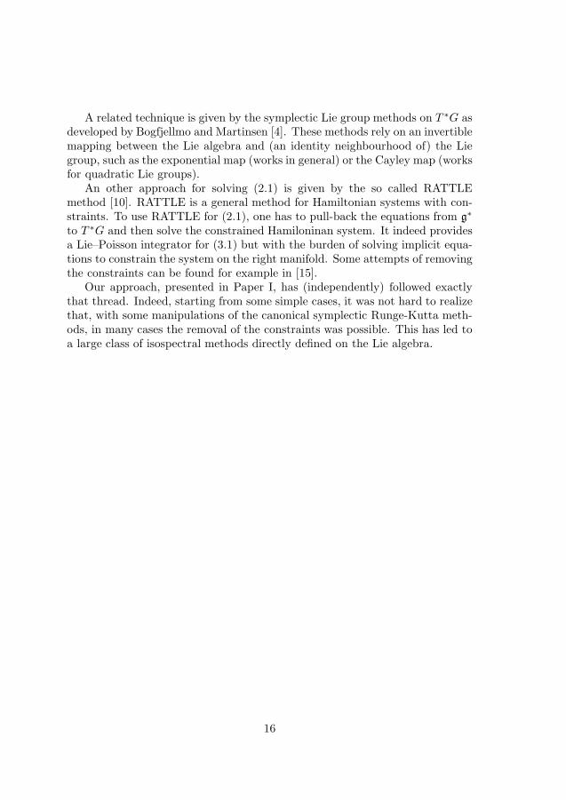
A related technique is given by the symplectic Lie group methods on T ∗G asdeveloped by Bogfjellmo and Martinsen [4]. These methods rely on an invertiblemapping between the Lie algebra and (an identity neighbourhood of) the Liegroup, such as the exponential map (works in general) or the Cayley map (worksfor quadratic Lie groups).

An other approach for solving (2.1) is given by the so called RATTLEmethod [10]. RATTLE is a general method for Hamiltonian systems with con-straints. To use RATTLE for (2.1), one has to pull-back the equations from g∗

to T ∗G and then solve the constrained Hamiloninan system. It indeed providesa Lie–Poisson integrator for (3.1) but with the burden of solving implicit equa-tions to constrain the system on the right manifold. Some attempts of removingthe constraints can be found for example in [15].

Our approach, presented in Paper I, has (independently) followed exactlythat thread. Indeed, starting from some simple cases, it was not hard to realizethat, with some manipulations of the canonical symplectic Runge-Kutta meth-ods, in many cases the removal of the constraints was possible. This has led toa large class of isospectral methods directly defined on the Lie algebra.

16

3 2D Euler equations on the sphere and theirnumerical solution

3.1 Hydrodynamical Euler equations

Consider a homogeneous, incompressible, inviscid, two-dimensional fluid whichis constrained to move on a spherical surface, embedded in the standard Eu-clidean R3, which is rotating with constant angular speed, with respect to afixed normal axis. The equations of motion of such a fluid are given by the wellknown Euler equations of hydrodynamics:

v + v · ∇v = −∇p− 2Ω× v

∇ · v = 0

where v is the velocity vector field of the fluid, p is its internal pressure andΩ = (Ω · n)n is the projection of the angular rotation of the sphere Ω to thenormal n at a point of the sphere. The last term in the first equation of (3.1),

Fc = −2Ω× v is called Coriolis force.The geometry behind this system turns out to play a central role in under-

standing the behaviour of the fluid [2], [3], [12] and in the investigation of nu-merical methods to solve it [1], [14], [17], [18]. In particular the Euler equations(3.1) can be equivalently expressed in terms of the one form v as a Lie–Poissonsystem on the dual of the infinite-dimensional Lie-algebra of divergence-freevector fields. The respective Poisson tensor is degenerate so that there is aninfinite number of independent first integrals (Casimir functions) [3].

On the other hand, an equivalent formulation of (3.1) is given in terms ofthe vorticity ω = (∇× v) · n. We notice that by the Stokes’ theorem it must bethat

∫ω = 0. Then the Euler equations (3.1) can be written as:

ω = ψ, ω

∆ψ = ω − f,

where f = 2Ω·n and ψ is the unique solution to the Poisson equation in C∞(S2),such that

∫ψ = 0.

In this form the Euler equations are a Lie–Poisson system on the smoothfunctions on the sphere which integrate to 0. The Hamiltonian is given by

H(ω) =1

2

∫(ω − f)ψ.

The (infinitely many) Casimir functions are given, for any smooth f , byF (ω) =

∫f(ω). In fact, it is easy to check:

d

dt

∫f(ω) = −

∫f ′(ω)v · ∇ω = −

∫v · ∇f(ω) =

∫(∇ · v)f(ω) = 0,

17

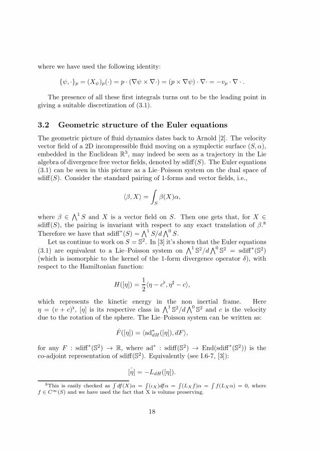
where we have used the following identity:

ψ, ·p = (Xψ)p(·) = p · (∇ψ ×∇·) = (p×∇ψ) · ∇· = −vp · ∇ · .

The presence of all these first integrals turns out to be the leading point ingiving a suitable discretization of (3.1).

3.2 Geometric structure of the Euler equations

The geometric picture of fluid dynamics dates back to Arnold [2]. The velocityvector field of a 2D incompressible fluid moving on a symplectic surface (S, α),embedded in the Euclidean R

3, may indeed be seen as a trajectory in the Liealgebra of divergence free vector fields, denoted by sdiff(S). The Euler equations(3.1) can be seen in this picture as a Lie–Poisson system on the dual space ofsdiff(S). Consider the standard pairing of 1-forms and vector fields, i.e.,

〈β,X〉 =

∫

S

β(X)α,

where β ∈∧1

S and X is a vector field on S. Then one gets that, for X ∈

sdiff(S), the pairing is invariant with respect to any exact translation of β.8

Therefore we have that sdiff∗(S) =∧1

S/d∧0

S.

Let us continue to work on S = S2. In [3] it’s shown that the Euler equations

(3.1) are equivalent to a Lie–Poisson system on∧1

S2/d∧0

S2 = sdiff∗(S2)(which is isomorphic to the kernel of the 1-form divergence operator δ), withrespect to the Hamiltonian function:

H([η]) =1

2〈η − c, η♯ − c〉,

which represents the kinetic energy in the non inertial frame. Hereη = (v + c), [η] is its respective class in

∧1S2/d

∧0S2 and c is the velocity

due to the rotation of the sphere. The Lie–Poisson system can be written as:

F ([η]) = 〈ad∗dH([η]), dF 〉,

for any F : sdiff∗(S2) → R, where ad∗ : sdiff(S2) → End(sdiff∗(S2)) is theco-adjoint representation of sdiff(S2). Equivalently (see I.6-7, [3]):

˙[η] = −LdH([η]).

8This is easily checked as∫df(X)α =

∫(ιX)dfα =

∫(LXf)α =

∫f(LXα) = 0, where

f ∈ C∞(S) and we have used the fact that X is volume preserving.

18

where L is the Lie derivative. In our case, we have dH = η♯ − c = v. Hence:

˙[η] = −Lv([η]).

Note that Lie–Poisson system above defined is respect to the dual pairingin sdiff(S2), being dF ∈ (sdiff∗(S2))∗ ∼= sdiff(S2).

At this point, to get rid off the equivalence class, one just needs to take theexterior derivative of (3.2) and, using the fact that [Lv, d] = 0, get the Eulerequations in the vorticity form:

β = −Lvβ,

where β = d[η] ∈∧2

S2 represents the vorticity of v.We write the vorticity in terms of the volume form α such that β = qα,

where the q ∈ C∞(S2) and has zero mean. Then we get

Lvβ = Lv(qα) = (Lvq)α+ qLvα = (Lvq)α,

being v volume preserving.By taking the Hodge star of (3.2), via the identification

∧2S2 ∼=

∧0S2 =

C∞(S2), we can understand (3.2) in C∞0 (S2), i.e., the space of smooth functions

which integrate to 0. Hence, we get a map ∗d : sdiff∗(S2) → C∞0 (S2) between

a Lie–Poisson algebra and a Poisson algebra. If we call ad∗ the Lie–Poissonstructure in sdiff∗(S2) and ad the Poisson structure in C∞

0 (S2), then we have:

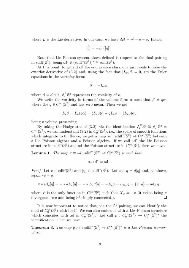
Lemma 1. The map π ≡ ∗d : sdiff∗(S2) → C∞0 (S2) is such that

π∗ ad∗ = ad .

Proof. Let v ∈ sdiff(S2) and [η] ∈ sdiff∗(S2). Let call q = d[η] and, as above,again ∗q = q.

π ad∗v[η] = − ∗ dLv[η] = − ∗ Lvd[η] = −Lvq = LXψq = ψ, q = adψ q,

where ψ is the only function in C∞0 (S2) such that Xψ = −v (it exists being v

divergence free and being S2 simply connected.).

It is now important to notice that, via the L2 pairing, we can identify thedual of C∞

0 (S2) with itself. We can also endow it with a Lie–Poisson structurewhich coincides with ad in C∞

0 (S2). Let call p : C∞0 (S2) → C∞

0 (S2)∗ theidentification. Then we have:

Theorem 3. The map p π : sdiff∗(S2) → C∞0 (S2)∗ is a Lie–Poisson isomor-

phism.

19

Proof. This follows immediately from the Lemma above and the fact thatad∗ψ q = −(adψ q)

∗ = adψ q, which is due to the fact:

∫(v · ∇f)g +

∫f(v · ∇g) =

∫v · ∇(fg) = −

∫∇ · v(fg) = 0

and the equivalence:

〈(adψ q)∗, g〉 = −

∫(v · ∇q)g =

∫q(v · ∇g) = 〈q,− adψ g〉.

As we have seen in the previous paragraph, a consequence of the Eulerequations of being a Lie–Poisson system is that there exists an infinite numberof independent first integrals or Casimir functions. This fact turns out to bethe leading point in giving a suitable spatial discretization of the system. Infact, while solving the equations with a numerical scheme, we cannot expectto preserve all the infinite first integrals but what we do want to get is havingan increasing number of first integrals with respect to the size of the discreteproblem. This cannot be achieved by simply considering a truncated spectraldecomposition of the vorticity [17], [18].

Instead we used the approach proposed by Zeitlin in [18], based on thetheory of geometric quantization of compact Kahler manifolds [6], [5], [11]. Itprovides a sequence of finite-dimensional twisted-representations of the infinite-dimensional Lie algebra of divergence-free vector fields, sdiff(S2). This sequencecan also be seen as a finite dimensional approximation of sdiff(S2), in the senseof the Lα-convergence, which will be explained below. Then, for any of thosequasi-representations, we get a finite dimensional analogue of (3.1), i.e., a Lie–Poisson Hamiltonian system on su(n) (or sl(n,C)), for any n ≥ 1, with n − 1independent Casimir functions.

3.3 Lα-convergence

Let us consider a Lie-algebra (g, [·, ·]) and a family of labelled Lie algebras(gα, [·, ·]α)α∈I , where α ∈ I = N or R. Furthermore, assume then that to anyelement of this family it is associated a distance dα and a surjective projectionmap pα : g → gα. Then we will say that (g, [·, ·]) is an Lα-approximation of(gα, [·, ·]α)α∈I if:

• if x, y ∈ g and dα(pα(x), pα(y)) → 0, for α → ∞, then x = y,

• for all x, y ∈ g we have dα(pα([x, y]), [pα(x), pα(y)]α) → 0, for α → ∞,

• all pα, for α ≫ 0, are surjective.

20

The above definition is given in [5] and it is a quite weak requirement to geta limit for a sequence of Lie algebras. Indeed the same sequence may convergein the Lα sense to different Lie algebras [6]. Much depends on the choice of theprojections that are not canonical. However, for our purposes, since we havealready a target and we need a suitable sequence to approximate it, we won’tneed more than that.

Let us now consider the smooth complex functions with 0 mean on thesphere, and denote them with C∞

0 (S2,C). This vector space can be canonicallyendowed by a Poisson structure given by the respective Hamiltonian vectorfields of two functions and a symplectic form α on S2. We have, for any f, g ∈

C∞0 (S2,C):

f, g = α(Xf , Xg).

With this bracket, C∞0 (S2,C) becomes an infinite dimensional Poisson alge-

bra. A basis is given by the complex spherical harmonics, which will be denotedin the standard notation and azimuthal-inclination coordinates (φ, θ) as:

Ylm =

√2l+ 1

4π

(l −m)!

(l +m)!Pml (cos θ)eimφ,

for l ≥ 1 and m = −l, . . . , l. In this basis it has been built up by J. Hoppe [11]and fully proved (even in a more general contest) by M. Bordemann, E. Mein-renken and M. Schlichenmaier [5] an explicit Lα-approximating sequence, givenby the matrix Lie algebra (sl(n,C), [·, ·]n)n∈N , where [·, ·]n = n3/2[·, ·], therescaled usual commutator of matrices.

The distances are given by a suitable matrix norm and the projections aredefined by associating to any spherical harmonic a respective matrix, for anyn ∈ N, i.e., pn : Ylm 7→ T nlm, where

(T nlm)m1m2= (−1)n/2−m1

√2l+ 1

(n/2 l n/2−m1 m m2

),

where the round bracket is the Wigner 3j-symbols. The result can be summa-rized as:

Theorem 4 (Bordemann, Hoppe, Meinrenken, Schlichenmaier [6],[5]). Let usconsider the Poisson algebra (C∞

0 (S2,C), ·, ·) whose pairing is defined in (3.3).Then with respect to pn defined above and dn any matrix norm, we have that(C∞

0 (S2,C), ·, ·) is an Lα-approximation of (sl(n,C), [·, ·]n)n∈N.

21

3.4 The reduced system

We can now derive the spatial discretization of the Euler equations via theLα-approximation. We first present the system without the Coriolis force.

For any n ∈ N, we get an analogous of the Euler equations (3.1):

W = [∆−1n W,W ]n,

where W ∈ sl(n,C) and ∆−1n is the inverse of the discrete Laplacian as defined

in [18]. The crucial property of ∆−1n is that ∆−1

n T nlm = (−l(l + 1))−1T nlm, forany l = 1, ..., n, m = −l, ..., l.

We remark that, for a real valued vorticity, W is actually in su(n), whichmeans that W lm = (−1)mWl−m.

The discrete Hamiltonian takes the following form:

H(W ) =1

2Tr(∆−1

n WW †).

The discrete system has the following independent n− 1 of first integrals9

Fn(W ) = Tr(W k) for k=2,..,n

which, up to a normalization constant dependent on n, converge to the powersof the continuous vorticity.

3.4.1 With the Coriolis force

In the case with the Coriolis force, the discrete system is:

W = [∆−1n (W − F ),W ]n,

where F = 2ΩT n10 represents the discrete Coriolis force.The discrete Hamiltonian in this case takes the following form:

H(W ) =1

2Tr(∆−1

n (W − F )(W − F )†).

4 Summary of the results in the papers

4.1 Paper I: Lie–Poisson methods for isospectral flows

In paper I, we treat isospectral flows and Lie–Poisson systems together, whichlead to a general recipe for solving both numerically, capturing their main geo-metrical features.

9One should notice that by definition Tr(W ) = 0 for all W ∈ sl(n,C) and Tr(Wn) can bereplaced by det(W ), by the Cayley–Hamilton theorem.

22

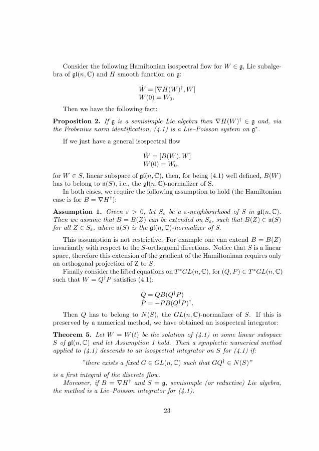
Consider the following Hamiltonian isospectral flow for W ∈ g, Lie subalge-bra of gl(n,C) and H smooth function on g:

W = [∇H(W )†,W ]W (0) =W0.

Then we have the following fact:

Proposition 2. If g is a semisimple Lie algebra then ∇H(W )† ∈ g and, viathe Frobenius norm identification, (4.1) is a Lie–Poisson system on g∗.

If we just have a general isospectral flow

W = [B(W ),W ]W (0) =W0,

for W ∈ S, linear subspace of gl(n,C), then, for being (4.1) well defined, B(W )has to belong to n(S), i.e., the gl(n,C)-normalizer of S.

In both cases, we require the following assumption to hold (the Hamiltoniancase is for B = ∇H†):

Assumption 1. Given ε > 0, let Sε be a ε-neighbourhood of S in gl(n,C).Then we assume that B = B(Z) can be extended on Sε, such that B(Z) ∈ n(S)for all Z ∈ Sε, where n(S) is the gl(n,C)-normalizer of S.

This assumption is not restrictive. For example one can extend B = B(Z)invariantly with respect to the S-orthogonal directions. Notice that S is a linearspace, therefore this extension of the gradient of the Hamiltoninan requires onlyan orthogonal projection of Z to S.

Finally consider the lifted equations on T ∗GL(n,C), for (Q,P ) ∈ T ∗GL(n,C)such that W = Q†P satisfies (4.1):

Q = QB(Q†P )

P = −PB(Q†P )†.

Then Q has to belong to N(S), the GL(n,C)-normalizer of S. If this ispreserved by a numerical method, we have obtained an isospectral integrator:

Theorem 5. Let W = W (t) be the solution of (4.1) in some linear subspaceS of gl(n,C) and let Assumption 1 hold. Then a symplectic numerical methodapplied to (4.1) descends to an isospectral integrator on S for (4.1) if:

”there exists a fixed G ∈ GL(n,C) such that GQ† ∈ N(S)”

is a first integral of the discrete flow.Moreover, if B = ∇H† and S = g, semisimple (or reductive) Lie algebra,

the method is a Lie–Poisson integrator for (4.1).

23

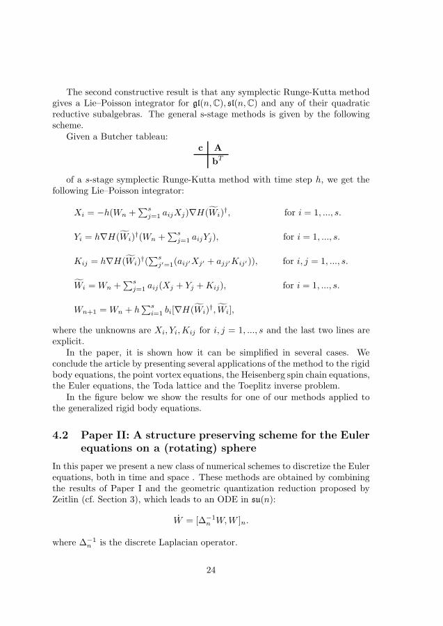
The second constructive result is that any symplectic Runge-Kutta methodgives a Lie–Poisson integrator for gl(n,C), sl(n,C) and any of their quadraticreductive subalgebras. The general s-stage methods is given by the followingscheme.

Given a Butcher tableau:c A

bT

of a s-stage symplectic Runge-Kutta method with time step h, we get thefollowing Lie–Poisson integrator:

Xi = −h(Wn +∑s

j=1 aijXj)∇H(Wi)†, for i = 1, ..., s.

Yi = h∇H(Wi)†(Wn +

∑sj=1 aijYj), for i = 1, ..., s.

Kij = h∇H(Wi)†(∑s

j′=1(aij′Xj′ + ajj′Kij′ )), for i, j = 1, ..., s.

Wi =Wn +∑s

j=1 aij(Xj + Yj +Kij), for i = 1, ..., s.

Wn+1 =Wn + h∑si=1 bi[∇H(Wi)

†, Wi],

where the unknowns are Xi, Yi,Kij for i, j = 1, ..., s and the last two lines areexplicit.

In the paper, it is shown how it can be simplified in several cases. Weconclude the article by presenting several applications of the method to the rigidbody equations, the point vortex equations, the Heisenberg spin chain equations,the Euler equations, the Toda lattice and the Toeplitz inverse problem.

In the figure below we show the results for one of our methods applied tothe generalized rigid body equations.

4.2 Paper II: A structure preserving scheme for the Eulerequations on a (rotating) sphere

In this paper we present a new class of numerical schemes to discretize the Eulerequations, both in time and space . These methods are obtained by combiningthe results of Paper I and the geometric quantization reduction proposed byZeitlin (cf. Section 3), which leads to an ODE in su(n):

W = [∆−1n W,W ]n.

where ∆−1n is the discrete Laplacian operator.

24

Hamiltonian variation

Eigenvalues variation

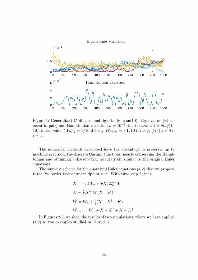
Figure 1: Generalized 45-dimensional rigid body in so(10). Eigenvalues (whichoccur in pair) and Hamiltonian variation; h = 10−1; inertia tensor I = diag(1 :10); initial value (W0)ij = 1/10 if i < j, (W0)ij = −1/10 if i > j, (W0)ij = 0 ifi = j.

The numerical methods developed have the advantage to preserve, up tomachine precision, the discrete Casimir functions, nearly conserving the Hamil-tonian and obtaining a discrete flow qualitatively similar to the original Eulerequations.

The simplest scheme for the quantized Euler equations (4.2) that we proposeis the 2nd order isospectral midpoint rule. With time step h, it is:

X = −h(Wn + 12X)∆−1

n W

K = h2∆

−1n W (X +K)

W =Wn + 12 (X −X† +K)

Wn+1 =Wn +X −X† +K −K†.

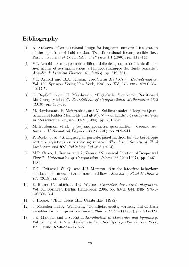
In Figures 2-3, we show the results of two simulations, where we have applied(4.2) to two examples studied in [9] and [7].

25

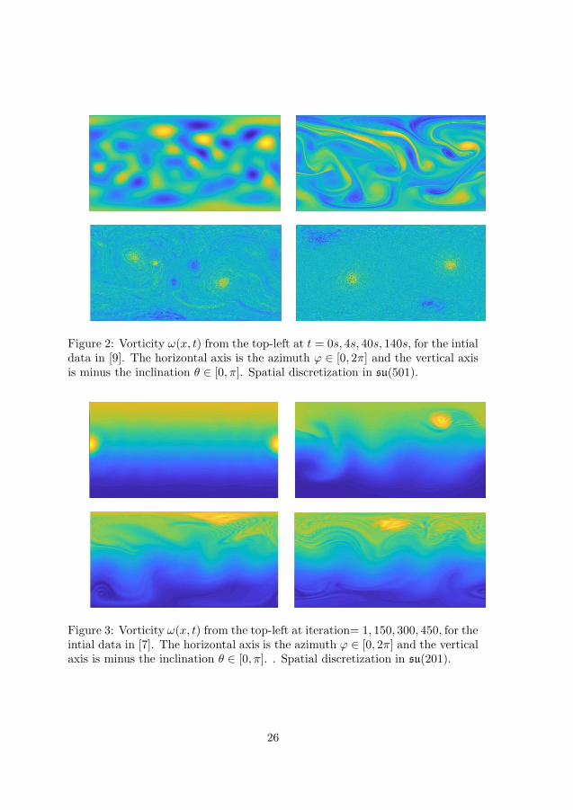
Figure 2: Vorticity ω(x, t) from the top-left at t = 0s, 4s, 40s, 140s, for the intialdata in [9]. The horizontal axis is the azimuth ϕ ∈ [0, 2π] and the vertical axisis minus the inclination θ ∈ [0, π]. Spatial discretization in su(501).

Figure 3: Vorticity ω(x, t) from the top-left at iteration= 1, 150, 300, 450, for theintial data in [7]. The horizontal axis is the azimuth ϕ ∈ [0, 2π] and the verticalaxis is minus the inclination θ ∈ [0, π]. . Spatial discretization in su(201).

26

5 Proposals for future work

5.1 Paper I: Lie–Poisson methods for isospectral flows

In Paper I, we presented a general approach for solving numerically Lie–Poissonsystems on reductive Lie algebras. In view of the Levi decomposition of fi-nite dimensional Lie algebras, i.e., that any of them can be decomposed into asemi-direct product of a semisimple and a solvable Lie subalgebra, it would beinteresting to develop analogous results for Lie–Poisson systems on solvable Liealgebras.

5.2 Paper II: A structure preserving scheme for the Eulerequations on a (rotating) sphere

In paper II, encouraging results in the study of the Euler equations have beenshown. However, our simulations, despite good, should be implemented withhigher resolution, in order to give more reliable predictions.

Analogously, a full analysis of the convergence of the quantized equationsto the original one is still missing and it should be accomplished to understandthe quality of such an approximation.

Last but not least, simulations of coupled continuous and singular vorticity(point vortices) have yet to be done.

27

Bibliography

[1] A. Arakawa. “Computational design for long-term numerical integrationof the equations of fluid motion: Two-dimensional incompressible flow.Part I”. Journal of Computational Physics 1.1 (1966), pp. 119–143.

[2] V.I. Arnold. “Sur la geometrie differentielle des groupes de Lie de dimen-sion infinie et ses applications a l’hydrodynamique del fluids parfaits”.Annales de l’institut Fourier 16.1 (1966), pp. 319–361.

[3] V.I. Arnold and B.A. Khesin. Topological Methods in Hydrodynamics.Vol. 125. Springer-Verlag New York, 1998, pp. XV, 376. isbn: 978-0-387-94947-5.

[4] G. Bogfjellmo and H. Marthinsen. “High-Order Symplectic PartitionedLie Group Methods”. Foundations of Computational Mathematics 16.2(2016), pp. 493–530.

[5] M. Bordemann, E. Meinrenken, and M. Schlichenmaier. “Toeplitz Quan-tization of Kahler Manifolds and gl(N), N → ∞ limits”. Communicationsin Mathematical Physics 165.2 (1994), pp. 281–296.

[6] M. Bordemann et al. “gl(∞) and geometric quantization”. Communica-tions in Mathematical Physics 138.2 (1991), pp. 209–244.

[7] P. Bosler et al. “A Lagrangian particle/panel method for the barotropicvorticity equations on a rotating sphere”. The Japan Society of FluidMechanics and IOP Publishing Ltd 46.3 (2014).

[8] M.P. Calvo, A. Iserles, and A. Zanna. “Numerical Solution of IsospectralFlows”. Mathematics of Computation Volume 66.220 (1997), pp. 1461–1486.

[9] D.G. Dritschel, W. Qi, and J.B. Marston. “On the late-time behaviourof a bounded, inviscid two-dimensional flow”. Journal of Fluid Mechanics783 (2015), pp. 1–22.

[10] E. Hairer, C. Lubich, and G. Wanner. Geometric Numerical Integration.Vol. 31. Springer, Berlin, Heidelberg, 2006, pp. XVII, 644. isbn: 978-3-540-30663-4.

[11] J. Hoppe. “Ph.D. thesis MIT Cambridge” (1982).

[12] J. Marsden and A. Weinstein. “Co-adjoint orbits, vortices, and Clebschvariables for incompressible fluids”. Physica D 7.1–3 (1983), pp. 305–323.

[13] J.E. Marsden and T.S. Ratiu. Introduction to Mechanics and Symmetry.Vol. vol. 17 of Texts in Applied Mathematics. Springer-Verlag, New York,1999. isbn: 978-0-387-21792-5.

28

[14] R. McLachlan. “Explicit Lie–Poisson Integration and the Euler Equa-tions”. Physical review letters 71.19 (1993), pp. 3043–3046.

[15] R. McLachlan and C. Scovel. “Equivariant constrained symplectic inte-gration”. Journal of Nonlinear Science 5.3 (1995), pp. 233–256.

[16] M. Webb. “Isospectral algorithms, Toeplitz matrices and orthogonal poly-nomials, Ph.D. thesis” (2017).

[17] V. Zeitlin. “Finite-mode analogues of 2D ideal hydrodynamics: Coadjointorbits and local canonical structure”. Physica D 49.3 (1991), pp. 353–362.

[18] V. Zeitlin. “Self-Consistent-Mode Approximation for the Hydrodynam-ics of an Incompressible Fluid on Non rotating and Rotating Spheres”.Physical review letters 93.26 (2004), pp. 353–362.

29