Sylvia Richardson Centre for Biostatistics Imperial College, London
69
1 Sylvia Richardson Centre for Biostatistics Imperial College, London Bayesian hierarchical modelling of genomic data In collaboration with Natalia Bochkina, Anne Mette Hein, Alex Lewin (St Mary’s) Helen Causton and Tim Aitman (Hammersmith) Peter Green (Bristol) Philippe Broët (INSERM, Paris) BBSRC Exploiting Genomics grant
-
Upload
kelly-meyer -
Category
Documents
-
view
27 -
download
0
description
Bayesian hierarchical modelling of genomic data. Sylvia Richardson Centre for Biostatistics Imperial College, London. In collaboration with Natalia Bochkina, Anne Mette Hein, Alex Lewin (St Mary’s) Helen Causton and Tim Aitman (Hammersmith) Peter Green (Bristol) - PowerPoint PPT Presentation
Transcript of Sylvia Richardson Centre for Biostatistics Imperial College, London
1
Sylvia RichardsonCentre for Biostatistics
Imperial College, London
Bayesian hierarchical modelling of genomic data
In collaboration with Natalia Bochkina, Anne Mette Hein, Alex Lewin (St Mary’s)
Helen Causton and Tim Aitman (Hammersmith)Peter Green (Bristol)
Philippe Broët (INSERM, Paris)
BBSRC Exploiting Genomics grant

2
Outline
• Introduction
• A fully Bayesian gene expression index (BGX)
• Differential expression and array effects
• Mixture models
• Discussion

3
Part 1 Introduction
• Recent developments in genomics have led to techniques – Capable of interrogating the genome at
different levels– Aiming to capture one or several stages of
the biological process
DNA mRNA protein phenotype
4
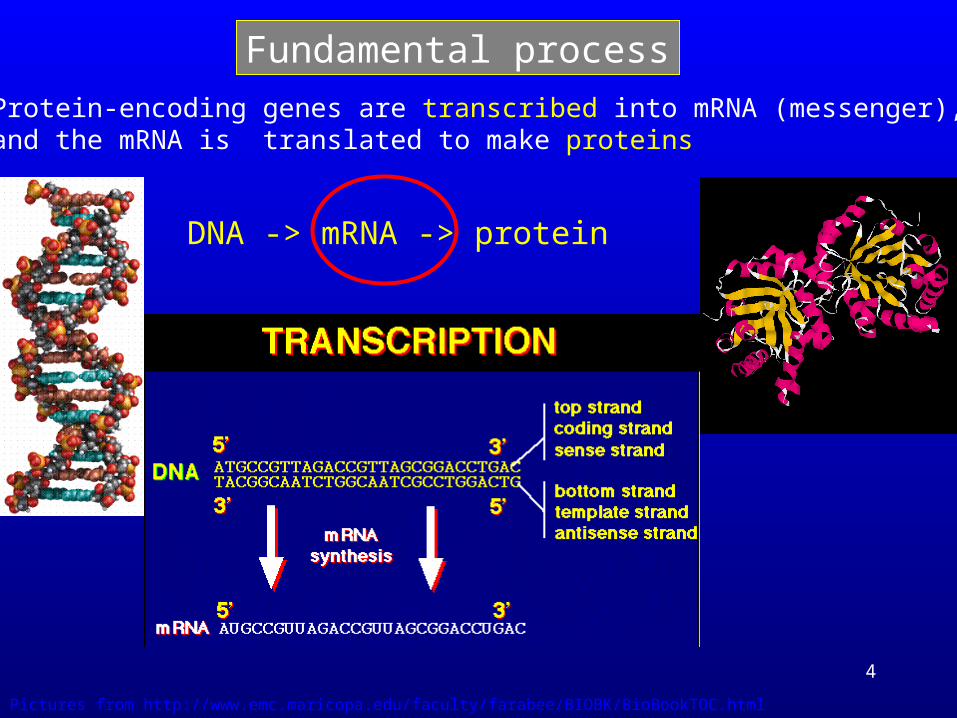
DNA -> mRNA -> protein
Pictures from http://www.emc.maricopa.edu/faculty/farabee/BIOBK/BioBookTOC.html
Protein-encoding genes are transcribed into mRNA (messenger), and the mRNA is translated to make proteins
Fundamental process

5
DNA Microarrays are used to measure the relative abundance
of mRNA, providing information on gene expression in a particular
cell, under particular conditions
The fundamental principle used to measure the expression is that of hybridisation between a sample and probes:
– Known sequences of single-stranded DNA representing genes are immobilised on microarray–Tissue sample (with unknown concentration of RNA) fluorescently labelled– Sample hybridised to array– Array scanned to measure amount of RNA present for each sequence
The expression level of ten of thousands of probes are measured on a single microarray !
gene expression profile
What are gene expression data ?
gene expression measure

6
Variation and uncertainty
• condition/treatment• biological• array manufacture• imaging• technical
• gene specific variability of the probes for a gene
• within/between array variation
Gene expression data (e.g. Affymetrix) is the result of multiple sources of variability
Structured statistical modelling allows considering all uncertainty at once

7
Example of within vs between strains gene variability
• 7 cross-bred strains of mice that differ only by a small portion of chromosome 1
• Strains have different phenotypes related to immunological disorders
• For each line, 9 animals used to obtain 3 pooled RNA extracts from spleen 7 x 3 samples
Excellent experimental design to minimise “biological variability between replicate animals”
Aim: to tease out differences between expression profiles of the 7 lines of mice and relate these to locations on chromosome 1

8
Biological variability is large !
Total variance calculatedover the 21 samples
Average (over the 7 groups) of within strain variance calculated from the 3 pooled samples
Ratio within/total
9
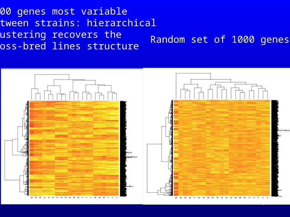
1000 genes most variablebetween strains: hierarchicalclustering recovers thecross-bred lines structure
Random set of 1000 genes

10
Common characteristics of genomics data sets• High dimensional data (ten of thousands of
genes) and few samples• Many sources of variability (low signal/noise
ratio)
Common issues
• Pre-processing and data reduction• Multiple testing• Need to borrow information• Importance to include prior biological knowledge

11
Part 2
• Introduction• A fully Bayesian gene expression index (BGX)
– Single array model– Multiple array model
• Differential expression and array effects• Mixture models• Discussion

12
A fully Bayesian Gene eXpression index for Affymetrix GeneChip arrays
Anne Mette HeinSR, Helen Causton,
Graeme Ambler, Peter Green
Background correctionGene specific variability
(probe)
PMMM
PMMM
PMMM
PMMM
Gene index BGX
Raw intensities

13
**
**
*
Slide courtesy of Affymetrix
Zoom Image of Hybridised Array
Expressed PM
Non-expressed PM
Image of Hybridised Array
Hybridised Spot
Each gene g represented by probe set: (J:11-20)
Perfect match: PMg1,…, PMgJ
Mis-match: MMg1,…, MMgJ
expression measure for gene g
Affymetrix GeneChips:

14
Commonly used methods for estimation expression levels from GeneChips
MAS5:
• uses PM and MMs. Imputes IMs from MMs to obtain all PM-MMs positive
• gene expression measure : estimate obtained by applying Tukey Biweight to the set of log(PM-MM) values in the probe set
RMA:
• uses PMs only.
• Fits an model with additive gene and probe effects to log-scale background corrected PMs using median polish
Characteristics: positive, robust, noisy at low levels
Characteristics: positive, robust, attenuated signal detection

15
Variability across conditions is conditioned by the choice of summary measure ! Beware of filtering
Mean (left) and Empirical standard deviation (right) over 7 conditions (arrays) for 45000 genes estimated by 2 different methods for quantifying gene expression
mean

16
• The intensity for the PM measurement for probe (reporter) j and gene g is due to binding
of labelled fragments that perfectly match the oligos in the spot
The true Signal Sgj
of labelled fragments that do not
perfectly match these oligos
The non-specific hybridisation Hgj
• The intensity of the corresponding MM measurement is caused
by a binding fraction Φ of the true signal Sgj
by non-specific hybridisation Hgj
Model assumptions and key biological parameters
17
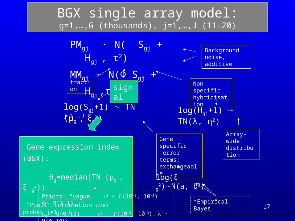
BGX single array model:g=1,…,G (thousands), j=1,…,J (11-20)
Gene specific error terms:exchangeable
log(ξ g2)N(a,
b2)
log(Sgj+1) TN (μg , ξg2)
j=1,…,J
Gene expression index (BGX):
g=median(TN (μg , ξ g2))
“Pools” information over probes j=1,…,J
log(Hgj+1) TN(λ, η2)
Array-wide distribution
PMgj N( Sgj + Hgj , τ2)
MMgj N(Φ Sgj + Hgj ,τ2) Background noise, additive
signal Non-specific hybridisation
fraction
Priors: “vague” 2 ~ (10-3, 10-3) ~ B(1,1),
g ~ U(0,15) 2 ~ (10-3, 10-3), ~ N(0,103) “Empirical Bayes”
18
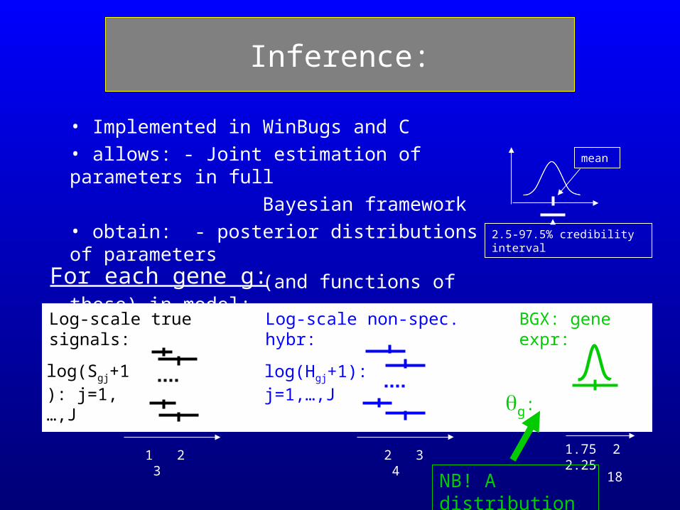
Inference:
mean
2.5-97.5% credibility interval
• Implemented in WinBugs and C• allows: - Joint estimation of parameters in full
Bayesian framework• obtain: - posterior distributions of parameters
(and functions of these) in model:
1 2 3 2 3 4 1.75 2 2.25
For each gene g:
log(Sgj+1): j=1,…,J
log(Hgj+1): j=1,…,J
g:
Log-scale true signals: Log-scale non-spec. hybr: BGX: gene expr:
NB! A distribution

19
Computational issues
• We found mixing slow for gene specific parameters (μg , ξg2)
and large autocorrelation • For low signal (bottom 25%) more variability of Sgj and Hgj ,
and less separation
So less information on (μg , ξg2) and longer runs are
needed• For the full hierarchical model, the convergence of the
hyperparameters for the distribution of ξg2 was problematic
• We studied sensitivity to a range of plausible values for those and implemented an “empirical Bayes” version of the model which was reproducible with sensible run length

20
Posterior mean of g using a runof 30 000 versus those obtainedfrom runs of 5 000, 10 000 and20 000 sweeps
Reproducibilityis obtained withshort runs forlarge expressionvalues
Longer runsare necessary for low expression values

21
• 14 samples of cRNA from acute myeloid leukemia (AML) tumor cell line
• In sample k: each of 11 genes spiked in at concentration ck:
sample k: 1 2 3 4 5 6 7 8 9 10 11 12 13 14 conc. ck(pM): 0.0 0.5 0.75 1.0 1.5 2.0 3.0 5.0 12.5 25 50 75 100 150
• Each sample hybridised to an array
Single array model performance:Data set : varying concentrations (geneLogic):
Consider subset consisting of 500 normal genes
+ 11 spike-ins

22
Single array model:examples of posterior distributions of BGX
expression indices
Each curve(truncated normal
with median param.) represents a gene
Examples with data:
o: log(PMgj-MMgj)
j=1,…,Jg
(at 0 if not defined)
Mean +- 1SD

23
Single array model performance:
11 genes spiked in at 13 (increasing)
concentrations
BGX index g increases with
concentration …..
… except for gene 7 (spiked-in??)
Indication of smooth
& sustained increase
over a wider range of
concentrations
Comparison with other expression measures
24
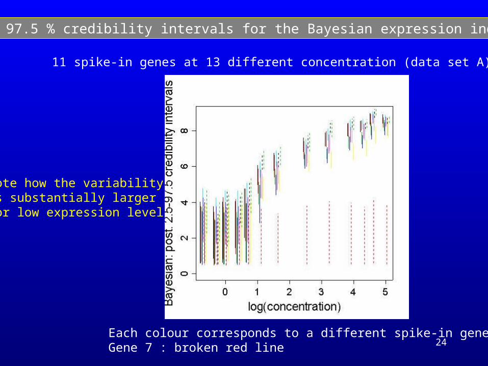
2.5 – 97.5 % credibility intervals for the Bayesian expression index
11 spike-in genes at 13 different concentration (data set A)
Note how the variabilityis substantially larger for low expression level
Each colour corresponds to a different spike-in geneGene 7 : broken red line
25
PMMM
PMMM
PMMM
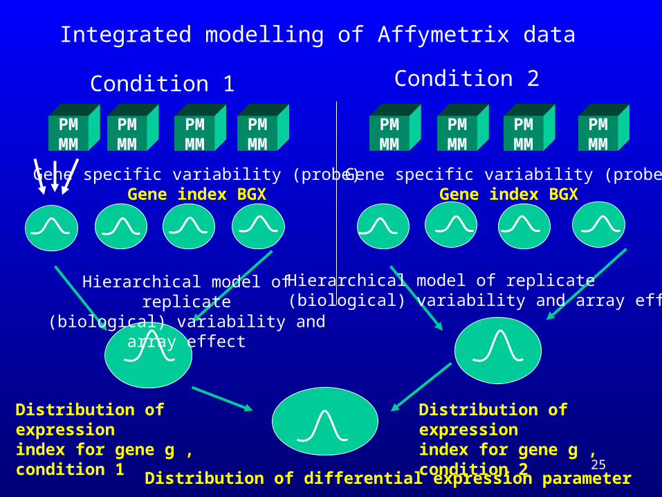
Gene specific variability (probe)Gene index BGX
Condition 1
PMMM
PMMM
PMMM
PMMM
Gene specific variability (probe)Gene index BGX
Distribution of differential expression parameter
Condition 2
Integrated modelling of Affymetrix data
PMMM
Distribution of expression index for gene g , condition 1
Distribution of expression index for gene g , condition 2
Hierarchical model of replicate(biological) variability and array effect
Hierarchical model of replicate(biological) variability and array effect

26
PMgjcr N( Sgjcr+ Hgjcr , τcr2)
MMgjcr N(ΦSgjcr+ Hgjcr , τcr2)
BGX Multiple array model: conditions: c=1,…,C, replicates: r = 1,…,Rc
log(Sgjcr+1) TN (μgc , ξ gc2)
Gene and condition specific BGX
gc=median(TN(μgc, ξ gc
2)) “Pools” information over replicate probe sets j = 1,…J, r = 1,…,Rc
Background noise, additiveArray specific
log(Hgjcr+1) TN(λcr,ηcr2)
Array-specific distribution of non-specific hybridisation

27
Subset of AffyU133A spike-in data set(AffyComp)
Consider:
• Six arrays, 1154 genes (every 20th and 42 spike-ins)
• Same cRNA hybridised to all arrays EXCEPT for spike-ins:
`1` `2` `3` … `12` `13` `14`
Spike-in genes: 1-3 4-6 7-9 … 34-36 37-39 40-42
Spike-in conc (pM):
Condition 1 (array 1-3): 0.0 0.25 0.50 … 128 256 512
Condition 2 (array 4-6): 0.25 0.50 1.00 … 256 512 0.00
Fold change: - 2 2 … 2 2 -

28
BGX: measure of uncertainty providedPosterior mean +- 1SD credibility intervals
diffg=bgxg,1- bgxg,2
}
Spike in 1113 -1154above the blue line
Blue stars show RMA measure

29
Part 3
• Introduction• A fully Bayesian gene expression index (BGX)• Differential expression and array effects
– Non linear array effects
– Model checking
• Mixture models• Discussion
30
Differential expression and array effects
Alex Lewin SR, Natalia Bochkina, Tim Aitman

31
Data Set and Biological question
Biological Question
Understand the mechanisms of insulin resistanceUsing animal models where key genes are knockout and
comparison made between gene expression of wildtype (normal) and knockout mice
Data set A (MAS 5) ( 12000 genes on each array)
3 wildtype mice compared with 3 mice with Cd36 knocked out
Data set B (RMA) ( 22700 genes on each array)
8 wildtype mice compared with 8 knocked out mice

32
Differential expression parameter
Condition 1 Condition 2
Posterior distribution
(flat prior)
Mixture modelling for classification
Hierarchical model of replicateVariability and array effect
Hierarchical model of replicateVariability and array effect
Start with given pointestimates of expression

33
Condition 1 (3 replicates)
Condition 2 (3 replicates)
Needs ‘normalisation’
Spline curves shown
Exploratory analysis of array effect
Mouse dataset A

34
Model for Differential Expression
• Expression-level-dependent normalisation
• Only few replicates per gene, so share information between genes to estimate variability of gene expression between the replicates
• To select interesting genes:– Use posterior distribution of quantities of interest,
function of, ranks ….– Use mixture prior on the differential expression
parameter

35
Data: ygsr = log gene expression for gene g, replicate r
g = gene effect
δg = differential effect for gene g between 2 conditions
r(g)s = array effect (expression-level dependent)
gs2 = gene variance
• 1st level yg1r N(g – ½ δg + r(g)1 , g1
2),
yg2r N(g + ½ δg + r(g)2 , g22),
Σrr(g)s = 0, r(g)s = function of g , parameters {a} and {b}
• 2nd level
Priors for g , δg, coefficients {a} and {b}
gs2 lognormal (μs, τs)
Bayesian hierarchical model for differential expression
36
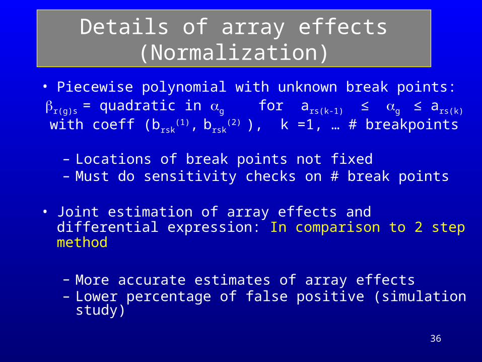
• Piecewise polynomial with unknown break points:r(g)s = quadratic in g for ars(k-1) ≤ g ≤ ars(k)
with coeff (brsk(1), brsk
(2) ), k =1, … # breakpoints
– Locations of break points not fixed– Must do sensitivity checks on # break points
• Joint estimation of array effects and differential expression: In comparison to 2 step method
– More accurate estimates of array effects– Lower percentage of false positive (simulation study)
Details of array effects (Normalization)

37
Mouse Data set A
3 replicate arrays (wildtype mouse data)
Model: posterior meansE(r(g)s | data) v. E(g | data)
Data: ygsr - E(g | data)
For this data set, cubic fits well

38
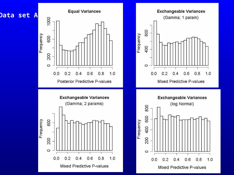
• Check assumptions on gene variances, e.g. exchangeable variances, what distribution ?
• Predict sample variance Sg2 new (a chosen checking function)
from the model specification (not using the data for this)
• Compare predicted Sg2 new with observed Sg
2 obs
‘Bayesian p-value’: Prob( Sg2 new > Sg
2 obs )
• Distribution of p-values approx Uniform if model is ‘true’
(Marshall and Spiegelhalter, 2003)• Easily implemented in MCMC algorithm
Bayesian Model Checking
39
Data set A

40
Possible Statistics for Differential Expression
δg ≈ log fold change
δg* = δg / (σ2 g1 / R1 + σ2 g2 / R2 )½ (standardised difference)
• We obtain the posterior distribution of all {δg} and/or
{δg* }
• Can compute directly posterior probability of genes satisfying criterion X of interest:
pg,X = Prob( g of “interest” | Criterion X, data)
• Can compute the distributions of ranks

41
Gene is of interest if |log fold change| > log(2) and log (overall expression) > 4
Criterion X
The majority of the genes
have very small pg,X :
90% of genes
have pg,X < 0.2
Genes withpg,X > 0.5 (green)
# 280pg,X > 0.8 (red)
# 46
pg,X = 0.49
Plot of log fold change versus overall expression level
Data set A 3 wildtype mice compared to 3 knockout mice (U74A chip) Mas5
Genes with low overall expression have a greater range of fold change than those with higher expression

42
Gene is of interest if |log fold change| > log (1.5)Criterion X:
The majority of the genes
have very small pg,X :
97% of genes
have pg,X < 0.2
Genes withpg,X > 0.5 (green)
# 292pg,X > 0.8 (red)
# 139
Plot of log fold change versus overall expression level
Experiment: 8 wildtype mice compared to 8 knockout mice RMA

43
Posterior probabilities and log fold change
Data set A : 3 replicates MAS5 Data set B : 8 replicates RMA

44
Credibility intervals for ranks
100 genes with lowest rank (most under/over expressed)
Low rank, high uncertainty
Low rank, low uncertainty
Data set B

45
• Compute
Probability ( | δg* | > 2 | data)
Bayesian analogue of a t test !• Order genes
• Select genes such that
Using the posterior distribution of δg*
(standardised difference)
Probability ( | δg* | > 2 | data) > cut-off ( in blue)
By comparison, additional genes selected by a standard
T test with p value < 5% are in red)

46
Part 4
• Introduction• A fully Bayesian gene expression index • Differential expression and array effects• Mixture models
– Classification for differential expression– Bayesian estimate of False Discovery Rates– CGH arrays: models including information on clones spatial location on
chromosome
• Discussion

47
Mixture and Bayesian estimation of false discovery rates
Natalia Bochkina, Philippe Broët Alex Lewin, SR

48
• Gene lists can be built by computing separately a criteria for each gene and ranking
• Thousands of genes are considered simultaneously• How to assess the performance of such lists ?
Multiple Testing Problem
Statistical ChallengeSelect interesting genes without including too many false
positives in a gene list
A gene is a false positive if it is included in the list when it is truly unmodified under the experimental set up
Want an evaluation of the expected false discovery rate (FDR)

49
Bayesian Estimate of FDR
• Step 1: Choose a gene specific parameter (e.g. δg ) or a gene statistic
• Step 2: Model its prior (resp marginal) distribution using a mixture model
-- with one component to model the unaffected genes (null hypothesis) e.g. point mass at 0 for δg
-- other components to model (flexibly) the alternative
• Step 3: Calculate the posterior probability for any gene of belonging to the unmodified component : pg0 | data
• Step 4: Evaluate FDR (and FNR) for any listassuming that all the gene classification are independent(Broët et al 2004) :
Bayes FDR (list) | data = 1/card(list) Σg list pg0

50
Mixture framework for differential expression
• To obtain a gene list, a commonly used method
(cf Lönnstedt & Speed 2002, Newton 2003, Smyth 2003,
…) is to define a mixture prior for δg :
• H0 δg = 0 point mass at 0 with probability p0
• H1 δg ~ flexible 2-sided distribution to model pattern of differential expression
Classify each gene following its posterior probabilities of not being in the null: 1- pg0
Use Bayes rule or fix the FDR to get a cutoff

51
Mixture prior for differential expression
• In full Bayesian framework, introduce latent allocation variable zg to help computations
• Joint estimation of all the mixture parameters (including p0) avoids plugging-in of values (e.g. p0) that are influential on the classification
• Sensitivity to prior settings of the alternative distribution
• Performance has been tested on simulated data sets
Poster by Natalia Bochkina

52
Performance of the mixture prior
yg1r = g - ½ δg + g1r , r = 1, … R1
yg2r = g + ½ δg + g2r , r = 1, … R2
(For simplification, we assume that the data has been pre normalised)
Var(gsr ) = σ2gs ~ IG(as, bs)
δg ~ p0δ0 + p1G (1.5, 1) + p2G (1.5, 2)
H0 H1
Dirichlet distribution for (p0, p1, p2)
Exponential hyper prior for 1 and 2

53
Estimation
• Estimation of all parameters combines information from biological replicates and between condition contrasts
• s2gs = 1/Rs Σr (ygsr - ygs. )2 , s = 1,2
Within condition biological variability
• 1/Rs Σr ygsr = ygs. ,
Average expression over replicates
• ½(yg1.+ yg2.) Average expression over conditions
• ½(yg1.- yg2.) Between conditions contrast
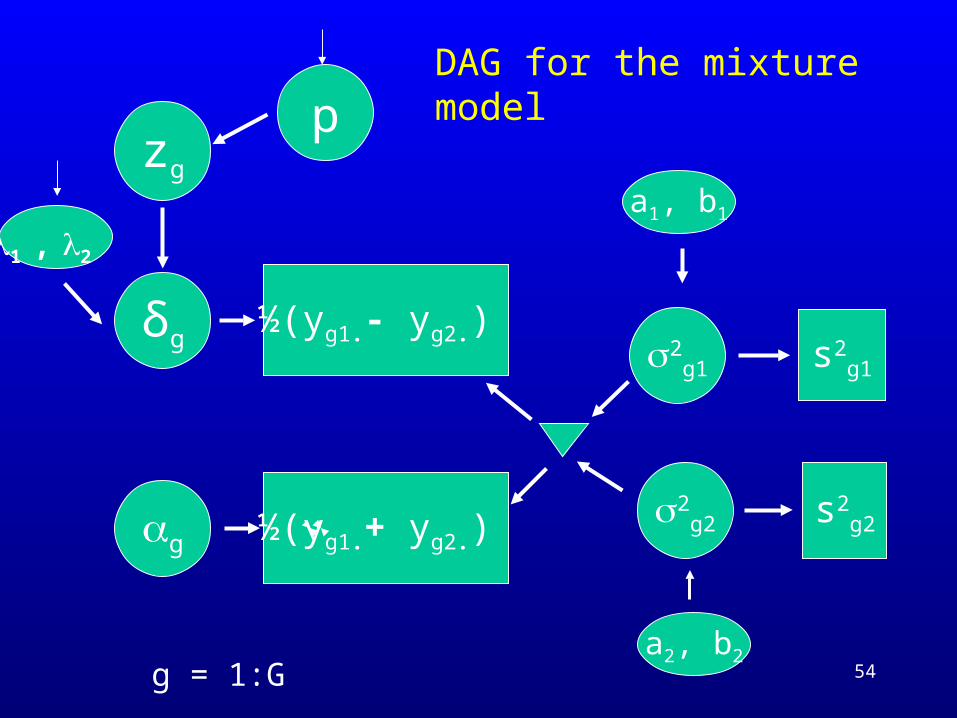
54g = 1:G
DAG for the mixture model
a1, b1
½(yg1.+ yg2.)
1 , 2
δg 2g1 s2
g1
2g2 s2
g2g
zg
a2, b2
p
½(yg1.- yg2.)

55
Simulated data
ygr ~ N(δg , σ2g) (8 replicates)
σ2gs ~ IG(1.5, 0.05)
δg ~ (-1)Bern(0.5) G(2,2), g=1:200
δg = 0, g=201:1000
Choice of simulation parametersinspired by estimates found in analyses of biological data sets
Plot of the true differences

56Post Prob (g H1) = 1- pg0
Bayesrule
FDR (black)FNR (blue)as a function of1- pg0
Observedand estimatedFDR/FNRcorrespond well
Important feature
57
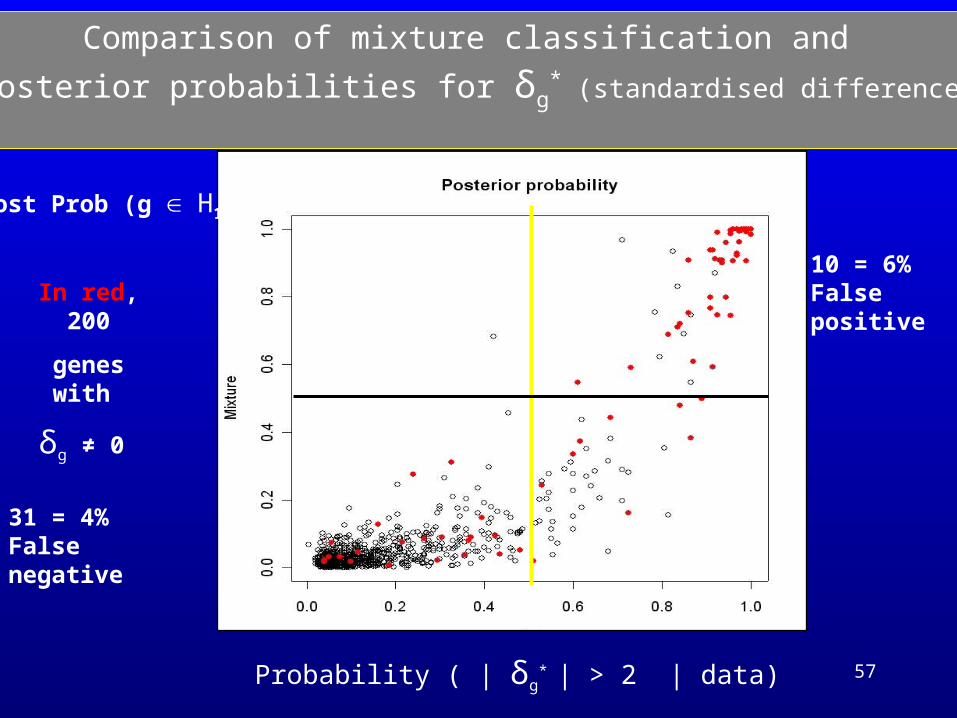
Comparison of mixture classification and
posterior probabilities for δg* (standardised differences)
In red, 200
genes with
δg ≠ 0
Probability ( | δg* | > 2 | data)
31 = 4%False negative
10 = 6%False positive
Post Prob (g H1)

58
Wrongly classified by mixture:
truly dif. expressed,
truly not dif. expressed
Classification errorsare on the borderline:
Confusion betweensize of fold change and biological variability

59
Another simulation
Can we improve estimationof within conditionbiological variability ?
2628 data points
Many points addedon borderline:classificationerrors in red

60g = 1:G
DAG for the mixture model
a1, b1
½(yg1.+ yg2.)
1 , 2
δg 2g1 s2
g1
2g2 s2
g2g
zg
a2, b2
p
½(yg1.- yg2.)
The varianceestimates areinfluenced bythe mixtureparameters
Use only partialinformation fromthe replicatesto estimate2
gs and feed
forwardin the mixture ?

61
Mixture, full vs partial
In 46 data pointswith improvedclassification when‘feed back frommixture is cut’
In11 data pointswith changedbut new incorrect classification
Classificationaltered for 57 points:
Work in progress

62
Mixture models in CGH arrays experiments
• Philippe Broët, SR
• Curie Institute oncology department
CGH = Competitive Genomic Hybridization
between fluorescein- labelled normal and pathologic
samples to an array containing clones designed
to cover certain areas of the genome

63
In oncology, where carcinogenesis is associated with complex chromosomic alterations, CGH array can be used for detailed analysis of genomic changes in copy number (gains or loss of genetic information) in the tumor sample.
Amplification of an oncogene or deletion of a tumor suppressor gene are considered as important mechanisms for tumorigenesis
Loss Gain
Tumor supressor gene Oncogene
Aim: study genomic alterations

64
Specificity of CGH array experiment
A priori biological knowledge from conventional CGH :• Limited number of states for a sequence :
- presence, - deletion, - gain(s)
corresponding to different intensity ratios on the slide
Mixture model to capture the underlying discrete states
• Clones located contiguously on chromosomes are likely to carry alterations of the same type
Use clone spatial location in the allocation model
• Some CGH custom array experiments target
restricted areas of the genome Large proportion of genomic alterations are expected

65
3 component mixture model with spatial allocation
ygr N(θg , g2) , normal versus tumoral change, clone g
replicate measure r
θg wg0N(μ0 ,02) + wg1N(μ1 ,1
2) + wg2N(μ2 ,22)
μ0 : known central estimate obtained from reference clonesIntroduce centred spatial autoregressive Markov random fields, {ug
0}, {ug1}, {ug
2} with nearest neighbours along the chromosomes
presence
deletion gain
x x xg -1 g g+1
Spatial neighbours of g
Define mixture proportions to depend on the chromosomic location
via a logistic model: wgk = exp(ugk) / Σm exp(ug
m)
favours allocation of nearby clones to same componentWork in progress
66
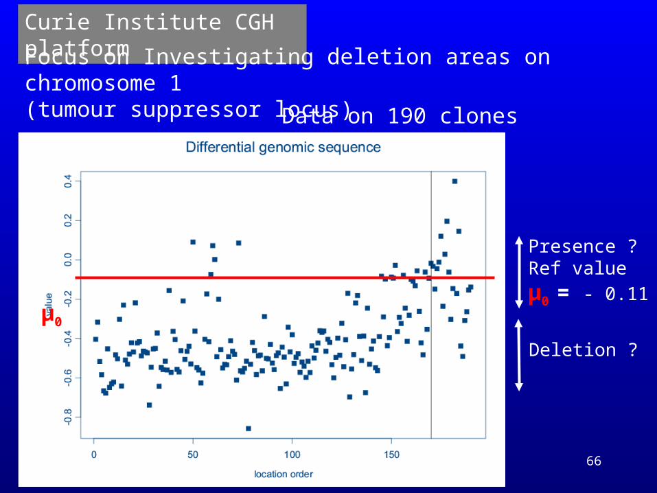
Deletion ?
Presence ?Ref value
μ0 = - 0.11μ0
Curie Institute CGH platform
Focus on Investigating deletion areas on chromosome 1 (tumour suppressor locus)
Data on 190 clones

67
Mixture model posteriorprobability p of clone being deleted
Classification withcut-off at p ≥ 0.8
Short arm

68
Bayesian gene expression measure (BGX)
Good range of resolution, provides credibility intervals
Differential Expression
Expression-level-dependent normalisationBorrow information across genes for variance estimationGene lists based on posterior probabilities or mixture classification
False Discovery Rate
Mixture gives good estimate of FDR and classifiesFlexibility to incorporate a priori biological features, e.g. dependence on chromosomic location
Future work Mixture prior on BGX index, with uncertainty propagated to mixture parameters, comparison of marginal and prior mixture approaches, clustering of profiles for more general experimental set-ups
Summary

69
Papers and technical reports:
Hein AM., Richardson S., Causton H., Ambler G. and Green P. (2004)BGX: a fully Bayesian gene expression index for Affymetrix GeneChip data
(to appear in Biostatistics)
Lewin A., Richardson S., Marshall C., Glazier A. and Aitman T. (2003) Bayesian Modelling of Differential Gene Expression
(under revision for Biometrics)
Broët P., Lewin A., Richardson S., Dalmasso C. and Magdelenat H. (2004) A mixture model-based strategy for selecting sets of genes in multiclass response microarray experiments. Bioinformatics 22, 2562-2571.
Broët, P., Richardson, S. and Radvanyi, F. (2002) Bayesian Hierarchical Model for Identifying Changes in Gene Expression from Microarray Experiments. Journal of Computational Biology 9, 671-683.
Available athttp ://www.bgx.org.uk/
Thanks