S.Y.B Tech Sub:- INDEX Sr Page DOP DOS Marks No. (10 ...
30
1 Terna Public Charitable Trust’s College of Engineering, Osmanabad Dept. of Civil Engineering Class:- S.Y.B Tech Sub:- Hydraulics-II INDEX Sr No. Name of Experiment Page No. DOP DOS Marks (10) Sign Remark Group A (any Three) 01 Calibration of V notch / Rectangular notch 02 Calibration of Ogee Weir 03 Study of hydraulic jump a) Verification of sequent depths, b) Determination of loss in jump 04 Study of flow below gates – Discharge v/s head relation, Equation of flow, Determination of contraction in fluid in downstream of gate 05 Velocity distribution in open channel in transverse direction of flow Group B (any Three) 06 Impact of jet 07 Study of Turbines (Demonstration) 08 Tests on Centrifugal Pump 09 Study of Charts for Selection of Pumps
Transcript of S.Y.B Tech Sub:- INDEX Sr Page DOP DOS Marks No. (10 ...

1
Terna Public Charitable Trust’s
College of Engineering, Osmanabad
Dept. of Civil Engineering
Class:- S.Y.B Tech Sub:- Hydraulics-II
INDEX
Sr
No.
Name of Experiment
Page
No.
DOP DOS Marks
(10)
Sign Remark
Group A (any Three) 01 Calibration of V notch /
Rectangular notch
02 Calibration of Ogee Weir 03 Study of hydraulic jump
a) Verification of sequent
depths,
b) Determination of loss in
jump
04 Study of flow below gates –
Discharge v/s head relation,
Equation of flow,
Determination of contraction in
fluid in downstream of gate
05 Velocity distribution in open
channel in transverse direction
of flow
Group B (any Three) 06 Impact of jet 07 Study of Turbines
(Demonstration)
08 Tests on Centrifugal Pump 09 Study of Charts for Selection of
Pumps
2
Experiment No. : 01
Measurement of discharge Aim: - To determine the co-efficient of discharge of a rectangular notch.
Theory:-
Notch: Notch is a device or arrangement made across the flow in open channel for measuring
the discharge.
The discharge coefficient Cd of a rectangular notch must be determined by applying formula
√
Fig.1 Rectangular Notch Apparatus Setup
Experimental Procedure:-
1. Check the experimental setup for leaks. Measure the dimensions of collecting tank
and the notch.
2. Observe the initial reading of the hook gauge and make sure there is no discharge.
Note down the sill level position of the hook gauge.
3. Open the inlet valve of the supply pipe for a slightly increased discharge. Wait for
sometime till the flow become steady.
4. Adjust the hook gauge to touch the new water level and note down the reading.
Difference of this hook gauge reading with initial still level reading is the head
over the notch (h).
5. Collect the water in the collecting tank and observe the time t to collect R

3
Raise/Height of water.
6. Repeat the above procedure for different flow rates by adjusting the inlet valve
opening and tabulate the readings.
7. Complete the tabulation and find the mean value of CD.
8. Draw the necessary graphs and calibrate the notch.
Observations:-
Initial Hook gauge reading = mm
Observation Table
Sl.No. Sill level
reading
mm
Reading
of head
over the
sill
Mm
Head
over
the sill
h
cm
Rise
cm
Time
taken
t
sec.
Q t h
m3/s
Q act
m3/s
Coefficient
of
discharge
C d
Specimen Calculations:-
Q a = A.R/t
where A = 6400 cm2
Q a = C d Q t h
Q t h = (2/3) L √(2g) h3/2
g = Acceleration due to gravity = 9.81 m/sec2
C d = Q a/Q t
Results:-
Coefficient of discharge of the given triangular notch from
1.Calculations
Conclusion:-
Average Cd _____________

4
Experiment No. : 02
Calibration of Ogee Weir
Aim : To calibrate the ogee weir and hence to determine the value of Cd
Apparatus :
1. A constant steady water supply with a means of varying the flow
2. An approach channel (flume)
3. ogee weir (to be calibrated)
4. A flow rate measuring facility ((calibrated rectangular notch)
5. Hook gauge
Theory:
Generally ogee shaped weirs are provided for the spillway of a storage dam. The crest of
the ogee weir is slightly rises and falls into parabolic form. Flow over ogee weir is also
similar to flow over rectangular weir. The crest of the weir rises upto a maximum of
0.115H, where H is the head over the weir.
Formula governing the flow over a ogee weir is Q = = (2/3)LCd √2 H3/2 -----------1
Where L= length of weir (measured perpendicular to the direction of flow or the width of
the channel in the laboratory)
Procedure:
1. Start the pump with the help of electrical 3phase DOL starter (Direct on line) and
observe water flowing in the flume. Wait till the water level rises to the crest level
of the weir fixed at the down stream end.
2. Adjust the vernier scale any whole number of main scale division and lock it.
3. Bring the hook gauge point exactly to the water level, note it as initial level h1
4. measure the discharge flowing over the ogee weir note it as h2
5. Procedure was repeated for different discharges.

5
Observation & calculation
Head over weir Length of weir
Sr
No
Rotameter
Reading
LPM
Crest
Level
h1m
Water
Level
h2m
Head over weir
H = h1- h2
Q act
m3/sec
Q th
m3/sec
Cd
Calculations:(any one trial)
Qth =(2/3) √2 LH3/2
Qact = Rotameter reading in m3 / sec
Cd= Qact / Qth
Graphically,
A log Qa vs log H suggests a straight line relation as shown in fig. This equation is of the
form
Qa=(2/3) √2 Cd L x H3/2
=KHn
Taking log on both sides
log Qa =logK+n logH
Where logK is the intercept on the log Q axis n is the slope of the straight line. n
Knowing the valve of logK, K can be determined and then the value of Cd is determined as
follows. 1
Cd = (1/K ) X (1/Slope)
6
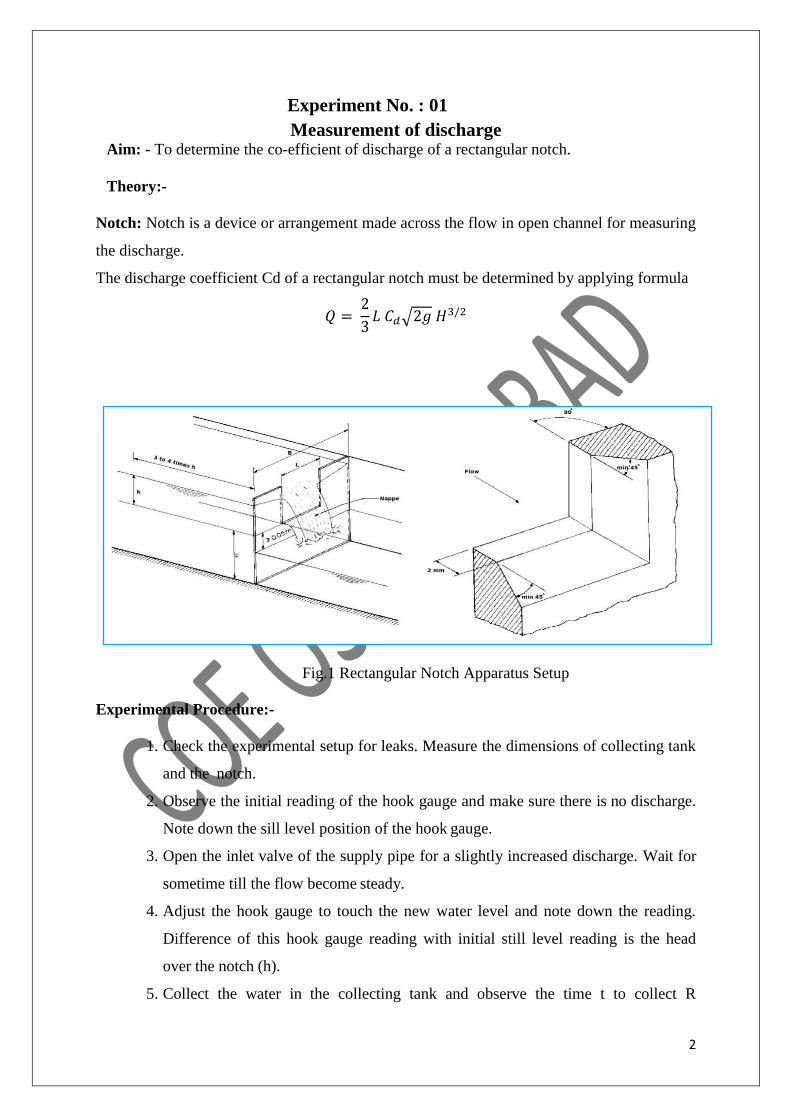
Experiment no 3 (a)
Study of hydraulic jump
Aim: To determine Hydraulic jump .
Experimental Setup:
For conducting this experiment long hollow rectangular channel is used with bed
slope adjustments. Inlet pipe is provided with flow regulating arrangement. Outlet of
channel is directly taken to the measuring tank which is provided with piezometer
tube arrangement outlet is provided with measuring tank
Theory
The rise of water level, which takes place due to transformation, the unstable
shooting flow (super critical) to the stable streaming flow (sub critical flow).
The height of water of the section 1-1 is small. As we move towards downstream,
the height or depth of water increases rapidly over a short length of the channel. This is
because of the section 1-1, the flow is a shooting flow as the depth of water at section 1-1
is less than critical depth. Shooting flow is an unstable type of flow & does not continue
on the downstream side then this shooting flow will convert itself into a streaming flow
& hence depth of water will increase.
Hydraulic jumps are very efficient in dissipating the energy of the flow to make it
more controllable & les erosive. In engineering practice, the hydraulic jump
frequently appears downstream from overflow structures (spillways), or under flow
structures (slvice gates), where velocities are height.
A hydraulic jump is formed when liquid at high velocity discharges into a zone
of lower velocity only if the 3 independent velocities (y1, y2, fr1) of the hydraulic
jump equation conform to the following equation:
Y2 = y1/2 [-1+√1+8Fr2 ]

7
Use of Hydraulic jump:
Hydraulic jump is used to dissipate or destroy the energy of water where it is not
needed otherwise it may cause damage to hydraulic structures.
It may be used for mixing of certain chemicals like in case of water treatment
plants.
It may also be used as a discharge measuring device.
Procedure:
1. start the pump to supply water to the flume.
2. Then close the tail gate to allow water to accumulate and to develop hydraulic
jump.
3. adjusted the position of the hydraulic jump by adjusting the amount of closure of
slvice gate.
4. then measured the depth of the bed of flume by using a point gauge.
5. Measure depth of water befor jump.
6. Measure depth of water after jump
7. Find length of jump and specific energy loss.
Observations:
1. Width of channel “ B ”= cm
2. Length of channel= m
8
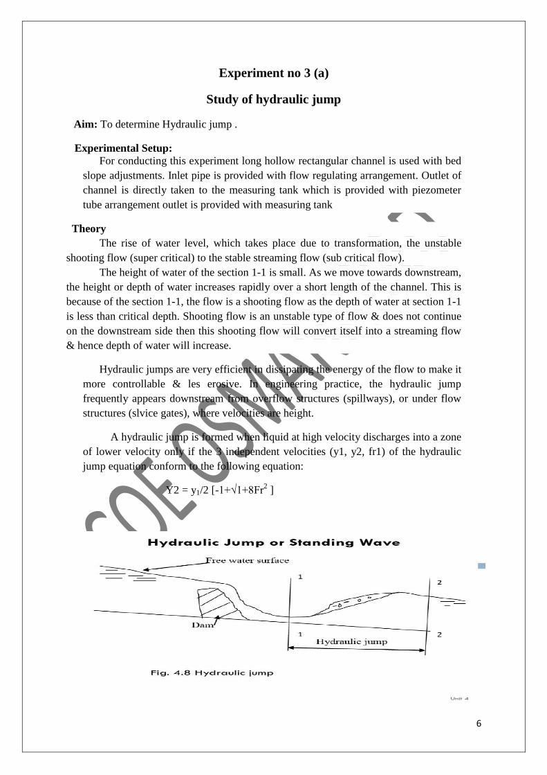
Experiment no 3 (b)
Aim:_
To determine sequent depth & energy loss due to hydraulic jump.
Apparatus:-
Hydraulic lifting flume with spillway model point gauge mounted on trolley a shutter to
control flow discharge measurement tank with piezometer, scale, stopwatch.
Theory:-
i) Hydraulic Jump:- If the sub critical flow changes its state of flow into super vertical flow in
a short length is called as hydraulic jump
ii)How expressions for hydraulic jump.
iii) Types of hydraulic jump.
v) length or height of hydraulic jump.
Procedure:- i) Measure the length of channel dimensions of measuring tank.
ii) Keep upstream take open & open inlet valve.
iii)Allow the water to flow through flume control upstream sluice gate so as to createsuper
critical flow.
iv)Control the down-stream sluice gate to createahydraulic jump.at the top of weir.
v)When the jump becomes stationary measure the initial depth &sequent depth or length o
fhydraulic jump.
vi) At the same time measure the discharge with the help of measuring tank & pyrometer i.e.
ΔH&Δt
Observations :

9
1. Width of channel = m
2. Area of tank = m2
Observation table
Sr
no
Initial depth
before jump
Discharge
after
jump
Discharge
Qact= Δ H xA
Δt
V1=
Qact/
(b x
y1)
(m/s)
V2 =
Qact/
(b x
y2)
(m/s)
Fr
=
V1/
y2 =
Y1/2
)
(Y2-
y1)
Heigh
t Of
Hydra
ulic
Jump
Length
of
Hydr
aulic
Jump is
(Y2- Y1)
Loss of
energy due to
hydraulic
Jump =
( y2 y1)3
/
(4 x Y1 xY2) IR FR Y 1 IR F
R
Y
2
ΔH
(m)
ΔT
(Sec
)
Qact
m3/Sec)
1
2
3
4
5
Sample Calculations:-
i)Qact = (ΔH x A )/ Δt = (0.1 x 0.64)/25 = 2.56 x 10⁻³
m3/sec
ii) v1 = Qact/A = 2.568 x 10⁻³
/(0.25 x 0.018) =1.024 m/s
ii)V2 = Qact/A = 2.56 x 10 -3
/ (0.25 x 0.03) = 0.341 m/
iii)Froude no. Fr = V1/√ = 1.024/(
Fr= 3.26
iv) Y2= Y1/2 ( ) – 1)
=0.01/2 ) – 1)
Y2 = 0.041
v) Height of hydraulic Jump = Y2– Y1
= 0.03- 0.0 1
= 0.02m
Vi) length of hydraulic Jump = 5.5.( Y2 - Y1 )
= 5.5 ( 0.03- 0.0 1)
L J = 0.11m

10
7) Loss of energy due to hydraulic jump
ΔL =( Y2–Y1)3 / (4 x Y1 x Y2)
= ( 0.03–0.01)3 / (4 x 0.03 x 0.01)
ΔE = 6.66 x 10⁻³
Kg-m/kg.
Results
Sequent depth = Y2 – Y1 = m
The loss of energy clue to hydraulic jump =ΔF= kg.m/kg.

11
Experiment No 04
SLUICE GATE EXPERIMENT
Open Channel Flow
Pressure at water surface is atmospheric or zero gage pressure
Water surface = piezometric head level
i.e., level registered by manometer with a piezometric tap
Open channel flow, in general, has two possible flow depths for each energy level Subcritical
and supercritical. Sluice gate changes flow from subcritical to supercritical
Flow under sluice gate
Minimum cross-sectional area (vena contracta) is slightly downstream from the gate
Ideal Flow Theory (No Energy Losses)
Q = V1*A1 = V2*A2
Experimental Studies
Discharge coefficient
Flow is never really “ideal” Coefficient is related to relative size of gate opening
Brater & King summarize some of these
General form Q = C*A*(2g*dH)0.5
Specific Energy
Energy in an open channel measured relative to the channel bottom E = y + V2/2g
For two values of y with the same value of E
E = y1 + V12 /2g = y2 + V22 /2g
Combine this with the continuity equation,
V1*b*y1 = V2*b*y2
Now we can eliminate one of the velocities and compute the other velocity without using Q.
This gives some experimental data for a two-dimensional plot of specific energy to compare
with the theoretical equation. To use the specific energy plot, we measure y2 at the vena
contracta.
As an aside, the specific energy function,
E = y + Q2 /2g*b2 y2
is actually cubic in y
i.e., -y3 + E*y2 = Q2 /2g b2
The subcritical and supercritical flows are two of the three areas for the solution. The third
area of the solution has a negative value of y, which is meaningless for open channel flow

12
Sluice Gate Experiment
Study the application of one-dimensional flow analysis involving continuity, energy and
momentum equations to a sluice gate in a rectangular channel
Flow Under A Sluice Gate
As stated earlier, there are two flow depths, subcritical and supercritical, for each energy
level.The easiest approach is to compare the measured values of y2 with values computed for
observed y1.
Force By Momentum Equation
Fx = γ* Vx *Q becomes
Fg = γ*[Q*(V1 -V2) + 0.5*b* (y12-y2
2)]
where γ = density of water
g (in the drawing) = gravity constant
Q = flow rate

13
v1, y1 = upstream velocity and depth
v2, y2 = downstream velocity and depth
b = width of rectangular channel
Force By Hydrostatic Model & By Direct Measurement
Linear hydrostatic pressure uses the simple triangular pattern of pressure, with the average
pressure at the center point times the area. (In our experiment, the top pressure is
atmospheric, which we use as H1 of zero.)
Direct measurement uses pressure measured at several points along the gate. The key is to
select the area you associate with each pressure value.
Sluice Gate Experiment: Preparation
Objectives (Presented above)
Apparatus (Same flume & measurement taps as for Weir Experiment, except tap on the sluice
gate)

14
Set up experiment:
Open surge tank valve. Open both the head and the tail (sluice) gates of the half-meter open
channel unit
Determine the longitudinal profile along the centerline of the floor of the flume to get point
gage zeros. (If not clear from a prior experiment.)
Remove air from all manometric tubing. Locate the pressure taps in the gate and on the floor
of the flume and match them to the manometer columns.
Close the drain valve, start the large pump, and open the intake valve.
Experimental data collection
Measure the profile and the sluice gate variables.
Establish a steady flow in the flume
Lower the upstream sluice gate until it impinges on the flow.
Slowly lower the gate until the flume is nearly full.
Wait for the flow to reach the steady state.
[Note: remove air from the manometer tubes A-F.]
Record the flow depths of the water surfaces both upstream and downstream of the gate. For
the supercritical section, you are trying to measure at the vena contracta.
Repeat step d until you have at least 6 measurements of depth
Measure the water surface profile & taps A-F
Close the sluice gate enough to raise level above taps A-F
Measure the depth of the water to about half-way down the channel
Also record the levels at taps A-F
Shut off the flow. Turn off the pump, close the intake valve, & open the drain valve on the
head tank.

15
Sluice gate experiment: Results
Attach your data sheet and sketch of the experimental set-up
Flow Through Sluice Gate
Using the continuity equation between the upstream and downstream flows (latter at the vena
contracta) compute the velocities on both sides of the gate for each pair of flow depths.
From Q = ViAi
V1 = Q/(b*y1) and V2 = Q/(b*y2)
Compare the specific energy (Ei = yi + Vi2 /2g) plot for the observed depths and computed
velocities with the theoretical plot at the same flow rate, Q
Compare the measured contraction coefficient with any hydraulic literature reference.
Flow Rate Calculation
Using your depth measurements upstream of the gate and at the vena contracta, along with
the continuity and energy equations, compute the flow rate and compare it with the rate given
by the flow meter
Q = V1*A1 = V2*A2
Ei = yi + Vi2 /2g
or y1 + V12 /2g = y2 + V22 /2g
Combining these: Q = 2g*b* y1* y2 / (y1 + y2)0.5
Force On Gate
Compute the force on the gate using (a) the measured pressures, (b) hydrostatic assumption,
and (c) the momentum equation.
Compare the three values in terms of accuracy and convenience.
Plot the pressure distributions on the upstream side of the sluice gate from the measured
pressures and from the hydrostatic assumption on the same chart and compare the two
patterns.

16
Experiment no 05
Velocity distribution in open channel
Aim-
To study Velocity distribution in open channel in traverse direction of flow.
Theory :-
The presence of corners & boundaries in an open channel causes the velocity vectors
of the flow to hare components not only in the longitudinal & lateral direction but also in
normal direction to the flow in a micro analysis, one is concerned only with the major
component viz, the longitudinal component „ Vx‟ The other two components being small ore
ignored &„Vx „ is designed as „V‟ The distribution of „ V „ in a channel is dependent
on the geometry of the channel .
Fig:- a Shows isolves ( contours of equal Velocity ) of „ V ‟ for a natural &
rectangular channel resp. The influence of the channel geometry is apparent. The velocity
„V‟ is zero at the solid boundaries&gradually increases with distance from the boundary. The
maximumvelocity of the cross section occurs at a certain distance below the free surface.
This dip of the maximum velocity point, giving surface velocities which. Are less than the
maximumvelocity , is due to secondary currents & is a function of the aspect ratio ( ratio of
depth to with) of the channel. Thus for a deep narrow channel the location of a
maximumvelocity point will he much lower from the water surface than for a wider channel
of the same depth This characteristic location of the maximum velocity point below the
surface has nothing to do with the wind shear on the free surface.
Fig a.
17
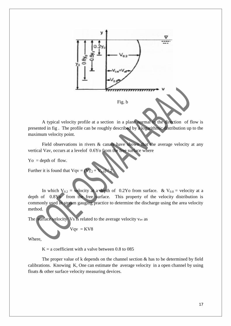
Fig. b
A typical velocity profile at a section in a plane normal to the direction of flow is
presented in fig . The profile can be roughly described by a logarithmic distribution up to the
maximum velocity point.
Field observations in rivers & canals have shown that the average velocity at any
vertical Vav, occurs at a levelof 0.6Yo from the free surface where
Yo = depth of flow.
Further it is found that Vqv = (V0.2 + Vo.8) / 2
In which V0.2 = velocity at a depth of 0.2Yo from surface. & V0.8 = velocity at a
depth of 0.8Yo from the free surface. This property of the velocity distribution is
commonly used in stream gauging practice to determine the discharge using the area velocity
method.
The surface velocity Vs is related to the average velocity vav as
Vqv = KV8
Where,
K = a coefficient with a valve between 0.8 to 085
The proper value of k depends on the channel section & has to be determined by field
calibrations. Knowing K, One can estimate the average velocity in a open channel by using
floats & other surface velocity measuring devices.

18
EXPERIMENT NO 6
IMPACT OF JET ON VANES
AIM: To determine the Co-efficient of impact jet – vanes combination by the force for
stationary vanes of different shapes VIZ: Hemispherical, Flat plate, inclined plate.
Theory:
When jet of water is directed to hit the vane of particular shape, the force is
exerted on it by fluid in the opposite direction. The amount of force exerted depends on
the diameter of jet, shape of vane, fluid density, and flow rate of water. More importantly,
it also depends on whether the vane is moving or stationary. In our case, we are concern
about the force exerted on stationary vanes. The following are the figures and formulae
for different shapes of vane, based on flow rate.
HEMISPHERICAL Ft = 2 ρ A V2/g
FLAT PLATE Ft = ρ A V2/g
INCLINED PLATE Ft = (ρ A V2/g) sin2θ
Where,
g = 9.81m/sec2
A = Area of jet in m2
ρ = Density of water = 1000 Kg/m3
V = Velocity of jet in m/sec=Q/A
θ = Angle of deflected vanes makes with the axis of striking jet, 45 degree.
Ft = theoretical force acting parallel to the direction of jet
Fa = Actual force acting parallel to the direction of jet
Description:
It is a closed circuit water re-circulating system consisting of sump tank,
mono block pump set, and jet / vane chamber. The water is drawn from sump to mono
block pump and delivers it vertically to the nozzle. The flow control valve is also
provided for controlling the water into the nozzle. The water issued out of nozzle as jet.
The jet is made to strike the vane, the force of which is transferred directly to the vane. A
collecting tank with piezo meter to measure discharge. The provision is made to change
the size of nozzle/jet and vane of different shapes.
Specifications:
Vane shapes : Flat, Hemispherical, Inclined (standard) & any other optional
shapes at extra cost.
Jets diameter : 6mm.
Measurements: Pressure of jet by pressure gauges and discharge by collecting
tank with the help of stop watch
Pump : 1 hp, single phase, 230volt with starter
Type : Recirculating with sump & jet chamber made of stainless steel.
Jet chamber : Fixed with toughened glass windows with leak proof rubber
gaskets.
OPERATION:
1. Fix the required diameter jet and the vane of required shape in position.
2. Keep the delivery valve closed & switch ON the pump.

19
3. Close the front transparent cover tightly.
4. Open the delivery valve and adjust the flow rate of water by gate wall provided.
5. Note down the diameter of jet, shape of vane, flow rate & force and tabulate the
results.
6. This way take readings for 1) different flow rates
2) Different vanes
observation table :-
Sr
no
Type of
Vane used
Time taken
for 10 cm rise
of water in
sec
Qact
M3/sec
Velocity
Of jet
m/s
Va
Actual
force
Fa
Theoretical
Force
Ft
Coefficient
Of impact
Calculation :
1. Area of the vane A=……………..m2
2. Volume of water collected U =…………m3
3. Actual discharge Qa= U/t =……………… m3/sec
4. Velocity of water jet = Va = Qa/A =………. m/s
5. Theoretical force = Ft ………..m/sec
6. Actual force Fa = ……..
7. Co-efficient of impact = k = Fa/Ft =………..
Results: Coefficient of Impact for flat vane:
Coefficient of Impact for Inclined vane:
Coefficient of Impact for curved vane:
20
EXPERIMENT NO 07
Study of turbines
Aim :- Trial On Pelton Wheel turbine.
Appratus : -
1. Pelton Wheel Turbine 2. Nozzle & Spear Arrangement
3. Pressure Gauges (03 Nos. – Range = 00 – 07 kg/cm2)
THEORY :-
Hydraulic Energy is now widely used in the world as it is one of cheap sources of
power. To convert this power into mechanical energy, turbines are used,which drive the
generators coupled to them.There are many types of turbines,i.e. Francis, Kaplan, Pelton
wheel… etc. Among these turbines Elton wheel turbin is only type being mostly used these
days. It is also called as free jet turbine and operates under a high head of water and therefore
requires a comparatively less quantity of water. It is named after A. Pelton, The American
engineer who contributed much to its development about 1880.
The water is conveyed from a reservoir in the mountains to the turbine in the power
station through penstocks. The penstrok is joined a branch pipe or lower end with a bend
fitted with nozzle assembly. Water comes out of the nozzle in the form of a free and compact
jet. All the pressure energy of water is converted into velocity head. The water having a high
velocity is made to impinge, in air, on buckets fixed round the circumference of a wheel, the
latter being mountedon a shaft. The impact of water on the surface of the bucket produces a
force which causes the wheel to rotate thus, supplying a torque or mechanical power on the
shaft. The jet of water strikes the double hemispherical cup shaped buckets at the centre and
is deviated on both the sides, thus eliminating an entrust. The water after impinging on the
buckets is deflected through an angle of about 165 Deg. Instead of 180 Deg. So that it may
not strike the back of the incoming bucket and retard the motion of the wheel. After
performing the work on the buckets water is then dischared into the tail race.
In order to control the quantity of water striking the runner, the nozzle is provided with
a spear having a streamlined head which is fixed to the end of a rod. The spear may be
operated either by a hand wheel in case of very small units or automatically by a governor in
case of almost all the higher capacity units. A causing of fabricated steel plates is usually
plates is usually provided for a Pelton Wheel. It has no hydraluic function to perform, it is
provided only to prevent splashing of water to lead water to the tail race and also to act as s
safe guard against accidents.

21
Larger Pelton wheels are usually equipped with a small break nozzle which when
operated/opened directs a jet of water on the back of the buckets, thereby bringing the wheel
quickly to rest after it is shut down as otherwise it would go on revolving by inertia for a
considerable time.
SPECIFICATIONS:
1. PELTON WHEEL ( RUNNER):
A) Pitch circle diameter – 190mm B) outer diameter of wheel – 250 mm
C) No of buckets – 12 Nos. D) Bucket width Height – 50*50 mm
E) effective radius 280mm F) Material of bucket – Gun metal with powder coating for
higher life.
2. Wheel casing Casing size : Height – 500mm Width – 520mm
3.Sump tank Size: 1.2 m X0.6mX 0.6 m (lit) provided with pump and turbine mounting
facility.
Material : N.S. sheet 16 gauge thick with fibre lining from inside for corrosion resistance.
4. Centrifugal Pump Capacity : 15 HP motor, 3 phse, 440 VAC induction, 50Hz ,8Amp.
RPM: 2880 Flow: 10L.P.S. Pipe sizes suction side – 3‟ Delivery side 2.1/2‟(Diameter)
5.Venturimeter : ( Material – C.I.) Inlet Diameter – 50mm Throat Diameter – 25mm
22
6. Manometer Type: U type ,acralyc manometer – 2, with brass valves
7. Nozzle Material : gun metaln Size : 15 mm
8.Power supply requirements : 3Ø, 440VAC , 50Hz supply..
PRECAUTIONS TO BE TAKEN IN USING THE TEST RIG.
1. Close the Isolator valve of the Pressure Gauge before starting the pump in order to avoid
damage to the Pressure gauge.
2. Close the brass valves of the Venturi before start of the pump.
3. Never run the pump dry i.e. without water in the tank.
4. Check that the Brake Drum is free to rotate before starting the pump.
5. Fill the sump tank always with clean and dirt free water.
6. The tank should be sufficiently filled with water in order to get positive head at the suction
side.
7. During the flow measurement test, operate the two brass valve in the same proportion so as
to avoid the siphoning of mercury from the „ U‟ tube manometer,to the water tank. The
manometer is to be operated only during flow measurement.
8.Load the Break Drum gradually by the use of hand wheel &screw mechanis.
9. Fill in the grease in the bearing caps of the shaft periodically.
10. As far as possible the Test Rig is to be operated by a Trained- Technical person only.
11. Tighten the nuts and bolts of the bearing block and other moving /rotating parts
periodically.
12. Use cooling system for the brake Drum when under load to avoid overheating and
burning of the rope.
13. Drain off the water from the tank when the Test Rig is not in use, Keep the equipment
free of water and dirt when not in use.
TEST PROCEDURE
1.Take all the necessary precautions as given in the earlier page before the actual starting of
the Test Rig.
2. Start the pump by pressing the push button of the Starter.
3.Keep the nozzle adjustment handle in full open position.

23
4. The runner will start rotating, allow it achive a constant speed.
5. Gradually open the Isolater valve of the Pressure Gauge & check the pressure. Set to
required valves by the use of the flow control valve.
6. By keeping the head constant take the reading as per the observation table given on the
next page.
7. For next test keep the RPM constant and take the readings of m/c as per the observation
table.Here the load is to be adjusted and also the flow is to be adjusted.
8. Also readings can be taken for discharge constant and variable RPM& Load valves.
9. Reading also can be taken for the nozzle open position to 50% and the calculation done
accordingly.
10. Unload the drum and shut – off the motor switch. Release the pressure on the gauge by
loosening the isolator volve knob.
OBSERVATION TABLE:
Sr.
No.
Speed
RPM
Spring Balance
Readings ( Kg)
Actual
Load in
Kg.
S2 – S1
Manometer
Reading in cm
of Hg.
Head „H‟
S1 S2 Kg/cm2
Met of water
The above observation table is to be used for nozzle position fully opened. However, the
same observation table can be used for nozzle position at 50% open.
SPECIMEN CALCULATIONS:
1. SHAFT HORSE POWER (S.H.P.) OR BRAKE HORSE POWER ( B.H.P.) Break
Drum Radius = 122.5 mm thickness of brake 5 mm
Effective Brake Radius = 250 mm
S.H.P. or B.H.P. =2 πN T/4500 ( H.P) = 2 π N T/4500 *0.746 (KW)
Where.. N= speed of Pelton Wheel T= Torque in Kg.M.
24
2. POWER SUPPLY OF THE TURBINE
Power supply = WQH / 75 (HP) = WQH/75*0.746 (KW)
Where.. H= Head at the nozzle in meters of water.
Q = Discharge in M3/Sec =
√
√ x 0.7 (Where… A1 = area at inlet of
venturimeter in m2
A2 = area at throat of venturimeter in m2
H = Venturi head in M of water = Manometer
reading difference in M x 12.6, inlet dia of venture = 50mm=0.050M Throat dia of venture
= 25mm=0.025 M) W = specific weight of water = 1000Kg/m3
B) …Mechanical Efficiency is the ratio of power obtained at the shaft (S.H.P.) to the power
developed by the turbine.
η M = S.H.P. (or B.H.P.)/W.H.P.
C) Overall efficiency is the ratio of power obtained at the shaft to the power actually supplied
to the turbine.
η O = S.H.P./(WQH)/75
RESULT: Avg. Efficiency of the Pelton Wheel Turbine = ……………………..%

25
EXPERIMENT NO:8
CENTRIFUGAL PUMP
AIM-: To determine the overall efficiency of a Centrifugal Pump.
APPARATUS-: Centrifugal Pump Set
THEORY-: The hydraulic machine which converts mechanical energy into hydraulic energy
is called as the pump. The hydraulic energy is in the form of Pressure Energy. If Mechanical
Energy is converted into Pressure Energy by means of hydraulic machine is called as a
Centrifugal Pump. A Centrifugal Pump consists of an impeller which is rotating inside a
spiral / volute casing. Liquid is admitted to the impeller in an axial direction through a central
opening in it side called the Eye. It then flows radially outward & is discharged around the
entire circumference into a casing. As the liquid flows through the rotating
impeller, energy is imparted to the fluid, which results in increase I and the Kinetic Energy.
The name of pump of liquid from the rotating impeller is due to the centrifugal head created
in it when a liquid mass is rotated in a vessel. This results in a pressure rise throughout the
mass, the rise at any point being proportional to the square of the Angular Velocity & the
distance of the point from the axis of rotation.

26
Working
To Start the pump firstly priming is done.
In priming water is filled in suction pipe, casing & into portion of delivery pipe up to
delivery valve.
This is done for removal of air so that centrifugal head gets developed to lift the water
During priming the D.V. is kept closed so that when motor is started it will reduce
starting torque.
When pump attains constant speed delivering valve is gradually opened & thus water
is allowed to flow in radially outward direction through impeller vanes towards outlet of
pump, due to this a partial vacuum is exerted at the eye of the impeller
Due to this water from sump at atm pressure is raised in suction pipe. The water
leaves impeller with high velocity & high pressure through a delivery pipe int desired height.
This in this way water reaches & leaves the impeller the continuously
When pump is to be stopped the delivery valve should first closed to avid back flow from
reservoir
PROCEDURE-:
1) Switch on the motor and check the direction of rotation of pump in proper direction.
2) Keep the discharge valve full open and allow the water to fall in main tank.
3) No doubt the speed of the motor is controlled by the hand tachometer.
4) The readings of suction and discharges are noted.
5) Note the power consumed by pump from energy meter.
6) Measure the discharge of the pump in the measuring tank by diverting the flow.
7) Take few readings by varying the discharge.
PRECAUTIONS-:
1) Priming is necessary if pump doesn‟t give discharge.
2) Leakage should be avoided at joints.
3) Foot valve should be checked periodically.
4) Lubricate the swiveled joints & moving parts periodically.
SPECIFICATIONS-:
Pump type -: Centrifugal Pump Type
Motor Power -: 05 HP
Energy Meter -: Electrical
Vacuum Gauge -: 0 to 760 mm of Hg (0 to -30 PSi) - 500 mm
Pressure Gauge -: 0 to 2.1 kg / cm2 -0.2kg/ cm2
Observations:
1. Area of measuring tank = 40*40 cm2
2. X = ……..cm
3. N‟= …..rpm
4. Suction head = 0.5*13.6=6.8
5. Guage Presser =0.2*10(no of turns)=2mt.
6. Total Head = 6.8+2=8.8 mt.

27
Observation table
Sr
No.
IR.
(cm)
FR
(cm)
R
(mt)
Time
(tsec)
Qact
= A*R/t
Speed
(N)
Output
=wQH/1000
Input
N%
Calculations -:
Graph:
Result -:
From Observations:
1. Maximum Efficiency = ή = ……………………..%
2. I.H.P = ………
3. Total Head = …….
4. B.H.P. (output) = ………….
From Observations:
1. Maximum Efficiency = ή = ……………………..%
2. I.H.P = ………
3. Total Head = …….
4. B.H.P. (output) = ………….

28
Experiment no 09
Characteristics curves of centrifugal pump
Characteristics curves of centrifugal pumps are defined those curves which are plotted
from the results of a no of tests on the centrifugal pump these curves are necessary
To predict the behaviour & performance of the pump when the pump is working under
different flow rate, head & speed the following are the important characteristic curves for
pumps.
i)Main characteristics curves
ii) Operating characteristics curves
ii) Constant efficiency or mischel curves
Main Characteristics Curves .
The main characteristics curves of a centrifugal pump consist of variation of head (
man metric head) power &discharge w.r.t. to speed for plotting curves of mano metric head
versus speed. Discharge is kept constant for plotting curves of power versus speed the
manometric head &discharge kept constant for plotting curves of power versus speed the
Manometric head discharge kept constant

29
For plotting the graph Hm V/s speed ( N) the discharge is kept constant from eqn it
is clear that is constant HM N2 is a constant or HM* N
2 This mean that head
developed by a pump is proportional to N2. Hence the curve of HM. V/s N is a parabolic
curve as shown in fig. from eq1 it is dear that P/D
5N
3 is a constant Hence P N
3 This
means that the curve P V/S N is cubic curve.
The eqns show that Q/D3N= constant
This means Q N for a given pump. Hence the curve Q V/S N is a straight line
Operating Characteristics curers:-
It the speed is kept constant the variation of man metric head, power & efficiency
w.r.f. discharge given the operating characteristics of the thump.
The input power curve for pumps shall not pass through the origin. It will be slightly away
from the origin or the y- axis as even of zero discharge some power is needed to overcome
mechanical losses.
The head curve will hare max value of head when discharge is zero.
The efficiency curve will start from origin as at Q = 0, n=0
N = output/input

30
Constant efficiency curve:-
For obtaining efficiency curves for a pump, the head V/S discharge curves for diff speed are
used fig ( a ) shows the head V/S discharge curves for diff speed as shown in fig ( b) by
combining these curves.
H v Q curves & n CURVES) constant efficiency curves are obtainedas shown in
fig ( a)
For plotting the constant efficiency curves ( also known as is O- efficiency curves) Horizontal
lines representing constant.
Efficiencies are drawn on the n Q cumes. The points at which these lines cut the
efficiency curves at various speeds are transferred to the corresponding H Q curves. The
points having the same efficiency are then joined by smooth curves. These smooth curves
represents the iso. Efficiency curves.