Automatica 45 (2009) 1986–1994

Contents lists available at ScienceDirect

Automatica

journal homepage: www.elsevier.com/locate/automatica

Swing-up control based on virtual composite links for n-link underactuatedrobot with passive first jointI

Xin Xin a,∗, Jin-Hua She b, Taiga Yamasaki a, Yannian Liu ca Faculty of Computer Science and System Engineering, Okayama Prefectural University, Soja, 719-1197, Japanb School of Computer Science, Tokyo University of Technology, Tokyo, 192-0982, Japanc Solution Division, MoMo Alliance Co., Ltd., Okayama, 700-0024, Japan

a r t i c l e i n f o

Article history:Received 15 August 2008Received in revised form3 February 2009Accepted 22 April 2009Available online 18 June 2009

Keywords:Underactuated robotsn-DOF (degree of freedom)Virtual composite linkSwing-up controlPassivityLyapunov stability theory

a b s t r a c t

This paper concerns the swing-up control of an n-link revolute robot moving in the vertical plane withthe first joint being passive and the others being active. The goal of this study is to design and analyzea swing-up controller that can bring the robot into any arbitrarily small neighborhood of the uprightequilibrium point with all links in the upright position. To achieve this challenging objective whilepreventing the robot from becoming stuck at an undesired closed-loop equilibrium point, we first addressthe problem of how to iteratively devise a series of virtual composite links to be used for designing acoordinate transformation on the angles of all the active joints. Second, we devise an energy-based swing-up controller that uses a new Lyapunov function based on that transformation. Third, we analyze theglobal motion of the robot under the controller and establish conditions on the control parameters thatensure attainment of the swing-up control objective; specifically, we determine the relationship betweenthe closed-loop equilibrium points and a control parameter. Finally, we verify the theoretical results bymeans of simulations on a 4-link model of a gymnast on the high bar. This study not only unifies someprevious results for acrobots and three-link robots with a passive first joint, but also provides insight intothe energy- and passivity-based control of underactuated multiple-degree-of-freedom systems.

© 2009 Elsevier Ltd. All rights reserved.

1. Introduction

The last two decades have witnessed considerable progress inthe study of underactuated robots, which have fewer actuatorsthan degrees of freedom. The mechanisms of the robots can becategorized into different types, e.g., 1) intentionally designedpendulum-type robots (Hauser & Murray, 1990; Spong, 1995;Spong & Block, 1995); 2) rigid robots with elastic joints or flexiblelinks (Spong, 1998); and 3) robotswith actuator failure (Arai, Tanie,& Shiroma, 1998). Since these robots usually have nonholonomicsecond-order constraints, the control problems are challenging(see e.g., Acosta, Ortega, Astolfi, & Mahindrakar, 2005; Ge, Wang,& Lee, 2003; Grizzle, Moog, & Chevallereau, 2005; Jiang, 2002;Lin, Pongvuthithum, & Qian, 2002; Ortega, Spong, Gomez-Estern,

I The material in this paper was partially presented at the 17th IFAC WorldCongress, July, 2008, Seoul. This paper was recommended for publication in revisedform by Associate Editor Antonio Loria under the direction of Editor Andrew R. Teel.∗ Corresponding address: Okayama Prefectural University, 111 Kuboki, 719-1197Soja, Japan. Tel.: +81 866 94 2131; fax: +81 866 94 2131.E-mail addresses: xxin@c.oka-pu.ac.jp (X. Xin), she@cs.teu.ac.jp (J.-H. She),

taiga@c.oka-pu.ac.jp (T. Yamasaki), yannianliu@hotmail.com (Y. Liu).

0005-1098/$ – see front matter© 2009 Elsevier Ltd. All rights reserved.doi:10.1016/j.automatica.2009.04.023

& Blankenstein, 2002; Reyhanoglu, van der Schaft, McClamroch, &Kolmanovsky, 1999).Many researchers study the swing-up control of two-degree-

of-freedom (2-DOF) pendulum-type systems, e.g., Åström andFuruta (2000), Gonzalez-Hernandez, Alvarez, and Alvarez-Gallegos(2004), Hauser and Murray (1990), Spong (1995), Spong and Block(1995), Wiklund, Kristenson, and Åström (1993), Xin and Kaneda(2005). The seminal works on energy-based control are Fantoni,Lozano, and Spong (2000), Kolesnichenko and Shiriaev (2002), andSpong (1996). This type of control has theoretically been shown tobe effective in solving the swing-up control problem for a pendubot(Fantoni et al., 2000; Kolesnichenko & Shiriaev, 2002) and anacrobot (Xin & Kaneda, 2007a).Spong (1996) studied swing-up control for a 3-link planar

robot in a vertical plane with a passive first joint; however, therehas been no report on a complete analysis of the behavior ofthe resulting closed-loop system. For this robot, Xin and Kaneda(2007b) showed that, unlike 2-DOF underactuated robots (Fantoniet al., 2000; Kolesnichenko & Shiriaev, 2002; Xin & Kaneda, 2007a),it is difficult to analyze the motion when it is governed by aswing-up controller employing a conventional Lyapunov function,which contains the energy of the robot, and the angles and angularvelocities of the two active joints. To overcome this difficulty, Xinand Kaneda (2007b) treated the 2nd and 3rd links as a virtual

X. Xin et al. / Automatica 45 (2009) 1986–1994 1987

composite link and devised a coordinate transformation on theangles of the two active joints. Moreover, the transformationwas used to design an energy-based swing-up controller and themotion of the 3-link robot under that controller was analyzed.There is increasing interest in constructing multi-link robots

that can jump, walk, do gymnastics, etc. (see, e.g., Arikawa & Mita,2002; Hyon, Yokoyama, & Emura, 2006; Shkolnik & Tedrake, 2008).These studies will not only improve the mobility of humanoidrobots, but also give rise to new types of robots.Since there are few reports on the design and analysis of

controllers for general n-DOF underactuated robots (De Luca &Oriolo, 2002), in this study we investigated how to extend thedesign and analysis of swing-up control for the 3-link robot in Xinand Kaneda (2007b) to a general n-link planar robot with a passivefirst joint. To guarantee that the robot enters the basin of attractionof any locally stabilizing controller for the upright equilibriumpoint, where all links are in the upright position, we aimed todesign and analyze a swing-up controller that drives the robotfrom any initial state into any arbitrarily small neighborhood of theequilibrium point.To achieve this challenging objective, we need to prevent an

n-link robot from becoming stuck at an undesired closed-loopequilibrium point. In contrast to the 3-link case, when n > 3,there are many ways of combining n − 1 active links into virtualcomposite links. Our idea for clarifying the structures of the closed-loop equilibrium configurations is to iteratively study n− 1 robotsof the acrobot type (that is, two links with a passive first joint)rather than directly studying an n-link robot. Specifically, from ananalysis of the equilibrium points of an n-link robot, we devise avirtual-composite-link formulation that describes the n-link robotin a way similar to the way an acrobot is described.In this paper, we first address the problem of how to devise a

series of virtual composite links in an iterative manner as a basisfor designing a coordinate transformation on the angles of all theactive joints. This is one key contribution of this paper. Second,we construct a Lyapunov function based on the transformationand use it to devise a swing-up controller. Third, we analyzethe global motion of the robot under the controller; and weestablish conditions on two control parameters that eliminatecontroller singularities and ensure attainment of the swing-upcontrol objective. This is another key contribution of this paper.These results show that design and analysis are much moredifficult and involved for the general n-link case than for the 3-link case. Finally, we verify the theoretical results by means ofsimulations on a 4-link model of a gymnast on the high bar, whichwas described in Yeadon and Hiley (2000).This paper is organized as follows: Section 2 presents some

background on n-link robots and the problem formulation.Section 3 explains the notion of virtual composite link andthe coordinate transformation. Section 4 describes a swing-upcontroller for a robot. Section 5 analyzes the global motion of therobot under that controller. Section 6 shows simulation results fora 4-link model. Section 7 makes some concluding remarks.

2. Background and problem formulation

2.1. Model of n-link underactuated robot

Consider an n-link revolute robot moving in the vertical planewith a passive first joint (Fig. 1). For the ith (i = 1, . . . , n) link, miis its mass, li is its length, lci is the distance from joint i to the centerofmass (COM) of the ith link, and Ji is themoment of inertia aroundits COM.Let q =

[q1, q2, . . . , qn

]T be the vector of the angles ofall the joints in generalized coordinates. In this paper, the angleof the passive joint, q1, is dealt with in S1, which denotes a unit

Fig. 1. n-link underactuated planar robot.

circle, while the vector of the angles of all the active joints, qa =[q2, . . . , qn

]T, is dealt with in Rn−1. The motion equation of therobot isM(q)q+ H(q, q)+ G(q) = Bτ , (1)whereM(q) ∈ Rn×n is a symmetric positive definite inertiamatrix;H(q, q) ∈ Rn contains the Coriolis and centrifugal terms; G(q) ∈Rn contains the gravitational terms; and B, the input matrix, is

B :=[0In−1

]∈ Rn×(n−1), (2)

where Ii is an identity matrix of size i, and τ =[τ2, . . . , τn

]T∈

Rn−1is the input torque vector produced by the n− 1 actuators atactive joints 2, . . . , n.Define the potential energy of the robot to be

P(q) =n∑i=1

migYGi, (3)

where g is the acceleration of gravity and YGi is the Y -coordinateof the COM of link i, which is given by YG1 = lc1 cos q1, and for2 ≤ i ≤ n

YGi = l1 cos q1 + · · · + li−1 cosi−1∑j=1

qj + lci cosi∑j=1

qj. (4)

We write P(q) in terms of cos∑ij=1 qj as

P(q) =n∑i=1

βi cosi∑j=1

qj, (5)

where βi is defined to beβi := milcig +( n∑j=i+1

mj)lig, i = 1, . . . , n− 1,

βn := mnlcng, i = n.(6)

Gi(q), the ith element of G(q), is given by

Gi(q) =∂P∂qi= −

n∑k=i

βk sink∑j=1

qj. (7)

Furthermore, the total mechanical energy of the robot, E(q, q), is

E(q, q) =12qTM(q)q+ P(q). (8)

1988 X. Xin et al. / Automatica 45 (2009) 1986–1994

From Eq. (30) in Ortega and Spong (1989), we obtain the followingequation, which we will use later:

E = qTBτ = qTaτ . (9)

2.2. Problem formulation

Consider the upright equilibrium point

q = 0, q = 0. (10)

The potential energy, Er , of the robot at that point is Er =∑ni=1 βi.

To solve the problem we are studying, we first need to determinewhether or not control input τ can be designed such that

limt→∞

E(q, q) = Er , limt→∞

qa = 0, limt→∞

qa = 0. (11)

Section 5.1 shows that, if (11) holds, then the goal of swinging therobot up into any arbitrarily small neighborhood of the uprightequilibrium point is achieved.Now, we explain why it is difficult to analyze the motion of the

robot under a controller designed using the following conventionalLyapunov function candidate:

VC =12(E − Er)2 +

12kDqTaqa +

12kPqTaqa, (12)

where kD ∈ R and kP ∈ R are positive constants. From (9), the timederivative of VC along the trajectory of (1) is

VC = qTa((E − Er)τ + kDqa + kPqa

).

If we can choose τ such that

(E − Er)τ + kDqa + kPqa = −kV qa (13)

for a scalar constant kV > 0, then

VC = −kV qTaqa ≤ 0. (14)

To complete the motion analysis of the robot under a controllersatisfying (13), it is crucial to prevent the robot from becomingstuck at an undesired closed-loop equilibrium point. Let qe =[qe1, q

e2, . . . , q

en]T be a closed-loop equilibrium configuration. From

(1), (13), and q(t) ≡ qe, we obtain

G1(qe) = 0, (15)

kPqei + (P(qe)− Er)τ ei = 0, 2 ≤ i ≤ n, (16)

where τ ei = Gi(qe) is the equilibrium torque. It is easy to see that

qe =[0, 0, . . . , 0

]T(the upright equilibrium configuration) andqe =

[π, 0, . . . , 0

]T(the downward equilibrium configuration),for which τ ei = 0, are solutions to (15) and (16) for any givenkP . However, it is difficult to specify conditions on kP that ensurethat (15) and (16) do not have other solutions. (See a furtherexplanation in Section 5.3.)To determine the relationship between the control parameter

and the closed-loop equilibrium configurations, rather than studyingan n-link robot, our idea is to iteratively study n − 1 acrobot-typerobots. (Note: An acrobot is a two-link robot with a passive firstjoint that has already been studied a great deal.) To this end, wepresent the notion of virtual composite link, which enables us todevise a new Lyapunov function for designing τ and to analyze theglobal motion of the robot.

Fig. 2. Links i− 1 and i; VCLs i and i+ 1.

3. Virtual composite links and coordinate transformation

For links 2 to n of the robot in Fig. 1, we define a series of virtualcomposite links (VCLs) as follows: for i = 2, . . . , n, VCL i is a singlelink which starts at joint i and has the same mass and COM as thegroup of n− i+ 1 links from links i to n.Although defining VCL n to be link n somewhat abuses the idea

of ‘‘virtual’’, such a definition allows us to iteratively construct aseries of VCLs: for i = 2, . . . , n − 1, VCL i is a composite linkconsisting of link i and VCL i+ 1 (Fig. 2). This facilitates expressionof the results in this paper.For VCL i in Fig. 2, we define qi to be the angle between link

i− 1 and a line from joint i to the COM of VCL i, and θi+1 to be theangle between link i and a line from joint i to the COM of VCL i.Moreover, when link i and VCL i+ 1 are stretched out in a straightline (qi+1 = 0), it is reasonable to define

θi+1 = 0, when qi+1 = 0, for 2 ≤ i ≤ n− 1. (17)

Define

qa :=[q2, . . . , qn

]T∈ Rn−1. (18)

We now give the transformation T : Rn−1 → Rn−1 of qa to qa:

qa = T (qa). (19)

Below, we show that T (qa) in (19) is given by

qa = 0⇐⇒ qa = 0, (20)˙qa = Ψ (qa)qa, (21)

where Ψ (qa) ∈ R(n−1)×(n−1) is the upper triangular matrix

Ψ (qa) =

1 ψ23 · · · ψ2i · · · ψ2n0 1 · · · ψ3i · · · ψ3n...

... · · ·... · · ·

...0 0 · · · 1 · · · ψin...

... · · ·... · · ·

...0 0 · · · 0 · · · 1

, (22)

where ψij (i = 2, . . . , n, j = 3, . . . , n) are described below.First, for 2 ≤ i ≤ n, we use Fig. 2, the fact that qi is the angle of

link iwith respect to link i− 1, and the definitions of qi and θi+1 toobtainqi = qi + θi+1, for 2 ≤ i ≤ n− 1,qn = qn.

(23)

Thus, (20) is a direct consequence of (17).Next, to prove (21), we use a Cartesian coordinate system

(Xi, Yi) with the origin at joint i and the x-axis lying along link

X. Xin et al. / Automatica 45 (2009) 1986–1994 1989

Fig. 3. Cartesian coordinate system (Xi, Yi).

i (Fig. 3) to determine θi+1. Let lci be the distance between jointi and the COM of VCL i. Then, the COMs of link i and VCL i + 1have the coordinates (lci, 0) and (li+ lc(i+1) cos qi+1, lc(i+1) sin qi+1),respectively. Let (xci, yci) be the coordinates of the COM of VCL i.Then, combining the COM of link i and the COM of VCL i + 1 toobtain the COM of VCL i yields

(xci, yci) =(βi + βi+1 cos qi+1, βi+1 sin qi+1)

mig, (24)

where mi :=∑nj=imj is the mass of VCL i, and

βi := mi lcig. (25)

Next, from Fig. 3 and (24), we obtainsin θi+1 =

ycilci=βi+1 sin qi+1

βi,

cos θi+1 =xcilci=βi + βi+1 cos qi+1

βi.

(26)

Since θi+1 is dealt with inR rather than in S1, we cannot determineit just from the values of its sine and cosine in (26). In fact, θi+1must also satisfy (17), which is why we need to obtain θi+1. Usingthe relation

θi+1 =d(sin θi+1)dt

cos θi+1 −d(cos θi+1)dt

sin θi+1

and (26), we have

θi+1 = wi+1 ˙qi+1 + vi+1˙β i+1, for 2 ≤ i ≤ n− 1, (27)

where

wi+1 :=βi+1(βi+1 + βi cos qi+1)

β2i, vi+1 :=

βi sin qi+1β2i

. (28)

This, along with (23), gives

˙qi = qi + wi+1 ˙qi+1 + vi+1˙β i+1, for 2 ≤ i ≤ n− 1. (29)

To obtain ˙β i+1 in (29), we use (25) and lci =√x2ci + y

2ci to derive

the following iterative relation:βi = h(βi, βi+1, qi+1), for 2 ≤ i ≤ n− 1,βn = βn,

(30)

where

h(a, b, z) :=√a2 + b2 + 2ab cos z. (31)

Thus, taking the time derivative of βi in (30) yields

˙β i = pi+1 ˙qi+1 + fi+1˙β i+1, (32)

where

pi+1 := −βiβi+1 sin qi+1

βi, fi+1 :=

βi+1 + βi cos qi+1βi

. (33)

Now, using (29), (32), and the facts qn = qn, βn = βn, and˙βn = βn = 0, we have

˙qn−1 = qn−1 + ψ(n−1)nqn,˙βn−1 = φ(n−1)nqn, (34)

where ψ(n−1)n = wn and φ(n−1)n = pn. Using (29) and (32), weiterate backwards to obtain ˙qn−2,

˙βn−2, . . . ,˙qi, and

˙β i, andwe have

˙qi = qi +n∑

j=i+1

ψijqj, ˙β i =

n∑j=i+1

φijqj, (35)

for 2 ≤ i ≤ n− 1, where ψij and φij are defined to beψi(i+1) = wi+1, ψij = wi+1ψ(i+1)j + vi+1φ(i+1)j,φi(i+1) = pi+1, φij = pi+1ψ(i+1)j + fi+1φ(i+1)j

(36)

for i+ 2 ≤ j ≤ n. This demonstrates (21).Finally, if lci (the distance between joint i and the COM of VCL

i) is zero, that is, if VCL i shrinks to a point at joint i, then neither qinor θi+1 can be well defined. To prevent this from happening, wemake the following assumption.

Assumption 1. lci > 0 holds for all[qi+1, . . . , qn

]T∈ Rn−i.

Regarding Assumption 1, from (25) and (30) we know thatlci = 0 (or equivalently, βi 6= 0) if and only if βi = βi+1 andcos qi+1 = −1. Thus, a sufficient condition that βi 6= 0 for all[qi+1, . . . , qn

]T∈ Rn−iis

βn−1 6= βn, βi >

n∑j=i+1

βj, for 2 ≤ i ≤ n− 2. (37)

Indeed, from (30), we obtain βi ≥ |βi− βi+1| and βi ≤ βi+ βi+1 ≤∑nj=i βj. Thus, βn−1 6= βn yields βn−1 > 0, while for 2 ≤ i ≤ n−2,

the inequality βi >∑nj=i+1 βj ≥ βi+1 yields βi > 0.

An example of a robot satisfying (37) is a 4-link robot withmi = m, lci = li/2 = l/2 for 1 ≤ i ≤ 4.

4. Swing-up controller for n-link robot

The Lyapunov function candidate is

V =12(E − Er)2 +

12kDqTaqa +

12kP qTaqa. (38)

We use qa in V instead of qa in VC in (12); and from (20), we knowthat limt→∞ V = 0 is equivalent to (11). Taking the time derivativeof V along the trajectories of (1) and using (21), we obtain

V = qTa((E − Er)τ + kDqa + kPΨ Tqa

).

If we can choose τ such that

(E − Er)τ + kDqa + kPΨ Tqa = −kV qa (39)

for some constant kV > 0, then we have

V = −kV qTaqa ≤ 0. (40)

1990 X. Xin et al. / Automatica 45 (2009) 1986–1994

Now, we discuss under what condition (39) is solvable for τ forany (q, q).We obtain qa from (1); and substituting it into (39) yields

Λ(q, q)τ = kDBTM−1(q)(H(q, q)+ G(q))

− kV qa − kPΨ T(qa)qa, (41)

where

Λ(q, q) = (E(q, q)− Er)In−1 + kDBTM−1(q)B. (42)

Hence, when

|Λ(q, q)| 6= 0, for ∀(q, q), (43)

we obtain

τ = Λ−1(kDBTM−1(H + G)− kV qa − kPΨ Tqa

). (44)

Similar to the method in Xin and Kaneda (2007b), we use thefact that M(q) does not contain q1 and is a matrix function of qa toderive a necessary and sufficient condition such that (43) holds.Then, we apply LaSalle’s theorem (Khalil, 2002) to the closed-loopsystem consisting of (1) and (44) to determine the largest invariantset that the close-loop solution approaches. That produces thefollowing theorem, which is given without proof due to pagelimitations.

Theorem 1. Consider the closed-loop system consisting of (1) and(44). Suppose that kD > 0, kP > 0, and kV > 0. Then, controller(44) has no singularities for any (q, q) if and only if

kD > maxqa

(Er + µ(qa))λmax

((BTM−1B)−1

), (45)

where λmax(A) denotes the largest eigenvalue of A ≥ 0, and

µ(qa) =( n∑i=1

β2i + 2n−1∑i=1

n∑j>i

βiβj cosj∑

k=i+1

qk)1/2

. (46)

In this case, limt→∞ V = V ∗, limt→∞ E = E∗, limt→∞ qa = q∗a , andlimt→∞ qa = q∗a , where V

∗, E∗, q∗a , and q∗a are constants. Moreover,

as t → ∞, every closed-loop solution, (q(t), q(t)), approaches theinvariant set

W =(q, q) | q21 =

2(E∗ − P(q1, q∗a))M11(q∗a)

; qa ≡ q∗a

, (47)

where M11 is the (1, 1) element of M.

5. Motion analysis of n-link robot

We first characterize the invariant set W in (47) by analyzingthe convergence value, V ∗, of the Lyapunov function V in (38).Then, we analyze the closed-loop equilibrium point.

5.1. Convergence value of Lyapunov function V

Since limt→∞ V = 0 is equivalent to (11),we separately analyzetwo cases: V ∗ = 0 and V ∗ 6= 0.Case 1: V ∗ = 0From (38) and (20), we have E∗ = Er , q∗a = 0, and q

∗a = 0. Thus,

from (47), we obtain

q21 =2ErM11(0)

(1− cos q1). (48)

Hence, as t → ∞, the closed-loop solution, (q(t), q(t)),approaches the invariant set

Wr = (q, q) | (q1, q1)satisfies (48); qa ≡ 0. (49)

Since (48) is a homoclinic orbit (Sastry, 1999, p.44) with theequilibrium point (q1, q1) = (0, 0), (q1(t), q1(t)) has (0, 0) asan ω-limit point; that is, there exists a sequence of times tm(m = 1, . . . ,∞) such that tm → ∞ as m → ∞ forwhich limm→∞(q1(tm), q1(tm)) = (0, 0). Therefore, there existsa sequence of times such that the robot enters any given smallneighborhood of the upright equilibrium point.Case 2: V ∗ 6= 0Putting E ≡ E∗, qa ≡ q∗a , and qa ≡ q

∗a into (39), we can show

that E∗ 6= Er , and that τ is the constant vector τ ∗ that satisfies

kPΨ T(q∗a)q∗

a + (E∗− Er)τ ∗ = 0, with E∗ 6= Er . (50)

In W described in (47), since qa(t) ≡ q∗a , we can consider links2 to n to be a composite link; that is, the robot can be treated asan acrobot. The following two-step proof, which is similar to theone in Xin and Kaneda (2007a) for an acrobot, shows that q1(t) isconstant inW :

Step i. Suppose the opposite, namely, that q1(t) is not constantin the invariant setW . Then, qa(t) ≡ q∗a , τ(t) ≡ τ

∗, and (1) meanthat cos q∗2 = −1 and τ

∗

2 = 0.Step ii. Use (50) to obtain kP q∗2 + (E

∗− Er)τ ∗2 = 0. This in

combination with τ ∗2 = 0 shows that q∗

2 = 0, which contradictsthe statement cos q∗2 = −1.We now present a useful lemma.

Lemma 1. Consider the invariant set W defined in (47). Let(q(t), q(t)) ∈ W. If V ∗ 6= 0, then q1(t) is constant in the invariantset W; that is, q(t) ≡ q∗.

From q ≡ q∗, τ ≡ τ ∗, (1), and (8), we obtain

G1(q∗) = 0, τ ∗ = BTG(q∗), E∗ = P(q∗). (51)

DefineΩ to be the closed-loop equilibrium set

Ω = (q∗, 0) | q∗satisfies (50) and (51). (52)

We are ready for the following theorem.

Theorem 2. Consider the closed-loop system consisting of (1) and(44). Suppose that kD satisfies (45), kP > 0, and kV > 0. Then,under controller (44), as t →∞, the closed-loop solution (q(t), q(t))approaches

W = Wr ∪Ω, with Wr ∩Ω = ∅, (53)

where Wr is defined in (49), and Ω is the set of equilibrium pointsdefined in (52).

5.2. Closed-loop equilibrium points

Note that all the closed-loop equilibrium points are in the setconsisting ofΩ plus the upright equilibriumpoint. IfΩ contains anequilibrium point that is stable in the sense of Lyapunov stability,then the robot cannot be swung up arbitrarily close to the uprightequilibrium point from some neighborhoods of that point.Now, we analyze the relationship betweenΩ and kP . Consider

an equilibrium point (q∗, 0) of Ω in (52). From (50) and (51), wehave

G1(q∗) = 0, (54)

kP(q ∗i +

i−1∑j=2

ψji(q∗a)q∗

j

)+ (P(q∗)− Er)τ ∗i = 0, (55)

P(q∗) 6= Er , (56)

where 2 ≤ i ≤ n holds in (55).It is simple to check that (q∗1, q

∗

2, . . . , q∗n ) = (−π, 0, . . . , 0)

(or equivalently (q∗1, q∗

2, . . . , q∗n) = (−π, 0, . . . , 0)), at which

X. Xin et al. / Automatica 45 (2009) 1986–1994 1991

Fig. 4. ith (2 ≤ i ≤ n) acrobot.

τ ∗2 = · · · = τ ∗n = 0, is a solution to (54)–(56) for any givenkP . In other words, at least one element of the set Ω is thedownward equilibrium point, where all the links are in thedownward position. Based on this observation, our goal is toprovide conditions on kP that ensure that the set Ω does notcontain any other equilibrium point.The following theorem is one of the main results of this paper.

The proof is in the Appendix.

Theorem 3. Consider the closed-loop system consisting of (1) and(44). Suppose that kD satisfies (45) and that kV > 0. If kP satisfies

kP > max2≤i≤n

kmi, (57)

where

kmi := 2Erβi−1

(n∑j=i

βj

)/(n∑

j=i−1

βj

), (58)

then1) Ω in (52) contains only the downward equilibrium point(−π, 0, . . . , 0, 0, . . . , 0);

2) the downward equilibrium point is unstable; and3) the closed-loop solution (q(t), q(t)) approaches

W = Wr ∪ (−π, 0, . . . , 0, 0, . . . , 0) (59)

as t →∞, where Wr is defined in (49).

5.3. Discussion

To obtain the relationship between kP and the closed-loopequilibrium configuration q∗, which satisfies (54)–(56), we use VCLsto iteratively study n − 1 acrobot-type robots and thereby findconditions on kP such that the setΩ contains only the downwardequilibrium point. Indeed, for the ith (2 ≤ i ≤ n) acrobot in Fig. 4,the second link is VCL i, and the first link contains the links 1 toi − 1 (which are shown stretched out in a straight line under thecondition kP > max2≤j≤i−1 kmj) of the n-link robot.To study (54)–(56), we consider the robot consisting of links 1

to i− 1, and VCL i. When q = q∗, we can concisely rewrite P(q) in(5) asP(q∗) = β1 cos q∗1 + · · · + βi−1 cos(q

∗

1 + · · · + q∗

i−1)

+ β ∗i cos(q∗

1 + · · · + q∗

i−1 + q∗

i ), (60)

Table 1Parameters of 4-link model (Yeadon & Hiley, 2000).

Link 1 Link 2 Link 3 Link 4(Arm) (Torso) (Thigh) (Leg)

mi (kg) 6.87 33.57 14.07 7.54li (m) 0.548 0.601 0.374 NAlci (m) 0.239 0.337 0.151 0.227Ji (kg m2) 0.205 1.610 0.173 0.164

where β ∗i (i ≥ 2) is the value of βi when q = q∗. This enables us to

rewrite G(q) in (7) with q = q∗ as

G1(q∗) = −β1 sin q∗1 − β∗

2 sin(q∗

1 + q∗

2 ), (61)

Gi(q∗) = τ ∗i = −β∗

i sin(q∗

1 + · · · + q∗

i−1 + q∗

i ). (62)

It is crucial that, with the aid of these equations, we obtain anequation of the following form from (54) and (55):

kP q ∗i = ηi(q∗

i , β∗

i ) sin q∗

i , 2 ≤ i ≤ n, (63)

where ηi is given in (A.19). Clearly, q ∗i = 0 is a solution to (63).When q ∗i 6= 0, we can rewrite (63) as

kP =ηi(q ∗i , β

∗

i ) sin q∗

i

q ∗i, ∀q ∗i 6= 0. (64)

Since we can use Lemma A.1 in the Appendix to show that

kmi >|ηi(q ∗i , β

∗

i ) sin q∗

i |

|q ∗i |, ∀q ∗i 6= 0, (65)

we can conclude that, if kP > kmi, then q ∗i = 0 is the only solutionto (63).However, if we do not use VCLs, then (15) and (16) will only

yield an equation of the form

kPqei = ξi(qe1, . . . , q

en), 2 ≤ i ≤ n. (66)

Since ξi does not have the property of (65), we still do not knowhow to find conditions on kP that ensure that the only solution to(15) and (16) under the constraint P(qe) 6= Er is the downwardequilibrium configuration.Finally, we present a remark on Theorem 3.

Remark 1. The robot cannot actually remain at the downwardequilibrium point since it is unstable in the closed-loop system.Thus, for almost all initial conditions, the closed-loop solution(q(t), q(t)) approaches Wr as t → ∞. This shows that theobjective of swing-up control can be achieved by the controllerdescribed above provided that the control parameters satisfy theconditions in Theorem 3.

6. Simulation results

Yeadon and Hiley (2000) developed a planar simulation modelof a gymnast on the high bar that consists of four segments (arm,torso, thigh, leg) and a damped linear spring connecting the armand torso. We used this 4-link model without the linear spring toverify our theoretical results. Table 1 shows the parameters.Taking g = 9.81 m/s2 and using (6) yields β1 = 312.748,

β2 = 238.390, β3 = 48.506, and β4 = 16.791. For this model,we know that Assumption 1 holds by using (37).The necessary and sufficient condition for avoiding the

singularities in (45) is kD > kDm, where kDm = 14 528; thecondition on kP in (57) is kP > max(km2, km3, km4), where km2 =189 955, km3 = 63 193, and km4 = 15 378. Thus, the conditionson the control parameters are kD > 14 528, kP > 189 955, andkV > 0.

1992 X. Xin et al. / Automatica 45 (2009) 1986–1994

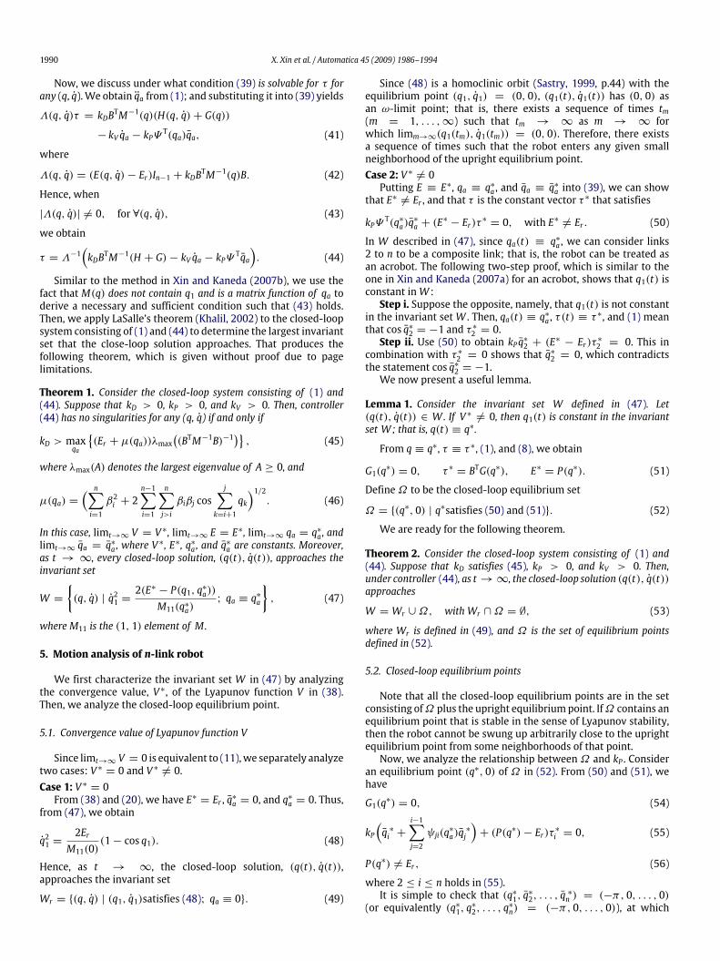
Fig. 5. Time responses of V and E − Er .

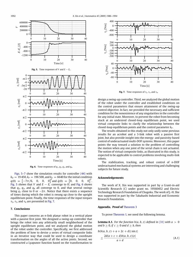
Fig. 6. Time responses of q1 , q2 , q3 , and q4 .

Figs. 5–7 show the simulation results for controller (44) withkD = 19 450, kP = 196 500, and kV = 6640 for the initial conditionq(0) =

[−7π/6, 0, 0, 0

]Tand q(0) = [0, 0, 0, 0

]T.Fig. 5 shows that V and E − Er converge to 0; and Fig. 6 showsthat q2, q3, and q4 all converge to 0, and that several swingsbring q1 close to 0 or −2π . Notice that there exists a sequenceof times during which the robot is swung up close to the uprightequilibrium point. Finally, the time responses of the input torquesτ2, τ3, and τ4 are presented in Fig. 7.

7. Conclusions

This paper concerns an n-link planar robot in a vertical planewith a passive first joint. We designed a swing-up controller thatbrings the robot into any arbitrarily small neighborhood of theupright equilibrium point, and we analyzed the global motionof the robot under the controller. Specifically, we first addressedthe problem of how to devise a series of virtual composite linksin an iterative way that could be used to design a coordinatetransformation on the angles of all the active joints. Second, weconstructed a Lyapunov function based on the transformation to

Fig. 7. Time responses of τ2 , τ3 , and τ4 .

design a swing-up controller. Third, we analyzed the globalmotionof the robot under the controller and established conditions onthe control parameters that ensure attainment of the swing-upcontrol objective. In fact, we provided the necessary and sufficientcondition for the nonexistence of any singularities in the controllerfor any initial state. Moreover, to prevent the robot from becomingstuck at an undesired closed-loop equilibrium point, we usedvirtual composite links to clarify the relationship between theclosed-loop equilibrium points and the control parameter kP .The results obtained in this study not only unify some previous

results for an acrobot and a 3-link robot with a passive firstjoint, but also provide insight into the energy- and passivity-basedcontrol of underactuatedmulti-DOF systems. Moreover, this paperpoints the way toward a solution to the problem of controllingthe motion when any one joint of the serial chain is not actuated.The notion of virtual composite links, as illustrated in this study, isexpected to be applicable to control problems involving multi-linkrobots.The stabilization, tracking, and robust control of n-DOF

underactuatedmechanical systems are interesting and challengingsubjects for future study.

Acknowledgements

The work of X. Xin was supported in part by a Grant-in-aidScientific Research (C) under grant no. 19560452 and ElectricTechnology Research Foundation of Chugoku. Thework of J.-H. Shewas supported in part by the Takahashi Industrial and EconomicResearch Foundation.

Appendix. Proof of Theorem 3

To prove Theorem 1, we need the following lemma.

Lemma A.1. For the function h(a, b, z) defined in (31) with a > 0and b ≥ 0, if c ≥ 0 and d ≥ b, then

b(h(a, b, z)+ a+ 2c + d)| sin z|

≤2d(a+ c + d)h(a, b, z)|z|

a+ d. (A.1)

X. Xin et al. / Automatica 45 (2009) 1986–1994 1993

Regarding statement 1), we carry out the proof by induction intwo steps:Step 1: For i = 2, we show that if

kP > km2 = 2β1n∑j=2

βj, (A.2)

then from (54) and (55), we obtainq∗1 = 0, or q∗1 = −π,q∗2 = 0, τ ∗2 = 0.

(A.3)

Step 2: Suppose that we have proved the following statement: Fori = k (k ≥ 2), if kP > max2≤j≤k kmj, where kmj is defined in (58),then onlyq∗1 = 0, or q∗1 = −π,q∗j = 0, τ ∗j = 0, for 2 ≤ j ≤ k (A.4)

satisfies (54) and (55) with i = k. For i = k + 1, we show that, ifkP > km(k+1) also holds, then the only solution to (55) for i = k+ 1is q∗k+1 = 0 and τ

∗

k+1 = 0.This proves that, when (57) holds, only (q∗1, q

∗

2, . . . , q∗n ) =

(0, 0, . . . , 0) and (q∗1, q∗

2, . . . , q∗n ) = (−π, 0, . . . , 0) satisfy (54)

and (55). Since the former contradicts (56), the latter is the onlysolution to (54)–(56).Regarding Step 1, first, we use (61) to rewrite (54) as

β1 sin q∗1 + β2∗sin(q∗1 + q

∗

2) = 0. (A.5)

τ ∗2 in (62) and P(q∗) in (60) yield

kpq ∗2 − β∗

2 (P(q∗)− Er) sin(q∗1 + q

∗

2 ) = 0, (A.6)

where

P(q∗) = β1 cos q∗1 + β2∗cos(q∗1 + q

∗

2). (A.7)

Adding P2(q∗) to the square of (54) gives

P2(q∗) = h2(β1, β∗2 , q∗

2). (A.8)

From (A.5) and (A.7), we obtain

P(q∗) sin(q∗1 + q∗

2) = β1 sin q∗

2. (A.9)

Therefore, if P(q∗) 6= 0, then we use (A.8) and (A.9) to eliminate q∗1from (55) to obtain

kPβ1q∗2 =

β ∗2

(h(β1, β ∗2 , q

∗

2)− sgn(P(q∗))Er

)sin q∗2

h(β1, β ∗2 , q∗

2), (A.10)

where sgn(P(q∗)) denotes the sign of P(q∗).Now we show that P(q∗) 6= 0 under (A.2). First, suppose the

opposite, namely, that P(q∗) = 0. Then, from (A.8), we havecos q∗2 = −1 and β1 = β

∗

2 . This reduces (A.6) to

kP q∗2 − β1Er sin q∗

1 = 0. (A.11)

From cos q∗2 = −1, we obtain q∗

2 = ±π,±3π, . . .. From β1 = β∗

2 ,it follows that themechanical parameters of the robot must satisfyβ1 = β ∗2 ≤

∑nj=2 βj and Er = β1 +

∑nj=2 βj ≤ 2

∑nj=2 βj. Thus,

under (A.2), we obtain

kPβ1Er|q∗2| >

2n∑j=2βj

Er|q∗2| ≥ |q

∗

2| ≥ π > | sin q∗

1|,

which contradicts (A.11). Thus, P(q∗) 6= 0 under (A.2).Next, clearly q∗2 = 0 is a solution to (A.10) for any β

∗

2 . To applyLemma A.1, we define z = q∗2 , a = β1, b = β ∗2 , c = 0, and

d =∑nj=2 βj. That gives us Er = a + d and d ≥ b. Thus, when

q∗2 6= 0, we can rewrite (A.10) as

kPβ1=

b(h(a, b, z)− sgn(P(q∗))(a+ d)

)sin z

h(a, b, z)z. (A.12)

It follows directly from Lemma A.1 that

b(h(a, b, z)+ a+ d

)| sin z|

h(a, b, z)|z|≤2d(a+ d)a+ d

=km2β1. (A.13)

Thus, only q∗2 = 0 satisfies (A.10) under (A.2).When q∗2 = 0, (A.5) yields sin q∗1 = 0. This gives us τ ∗2 =

G2(q∗) = −β ∗2 sin(q∗

1 + q∗

2 ) = 0, thereby showing that (A.3) istrue. Moreover, from (A.7), we haveP(q∗) = β1 + β ∗2 > 0, if q∗1 = 0,P(q∗) = −β1 − β ∗2 < 0, if q∗1 = −π.

(A.14)

Regarding Step 2, since q ∗2 = · · · = q∗

k = 0 owing to (A.4), wecan simplify (55) for i = k+ 1 to

kP q ∗k+1 + (P(q∗)− Er)τ ∗k+1 = 0. (A.15)

Using (A.4), (A.14), and P(q∗) in (60), we obtain

|P(q∗)| = β1 + · · · + βk−1 + β∗k . (A.16)Regarding τ ∗k+1, from τ

∗

k = Gk(q∗) andGk(q) in (7), and from τ ∗k = 0

owing to (A.4), we have τ ∗k+1 = βk sin(q∗

1+· · ·+q∗

k). From (23) and(A.4), for k ≥ 2 we have q∗k = q

∗

k − θ∗

k+1 = −θ∗

k+1 and for k ≥ 3we haveθ∗3 = · · · = θ

∗

k = 0, q∗2 = · · · = q∗

k−1 = 0. (A.17)Thus, τ ∗k+1 = βk sin(q

∗

1 − θ∗

k+1). Using (A.14) yields

τ ∗k+1 = −sgn(P(q∗))βk sin θ∗k+1. (A.18)

We can use the formula for sin θk+1 in (26) and β ∗k =

h(βk, β ∗k+1, q∗

k+1) to reduce (A.15) to

kPβkq ∗k+1 =

β ∗k+1(|P(q∗)| − sgn(P(q∗))Er) sin q ∗k+1h(βk, β ∗k+1, q

∗

k+1). (A.19)

Clearly, q∗k+1 = 0 is a solution to (A.19). To use Lemma A.1,we define z = q∗k+1, a = βk, b = β ∗k+1, c =

∑k−1j=1 βj, and

d =∑nj=k+1 βj. That gives us d ≥ b and Er = a + c + d. When

q ∗k+1 6= 0, we rewrite (A.19) as

kPβk=

b(h(a, b, z)− sgn(P(q∗))(a+ 2c + d)

)sin z

h(a, b, z)z. (A.20)

It follows directly from Lemma A.1 that

b(h(a, b, z)+ a+ 2c + d

)| sin z|

h(a, b, z)|z|≤2dEra+ d

. (A.21)

Thus, if kp > km(k+1), then (A.20) has no solution; that is, (A.19)has the unique solution q∗k+1 = 0. This yields θ∗k+1 = 0, thuscompleting Step 2.Regarding statement 2), letting (−π + δ, 0, . . . , 0) be a point in aneighborhood of the downward equilibrium point yields V (−π +δ, 0, . . . , 0) = (1 + cos δ)2E2r /2 < V (−π, 0, . . . , 0) for δ 6∈0,±2π, . . .. Since V is non-increasing under controller (44),according to Theorem 2, no matter how small |δ| > 0 is, ann-link robot starting from (−π + δ, 0, . . . , 0) will not approach(−π, 0, . . . , 0), but will approachWr instead. This shows that thedownward equilibrium point is unstable.Regarding statement 3), it is a direct consequence of statement 1)and Theorem 2.

1994 X. Xin et al. / Automatica 45 (2009) 1986–1994

References

Acosta, J. A., Ortega, R., Astolfi, A., & Mahindrakar, A. D. (2005). Interconnectionand damping assignment passivity-based control of mechanical systems withunderactuation degree one. IEEE Transactions on Automatic Control, 50(12),1936–1955.

Arai, H., Tanie, K., & Shiroma, N. (1998). Nonholonomic control of a three-DOF planarunderactuated manipulator. IEEE Transactions on Robotics and Automation,14(5), 681–695.

Arikawa, K., & Mita, T. (2002). Design of multi-DOF jumping robot. In Proceedings ofIEEE international conference on robotics and automation (pp. 3992–3997).

Åström, K. J., & Furuta, K. (2000). Swinging up a pendulum by energy control.Automatica, 36(2), 287–295.

De Luca, A., & Oriolo, G. (2002). Trajectory planning and control for planar robotswith passive last joint. International Journal of Robotics Research, 21(5–6),575–590.

Fantoni, I., Lozano, R., & Spong, M.W. (2000). Energy based control of the Pendubot.IEEE Transactions on Automatic Control, 45(4), 725–729.

Ge, S. S., Wang, Z. P., & Lee, T. H. (2003). Adaptive stabilization of uncertainnonholonomic systems by state and output feedback. Automatica, 39(8),1451–1460.

Gonzalez-Hernandez, H. G., Alvarez, J., & Alvarez-Gallegos, J. (2004). Experimentalanalysis and control of a chaotic pendubot. International Journal of RoboticsResearch, 23(9), 891–902.

Grizzle, J.W.,Moog, C. H., & Chevallereau, C. (2005). Nonlinear control ofmechanicalsystems with an unactuated cyclic variable. IEEE Transactions on AutomaticControl, 50(5), 559–575.

Hauser, J., & Murray, R.M. (1990). Nonlinear controllers for non-integrable systems,the Acrobot example. In Proceedings of American control conference (pp.669–670).

Hyon, S. H., Yokoyama, N., & Emura, T. (2006). Back handspring of a multi-linkgymnastic robot—Referencemodel approach. Advanced Robotics, 20(1), 93–113.

Jiang, Z. P. (2002). Global tracking control of underactuated ships by Lyapunov’sdirect method. Automatica, 38(2), 301–309.

Khalil, H. K. (2002). Nonlinear systems (3rd ed.). New Jersey: Prentice-Hall.Kolesnichenko, O., & Shiriaev, A. S. (2002). Partial stabilization of underactuatedEuler–Lagrange systems via a class of feedback transformations. Systems &Control Letters, 45(2), 121–132.

Lin,W., Pongvuthithum, R., & Qian, C. J. (2002). Control of high-order nonholonomicsystems in power chained form using discontinuous feedback. IEEE Transactionson Automatic Control, 47(1), 108–115.

Ortega, R., & Spong,M.W. (1989). Adaptivemotion control of rigid robots: A tutorial.Automatica, 25(6), 877–888.

Ortega, R., Spong,M.W., Gomez-Estern, F., & Blankenstein, G. (2002). Stabilization ofa class of underactuated mechanical systems via interconnection and dampingassignment. IEEE Transactions on Automatic Control, 47(8), 1218–1233.

Reyhanoglu, M., van der Schaft, A., McClamroch, N. H., & Kolmanovsky, I. (1999).Dynamics and control of a class of underactuated mechanical systems. IEEETransactions on Automatic Control, 44(9), 1663–1671.

Sastry, S. (1999). Nonlinear systems: Analysis, stability, and control. New York:Springer.

Shkolnik, A., & Tedrake, R. (2008). High-dimensional underactuated motionplanning via task space control. Proceedings of IEEE/RSJ international conferenceon intelligent robots and systems (pp. 3762–3768).

Spong, M. W. (1995). The swing up control problem for the Acrobot. IEEE ControlSystems Magazine, 15(1), 49–55.

Spong, M. W., & Block, D. J. (1995). The Pendubot, a mechatronic system for controlresearch and education. In Proceedings of the 34th IEEE conference on decision andcontrol (pp. 555–556).

Spong, M. W. (1996). Energy based control of a class of underactuated mechanicalsystems. In Proceedings of 1996 IFAC world congress (pp. 431–435).

Spong, M. W. (1998). Lecture notes in control and Information Sciences: Vol. 230.Underactuated mechanical system. Berlin: Springer.

Wiklund, M., Kristenson, A., & Åström, K. J. (1993). A new strategy for swingingup a pendulum by energy control. In Preprints of IFAC 12th world congress (pp.151–154).

Yeadon, M. R., & Hiley, M. J. (2000). The mechanics of the backward giant circle onthe high bar. Human Movement Science, 19(2), 153–173.

Xin, X., & Kaneda, M. (2005). Analysis of the energy based control for swinging uptwo pendulums. IEEE Transactions on Automatic Control, 50(5), 679–684.

Xin, X., & Kaneda, M. (2007a). Analysis of the energy based swing-up controlof the Acrobot. International Journal of Robust and Nonlinear Control, 17(16),1503–1524.

Xin, X., & Kaneda, M. (2007b). Swing-up control for a 3-DOF gymnastic robotwith passive first joint: Design and analysis. IEEE Transactions on Robotics andAutomation, 23(6), 1277–1284.

Xin Xin received the B.S. degree in 1987 from theUniversity of Science and Technology of China, Hefei,China, and Ph.D. in 1993 from the Southeast University,Nanjing, China. From 1991 to 1993, he did his Ph.D. studiesin Osaka University as a co-advised student of China andJapan with the Japanese Government Scholarship. He alsoreceived the Doctor degree in engineering in 2000 fromTokyo Institute of Technology.From 1993 to 1995, he was a postdoctoral researcher

and then became an associate professor in SoutheastUniversity. From 1996 to 1997, he was with the New

Energy and Industrial Technology Development, Japan as an advanced industrialtechnology researcher. From 1997 to 2000, he was a research associate at theDepartment of Control and Systems Engineering, Tokyo Institute of Technology.From 2000, he has been with Okayama Prefectural University as an associateprofessor, where he has been a professor since 2008. He has also been a visitingprofessor of Southeast University since 2004. He has over 100 publications injournals, international conferences and book chapters. He received the divisionpaper award of SICE 3rd Annual Conference on Control Systems in 2004. His currentresearch interests include robotics, dynamics and control of nonlinear and complexsystems.

Jin-Hua She received a B.S. in engineering from CentralSouth University, Changsha, Hunan, China, in 1983, andan M.S. in 1990 and a Ph.D. in 1993 in engineeringfrom the Tokyo Institute of Technology, Tokyo, Japan. In1993, he joined the Department of Mechatronics, Schoolof Engineering, Tokyo University of Technology; and inApril, 2008, he transferred to the University’s School ofComputer Science, where he is currently an associateprofessor. He received the control engineering practicepaper prize of the International Federation of AutomaticControl (IFAC) in 1999 (jointlywithM.WuandM.Nakano).

His research interests include the application of control theory, repetitive control,process control, Internet-based engineering education, and robotics.

Taiga Yamasaki received a Ph.D. degree in engineering,from Osaka University in 2003. From 2000 to 2003,he was a research fellow of the Japan Society forthe Promotion of Science. He is currently an assistantprofessor in Department of Systems Engineering at theOkayama Prefectural University. His current interests arein computational motor control in humans and robots,especially gymnastic movements on the high bar, bipedlocomotion, and other nonlinear control mechanisms ofneuro-musculo-skeletal systems.

Yannian Liu received the B.S. degree in electrical engi-neering from Sichuan University, Chengdu, China in 1988,and theM.S. and Ph.D. from Southeast University, Nanjing,China in 1991 and 1994, respectively. From 1994–1995she was a postdoctoral researcher in Nanjing University ofAeronautics and Astronautics. From 1996 she was an as-sociate professor in the Control Department of SoutheastUniversity. From 1997 to 1999, she was a visiting scholarin the Department of Control and Systems Engineeringof Tokyo Institute of Technology. She is now working inthe Solution Division of MoMo Alliance Co., Ltd. Okayama,

Japan. Her current research interests include robotics and control technologies forLED.