Sustainable Forest Management for Small Farmers in Acre...
207
1 Sustainable Forest Management for Small Farmers in Acre State in the Brazilian Amazon by Marcus Vinicio Neves d’Oliveira Supervisors: M.D. Swaine And David F.R.P. Burslem A thesis submitted to the University of Aberdeen for the Degree of Doctor of Philosophy Department of Plant & Soil Science February 2000 University of Aberdeen
Transcript of Sustainable Forest Management for Small Farmers in Acre...

1
Sustainable Forest Management for Small Farmers in Acre State in the Brazilian
Amazon
by
Marcus Vinicio Neves d’Oliveira
Supervisors:
M.D. Swaine
And
David F.R.P. Burslem
A thesis submitted to the University of Aberdeen for the Degree of Doctor of Philosophy
Department of Plant & Soil Science February 2000 University of Aberdeen

2
Declaration
I hereby declare that the work presented in this thesis has been performed by myself
in the department of Plant and Soil Science, University of Aberdeen, and that it has
not been presented in any previous application for a degree. All verbatum extracts
have been distinguished by quotation marks and all sources of information
specifically acknowledged by reference to the authors.
Marcus Vinicio Neves d’Oliveira

3
Acknowledgements
I would like to express my gratitude to the following:
Dr. M.D Swaine and Dr. D.F.R.P. Burslem, my supervisors, for their help, friendship
and especially for their patience correcting this thesis.
EMBRAPA, Dr. Judson Ferreira Valentim and the other directors of the CPAF-ACRE,
for the support in all moments, especially during the field work.
CNPq for the scholarship and University expenses.
Paulo Carvalho, Airton Nascimento, Airton F. Silva, Rosivaldo Saraiva, Francisco
Abomorad “mateiros” and technician, members of the field work team from CPAF-
ACRE and the “mateiros” Ivo Flores and Raimundo Saraiva from FUNTAC, for their
assistance on the species identification, patience, suggestions and tireless work.
The other members of the PC Peixoto Forest Management Project in Brazil Evaldo
Muñoz Braz and Henrique J.B. de Araujo.
My friends in the department especially Tim Baker (who first introduced me to fish
and chips), David Genney and the “brasileiros” Fabio Chinaglia and Rose Dams for
their friendship and suggestions for this work.
Dr. Jose Natalino Macedo da Silva and Dr. Niro Higuchi, for the support and
incentive they gave to me to start my PhD studies and Dr. Richard W. Bruce, who
introduce me to the Abufari people and Abufari forest, where was born the idea to
develop this forest management system.
My parents who have been a great encouragement throughout my studies, my
brother Julio and my nephew Michel.
Lastly, but never least, to my wife Mauricilia “Monstra” (also using this space to
apologise for the fact that I did not write the Chapter she asked me to write, only to
acknowledge her, and recognise that she surely deserved it), for the encouragement,
support, love etc and Maria João just for being a very nice girl.

4
Summary
This thesis has the aim of presenting a forest management system to be applied on small farms, especially in the settlement projects of the Brazilian Amazon, and to examine its sustainability by investigating the responses of the forest in terms of the changes in natural regeneration in felling gaps and the dynamics of the residual trees. Using the program CAFOGROM, an additional aim was to simulate the forest responses to different cycle lengths, harvesting intensities and silvicultural treatments to determine the theoretical optimum combination of these parameters. The proposed forest management system was designed to generate a new source of family income and to maintain the structure and biodiversity of the legal forest reserves. The system is new in three main characteristics: the use of short cycles in the management of tropical forest, the low harvesting intensity and environmental impact and the direct involvement of the local population in all forest management activities. It is based on a minimum felling cycle of ten years and an annual harvest of 5-10 m3 ha-1 of timber. The gaps produced by logging in PC Peixoto can be classified as small or less often medium sized (canopy openness from 10% to 25%). Differences in gap size and canopy openness produced significant differences in the growth rates, species richness and species diversity of seedlings established in the gaps. Mortality rates of seedlings in the artificial gaps increased and recruitment rates decreased with increasing gap size. The density and recruitment of seedlings of commercial species was not different between gap sizes, but gap creation increased the growth rate of the seedlings of these species. Small and medium gaps (less than 25 % canopy openness) improved regeneration from the forest management point of view, with fewer pioneer plants, higher diversity and lower mortality, although they resulted in lower seedling growth rates. The mean periodic annual diameter increment of trees in the permanent sample plots (0.27 cm yr-1) and mean annual mortality rates (2.1 % yr-1) were similar to those found by other research in the tropics. Differences in species growth between crown exposure and species groups were statistically significant. The influence of management was positive in terms of diameter increment increase in both mechanised and non-mechanised forest management systems. The volume increment of commercial species for both kinds of forest management is compatible with the logging intensity and cycle length proposed, and the density and recruitment of commercial species were not affected by logging. Ten year cycles were the most appropriate compromise among the studied cycle length for sustainable forest management under the conditions examined in this study. A regular harvesting of 8 to 10 m3 ha-1 cycle-1 can be expected with the combination of a harvesting intensity of around 1.0 m2 ha-1 cycle-1 and silvicultural treatments removing around 1.5 m2 ha-1 cycle-1. However, the results of the simulations must be interpreted as indications of the behaviour of the forest in response to different interventions rather than as quantitative predictions. The project will continue as a part of the EMBRAPA research programme, and receiving additional support from the ASB (alternative to slash and burn) project. The continuation of the project will allow the continuation of research on forest dynamics and plant succession in the felling and artificial gaps.

5
CHAPTER 1
Sustainable Forest Management: an option for land use in
Amazon
1.1 Introduction
The world’s forest resources are being depleted or degraded for a variety of reasons.
Commercial logging without a silviculture-based management plan, slash and burn
agriculture, and cattle pasture establishment or other non-forest enterprises are
among the main reasons for deforestation in the tropics (Whitmore, 1992). The major
cause of uncontrolled use and misuse of tropical forests is the dependency of
millions of rural people on forest resources, and the soil that they cover, for basic
needs of food, energy and shelter (Hendrison, 1990).
It has been estimated that tropical rain forests have been converted at a rate
of 15.4 million hectares a year over the period 1981 – 1990 (FAO, 1993) and 13.7
million hectares a year over the period 1990 – 1995 (FAO, 1997, 1999). The profits
that come from alternative uses of the land, such as shifting cultivation, are greater
than the use of these original ecosystems for forest management practices (Higuchi,
1994). In addition, even when managed, the increased access provided by forest
harvesting (e.g. by skid trails) and demographic pressures after the first harvesting,
means that forests are more likely to be converted than conserved.
At the end of 1990, 76 % of the tropical rain forest zone still remained intact,
but the annual loss of biomass was estimated at slightly over 2,500 million tonnes, of
which more than 50 % percent was contributed by Latin America, nearly 30 % by
tropical Asia and about 20 % by tropical Africa (FAO, 1993). In both Brazil and
tropical Asia, change from continuous forests occurs at a rate much higher than in
tropical Africa, owing to the higher population density in Asia and planned
resettlements/resource exploitation programmes (in Brazil and Asia) (FAO, 1993). In
this way, tropical timber resources have been decreasing sharply in the recent past,
especially in Southeast Asia (FAO, 1993), where traditional timber exporting
countries are reducing or even banning (e.g. Thailand) timber harvesting activities
(Johnson, 1997).
The decrease in the amount of timber production is in conflict with the
growing demand from the furniture manufacturing and secondary processing
industries, that has generated a substantial increase in timber imports in many

6
countries. In general, both exportation and importation of tropical timber have
declined in recent years, and only in South America is production still increasing
(Johnson, 1997).
It seems likely that in the near future the focus of tropical timber production
will change to South America. An important issue in this context is that while for the
most important commercial timber species, prices are dropping in Asia (e.g. for
Shorea spp, from US$800 per m3 in 1993 to US$600 in 1995) and Africa (e.g. for
Entandrophragma utile, from US$750 per m3 in 1993 to US$600 in 1994), the prices
for the most important South American species (Swietenia macrophylla) remain
constant, and will probably increase because of the ban on new concessions for
Swietenia macrophylla and Virola spp in Brazil (Johnson, 1997). On the other hand
there is a growing international pressure for the preservation of tropical forests.
Proposals such as Target 2000 (ITTO, 1991) attempt to ensure that only wood from
sustainably managed tropical forests is allowed to enter international markets. The
idea that the forest must be preserved as a sanctuary has been replaced by a more
realistic one where by it is argued that the only way to promote conservation of an
ecosystem is by giving it a economic function (Barros and Uhl, 1995; FAO, 1998). All
these factors would favour the development of forest management activities in South
America.
However, the scientific understanding of tropical forest ecosystems is still far
from complete. There is an urgent need to develop ecologically sound sustainable
management techniques. Ecologically based management for sustainable harvesting
requires, at a minimum, three types of measurements: (i) monitoring the effects of the
logging practices on the composition and structure of the residual stand; (ii)
estimates of the parameters of growth and survival that determine recruitment into
harvestable sizes during stand development after logging; (iii) the density and
composition of regeneration (Cannon et al. 1994).
Forest management is needed at two scales: management for large areas
without heavy human population pressure and management for small areas in
inhabited areas (Braz and Oliveira, 1994). In the first case, the traditional forest
management systems, allied to governmental policies and legislation, are sufficient to
achieve success. However, in the second case, specific techniques, policies, criteria
and legislation must be created in most countries.
In this thesis I will present a forest management system for application on
small farms, in the settlement projects of the Brazilian Amazon, and examine its
sustainability by monitoring regeneration in felling gaps and the dynamics of the
residual trees. Using the program CAFOGROM (Alder, 1995a, 1995b; Alder and

7
Silva, 1999), an additional aim is to simulate the response of the forest to different
felling cycle lengths, harvesting intensities and silvicultural treatments in order to
determine the theoretical optimum combination of these variables.
The objectives of this chapter are to provide an overview of the history and
perspectives of forest management in the tropics, to review the most widely used
silvicultural systems and to discuss their characteristics and constraints in the West
Amazon tropical forest context.
1.2 Important silvicultural systems used in tropical forests
Many silvicultural systems have been developed and tested for tropical rain forest.
These are briefly reviewed below in order to present possible option for small farmers
in Amazon. Reviews of tropical silvicultural systems have been published (e.g.
Jonkers, 1987; Silva, 1989, 1997, Higuchi, 1994; Philip and Dawkins, 1998). In
summary, silvicultural systems were derived from the Selection System, in which part
of the stand is harvested every 20-40 years or the Uniform System, in which the
entire population of the marketable trees are removed in a single harvest. Many
variations exist between these extremes. The most important in tropical forest
silviculture are the various types of Shelterwood Systems, in which the leap from one
rotation to another is neither as abrupt as in the Uniform System nor as prolonged as
in the Selection System (Philip and Dawkins, 1998). The main characteristics of
some of these systems are presented in Table 1.2.
There are also the semi-natural silvicultural methods, that create relatively
even-aged stands similar to tree plantations after the total or partial removal of the
original forest in one or more operations. These methods include the Taungya
system (felling of demarcated areas of forest and planting of food crops and
desirable species, originally applied in Myanmar) the Limba-Okume system (after
clear-cutting the forest, Terminalia superba and Aucoumea klaineana are planted;
introduced in West Africa), the Martineau system (systematic replacement of the
natural heterogeneous forest by an even-aged plantation of valuable species, applied
in extensive areas in Côte d’ Ivoire) and the Recrû system (replacement of the forest
in two steps, first by cutting shrubs and small trees up to 15-20 cm and second by
poison-girdling of all or part of the remaining standing trees, used in Gabon). Other
methods that involve planting, are “line planting” (planting of seedlings in opened
lines in the forest) and the Placeaux method (planting of tree seedlings in 4 x 4 m
plots spaced at 10 m intervals). All these techniques have been reviewed and
described by Silva (1989, 1997).

8
Table 1.2: Main characteristics of the most well known silvicultural systems applied in tropical forests. Silvicultural system Main characteristics References The selective system Policyclic system; part of the stand is harvested ever 20 to 40
years after liana cutting to reduce damage during forest exploitation
Jonkers, 1982; 1987; Silva, 1989; Higuchi, 1994; Dawkins and Philip, 1998
The Indonesian selective system
Policyclic system; minimum felling diameter 50 cm dbh; cycle length 35 years; harvesting intensity around 70 m3 ha-1
Sudino and Daryadi, 1978; Whitmore, 1984
Selective logging system (Philippines)
Removal of all trees above 75 cm dbh; 70 % of the trees in the classes from 15-65 cm dbh and of the 70 cm dbh class are left as residuals; cycle length 20 to 40 years.
Virtucio and Torres, 1978; Reyes, 1978b; Silva, 1989
The Malayan Uniform System (MUS)
Monocyclic system involving the harvesting of all marketable trees; understorey cleaning two years after logging; thinning 10 years after logging repeated at intervals of 15 to 20 years; cycle length from 60 to 80 years
Wyatt-smith, 1963; Jonkers, 1987; Higuchi, 1994;
MUS modified for Sabah Bicyclic system where some commercial trees are retained to provide an intermediate harvesting 40 years after the first harvesting; felling diameter limit fixed at 60 cm dbh
Ting, 1978; Munang, 1978; Schmidt, 1987, 1991; Thang, 1987; Mok, 1992
The Tropical Shelterwood System
Shelterwood systems involve successive regeneration fellings; old trees are removed by two or more successive fellings resulting in a crop that is more or less uneven
Lowe, 1978; Matthew, 1989; Higuchi, 1994
Andaman Canopy Lifting System
Harvesting of commercial trees above 63 cm; crown thinnings conducted at 6, 15, 30 and 50 years
Lowe, 1978; Thangman, 1982; Silva, 1989
The CELOS system Policyclic system designed to produce around 20 m3 ha-1 in cycles of 20 years where the increment of the residual trees of commercial species is stimulated by several refining treatments during the felling cycle
De Graaf, 1986; De Graaf and Poels, 1990; De Graaf and Rompaey, 1990; Hendrison, 1990; Van Der Hout, 1999

9
A consensus now exists regarding the relative suitability of these systems for
tropical forest management. Uniform systems have been gradually abandoned as it
has become clear that they are unsuitable for sustained yield tropical forest
management (Cheah, 1978; Higuchi, 1994; Dawkins and Philip, 1998). This
unsuitability derives from the long length of the felling cycles and large areas of forest
demanded (Thang, 1987). In addition, the heavy impact on forest structure means
that uniform systems are only feasible when there is dense regeneration of desirable
species and it is possible to implement silvicultural treatments (Lee, 1982, Jonkers,
1987). However, exceptions are still being applied such as the Strip Harvesting
System in Palcazu Peru (Ocaña-Vidal, 1992).
Silvicultural systems such as the Tropical Shelterwood System and Selection
System, which were developed, refined and used in Asia, are appropriate for most
tropical forest regions on technical grounds. When appropriate management
techniques are applied, growth and yield models suggest that there is no decline in
forest productivity over a number of cycles (e.g. Vanclay, 1990). However, forest
management has often failed as a result of factors such as land use pressure (e.g.
Hon and Chin, 1978), illegal timber harvesting (Silva, 1989) and undervaluation of the
forest resource. Two of the most important reasons for the failure of forest
management are the lack of participation of local communities in the forest
management activities and the long felling cycles. In addition, there are political,
economic and social factors that must be considered alongside of the silvicultural
factors (Whitmore, 1992).
The silvicultural systems presented above have some common
characteristics such as long cutting cycles of 20 years or more, a requirement for
implementation over large areas and a high demand for technology. Mechanisation
requires heavy investment and prevents the local populations becoming involved. In
addition, these systems involve silvicultural treatments before and after harvesting,
and long-term investments which, allied with the unstable economies of many tropical
countries, make forest management economically unattractive and difficult to
implement, even on a large scale.
1.3 Community management systems
The felling and extraction of trees and other products in tropical forests is a traditional
practice of the local people in the Amazon (Oliveira, 1989, 1992) and other tropical
countries. For example in Indonesia, trees with diameters above 60 cm dbh are felled
in strips of about 2 km in width along rivers, leaving a dense residual stand. However,

10
there has been a trend towards large scale logging operations in many tropical
countries (Sudiono and Daryadi, 1978).
Although few of the techniques were designed specifically to be applied in
collaboration with local communities, some attempts are being made in several
places to make forest management possible at this level for sustainable production of
timber and non-timber products (Perl et al. 1991; Batoum and Nkie, 1998). These
activities usually develop in secondary forests (e.g. Castañeda et al. 1995) because
the use of animal traction only allows the extraction of relatively small diameter logs.
Some attempts have also been made to work in primary forests. In this case
the effective participation of the community is often limited and all activities are
performed by third parties (e.g. lumber merchants). In some cases, the forest is
bought by private enterprises that employ some of the community members (e.g.
Tecnoforest del Norte in the Portico Project, Perl et al. 1991). In addition, competition
from large enterprises usually prevents small farmers from working in primary forests
because of the need to use heavy machinery for extraction of logs.
The involvement of the local population in forest management is an important
factor in meeting the original objectives of forest management (Dickinson et al.
1996). Some systems designed for forest communities have been applied in Latin
America with some success. These include the Boscosa project in Costa Rica (Perl
et al. 1991; Howard, 1993), and the strip clear-cutting system developed in Costa
Rica (Ocaña-Vidal, 1992), both of which had the effective involvement of the local
population. The BOSCOSA project is carried out in the Osa peninsula in Costa Rica.
It is an integrated management project that includes agroforestry, agriculture and
forest management (Kierman et al. 1992). The silvicultural prescriptions consist of
two phases, termed conversion and maintenance. The conversion phase consists of
in two or three conversion cuttings at 10 or 15 year intervals involving the removal of
trees larger than 60 cm diameter. During the maintenance phase, a fixed percentage
of the number of trees in diameter classes between 30 and 60 cm dbh is taken at
each cutting (Howard, 1993). The cycle length is 15 to 25 years with an estimated
production of around 20 m3 ha-1 cycle-1 (Perl et al. 1991). Strip clear-cutting was
developed by the Tropical Science Centre in Costa Rica. The forest is harvested in
long, narrow clear-cuttings designed to mimic natural disturbance caused by the fall
of a single large tree. Natural regeneration is monitored over a period of 40 to 50
years (Ocaña-Vidal, 1992). The strips vary in width from 30 to 50 m and the
harvesting includes all trees with diameter greater than 5 cm using animal power for
log extraction (Ocaña-Vidal, 1992).

11
Small properties typically only produce small quantities, which is enough to
meet the owner’s needs and provide for the demands of local markets. Both the
production and the quality of the products are usually low, but those factors can be
improved in small-scale enterprises through the organisation of the work into co-
operatives that allow technology to be acquired and products to be accumulated.
1.4 Land use and forest management in the Amazon
The great majority of deforestation in the Brazilian Amazon is followed by conversion
of land to castle pasture, either immediately or after 1-2 years of use under annual
crops (ranchers are responsible for about 70 % of this practice and small immigrant
farmers 30 %) (Fearnside, 1995). In the Brazilian Amazon, the rate of deforestation
varies very much from place to place, and usually follows logging of the forest.
The Amazon experienced a high deforestation rate from the end of the 1970s
to the end of the 1980s. A drastic reduction in the rate of deforestation was observed
between 1988 and 1992, because of economic instability and the ending of financial
credits for the clearance of forest for pastures in Amazon in 1990. From 1992 to 1995
the deforestation rate increased again following introduction of the “Plano Real” for
the economy which stabilised the currency and favoured investments in the region.
However, from 1995 to 1997 a decline in the deforestation rate was promoted by an
economic crisis (INPE, 1998). In general, the deforestation rate has shown a
tendency to decrease over time. The fluctuations in deforestation rates have been
promoted more by the economic environment than by external pressures or the
implementation of land use policies for Amazon (Table 1.1).
Table 1.1 Mean rate of gross deforestation (km2 year-1) from 1978 to 1997 in the Brazilian
Amazon*.
Amazon States
77-881
88-89 89-90 90-91 91-92 92-942
94-95 95-96 96-97
Acre 620 540 550 380 400 482 1208 433 358 Amapá 60 130 250 410 36 - 9 - 18 Amazonas 1510 1180 520 980 799 370 2114 1023 589 Maranhão 2450 1420 1100 670 1135 372 1745 1061 409 Mato-Grosso
5140 5960 4020 2840 4674 6220 10391 6543 5271
Pará 6990 5750 4890 3780 3787 4284 7845 6135 4139 Rondônia 2340 1430 1670 1110 1110 2595 4730 2432 1986 Roraima 290 630 150 420 420 240 220 214 184 Tocantins 1650 730 580 440 440 333 797 320 273 Amazon 21130 17860 13810 11130 13786 14896 29059 18161 13227 * All data from INPE, 1998. 1. decade mean; 2. biennial mean

12
The east Amazon, especially along the Belém to Brasilia and Cuiabá to
Santarém roads, experienced heavy deforestation during the 1970s and 1980s,
usually from logging followed by conversion to shifting cultivation and pasture
formation (Uhl and Vieira, 1988; Homma et al. 1993). Rondônia State in west
Amazon followed the same pattern of deforestation and land use change along the
BR364 road as that described above. This State has the highest percentage of
deforested land in the Amazon, that is, about 14 % of the total forest area (FAO,
1993).
When deforestation in Acre State began, it followed the same pattern as in
Rondônia and east Pará (the Paragominas region). The BR364 road crosses Acre
State for more than 700 km, linking Rio Branco to Cruzeiro do Sul and other State
roads linking Rio Branco to cities such as Xapuri, Assis Brasil and Brasiléia on the
border with Bolivia. Deforestation in Acre State is about 9 % of the total forest area
(INPE, 1998) and is highly concentrated in the Acre river valley (FUNTAC, 1990).
Alternative land uses that preserve the forest, such as extractivism, are
difficult to implement in Amazon because the rubber produced from native forest
extraction is not competitive with imports from Southeast Asia in the absence of trade
barriers (Fearnside 1995). It will take some time before markets develop for the other
non-timber forest products that the Amazon forest has to offer (Barros and Uhl,
1995). Selective logging on a rotational basis is another activity that has a relatively
low environmental impact on the forest (Uhl & Bushbacher, 1988). However,
selective logging is also the first step in forest conversion, as it provides a subsidy for
the creation and maintenance of croplands and pastures. The harvesting of
marketable wood was used, and sometimes still is used, as an accessory activity to
finance pasture formation. These activities are the main reason for the poor
reputation of forestry in the Amazon, despite the fact that selective logging, in the
absence of following any silvicultural intervention, preserves the structure of the
forest rather than compromising the entire ecosystem by replacing forest with crops
and pastures.
In the Brazilian Amazon, forest management is monitored and controlled by
the Brazilian Institute for Environment and Natural Resources (IBAMA) through a
document called “Forest Management Plan”, which must be prepared in advance by
the farmers or companies and approved by the Institute. However, because of the
structural and manpower constraints on IBAMA and the large areas of forest in the
Brazilian Amazon, the execution of forest management does not usually follow any
silvicultural system. For example, in practice, the prescribed silvicultural treatments
are very often not applied (EMBRAPA, 1996). The first official attempt to establish

13
forest management in Brazil was in 1965 with the publication of the new Brazilian
Forest Code (Law 4771), which banned the use of the native forests unless a
management plan was in place. However, Article 15, which was supposed to specify
the silvicultural techniques required for sustainable forest management, was only
approved in 1992 (Silva, 1992). During the intermediate period forest management
was poorly regulated through governmental decrees which were technically brief and
contributed little to the implementation of the appropriate use of the natural forests.
Several forest management plans have been developed for the Amazon since then,
especially in Pará State, east Amazon, and Mato-Grosso State in the southern
Amazon (Leite, 1995). In practice, these plans have been rarely implemented and
frequently they acted only as a formal authorisation for forest exploitation without the
use of any silvicultural technique because exploitation was not controlled or
adequately policed.
In Brazil the concept of sustainable yield management was introduced by
FAO experts, who performed the first forest inventories in the 1950s. Forest
management research started in the late 50s in the Curuá-Una forest on a project
where Brazilian researchers from SUDAM worked with FAO researchers (SUDAM,
1978). This project was later extended to the FLONA (National Forest) Tapajós in
Pará State (Silva, 1989). Pilot projects on forest management research are currently
being carried out in Amazon. As well as the work been conducted by CPATU in
FLONA Tapajós, the two other initiatives continuing in Pará State are managed by
IMAZON and TFF (Tropical Forest Foundation). In Amazonas State about 80,000 ha
of terra-firme forest is being managed by an international project (Precious Wood
project, personal observation) near Manaus and an additional area of várzea forest in
the Purús river near the Abufari Reserve is being managed by Carolina S.A., a
plywood company. In Acre State the Antimari project (FUNTAC, 1989; Kierman et al.
1992), a multipurpose forest management project encompasses an area of 68,000
ha. In Pará State a number of private projects are now receiving direct technical
support from EMBRAPA.
The FLONA-Tapajós and Curuá-Una projects resulted in the development of
a silvicultural system for the Brazilian Amazon, proposed by Silva and Whitmore
(1990). Another silvicultural system for the Brazilian Amazon was developed by INPA
(Higuchi, 1991) and called SEL (Selection of Listed Species).
The Management System for a Brazilian “terra-firme” forest proposed by Silva
and Whitmore (1990) originally had the following sequence of operations:

14
? 100 % pre-logging inventory of trees > 60 cm dbh and preparation of logging
maps two years before logging
? Selection of trees for felling sufficiently distributed to avoid creating excessively
large gaps; marking trees for felling and residual trees for retention; climber
cutting if necessary to avoid logging damage; and establishment and
measurement of permanent sample plots (PSPs) for growth and yield studies
(two one ha plots for each 250-300 ha of productive forest) one year before
logging
? Logging, observing directional felling wherever possible, at an intensity of 30-40
m3 ha-1 and with a felling diameter limit of 60 cm dbh
? Measurement of the established PSP one year after logging to estimate logging
damage and stocking of the residual stand
? Poison-girdling of non-commercial trees and severely damaged commercial
species and reduction of the basal area to about one third of the original stand
(including the reduction produced during logging and logging damage) two years
after logging
? Measurement of the established PSPs three years, five and ten years after
logging
? Refinement to assist growth of the residual commercial trees 10 years after
logging
? Measurement of the PSPs and repetition of the silvicultural treatment every 10
years
However, despite the improvement of silvicultural systems, scientific
knowledge and available data, forest management techniques are still far from being
widely implemented (EMBRAPA, 1996, Poore, 1988) and the lack of policies and
legislation to implement forest management effectively is still a widespread problem
(Hummel, 1995).
1.5 The need for a small-scale forest management system in Amazon
The extension of forest management to small farmers is a way of preserving
the forest structure and biodiversity by avoiding its conversion to the traditional land
uses in the Brazilian Amazon (cattle ranching and shifting cultivation). However, a
silvicultural system that is appropriate for local conditions (small forest areas, a
shortage of investment and labour) is required. This system would have
characteristics such as the use of animal traction and low harvesting intensities to

15
allow a reduction in the costs of traditionally expensive exploitation operations such
as log extraction. However, at the same time it must not have too high a demand for
labour because the farmers need to continue their other agricultural activities (fishing,
hunting, crop planting, etc).
In this system, silvicultural treatments would be linked to some economic
activity in the forest, such as using the non-commercial species for firewood or
charcoal. In addition, short cycles, using low impact interventions in the forest that
combine logging and silvicultural treatments, must be considered as an option.
Reducing the time between harvests reduces the risk for long-term investments, and
prevents the misuse of the forest or its conversion to agricultural land. The damage
and costs associated with mechanised exploitation are constraints that can
compromise the sustainability of the system both economically and ecologically. Light
mechanisation can be considered, for example, for the transport of the planks from
the forest edge to the secondary roads.
The Amazon has the advantages of a large stock of tropical timber and a
relatively low human population density. The low human population allows a small
farmer to own properties of around 100 ha. These properties have a sufficient forest
area for the application of forest management techniques aimed at small-scale
sustainable timber production. These activities would reduce short-term deforestation
rates in the region and promote better use of the land. In addition, the wood
produced by short-rotation plantations in Brazil is appropriate for pulp, firewood or
charcoal but does not supply timber for sawnwood or wood-based panels. Therefore
the output from plantations does not substitute for logging native forest (Fearnside,
1995).
Potential problems are the lack of appropriate control exerted by IBAMA
(which allows illegal timber exploitation and the misuse of the system) and the limited
expertise in forest management among farmers and colonists. Research institutions
such as EMBRAPA have limited capacity to give technical support to farmers. The
support comes from the EMATER, an institute that has a goal to provide technical
support to colonists and farmers in traditional land uses (shifting cultivation and cattle
ranching) but does not presently include forest management. Additional training must
be provided to both parties (EMATER and farmers). This training could be provided
not only by EMBRAPA and other research institutes (e.g. FUNTAC in Acre State),
but also by NGOs with expertise in forest management, such as IMAZON in Pará
State. Also, in contrast with the forests of Asia, the South American forests have a
smaller number of marketable species. In general loggers move through the forest
exploiting only species such as Swietenia macrophylla and Cedrela sp., without

16
attempting to consider harvesting as a step in regenerating the forest for the next
cycle. However, as the currently most valuable species are becoming scarce, more
species have been added to the list of commercial species (Whitmore, 1992).
Presenting, discussing and studying the forest management system I am
proposing for small farmers in Acre state in this thesis will be an important step to the
extension of the forest management activity in small farms and as consequence for
the conservation of the structure and biodiversity of the Amazon forests.

17
CHAPTER 2
The Pedro Peixoto Colonisation Project
2.1 Introduction
The history of land occupation in Acre State is closely associated with rubber
extraction. In the second half of the 19 th century the first settlers of the region came
by the Purús River, looking for rubber trees for latex extraction. This period marked
the beginning of the rubber cycle, which was the most important economic cycle for
the region until the European colonies in Asia started to produce latex in plantations
in the 1920s. During this time latex was the most important export product of Brazil,
and from 1880 to 1910 it accounted for an average of 25.7 % (measured by value) of
Brazilian exports. The rubber cycle changed the socio-economic environment of the
Amazon as it made some families rich very rapidly and attracted immigrants from the
northeast of Brazil who were escaping the droughts between 1877 and 1880. This
“golden era” of rubber had a renaissance during the Second World War, when the
Japanese invaded and controlled the rubber tree plantations in what is now Malaysia.
However, after the war ended, the rubber-based economy in Brazil collapsed
(Cavalcanti, 1994).
At the beginning of the 1970s there was extensive transference of land to
people from the south of Brazil. This occurred particularly in uninhabited areas and in
former seringais (forest areas with a high abundance of rubber trees). Selling land
was the only way found by the “Seringalistas” (the owners of the seringais) to repay
their debts to BASA (the Amazonian Bank) following the failure of traditional
extractivism. This failure was caused by a decline in the price of rubber on the
international market. At the same time, the development policies of the federal
government changed to a greater emphasis on cattle breeding. This change resulted
in modification of the economy, from one which generated a high demand for labour
to one with a low labour demand and hence low capacity to generate employment.
The seringais usually had only one owner, but several families lived on each
property and worked as rubber tappers. When the land was sold, most of those
people remained in the forest surviving through extractivism and shifting cultivation.
Although most of the families had been working their land for all their lives, and in
some cases for more than one generation, sometimes they had no documentation to
prove their land tenure. The change in ownership resulted in the formation of an
autonomous class of rubber tappers working without the control of the Seringalistas.

18
This created the conditions that stimulated disputes between farmers (the new
owners of the land) who were seeking to convert the forest to pastures for cattle
ranching and the rubber tappers who demanded that the natural forest was
maintained for extractivism (Cavalcanti, 1994).
To control migration and pressure on land, the Federal Government created
special areas at the end of the 1970s called "Directed Settlement Projects” (PAD) for
the landless people (Cavalcanti, 1994). The settlement projects consist of lots of 50
to 100 ha, distributed along parallel trails perpendicular to a main road (Figure 2.1).
These areas were distributed among ex-rubber tappers and migrants from the south
of Brazil. The project focus on agricultural (shifting cultivation and extensive cattle
ranching) and extractivism (Brazil nuts and rubber) and was developed with
Government support (Cavalcanti, 1994).
Figure 2.1 Landsat Satellite image of the Pedro Peixoto Colonisation Project.
Pale tones are farms cleared from natural forest, which appears darker.
Original scale 1 : 100,000.

19
The PAD Pedro Peixoto was created in 1977 on an area of 408,000 ha (later
reduced to 378,395 ha). It included the municipal districts of Rio Branco, Senador
Guiomar, and Plácido de Castro and was planned for the settlement of 3000 families.
The initial plan for the implementation of the project foresaw three years for the
settlement of families and establishment of the infrastructure, five years for the
consolidation of the administration and 17 years for the total emancipation of the
project from the federal government and its incorporation into the Acre State
economy, including the re-payment of investments (Cavalcanti, 1994). Although this
plan is not yet completed, settlement projects are being established throughout the
Brazilian Amazon, and in Acre State alone there are 19,925 families living in
colonisation projects (small farms with around 80 ha each) occupying an area of
1,562,000 ha (INCRA, 1999).
2.2 Geology, soil and topography
The underlying geology of the Pedro Peixoto Colonisation project consists of the
Tertiary material of the Solimões formation and Holocene alluvial quaternary material
(INCRA, 1978). Materials of the Solimões formation underlie the whole area, and the
Holocene alluvial material is associated with the development of the rivers. The
alluvial material can be divided into old deposits on high terraces and flood plain
deposits (RADAMBRASIL, 1976). The area has a gentle topography, with a
maximum altitudinal range of 300 m and is formed almost completely from a
dissected surface with a regular topography (RADAMBRASIL, 1976). The
predominant soils are dystrophic yellow latosols, with a high clay content (INCRA,
1978; Rodrigues et al. 1999).
2.3 Climate
The nearest meteorological station to the site is 70 km away at the CAPAF-ACRE
meteorological station at 160 m altitude, 9o 58’ 22’’ S and 67o 48’ 40’’ W. The climate
is classified as Awi (Köppen) with an annual precipitation of 1890 mm, and an
average temperature of 25o C. The average daily maximum temperatures over the
last 15 years was 31o C and the minimum 20o C, with an absolute maximum
temperature (in 1995) of 36.8o C and a minimum of 11.8o C.
Rainfall is the most important climatic variable for distinguishing lowland
tropical vegetation types as temperature is relatively homogeneous throughout the
year. Wet and dry seasons can be recognised. The dry season occurs between the

20
months of June and September (this period is used to prepare the land by slashing
and burning for crops, and for all operations related with forest management and
forest exploitation) and the rainy season lasts from October to April. A water deficit
the transpiration of the plants exceeds precipitation develops during June and July,
and occasionally in August.
Total annual sunshine hours is, on average, 1783.8 hours (with a recorded
maximum of 2138 hours in 1995) and the daily average is 4.8 hours. Humidity varies
from around 70 % (during July to September) to more than 90 % (92 % on average)
from February to April (all data from EMBRAPA, 1996a, b).
2.4 Vegetation
RADAMBRASIL (1976) described two types of forest in the Pedro Peixoto
colonisation project area: dense tropical forests (forest with a uniform canopy and
emergent trees) and open tropical forest (with a large occurrence of lianas, palm
trees and bamboo). Both of these forest formations belong to the sub-region of the
Amazonian low plateau. Tropical dense forest rarely occupies large continuous
areas. The open forest dominates the dissected relief of the tertiary sediments. On
the quaternary sediments dense forests usually appear associated with the open
forest, which is usually more abundant. The dense forest is characterised by the
presence of emergent species such as Bertholletia excelsa, Hevea braziliensis and
Cariocar villosum, a standing timber volume of around 160 m3 ha-1, and a sparse
understorey. The dense forest is usually distributed in small patches, and is difficult
to delimit on maps using scales such as those used by RADAMBRASIL (1:250,000).
In the tropical open forest the trees are well spaced and of medium to large
stature. The forest has three distinct physiognomies: open forest dominated by palm
trees (usually high wood volume), open forest dominated by bamboo (medium
volume) and open forest dominated by lianas (low wood volume and usually tortuous
trees). These formations occupy large areas or form small patches associated with
other formations. In general, the open forest dominated by lianas occurs only in small
patches. The understorey is dense, especially in the liana-dominated formation and
the volume varies from around 60 m3 ha-1 to 130 m3 ha-1. The open bamboo forests
are usually in the wetter places, in flooded areas and along streams. They are
dominated by Guadua sp. in the understorey and especially in the gaps, which
inhibits the regeneration of other species. This bamboo species can reach over 17 m
in height. The open palm tree forest does not have a very dense understorey with

21
wood volume around 90 m3 ha-1; the most common palm species are Euterpe
precatoria, Astrocaryum murmuru and Iriartea paradoxa.
LASA (1978) classified the forest of the Pedro Peixoto colonisation project
according to the vegetative phenology of the species, humidity and floristic
composition as tropical evergreen forest and tropical sub-evergreen forest. The
tropical evergreen forest is tall and dense, evergreen during the dry season, richer in
species in the canopy and in the understorey. The sub-evergreen forest is tall, dense
with many lianas and predominantly evergreen, but with some dry season deciduous
species in the upper canopy. The most important commercial timber species in the
region are: Swietenia macrophylla, Bertholletia excelsa, Cedrela odorata and Carapa
guianensis.
2.5 Production and land use
Agricultural production is based on shifting cultivation of corn, rice, beans and
cassava (subsistence annual crops) and cattle ranching. Some perennial crops, such
as coffee and banana, are produced on a small-scale, but production of these kinds
of crops is limited by access to markets. Therefore these crops are produced on
home gardens and are consumed locally.
The way the farmers use the land has changed a great deal in recent years.
In a survey in 1984, about 94 % of interviewed farmers had extractivism as a
secondary economic activity, but in 1991 this number was only about 6 %. In the
same way, almost all (99 %) had shifting cultivation as the most important activity in
1984 (none answered cattle ranching or extractivism), but only 59 % in 1991 (39 %
had cattle ranching as most important activity (Cavalcanti, 1994).
The reason for this change was that rubber prices fell drastically between
1984 and 1991 and cattle ranching became more profitable than agriculture. The
importance of cattle is that they have the capacity to act as a savings account for the
farmers. Cattle represents an insurance, which they can be sold in an emergency.
The same argument does not hold for other agricultural products, as the capacity for
small farmers to store them is limited by the climate and pests. However, cattle
diseases, problems of weed control in the pastures, and low soil fertility, have
reduced the yields of cattle and most farmers are in debt to BASA (Amazonian
Bank).
An attempt has been made to produce milk, but the pastures are too poor to
supply the nutritional demand of the animals and the farmers do not have enough
resources to invest in feed or the other necessary inputs. Agroforestry systems were

22
attempted in PAD Peixoto in a co-operative called the RECA project
(Reflorestamento Econômico Consorciado e Adensado). This co-operative is a
farmers’ organisation financed by BILANCE (Netherlands Catholic Development and
Co-operation Organisation) composed of 274 families and a reforested area of
around 650 ha (Muniz, 1998). The main objective is to produce Brazil nuts
(Bertholletia excelsa), Cupuaçu (Theobroma grandiflora) and Pupunha (Bactris
gasipaes, a palm tree used to produce fruit and palmetto) in one system. The
success of this project has been attributed to good organisation, initial investments
and the possibility of primary industrialisation (fruits and palmetto) and storage (e.g.
the frozen of pulp of Theobroma grandiflora) of the products.
In general, agroforestry has been difficult to practice because of the high
labour demand for establishment and maintenance of the crops. In addition, in some
cases (e.g. Theobroma grandiflora) the product must be transported immediately
after harvesting because it is not possible to process or freeze the products in the
production area. Another limitation on the implementation of agroforestry systems is
their low productivity when compared with mono-cultures. When crops start to
become fashionable (e.g. Theobroma, Bactris and Euterpe spp) they also start to be
produced in the south of Brazil in very high productivity systems usually very near to
both agro-industries and markets. Thus the success of such projects depends on the
capacity of local markets to absorb large-scale production, since competition with the
markets in the south is unlikely to succeed.
Timber exploitation in settlement projects is performed as an accessory
activity, usually before slashing and burning, and often in an illegal way. Logging is
carried out under informal agreements between farm owners and the lumber
merchants, where by the latter identifies marketable tree species and the farmer
receives a payment that varies according to the size and species of the tree and the
distance or accessibility of the farm. Although most of the timber production in Acre
State comes from this kind of exploitation, the economic return for the colonists is
invariably low. The fact is that selling the timber is a matter of opportunity (usually the
lumber merchants make only one prior visit to close the deal with the farmers) and its
illegality prevents formal contracts and price control.

23
2.6 Discussion
The colonisation of Acre State was lead by two main waves of migration. The first
was people from the northeast of Brazil seeking to extract rubber, at the end of the
19th century and during the Second World War and the second in the late 1960s
when people from the south of Brazil sought the opportunity of free land for
agriculture and cattle ranching. The conflict between these activities, and the failure
of traditional extractivism, promoted land disputes and drastic changes in the social
structure of the region. These changes were reflected in the land use, promoting the
gradual decline of extractivism in the settlement projects and an increase in cattle
ranching in the last 20 years.
Extractivism has its supporters (e.g. Fearnside, 1989) and is thought to be
ecologically sound. However, is rarely successful because most of the potential
products have no market and no fixed prices traditional products are widely
dispersed in the forest so collecting them requires a lot of labour for a low yield and
the quality of the product is also very low, limiting the possibility of further industrial
use (e.g. rubber). Knowledge about how to manage of these potential products is
also quite limited and the amount of production is unpredictable (e.g. the extraction of
Copaifera spp oil does not usually kill the tree, but the number of years needed for
the tree recover between harvests is unknown).
Cattle ranching in this region is not sustainable and the families living on
colonisation projects are surviving by shifting cultivation. Sometimes pastures are
only created as a means to increase the value of the land or in order to rent it to other
farmers. These factors provide an incentive for forest clearance, as shown by the
actual rates of deforestation of the settlement projects in Acre and Rondônia.
There is an obvious need for new land use technologies to be applied in
these areas, since traditional shifting cultivation and cattle ranching are difficult to
practice and have a questionable economic and ecological sustainability. The
general view of the new colonists in Acre and the rest of the Amazon is that forest is
an obstacle which needs to be removed for the implementation of the real land use.
This point of view has been held since the 1960s and is based on the belief that the
forest has no commercial value.
The Amazon still has characteristics that would facilitate the implementation
of more suitable forms of land use and natural resource management. Although
some demographic pressure already exists in the region, the properties are still big
enough to provide for the subsistence of a family. This situation is quite different from

24
other tropical regions (Africa and Asia) where demographic pressure is much greater.
In this respect Acre State has the advantage that it was the last State to be
colonised, and the effect of the migration was diluted by settlements in the Mato-
Grosso and Rondônia States.
The practice of agriculture in the tropics is still controversial, but there are
new technologies and land use systems available as alternatives to the traditional
practices (e.g. agroforestry systems, rotation crops, etc). These systems and
technologies were developed for application in areas where agricultural systems
were already established on degraded land. Therefore, these techniques might
improve the productivity and the sustainability of the traditional practices, but they
cannot halt the continuing conversion of the natural forests.

25
CHAPTER 3
The Proposed Silvicultural System
3.1 Introduction
The conventional forest management system proposed for the Brazilian Amazon is
not widely applied there because of the following constraints (Hummel, 1996).
(1) There is a lack of appropriately trained foresters who have the necessary practical
skills.
(2) Forest management requires a legal document approved by the federal authority
(IBAMA). To Acquire this document can be a complex and lengthy process.
(3) Government policy for the Amazon originally focused on agricultural systems
(especially cattle ranching) and effectively encouraged forest clearance.
(4) The existing forest management system requires substantial investment, which is
only worthwhile for large areas of forest. By contrast most properties posses only
small areas of forest (e.g. in the settlement projects the area of the forest reserves
varies from 30 to 50 ha).
(5) The long length of the felling cycles (20 to 30 years) discourage owners from
implementing forest management and they are then more likely to convert their forest
area to non-forest use.
(6) Forest conversion yields large volumes of timber, whilst managed forest produces
less timber, with higher costs. Timber from both sources compete in the same
market, with the result that timber prices are low.
As a result, formal forest management is only possible on large properties
where investment potential is high, and even then is only occasionally viable when
applied strictly (EMBRAPA, 1996).
This kind of forest management has been criticised by environmentalists
because of the impacts it has on forest structure and biodiversity (e.g. the greater risk
of species extinction and genetic erosion) resulting from a relative lack of knowledge
about tropical ecosystems and the absence of appropriate management techniques
for application to these forests. In the Brazilian Amazon, some studies have been
carried out by governmental (e.g. EMBRAPA, INPA, Goeld Museum, IBAMA, and
FUNTAC) and non-governmental (e.g. TFF and IMAZON) institutes, to fill these gaps
in knowledge.
The viability of forestry in the Amazon is not determined solely by technical
factors. However, a change in the dominant paradigm governing forest management

26
will be required if the small producers, such as colonists and rubber tappers, are to
become involved. This change is needed to allow the implementation of techniques
and levels of intervention appropriate to the scale of the proposed production and the
availability of investment capital.
According to the Brazilian forest code, in the Brazilian Amazon 50 % of the
area of a property must be preserved as a legal forest reserve, i.e. it cannot be
converted to agricultural land or pastures. The only legal commercial uses of this
land are extractivism and sustainable forest management. However, despite the
governments efforts to control land use in the Amazon, some areas have already
been converted to traditional shifting cultivation and pastures. In 1994, the mean area
deforested on farms sampled in PC Peixoto and PC Theobroma (in Rondônia State)
was 40 % of the total area which represented a mean deforestation rate of natural
forest of 2.4 ha yr-1 (Witcover et al. 1994). My research in Acre State, Brazil, focuses
on small-scale timber production by farmers in these private forest reserves.
The forest management model I propose here was designed for small farmers
and aims to generate a new source of family income by diversification of household
economic activity, thereby alleviating poverty and increasing quality of life. An
additional aim is the maintenance of the structure and biodiversity of the legal forest
reserves, conferring more value on forest than alternative forest uses (Dickinson,
1996), while increasing their importance for conservation. Small-scale harvesting will
change the emphasis of production on Brazilian Amazon properties (by incorporating
a much broader range of legal forest reserves into the production system) and create
new models of rural development for the region. This kind of strategy is also a popular
means of protecting National Parks in developing countries. Sustainable management
is an appealing alternative to deforestation (Howard, 1993).
The basic aim of the project is to provide an alternative to the standard model
of forest management by creating a new one appropriate to small farmers and rubber
tappers. The management system proposed here follows from the same theory as
conventional management. Each property’s legal reserve area (50 % of the total area)
was considered as the production unit for the implementation of forest management.
The number of harvesting compartments was determined on the basis of a minimum
rotation cycle of ten years.

27
3.2 Description of the proposed system
There is a long history of forest exploitation in the Amazon based on traditional ‘low
technology’ methods. Traditional forest exploitation methods have been applied since
the beginning of forest exploitation in the Amazon. The main characteristic of these
methods is the low level of technology applied which results in low production and a
low financial return, but with low environmental impact (Oliveira, 1989, 1992). This
kind of forest exploitation has been applied in the Amazon for over 100 years.
However, it has not yet been formalised as a silvicultural system and has not been
documented sufficiently to allow its application in a systematic way. The model I am
proposing is a formalisation of these traditional methods.
In the flooded areas (várzeas) of the Amazon Basin “riverine” populations of
small farmers have been harvesting timber for generations. In Amazonas State the
production of timber by riverine populations of small farmers represents a significant
proportion of total wood production (Santos, 1986; Bruce, 1989; Oliveira, 1992).
Because of the low level of the harvesting (the harvesting intensity is low because
only a few species are utilised and because of the high diameter felling limit) the
practice as a whole is environmentally sound (Oliveira, 1992). This practice also is
sometimes common in the terra-firme (high land) forest but varies in intensity
according to access and market proximity. In both i.e. várzeas and terra-firme cases,
the sustainability of the system is determined by the farmers’ capacity to extract
wood and the opportunity that they have to sell it, due the absence of rules and
control.
The extraction of timber by small producers is a seasonal activity. This
permits producers to continue other essential activities (hunting, fishing, non-timber
product extractivism and subsistence agriculture) which makes an integrated
management system feasible and promotes sustainable production without
damaging the forest ecosystem (Oliveira 1989, 1992).
The existence of these traditional forest exploitation methods is proof of the
ability of local people in the Amazon to implement forest management activities, and
the fact that they have been implementing these methods for generations is a strong
indication that forest management can be done in a sustainable way.

28
3.2.1 Ecological basis
The direct result of felling a canopy tree is a gap in the forest and an area of affected
vegetation. In many aspects, forest management for timber production via selective
logging, creates disturbances akin to natural tree falls and canopy openings that
stimulate the growth of advanced regeneration (Uhl et al. 1990).
The conventional mechanised forest exploitation methods create a large
number of gaps, all at the same time (Johns et al. 1996). Large gaps may take a
longer period to recover than small gaps because succession starts at the pioneer
phase. Pioneer plants establish and grow rapidly in response to canopy opening, but
the desirable commercial species are set back in their growth because of competition
with the pioneers, which imposes a longer cutting cycle and reduces yield. Smaller
gaps may be closed rapidly by the crowns of trees surviving or recovering from the
felling impact (Hendrison, 1990).
In addition, because mechanised logging operations are not usually planned,
forest damage is greater, with the opening of unnecessary skid trails and excessive
skidder manoeuvring (Uhl and Vieira, 1988; Oliveira and Braz, 1995; Johns et al.
1996). On the other hand, if the impacts of logging are distributed over time, a lower
number of gaps will be created at the same time. Therefore it is likely that the
contribution of pioneer species to the natural regeneration will be lower, and the
contribution of the desirable species will be greater, in the non-mechanised system.
I suggest that the natural regeneration of desirable species is promoted by
distributing the impacts over a longer time period as well as more uniform in space
(see 3.2.2 below). Reduced competition from pioneer species might lead to a greater
net yield of desirable species and lower amounts of damage to the forest ecosystem.
The proposal is based on the hypothesis that low-impact disturbance at short
intervals, combined with silvicultural treatments, will create a gap mosaic of different
ages and permit the maintenance of a forest with a similar structure and biodiversity
to that of the original natural forest. The canopy opening associated with felling will
allow young trees (less than 50 cm dbh) to grow faster, some of them reaching
commercial size during the period. Standing trees of commercial size will be
harvested in the next cycle or be preserved.
The management of the commercial species will be determined by their
ecological and silvicultural aspects (such as growth rates, maximum size, abundance
and seed production and dispersal). As a result the production system will have a
tendency to focus on the dominant, fast growing commercial species. Harvesting at

29
ten year intervals will allow seed production and regeneration because most of the
reproductively mature trees will be retained within the residual stand, in contrast to
long-rotation production systems in which entire populations of adult trees can be
removed at harvesting. Retaining seed trees between harvesting events helps to
maintain the genetic diversity of populations over time, particularly for species with
intermittent reproduction and buffers the population against the possibility of
stochastic disturbance events eliminating smaller size classes (Primack, 1995).
The short rotation cycle avoids the larger impact caused by heavier
interventions. Instead of harvesting all trees of commercial size at one time, they will
be felled over three felling cycles. It is important to recognise that low impact
harvesting will only work as a silvicultural system (and improve forest characteristics
such as growth rate and species composition) if implemented in short cutting cycles.
The extraction of small quantities of timber over long cycles would reduce yield to
unacceptable levels and would not create suitable conditions for regeneration of
some of the most desirable species such as Cedrela odorata .
3.2.2 Short cycles and harvesting intensities
There are many factors affecting decisions about cutting cycle length. The final
choice is a balance of these factors as weighted by management objectives. The
most important factors are species composition, financial needs and site.
In general, shorter cutting cycles allow better biological control than longer
cycles because diseased or infested trees can be cut more often. It is also easier to
salvage dead trees, if the smaller trees are marketable. On the another hand there is
the need for a minimum harvesting volume intensity to make the activity economically
viable. When working with small properties the cutting cycle may be shortened so
that it equals the number of annual felling compartments in order to create an annual
income that allows the owner to pay taxes and forest management costs (Leuschner,
1992).
Polycyclic silvicultural systems have been criticised for the damage they
cause to the soil and the residual trees, because of the need to return to the forest at
short intervals (Dawkins and Philip, 1998), but this damage can be minimised by re-
utilising old logging roads and skid trails, and through better planned and controlled
logging operations (Silva et al. 1989; Braz and Oliveira, 1995).
In the case of the Pedro Peixoto colonisation project, the decision on cutting
cycle length, must consider its particular characteristics such as the small forest
areas (no greater than 40 ha), the short period of time to execute all operations, the

30
limited labour availability and the use of animal traction for extraction. The small size
of the felling area prevents the creation of many compartments (Figure 3.1) and
eliminates the possibility of using long cycles (at least when annual incomes are
desired). The other characteristics also predispose the system to the use of short
cutting cycles. Animal traction drastically reduces harvesting damage relative to the
opening of skid trails (Dykstra and Heinrich, 1992) and the limitation of time and
labour reduces production.
The number of annual harvesting coupes was determined on the basis of a
minimum felling cycle of ten years and harvesting intensity of 5-10 m3 of timber per
hectare. A short cutting cycle has the advantage of increasing the frequency of
silvicultural interventions in the forest, which diminishes the time needed for the
forest to recover and decreases the risk of replacement of the forest by other
agricultural activities. However, short cycles would limit production per hectare since
it cannot be combined with heavy harvesting because the forest would not recover
within the length of the cycle. Under short-cycle systems, harvesting operations must
be well planned to minimise damage to the residual trees. Thus the use of
mechanised logging in short-cycles systems is probably limited for both economic
and technical reasons. However, light mechanisation (e.g. the use of small tractors
for the removal of the planks to the main skid trail Figure 3.1) can be considered for
the future.
I have based the harvesting recommendations on a conservative yield
estimate of 1 m3 ha-1 yr-1 (Silva et al. 1996), although I envisage that predicted yields
may increase in the future following the growth studies on permanent plots. In terms
of usable timber volume the net increment of a managed forest can be increased
silviculturally up to 5 m3 ha-1 yr-1 (Miller, 1981; Silva et al. 1996). For the moment, the
low yield predictions are based, in part, on the low level of silvicultural intervention
that will be used. An additional harvesting rule will be applied, whereby a maximum
of one third of the total commercial volume (stems of commercial species > 50 cm
dbh) is taken. A similar harvesting rate was used in Osa Peninsula, Costa Rica,
where all trees with dbh above 60 cm were felled in three cycles of ten years
(Howard, 1993). This rule guarantees that there will be at least three rotations of the
management system. However this is a conservative estimate of lifetime of the
management system given the tendency for currently lesser-known and lower-value
species to become incorporated into the market in the future.

31

32
The volume of commercial timber in the study site is currently around 20-30
m3 ha-1. Although the conventional forest management system in the Amazon
employs a harvesting rate around 30 to 60 m3 ha-1 on a cutting cycle of 30 years, it
does not usually exceed 30 m3 ha-1 (Johns et al. 1996). Thus, the outcome in terms
of yield, will be equivalent to the standard rotation of 25-30 years established by
IBAMA (Brazilian Institute for the Environment and Natural Resources) for
mechanised management. The annual felling rate should not fall below 5 m3 ha-1
cycle-1, otherwise harvesting is likely to be uneconomic returning less than the
minimum salary practised in Brazil around US$ 100.00.
3.2.3 Techniques and basic concepts
The formalised systematic application of the forest management practices used by
small farmers in the Brazilian Amazon requires the implementation of techniques for
the evaluation of the production capacity of the forest, planning of exploitation
activities, and monitoring (Braz and Oliveira, 1996b). Formalisation of these
procedures helps to reduce ad hoc changes in the method when external conditions
change, such as falls in the price of extractivist products, economic recession or
third-party greed. In the absence of formal procedures, short-term changes in
economic circumstances undermine the long-term perspective required for
sustainable forest production by small producers and may lead to fluctuations in
harvesting rates and damaging impacts on the forest.
The management system I am proposing has the same theoretical basis as
conventional management in the Brazilian Amazon. It is based on a forest inventory
which serves both harvesting and silvicultural treatments (Hendrison, 1990).
Forest inventory
The main objective of the forest inventory is to characterise the structure and species
composition of the forest and identify the potential for wood production. During 2000
EMBRAPA has planned to perform an inventory of the whole forest area of Pedro
Peixoto colonisation project (150,000 ha). This inventory will be used for future forest
management planing in this site.

33
Prospective forest inventory
A prospective forest inventory is performed in the compartments one year before
harvesting. All trees with dbh > 50 cm are measured, marked and plotted on a map.
The purpose of this inventory is to allow planing of exploitation activities, defining the
trees to be treated, logged or preserved and other features when necessary (e.g.
streams and topographic variation). The resulting map also allows the location of the
skid trails and areas to total preservation to be planned.
Tree felling and converting logs to planks
Trees are directionally felled to facilitate their transport and minimise damage to the
forest. The logs are converted by chainsaw or one-man sawmills into planks, boards
or other products according to the characteristics of the timber and market demand.
After felling the tree, the conversion of logs to planks is performed in the forest. This
phase is the most expensive and labour-intensive component of the entire system
and executed according the following sequence of events (Figure 3.2):
(1) Division of the trunk into logs usually 2.15 m in length by transverse cuts
using chainsaw
(2) Movement of the log away from the trunk. The log is rolled aside to allow
access to its extremities for the chainsaw operator.
(3) Division of the log. The log is divided into two sections, creating two half-
logs of approximately the same size. When the diameter of the log is greater than the
length of the chainsaw blade this operation must be performed using two cuts, which
involves another rolling of the log.
(4) Cutting of the planks. On each half-log lines are marked to be followed
during cutting of the planks. These lines are marked using a string impregnated with
ink (used engine oil) from one end of the log to the other. The cutting is carried out
perpendicular to the diameter plane.
(5) Bark removing – The bark of the tree is removed from the plank

34
Division of the log: one or two (according to dbh) longitudinal cuts dividing the log into two
half-logs
Cutting of the borders and planks. Two cuts are made in the borders to remove the bark and irregularities in the log and parallel cuts are made to separate the
planks
A final cut is made to remove remaining bark and to correct irregularities in the edge
plank’s borders
Plank ready to be skidded
Figure 3.2 Sequence of activities during the conversion of logs into planks in the Pedro Peixoto colonisation project.

35
Plank skidding
In the floodplain areas (várzea forest), the extraction and movement of logs is
facilitated by river-transport, i.e. without the use of heavy machinery on land. Timber
harvesting trails are opened to locate the commercial trees and are positioned
according to the opportunities presented for log extraction by river during the rainy
season, when transport is most easy. Stems of marketable tree species with
commercial diameters (> 50 cm dbh) which are found along the timber harvesting
trails and in the neighbouring areas are marked in the dry season (Oliveira 1989,
1992).
In inland (terra firme) forests, such as at Pedro Peixoto, these methods are
varied somewhat. There is a need to saw the logs into planks or boards to allow
animal traction to be used for skidding them from the forest to the secondary roads.
Haulage by animals has the advantage of generating less soil compaction and
modification, and less damage to residual trees, than mechanical skidding equipment
(Dykstra and Heinrich 1992; Ocaña-Vidal, 1992; FAO, 1995). Also the fact that
planks will be extracted from the forest rather than logs contributes to a reduction in
the soil compaction that usually occurs when logs are skidded using heavy
machinery (e.g. Nussbaum et al. 1995).
For this system, a main skid trail crossing the middle of the compartment is
created, perpendicular to the direction of the nearest secondary road (see Figure
3.1). This trail is permanent and opened according to the need for implementation of
management from the first to the tenth compartment in a rate of 100 m (the width of
the compartment) per year (Figure 3.1). The main skidding trail (1 to 1.5 m in width)
is wide enough to allow the passage of small wagons pulled by animals. The skidding
of the planks is performed in two stages, the first from the felled tree to the main skid
trail with the use of a “zorra” (an implement used regionally to skid planks) and the
second stage, from the main skid trail to the secondary road, where the primary
transport of the planks is by wagon.
In the first year of the project an alternative system was used involving a
combination of mechanised and animal skidding, in which animals (oxen) were used
to perform the first stage, and a small tractor pulling a wagon with a capacity of about
3 m3 of timber for the second stage. The loading and unloading of the zorra and the
wagon were carried out manually.

36
Silvicultural treatments
At the moment, the only silvicultural treatment incorporated into the management
system is climber cutting. One year before felling, climbers are cut in the
compartments to be harvested, at the same time as the prospective inventory is
being carried out. Climber cutting has long been considered a useful silvicultural tool
and, by cutting climbers sufficiently ahead of time, damage caused by felling in
climber infested areas may be significantly reduced (Fox, 1968; Liew, 1973).
Climbers often bind one tree to another and when one tree is felled it brings down
others. Climber cutting is carried out one year before felling in the hope that
considerable reduction in felling damage can be achieved. Therefore climber-cutting
can be considered as an effective silvicultural operation for not only achieving the
desired objective of reducing damage during felling, but also reducing damage to
felled timber (Chai and Udarbe, 1977).
Because of the low harvesting impact (no greater than two trees per hectare),
treatments such as protective tree marking (Chai and Udarbe, 1977) are not
necessary and the residual trees will be protected using the prospective inventory
information (i.e. map of trees) and the practice of directional felling. The control of the
extraction operation is simplified by the use of animal traction. The animals are easy
to manoeuvre to avoid natural obstacles, such as big trees. The skid trails are
planned previously on the basis of the prospective forest inventory.
Girdling of trees is not proposed because some of the trees poison-girdled in
the present might become marketable in the future. However, poison girdling could
be applied in the future to remove damaged trees and to promote canopy opening in
order to maintain or increase forest productivity.
Artificial regeneration
One of the challenges of forest management is the promotion of the regeneration of
species with high economic value, in order to maintain their populations, and
preserve their genetic variability. The regeneration of some desirable species is
difficult to achieve without intervention (Evans, 1986). This difficulty is characteristic
of several species that are under strong exploitation pressure in tropical forests (e.g.
Swietenia in S. America, Khaya and some Entandrophragma spp in West Africa).
The natural regeneration of some desirable species under exploitation pressure in
the Amazon is often very poor or non-existent (Evans, 1986).

37
Disturbance to the forest during forest exploitation creates modifications to
these ecosystems, that favour the regeneration of pioneer species and species with
secondary characteristics (secondary recent and secondary late, Budowski, 1955).
Most of the species under exploitation pressure in Amazon possess these
characteristics. However, during vegetation succession, in the first years of gap
colonisation, more fast growing species such as Trema micrantha, and Cecropia spp,
tend to become dominant (Lamprecht, 1993). A series of other factors (phenology,
seed viability, predation, dispersion and availability of seeds) also influence the
regeneration success of these desirable species. These species may, on occasion,
regenerate successfully without intervention, but this appears to be unusual (Evans,
1986).
Where appropriate selective cleaning and weeding will be implemented after
logging in Pedro Peixoto colonisation project to maximise the development of natural
regeneration. Artificial regeneration should also be carried out by transplanting
seedlings of desirable or valuable species with natural regeneration problems
(Oliveira, 1994). Long-term changes in forest floristic composition, tree growth and
natural regeneration will be monitored by EMBRAPA – CPAF/ACRE scientists using
permanent sample plots in the managed forest.
The implementation of artificial regeneration is strongly limited by economic
factors and the heavy demand for labour (Thang, 1980). Therefore, its adoption can
only be enforced by the force of law (presupposing an effective policing) in very
favourable economic conditions (e.g. financing, subsidies, fiscal incentives or
elevated return rates) or only at small or medium management scales (Ramos and
del Amo, 1992). The most common technique is enrichment planting which consists
of the clearing of bands of different widths through the forest and then planting lines
or groups of trees within these bands (Ramos and del Amo, 1992). In practice, the
application of enrichment planting techniques has not been effective in Amazon since
growth and survival has been low in these bands (e.g. Verissimo et al. 1995).
The artificial regeneration technique proposed for Pedro Peixoto colonisation
project site is to establish species such as Swietenia macrophylla, Torresia acreana,
Ceiba pentandra, Bertholletia excelsa, and Cedrela odorata in gaps and skidding
trails immediately after forest exploitation, using the planting techniques proposed by
Oliveira (1994). The proposal is to intervene in the process of natural regeneration
after exploitation, with the purpose of improving regeneration by planting, in gaps and
skid trails, seedlings of the desirable species under high exploitation pressure. The
planting will be carried out in gaps created by tree felling and skid trails using a
spacing of around 5 m x 5 m. Before planting, manual cleaning of the areas must be

38
executed. The farmers will plant seedlings of about 30 cm in height at the end of the
dry season between the months of October and December. No cleanings or any
other type of silvicultural treatment needs to be carried out after planting.
Monitoring forest dynamics
The monitoring of the forest responses to the forest management is carried out
through the study of the forest dynamics (growth, ingrowth, recruitment, damage and
mortality) in permanent sample plots (PSP). The PSPs are 1 ha each, sub-divided
into 100 sub-plots each of 100 m2. All trees over 20 cm dbh, are tagged, identified
and measured. In 20 randomly selected sub-plots in each PSP, all trees > 5 cm dbh,
are also tagged, identified and measured. The measurements are started one year
before harvesting and will be performed at three years intervals.
3.2.4 The sequence of operations defining the forest management system
(1) A forest inventory, one to two years before the first harvesting is
conducted. This inventory determines the potential of the forest for forest
management and harvesting.
(2) Compartments and permanent sample plots are established.
(3) A 100 % prospective inventory of trees > 50 cm dbh and tree mapping are
conducted. The exploitation plan is prepared on which, trees for felling are
marked and permanent sample plots for growth and yield studies are
established and measured one year before logging.
(4) Species are selected and the felling rate determined on the basis of
species diameter distribution, growth rate and seed dispersal.
(5) Logging is then conducted, observing directional felling wherever possible.
Logging is carried out at an intensity of 5-10 m3 ha-1 and on the basis of a
felling limit of 50 cm dbh.
(6) Desirable species are then planted in the felling gaps and on skid trails
immediately after logging.
(7) One year after logging the permanent sample plots are measured to
estimate logging damage and stocking of the residual stand.
(8) Three and five years after logging the permanent sample plots are again
measured
(9) Growth of the residual commercial trees and artificial regeneration of
desirable species are assisted by refinement if necessary.

39
(10) Ten years after logging the permanent sample plots are measured.
(11) The cutting cycle, cutting rate and silvicultural treatments are redefined
according to data provided by the permanent sample plots before the
beginning of the next cycle (after ten years).
3.3 Methods
3.3.1 Forest inventory
A forest inventory was performed in the managed areas of the Pedro Peixoto
colonisation project. The total area was 440 ha divided into 11 legal forest reserves
of around 40 ha each. The inventory was performed using a systematic sampling
design (Higuchi, 1985), with plots of 10 x 100m distributed along ten lines. There
were 20 plots for each area, totalling 214 samples and a total sampled area of 21.4
ha, 4.87 % of the total area. Later these lines were used as access routs for the
implementation of all activities of the management plan.
All plants greater than 10 cm dbh were measured and identified. The natural
regeneration (plants taller than 1.5 m and less than 10 cm dbh) were sampled in 10 x
10 m sub-plots located in the first 10 m of each plots. The species were identified by
FUNTAC (Acre State Technological Foundation) mateiros (people usually from the
forest, with great experience in field identification of species and herbarium work)
using vernacular names.
3.3.2 Prospective forest inventory
All trees with dbh > 50 cm were measured, identified and plotted on a map. Usually
only commercial species are measured in such inventories, but considering the small
size of the plots, and the possibility that silvicultural treatments might be used in the
future, to have all trees mapped was considered helpful in deciding which trees
would be silviculturally treated. In addition the list of commercial species is changing
rapidly and recording all trees on prospective inventories helps to locate the
commercial stems at future harvests.

40
3.3.3 Forest exploitation
Tree-felling and conversion of logs to planks
The study was performed in two managed areas of Pedro Peixoto colonisation
project, one off the Nabor Junior secondary road and other off the Granada
secondary road. The data were collected at four logging events, using trees from 45
to 97 cm dbh of three species (Guarea pterorachis, Hymenolobium excelsum and
Dipteryx odorata). A total of 28 logs each of 2.2 m in length were processed, by a
team of three men. The study was considered three different phases (felling the tree,
cutting the log and the conversion of the logs to planks). The time required for each
phase was measured and the efficiency of the conversion measured as the rate of
the final volume in planks by the initial volume of the logs.
Planks skidding
This study was carried out in two managed areas in Pedro Peixoto colonisation
project both off the Granada secondary road. The data were collected in five skidding
events and 40 skidding cycles, where planks of four species were being skidded
(Couratari macrosperma, Dipteryx odorata, Protium apiculatum and Peltogyne sp.).
The skidding distances varied from 200 to 1400 m and the planks were loaded onto a
zorra (a implement used in the region to skid planks). In this study I considered a
skidding cycle as: the travel unloaded from the edge of the secondary road to the
felling gap in the forest, loading of the planks, the time to travel back to the
secondary road and the unloading of the planks. The time need to rest the animals
was considered as “wasted” time. The skidding was performed with two teams of two
men working with an ox on each team. The oxen used for skidding the planks were
two individuals of the Melore breed of age five and eight years and a weight around
500 kg.
Forest management general costs and economic analysis
The costs were estimated on the basis of the minimum salary offered in Brazil in
1997 of US$ 100.00 per month, a working day of six hours, a five day working week
and a team of three people for all activities except the skidding of the planks, where
the team consisted of only two men. The depreciation of the chainsaw was calculated

41
as 25 % yr-1, and the useful life of the oxen 10 years. The harvesting and conversion
of the logs to planks was performed with a Sthill 051 chainsaw.
3.4 Results
3.4.1 Forest inventory
Structure and floristic composition
The vegetation is predominantly evergreen tropical forest with some deciduous
species (e.g. Tabebuia serratifolia, Ceiba pentandra and Cedrela odorata. The forest
varied from open (low stature forest with a dense understorey and high occurrence of
lianas and palm trees) to dense (taller forest with greater standing timber volume and
no dense understorey), according to the drainage (streams formation and design)
and topographic status of the site.
In the samples of the systematic forest inventory, 307 species were identified,
drawn from 185 genera and 54 families (Appendix 1). The most common family was
the Caesalpinaceae, with 18 genera and 23 species sampled. The distribution of the
species across the area was very irregular, with some species common (e.g. Protium
apiculatum) whilst other rare species were sampled only once in all 214 samples
(e.g. Macrolobium acaceifolium). The species area curve demonstrates that the
sampling intensity was sufficient to capture most species, but that some very rare
species were probably not sampled (Figure 3.3).

42
0
5 0
100
150
200
250
300
350
0 5 10 15 20 25
Sampled area (ha)
Spe
cies
Figure 3.3: Species-area curve for trees > 10 cm dbh growing on 1000 squared meters
plots of forest on the Pedro Peixoto colonisation project and sampled during a
systematic survey of 214 plots for a forest inventory.
The forest had an average of 375 trees ha-1 (trees > 10 cm dbh), an average
basal area of 22 m2 ha-1 and total volume of 180 m3 ha-1. The volume of trees below
50 cm dbh (i.e. commercial size) was 107.4 m3 ha-1 and the volume of trees above 50
cm dbh was 73.1 m3 ha-1 (Table 3.1).
Table 3.1: Results of the forest inventory at Pedro Peixoto colonisation project
showing mean values of tree density (stems > 10 cm dbh) basal area, volume (in
stems 10-50 cm dbh, > 50 cm dbh and total), the standard deviation and 95 %
confidence interval for estimates of total volume, and the area of each plot, total
sampled area and the area covered by the inventory.
Forest inventory area 440.0 ha Area of each plot 1000.0 m2 Total volume (dbh > 10 cm) average 180.4 m3 ha -1
Sampled area 21.4 ha Volume dbh > 50 cm 73.1 m3 ha -1 Volume 10 cm > dbh > 50 cm 107.4 m3 ha –1 Basal area 22.0 m2 ha -1 Volume Confidence Interval (p > 0,05)
Minimum 171.0 m3 ha –1 Maximum 189.7 m3 ha –1
Standard deviation 71.6 Standard error (%) 4.8 Number of trees (dbh > 10 cm) ha –1 375.4

43
The forest contained a high volume of commercial species, (46.5 m3 ha-1
above 10 cm dbh) (Table 3.2). This volume is composed of hardwood species used
in construction, such as Dipteryx odorata and Hymenaea courbaril, and species with
an intermediate commercial value, such as Aspidosperma vargasii, Protium
apiculatum, and Peltogyne sp. Highly desirable species such as Cedrela odorata and
Torresia acreana were present but with low commercial volume (Table 3.2).

44
Table 3.2: Mean density (stems > 10 cm dbh ha-1), basal area (stems > 10 cm dbh
ha-1), frequency (%), and volume (stock, stems 10-50 cm dbh; commercial, stems >
50 cm dbh; and total) of commercial species recorded in the forest inventory at Pedro
Peixoto colonisation project.
Density Frequency Basal area Volume (m3 ha-1) Scientific designation (plants ha-1) (% ) (m2 ha-1) Stock Commercial Total
Aniba canelila 0.09 0.93 0.01 0.06 0.00 0.06 Apuleia molares 2.33 19.15 0.50 0.70 3.87 4.57 Aspidosperma vargasii 3.79 29.91 0.17 0.74 0.60 1.34 Astronium lecointei 2.85 20.09 0.23 1.14 0.73 1.87 Bulchebavia sp. 0.70 6.08 0.11 0.31 0.70 1.01 Carapa guianensis 1.92 9.35 0.08 0.55 0.11 0.66 Cariniana sp. 0.28 2.80 0.09 0.09 0.70 0.79 Caryocar glabrum 0.09 0.93 0.01 0.07 0.00 0.07 Cedrela odorata 0.98 8.41 0.08 0.61 0.00 0.61 Copaifera multijuga 0.93 8.41 0.10 0.30 0.57 0.87 Cordia alliodora 1.21 11.21 0.03 0.22 0.00 0.22 Cordia goeldiana 1.26 9.81 0.03 0.20 0.00 0.20 Cordia sp. 0.05 0.47 0.01 0.01 0.00 0.01 Couratari macrosperma 3.08 26.17 0.46 1.10 2.96 4.06 Diplotropis purpurea 0.09 0.93 0.01 0.04 0.00 0.04 Dipteryx odorata 1.50 12.62 0.33 0.64 2.38 3.02 Enterolobium schomburgkii 0.47 4.67 0.05 0.31 0.08 0.39 Golpia glabra 0.24 1.40 0.01 0.06 0.00 0.06 Guarea kunthiana 1.82 14.49 0.04 0.28 0.00 0.28 Guarea pterorachis 3.41 25.70 0.11 0.52 0.34 0.86 Guarea purusana 0.14 0.93 0.04 0.04 0.30 0.34 Heisteria ovata 3.51 25.70 0.14 1.00 0.09 1.09 Hymenaea oblongifolia 0.75 6.54 0.10 0.33 0.54 0.87 Hymenaea courbaril 0.19 1.87 0.05 0.01 0.43 0.44 Hymenolobium excelsum 1.35 11.69 0.07 0.49 0.09 0.58 Hymenolobium sp. 1 0.09 0.93 0.02 0.01 0.13 0.14 Hymenolobium sp. 2 0.66 5.14 0.09 0.32 0.49 0.81 Manilkara surinamensis 0.84 7.01 0.10 0.38 0.51 0.89 Mezilaurus itauba 0.14 1.40 0.04 0.00 0.36 0.36 Myroxilum balsamum 0.93 7.48 0.05 0.38 0.00 0.38 Parkia pendula 0.23 2.33 0.01 0.05 0.00 0.05 Peltogyne sp. 3.79 24.30 0.45 1.75 2.14 3.89 Protium apiculatum 13.97 51.87 0.92 6.40 0.92 7.32 Qualea grandiflora 2.43 18.69 0.20 0.94 0.65 1.59 Qualea testamannii 0.70 6.08 0.08 0.38 0.35 0.73 Tabebuia impetiginosa 1.82 14.49 0.12 0.97 0.00 0.97 Tabebuia serratifolia 4.63 30.84 0.29 1.89 0.36 2.25 Terminalia sp. 1.02 8.88 0.15 0.17 1.22 1.39 Torresia acreana 0.37 3.74 0.06 0.06 0.52 0.58 Vataeria sp 0.14 1.40 0.01 0.03 0.09 0.12 Vatairea sericea 1.12 8.88 0.08 0.33 0.37 0.70 Total 65.51 5.53 23.88 22.60 46.48

45
Natural regeneration
The natural regeneration was very abundant in the managed forest of Pedro Peixoto
colonisation project and, as expected, concentrated in the class of seedlings from 1.5
m to 3.0 m in height. Some species were very common in the regeneration such as
Rinorea publifora, but others were rare, e.g. Chrysophyllum sp. Some species were
recorded only in the regeneration and not in the adult population (e.g. Piper
hispidinervium) because the have a low maximum size or are shrubs (Table 3.3).
Table 3.3: Mean abundance (stems ha-1) of three size classes of the natural
regeneration for the 12 most common species. Size classes are indicated as follows;
class 1, seedlings 1.5-3.0 m in height; class2, saplings 3 m in height – 5 cm dbh;
class 3, poles 5-10 cm dbh .
Scientific name Class 01 Class 02 Class 03 Total Brosimum alicastrum 56.4 9.9 6.1 72.4 Eugenia sp. 50.8 12.2 10.8 73.8 Hirtella sp. 90.2 20.7 5.6 116.6 Inga tomentosa 157.9 25.4 26.8 210.1 Ocotea neesiana 48.9 5.6 5.2 59.7 Piper hispidinervium 253.8 2.4 0.0 256.2 Protium apiculatum 50.8 7.5 4.7 63.0 Pseudolmedia laevis 58.3 5.6 20.7 84.6 Psychotria sp. 642.9 44.2 25.4 712.5 Rinorea publiflora 325.2 55.5 3.3 384.0 Siparuna decipiens 88.4 19.3 11.3 118.9 Tachigalia paniculata 80.8 9.4 7.5 97.8 Total for all species 3305.0 463.9 468.1 4237.1 Total for most common species 1905.3 219.6 98.7 2249.6
Almost all commercial species were found in the regeneration. Some of the
species not present in the inventory samples (e.g. Torresia acreana) were later
sampled in the natural regeneration of the felling gaps study (Table 3.4).

46
Table 3.4: Mean abundance (stems ha-1) of commercial species in the natural
regeneration at Pedro Peixoto colonisation project. Size classes are indicated as
follows; class 1, seedlings 1.5-3.0 m in height; class2, saplings 3 m in height – 5 cm
dbh; class 3, poles 5-10 cm dbh .
Scientific designation Class 1 Class 2 Class 3 Total Apuleia molaris 5.6 1.4 7.1 Aspidosperma vargasii 9.4 3.3 5.6 18.3 Astronium lecointei 3.8 1.4 1.4 6.6 Bulchenavia sp. 1.9 1.9 Carapa guianensis 0.5 0.9 1.4 Cedrela odorata 0.5 0.5 Copaifera multijuga 3.8 0.5 4.2 Cordia alliodora 0.9 1.9 2.8 Cordia goeldiana 5.6 2.8 1.4 9.9 Cordia sp. 0.5 0.5 Couratari macrosperma 43.2 1.9 3.3 48.4 Dipteryx odorata 5.6 0.9 0.5 7.1 Golpia glabra 1.9 1.9 Guarea kunthiana 22.6 5.6 3.8 32.0 Guarea pterorachis 18.8 2.3 6.1 27.3 Guarea purusana 3.76 3.8 Heisteria ovata 5.6 1.9 2.8 11.3 Hyminaea courbaril 1.9 1.9 Hymenolobium excelsum 7.5 0.5 8.0 Hymenolobium spp 0.5 0.5 Hyminaea oblongifolia 9.4 1.4 10.8 Manilkara surinamensis 1.9 1.9 Mezilaurus itauba 0.5 0.5 Parkia pendula 0.5 0.5 Parkia sp. 0.5 0.5 Peltogyne sp. 3.7 0.5 3.8 8.0 Protium apiculatum 50.8 7.5 4.7 63.0 Qualea grandiflora 3.8 0.5 1.4 5.6 Qualea tesmannii 1.9 0.5 2.4 Tabebuia impetijinosa 1.9 1.9 Tabebuia serratifolia 1.9 0.9 2.8 Terminalia sp. 1.9 0.9 2.9 Vatairea sericea 1.9 1.9 Total all species 3305.0 463.9 468.1 4237.1 Total commercial species 223.72 33.4 46.06 303.1

47
3.4.2 Forest exploitation preliminary results
Tree-felling and conversion of logs to planks
The efficiency of conversion (in volume terms) of logs to planks was between 61 %
and 41 % for the biggest and smallest trees respectively, with an average of around
50 %. The total time to convert one cubic metre was 5.1 man-hours. For a 6-hour
working day a team of three people were able to produce 3.6 m3 of sawn timber,
which represents a very low productivity even when compared with a small sawmill
(around 10m3 day-1). On the other hand, as the annual potential production of these
farms is only about 40 m3 (10 m3 ha-1 x 4 ha year-1), the maximum annual labour
requirement is therefore only about 18 man-days to convert this unsawn timber into
about 20 m3 of planks (Table 3.5).
Table 3.5: Means and standard deviation of the man-hours required to complete
each of the phases involved in felling trees and converting the timber into planks in
the Pedro Peixoto colonisation project
Phase Time for the complete tree (man-hours)
Sd Time for 1 m3 (man-hours)
Cutting the tree 0.5 0.20 0.1 Cutting the logs 1.0 0.07 0.2 Converting logs to planks 23.0 0.80 3.5 Chainsaw maintenance 6.0 0.88 0.9 Wasted time 1.8 0.32 0.4 Total time 32.3 1.97 5.1
Skidding the planks
The number of skidded pieces varied between one to four per ox, per trip according
to their shape and weight. The load therefore varied from around 0.19 m3 (Dipteryx
odorata) to 0.39 m3 (Couratari macrosperma) with an average of 0.28 m3. The
loading and unloading of the “zorra”, was also strongly affected by the shape and
specific weight of the wood. The pace of the oxen was approximately 4 km hr-1, and
was kept constant even when the skidding distance increased from 200 to 1200 m.
However, when the distance increased to 1400 m the time required to load and
unload the zorra was not long enough to rest the animals for continuous operation.
The total volume skidded in one day by a team of two men and one ox varied
according to skidding distance, from 1.14 m3 (skidding distance 1400 m) to 3.36 m3
(skidding distance 250 m) (Table 3.6).

48
Table 3.6: Breakdown of the performance and volumes skidded by two teams of two
men with one ox per team over three skidding distances (200, 1200, and 1400 m) in
the managed forest of the Pedro Peixoto colonisation project.
Skidding distance (m) 200 Sd. 1200 Sd. 1400 Sd.
Effective work day average (men hour-1)
13.7 11.00 12.3
Total wasted time per day (men hour-1)*
0.5 1.0 2.0
Average time for complete cycle (men hour-1)
1.1 0.19 1.7 0.13 1.1 0.45
Number of cycles per day 12 6 6 Average volume skidded per cycle (m3)
0.28 0.07 0.28 0.04 0.19 0.07
Average volume skidded per hour (m3)
0.43 0.26 0.13
Total volume skidded by day (m3)
3.36 1.68 1.14
*The time to rest the animal was accounted as wasted time Costs and economic analysis of the proposed forest management system
The production costs were between US $ 33.5 and U$ 35.5 per cubic metre of sawn
planks at the road-side before transport to the market (Figure 3.4). Even considering
the costs of transportation, at around US $ 15 m-3, the total costs would be around
US $ 50 m-3.
0
10
20
30
40
50
60
Trail openning Prospectiveinventory
Silviculturaltreatment
Felling andconverting logs
to planks
Skidding withanimals
Transportation Total
Co
sts
(US
$)
Figure 3.4: Mean and total costs of each phase of the forest management system per cubic metre of harvested timber (US$).

49
3.5 Discussion
Limitations and strengths of the proposed system
Monitoring has shown that production is very low in lightly exploited forests without
silvicultural treatments (e.g. De Graaf 1986). In addition, the increased growth of the
trees remaining after harvesting tends to disappear after only three to four years after
the harvesting (Silva, 1989). Therefore, harvesting timber in a simple polycyclic
system, and leaving the forest to regenerate without further silvicultural assistance, is
not a satisfactory approach for the maintenance of the forest productivity (De Graaf
1986).
For the management system proposed here, the short cutting cycle should
provide for continuing benefits of enhanced growth of the residual trees.
Nevertheless, additional silvicultural treatments should be considered, such as the
elimination of badly formed trees, refinements (of undesirable species), crown
liberation (for commercial species) and gap liberation (sensu Kuusipalo et al. 1997).
The goal of refinement should not be to eradicate undesirable species, but to reduce
their proportion in the stand, and to ensure that dominant individuals do not became
unduly competitive (De Graaf, 1986).
The proposed system will facilitate the application of silvicultural treatments,
which are planned as part of the conventional system but (due their high labour
demand and costs) are usually not executed. Small farmers regularly enter or cross
the forest management area on their properties during the working day for hunting,
fishing and rubber tree tapping. Therefore, it would be a simple matter for the
silvicultural treatments proposed here (liana cutting, protection of rare or desirable
seedlings, weeding and cleaning) to be carried out as part of the daily schedule of
work.
The proposed yields are deliberately conservative in order to ensure
preservation of biodiversity and the functioning of the whole ecosystem. The
implementation of liana cutting, directional felling and planning the skid trails reduces
the damage caused by logging and extraction and contributes to the maintenance of
forest productivity (Pinard and Putz, 1996; Blate, 1997). In the future, with more data
on forest dynamics, new silvicultural techniques should be applied to improve yields.
The use of the “zorra” over long distances reduces the productivity of this
phase. Alternatively, a small wagon pulled by one ox has been tried for the primary
transport of the planks from the main skid trail to the edge of the secondary roads.
Under this scenario the skidding by zorra is limited to the distance from the felled tree

50
to the main skid trail, or a maximum journey of 200 m, which will not compromise the
productivity of the overall operation.
Acquisition of more data from permanent sample plots will allow the system to
be fine-tuned by calculating futures harvesting rates and the length of future felling
cycles. This phase may be executed by a partnership between research and
teaching institutes and the local people. The system also allows on-going
modifications of the basic model according to feedback provided monitoring and data
acquisition.
A potential problem with forest management is the effects it can have on the
fauna, by changing the abundance of individual species, their food availability, the
distribution of microclimate or other environmental conditions and changes in
competitive relationships (Johns, 1997). These changes also affect potentially
pollination, seed production and seed dispersal (e.g. Mahogany in Budongo forest in
Uganda, Plumptre, 1995), are usually correlated with logging intensity (e.g. seed
predators in Gorupi Forest Reserve, Johns, 1997) and usually tend to decrease or
even disappear over time (e.g. number of species of understorey birds in Kerala
National Park in Uganda, Drauzoa, 1998). In the case of PC Peixoto the impact of
the management on the fauna will probably be minimised by the low harvesting
intensity, the relatively high number of commercial species (diluting the effect of
reducing the density of a single species e.g. the exploitation of Mahogany in Pará
State East Amazon, Verissimo et al. 1995), and the use of animal traction instead of
mechanised log extraction (reducing the damage produced by the opening of the skid
trails). In addition, hunting throughout the year is a common practice among most of
the farmers, and this activity might produce a much higher impact on the fauna and
seed dispersal (e.g. Guariguata and Pinard, 1998) than the forest management,
which is restricted in space (the compartment) and time (the cycle length of ten
years).
Changing in commercial species
The marketable species are those classified as either “noble” species (Torresia
acreana, Swietenia macrophylla and Cedrela odorata, species with high prices in any
market), those species with a high wood density (usually shade-tolerant species with
slow growth rates), and some species with low wood density (in the region, white
wood “madeira branca”, is usually derived from pioneer species with growth rates
varying from medium to fast). There is a potential market for plywood species (e.g.
Ceiba spp), which was not considered due to the low prices in the local market for

51
the wood sold in logs. Some pioneer species such as Schizolobium amazonicum and
Jacaranda copaia have a use in matches production, but due to their low total
volume in the forest, this market is not accessible to the small farmers. There are two
potentially economic species which were not considered because they are protected
by law (Bertholletia excelsa and Hevea brasiliensis). Finally the group of commercial
species is changing quickly and very soon selling timber will become more a matter
of accessibility of markets than species identity. An example of this is one factory in
Rio Branco which produces houses with “wood bricks”. According to the owner, after
treatment, timber of any species could be used for this purpose.
In the medium-term, the list of commercial species will be likely to increase,
with expansion of the market to include potential species such as Pouteria sp. and
Micropholis venulosa. Other species might improve their value on the international
market such as Couratari macrosperma and Manilkara surinamensis.
The results of the forest inventory were used to design the silvicultural techniques to
improve natural regeneration and the growth of desirable species. These data and
the volume of trees with dbh ? 50 cm suggest that the yield will increase in future
rotations. The presence of Bertholletia excelsa in the regeneration and its
widespread distribution in the forest are an indication that these areas possess the
right ecological conditions for its establishment. This species should be considered
for management for timber in the future.
The introduction of new species (and products) onto the market decreases
pressure on the few currently exploited species and the risks of biodiversity loss and
genetic erosion. The constant restrictions on the availability of the timber of certain
highly valued species, combined with international pressure for preservation of some
of these species, has created a strong incentive for the introduction of new species to
the market, especially those with similar timber properties to the species already in
use.
The price of timber is likely to increase in the future because of the rise in the
demand for tropical timber worldwide and the restriction in supply, especially of the
more valuable timbers (e.g. Mahogany). Therefore the current standing stock of
timber represents an investment rather like a savings account. This may be true even
for stems of species which are not highly valued at present, because new species
become marketable over time.
Involvement of local people

52
The involvement of the local population in forest management in the Pedro Peixoto
colonisation project is in contrast to the situation in industrial concessions in
Southeast Asia, and is an important factor in meeting the original objectives of the
plan. For example, to improve yields in the future it will be necessary to invest in
training the farmers. Additional studies time and work rationalisation studies are
required and can be achieved through monitoring of all the forest management
activities involved in the forest management system.
All forest management activities must be performed by the farmers
themselves, and where possible, collectively. This avoids the costs of contracting the
work to a third party. For the consolidation of this proposal some changes to forest
legislation will be necessary and policies must be implemented to enforce and
promote these changes.
A specific legislative framework covering inspection and implementation of
management plans on small properties was approved in 1998. This legislation
established the use of short cycles and animal traction by the Brazilian Institute for
Environment and Natural Resources (IBAMA) agencies.
The existence of large uninhabited forest areas and large properties in the
Amazon (sometimes with more than a million hectares) has been an incentive for the
exclusive use of these areas for forest management. The exploitation of forests
within colonisation projects or inhabited areas is usually restricted to logging prior to
converting them to shifting cultivation and to illegal timber exploitation in the legal
forest areas.
Future prospects
It seems that human populations in the Amazon have a natural tendency to increase.
As a result, parts of the Amazon are already famous for the problems and violence
caused by land tenure conflicts. In this context, reduction in the amount of land on
farms that does not generate revenue resulting from the inclusion of the forest in the
economic system will make it easier to respond to future problems e.g. when the
forest industry starts to extend pressure on farmers to allow access to and exploiting
of the forest areas on their properties.
The failure of most silvicultural systems (e.g. the Shelterwood in Nigeria and
Malaysian Uniform System in Malaysia) was caused by demographic pressure and
competition with other land uses. In the colonisation projects in the Brazilian Amazon
there are no very strong demographic pressures yet and, at least in law, the only

53
possible competition for forest management is extractivism, which is not currently
economically viable (Homma, 1997).
Small-scale forest management for small farmers provides an opportunity to fill a gap
in land use in the Amazon, by allowing small farmers to use the forest reserves on
their properties in an economic and sustainable way. Forest management will help to
maintain and preserves these reserves, which are currently under strong pressure to
be converted to pastures and shifting cultivation.
Economic and social benefits
The current market price for this kind of wood in Rio Branco varies between US $
100 and US $ 150 m-3, according to species and the quality of the planks. Therefore,
even with the low-level of technology and experience available to the farmers for this
activity, it was possible to achieve ratio of benefits to costs of around 2:1 (Figure 3.4).
In similar conditions (small-scale forest management for timber production, animal
traction, and conversion of logs to planks by chainsaw) Castañeda et al. (1995),
found a return of U$ 47 per workday and production costs around U$ 43 to U$ 65 per
cubic metre for managed forest in Pedro Peixoto colonisation project.
However, it must be recognised that the system has a low profitability when
compared with the yields obtained by mechanised forest management. A low
profitability is to be expectable for a system designed to be applied in communities
with a shortage of to investment capital. In this case the social benefits obtained by
returning low profits to the colonists rather than higher profits to forestry companies,
can be used to justify the application of the system. On the other hand, the other
available land use options for small farmers and colonists (shift-cultivation,
extractivism and small-scale cattle ranching) also usually return low profits. The small
property, as a unit of production, does not prevent collective or co-operative
agreements between neighbouring proprietors. Indeed the aggregation of producers
into larger units may facilitate the acquisition of new technologies (e.g. one-man
sawmills, oxen and small tractors), result in increased prices in local markets and
reduced costs of overheads such as transport. Collective working might generate a
substantial increase in the yields from forest management, and my expectation is that
within a short time the profits generated by the forest management as proposed here
will increase significantly.

54
CHAPTER 4
Implications of the Management System for forest regeneration
4.1 Introduction
The environment of a plant may vary at many temporal and spatial scales, including
daily and seasonally and in forests both vertically and horizontally. The scales at
which variability occur are determined by many factors, including climate,
geographical location, geomorphological features, the number and kind of species
present and the nature of site disturbances. Natural or non-natural disturbances in
plant communities initiate succession, which is defined as a process of continuous
colonisation and extinction on a site by species populations (Bazzaz, 1979). There
are at least two schools of thought about succession: the holistic and the
individualistic views. The holistic view sees succession as a deterministic
progression to an end point known as the climax community, and the individualistic
view stresses the importance of the individual characteristics of an organism and
how these relate to the observed pattern which may (or may not) be a successional
sequence (Adlard et al. 1989). However, succession in tropical forests is dynamic
and probabilistic, in contrast to the temperate-biased view of succession as a
predictable linear process (Bazzaz and Pickett, 1980).
The canopy of a forest changes continually as trees grow up and die
(Whitmore, 1978). This forest growth cycle, initiated by a disturbance (usually a
treefall) may be arbitrarily subdivided into gap, building and mature phases. Thus,
any forest is a spatial mosaic of these structural phases which change over time as a
result of a dynamic process (Watt, 1947; Richards, 1952; Torquebiau, 1986;
Whitmore, 1978 1989) influenced by a range of different biotic and abiotic conditions
(Martinez-Ramos et al. 1989). Tree falls determine microenvironmental variations,
the magnitude of which are affected by gap size (Arriaga, 1988). Gaps are
recognised as important factors in forest regeneration because they drive the forest
cycle and influence plant growth and establishment according to their size, age, the
microhabitat that are created within them and identity and size of plants that
establish within them (Uhl et al. 1988; Whitmore and Brown, 1996). The gap phase is
the most important stage of the growth cycle for the determination of future
regeneration (Brokaw, 1985a, 1989; Whitmore, 1989). Creation of a gap in the
canopy acts on patterns already established in the understorey of the closed phase
(Brokaw, 1989) and is the starting point for succession.

55
A number of environmental changes occur soon after gap formation in a
forest. Light availability increases and root competition declines (Richards, 1952)
because of the death of trees toward the centre of the gap (Hartshorn, 1978; Brokaw,
1985a), and as consequence litter decomposition can be accelerated (Bormann and
Likens, 1979). In gaps the availability of resources such water and soil nutrients may
temporarily increase (Swaine et al. 1997; Denslow et al. 1998). Competition for
nutrients tends to increase from the time of opening to around the fifth year.
The greater exposure of the forest floor to irradiance promotes changes in
humidity and temperature conditions in the gaps relative to closed forest. The
changes in temperature and plant exposure affect evaporation and transpiration.
Changes in irradiance result in modifications of resource availability (water and
nutrients), and micro-climate conditions (humidity and temperature), both of which will
affect plants in gaps (Brokaw, 1985b). Light affects seedlings in two ways: variation in
radiant energy, irradiance, (which affects photosynthesis and hence growth), and
variation in light quality in particular, the ratio of red to far-red light which is known to
affect the allocation of biomass to different plant parts as well as seed germination
(Swaine et al. 1997).
Variation in the amount of irradiance usually generate differences in seedling
growth rates, species composition and survival in gaps. Irradiance is positively
correlated with gap size (Barton et al. 1989; Brown, 1993), but different gap sizes can
produce similar irradiance (canopy openness) (Whitmore et al. 1993). In addition, as
gap size increases, light can penetrate even greater distances into the understorey
adjacent to the gaps (Canham et al. 1987 and 1990).
Differences in species response to irradiance (e.g. Agyeman et al. 1999) are
important because the forest light environment is continually changing because of
natural tree falls, logging and other disturbances. Light is variable in the forest varying
from full sunlight in cleared sites to less than 1 % of full sunlight in the deepest forest
shade (Swaine et al. 1997).
In forests, the environmental factors showing variation relevant to seed
germination and dormancy are light and temperature, or associated increases in the
diurnal ranges of these factors (e.g. Vazquez-Yanes and Orozco-Segovia, 1982) and
water. Temperature tends to be constant in forest shade but it may be substantially
elevated following canopy opening. Water at the soil surface is usually abundant, but
may be unavailable for imbibition during dry seasons and in surface soil in gaps after
canopy opening (Swaine et al. 1997).
Seed germination is strongly affected by exposure to sunlight. The affect can
enhance or depress germination (Bazzaz and Pickett, 1980). Dormancy mechanisms

56
exist that allow viable seeds to persist on the forest floor until the canopy is opened
by a tree fall (Hartshorn, 1978; Hall and Swaine, 1980). However, most tree species
that are dependent on gaps for establishment do not appear to have seed dormancy
(Hartshorn, 1978).
Species that germinate and establish only in canopy gaps are termed
secondary or pioneer species (Swaine and Whitmore, 1988). Dependence on canopy
opening for germination and seedling establishment has been used to define the
difference between pioneer and non-pioneer species. However, seedling survival in
gap conditions more likely to be the factor that differentiates species (Swaine and
Whitmore, 1988; Kennedy and Swaine, 1992; Kyereh et al. 1999).
Some pioneer species can germinate in darkness, but they usually fail to
establish under this condition. The most probable cause is that the small seedlings of
pioneers which emerge in the forest shade receive insufficient light to maintain a
positive carbon balance (Swaine et al. 1997).
Gap size has a strong influence on seedling growth. Light is the principal
limiting factor for plant growth in all forests, and species have evolved in different
ways to maximise light capture (Brown, 1993; Veenendaal et al. 1996; Tuomela et al.
1996). Pioneer species have high mortality in forest shade but respond strongly to
increases in irradiance, while non-pioneers have lower mortality in the shade but
respond less strongly to increases in irradiance (Hartshorn, 1978; Brokaw, 1985a;
Kobe et al. 1995; Swaine et al. 1997). These differences affect the proportions of
different species in forests with different frequencies or intensities of disturbance
(Brokaw, 1989). Therefore, a combination of pioneer and non-pioneer species can be
seen in canopy gaps whereas the pioneers are absent from closed canopy forest
(Chandrashekara and Ramakrishnan, 1994).
Logging produces gaps of different sizes, according to the size of the felled
tree, topography, surrounding forest structure, and logging method (e.g. mechanised
or animal traction logs-skidding) and logging intensity. Felling gaps (gaps originated
by the felling of a tree) have very variable characteristics and the study of the
influence of the gap size on natural regeneration has been carried out by using
artificial gaps (artificial gaps with particular characteristics such as size, topographic
position, orientation, etc.). This technique has been used by several authors to study
natural regeneration of tropical forests (Brown and Whitmore, 1992; Kennedy and
Swaine, 1992; Toumella et al. 1996, Whitmore and Brown, 1996).
Changes in the environment after gap creation (light, temperature, water and
nutrient availability) triggers the growth of non-pioneer species, which have the
capacity to germinate under a closed canopy, and which remain suppressed until a

57
gap is created (Bazzaz and Pickett, 1980; Brokaw, 1985a). The size of a gap may
influence which species do or do not colonise a gap (Hartshorn, 1978). Thus,
colonisation by pioneer species occurs although the rate of colonisation will vary in
relation to the size and origin of the gap. This process usually results in an increase in
the density of seedlings (Brokaw, 1985a).
Tree fall gaps are thought to contribute to the diversity of plants in tropical
forests by providing opportunities for niche differentiation in modes of regeneration
(Grubb, 1977, Welden et al. 1991). Several hypotheses have been proposed to
explain how local diversity is produced or maintained in tropical forests. Connell
(1978) suggests two general categories by grouping these hypotheses into
equilibrium and non-equilibrium hypotheses. Non-equilibrium hypotheses are those
where the species composition of communities is seldom in a state of equilibrium,
and high diversity is maintained only when the species composition is continuously
changing. The equilibrium hypotheses advocate that the species composition of
communities is usually in a state of equilibrium and after a disturbance it recovers to
that state (Connell, 1978).
The nature of the dynamics of tropical forests as reported by numerous
authors (e.g. Foster and Brokaw, 1982; Hartshorn, 1990; Lieberman et al. 1990;
Whitmore, 1992) shows a high occurrence of natural disturbances at different scales
which suggests that probably, the non-equilibrium hypothesis might be more realistic.
However, Tilman (1994) demonstrated that spatial subdivision of habitats can explain
the stable coexistence of an unlimited number of competing species, because
species with high dispersal rates can persist in sites not occupied by superior
competitors. Hubbell et al. (1999) have found support for this hypothesis in their long-
term study of tropical forest Barro Colorado Island in Panama.
Therefore, no single theory of succession is likely to be complete because of
the large number of potentially relevant processes and scales (Sheil, 1998), and most
of the ecological hypotheses are not mutually exclusive. The challenge is to
determine the contribution of each mechanism to the maintenance of species
diversity (Hubbell, 1998). In addition, there is still controversy over whether the
internal heterogeneity of treefall gaps (e.g., trunk and crown zones) (Orians, 1982,
Brandani et al. 1988 and Nuñez-Farfán and Dirzo, 1988) is responsible for generating
different responses in the natural regeneration. Although there is no strong evidence
for species partitioning of gaps (Denslow, 1980), partitioning might be expected
because the germination and survival of tropical tree species are affected by light
conditions, and the proportion of pioneer and non-pioneer species will vary in relation
to position in the gap and soil conditions. According to Orians (1982), the fall of a

58
canopy tree creates a disturbance that is internally heterogeneous, with different
zones (termed root, bole and crown zones), providing variation in light and nutrient
availability that could favour the establishment of different species.
This study aims to identify relevant changes in the growth, recruitment,
mortality, and species richness and diversity, of tree seedlings produced by logging
the forest using the techniques described in Chapter 3. These aims will be achieved
by the comparison of areas disturbed by exploitation operations with undisturbed
adjacent areas (Hawthorne, 1993). Due to the high heterogeneity of the felling gaps
(in terms of their size, orientation and topography), additional studies were carried out
in artificial gaps in the forest of CPAF-ACRE.
4.2 Objective
- To study the growth, recruitment, mortality, density, richness and diversity of
seedlings in artificial gaps, felling gaps and in the natural forest in order to understand
the effect of the proposed management system on natural regeneration in the felling
gaps.
4.3 Research questions
- Can felling gaps provide adequate conditions for establishment of the seedlings of
the commercial species to allow sustainable timber production?
- How do the seedling populations respond to gap creation in terms of species
richness and diversity, density, growth rate, mortality and recruitment according to (a)
their ecological characteristics (pioneer vs. non-pioneer species), (b) gap size (c)
canopy openness and (d) gap position?
4.4 Methods
4.4.1 Gap creation and plot establishment
Natural regeneration was studied using plots located in the undisturbed forest and in
gaps. The study was carried out in artificial gaps (in CPAF-ACRE, Experimental
Station) and in felling gaps (in the PC Peixoto managed areas), and the undisturbed
forest was used to compare with data from the gaps. The artificial gaps were created
in 1997 during the dry season months of July and August by removing all trees and
seedlings above 1 m height. The felling gaps were created in the same period in the

59
managed areas of PC Peixoto, during forest exploitation (tree felling, conversion of
logs to planks and skidding the planks, Chapter 3).
4.4.2 Artificial gaps experiment
The gap concept varies between authors and the use of different sampling
methodologies complicates the comparison of results from different studies (Popma,
1988; Almeida, 1989). For gap size determination in this study, Brokaw’s gap
definition was used (projection of open conditions to the forest floor, Brokaw, 1982).
Although this definition has been criticised (e.g. by Popma et al. 1988, who
recommend the inclusion of the disturbed area at the edges as a part of the gap), it
was used because it allows a simple control and definition of gap size during gap
creation and data collection. It is also impossible to identify the area that will be
disturbed in the field, before the gap is created (as required by the definition of
Popma et al. 1988). In this study, the gaps were created by cutting down all plants
above 1m height at one time. However, immediately after gap creation no seedlings
of more than 1 m height survived. The measurements in the plots started one year
after gap creation.
Artificial gaps were classified according to their size, with the following gap
size classes.
Gap size classes:
1. 100 m2 (small)
2. 400 m2 (medium)
3. 800 m2 (big)
4. 1200 m2 (very big)
The experiment was installed in four lines of eight gaps on each, with sixteen
replicates of the small gaps (100 m2), eight replicates of the medium gaps (400 m2),
and four replicates of the other sizes. The study involved the measurement of
seedling growth, recruitment, mortality, density and species richness and diversity on
plots located in each of these 32 gaps. All seedlings of woody species above 1 m
height were tagged, identified and measured for diameter at 0.30 m height.
Immediately after gap creation no seedlings of more than 1 m height survived. The
measurements in the plots started one year after gap creation. The data were
collected annually on plots of 5 m x 5 m located on transects that crossed the gaps an

60
East – West direction, so that there were two to eight plots per gap depending on gap
size. Two more plots were added to one end of the transect inside the forest
understorey beyond the edge of the gap. These plots sampled the regeneration in the
margins of the gaps from 0 m to 5 m inside the forest (forest edge 1) and from 5 m to
10 m inside the forest (forest edge 2). Four additional transects consisting of eight
contiguous 5 x 5 m quadrats were established in forest understorey parallel to the
central portion of each of the four gap lines and offset from the gap borders by 50 m
(Figure 4.1).
The plots were classified according their position in the gap as:
1. Forest edge 2 (plot in the forest understorey without contact with the gap
edge)
2. Forest edge 1 (plot in the forest understorey in contact with the gap edge)
3. Gap edge (plots in the edge of the gaps)
4. Gap centre (plots in the centre of the gap)
Figure 4.1 Distribution of the gaps, gap plots and forest understorey plots in the
artificial gap experiment

61
4.4.3 Felling gaps experiment
As in the artificial gap experiment, this study involved the measurement of seedling
growth, recruitment, mortality, density and species richness and diversity. All
seedlings of woody species above 1 m height were tagged, identified and measured
for diameter at 0.30 m height. Plots in gaps were classified according to their position
in either the crown or the trunk zone (Orians, 1982; Popma et al. 1988).
The plots were marked out before the tree was felled in the area of the future
gap. This was possible because directional felling allowed me to predict the location
of the gap. Plots in gaps were classified according to their position in either the crown
or the trunk zone (Orians, 1982; Popma et al. 1988). To cover the future gap area,
eight 5 m x 5 m plots were used, four in the trunk zone and four in the crown zone.
The experiment was consisted of seven replicate gaps and five additional transects
consisting of eight contiguous 5 x 5 m quadrats distributed at random in the
undisturbed forest around the felled trees. Ten gaps were chosen at random in the
managed areas of PC Peixoto, a hemispherical photographs was taken in the centre
of each and its area measured in the field following Brokaw’s (1982) definition.
4.4.4 Hemispherical photography
Hemispherical photographs of the gaps were obtained to measure the percentage of
canopy openness (Whitmore et al. 1993) and allow comparison of results with other
studies (e.g. Brown, 1993).
The data were obtained using digital hemisphere photographs processed
using Winphot version 4.0 (Ter Steege, 1994), for the measurement of canopy
openness. Before canopy openness measurement the pictures were processed using
the “Threshold” command in Adobe Photoshop version 4.01. The Threshold
command was used to convert the greyscale to high-contrast black-and-white
images. Using this command, a particular level of the greyscale is specified as a
threshold. All pixels lighter than the threshold are converted to white, and all pixels
darker than the threshold are converted to black. A threshold of 250 (on a scale up to
255) was selected by trial and error (Figure 4.2), and applied to the hemispherical
photographs. The aim of this procedure was to avoid operator bias in the
interpretation of photographs (e.g. in distinguishing between grey trunks and open
canopy or between clouds and tree crowns).

62
0
20
40
60
80
100
120
0 50 100 150 200 250 300
Thresho ld sca le
Op
enes
s (%
)
Figure 4.2: Canopy openness measurement variation in hemispherical photographs
through the threshold scale for big gaps (pyramids), medium gaps (squares) and small
gaps (triangles).
4.4.5 Data manipulation and analysis
Mortality rates
Mean annual mortality rates were calculated as suggested using Sheil et al. (1995),
by the formula:
M = 1 – (N1/N0)1/t
Where N0 and N1 are population counts at the beginning and end of the
measurement interval, t
Recruitment rates
Recruitment was considered as all seedlings in the quadrats which reach the
minimum measurement height of 1 m. Recruitment rate was standardised by dividing
the total number of recruits in one census by the number of adults in the previous
census, then dividing by the census interval (Condit et al. 1995).

63
Growth rates
Growth rates were calculated by the formula
(dbh2 - dbh1) / t
Where dbh1 and dbh2 are diameters of the beginning and end of interval t.
Species richness was defined as the total number of species in the plots (Kent
and Coker, 1992) and diversity calculated by the Fisher’s ? . Fisher’s ? was chosen
because it is stable with changing sample size and can be extrapolated to predict the
number of species in larger plots (Condit et al. 1996 and 1998). The statistical
differences of relative density were tested by the ? 2 test (Manokaran and
Kochummen, 1994).
Artificial gaps experiment
Some small gaps were entirely covered by only one or two sub-plots and these were
classified as gap centre plots because of the it was not possible to identify gap edges
in small gaps. Statistical analysis of growth, mortality and recruitment rates were
carried out in four steps.
(1) Data from all four gap sizes were analysed by analysis of variance using a model
that reflected the nesting of “position” treatments within gaps, using just the three
positions that could be identified in all gaps (forest edge 1, forest edge 2 and gap).
The factors line and size were considered as main plot factors and were tested for
significance against the main plot error term, while position and the position by size
interaction terms were tested for significance against the remaining error variance.
(2) For the three largest size classes of gap it was possible to identify two position
within gaps (gap edge and gap centre). Growth, recruitment and mortality data were
analysed by analysis of variance using a model that reflected the nesting of “position”
treatments within gaps. The factors line and size were considered as main plot
factors and were tested for significance against the main plot error term, while
position and the position by size interaction terms were tested for significance against
the remaining error variance.

64
(3) Data from all four gap sizes were analysed by analysis of variance using a model
that reflected the nesting of “position” treatments within gaps, using just the two
positions located out of the gap, forest edge 1 (plot in the forest in contact with the
gap border) and forest edge 2 (plot in the forest without contact with the gap border).
The factors line and size were considered as main plot factors and were tested for
significance against the main plot error term, while position and the position by size
interaction terms were tested for significance against the remaining error variance.
(4) The analysis of variance of gap sizes for growth, recruitment and mortality was
carried out using a model considering the factors line and size and the statistical
differences among gap sizes tested by Tukey test (p < 0.05)
The effect of canopy openness on growth, recruitment and mortality of the
seedling populations in the artificial gaps and undisturbed forest understorey was
analysed by regression.
Felling gaps experiment
The effect of gap position (trunk zone and gap zone) was compared with the control
plots by analysis of variance using one way anova. The differences in growth,
mortality and recruitment between crown and trunk zones were analysed using paired
T-tests.
Whether was evidence that the residuals were not normally distributed, the data were
transformed using square root transformation. The anova tables are presented in the
Appendix 5.
4.4.6 Species groups
According to Swaine and Whitmore (1988), there are two qualitatively distinct groups
of tree species, termed pioneer and climax or non-pioneer species respectively.
Subgroups are acceptable, so long as it is realised that they are arbitrary segments
of a continuum. Pioneer species are those that demand exposure to sunlight in order
to germinate or survive. The major concern of this study is to identify changes in the
composition and structure of the seedling community after canopy opening. Thus, the
relative density of the pioneer species was used as an environmental parameter to
demonstrate the differences among the natural forest, gap edges and the different
gap sizes.

65
Species groups:
Pioneer species (Appendix 4)
Non-pioneer species
Commercial species: species which have been sold in the Rio Branco city
market by the farmers (Appendix 2).
4.5 Results
4.5.1 Artificial gaps
4.5.1.1 Species composition, richness and diversity
The ten most common species in the artificial gaps and natural forest represented
respectively 42 % and 31 % of the total seedling population. The difference was not
so great because the artificial gaps were considered altogether, but even so, a single
species (Solanum sp.) represented about 17 % of the total population. As expected,
almost all of the species in the artificial gaps were pioneers and in the natural forest
shade-tolerant species (Table 4.1).
Metrodorea flavia regenerates well in both gaps and forest understorey, but
some species were confined to either gaps or natural forest environments. Sprouts of
some of the less common species in the regeneration (e.g. Micropholis venulosa and
Brosimum rubescens) were found in the gaps.
The number of species present in the seedling community varied in relation to
gap size (Table 4.2). Forest edge plots, the undisturbed forest understorey and small
and medium gaps, possessed a similar mean number of species, genera and
families, but fewer species were found in the seedling communities in the big and
very big gaps one and two years after opening (Table 4.2). In the first year species
diversity was higher in the undisturbed forest understorey than in the big and very big
gaps. After two years, small gaps, medium gaps and plots at the boundary of the
gaps (forest edge 1) showed a higher Fisher’s diversity index than the forest
understorey. In general, the species diversity of the disturbed areas (gaps and forest
edge 1) increase over time while in the non-disturbed areas (forest understorey and
forest edge 2) species diversity remained about the same (Table 4.2). Two years after
gap opening, the plots inside the gaps showed a greater number of species and
diversity index than in the previous year. The plots in the forest edge 1 (close to the
gaps) also showed a higher species richness and diversity in the second year.

66
Table 4.1 Total number of plants recorded and relative density of the most common
species in the artificial gaps and forest understorey two years after gap creation.
Artificial gaps Species Number of plants Relative density(%) Solanum sp. 402 17.2 Cecropia sp. 131 5.6 Urera sp. 104 4.4 Aegiphila sp. 92 3.9 Sapium marmiere 61 2.6 Justicia sp. 55 2.4 Metrodorea flavia 43 1.8 Cassia lucens 39 1.7 Schizolobium amazonicum 38 1.6 Piper hispidinervium 36 1.5 Total most common species 1001 42.7 Total 2342 100.0 Natural forest Species Number of plants % Psychotria sp. 57 7.1 Annona ambotay 34 4.2 Brosimum uleanum 29 3.6 Tetragastris altissima 23 2.9 Piper hispidinervium 20 2.5 Neea sp. 20 2.5 Quararibea guianensis 19 2.4 Metrodorea flavia 18 2.2 Pithecellobium sp 18 2.2 Galipea trifoliata 16 2.0 Total most common species 256 31.9 Total 802 100.0
The percentage of pioneer species in the seedling community increased from
the edges to the centres of gaps. However, there were no significant differences
between plots in forest edge or forest understorey positions. The differences between
forest edge plots and those in gaps were significant, and the differences between the
gap edge and the gap centre plots were also significant (? 2, test p < 0.05) (Table 4.2).

67
Table 4.2 Total number of plants on all plots, with the and relative density of pioneer
species, species richness, and Fisher’s ? diversity index in the artificial gaps
(classified by gap size and plot position in the gap), forest edges and undisturbed
forest understorey, one (1998) and two (1999) years after canopy opening.
1998 Number of stems Pioneers (%)* Species richness Fisher’s ? Understorey 802 4.1a 112 35.4 Gap position Forest edge 2 870 3.3a 115 35.5 Forest edge 1 782 4.2a 109 34.4 Gap edge 1236 38.9b 134 38.2 Gap centre 1243 48.6c 132 37.3 Gap size Small gap 553 30.2b 108 40.1 Medium gap 680 46.4c 105 34.7 Big gap 582 38.0d 89 29.3 Very big gap 669 45.1c 80 23.7 1999 Number of stems Pioneers (%)* Species richness Fisher’s ? Understorey 803 3.0a 114 36.3 Gap position Forest edge 2 852 3.2a 113 34.9 Forest edge 1 802 5.8b 121 39.6 Gap edge 1191 36.9c 140 41.2 Gap centre 1277 45.4d 138 39.3 Gap size Small gap 672 28.5a 127 46.3 Medium gap 667 42.8b 114 39.5 Big gap 534 36.8c 93 32.5 Very big gap 595 52.4d 87 28.1
* percentages followed by the same letter are not significantly different (? 2 test, p <
0.05)
The size and canopy openness of the gaps influenced the proportion of
pioneer species in the seedling community. The proportion of pioneer species in the
gaps varied from around 30 % to over 50 %, according to gap size and canopy
openness. There were also significant differences in the relative density of pioneer
species in relation to plot position. Only very big gaps showed an increase in relative
density of pioneer species from the first to the second year. For all other gap sizes it
remained constant (Table 4.2, Figures 4.3 and 4.4).

68
R2 = 0.3455
R2 = 0.3839
0
10
20
30
40
50
60
70
0 5 10 15 20 25 30 35 40 45 50Canopy openness (%)
Pio
nee
r sp
ecie
s (%
)
Figure 4.3: Mean percentage of pioneer species in the seedling community in relation to
canopy openness one (closed symbols) and two (open symbols) years after gap
creation. The regression lines indicated are as follows: y = 12.4 + 0.25 x (R2 = 0.32, DF =
35, p < 0.001) one (interrupted line) and y = 11.6 + 0.271 x (R2 = 0.29, p = 0.001) two (full
line) years after gap creation.
0
10
20
30
40
50
60
0 1 2 3 4
Per
cen
tag
e o
f p
ion
eer
sp
ecie
s
Figure 4.4: Mean percentage of pioneer species according gap size (1. small, 2.
medium, 3. big, 4 very big) one (closed symbols) and two (open symbols) years after
opening.
The proportion of pioneer species in the seedling community increased
linearly with increasing canopy openness (Figure 4.3). Therefore, small gaps had a
lower proportion of pioneer species in the seedling community than the other gap
sizes. The proportion of pioneer species on plots increased from the smallest gaps to
the largest ones, and differed significantly in relation to the other gap sizes (Table
4.2, Figure 4.4).
If the gap size classification is compared to canopy openness as measure of
gap size, it is clear that some larger gaps are misclassified because they possess

69
lower canopy openness than smaller gaps. These misclassifications are caused by
the structure of the surrounding forest (Figure 4.5).
0
10
20
30
40
50
0 1 2 3 4Gap size classes
Can
opy
open
ness
(%
)
Figure 4.5: Canopy openness according to gap size classes (1-small, 2-medium, 3-big
and 4-very big).
4.5.1.2 Seedling growth
To analyse growth in the artificial gaps I assumed that the plants had grown from
nothing at the time of the gap creation. This assumption is reasonable because gap
creation destroyed all seedlings. It was not possible to “select” seedlings to save
during the gap creation procedures. Both gap size and canopy openness had an
influence on seedling growth. Seedling growth was slower in the smallest gaps, but
there were no significant differences between small, medium and big gaps and only
the very big gaps showed a significantly greater growth (Table 4.3). Canopy openness
also strongly affected the growth of seedlings in the gaps. Canopy openness was
strongly correlated (R2 = 0.61, p < 0.001) with mean diameter increment during the
first two years after gap creation (Figure 4.6).

70
Table 4.3: Mean and standard error diameter increment (cm yr-1) in the gaps in the
first two years after gap creation. F and P values are derived from analysis of variance
to test effects of gap size alone.
Gap size Plots Mean growth rate (cm yr-1)* Standard error F- value p-value Small 16 1.04a 0.06
Medium 8 1.29ab 0.08 Big 4 1.24ab 0.12
Very big 4 1.53b 0.12 5.62 < 0.004 * means followed by the same letter are not significantly different (Tukey test, p
< 0.05).
R2 = 0.6072
0
0.4
0.8
1.2
1.6
2
0 10 20 30 40 50
Canopy openness (%)
Incr
emen
t (c
m/y
r)
Figure 4.6: Mean diameter increment in relation to canopy openness for seedlings
growing in the 32 artificial gaps and in the forest understorey in the first two years after
gap creation. The regression line indicated has the form y = 0.387 + 0.0347 x (R2 = 0.61,
DF = 35, p = 0.001).
Seedling growth rates ware similar in the forest understorey and forest edge 2
and 1 plots. There were no differences in the growth rates of seedlings in gap edge or
gap centre positions, but seedlings in gaps grew significantly than seedlings in forest
edge 1 and 2 positions (Table 4.4).

71
Table 4.4 Mean annual and standard error diameter increment (cm yr-1) of seedlings
two years after gap creation and results of ANOVA to compare effects of gap size and
gap position. F and P values are derived from analysis of variance to test (i) effects of
forest edge position nested within gap size using data from all four gap sizes, (ii)
effects of within gap position (edge vs. centre) nested within gap size using data from
the three largest gap size classes and (iii) effects of plot position considering forest
edge 1, forest edge 2 and the four gap sizes altogether nested within gap size
Gap position N Mean growth rate (cm yr-1)
Standard error
F-value p-value
(i) Forest edge 2 32 0.27 0.04 Forest edge 1 32 0.35 0.04 1.63 0.21 (ii) Gap edge 21 1.26 0.04 Gap centre 21 1.35 0.04 1.97 0.18 (iii) Forest edge 1 32 0.27 0.04 Forest edge 2 32 0.35 0.04 Gap 32 1.27 0.04 161.00 < 0.001 Forest understorey 4 0.20 0.01
4.5.1.3 Seedling density
Seedling density in the gaps one year after gap creation was similar to that of the
natural forest except in the small gaps, where density was lower. In the second year
after gap creation the differences among gap sizes decreased either because of a
higher recruitment in the small gaps or a higher mortality in the larger gaps. In the
second year the three larger gap sizes experienced a reduction in seedling density,
while density in small gaps increased (Table 4.5). Two years after gap creation the
correlation between seedling density and canopy openness was insignificant (R2 =
0.0, DF 35, p > 0.91) (Figure 4.7).
The density in the gaps two years after gap creation was lower than in the
forest understorey. Gap position did not affect seedling density, as the mean values
for gap edge and gap centre plots were similar. seedling density in the forest edges 1
and 2 plots, were also similar (Table 4.5).

72
Table 4.5 Mean and standard error seedling density (number of plants ha-1) in the
artificial gaps (by gap size), and in the undisturbed forest understorey in the first
(1998) and second (1999) year after gap creation.
Year N 1998 Standard error 1999 Standard error
Understorey 4 9675 619 10150 449 Gap size Small 16 5829 491 7375 632 Medium 8 9431 898 9389 835 Big 4 9913 724 9185 1004 Very big 4 9725 1250 8862 1443 Gap position Forest edge 2 32 10875 624 10887 624 Forest edge 1 32 9762 693 10350 688 Gap edge 21 8421 509 8643 576 Gap centre 32 8397 604 8719 699
0
2000
4000
6000
8000
10000
12000
14000
0 10 20 30 40 50
Canopy opennes (%)
Num
ber
of p
lant
s pe
r he
ctar
e
Figure 4.7 Mean seedling density in relation to canopy openness in the 32 artificial gaps
and in the four transects in the forest understorey, two years after gap creation.
4.5.1.4 Recruitment
Since there were no plants above 1 m height in the gaps after their creation in 1997,
the values of seedling density recorded in 1998 were taken as recruitment for this
period. There were no significant differences in recruitment between were found
among gap sizes. Recruitment was lower in the forest understorey than in the gaps
and similar to values in forest edge 2 plots. When plots adjacent to gaps of all four
sizes were compared those closed to the gap edge (forest edge 1) had a higher

73
recruitment than those further from the gap edge (forest edge 2). For the three largest
gap size classes, recruitment was greater on centre than edge plots (Table 4.6). In the
same period, the correlation between canopy openness and recruitment was
insignificant (R2 = 0.03, DF = 35, p > 0.29) (Figure 4.8).
Table 4.6: Mean and standard error number of recruits in the artificial gaps according
gap size and plot position in the second year after gap creation and in the undisturbed
forest understorey. F and P values are derived from analysis of variance to test (a)
effects of gap size alone, (b(i)) effects of forest edge position nested within gap size
using data from all four gap sizes, (b(ii)) effects of within gap position (edge vs. centre)
nested within gap size using data from the three largest gap size classes and (b(iii))
effects of plot position considering forest edge 1, forest edge 2 and the four gap sizes
altogether nested within gap size.
N Recruitment (plants ha-1)
Standard error F-value p-value
(a) Gap size Small 16 2250 260 Medium 8 1261 367 Big 4 1133 520 Very big 4 979 520 1.03 > 0.05 (b) Gap position (i) Forest edge 2 32 350 215 Forest edge 1 32 987 215 9.13 0.004 (ii) Gap edge 21 1129 235 Gap centre 21 1833 235 4.48 0.049 (iii) Forest edge 1 32 350 171 Forest edge 2 32 987 171 Gap 32 1406 171 9.79 < 0.001 Forest understorey 4 606 145

74
0
1000
2000
3000
4000
5000
0 10 20 30 40 50
Canopy openness (%)
Nu
mb
er o
f p
lan
ts p
er h
ecar
e
Figure 4.8 Mean number of recruits in relation to canopy openness in the 32 artificial
gaps and in the four transects in the forest understorey, in the first two years after gap
creation.
4.5.1.5 Mortality
Mean annual mortality rate of seedlings was 3.9 % in the forest understorey. Mortality
rates did not differ between gap size classes or in relation to plot position within or
around gaps. However, mortality in the gaps was significantly higher than in the forest
edge plots (Table 4.7). Canopy openness showed a relatively high correlation with
mortality (R2 = 0.24, DF = 35, p < 0.002) with a clear tendency to increase with
increasing canopy openness (Figure 4.9).
4.5.1.6 Regeneration of commercial species
The total number of seedlings of commercial species on the plots was too low to
conduct a statistical analysis. However, two years after gap creation, the relative
density of seedlings of commercial species in the seedling community showed a
tendency to decrease from the smaller to the larger gaps. Recruitment of commercial
species varied in an irregular way, with peaks in the small and very big gaps and
similar values in the medium and big gaps. The growth of this group of species varied
in a similar way as to that of all plants analysed together. The higher mean growth rate
of these species in the natural forest (0.38 cm yr-1) compared with the growth of all
species together (0.24 cm yr-1) might be because some of them are pioneers (Table
4.8).

75
Table 4.7: Mean and standard error annual mortality of seedlings in the artificial gaps
two years after gap creation and in the undisturbed forest understorey. F and P values
are derived from analysis of variance to test (a) effects of gap size alone, (b(i)) effects
of forest edge position nested within gap size using data from all four gap sizes, (b(ii))
effects of within gap position (edge vs. centre) nested within gap size using data from
the three largest gap size classes and (b(iii)) effects of plot position considering forest
edge 1, forest edge 2 and the four gap sizes altogether nested within gap size.
N Mortality (% yr-1)
Standard error F-value p-value
(a) Gap size Small 16 11.82 0.02 Medium 8 13.80 0.03 Big 4 18.99 0.04 Very big 4 18.04 0.04 1.33 0.287 (b) Gap position (i) Forest edge 2 32 2.65 2.19 Forest edge 1 32 4.50 2.19 0.36 0.554 (ii) Gap edge 21 17.75 2.44 Gap centre 21 16.03 2.44 0.19 0.667 (iii) Forest edge 1 32 4.49 2.06 Forest edge 2 32 2.65 2.06 Gap 32 13.06 2.06 4.22 < 0.05 Forest understorey 4 3.91 2.87
R2 = 0.242
0
5
10
15
20
25
30
0 10 20 30 40 50
Canopy openness (%)
Mor
talit
y pe
r ye
ar (
%)
Figure 4.9 Seedling mortality rate according to canopy openness in the 32 artificial gaps
and in the forest understorey, in the first two years after gap creation. The regression
line shown has the form y = 4.33 + 0.416 x (R2 = 0.24, DF = 35, p < 0.02)

76
Growth rates showed a very low correlation with canopy openness (R2 =
0.0046, DF = 35), probably because of the low number of plants (Figure 4.10). As
expected mortality was highest in the very big gaps. In general mortality patters for
commercial species are not different from the other species (Table 4.8).
Table 4.8: Mean and standard error seedling density (seedlings ha-1), recruitment
(seedlings ha-1), growth (cm yr-1) and mortality (% yr-1), of commercial species in the
artificial gaps and in the undisturbed forest understorey
Density N Number of plants (ha-1) Standard error. Small 16 892 221 Medium 8 728 141 Big 4 562 72 Very big 4 646 294 Understorey 4 1137 275 Recruitment Number of plants (ha-1) Standard error. Small 16 471 215 Medium 8 71 38 Big 4 98 35 Very big 4 200 82 Understorey 4 150 54 Growth Mean diameter increment(cm yr-1) Standard error Small 16 0.87 0.08 Medium 8 1.00 0.09 Big 4 1.08 0.13 Very big 4 0.99 0.17 Understorey 4 0.38 0.09 Mortality Annual mortality rate (%) Standard error Small 16 2.08 2.01 Medium 8 7.71 3.84 Big 4 3.55 3.55 Very big 4 13.00 9.43 Understorey 4 3.08 1.08

77
0
0.2
0.4
0.6
0.8
1
1.2
1.4
1.6
1.8
2
0 10 20 30 40 50Canopy openness (%)
Gro
wth
rat
e (c
m/y
r)
Figure 4.10: Mean seedling growth rate (cm yr-1) of commercial species, in the 32
artificial gaps and in the four transects in the forest understorey, in the first two years
after gap creation, in relation to canopy openness.
4.5.2 Natural regeneration in the felling gaps and natural forest in PC Peixoto managed areas
The felling gaps varied in size from 190 to 550 m2 with an average of 340 m2.
Canopy openness was also variable ranging from a minimum of 11 % to a maximum
of 23 % and averaging 17 % (Table 4.9).
Table 1: Gap area (m2) and canopy openness (%) for ten gaps in the managed
forest of PC Peixoto.
Gap Area (m2) Canopy openness (%) 1 345.5 20.6 2 335.5 22.2 3 641.0 22.6 4 546.3 20.6 5 173.5 16.3 6 240.5 15.7 7 190.5 10.8 8 315.5 12.2 9 329.0 10.7 10 280.2 22.4
Average 339.7 17.4

78
4.5.2.1 Species richness and diversity
The species richness and diversity of the seedling community in the forest
understorey at PC Peixoto were a little lower than in the forest understorey in the
CPAF-ACRE forest (Tables 4.2 and 4.10). However, in the felling gap zones, sampled
before logging, the calculated diversity was very similar to or even higher than in the
CPAF-ACRE forest understorey. The percentage of pioneer species in the seedling
community at PC Peixoto before harvesting was 1.5- 2.1 % (Table 4.10). One year
after harvesting it has risen to 30 % in the crown zone and 45 % in the trunk zone,
both similar to the percentages found in the small gaps in the artificial gaps
experiment (Table 4.10). In the second year after logging there was a tendency for
both disturbed areas to have a similar proportion of pioneers (35-36 %). As expected,
diversity of the seedling community varied a great deal in response to logging.
However, two years after logging diversity was already similar to that in the
undisturbed forest understorey (Table 4.10).
Table 4.10 Mean species richness, Fisher’s ? diversity index and relative density of
pioneers in the felling gaps (trunk and crown zones) and in the undisturbed forest
understorey before gap creation (1997) one (1998) and two (1999) years after gap
creation.
1997 Number of species Number of stems Pioneers (%)* Fisher’s ? Understorey 104 746 1.9a 32.86 Trunk 98 478 1.5a 37.33 Crown 101 534 2.1a 36.86 1998 Number of species Number of stems Pioneers (%)* Fisher’s ? Understorey 105 826 1.6a 31.89 Trunk 30 92 44.6b 15.47 Crown 58 369 29.5c 19.33 1999 Number of species Number of stems Pioneers (%)* Fisher’s ? Understorey 108 848 2.4a 32.83 Trunk 55 186 35.4b 26.36 Crown 76 377 35.9b 28.68 * percentages followed by the same letter are not significantly different (? 2 test, p <
0.01)

79
4.5.2.2 Seedling density
Seedling density in the natural forest at PC Peixoto in 1997 (7546 plants ha-1) was
similar to that in the plots of the future felling gaps before harvesting in both crown
(7786 plants ha-1) and trunk zones (6829 plants ha-1). After harvesting, seedlings
density in the gap zones fell drastically especially in the trunk zone where the logs
were transformed into planks. This conversion process required movement of the logs
and resulted in the mortality of most seedlings in the trunk zone (Tables 4.11).
Table 4.11 Mean and standard error seedling density (number of plants ha-1) and
standard error, in the five plots in the natural forest and in the seven plots in the crown
zone and seven in the trunk zone in the felling gaps, before gap creation (1997), one
year after gap creation (1998) and two years after gap creation (1999).
N 1997 Standard error Natural forest 5 7546 255 Felling gap (trunk) 7 6829 320 Felling gap (crown) 7 7786 536 1998 Standard error Natural forest 5 7182 215 Felling gap (trunk) 7 1300 313 Felling gap (crown) 7 5143 608 1999 Standard error Natural forest 5 7371 158 Felling gap (trunk) 7 2286 562 Felling gap (crown) 7 5229 546
4.5.2.3 Seedling growth
Seedling growth was measured from the first to the second year after logging.
Seedling growth rates were greater in the crown zone (0.40 cm yr-1) than in the forest
understorey (0.21 cm yr-1) (one way anova, p < 0.05), but did not differ significantly
between the trunk zone (0.29 cm yr-1) and forest understorey. Seedlings growth rates
also was significantly higher in the crown zone than in the trunk zone ( paired t-test, p
< 0.05) (Table 4.12).

80
Table 4.12 Mean and standard error annual diameter increment (cm yr-1) in trunk and
crown zones of the gaps and in forest understorey two years after gap creation.
N Mean diameter Increment* Standard error F-value p-value Understorey 5 0.21 0.01 Trunk zone 7 0.29 0.05 1.18 0.300 Understorey 5 0.21 0.01 Crown zone 7 0.40 0.03 17.17 0.002 N Mean diameter Increment** Standard error t-value p-value Trunk zone 7 0.29 0.05 Crown zone 7 0.40 0.03 1.84 0.116 * means tested by one way anova
** means tested by paired t-test
4.5.2.4 Recruitment
The mean recruitment rate in the forest understorey was 462 recruits ha-1 yr-1. In the
crown zones of the felling gaps the mean recruitment was 1392 recruits ha-1 yr-1 and in
the trunk zones 1350 plants ha-1 yr-1. The differences in recruitment between the
crown zones and the forest understorey were significantly different (anova one way p
< 0.05) but the difference between the trunk zones and forest understorey were not
significant (Table 4.13). The seedling community in the trunk zones after logging was
entirely composed of recruits (Table 4.13)

81
Table 4.13: Mean and standard error number of recruits of seedlings > 1 m height
onto plots in managed forest over two years, in undisturbed forest understorey and the
trunk and crown zones of the felling gaps in PC Peixoto managed area (number of
plants ha-1) two years after logging.
N Recruits yr-1
(plants ha-1)* Standard error F-value p-value
Understorey 5 462 118 Trunk zone 7 1392 238 9.45 0.012 Understorey 5 462 118 Crown zone 7 1350 211 10.67 0.008 N Recruits yr-1
(plants ha-1)** t-value p-value
Trunk zone 7 1392 238 Crown zone 7 1350 211 0.11 0.919 * means tested by anova one way
** means tested by paired t-test
4.5.2.5 Seedling mortality
Seedling mortality in the forest understorey was 4.62 % yr-1 over two years. In the
crown zones of gaps created by felling trees, seedling mortality after logging was
59.61 % and in the trunk zones 100 % (Table 4.14). From the first to the second year
after logging there were no differences in seedling mortality rates between forest
understorey and gaps. The seedling mortality rate for the period from 1997 to 1999 in
the forest understorey was 4.62 % and was significantly lower than both gap zones
(Table 4.14).

82
Table 4.14: Mean and standard error seedlings mortality (% of plants yr-1) in the felling
gaps (trunk and crown zones) and in the undisturbed forest understorey one year after
logging (1997-1998) from the first to the second year after logging (1998-1999) and in
the two first years after logging (1997-1999).
N Annual mortality rate (%) 1997-1998*
Standard error F-value p-value
Understorey 5 5.41 2.28 Crown zone 7 59.61 13.04 19.27 0.001 Trunk zone 7 100.00 0.00 Annual mortality rate (%)
1998-1999* Standard error F-value p-value
Understorey 5 2.86 7.53 Crown zone 7 11.59 4.36 0.01 0.942 Understorey 5 2.86 7.53 Trunk zone 7 3.34 9.31 3.65 0.085 Annual mortality rate (%)
1998-1999** Standard error t- value p-value
Trunk zone 7 3.34 9.31 Crown zone 7 11.59 4.36 1.81 0.121 Annual mortality rate (%)*
19971999* Standard error F-value p-value
Understorey 5 4.62 1.48 Crown zone 7 44.31 1.72 26.54 < 0.001 Trunk zone 7 100.00 0.00
* means tested by anova one way
** means tested by paired t-test

83
4.5.2.6 Commercial species regeneration
The density and recruitment of seedlings of commercial species into the seedling
community did not differ between undisturbed forest understorey and the gap zones
two years after logging. Mean growth rates were higher in the crown and trunk zones
but, the total number of seedlings of commercial species on the plots was too low to
conduct a statistical analysis (Table 4.15).
Table 4.15: Mean and standard error density (ha-1), recruitment (seedlings ha-1) and
growth (cm yr-1) and mortality (% yr-1) of commercial species in the felling gaps and
undisturbed forest understorey two years after gap creation.
Density N Number of plants ha-1 Standard error Understorey 5 209 47 Trunk zone 7 114 49 Crown zone 7 135 30 Recruitment Number of plants ha-1 Standard error Understorey 5 44 9 Trunk zone 7 136 36 Crown zone 7 114 30 Growth rate Mean annual diameter
increment (cm yr-1) Standard error
Understorey 5 0.35 0.11 Trunk zone 5 0.35 0.14 Crown zone 7 0.85 0.22 Mortality Annual mortality rate (%) Standard error Understorey 5 2.36 2.36 Trunk zone 7 100.00 0.00 Crown zone 7 61.10 8.91

84
4.6 Discussion
4.6.1 Artificial gaps
Some well-known pioneers species were present only in the gaps (e.g. Trema
micanthra., Schefflera morototoni, Jaracatea spinosa. and Ceiba sp.) as well as
species that are common in flooded areas (e.g. Calycophyllum sp., Erythrina sp. and
Hura crepitains). The Ceiba species in the East and Central Amazon are common
only in the várzea (flooded) forests, and apparently only in Acre and Rondônia States
are they found in terra-firme forests (personal observation). Some non-pioneer
species such as Micropholis venulosa and Brosimum rubescens, were found only in
the gap areas. The sprouts produced by the felled trees and residual seedlings
explain the presence of these “classical” non-pioneer species only in the gaps. This
factor also explains the high species richness of the gaps.
The small differences in species diversity between small, medium and big
gaps, and the natural forest and forest edges plots just one year after gap creation,
supports Hawthorne (1993) who found little evidence to suggest that low intensity
logging reduced either species diversity as a whole or the diversity of non-timber
forest products in Ghana. The low woody plant seedlings diversity in the big and very
big gaps, in the first year after gap creation, was a consequence of the high impact of
gap creation on the original seedling community. The diversity index increased over
time in all gaps, so that the small and medium gaps showed higher values than the
forest understorey plots by in the second year. However, there was a clear indication
that diversity will recover slower in gaps larger than 1000 m2, or in gaps with high
canopy openness (e.g. greater than 30 %). Fortunately, such gaps are rare even
when mechanised forest exploitation is practised (e.g. Uhl and Vieira, 1988). In
addition, the trends suggest that the number and diversity of species in the very big
gaps will increase as succession proceeds (e.g. Rajesh, 1996) and reach higher
values than the natural forest.
The significant increases in the relative density of pioneer species with
increasing gap size and canopy openness over the first two years is supported by the
work of Barton (1984) who showed that the density of seedlings of pioneer species in
a forest in Costa Rica is higher in larger gaps. Barton (1984), also showed that the
seedling density of non-pioneer species did not differ among gap sizes, and that there
was no evidence for the hypothesis that pioneer species regenerate more effectively
in the gap centre and non-pioneer species in the gap edges. In contrast, in my
experiment the relative density of pioneer species was significantly greater in the gap

85
centres than the gap edges. The removal of all seedlings during gap creation probably
favoured the entrance of more pioneer species, which did not have to compete with an
already established seedling community.
The low seedling density in the gaps compared with the forest understorey two
years after gap creation can be interpreted as resulting from a high mortality rate of
new recruits in the second year, particularly in the larger gaps (Table 4.7). Only in
small gaps did recruitment continue at high levels in the second year. 1998 was an “el
Niño” year which resulted in a long dry season in Acre. As a result, the micro-climate
in the gaps (temperature, humidity and water availability) would have been less
favourable for seedling survival (Schumpp et al. 1989; Welden et al. 1990). Finally the
big gaps were colonised by an unidentified species of grass (vernacular name
Taquari), which was not present in the small gaps and might have competed strongly
with the seedlings of woody plants thereby reducing their recruitment (personal
observation).
Seedling growth rates were also affected by gap size and canopy openness.
After two years, mean diameter growth rates showed a high correlation with canopy
openness (Figure 4.6). In very large gaps, light levels are higher and composed of
higher proportions of photosynthetically active wavelengths than small gaps or in
adjacent forest understorey (Denslow et al. 1990).
Plot position within gaps did not influenced growth rate of the seedlings.
Although, canopy gaps provide heterogeneous environments for the growth of
seedlings, it is known that PAR receipts typically decline away from the gap centre
(Brown, 1996) and it was expected that growth rates would be greater in gap centres
than gap edge, particularly for pioneers.
The regeneration of commercial species was highly variable between gap size
classes in terms of the density and recruitment of seedlings, but showed no overall
trend. It is possible that, the recruitment of some commercial species with pioneer
traits, such as Cedrela odorata, might have benefited from the gap creation but the
response was hidden by pooling all commercial species into one group.
4.6.2 Felling gaps
The size of the gap created by felling a tree depended on the size of the tree and the
structure of the surrounding forest. Small gaps consisted only of the crown zone, while
larger ones created the classical “chablis” (Oldeman, 1978) shaped gap (formed by
the area of the former crown of the felled tree and the crown zone after felling). Thus,
the felling of a tree sometimes produced disturbed areas in places other than the site

86
where the crown fell. These areas may or may not receive increased canopy
openness. Therefore, they may or may not be considered as part of the gap (e.g.
Brokaw, 1982, Popma et al. 1988). For felled trees, these areas are usually around
the trunk, because felling does not result in uprooting. As a result this zone was
sometimes disturbed, but did not receive a different amount of irradiance from the
natural forest.
In this experiment, the trunk zone was used to convert the logs to planks that
were later removed from the gap area, causing some soil compaction and leaving a
large amount of wood residue covering the soil. In general, the gaps produced by the
logging in PC Peixoto could be classified as small (openness around 20 %) or, less
often, medium gap (canopy openness greater than 20 % but less than 25 %). The
felling gaps of PC Peixoto were also measured in the field, but this practice demanded
high labour and probably was not precise and was abandoned.
The composition, richness and diversity of species in the seedling community
in the areas before logging were similar, with values of Fisher’s ? between 32 and 37;
they were also similar to the undisturbed forest understorey in CPAF-ACRE (Tables
4.2 and 4.10). The colonisation of the crown zone of the felling gaps was slower than
in the artificial gaps. These differences might be caused by the branches of the
crown’s acting as a barrier to the germination of seeds and establishment of
seedlings, thereby limiting recruitment in this zone. A similar effect was reported by
Putz (1983) who showed that seedlings of pioneer species were concentrated in the
root zone (sensu, Orians, 1982) of gaps in a semi-evergreen forest in Panama,
because the root zones, are clear of roots and free from litter and overhead shade.
These factors assist the germination and establishment of pioneer species. In addition
in the crown zones 40 % of the original seedlings survived from the logging in the
seedling community, increasing competition in these areas. These seedlings also
affect the calculated mean growth rates because most of them were damaged or
remained suppressed under the branches of the crowns and did not grow during the
study period. Seedling mortality in the crown zones decreased significantly from the
first to the second year after logging, becoming not-significantly different from the
undisturbed forest understorey. It is possible that the high survival was determined by
the fact that the seedlings and saplings were already established and were protected
by the branches of the crowns.
In the trunk zone, the felling of the tree, conversion of the logs to planks and
skidding of the planks killed almost all the original seedlings. In addition, the residues
(e.g. sawdust) of the logs interfered with the germination of the seeds and reduced the
rate of recruitment. The low mean growth rate of seedlings in this zones is possible

87
associated with the low exposure to irradiance (in some cases no exposure at all). A
high proportion of pioneer species colonised these areas in the first year, probably
because of the absence of competition from other plants and the availability of seeds
in the seed bank of this group of species. As in the artificial gaps experiment, the
density and recruitment of seedlings of commercial species was not affected by gap
creation.
4.7 Conclusions
Gaps of small and medium (from 100 to 400 m2 or canopy openness from 10 to 20 %)
size result in improved regeneration from a forest management point of view than
larger gaps. The small gaps possess fewer pioneer plants, a higher diversity of tree
seedlings that showed lower mortality rate, although the mean seedling growth rates
in the two first years was significantly lower than in the very large gaps.
The size and canopy openness of the gaps affected the growth, recruitment,
mortality and composition of the seedling community. Prior classification of gaps by
size agreed broadly with the subsequent measurement by canopy openness, but the
categories sometimes overlapped. This overlap occurred because of the influence of
the surrounding forest on gap formation. The proximity of a natural gap had the
potential to increase the canopy openness of a small or medium gap, making their
openness more similar to that of larger gaps. This problem represents a limitation of
Brokaw’s (1982) gap-size definition. The results provided by the canopy openness
measurements are more reliable.
The composition of the seedling community in the gaps was determined by
processes occurring before gap creation (those leading to establishment in the forest
understorey) and those occurring after gap formation such as, the mortality and
recruitment rates in the different zones of the gap (or different disturbed areas). This
combination of processes might lead in the sort-term to differentiation in the species
composition of the seedling community within gaps. It is likely that a range of
strategies have evolved among the species present leading to differential success in
different zones of the gaps.
The seedlings of commercial species were not affected by gap creation in any
way other than an increase in growth rates. One explanation for this lack of response
might be that there are major physiological and ecological differences within the group
of commercial species which mask the expected effects of gap creation on the
commercial species that are pioneers.

88
CHAPTER 5
Effects of small scale forest management on forest
dynamics and growth of the residual trees
5.1 Introduction
The effect of forest management on the dynamics and growth of the residual forest,
varies as a function of intensity of harvest or basal area extracted (Cannon et al.
1994), cycle length (Vanclay, 1989; Appanah, 1990) and skidding techniques (Costa
Filho, 1991; Abdul et al. 1992; Dykstra and Heinrich, 1992; Pinard and Putz, 1996).
Opening of gaps and trails results in increases in the growth rates of the residual
trees and changes in the forest dynamics. In general mortality and recruitment rates
show a short-term increase after harvesting (Maitre, 1987; Chai and Sia, 1989;
Primack et al. 1989; Abdul et al. 1992; Silva et al.1996). As a result dramatic changes
can also be observed in species composition and forest structure (Cannon et al.
1994) depending on the harvesting rate and the silvicultural system adopted.
When more severe harvesting rates are applied for example the removal of all
emergent trees for commercial or silvicultural reasons a large number of pioneer trees
recruit in the felling gaps, which leads to a delay in the development of forest for the
next cycle. These sorts of harvesting rates are common in monocyclic systems (e.g.
Chai and Udarbe, 1977) which are no longer regarded as suitable for tropical forests
(Dawkins and Philip, 1998).
The effect of harvesting on the diameter increment of trees has been reported
to start around the second year after harvesting and to persist until around the fifth
year (Silva, 1989). In general this effect is restricted to the residual trees surrounding
felling gaps, so that the increase in the growth rates in the managed forest as a whole
is diluted by the unaffected trees. Hence, the rate of change in the growth rate and
the time during which growth will remain significantly different from the natural forest,
is a function of the number of harvested, damaged and silviculturally treated trees
during logging. Planning of harvesting and skidding activities, and the application of
silvicultural treatments (girdling and liana cutting) can reduce significantly the damage
produced by forest management (Oliveira and Braz, 1995; Johns et al. 1996).
A major concern arising from forest management is whether the silvicultural
techniques will be sufficient to maintain a large enough population of the managed
species to avoid both local extinction and genetic erosion. Forest exploitation is
supposed to act in an analogous way to silvicultural treatments by increasing its

89
growth rates and maximising regeneration. Felling trees is regarded as a simulation of
natural forest gap dynamics (Hilton, 1987). Therefore, the ecological changes that
occur after harvesting must be examined in order to identify the appropriated mixture
of interventions that optimises cycle length and harvesting intensity.
In the forest management project at the Pedro Peixoto colonisation project,
the volume harvested at each cycle (about 10 m3 ha-1) results in a residual standing
commercial volume of around 20 m3 ha-1 and an additional standing volume of 150 m3
ha-1 of non-commercial timber. It is important, for management of future cycles, to
determine the influence of forest exploitation on tree growth, mortality and
recruitment. The behaviour of the managed forest with respect to its composition,
growth, recruitment, and mortality was studied using permanent sample plots (PSPs)
located inside the managed areas. Permanent sample plots have been widely used
for studying natural forest dynamics (Chiew and Garcia 1989; Primack et al. 1989; Rai
1989; Silva et al. 1996), and to predict production and yields in forest management
projects (Weaver and Murphy, 1990; Condit and Hubbell, 1995). Although expensive
and time consuming, PSPs play a major role in ecological and management studies;
they are and will continue to be one of the main pillars upon which our understanding
of tropical forest is built (Sheil, 1995).
Amazonian forests have a high species diversity, which results from the
presence of a small number of abundant species and a much greater number of rare
species. To study the dynamics of individual species in this environment is not easy
whereas to study species within functional groups that possess similar characteristics
is more feasible. Therefore, for the study of dynamics, species with common
ecological characteristics are usually aggregated in groups.
Many authors have suggested or used different criteria for classifying species,
usually related to the size, growth rates, ecology or economic use of the species (e.g.
Budowski, 1955; Manokaran and Kochummen, 1987; Silva, 1989; Hubbell and
Foster, 1990; Vanclay, 1991). The classification adopted must meet the objectives of
the studies and produce practical groups of reasonable size.
According to Swaine and Whitmore (1988), there are two qualitatively distinct
groups of tree species, pioneer and climax or non-pioneer species. Subgroups are
acceptable, so long as it is realised that they are arbitrary segments of a continuum.
For this study I accepted this classification and subgroups were formed for short-lived
(small) and large pioneer species (sensu Swaine, 1983) and canopy and understorey
shade-tolerant species using the diameter distribution of these species (from a
previous systematic forest inventory conducted in the area, Chapter 3 – Forest
inventory results). The size-class distribution of classical species of each group was

90
used as a reference e.g. Cecropia sp. (short-lived pioneer), Ceiba pentandra (large
pioneer), Dipteryx odorata (canopy tree), Rheedia floribunda and Pansandra trianae
(understorey species). The present division is an approach based on previous
studies and characteristics of the species that occur in the study area. Palms were
not considered because of their different characteristics and growth patterns
(Oldeman, 1990).
In this study, trees on the border of artificial gaps were also studied to identify
the influence of the canopy opening and gap size on the growth of these trees.
Therefore, this study is a first attempt to provide general information about the
dynamics of tropical forest in Acre State by comparing its behaviour in a non-
disturbed condition and after harvesting. This study will help to answer some of the
questions that still remain in tropical forest research, and will allow us to improve the
management systems that exist today and lead to a better understanding of the
forest ecosystem.
5.2 Objectives
- To study forest dynamics (growth, recruitment and mortality) in the managed areas.
- To study the growth rate of trees in the borders and neighbourhood of the gaps
5.3 Research questions
- Do forest management activities, performed according the prescriptions of this
project, affect species diversity or change significantly the population of the managed
species?
- Is the yield of the residual trees significant to sustain wood production, and does the
silvicultural system applied increase the productivity of the forest as a whole?
- Do gap size and canopy openness have a significant effect on the growth rate of the
residual trees surrounding the gap edge?

91
5.4 Methods
5.4.1 Permanent sample plots
This study was performed using four permanent sample plots (PSPs) located in the
CPAF-ACRE – EMBRAPA experimental area and five PSPs in the PC Peixoto
management areas. The distance from CPAF-ACRE to the managed areas in PC
Peixoto is approximately 80 km by road.
At CPAF-ACRE the managed area of the project is 20 ha, and was exploited
in 1992, at a harvesting rate of 20 m3 ha-1. The forest (terra-firme) has a typical well-
drained soil, and an average volume of around 180 m3 ha-1 for trees over 10 cm dbh
and a basal area ranging from 25 to 30 m2 ha-1. Therefore, it is very similar in
structure to the forest at PC Peixoto (see inventory results in Chapter 3). At CPAF-
ACRE, the PSPs were distributed across the forest, so that two were in the managed
area and two in undisturbed areas on the edge of the managed areas. The two PSPs
in the undisturbed forest were about 500 m apart and the PSPs in the managed area
around 300 m apart. The minimum distance between any two plots was 300 m.
Because of the low number of replicate PSPs in the CPAF-ACRE forest, no statistical
comparisons were made with the results from the PSPs at PC Peixoto. In PC
Peixoto, the five PSPs were installed in five different management areas, two on the
Nabor Junior trail 400 m apart and three on the Granada trail (the first two 400 m
from each other and the third one about 800 m from the second). The distance
between the two trails is about 10 km.
The PSPs are square plots of 1 ha, sub-divided into 100 sub-plots each of
100 m2 (10 x 10 m). On them, all trees over 20 cm dbh were tagged, identified and
measured. In 20 randomly selected sub-plots in each PSP, all trees > 5 cm dbh were
also tagged, identified and measured. The study involved the measurement of tree
growth, recruitment, mortality and species richness and diversity. The period of study
was 7 years for the PSPs at CPAF-ACRE, with repeated measurements, 3, 5 and 7
years after the PSP establishment. For the PSPs at PC Peixoto, the period of study
was 3 years with measurements starting before logging and repeated 1 and 2 years
after logging. Tree crown exposure was assessed as following the same
classification as Silva et al. (1996)

92
Table 5.1: Crown exposure classification and definitions
Crown exposure class Definition
1. Full overhead light The complete tree crown receives direct
sunlight
2. Some overhead light The tree crown receives some direct sunlight
3. Shaded The tree crown does not receive direct sunlight
5.4.2 Species groups
Species groups were recognised as follows
1. Pioneer species: short-lived pioneers and large pioneers (Appendix 4)
2. Shade tolerant species: understorey trees and canopy trees
3. Commercial species: all species which have been sold in the Rio Branco city
market by the farmers (Appendix 2).
5.4.3 Artificial gaps
The study was carried out in the borders of the artificial gaps in CPAF-ACRE (Chapter
4). All trees > 10 cm dbh were identified and measured annually on plots, located in
concentric rings 0-5 m and 5-10 m from the edges of the gaps (Figure 5.1). Growth
rates on the Permanent Sample Plots in undisturbed forest at CPAF-ACRE were
compared with rates in the gap border plots. The species groups and the gap size
classes considered were the same as in Chapter 4.

93
Figure 5.1: Diagram to show the location of the plots surrounding the gap borders of the artificial
gaps at distance of 0-5 and 5-10 m from the edge of the gaps.
5.4.4 Data manipulation and analysis
Species richness was defined as the total number of species on plots (Kent and
Coker, 1992) and diversity is expressed using Fisher’s ? . This index was chosen
because it is stable to changes in sample sizes and can be used to predict the
number of species in larger samples (Condit et al. 1996, 1998).
The differences in growth rates were tested statistically using Tukey’s test
following one way anova for species groups and crown exposure, one way Anova for
mean diameter increment in the artificial gaps and t tests for comparison between the
mean diameter increment of the PSPs in the undisturbed forest in CPAF-ACRE and
the mean diameter increment of the plots in the artificial gaps. Whether was evidence

94
that the residuals were not normally distributed the data were transformed using the
Box Cox transformation (Minitab 12.23). The anova tables are presented in the
Appendix 6.
Mortality rates
Mean annual mortality (AMR) rates were calculated using the following formula (Sheil
et al. 1995), by the formula:
AMR = 1 – (N1/N0)1/t
Where N0 and N1 are population counts at the beginning and end of the
measurement interval, t.
Recruitment rates
The recruitment of all plants which attained the minimum measurement diameter of 5
cm dbh. Recruitment rate was standardised by dividing the total number of recruits in
one census by the number of adults in the previous census, then dividing by the
census interval (Condit et al. 1995).
Growth rates
Growth rates were calculated using the formula
(dbh2 - dbh1) / t
Where dbh1 and dbh2 are diameter at the beginning and end of measurement interval
t respectively.
5.5 Results
5.5.1 Forest dynamics in the PSPs
5.5.1.1 Mean Diameter growth rate

95
Species groups
Diameter increment varied from around 2 cm yr-1 (e.g. Jaracatea spinosa) to 0.1 cm
yr-1 and even less for some understorey species (e.g. Quaribea guianensis). Some
rare species with only one plant sampled showed negative growth. It is likely that this
is a measurement error, and merely means that these plants were not growing. The
pioneer and shade-tolerant species groups showed significant differences in mean
relative growth (Table 5.2).
Table 5.2: Mean and standard error diameter increment and relative growth rate for
species groups of the trees on the permanent sample plots in CPAF-ACRE and in
Pedro Peixoto Colonisation Project.
Group Number of plots
Growth rate (cm yr-1)
Standard error
Relative growth rate*
Standard error
Short-lived pioneer species
9 0.63 0.25 0.034a 0.014
Big pioneer species 9 0.57 0.29 0.030ab 0.012 All pioneer species group 9 0.61 0.25 0.033a 0.011 Canopy species 9 0.29 0.03 0.017b 0.003 Understorey species 9 0.21 0.03 0.019b 0.002 All tolerant species group 9 0.26 0.28 0.018b 0.002 All trees 9 0.28 0.04 0.019 0.035 * means followed by the same letter are not significantly different (Tukey test, p < 0.05)
Crown exposure and diameter classes
Crown exposure had a strong influence on diameter increment. For all trees
independent of ecological group, there were significant differences among all crown
illumination classes considered. On the PSPs, the variation in mean diameter
increment variation due to crown exposure was from 0.47 cm yr-1 (trees with full
overhead sunlight) to 0.19 cm yr-1 (shaded trees). Trees which only received some
direct sunlight, had a mean growth rate of 0.34 cm yr-1 (Table 5.3). Diameter class did
not affect the mean diameter increment of the trees when they were analysed within
crown exposure classes.

96
Table 5.3: Mean annual diameter increment by diameter classes and crown
illumination on the nine permanent sample plots at CPAF-ACRE and Pedro Peixoto
Colonisation Project.
Diameter classes
Full overhead light Some overhead light Shaded
Growth rate
(cm yr-1)
Standard error
Growth rate
(cm yr-1)
Standard error.
Growth rate
(cm yr-1)
Standard error
5-10 0.42 0.05 0.29 0.06 0.20 0.02 10-19.9 0.57 0.11 0.43 0.04 0.21 0.01 20-29.9 0.38 0.03 0.32 0.02 0.25 0.02 30-39.9 0.50 0.05 0.30 0.02 0.32 0.04 40-49.9 0.40 0.06 0.37 0.05 0.36 0.10 50-59.9 0.55 0.07 0.34 0.01 0.22 0.08 > 60.0 0.45 0.04 - - - -
Average for all plants*
0.47a 0.06 0.34a 0.06 0.25b 0.03
*Means followed by different letters are significantly different (Tukey test, p < 0.05)
5.5.1.2 Stand basal area increment
The permanent sample plots in the mechanised managed areas in CPAF-ACRE
showed a higher mean basal area increment than the permanent sample plots in the
natural forest. The high impact logging practised in the managed areas at CPAF-
ACRE (mechanised logging and removal of 20 m3 ha-1) resulted also in a higher basal
area increment (0.35 m2 yr-1) in the first three years after logging (Figure 5.2) than that
obtained by the low impact management (non-mechanised logging and removal of 8
m3 ha-1) in PC Peixoto (0.28 cm yr-1) two years after logging (Figure 5.3).
The total stand basal area increment in the natural forest in the first seven
years of measurement was 0.05 m2 yr-1 (0.39 m3 ha-1 yr-1) and in the PSPs in the
managed area (mechanised) 0.26 m2 yr-1 (2.49 m3 ha-1 yr-1). The commercial species
considered were all marketable species in Rio Branco City. The mean annual stand
basal area increment of these commercial species seven years after logging was
0.15 m2 ha-1 yr-1 (1.36 m3 ha-1 yr--1) and 0.04 m2 ha-1 yr-1 (0.30 m3 ha-1 yr-1) in the
natural forest. Stand basal area increment showed a tendency to decrease from the
beginning to the end of the period in the mechanically managed area (Figure 5.2).

97
-0.3
-0.2
-0.1
0.0
0.1
0.2
0.3
0.4
0-3 3-5 5-7 0- 7
Years after logging
Figure 5.2: Total and commercial species stand basal area increment, calculated as the
difference between initial and subsequent stand basal area for each category independently, in
the undisturbed (gray columns) and managed areas (black columns) during the first 7 years after
logging at CPAF-ACRE.
-2.5
-2
-1.5
-1
-0.5
0
0.5
1
1.5
1996-1997 1997-1999
Periods
Figure 5.3: Total (white columns) and commercial (gray columns) annual stand basal area
increment in the PC Peixoto areas, calculated as in Figure 5.3, in the periods from 1996 to 1997
(one year before logging) and from 1997 to 1999 (two first years after logging). The first period
includes losses due to logging. Bars show ± standard error.
In the permanent sample plots in PC Peixoto (non-mechanised logging), the total
stand basal area before logging was 24.28 m2 ha-1 and the stand basal area of the
commercial species 5.96 m2 ha-1. The logging of the areas caused a reduction in total stand
basal area to 22.93 m2 ha-1 and in the stand basal area of the commercial species to 4.89 m2
ha-1. Two years after logging the mean stand basal area in these permanent sample plots
was 23.12 m2 ha-1 and the stand basal area of commercial species 5.33 m2 ha-1, which
Total
Total
Total
Total Commercial Commercial Commercial Commercial

98
represent a mean annual increment of 0.09 m2 ha-1 yr-1 (0.76 m3 ha-1 yr-1) for the total stand
basal area and 0.13 m2 ha-1 yr-1 (1.06 m3 ha-1 yr-1) for the commercial species (Figure 5.3).
5.5.1.3 Mortality rates
As the PSPs in CPAF-ACRE were established after the logging occurred, the
measured mortality rates at this site do not represent exactly the effect of the
mechanised logging on the forest. However, from the first year after logging to the 7th,
mortality was high in these managed areas, showing a mean rate of 4.1 % yr-1. In the
undisturbed areas mortality rates were 2.1 % yr-1 in the same period. In the site with
non-mechanised logging (PC Peixoto), mortality immediately after logging was 3.7 %,
and two years after, 3.2 % yr-1. The average for the period was 3.0 % yr-1. A peak in
the mortality was observed from 98-99 (4.0 %), which have might be on influenced by
the “El Niño” event that year, since one year after logging the mortality was only 2.2
% (Figure 5.4).
0
1
2
3
4
5
6
96-97 97-98 98-99 96-99
Years
Mor
talit
y ra
tes
(%)
Figure 5.4: Mortality (trees above 5 cm dbh) in the five permanent sample plots in the Pedro
Peixoto Colonisation Project (non-mechanised forest management), immediately after logging
(96-97), one (97-98), and two (98-99) years after logging, and the mean rate (gray column) for the
two years after logging (96-99). Bars show ± standard error.
5.5.1.4 Recruitment rates
For this study, I used recruitment of trees above 5 cm dbh, which explains the high
recruitment rates of 32 (natural forest), 36 (non-mechanised logging) and 50
(mechanised logging) plants ha-1 yr-1 in the first two years after logging (Table 5.4).
Recruitment was higher in the mechanically managed areas and similar in the

99
undisturbed forest and in the low impact (non-mechanised) forest management
(Table 5.4).
Table 5.4: Mean and standard error recruitment rate (stems > 5 cm dbh yr-1 ha-1) in
the mechanically managed and undisturbed permanent sample plots in CPAF-ACRE
in the first three years after logging and in the non-mechanised logging in the
permanent sample plots of Pedro Peixoto Colonisation Project
Number of plots
Recruitment rate* (ha-1 yr-1)
Standard error
Undisturbed areas 2 32 Managed areas (mechanised) 2 50 Managed areas (non-mechanised) 5 36 16.6
5.5.1.5 Damage produced by the exploitation and by natural causes in the permanent
sample plots in the non-mechanised forest management in Pedro Peixoto
Colonisation Project
In the managed areas of PC Peixoto (low impact forest management), the damage
caused by the logging operations represented 1.21 m2 ha-1 or 5.1% of the stand basal
area one year after logging. The damage caused by natural causes (e.g. wind and
storms) in the same period was 1.02 m2 ha-1 or 4.3 % of the stand basal area. The
damage caused by logging was greater in the first years after logging, probably due
to the death of damaged trees. Two years after logging there were still some trees
dying as a result of the effect of the logging, but the damage caused to the forest by
natural causes was higher. The damage produced by natural causes showed a
tendency to increase after the harvesting, from 0.61 m2 ha-1 one year before to 1.61
m2 ha-1 two years after logging (Figure 5.6).

100
0
5
10
15
20
25
30
1996 1998 1999
Measurement years
Figure 5.5: Mean and standard error basal area of non damaged
(blank columns), damage caused by natural causes (dark gray
columns) and damage caused by logging (light gray columns),
before logging (1996), one (1998), and two (1999) years after
logging. Bars show ± standard error.
5.5.1.6 Species richness and diversity
Two years after logging the number of species was lower in the managed areas at PC
Peixoto colonisation project than before harvesting (235 and 259 respectively). The
density of stems of commercial species with dbh > 5 cm was similar before and two
years after logging. Fisher’s index varied from around 84 before harvesting to 81 after
logging (Table 5.5).
Seven years after mechanised logging at CPAF-ACRE there is still a
considerable difference in both species diversity and richness compared with the
natural forest. However the density of commercial species for trees greater than 5 cm
dbh was similar on all samplings occasions (Table 5.5).

101
Table 5.5 Species richness and diversity in the natural forest, high impact
management forest and managed forest in PC Peixoto (non-mechanised low impact
management)
Total number
of stems
Number of stems of
commercial species
Total number
of species
Number of commercial
species
Fisher’s ? based
on all species
Natural forest 780 106 164 25 63.3 Managed (mechanised)
forest 3 years after logging
703 104 137 19 50.8
Managed (mechanised) forest 7 years after
logging
726 103 145 20 54.5
PC Peixoto before logging
1737 265 259 35 84.3
PC Peixoto two years after logging
1390 225 235 32 81.1
5.5.2 Diameter increment around artificial gaps and in adjacent natural forest
The mean growth rate of trees was significantly greater (one way anova, n = 32, p <
0.01) within the 5 m of the border of the gaps (mean 0.44 cm yr-1) than at the
distance of 5-10 m from the border (mean 0.34 cm yr-1). The trees in both locations
(0-5 m and 5-10 m from the gap edge) were also significantly greater than the mean
for trees in the undisturbed forest (t-test of the mean) in the study period (from 1997
to 1999) (Figure 5.6). Gap size did not affect diameter increment (means test p <
0.05) of the trees in the borders around the gaps (Figure 5.7). Canopy openness also
did not effect the growth of trees around the gaps. The correlation between diameter
increment and canopy openness was insignificant for both sets of measured trees
(Figure 5.8).

102
0
0.1
0.2
0.3
0.4
0.5
Natural forest Border 0-5 m Border 5-10 m
Figure 5.6: Mean annual diameter increment (cm yr-1) of trees located around the 32
artificial gaps at distances of 0 m to 5 m from the gap border and from 5 m to 10 m
from the gap border, two years after gap creation, and the mean diameter increment in
the two permanent sample plots in the undisturbed forest for the same period. Bars
show standard error.
0
0.1
0.2
0.3
0.4
0.5
0.6
1 2 3 4
Gap size class
Figure 5.7: Mean annual diameter increment (cm yr -1) in relation to gap size for trees located from 0 m to 5
m from the gap borders (white columns) and from 5 m to 10 m from the gap border (gray columns), two
years after gap creation. Bars show ± standard error. Gap size classes are as follows: 1, 100 m2; 2, 400
m2; 3, 800 m2; 4, 1200 m2.

103
0
0.1
0.2
0.3
0.4
0.5
0.6
0.7
0.8
0.9
0 5 10 15 20 25 30 35 40 45 50
Canopy openness (%)
Figure 5.8: Mean annual diameter increment of trees located from 0 m to 5 m from the gap border (closed
symbols) and from 5m to 10m from the gap border (open symbols) in relation to canopy openness of the
adjacent gap, two years after gap creation.
5.6 Discussion
Tree diameter increment
The periodic annual diameter increments recorded here were similar to other values
obtained in tropical forests (e.g. Okali and Ola-Adams 1987; Chiew and Garcia 1989;
Primack et al. 1989; Rai 1989; Silva et al. 1996) showing an average of 0.27 cm yr-1
for the plants measured on all PSPs in the period (CPAF-ACRE and PC Peixoto).
Differences in crown exposure had a highly significant effect on the growth of
the trees. This effect is well known and has been reported before (e.g. Silva, 1989,
1995). However, the results presented in this thesis demonstrate that a considerable
increase (of up to 100 %) in the mean annual diameter increment can be expected
following a change of the crown exposure of a tree (Table 5.3). This finding provides
strong support for the application of silvicultural treatments in the region.
Different species groups also showed significant differences in their relative
diameter increments. The pioneer species group presented a significantly higher
diameter increment than the shade-tolerant species, although the sub-groups did not
possess significantly different relative growth rates. However, the considerable
difference in the mean diameter increment of canopy species and understorey
species can be indicates that even after grouping into shade-tolerant and pioneers
species, there are still species with very different growth patterns within the groups.
R2 (5 m) = 0.0009 R2 (10 m) = 0.0076

104
These species could cause misinterpretation of growth data when all species are
pooled together for analysis. Thus, it is expected that big trees such as Bertholletia
excelsa will continue to grow fast in diameter classes over 1 m dbh, because this
species can reach diameters greater than 2 m dbh, while small trees such as
Gustavia augusta will grow slowly after they reach 20 cm dbh, because this is the
approximate maximum diameter of these species.
Diameter increment was not affected by diameter class when analysed within
crown exposure classes. Diameter increment in this study was affected only by crown
exposure to sunlight. There is an expectation in the literature that diameter increment
increases with tree size (e.g. Swaine et al. 1987) possibly because most of the slow-
growing trees die when they are small and because the big tree class includes no
understorey species. The study of diameter increment in big trees is often difficult
because of the need to survey large areas to obtain a significant sample of their
populations (Clark and Clark, 1996). In this study, for statistical reasons, trees larger
than 60 cm dbh were concentrated in a single diameter class. Therefore it is
debatable whether the diameter increments of big trees tend to decline or not. Clark
and Clark (1996) found that annual diameter increment was negatively correlated with
diameter in four out of the five species they studied in Costa Rica. There is a general
belief (e.g. Vanclay, 1989) that this decline is a consequence of the increase of
respiratory demands relative to the effective photosynthetic area in large trees.
However, other studies have showed a linear increase in diameter increment from the
first to the last diameter classes considered (e.g. Alder, 1990; Wong, 1997). This
pattern seems to vary among species, but might be expected that the death of a tree
does not occur only by accident (e.g. storms) and that it is a side-effect of a
physiological process that is also manifested in diameter increment decline
(senescence).
Stand basal area increment
The stand basal area increment in the first two years after exploitation in PC Peixoto
was similar to the stand basal area increment in the undisturbed areas in CPAF-
ACRE, possibly because of the residual effects of the damage produced by the
logging operations, and the short period of measurement. The greater stand basal
area increment in the areas subjected to high impact management (mechanised
logging) during the period is an effect of the greater canopy opening during the
harvesting and skidding operations. This difference in increment is significant

105
considering that only around 20 % of the sub-plots in the PSPs in these areas were
actually affected by exploitation.
The greater volume increment of the commercial species (1.06 m3 ha-1 yr-1) in
the PSPs at Pedro Peixoto colonisation project compared with the total volume
increment (0.76 m3 ha-1 yr-1) can be interpreted as an increase in the population of the
commercial species in the total volume in the forest. This might be an affect of
directional felling, which aimed to reduce the environmental impact of logging and the
protection of residual trees of commercial and potential species.
Mortality
Mortality rates (mean 2.1 % yr-1) in the undisturbed natural forest were similar to the
values obtained in other studies in tropical forests (Lieberman and Lieberman, 1987;
Swaine et al. 1987; Rankin-de-Merona, 1990) of between 1 % and 2 % yr-1. The
proximity of the mean in my study to the upper limit may be an effect of natural
disturbances in the plots during the measurement period.
The greater increment and mortality in CPAF-ACRE during the last
measurement interval (1997-1999), even in the natural forest, was probably a
consequence of a higher occurrence of winds and storms in this period caused by the
“El Niño” event. To some extent, these effects were also observed in the forest
management using non-mechanised methods, where the losses of basal area from
natural causes increased during the same period. The effect of harvesting in those
areas on tree mortality were still being observed two years after harvesting, but
decreased sharply during the period. Tree mortality in the forest management using
mechanised methods was probably underestimated, because the first measurement
was carried out one year after logging. Nevertheless, the heavier logging practised
there and the use of tractors (a Skidder) to skid the logs resulted in a higher mortality
in the residual trees than at the other study site.
Recruitment
Recruitment in the areas managed by the farmers in PC Peixoto (non-mechanised
logging), was similar to the natural forest. The canopy opening caused by the
harvesting operations was minimised by the low number of trees extracted (around
two trees ha-1) and by the use of oxen to skid the planks. However, as recruitment
considered only trees with a dbh greater than 5 cm, the period of time covered by the
study was not sufficient to incorporate the cohort of trees which germinated

106
immediately after the logging. Thus, an increase in the recruitment rates in those
areas may be expected in the next few years.
In the mechanised forest management system, the recruitment rate was
higher than the undisturbed forest even seven years after harvesting. The damage
produced by felling the trees (20 m3 ha-1 or around 4 trees ha-1) and skidding the logs
produced an opening in the forest canopy around 15 % of the total managed area
(Oliveira and Braz, 1995). The creation of large gaps allowed the higher recruitment
rates. The high harvesting intensity used in the mechanised logging was the
responsible for the difference in the basal areas between the natural forest and the
managed areas, one year after logging.
Damage
In this study logging damage for all trees was estimated from the basal area of trees
which fell or had their crowns destroyed in or around felling gaps. Therefore even
those trees that fell as a result of natural causes (e.g. high winds and storms) after
the logging operations were considered as having been damaged by exploitation,
because the increase in tree’s crown exposure was caused by non-natural causes.
The damage resulting from natural causes in the managed areas at PC
Peixoto, increased from the first to the last measurement, and was associated with
the logging impact. However, the increase in the damage resulting from natural
causes probably occurred because 1998 was an atypical year, with more frequent
and stronger storms in the area.
Species diversity and richness
The variation in species richness and diversity in the PSPs in PC Peixoto before and
after logging was too low to be considered significant. It is possible that before the
end of the felling cycle (10 years) this area will show an even higher diversity than
before management started because of the opportunities for invasion by pioneer
species given by canopy opening. The density of commercial species apparently did
not change following the removal of one or two trees per hectare (in low impact forest
management). The mechanised forest management, at least in the short-term,
produced a significant variation in the composition of the forest. However, once more,
the density of commercial species did not change significantly.

107
Tree diameter increment in the borders of the gaps
The significantly higher diameter increment of the trees near the gap borders was an
expected effect of decreased competition for light and nutrients. That this increment
remained significant in the trees 5 to 10 m from the border supports the theory of the
extended gap (Canham et al. 1990) and suggests that as gap size increases, light
can penetrate even greater distances into the understorey. However, no significant
differences could be found in the increment of these trees with differences in gap size
or canopy openness.
5.7 Conclusions
The increase in diameter increment in a tree is produced by a change in the status of
its crown exposure to sunlight. Thus, the increase is only observed in the residual
trees surrounding natural gaps or felling gaps, while the average growth rates of trees
in managed forest as a whole is lower, as a consequence of dilution by the unaffected
trees. Hence the rate of change in growth and the time during which it will remain
significantly different from the natural forest is correlated with the number of trees
surrounding the gaps produced by logging.
The influence of mechanised management was positive in terms of basal area
increment. For the forest management at PC Peixoto, although the harvesting effect
was not observed effectively, the expectation is that the effects will be determined at
the next measurement of the permanent sample plots and that the short felling cycles
will be shown to have contribute to preventing stagnation of growth by frequent gaps
creation. For management using long cycles, although the diameter growth
enhancement still exists after seven years, the influence of the opening is unlikely to
continue throughout the entire cycle (e.g. Silva 1989), and extra silvicultural
treatments would be necessary before the next logging to maintain growth rates.
Maintenance of the volume increment of commercial species in both forest
management systems was compatible with the logging intensity and cycle length
proposed. The density and recruitment of commercial species were not significantly
affected by management.

108
CHAPTER 6
Modelling growth, yield and the selection harvesting
6.1 Introduction
The long-term management of forests for wood production is a primary objective of
forestry. To achieve this in natural forests, information is required about the growth,
mortality and recruitment rates of trees of different species. There are three
techniques for acquiring this growth rate information: stem analysis, time series data
and permanent plots (Alder, 1990).
Timber production based on growth and yield studies has never been
practised in the Brazilian Amazon (Silva et al. 1996). The determination of
sustainable cuts for long-term timber production is practised empirically. There is not
enough information from the forest with the result that cycle lengths and harvesting
intensities are defined by the IBAMA (Brazilian Institute for the Environment and
Natural Resources). EMBRAPA (Brazilian Agriculture Research Corporation) and
INPA (Amazonian National Research Institute) have been monitoring PSPs in
Tapajós National forest (Pará State, east Amazon) and ZF2 Reserve (Amazonas
State, central Amazon) since the 1980s (Silva et al. 1989, 1995 and 1996, Higuchi et
al. 1995). Most of these data have being published recently especially in scientific
reviews, but access to it for people working in the field is still very limited.
The Brazilian forest code was prepared in 1965, and established that the
pristine forests of the Amazon basin could only be used under forest management
plans. The technical requirements for these plans, however, were only defined in
1991 (Silva, 1992). These new regulations establish criteria for logging operations,
silvicultural treatments, cycle length, harvesting and monitoring. The monitoring rules
determine that the managed forest must be evaluated in intervals between cuttings to
assess growth, natural regeneration and to determine the necessity for silvicultural
interventions (Silva, 1982).
Considerable improvements in forest management are expected to arise from
these forest regulations, but sustainable forest management will only be implemented
with adequate policies for land use, training for the technicians of the region and the
availability of information on forest growth and yield. The Amazon is the largest
continuous tropical forest in the world, and its management will depend on
ecological, economic and social factors acting together. The silvicultural systems and

109
regulations must to be flexible to be applicable and to adjust to different
circumstances.
This year (1999) IBAMA officially recognised the possibility of forest
management in short cycles establishing the basic rules for its application in
Amazon, as a form of low impact forest management, with low cutting rates and non-
mechanised logging (Oliveira et al. 1998). This new view of forest management
implies a different strategy for forest intervention, resulting in forest dynamics
different from those produced by the high impact forest management practised
nowadays. The only way to guarantee the sustainability of timber production by this
system is through long-term studies of the dynamics and responses of the forests
under this kind of management. These studies will lead to the definition of the most
suitable cycle length, harvesting rates and silvicultural treatments.
Acquisition of data from Permanent Sample Plots (PSPs) will make possible
the determination of cutting rates and felling cycle, using modelling studies which
allow predictions about the standing volume of the forest in the future.
Sustained yield management of natural forests requires growth models and
harvesting models to enable the reliable estimation of yields, and to enable the long-
term effects of repeated logging to be evaluated. Growth models, when combined
with inventory, provide a reliable way to examine harvesting options, to determine the
sustainable timber yield and to examine the impacts on other values of the forest
(Vanclay, 1991). Although harvesting models have not received the same attention
as growth models they are an equally important component of the yield calculation
(Vanclay, 1989).
In the last decades several models have been developed to simulate tropical
forest dynamics using parameters and functions obtained from plots in managed
forests (e.g. Nor, 1978; Vanclay, 1989; Bossel et al. 1989; Appanah et al. 1990;
Boucher et al. 1994; Boscolo and Bongiorno, 1997), and in forests disturbed by
natural causes (Burslem et al. 1996). This study will use the Cohort Model, in which
the forest is classified in cohorts (groups of trees of the same species group and size
class) and growth is simulated by updating the parameters defining a cohort over
increments of simulated time (Alder, 1995b).
The aim of this study is to do a first approach in forest dynamics simulation in
a tropical forest in Acre State West Amazon, under a low impact forest management
without the use of heavy machinery (as described in Chapter 3), trying to identify the
best possible combinations of cycle length, harvesting rates and silvicultural
treatments for sustainable small-scale timber production.

110
6.2 Objectives
- Compare growth functions for forest trees in the East and West Amazon
- Modify a simulation model to estimate the growth and yield in the managed forest
(diameter or basal area increment, mortality and ingrowth and natural regeneration
modelling)
- Study simulation-harvesting models to estimate the logging yields and the impact of
the management in the residual stand.
- Determine the ideal harvesting rate and cycle length for the proposed forest
management system
6.3 Research question
Is the management system as practised today (as described in Chapter 3)
sustainable for wood production?
6.4 Methods
For this study, the growth, mortality and recruitment functions were generated by the
CAFOGROM (CPATU Amazon Forest Growth Model) software (Alder, 1995a, 1995b;
Alder and Silva, 1999). CAFOGROM version 2.03 incorporates both growth models
and harvesting models.
6.4.1 Model description
This system works through an interface with the two programs: SFC – Sistema de
Inventário Florestal Contínuo – Manejo Operacional (Korsgaard, 1993) and CIMIR –
Compilation of Increment, Mortality and Ingrowth for Regression (Alder, 1995b, Alder,
1996b). SFC generates the data files to be used by CIMIR and CIMIR generates the
files CAFOGROM needs to work. Thus, CIMIR does an interface between SFC and
CAFOGROM using the SFC data files to calculate increments, mortality and ingrowth
from the PSPs, form the species groups and generate a basis for simulation, to be
used by CAFOGROM to produce the functions for simulations and the simulation
outputs (Alder, 1996a). The species groups are separated by tree size, growth rate
and commercial status according to Table 6.1.

111
Table 6.1. Species groups generated by CIMIR.
Indicator Description
Tree size
A
B
C
D
P
X
Largest 1 % of trees > 90 cm dbh
Largest 1 % of trees > 60 cm but less than 90 cm dbh
Trees > 30 cm dbh, but less than 1 % are > 60 cm dbh
No trees > 30 cm dbh
Palm trees
No diameter data, typical size unknown
Mean increment
0
1
2
3
4
No increment data available
Mean growth rates less than 2 mm yr-1
Mean growth rates 2-4 mm yr-1
Mean growth rates 4-8 mm yr-1
Mean growth rate 8 mm yr-1 or more
Commercial status
+
-
Commercial species
Non commercial species
From Alder, 1996a
Functions in CAFOGROM
CAFOGROM uses the following functions as a basis for estimating growth, mortality
and recruitment (Alder, 1996a):
1. Tree diameter increment prediction CAFOGROM uses a quadratic regression in
the form
? d = ? +? 1.d+? 2d2 (eq. 1)
Where ? d is diameter increment in cm yr-1, d is diameter in cm and ? , ? 1 and
? 2 regression coefficients, which vary between species group and for understorey
(shaded) or canopy species.

112
2. Tree mortality is calculated as annual mortality rates (AMR) (Sheil et al. 1995) for
each species group, and separately for damaged or malformed trees, understorey
trees and canopy trees (Alder and Silva, 1999).
AMR ? 1-((N0-N1)/N0)1/t (eq. 2)
Where t is the measurement interval in years and N0 and N1 are populations
counts at the beginning and end of the measurement interval, excluding the
recruitment.
3. Recruitment in CAFOGROM is controlled by two kinds of models. At the stand
level the total basal area of recruits is calculated by a function relating recruitment
basal area to stand basal area. This is referred to as the general recruitment model.
The recruitment is calculated using the function
RBA = ? . exp (-? . SBA) (eq. 3)
Where RBA is the recruitment basal area, SBA is the standing basal area.
The ? coefficient represents the annual recruitment rate expected at zero basal area
and ? represents a slope factor.
The total recruitment is then allocated to species groups and to commercial
and non-commercial components of each species groups, via a table of recruitment
proportions that depends on disturbance class. The disturbance class is defined in
terms of recruitment basal area. If recruitment is less than 0.3 m2 yr-1 ha-1 then
disturbance is class1. If recruitment is more than 0.3 m2 yr-1 ha-1 but less than 0.7 m2
yr-1 ha-1 then disturbance is class 2. When recruitment is greater than 0.7 m2 yr-1 ha-1,
then disturbance is class 3.
4. Crown class allocation of trees. Trees are allocated to crown classes on the basis
of standing basal area. Two crown classes are considered in the model: understorey
trees and canopy trees. The proportion of understorey as a component of basal area
is given by the function
UBA = ? . Ln (SBA)- ? (eq. 4)

113
Where UBA is understorey basal area and SBA the standing basal area, both
in m2 ha-1. Negative values of understorey basal area are given by this equation
when standing basal area is below ? /? and are assumed to be zero in the model.
5. Logging damage is modelled in CAFOGROM by relating severe tree damage and
direct mortality following logging to the absolute basal area extracted. The damaged
trees are tracked as separate cohorts to the healthy ones, and have higher
subsequent mortality. Both logging mortality and logging damage are indicated by
equations with the form
DBA = ? HBA? (eq. 5)
Where DBA is the basal area of damaged or dead trees, and HBA is the
basal area extracted in harvesting. ? and ? are regression coefficients.
6. It is necessary to limit basal area increment to avoid overestimating growth for
stands at high densities. CAFOGROM uses a function of stand basal area increment
to constrain total increment
SBAI = ? . Exp (-? . SBA) (eq. 6)
Where SBA is the standing basal area SBAI is basal area increment per
annum and ? . and ? coefficients.
For the analysis two sets of simulation functions were used, one generated
using data from the PSPs in Acre and other taken from in Alder (1996a) and Alder
and Silva (1999) using data from CPATU (East Amazon Humid Tropic Research
Centre, in Pará State, East Amazon). The models of CPATU were used because of
the similarities between the sites in terms of forest structure, forest dynamics, climate
and latitude. Thus the greater size and age of the data sets (136 PSPs established in
the field and measured from 1980 to 1994) and the sites similarities combined are a
good reference to parameterise the functions of CPAF-ACRE. In addition, the
CPATU work is the only experience with forest management simulation modelling in
the Brazilian Amazon. Therefore the increment models developed using the CPATU
PSPs act as a reference for comparison with my results. The study of PSPs in

114
CPATU follows the same methodology described in Chapter 5 for the PSPs in CPAF-
ACRE (see Silva, 1989).
6.4.2 CAFOGROM functions generated with data from the Pará (CPATU) PSPs
The coefficients and demographic rates generated by CAFOGROM with data from
the PSP in CPATU (Alder, 1996a) are shown in Table 6.2.
Table 6.2 Coefficients and rates generated by the data from CPATU
1. Tree diameter increment (eq. 1)
Increment models Canopy trees Understorey trees
Species group Na Nc ? ? ??? ??? Na Nc ? ? ??? ???
A1 24 9 0.10989 0.00206 -0.00002 38 6 0.09958 0.00086 -0.00001
A2 3009 17 0.29189 0.00701 -0.00007 2703 18 0.10980 0.01095 -0.00017
A3 527 17 0.30365 0.01783 -0.00014 485 16 0.11953 0.01869 -0.00023
A4 361 14 0.01535 0.05965 -0.00056 358 14 0.05097 0.03725 -0.00034
B1 1126 15 0.16465 0.00503 -0.00006 1999 15 0.07510 0.00905 -0.00019
B2 5343 16 0.21351 0.00945 -0.00011 7837 17 0.11895 0.01022 -0.00016
B3 2134 15 0.30446 0.03452 -0.00043 3398 16 0.20725 0.02736 -0.00047
B4 28 10 0.19420 0.07168 -0.00082 37 5 0.23804 0.03731 -0.00070
C1 3917 13 0.02044 0.01236 -0.00016 21410 12 0.05056 0.01099 -0.00022
C2 4668 15 0.26315 0.01457 -0.00022 21414 15 0.17512 0.01444 -0.00035
C3 2858 13 0.42921 0.04824 -0.00096 10217 14 0.49032 0.02275 -0.00084
C4 1463 6 1.96588 0.02504 -0.00173 2676 7 0.75317 0.07960 -0.00297
D1 591 5 0.06244 0.01413 -0.00043 11363 8 0.02852 0.01377 -0.00049
D2 311 8 0.10063 0.02907 -0.00096 1561 10 0.07048 0.03106 -0.00120
D3 41 5 0.06260 0.13402 -0.00459 112 7 0.03540 0.06872 -0.00233
D4 17 4 0.25675 0.17045 -0.00598 76 4 -0.21628 0.21837 -0.00770
X0 2911 8 0.18822 0.00924 -0.00011 9892 9 0.07243 0.01223 -2.11E -04
Where: Na = number of trees in the groups and Nc = number of species in the group
2. Annual mortality rates (eq. 2)
CPATU- annual mortality rate (%) Number of trees in the samples Species groups Damaged Understorey Canopy Damaged Understorey Canopy A1 3.90 3.79 1.62 7 40 35 A2 3.44 2.55 0.73 783 2645 2973 A3 2.30 2.83 1.81 331 394 377 A4 3.90 4.65 3.32 62 355 361 B1 2.23 2.15 0.86 472 1977 1108 B2 1.85 2.21 1.33 4484 5986 4348 B3 3.81 2.88 1.92 657 3348 2110 B4 3.90 3.79 1.62 1 37 28

115
Table 6.2 (continued) C0 3.90 3.79 1.62 0 1 0 C1 4.23 3.49 1.35 3944 20809 3657 C2 5.47 4.51 1.94 2926 20989 4422 C3 5.86 3.96 2.74 1246 10073 2741 C4 9.30 9.52 1.63 135 2703 1436 D0 3.90 3.79 1.62 0 4 0 D1 4.84 3.74 1.60 1332 10955 527 D2 5.75 3.29 1.65 209 1530 299 D3 3.90 3.26 1.62 28 109 39 D4 3.90 3.79 1.62 5 74 17 X0 3.86 3.23 1.60 1929 9613 2761
3. Recruitment (eq. 3)
RBA = 12.558e-0.148 SBA
R2 = 0.32
4. Crown class allocation of trees (eq. 4)
UBA = 12.531 Ln (SBA) – 33.113
R2 = 0.63
5. Logging damage (eq. 5)
DBA = 4.377 HBA0.3763
R2 = 0.29
6. Basal area dynamics
ISBA = 1.6603 e-0.0346 SBA
6.4.3 Sensitivity analysis
The usefulness of models depends on their sensitivity to errors in parameter
estimation (Pinard, 1993). A sensitivity analysis was performed in the mortality and
recruitment functions of CAFOGROM to verify the effect in changing the values
estimated in the volume of commercial species dbh > 50 cm (mortality) and in the
volume of non-commercial species dbh > 5 cm. The volume of commercial species

116
above 50 cm dbh was chosen because of the interest in this variable for the
predictions, and the volume of trees above 5 cm dbh because recruits are small trees
which are included in the permanent sample plot measurements when they reach 5
cm dbh. The technique used was to increase and decrease by 10 % the originally
estimated recruitment and mortality rates. The changes in the annual mortality rates
were carried out by increasing or decreasing in 10 % the calculated annual mortality
rates of each species group. The change in the recruitment rates was achieved by
increasing or decreasing by 10 % the coefficient ? in the function for calculating
recruitment (RBA).
RBA = ? . exp (-? . SBA)
6.4.4 Development of the simulations
Forest management simulations were tested for cycles of 5, 10, 15, 20 and 30 years
over a simulation time course of 70 years. The harvesting rates varied from 0.5 to 2
m2 ha-1 cycle-1 and silvicultural treatments (ST) from zero to 2 m2 ha-1 cycle-1.
The parameters used to compare the simulations were:
- Total volume production: sum of all harvested volume (m3 ha-1) in the
simulation time course
- Final commercial volume: the stand volume of commercial species
(Appendix 2) at the end of the simulation time course (m3 ha-1)
- Final volume (m3 ha-1) of non-commercial species (dbh > 50 cm and dbh > 5
cm) at the end of the simulation time course
- Mean volume production: the mean of harvested volume per cycle (m3 ha-1
yr-1) during the simulation time course
- Coefficient of variation of the harvested volume per cycle during the
simulation time course

117
6.5 Results
6.5.1 CAFOGROM coefficients
The coefficients and rates generated by CAFOGROM using data from ACRE PSP for
diameter increment, to be compared with those from CPATU (Table 6.1) are shown
in Table 6.3.
Table 6.3 Coefficients and demographic rates generated by CAFOGROM with the
data from CPAF-ACRE
1. Tree diameter increment (eq. 1) Increment models Canopy trees Understorey trees
Species group Na Nc ? ? ??? ??? Na Nc ? ? ??? ???
A2 132 17 0.21299 0.00729 -0.00005 65 11 0.06293 0.01045 -0.00007
A3 73 13 0.35934 0.00631 -0.00004 24 5 0.06956 0.01252 0.00000
B1 43 5 -0.11459 0.02015 -0.00023 48 7 -0.05109 0.01336 -0.00020
B2 250 14 -0.01336 0.01913 -0.00021 209 13 0.04477 0.02272 -0.00042
B3 88 10 0.27082 0.01760 -0.00019 58 11 0.22330 0.02332 -0.00040
B4 36 9 -0.15920 0.06889 -0.00066 25 8 -0.22937 0.22046 -0.00663
C1 476 13 0.02562 0.01048 -0.00016 944 13 0.03817 0.00913 -0.00014
C2 795 15 0.06262 0.01777 -0.00025 1181 13 0.15766 0.00938 -0.00019
C3 111 11 0.17172 0.01470 -0.00012 78 10 0.38327 0.02273 -0.00057
C4 30 4 -0.01621 0.05168 -0.00090 14 4 0.44548 0.02473 -0.00011
D1 107 4 0.03887 0.01899 -0.00056 841 8 0.01474 0.01613 -0.00055
D2 109 5 0.25832 0.00735 -0.00020 420 7 0.13802 0.02766 -0.00103
D3 36 5 0.10855 0.06741 -0.00244 80 7 0.07919 0.12466 -0.00549
D4 2 2 9 1 1.28000
2. Tree mortality rates (eq.2)
Annual mortality rate (%) Number of trees in sample Species Damaged Understorey Canopy Damaged Understorey Canopy
A2 6.16 2.69 2.64 4 70 134 A3 6.16 2.69 2.19 2 26 74 B1 6.16 2.69 2.19 7 56 48 B2 6.16 1.06 2.30 9 222 262 B3 6.16 2.69 2.19 2 60 92 B4 6.16 2.69 2.19 - 25 38 C1 6.16 2.74 1.87 38 984 486 C2 6.16 3.15 1.95 39 1243 811 C3 6.16 2.69 2.19 6 82 113 C4 6.16 2.69 2.19 - 17 26 D0 6.16 2.69 2.19 - 7 1 D1 6.16 2.02 2.15 19 866 119

118
Table 6.3 (continued) D2 6.16 2.27 2.06 23 434 115 D3 6.16 2.69 2.19 4 79 35 D4 6.16 2.69 2.19 - 11 1
3. Recruitment (eq. 3)
RBA = 0.0055e 0.1833SBA
R2 = 0.39
4. Crown class allocation (eq.4)
UBA = 6.1709 Ln (SBA) – 10.754
R2 = 0.071
5. Logging damage (eq. 5)
DBA = 0.8167 * HBA0.7757
R2 = 0.65
6. Basal area dynamics
ISBA = 1.8344 e-0.0462 SBA
R2 = 0.18
Basal area increment function
The models generated using data from PSPs from CPATU and CPAF produced
similar simulated outcomes. The CPATU model always generated a greater
increment (differences varying from 0.2 m2 to 0.5m2 ha-1 5 yr-1). These results
represent a growth difference below 0.1 m2 ha-1 yr-1 between the two sets of functions
which is an indication that the studied forests from Pará and Acre State have a
similar behaviour (Figure 6.1).

119
Figure6.1: Time course of simulated basal area increment in undisturbedforestusing functions derived from data from CPATU (closed symbols) and CPAF-ACRE (open symbols)
0.0
0.5
1.0
1.5
2.0
2.5
3.0
3.5
0 10 20 30 40 50 60 70 80 90 100 110 120
Years
Bas
al a
rea
incr
emen
t (m
2/h
a)
Mortality rates
The mortality rates obtained using data from CPAF-ACRE for most of the species
groups were the same in the same class (e.g. damaged trees). The reason for that is
that CAFOGROM replaces weak estimates by the class mean. Assuming that there
are no differences between mortality rates among diameter class or species groups
the use of class means cannot significantly affect the simulations. The results for
CPATU and CPAF-ACRE simulated mortality rates were also similar for undisturbed
forest (Figure 6.2).
Figure6. 2: Time course of simulated mortality rates (%) in undisturbed forestusing rates obtained from data from CPATU (closed symbols) and CPAF-ACRE (open symbols)
0.0
0.5
1.0
1.5
2.0
2.5
3.0
3.5
4.0
0 10 20 30 40 50 60 70 80 90 100 110 120 130
Years
Mo
rtal
ity
(m2/
ha/
5yr)

120
Recruitment
Good recruitment predictions are usually difficult to obtain and demand long-term
studies in a large number of PSPs. Even with the CPATU database, a low R2 (0.32)
was obtained for this function. The function generated with the data from CPAF-
ACRE was unrealistic because the results presented the contrary of the natural
tendency that recruitment has in tropical forest to decline with increasing stand basal
area (Figure 6.3) and will not be used in this work. On the another side, despite the
low R2, the CPATU function produced reasonable results, which was assumed to be
adequate to represent the forest in Acre State.
Figure 6.3: Estimated recruitment (m2/ha) using the CPAF-ACRE (open symbols) and CPATU (closed symbols) functions
0123456
789
101112
0 5 10 15 20 25 30 35 40
Standing basal area (m2/ha)
Rec
ruit
men
t (m
2/h
a/yr
)
Crown class allocation
The results obtained with the two data sets showed large differences especially for
understorey basal areas estimated in very low standing basal areas. However there
was a tendency for both estimates to became similar for greater standing basal areas
(Figure 6.4).

121
Figure 6.4: Estimated Understorey basal area using the CPAF-ACRE (open symbols) and CPATU (closed symbols) functions
0
2
4
6
8
10
12
14
0 5 10 15 20 25 30 35 40
Standing basal area (m2/ha)
Un
der
sto
rey
bas
al a
rea
(m2/
ha)
Logging damage
Comparing the coefficients from CPATU and CPAF the result was according to
expectation and the low logging damaged produced by the CPAF-ACRE coefficients
was a result of the non-mechanised exploitation and the low harvesting intensity
practised in the managed areas (Figure 6.5).
Figure 6.5: Estimated logging damage using functions from data from CPAF-ACRE (open symbols) and CPATU (closed symbols)
0
1
2
3
4
5
6
7
8
0 0.5 1 1.5 2 2.5 3 3.5 4 4.5
Basal area extracted (m2/ha)
Bas
al a
rea
dam
aged
(m
2/h
a)

122
Basal area dynamics
Despite the low R2 of the equation generated by the CPAF-ACRE data set, it
presented very similar results for standing basal areas to the equation from CPATU.
Both equations generate realistic curves limiting the increment to around 0.5 m2 ha-1
yr-1 when the standing basal area reaches 35 m2 ha-1 (Figure 6.6).
Figure 6.6: Estimated basal area increment using the CPAF-ACRE (open symbols) and CPATU (closed symbols) functions
0.00.20.40.60.81.01.21.41.61.82.0
0 5 10 15 20 25 30 35 40
Standing basal area (m2/ha)
Bas
al a
rea
incr
emen
t (m
2/h
a)
6.5.2 Sensitivity analysis
Mortality
The volume of commercial species (dbh > 50 cm) in the undisturbed forest during the
time course of the simulation varied from around 28 m3 ha-1 to 22 m3 ha-1. The
reduction of the mortality rates by 10 % produced an increase of the volume of
commercial species (dbh > 50 cm) at the end of the simulation course from 22 m3
ha-1 (using the calculated mortality rates) to 28 m3 ha-1, a volume equivalent to that
observed at the beginning of the simulation course. Increasing the mortality rates by
10 % resulted in a final volume of commercial species (dbh > 50 cm) of 18 m3 ha-1.

123
Figure 6.7: Volume of commercial species (dbh >50 cm) simulation course for the calculated mortality rates (diamonds) the calculated mortality ratesplus 10 % (triangles) and the calculated mortality rates less 10% (circles)
0
5
10
15
20
25
30
35
0 20 40 60 80 100 120
Years
Vol
ume
(cub
ic m
etre
per
hec
tare
)
Recruitment
In the first 40 years of the simulation course the variation in the recruitment rates did
not promote great variation in the volume of the non-commercial species (dbh > 5
cm). The effect of increase the recruitment rates starts to be clear around the 60th
year of the simulation course because of the accumulated volume of recruits and the
gradual passage of the early recruited trees to greater diameter classes. The initial
volume of the non-commercial tree species (dbh > 5 cm) was 107 m3 ha-1 and the
final volume at the end of the simulation course using the calculated recruitment rate
was around 132 m3 ha-1. The use of a 10 % higher recruitment rate increased the
volume of non-commercial species at the end of the simulation to 144 m3 ha-1 and the
use of a 10 % lower recruitment rate reduced this volume to 125 m3 ha-1.

124
Figure 6.8: Volume of non-commercial species (dbh >5 cm)simulation course for the calculated recruitment (diamonds) the calculated recruitment plus 10 % (triangles) and the calculatedrecruitment less 10% (circles)
100
110
120
130
140
150
0 20 40 60 80 100 120
Years
Vol
ume
(cub
ic m
etre
per
hec
tare
)
6.5.3 Simulation of Undisturbed forest dynamics
The growth of the undisturbed forest stabilised around the 50th year of the simulation
course with a basal area around 28 m2 ha-1. At this point the sum of the forest
increment (2.4 m2 ha-1) and the ingrowth (0.9 m2 ha-1) were still greater than the
mortality (3.1 m2 ha-1) allowing the basal area to increase at a slow rate until the 90th
year of the simulation course when it began to oscillate around 30 m2 ha-1 (Figure 6.9
a). The volume components for commercial and non-commercial species of trees
with dbh > 5 cm, showed a similar tendency of the basal area, growing fast until
around the 50th year when the increment rates decrease tending to stabilising around
the 80th year. The volume of non-commercial species varied from 110 to 140 m3 ha-1
during the simulation course and the volume of commercial species presented a
variation from 47 m3 ha-1 in the beginning of the simulation course, to 67 m3 ha-1 at
the end in the 130th year.

125
a) Basal area components
-5
0
5
10
15
20
25
30
35
0 10 20 30 40 50 60 70 80 90 100
110
120
Years
Bas
al a
rea
(m2/
ha)
Increment
Recruits
Damaged
Good
Mortality
b) Volume components in undisturbed forest for commercial species (open symbols, diamonds dbh > 50cm and circle dbh > 5cm) and non-commecial species (closed symbols, diamonds dbh > 50 cm and circles dbh > 5 cm)
0
20
40
60
80
100
120
140
160
0 10 20 30 40 50 60 70 80 90 100 110 120 130 140
Years
Vol
ume
(m3/
ha)
Figure 6.9: Time courses of simulated basal area (a) and volume components (b) for
undisturbed forest
6.5.4 Five year cycles
The results of simulation with 5-yr cycles are shown in Figure 6.10. The total
production (Figure 6.10a) varied according to the silvicultural treatment (ST) applied,
from 35 m3 ha-1 without to 41 m3 ha-1 with a very light ST (0.5 m2 ha-1 cycle-1 removed)
respectively and from around 40 to 98 m3 ha-1 cycle-1 when more heavy STs were
applied (1 or 2 m2 ha-1 cycle-1 removed). The commercial standing volume (Figure
6.10b) showed a sharp decrease in all simulations even when heavy STs were used
Usually, at the end of the course of the simulation it was around zero, the two

126
exceptions being the simulation with 0.5 m2 ha-1 of basal area extracted (BAE) and an
ST removing 1 and 1.5 m2 ha-1, when it was 17 and 10 m3 ha-1 at the end of the
simulation.
The volume of non-commercial species (Figure 6.10c) increased to around 50
m3 ha-1 when no silvicultural treatments were applied in all harvesting intensities. Low
intensity harvesting (0.5 and 1.0 m3 ha-1 BAE) can act as a ST for the non-
commercial species increasing its proportion in the forest population. The use of ST
removing 0.5 m2 ha-1 resulted in a final volume of non-commercial species similar to
the natural forest varying from 22 to 38 m3 ha-1. Silvicultural treatments removing
more than 0.5 m2 ha-1 removed combined with a harvesting intensity of 0.5 m2 ha-1
resulted in the almost total extinction of non-commercial species with dbh > 50 cm.
Harvesting intensities superior to 0.5 m2 ha-1 BAE can keep the population of non-
commercial species in a similar condition to that of the natural forest or even make it
increase (e.g. combination of 1.0 m2 ha-1 BAE and 1.0 m2 ha-1 ST). Silvicultural
treatments removing more than 1.0 m2 ha-1 resulted in the reduction of the trees of
non-commercial species with dbh > 50 to near zero except when combined with the
highest simulated harvesting intensity (2.0 m2 ha-1 BAE) when it remained around 18
m3 ha-1. In general the simulations for 5 year cycles presented very high variance.
The total volume of the non-commercial species (Figure 6.10d) showed a tendency
to increase with the harvesting intensity from 128 m3 ha-1 to 147 m3 ha-1 and to
decrease when STs removing more than 1.0 m2 ha-1 were applied.
The average of logged volume per cycle per hectare (Figure 6.11e) was
around 2 to 3 m3 ha-1 cycle-1 for simulations without or with light ST and 4 to 6 m3 ha-1
cycle-1 when the heaviest STs were applied in simulations with harvesting rates
between 0.5 to 1.0 m2 ha-1 cycle-1. Harvesting rates above 1.0 m3 ha-1 cycle-1
produced a series of very low harvests, near or even equal to zero, which eliminates
any possibility of further analysis. In all simulations the coefficient of variation (Figure
6.10f) was very high and showed a tendency to increase when the limit for basal area
extracted increases.
The best results obtained with this cycle length, was the combination of a
harvesting rate of 0.5 m2 ha-1 cycle-1 with a ST removing 1 m2 ha-1 cycle-1. The total
production was 98 m3 ha-1 and despite some variance, the harvests in the simulation
course were regular varying from 5 to 6 m3 ha-1 cycle-1.

127
Figure 6.10: Five year cycle simulation components in a 70 year simulation course with
different harvesting intensities (basal area extracted) and Silvicultural treatments – ST (no
ST- white columns, ST removing 0.5 m2 ha-1 – grey columns, ST removing 1 m2 ha-1 –
white columns with diagonal lines; ST removing 1.5 m2 ha-1 white columns with crossed
lines and ST removing 2 m2 ha-1 – black columns): a- total harvested volume (m3 ha-1), b -
standing volume of commercial species dbh > 50 cm (m3 ha-1), c- standing volume of non-
commercial species dbh > 50 cm (m3 ha-1), d- total volume of non-commercial species e-
mean harvested volume per cycle (m3 ha-1) and f- coefficient of variation of the harvested
volume.

128
6.5.5. Ten year cycles
Production at the end of the simulation course does not change too much without
silvicultural treatment or with soft silvicultural treatments (removing 0.5m2 ha-1 cycle-
1), varying from 32 to 40 m3 ha-1 cycle-1 even when different limits for basal area
extraction (from 0.5 to 2.0 m2 ha-1 cycle-1) were tested (Figure 6.11a). Production
increased significantly when ST removing more than 1.0 m2 ha-1 basal area were
applied in less intensive harvesting rates (BAE per hectare varying from 0.5 to 1.0 m2
ha-1 cycle-1) showing the peak of the production (77 m3 ha-1) with the combination of
1.0 m2 ha-1 BAE and 2.0 m2 ha-1 ST (Figure 6.11a). Total production became about
constant for superior harvesting intensities (1.5 and 2.0 m2 ha-1 BAE). The standing
commercial volume (dbh > 50 cm) was about zero at the end of the simulation course
with the exception of harvesting intensity of 0.5 m2 ha-1 combined with ST removing
more than 1.0 m2 ha-1 or harvesting intensity of 1.0 m2 ha-1 combined with ST
removing 2.0 m2 ha-1 (Figure 6.11b). The volume of non-commercial (Figure 6.11c)
species with dbh superior to 50 cm decreased sharply when heavier STs are applied
together with low intensity harvesting (0.5 and 1.0 m2 ha-1 BAE). The use of superior
harvesting intensities still can produce a decrease in the total volume of this class of
species, whilst keeping its volume above 20 m3 ha-1. The total volume of non-
commercial species (Figure 6.11d) did not change significantly except when a
harvesting of 0.5 m2 ha-1 BAE was applied, without ST. In this case it seems that the
harvesting itself acted as a ST for the non-commercial species. The harvesting
average per cycle (Figure 6.11e) was always around 5 to 6 m3 ha-1 cycle-1, except
with a combination of 1.0 m2 ha-1 BAE harvesting and ST removing 2.0 m2 ha-1 when
the harvesting average was 11 m3 ha-1 cycle. The variance (Figure 6.11f) showed an
almost linear tendency to increase when more intensive harvesting rates were
applied and to decrease when more intensive STs were applied.

129
Figure 6.11: Ten year cycle simulation components in a 70 years simulation course with
different harvesting intensities (basal area extracted) and Silvicultural treatments – ST (no
ST- white columns, ST removing 0.5 m2 ha-1 – grey columns, ST removing 1 m2 ha-1 –
white columns with black dots; ST removing 1.5 m2 ha-1 black columns with white dots and
ST removing 2 m2 ha-1 – black columns): a- total harvested volume (m3 ha-1), b - standing
volume of commercial species dbh > 50 cm (m3 ha-1), c- standing volume of non-
commercial species dbh > 50 cm (m3 ha-1), d- total volume of non-commercial species e-
mean harvested volume per cycle (m3 ha-1) and f- coefficient of variation of the harvested
volume.

130
6.5.6 Fifteen year cycles
The total production (Figure 6.12a) did not vary much with the use of different
intensities of ST, however it showed a tendency to increase when more intense ST
were applied. The production only increased from 0.5 to 1.0 m2 ha-1 cycle-1 BAE,
becoming constant for higher harvesting intensities. The peak of total production at
the end of the simulation course (48 m3 ha-1) was a combination of 1.0 m2 ha-1 BAE
harvesting and ST removing 2.0 m2 ha-1 cycle -1. The standing commercial volume
(Figure 6.12b) at the end of the simulation course increased when STs removing
more than 1.0 m2 ha-1 were applied with a harvesting intensity of 0.5 m2 ha-1. With the
exception of the simulation with 1.0 m2 ha-1 BAE harvesting and ST removing 2.0 m2
ha-1, all other simulations finished with standing commercial volume below 5 m3 ha-1.
The standing volume of non-commercial species (dbh > 50 cm and dbh > 5 cm)
decreased sharply with the ST intensity at a harvesting intensity of 0.5 m2 ha-1 BAE
(Figure 6.12c and 6.12d). This effect tends to diminish with the use of heavier
harvesting and in the simulation with 2.0 m2 ha-1 BAE it was null. The average of
harvested wood per cycle (Figure 6.12e) was around 5 m3 ha-1 cycle-1 for harvesting
intensity of 0.5 m2 ha-1 cycle-1 BAE and almost constant, varying from 6 to 8 m3 ha-1
cycle-1, for the rest of the simulations. The highest harvesting average was obtained
with the combination of a ST removing 2.0 m2 ha-1 cycle-1 and a limit for BAE of 1.0
m3 ha-1 cycle-1 which produced a harvesting average of 12 m3 ha-1 cycle-1. The
variance (Figure 6.12f) followed the same pattern as the 10 year cycle with a
tendency to increase almost linearly when the limit for BAE increased from 0.5 to 2
m2 ha-1 cycle-1 and to decrease with ST especially in the simulation using 1.0 m2 ha-1
cycle-1 harvesting.

131
Figure 6.12: Fifteen year cycle simulation components in a 70 years simulation course with
different harvesting intensities (basal area extracted) and Silvicultural treatments – ST (no
ST- white columns, ST removing 0.5 m2 ha-1 – grey columns, ST removing 1 m2 ha-1 –
white columns with diagonal lines; ST removing 1.5 m2 ha-1 white columns with crossed
lines and ST removing 2 m2 ha-1 – black columns): a- total harvested volume (m3 ha-1), b -
standing volume of commercial species dbh > 50 cm (m3 ha-1), c- standing volume of non-
commercial species dbh > 50 cm (m3 ha-1), d- total volume of non-commercial species e-
mean harvested volume per cycle (m3 ha-1) and f- coefficient of variation of the harvested
volume
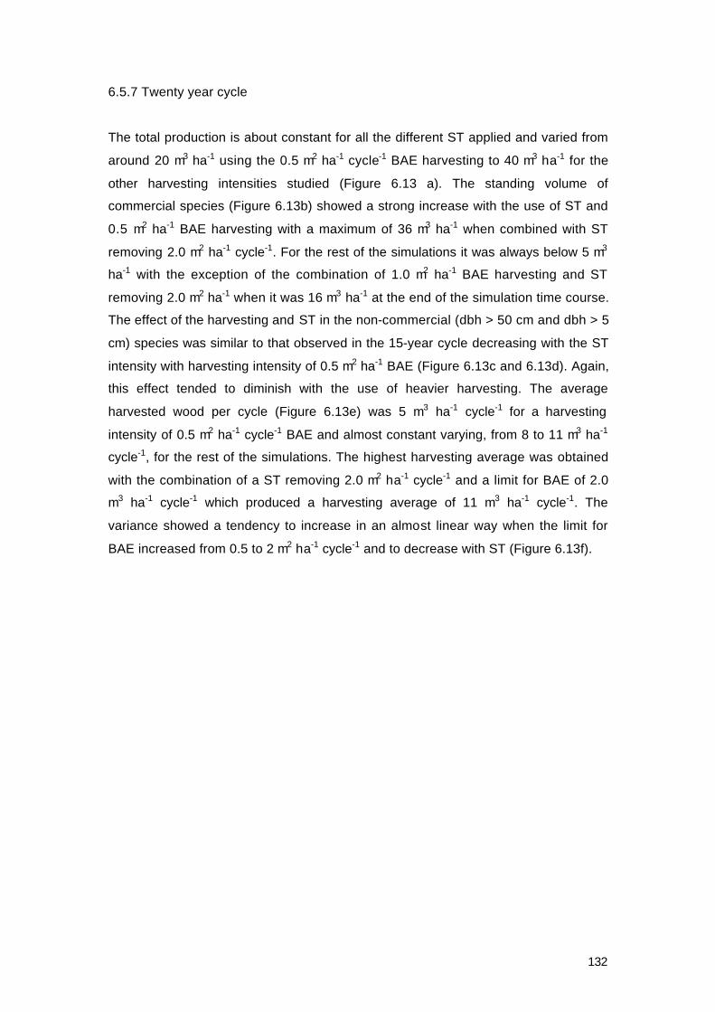
132
6.5.7 Twenty year cycle
The total production is about constant for all the different ST applied and varied from
around 20 m3 ha-1 using the 0.5 m2 ha-1 cycle-1 BAE harvesting to 40 m3 ha-1 for the
other harvesting intensities studied (Figure 6.13 a). The standing volume of
commercial species (Figure 6.13b) showed a strong increase with the use of ST and
0.5 m2 ha-1 BAE harvesting with a maximum of 36 m3 ha-1 when combined with ST
removing 2.0 m2 ha-1 cycle-1. For the rest of the simulations it was always below 5 m3
ha-1 with the exception of the combination of 1.0 m2 ha-1 BAE harvesting and ST
removing 2.0 m2 ha-1 when it was 16 m3 ha-1 at the end of the simulation time course.
The effect of the harvesting and ST in the non-commercial (dbh > 50 cm and dbh > 5
cm) species was similar to that observed in the 15-year cycle decreasing with the ST
intensity with harvesting intensity of 0.5 m2 ha-1 BAE (Figure 6.13c and 6.13d). Again,
this effect tended to diminish with the use of heavier harvesting. The average
harvested wood per cycle (Figure 6.13e) was 5 m3 ha-1 cycle-1 for a harvesting
intensity of 0.5 m2 ha-1 cycle-1 BAE and almost constant varying, from 8 to 11 m3 ha-1
cycle-1, for the rest of the simulations. The highest harvesting average was obtained
with the combination of a ST removing 2.0 m2 ha-1 cycle-1 and a limit for BAE of 2.0
m3 ha-1 cycle-1 which produced a harvesting average of 11 m3 ha-1 cycle-1. The
variance showed a tendency to increase in an almost linear way when the limit for
BAE increased from 0.5 to 2 m2 ha-1 cycle-1 and to decrease with ST (Figure 6.13f).

133
Figure 6.13: Twenty year cycle simulation components in a 70 years simulation course
with different harvesting intensities (basal area extracted) and Silvicultural treatments – ST
(no ST- white columns, ST removing 0.5 m2 ha-1 – grey columns, ST removing 1 m2 ha-1 –
white columns with diagonal lines; ST removing 1.5 m2 ha-1 white columns with crossed
lines and ST removing 2 m2 ha-1 – black columns): a- total harvested volume (m3 ha-1), b -
standing volume of commercial species dbh > 50 cm (m3 ha-1), c- standing volume of non-
commercial species dbh > 50 cm (m3 ha-1), d- total volume of non-commercial species e-
mean harvested volume per cycle (m3 ha-1) and f- coefficient of variation of the harvested
volume

134
6.6 Discussion
Sensitivity analysis
The model proved to be sensitive to both functions tested. The results from the
variation in mortality rates were apparent early during the simulation course because
of its direct influence on the tree population. This is in contrast with recruitment, which
represents small trees entering in the tree population contributing of small volume
around 0.2 to 0.4 m3 ha-1 yr-1. Thus it was to be expected that in the first 40 years of
the simulation course the difference among recruitment rates used had little effect
compared with the case of the mortality rates.
Mortality rates can be calculated directly which gives to this function a high
precision. However, recruitment rates are calculated through a regression between
stand basal area and the number of plants recruited in the period. It is to be expected
that sites with lower stand basal area should have a higher area of gaps that should
provide a better environment for the establishment of new recruits in the forest.
However, in this study, probably because of the short time of the measurements in the
permanent sample plots and also that the logging was a relatively recent event, the
inverse occurred and recruitment was higher where basal area was higher. A potential
problem with this function is that there is the possibility to have in a disturbed site a
high basal area (e.g. a logged area that possesses very big residual trees), and in the
same way in an undisturbed site (sites without natural or human disturbance) a closed
canopy and low basal area. In these situations the recruitment probably will be higher
in the site with the higher basal area than in the site with the lower basal area. The
same effect could be verified in the basal area increment, considering the above
described situation, a higher basal area increment could be expected in the site with
the higher basal area than in the other one.
The fact that the model produced reasonable outputs when running this set of
simulations with a relatively young and small data set, and that the functions
generated by two data sets (from CPATU and CPAF-ACRE) also produced (with
exception of recruitment function for the CPAF-ACRE data set) reasonable results,
are a good indication of its robustness. For the same reason is difficult to recognise
and point out its potential weaknesses. As other models, CAFOGROM requires a
large amount of data to produce good predictions, so that more information that is
accumulated from the past the better will be the vision of the future. In an evaluation of
the model’s performance comparing observed and estimated values over a period of
16 years (Alder and Silva, 1999), the system presented a tendency to overestimate

135
growth (e.g. for all species with diameter > 45 cm dbh the observed was 2.56 m3 ha-1
yr-1 and the estimated 3.13 m3 ha-1 yr-1)
Silvicultural treatments
For all forest management simulations tested, the volume produced over the 70-year
simulations using silvicultural treatments was greater than in the equivalent forest
management simulations without silvicultural treatments. In addition, the harvested
volume becomes more constant when silvicultural treatments are used. The managed
forest without silvicultural treatments, in all tested simulations, showed a sharp
decrease in the standing volume of commercial species at the end of the simulation
time course.
In short cycles the silvicultural treatments can cause a drastic reduction in the
population of non-commercial species > 50 cm dbh. In the simulations a sort of
equilibrium can be obtained between commercial and non-commercial species by
combining intensive ST with harvesting equal or superior to 1m2 ha-1 cycle-1 basal area
extracted.
Silvicultural treatments must be carried out very carefully to avoid the removal
of “potential” species, which could in future become commercial and a tree should be
eliminated only if it is directly competing with a more valuable one (Schmidt, 1987). In
this case it is important to note that the commercial species list was not changed
during the simulation (which is in fact very likely to happen in the real life). In addition,
when the system is designed for small farmers, some species (e.g. Ceiba spp) will not
be considered as commercial because of difficulties in the extraction of such large
logs and because of the low prices offered by the industry for collecting the logs in the
forest, but these species are commercial and some time in the future its use will be
possible by small farmers.
Harvesting rates (Basal area limit for extraction – BAE)
The limit for basal area (hence volume) extraction for cycles of 5 years cannot exceed
0.5 m2 ha-1. The other studied cycles obtained their peak production around 1.0 m2 ha-
1 and when the heaviest extractions were tested the standing commercial volume
decreased sharply and the system becomes unsustainable for wood production.
A light harvesting intensity combined with light ST usually resulted in a
treatment that promoted the non-commercial species, making the volume of these
species increase while the volume of commercial species decrease until near zero.

136
In short cycles of 5 and 10 years there were a general tendency for the
production to decrease when more intensive harvesting was applied due the total
extinction of the commercial species during the simulation time course. The other two
cycles presented an increase in the production when the harvesting intensity was
increased from 0.5 to 1.0 m2 ha-1 cycle-1 BAE, after that it showed a tendency to stay
constant. The cycles of 15 and 20 year harvesting intervals allowed the forest to grow
in a way which kept the production constant, despite the high variability among the
harvests. Probably better results can be obtained from these cycles but intermediate
ST must be applied to keep the forest productivity high.
Some harvests exceed the established limit for basal area extraction when the
harvesting limit was 0.5 and 1.0 m3 ha-1 cycle-1. It probably was because these low
harvesting rates did not allow big trees (with more than 0.5m2 of basal area which
means greater than 80 cm dbh) to cut. Thus, the program selected smaller trees for
harvesting, while they are available in the database, in a way to avoid exceeding the
determined limit for basal area extraction. However when these options finished
harvesting higher than the limit were observed sometimes increasing the total
production and always increasing the coefficient of variance. In practice this problem
can be avoided when the forester is taking the decision of which trees will be logged in
the compartment, by reducing the number of trees to be logged per hectare, hence
reducing the harvested volume and keeping some standing commercial volume for the
next harvest.
5 year cycles
Some reasonable simulations could be produced with a 5-yr cycle which gave regular
harvesting around 4 to 5 m3 ha-1 cycle-1. However these results were obtained through
a combination of low harvesting rates with intensive ST, resulting in a sharp decrease
in both the volume of commercial and non-commercial species. The reduction of the
commercial volume after harvesting is not a big problem and is even expected on
longer cycles, but for very short cycles some reserves must be present to guarantee
the following harvests. In addition, the variance was usually too high to be acceptable
(e.g. when harvesting is near zero in the cycle, the farmers receive no income).
Also, the low productivity and the greater area of the compartments increases
costs and labour demand and must be considered as strong economic limitation for
the use of 5 year cycles and, due the need for annual and regular incomes longer
cycles are recommended.

137
10 year cycle
Harvesting without the use of silvicultural treatments, even in the lowest intensity (0.5
m2 ha-1 cycle-1) promoted a decrease in the volume of commercial species in diameter
classes above 50 cm dbh and hence a decrease in the harvested volume in the later
cycles. The management without ST allow the maintenance of a high volume in the
forest but a low volume of commercial species, because the forest remain dominated
by non-commercial species.
The best results obtained were with the use of harvesting intensities from 0.5
to 1.0 m2 ha-1 cycle-1 allied with intense silvicultural treatments. Silvicultural treatments
removing 1.0 and 2.0 m2 ha-1 cycle-1 resulted in uniform harvests and allowed the
maintenance of the commercial volume after the last harvesting between 17 and 30
m3 ha-1. The intensive ST promoted a reduction in the volume of trees of non-
commercial species with dbh > 50 cm.
There is a strong response from the managed species when ST are applied
with 1.0 m2 ha-1 cycle-1 basal area extracted harvesting, but still a high decrease in the
volume of non-commercial species due the repetition of intensive ST. The use of
repeated ST is a decision which must be taken by the forester so that the
development of the forest keeps the productivity of the managed species high and at
the same time protecting the biodiversity and the potential species (Appendix 3).
Among all simulations, the forest management using a 10 yr-cycle, 1.0 m2 ha-1
BAE harvesting and ST removing 2.0 m2 ha-1 basal area, produced a high and uniform
harvests (from 8 m3 ha-1 to 10 m3 ha-1).
15 year cycle
Longer cycles demand more intensive harvesting rates as a way to compensate the
smaller number of harvests in the period. More intensive harvesting can produce
higher yields in the short-term, but the standing volume of commercial species has a
tendency to decrease sharply during the course of the simulation. For the 15-yr cycles
the need of a high standing commercial volume at the end of simulation is not as
important as for shorter cycles, because the forest will have more time to recover.
Thus a standing commercial volume from 10 to 20 m3 ha-1 at the end of the simulation
can be considered enough to guarantee the sustainability of the production.
The ST removing 1.0 m2 ha-1 cycle-1, produced similar results to the equivalent
simulation for 10 year cycle, but with lower total volume production over the course of
a 70 year simulation due a smaller number of harvests. With the heaviest silvicultural

138
treatments, removing 2.0 m2 ha-1 cycle-1 and a limit for BAE of 1.0 m2 ha-1 cycle-1, 15-yr
cycles obtained a total volume production around 50 m3 ha-1. In this case the variance
was low, and standing commercial volume at the end of the simulation was high,
around 30 m3 ha-1 and the harvests presented an average of 10 m3 ha-1 cycle-1. These
cycles can be considered for larger areas and a larger set of commercial species, but
the 10-yr. cycles are preferred from an economic point of view for the present
purpose.
20 year cycle
Twenty-yr. cycles are much more recommended for big areas and forest management
techniques involving the use of high technology for logging, skidding and processing
the wood.
The low response of the forest to ST probably has two main causes, the need
of an intermediate ST, for example around the 5th year after the forest exploitation,
and the low number of commercial species.
For this cycle length, the heaviest harvesting rates must to be applied to
compensate the smaller number of harvests. Higher harvesting rates produced
harvests about that which could be expected from a 20 year harvesting cycle, but only
in the two first cycles. After that the forest could no longer support the intervention and
both standing commercial volume and harvested volume fell to around zero. The final
volume of commercial species does not have the same importance which it has for
short cycles due the longer period which the forest has to recover. However, the
maintenance of the commercial volume around 10 to 20 m3 ha-1 will guarantee the
next cycle.
The decision whether to use longer cycles is related not only to ecological and
economic matters, but also to social and political aspects. The pressure for land
tenure in Amazon is becoming stronger and the risk that the forest may be used for
different activities in the intervals between cycles is considerable, and have been one
of the most common reasons for the failure of forest management in the tropics.

139
6.7 Conclusions
1- Without silvicultural treatment the total production is about constant in short cycles
(from 5 to 15 year cycles). The need for ST is due the small number of commercial
species competing with a large number of non-commercial or potential species. With a
larger set of commercial species the harvesting itself should produce the same effect
as ST, eliminating the need to use it. The low and about constant production
presented in the simulations without silvicultural treatments indicate the need to
provide competitive benefits to the managed species.
2- Strong silvicultural treatments (2.0 m2 ha-1) must be applied with care especially in
short cycles, because they are expensive, they affect negatively the population of
potential species (verified by the sharp decrease in volume of these species) and
increase the risks of biodiversity losses.
3- The variance increases when the extracted basal area increases, in all the studied
cycles with the exception of 5-yr cycles, in which the variance was always high. It
means that more intensive harvesting rates produce irregular harvests among cycles
due the absence of commercial species to be logged.
4- Ten-yr. cycles seem to be the best option for sustainable forest management in the
conditions presented in this work. Regular harvests from 8 to 10 m3 ha-1 cycle-1 can be
expected with the combination of a harvesting intensity around 1.0 m2 ha-1 cycle-1 and
ST removing around 2.0 m2 ha-1 cycle-1.
4- 20-yr. cycles are not applicable to small farms, because they demand much larger
areas. The alternative for use of these cycles in small farms should be a two-year
interval between harvesting, which is usually not suitable due the need for annual
incomes from the forest. In addition the total production (using the conditions of this
study) was below that of the short cycles, probably because of the need for more than
one ST (few species competing with a much larger population) and a larger set of
commercial species to allow more intensive harvesting rates. Alternatively, ST five
years after logging can be tried. The use of heavy machines (Skidders) must be
considered for these cycles for harvesting rates of 2 m2 ha-1 cycle-1 and above. Longer
cycles might be suitable for small properties where forest management is not
considered as a main activity, or where the calendar of activities other than forest
management has more economic importance or labour demand.
5- The results of the simulations must be interpreted as tendencies presented by the
forest for different interventions. In general, simulations have the tendency to produce
better predictions as time passes and the management system must be flexible
enough to assimilate the necessary changes. Thus the predictions produced by the

140
simulations are important for planning but they cannot replace the field experience of
the foresters. This is especially important in a scenario where the set of commercial
species is constantly changing, making delicate decisions such as which plants can
be removed as silvicultural treatment.
6- The improvement of the model performance demands more data. Additional
permanent sample will be established in the area in the year 2000.

141
CHAPTER 7
Summary and General Conclusions
7.1 Introduction
Despite pressure from conservationists and the efforts of most governments from
tropical countries, tropical forests are still being slashed and burned on a considerable
scale. The reason for this is usually that the land is needed to sustain the people who
live there and, although cattle breeding and shifting cultivation have a low profitability
in the tropics, there are no economic alternatives to these activities. The obvious
conclusion from this is that to preserve tropical forests it is necessary to give them a
value. As long as tropical forests are no more than an obstacle to the cultivation of
crops and pasture, all the possible arguments of conservationists such as biodiversity
protection, global warming, reduction in carbon emission and the protection of the
ozone layer, will not produce the desired effect of reducing deforestation rates.
Forest management has been tried, very often without success, in several
tropical countries. The most common reasons for its failure were the long felling cycles
required and the non-involvement of the local populations. As a result of this relatively
unsuccessful history, the concept of forest management has become misunderstood,
and what was actually a socio-economic problem (demographic pressure and the
need to produce food from the land) was interpreted as a technical problem (the
systems were not working because they were inadequate for the forests). It also gave
forest management the reputation for being the first step to deforestation and this
infamy has persisted until today being used frequently to demonstrate how
impracticable the management of tropical forest is (Poore, 1989; Dawkins and Philip,
1998).
Alternative traditional extractivism practices have been recommended (e.g.
Fearnside, 1989). However, because of the low density of the marketable species
(e.g. Hevea brasiliensis and Bertholletia excelsa), and the competition from
plantations, this activity is nowadays economically impracticable in Brazil (Homma,
1997). Agricultural techniques have been developed to improve traditional shifting
cultivation practices, the establishment of pastures (e.g. Valentim, 1989) and
agroforestry systems (e.g. Fernandez et al. 1999). All these techniques are indeed
very good, but alone they just emphasise the idea that the forest is an obstacle that
must be replaced, for the implementation of these alternative land uses.

142
This thesis had the aim of presenting a forest management system to be
applied on small farms, especially in the settlement projects of the Brazilian Amazon,
and to initiate the debate about its sustainability by investigating the responses of the
forest to the forest management interventions in terms of changes in natural
regeneration in the felling gaps and the dynamics of the residual trees. Using the
program CAFOGROM, an additional aim was to simulate the forest responses to
different cycle lengths, harvesting intensities and silvicultural treatments to determine
the theoretical optimum combination of these parameters for sustainable timber
production.
The reason to provide an alternative forest management system for small
farmers came from two main sources. First, the total population of Acre State is
483,593 inhabitants; 168,322 of them live in the countryside (IBGE, 1997). There are
around 20,000 families living in settlement projects in Acre (INCRA, 1998).
Considering that the average size of a family in Acre is around five people there is a
total number of 100,000 inhabitants or around 60 % of the population in rural areas.
These people are occupying an area of 1,5000,000 ha, which represents 10 % of the
total area of Acre State (152.598 km2) and a total area of legal forest reserves of
around 750,000 ha. So the potential problems which can arise from land use (e.g.
deforestation) in Acre State is strongly concentrated in settlement projects and small
properties.
Secondly, although the Brazilian forest code specifies the conservation of 50
% of the area of properties as forest cover in Amazon, the mean area deforested in
these farms in 1994 (PC Peixoto in Acre State and PC Theobroma in Rondônia State
(Witcover, 1994)) was 40 % of the total area, with a mean deforestation rate of 2.4 ha
yr-1. As the size of these farms is around 100 ha, and assuming the same
deforestation rate as 1994, this year (1999), on average, the farmers of settlement
projects in Acre and Rondônia States, are reaching the limit of 50 % of their properties
which they can legally slash and burn for shifting cultivation or pasture establishment.
Therefore it is likely that they will not stop, or even reduce, the deforestation rate on
their properties unless they can find an economic use for their forests.
7.2 The forest management system
The proposed forest management system was designed for small farmers and aimed
to generate a new source of family income whilst maintaining the structure and
biodiversity of the legal forest reserves. The expectation is that small-scale harvesting
can change the emphasis of production in Brazilian Amazon properties (by

143
incorporating a much broader range of legal forest reserves into the production
system) and create new models of rural development for the region.
There is a long history of forest exploitation in the Amazon based on traditional
‘low technology’ methods. These methods require low inputs and have a relatively
benign environmental impact, but production and profit margins are also low (Oliveira
1989). The extraction of timber by small producers is a seasonal activity. This permits
them to continue other essential activities (hunting, fishing, non-timber product
extractivism and subsistence agriculture).
The proposed model is a formalisation of these traditional methods. It is a
policyclic forest management system similar to the traditional selection system
(Jonkers, 1987). Selective logging in many respects creates disturbances akin to
natural tree falls and results in canopy openings that stimulate the growth of advance
regeneration (Uhl et al. 1990). I suggest that low-impact disturbance at short intervals,
combined with silvicultural treatments, will create a gap mosaic of different ages and
permit the maintenance of a forest with a similar structure and biodiversity to that of
the original natural forest, and that canopy openings will allow young trees to grow
faster. The short rotation cycle substitutes the larger impact caused by heavier
interventions distributing it over time. The property’s legal forest reserve area (50 % of
the total area) was considered as the production unit for the implementation of forest
management. The number of annual harvesting coupes was determined on the basis
of a minimum felling cycle of ten years and an annual harvest of 5-10 m3 of timber per
hectare, through the following sequence of operations for the evaluation of the
production capacity of the forest, planning of exploitation activities, and monitoring.
- Forest inventory, 1 - 2 years before harvesting. The inventory determines the
potential of the forest for forest management and the length of the cutting
cycle.
- Compartmentalisation and permanent sample plot establishment.
- 100 % prospective inventory of trees > 50 cm dbh and tree mapping.
- Preparation of the exploitation plan, marking trees for felling and
establishment and measurement of permanent sample plots for growth and
yield studies one year before logging.
- Species selection and felling rate determination based on the species
diameter distribution, growth rates and seed dispersal.
- Logging, observing directional felling wherever possible. A logging intensity of
5-10 m3 ha-1 and felling diameter limit of 50 cm dbh should be observed.
- Artificial regeneration of commercial species in the felling gaps if necessary,
immediately after logging.

144
- Measurement of the PSPs one year after logging to estimate logging damage
and stocking of the residual stand.
- Measurement of the PSPs three years after logging.
- Measurement of the PSPs five years after logging.
- Refinement to assist growth of the residual commercial trees and artificial
regeneration of noble species if necessary.
- Measurement of the PSPs 10 years after logging.
- Redefinition of the cutting cycle, cutting rate and silvicultural treatments
according to data provided by the PSPs before the beginning of the next cycle
(ten years).
The system is new in three main characteristics: the use of short cycles in the
management of tropical forest, the low harvesting intensity and environmental impact
and the direct involvement of the local population in all forest management activities.
From the previous experience with forest management, even though it is
known that the short cycle can provide for continuing benefits of enhanced growth in
the residual trees, it is expected that additional silvicultural treatments will be
necessary between harvests to maintain forest productivity at a high level (e.g. De
Graaf, 1986). The application of silvicultural treatments will be facilitated by the fact
that small farmers regularly enter or cross the management area during the working
day for hunting, fishing and rubber tree tapping. The silvicultural treatments that have
been applied already, such liana cutting and directional felling were effective at
reducing the damage promoted by the logging and to protect the residual trees of
commercial and potential species.
The harvesting intensity proposed is a reasonable first approximation. It
allowed the maintenance of populations of the managed species and a considerable
income for the farmers. However, in the future, with more information about forest
dynamics and the entrance of some of the potential species onto the timber markets,
more intensive harvesting could be applied to maximise forest use. The price of the
timber is likely to increase in the future because of the rise in the demand for tropical
timber worldwide and the restriction in supply, especially of the more valuable timbers
(e.g. Mahogany). Therefore the current standing stock of timber represents an
investment rather like a savings account. This may be true even for stems of species
that are not highly valued at present, because new species become marketable over
time.
The conversion of the logs to planks was the most expensive, labour
demanding and probably also the most dangerous operation, although the conversion

145
yields of around 50 % were above expectation. The project has received some
support from the ASB (Alternatives to Slash and Burn project), which involved the
acquisition of a one-man sawmill. This is a portable sawmill that can be transported to
the felling gaps. The expectation is that with the use of this equipment the conversion
of the logs will become easier and cheaper, and that not only will the yields increase
but also the quality of the final product will increase.
The use of the “zorra” over distances in the forest reduced the productivity of
the skidding phase. The alternative use of a wagon pulled by one ox to skid the planks
from the main skid trail to the border of the secondary roads, was successfully applied
this year, limiting the skidding by the “zorra” from the felled tree to the main skid trail
or a maximum distance of 200 m. This combination of methods made this phase
easier for both man and ox.
The short period of time the forest management system has been applied in
PC Peixoto (from 1996 to 1999) prevents definitive conclusions and it is possible that
in a few years some modifications might be necessary. In this sense, possibly the
greatest advantage of the short cycles is the flexibility to change interventions such as
harvesting intensity, silvicultural treatment, cycle length, the set of managed species,
etc. over a relatively short time scale and to adjust the system when necessary.
7.3 Natural regeneration
Artificial gaps
The higher diversity of seedlings in small and medium gaps than in the forest
understorey in the second year confirmed the expectation of higher species diversity
in the gaps. It is likely that diversity will continue to increase in the gaps, although
slower in gaps larger than 1000 m2 or with canopy openness greater than 25 %.
The increase in the relative density of pioneer species with increasing gap size
and canopy openness supports the work of Barton (1984) who showed that pioneer
species density is higher in larger gaps, but no evidence could be found for the
hypothesis that pioneer species regenerate more effectively in the gap centre and
shade-tolerant species in the gap edges. However, there was a significant difference
in the relative density of the pioneer species in the gap border and in the gap centre at
this site. There was also a tendency for the relative density of pioneer species to
decrease in the smaller gaps and to increase in the larger ones from the first to the
second year after gap creation.

146
Differences in gap size and canopy openness produced significant differences
in the growth rates of seedlings, but no statistically significant differences could be
determined according to the position of the quadrats in the gaps. Mortality rates
increased with gap size and recruitment rates decreased. One possible interpretation
for the low recruitment in the larger gaps could be because of the high mortality there,
the potential recruit (seedlings which could reach 1 m in height during the period
between the census) died between the first and the last measurement. It also can be
interpreted as an effect of the short time of the measurement and the natural tendency
is that the larger gaps will be filled in the future and a higher seedling density is
expected in these gaps.
The density and recruitment of seedlings of commercial species was not
different between gap sizes, but gap creation increased the growth rate of the
seedlings of these species.
Felling gaps
The gaps produced by logging in PC Peixoto can be classified as small or less often
medium sized (canopy openness from 10 % to 25 %). The richness and diversity of
seedlings in these areas one year before logging and two years after logging were
similar. The logging produced a sharp decrease in the richness and diversity of both
gap zone areas, but two years after logging they were similar to the understorey
forest. It is probable that diversity will become higher in the crown zone than in the
natural forest understorey over time. The relative density of pioneers, two years after
logging, was similar in both gap zones at around 35 %, which is also similar to that
observed in the small gaps in the artificial gaps experiment.
The low growth rate of seedlings in the felling gaps might be associated with
the low canopy openness in the trunk zone, and the intense competition from the
seedlings that survived the logging as well as the felled tree crowns acting as a
barrier, in the crown zone.
Mortality of seedlings in the gap zones decreased significantly from the first to
the second year and did not differ significantly from that in the understorey. In the
trunk zone, felling the tree, conversion of the logs to planks and skidding the planks
resulted in complete mortality. In addition, the residues of the logs interfered with the
germination of seeds (personal observation) and reduced the recruitment of new
seedlings.
The felling gaps do not affect the density and recruitment of commercial
species, and again a significant increment in growth rates was observed. Small and

147
medium gaps, or gaps with less than 25 % canopy openness resulted in improved
regeneration from the forest management point of view, with fewer pioneer plants
higher species diversity and lower mortality, although the growth rates in the two first
years was significantly lower than in the larger gaps.
Consequences and recommendations for the management system
In general the results from the artificial gaps experiments also support Hawthorne
(1993) who found that larger gaps are undesirable for almost every reason except the
convenience of the loggers. Therefore regulations must be applied to limit the total
number of trees felled in a compartment, as well as the number of adjacent trees
which can be felled, so that gap sizes will be small.
Most of the gaps produced by the felling of trees in Pedro Peixoto Colonisation
Project can be classified as small (considering the categories used in this study).
Small and medium gaps in the artificial gap experiment showed the optimum results
for natural regeneration from the perspective of forest management. Despite some
differences arising during the creation of artificial gaps (destruction of the original
seedling community and removal of large branches) and felling gaps, the
environmental conditions (e.g. temperature, humidity and water availability) were
similar. Thus, the continuation of the study in both conditions (artificial and felling
gaps) will probably emphasise these similarities. Studies of artificial gaps have the
advantage of controlling important characteristics of gaps, such as size, topographic
position and orientation and they are a tool to help forecast regeneration dynamics in
the felling gaps where the control of such characteristics are usually difficult.
The distribution of the impacts in space and time as proposed by the studied
silvicultural system coincides, with these principles. The low harvesting rates and
short cycles used reduces the number of gaps and distributes the impacts among the
following harvesting cycles, in contrast to what happens with conventional forest
management where the impacts occur at one time. In addition, the potential benefits
of canopy opening are repeated at shorter intervals, which avoids stagnation of forest
production. The felling of the trees in the compartments produced gaps which could
be classified as small gaps in the artificial gaps experiment. The fact that all seedlings
were removed during the creation of artificial gaps can be used to explain differences
in growth rates and recruitment in the first two years. However, the species
composition, richness and diversity of seedling communities were similar.
More frequent logging has the disadvantage of producing more damage to the
residual trees. Special care must be taken during the harvesting operations, through

148
the use of directional felling and liana cutting. In addition, the extraction of the logs by
animal traction significantly reduces this damage.
7.4 Forest dynamics
The mean periodic annual diameter increment (0.28 cm yr-1) was similar to that found
by other work in the tropics. Differences in crown exposure produced a highly
significant effect on the growth of the trees. The sub-groups of species also possess
different growth rates, probably because of different growth patterns shown by those
species (e.g. Bertholletia excelsa – big pioneers and Gustavia augusta – understorey
species). The increase in diameter increment from small trees to big trees is also
correlated with increase in crown exposure and growth patterns. The influence of
management was positive in terms of diameter increment increase in both
mechanised and non-mechanised logging. Diameter increment immediately after
logging in PC Peixoto was slower than in the undisturbed forest possibly because the
short time between logging and measurement did not allow the effect of canopy
openness to be observed.
Mortality rates in the natural forest were similar to other studies in tropical
forests i.e. between 1 % and 2 % yr-1. The higher mortality recorded at the last
measurement (1999), can be a consequence of higher occurrence of winds and
storms in this period ("El Niño" event). Although mortality caused by mechanised
management was underestimated, it is still higher than in the natural forest.
Recruitment in the areas managed by the farmers in PC Peixoto (using non-
mechanised methods), was not significantly higher than in the natural forest probably
because the canopy opening caused by the harvesting operations was minimised by
the low harvesting intensity. However, as recruitment considered plants with dbh
greater than 5 cm, the period covered by the study was not enough to include some of
the plants that germinated after the logging. Thus, an increase in the recruitment rates
in those areas may be expected in the next few years.
The increase in the damage from natural causes from the first to the last
measurement might be associated with the logging, but it is also possible that 1998
was an atypical year, with more frequent strong storms in the area.
The difference in species richness and diversity in the low impact management
system before and after logging was low, and it is probable that before the end of the
cycle diversity will increase in this area. The high impact management system, at least
in the short-term, produced a high variation in the composition of the forest, but the
density of commercial species did not change.

149
An acceptable volume increment of commercial species was compatible with
the logging intensity and cycle length proposed for both forest management systems
examined. The high volume increment of commercial species might be an effect of the
practice of the directional felling, protecting residual trees of commercial and potential
species.
7.5 The simulations
Sensitivity analysis and the weakness and limitation of the application of the model in
this study
The model was demonstrated, when tested, to be sensible for both recruitment and
mortality. This is important in the sense that the precision of the predictions come from
the capacity of the model to show in their outputs the difference caused by small
changes in the forest dynamics (Pinard, 1993). Functions generated from the data
from CPATU were compared with those using the data set of the permanent sample
plots in CPAF-ACRE and in Pedro Peixoto Colonisation Project. Although generated
in different regions of Amazon, these two forests have similar characteristics in terms
of climate (temperatures around 250 C, rainfall around 2000 mm yr-1, mean relative
humidity over 80 % and a not very pronounced dry season concentrated between
August and September), geographical position (from 20 to 60 S), soil (dystrophic
yellow latosol), forest structure (terra-firme forest, with emergent species such as
Bertholletia excelsa and Couratari sp. and basal area around 25 to 30 m2 ha-1) and
forest dynamics (mortality rates in the undisturbed forest around 2 % year-1 and mean
diameter increment around 0.25 cm year-1). All data from Tapajós National Forest are
in Silva (1989); Silva et al. (1989); Silva et al. (1996) and for PC Peixoto and CPAF-
ACRE in this work (Chapter 2 (site description), Chapter 3 (forest inventory results)
and Chapter 5). Thus, the use of the functions generated by the CPATU data set is a
reasonable approach to parameterising the functions generated by the CPAF-ACRE
data. In general the functions generated with my data set produced realistic outputs
and the differences from those using CPATU data (e.g. logging damage, mortality
rates and diameter increment) were expected as a result of the different management
techniques and harvesting intensities applied for these two sites. These differences
also emphasises the need for the development of different functions for the proposed
forest management system.
The unexpected equation generated for recruitment probably arose because
the recruitment in the managed areas was low. Thus, because of the lack of

150
recruitment in the managed areas, which presumably have a lower basal area than
the undisturbed areas, the regression showed a tendency for recruitment to increase
with basal area. The natural tendency is that these areas will have a higher
recruitment in future years and the basic assumption of the recruitment function, that
sites with lower basal areas will have a higher probability of higher recruitment, is
correct.
In addition there is a possibility for a disturbed site to have a high basal area
(e.g. a logged area that possesses very big residual trees), and for an undisturbed site
(sites without natural or human disturbance) to have a closed canopy and low basal
area. In these situations the recruitment will probably be higher in the site with the
higher basal area than in the site with the lower basal area. The same effect might be
found for basal area increment, considering the situation described above whereby, a
higher basal area increment is expected in the site with the higher basal area than in
the other one.
A similar effect for recruitment was observed in the artificial gaps, probably
associated with climatic conditions during the period of this study. Larger gaps, which
in a forest management condition could be associated with higher harvesting
intensities and as consequence lower basal areas, showed lower recruitment rates.
On the other side, the growth of the residual tree, in terms of stand basal area, was
according to the assumption of the model and the managed areas showed higher
basal area increment in the studied period.
However, it must be pointed out that the data available in CPAF-ACRE for this
work is not robust and better predictions are expected in the future from the new
permanent sample plots already established in new areas where the proposed forest
management system was implemented in 1998 (Antimari Forest, FUNTAC, 1989).
Silvicultural treatments
Without silvicultural treatment, total production is almost constant in short felling
cycles (i.e. from 5 to 15 years). The need for silvicultural treatments is due to the small
number of commercial species competing with a large number of non-commercial or
potential species. With a larger set of commercial species, higher harvesting intensity
could be practised and the harvesting itself should produce the same effect as
silvicultural treatments, eliminating the need to use them. On the other hand, heavy
silvicultural treatments must be applied with care because they can affect negatively
the population of potential species and increase the risks of biodiversity loss.

151
Cycle length, harvesting intensity and timber production
The variance in the average harvested volume increased when the harvesting
intensity increased in all the cycles examined, this suggests that heavy harvesting
might result in the extinction of commercial species, or a lowering their density if more
intensive silvicultural treatments are applied.
Five year cycles always showed a high variance in the harvested timber per
cycle. The high final production values obtained in some simulations resulted from a
combination of low harvesting rates with intensive silvicultural treatments, resulting in
a sharp decrease in the standing volume of the forest as a whole. The reduction in the
commercial volume after harvesting is not a major problem, and is even expected on
longer cycles, but for very short cycles some residual trees of commercial species
must be present to guarantee the following harvests. In addition, the low productivity
and the greater area of the compartments increases costs and labour demand, and
must be considered as strong economic limitations on the use of five year cycles.
Therefore, because of the need for annual and regular incomes, longer cycles are
recommended.
Twenty and 15 year cycles are not applicable on small farms, because they
demand much larger areas to be economically viable. In addition, the total production
(using the conditions of this study) was less than in the short cycles. The lower
production is caused by the need for more than one silvicultural treatment and a larger
set of commercial species to allow more intensive harvesting rates.
Ten year cycles are the most appropriate compromise for sustainable forest
management under the conditions examined in this study. A regular harvesting of 8 to
10 m3 ha-1 cycle-1 can be expected with the combination of a harvesting intensity of
around 1.0 m2 ha-1 cycle-1 and silvicultural treatments removing around 1.5 m2 ha-1
cycle-1.
Implications for the forest management system
The results of the simulations must be interpreted as qualitative responses of
presented by the forest to different interventions. Thus, the predictions produced by
the simulations are important for planning but they cannot replace the field experience
of foresters. This qualification is especially important in a scenario where the set of
commercial species is constantly changing, resulting in delicate decisions such as
which trees can be removed during silvicultural treatments.

152
The initial choice of ten year cycles and harvesting rates of around 10 m3 ha-1
cycle-1 were consistent with the results of the simulations. There is a clear need for
silvicultural treatments to increase forest production. In the forest dynamics study, it
was observed that the changes in the crown illumination status of the trees produced
an increase in their growth rates, therefore it is reasonable to apply a competitive
advantage to a particular group of species being affected by the forest management.
The model will be also a tool to simulate different forest management
scenarios during harvesting intervals, not only using new data from the forest
dynamics studies but also variations in the set of commercial species during this
period.
7.6 The way ahead: constraints, opportunities and future research
The project will continue as a part of the EMBRAPA research programme. Additional
support has been provided by the ASB (alternative to slash and burn) project that has
PC Pedro Peixoto as one of its chosen sites for research. In addition the project was
submitted to the “Pro-manejo” project which is administered by the Brazilian Institute
of Environment and Natural Resources (IBAMA) and supported by the G-7 Nations
and the GTZ. This project aims to identify and to give support for the implementation
of “promising initiatives” for forest management in the Amazon. The continuation of
the project will allow the continuation of research on forest dynamics and plant
succession in the felling and artificial gaps, which demand long term studies
(Whitmore and Brown, 1996).
The system is also being implemented in the Antimari forest management
project. This project has the aim of sustainable timber and non-timber production and
research. It has the support of ITTO and is being conducted by FUNTAC (Acre State
Technology Foundation). Fifteen permanent sample plots have already been
established there and all the studies will be conducted through a partnership between
EMBRAPA and FUNTAC teams.
Some opportunities have been created for the implementation of forest
management for small farmers in the Amazon. A specific legislative framework
covering implementation and inspection of management plans on small properties
was approved in 1998, establishing the use of short cycles and animal traction by
IBAMA (Brazilian Institute for Environment and Natural Resources) agencies. In
addition, BASA (the Amazonian Bank) has implemented a scheme that allows farmers
access to a specific account to finance forest management following this model.

153
Some outstanding problems must still be solved, such as the lack of control of
the trade in illegal timber, and the entrance onto the market of royalty-free timber from
areas being converted from forests to agriculture. These problems make it difficult for
legally produced timber to compete on an equal basis. In addition, the extension
services that already exist in Brazil (EMATER) are only for technical support in
activities related to agriculture. They cannot act in the same way for forest
management activities. Their support will be necessary in the future to help the small
farmers with technical activities such as prospective forest inventories and harvesting
intensity determination, tasks which are now being performed by CPAF-ACRE.
The wide application of the system proposed here in tropical forests will be
limited by the size of the properties. The size of the small farms in the Brazilian
Amazon (from 80 to 100 ha) are, very probably, an exception in the world and the
forest management proposed in this thesis will not be applicable to forest areas much
smaller than 40 ha.
In general, new activities and technologies are difficult to implement, especially
in a complex socio-economic and ecological environment. However, there is a need
for economic and ecologically sound technologies to be implemented in the Amazon
and the small scale forest management proposed in this thesis has been
demonstrated to be viable in these respects.

154
BIBLIOGRAPHY
ABDUL, K.R., WAN RAZALI, W.M., SHAHRULZAMAN, I. and AZMAN, H. 1992.
Growth response of hill dipterocarp forest following two methods of logging in
Peninsular Malaysia. In: Proceedings of the Symposium on Harvesting and
Silviculture for Sustainable Forestry in the Tropics. Kuala Lumpur, Malaysia, pp.
24-31.
ADLARD, P.G., SPILSBURY, M.J. and WHITMORE, T.C. 1989. Current thinking on
modelling the tropical moist forest. In: Mohd, W.R.W., Chan, H.T. and Appanah,
S. (Eds.) Proceedings of the Seminar on Growth and Yield in Tropical
Mixed/moist Forest. Forest Research Institute, Malaysia, pp. 6-20.
AGYEMAN, V.K., SWAINE, M.D., THOMPSON, J. Responses of tropical tree
seedlings to irradiance and the derivation of a light response index. Journal of
Ecology, 87: 815-827.
ALDER, D. 1990. GHAFOSIM: A projection system for natural forest growth and yield
in Ghana. Consultancy report to Ministry of Lands and Natural Resources.
Ghana, 144 p.
ALDER, D. 1995a. The preliminary development of the CAFOGROM forest growth
model. ODA/CPATU. Silviculture research Project, Brazil. Internal Consultancy
Report, 28 p.
ALDER, D. 1995b. Growth Modelling for Mixed Tropical Forests. Tropical Forestry
Papers No. 30. Oxford Forestry Institute, Oxford, U.K. 231p.
ALDER, D. 1996a. Further development of growth modelling techniques for
Amazonian selection forest management. Report of a consultancy to CPATU.
Belém, Brasil 17 p.
ALDER, D. 1996b. CAFOGROM.XLS: A simulation model for natural forest
management: User's guide and technical reference manual. U.K. Overseas
development Administration. Oxford, 40 p.
ALDER, D. and SILVA, J.N.M. 1999. An empirical model for management of terra-
firme forest in the Brazilian Amazon. Forest Ecology and Management, in press.
ALMEIDA, S.S. 1989. Clareiras Naturais na Amazônia Central: Abundância, estrutura
e aspectos da colonização vegetal. MSc thesis, unpublished. INPA/FUA. Manaus,
Brasil, 102 p.
APPANAH, S., WEINLAND, G., BOSSEL, H. and KRIEGER, H. 1990. Are tropical rain
forests non-renewable? An enquiry through modelling. Journal of Tropical Forest
Science, 2(4): 331-348.

155
ARRIAGA, L. 1988. Gaps dynamic of a tropical cloud forest in North-eastern Mexico.
Biotropica, 20(3): 178-184.
BARROS, A.C. and UHL, C. 1995. Logging along the Amazon river and estuary:
patterns, problems and potential. Forest Ecology and Management, 77: 87-105.
BARTON, A.M. 1984. Neotropical pioneer and shade tolerant tree species: do they
partition treefall gaps? Tropical Ecology, 25: 196-202.
BARTON, A.M., FETCHER, N. & REDHEAD, S. 1989. The relationship between
treefall gap size and light flux in a Neotropical rain forest in Costa Rica. Journal of
Tropical Ecology, 5:437-439.
BATOUM, T. and NKIE, M. 1998. People in Forest Management. Tropical Forest
Update, 8(1): 11-13.
BAZZAZ, F.A. 1979. The physiological ecology of plant succession. Ann. Rev. Ecol.
Syst., 10: 351-371.
BAZZAZ, F.A. and PICKETT, S.T.A. 1980. Physiological ecology of tropical
succession: a comparative review. Ann. Rev. Ecol. Syst., 11: 287-310.
BLATE, G. 1997. Sustainable Forest Management in Brazil. Tropical Forest Update,
7(3): 14-15.
BORMAN, F.H. and LIKENS, G.E. 1979. Development of vegetation after clear
cutting: species strategy and plant community dynamics. In: Pattern and Process
in a Forested Ecosystem: Disturbance, Development and Stead State, Based on
the Hubbard Brook Ecosystem Study. pp. 101-137.
BOSCOLO, M. and BUONGIORNO, J. 1997. Managing a tropical rainforest for timber,
carbon storage and tree diversity. Commonwealth Forestry Review, 76(4): 246-
253.
BOSSEL, H., BRUENIG, E. F. and HUANG,Y.W. 1989. Tropical rainforest ecosystem
structure, functions and dynamics: the state of system analysis and modelling of
structural change and growth in CERP and ASEAC. In: Mohd, W.R.W., Chan,
H.T. and Appanah, S. (Eds.) Proceedings of the Seminar on Growth and Yield in
Tropical Mixed/moist Forest. Forest Research Institute, Malaysia, pp. 35-50.
BOUCHER, D.H, VANDERMEER, J.H., MALLONA, M.A., ZAMORRA, N. and
PERFECTO, I. 1994. Resistance and resilience in a directly regenerating
rainforest: Nicaragua trees of Volchysiaceae after hurricane Joan. Forest Ecology
and Management, 69: 123-144.
BRANDANI, A., HEARTSHORN, G.S. and ORIANS, G.H. 1988. Internal heterogeneity
of gaps and species richness in Costa Rica tropical wet forest. Journal of Tropical
Ecology, 4: 99-119.

156
BRAZ, E.M. and OLIVEIRA, M.V.N.d’. 1994. Manejo florestal para áreas com
populações tradicionais. In: III Simpósio Internacional de Estudos Ambientais
sobre Ecossistemas Florestais. BIOSFERA. Porto Alegre, Brasil, pp. 39-40.
BRAZ, E.M. and OLIVEIRA, M.V.N. d’. 1995. Arraste em floresta tropical: análise para
a identificação dos parâmetros ideais. In: II Simpósio Brasileiro sobre Colheita e
Transporte Florestal. Salvador, Brasil, pp. 222-237.
BRAZ, E. M. and OLIVEIRA, M. V. N. d’. 1996a. Plano de Manejo de Uso Múltiplo da
Floresta Estadual do Antimari, Acre. In: IV Simpósio Internacional sobre
Ecossistemas Florestais. BIOSFERA. Belo Horizonte, Brasil, pp. 272-274.
BRAZ, E.M. and OLIVEIRA, M.V.N.d’. 1996b. Planning to reduce damage. Tropical
Forest Update, 6(3): 13-14.
BROKAW, N.V.L. 1982. The definition of treefall gap and its effect on measures of
forest dynamics. Biotropica, 14(2):158-160.
BROKAW, N.V.L. 1982. Treefalls: frequency, timing and consequences. In: Rand,
A.S. & Windsor, D.M (Eds.). The ecology of a tropical forest: seasonal rhythms
and long-term changes. Smith. Inst. Press. Washington, D.C. USA, pp. 101-109.
BROKAW, N.V.L. 1985a. Gap-phase regeneration in a tropical forest. Ecology,
66(3):682-687.
BROKAW, N.V.L. 1985b. Treefalls, regrowth, and community structure in tropical
forest. In: Picket, S.T.A. & White, P.S. (Eds.) The ecology of natural disturbance
and path dynamics. Academic Press. N.Y., USA, pp. 53-69.
BROKAW, N.V.L. 1989. Species composition in gaps and structure of a tropical forest.
Ecology 70(3): 538-541.
BROWN, N. and WHITMORE, T.C. 1992. Do dipterocarp seedlings really partition
tropical rain forest gaps? Phil. Trans. R. Soc. Lond. B., 335: 369-378.
BROWN, N. 1993. The implications of climate and gap microclimate for seedling
growth conditions in a Bornean lowland rain forest. Journal of Tropical Ecology,
9:153-168.
BROWN, N. 1996. A gradient of seedling growth from the centre of tropical rain forest
canopy gap. Forest Ecology and Management, 82: 239-244.
BRUCE, R.W. 1989. Log supply in Amazonas State Brazil, availability and constraints
to utilisation. Report prepared to the International Tropical Timber Organisation,
Yokohama, Japan. 17p.
BUDOWSKI, G. 1955. Distribution of tropical American rain forest species in the light
successional process. Turrialba, 15: 40-42

157
BURSLEM, D.F.R.P., ALDER, D. and WHITMORE T.C. 1996. COSSI, a cohort
simulation model of forest growth and yield in the Salomon Islands. O.F.I.
Occasional papers 50, 64p.
CANHAM, C.D., DENSLOW, J.S., PLATT, W.J, RUNKLE, J.R., SPIES, T.A. and
WHITE, P.S.. 1987. Light regimes beneath closed canopies and tree-fall gaps in
temperate and tropical forests. In: Canopy gaps in forest ecosystems. Ohio State
University, Columbus, Ohio, pp. 620-631.
CANHAM, C.D., DENSLOW, J.S., PLATT, W.J., RUNKLE, J.R., SPIES, T.A. AND
WHITE, P.S. 1990. Light regimes beneath closed canopies and tree-fall gaps in
temperate and tropical forests. Canadian Journal of Forestry Research 20: 620-
631.
CANNON, C.H., PEART, D.R., LEIGHTON, M. and KARTAWINATA, K. 1994. The
structure of lowland rainforest after selective logging in West Kalimantan,
Indonesia. Forest Ecology and Management, 67: 49-68.
CASTAÑEDA, A., CARRERA, F. and FLORES, J. 1995. Extraccion con bueyes y
aserrio con motosierra de marco: una alternativa para el manejo florestal
comunitario. Estudios de caso en el Adi “La Lupe”, Rio San Juan, Nicaragua.
Universidad Centro Americana - Proyecto Tropico Umido (UCA/SAREC), 27 p.
CAVALCANTI, T.J. da S. 1994. Colonização no Acre: uma análise socio-econômica
do projeto de assentamento dirigido Pedro Peixoto. Tese de Mestrado, não
publicada. Universidade Federal do Ceará - Centro de Ciências Agrárias.
Fortaleza, Brasil, 196p.
CHAI, D.N.P. and UDARBE, M.P. 1977. The effectiveness of current silvicultural
practice in Sabah. The Malaysian Forester. 40 (1): 27-35.
CHAI, F.Y.C. and SIA P.C. 1989. Stand table projections for a mixed swamp forest of
Sarawak. Proceedings of the Seminar on Growth and Yield in Tropical
Mixed/moist Forest. Forest Research Institute, Malaysia, pp 60- 77.
CHAI, F.Y.C. and Le MAY, V.M. 1993. Development and testing of diameter
increment models for mixed swamp forests of Sarawak. Forest Ecology and
Management, 58: 51-64.
CHANDRASHEKARA, U.M. & RAMAKRISHNAN, P.S. 1994. Successional patterns
and gap phase dynamics of a humid tropical forest of the Western Ghats of
Kerala, India: ground vegetation, biomass, productivity and nutrient cycling.
Forest Ecology and Management, 70: 23-40.
CHEAH, L C. 1978. Forest regeneration and development options in Peninsular
Malaysia today. Malaysian Forester, 41(2): 171-175.

158
CHIEW, K.Y. and GARCIA, A. 1989. Growth and yield studies in the Yayasan Sabah
forest concession area. In: Mohd, W.R.W., Chan, H.T. and Appanah, S. (Eds.)
Proceedings of the Seminar on Growth and Yield in Tropical Mixed/moist Forest.
Forest Research Institute , Malaysia, pp. 192-205.
CLARK, D.B. and CLARK, D.A. 1996. Abundance, growth and mortality of very large
trees in neotropical lowland rain forest. Forest Ecology and Management, 80:
235-244.
CONDIT, R., HUBBELL, S.P. and FOSTER, R.B. 1995. Demography and harvest
potential of Latin American timber species: data from a large permanent plot in
Panama. Journal of Tropical Forest Science, 7(4): 599-622.
CONDIT, R., HUBBELL, S.P., La FRANKIE, J.V., SUKUMAR, R., MANOKARAN, N.,
FOSTER, R.B.F. and ASHTON, P.S. 1996. Species-area and species-individual
relationships for tropical trees: a comparison of three 50-ha plots. Journal of
Ecology, 84: 549-562.
CONDIT, R., FOSTER, R.B.F., HUBBELL, S.P., SUKUMAR, R., LEIGH, E.G.,
MANOKARAN, N., LAO, S.L., La FRANKIE, J.V. and ASHTON, P.S. 1998.
Assessing forest diversity on small plots: calibration using species-individual
curves from 50-ha plots. In: Dallmeier, F and Comiskey J A. (Eds.) Forest
biodiversity research, monitoring and modelling, Man and the Biosphere series
vol. 14. UNESCO, Paris.
COSTA FILHO, P.P. 1991. Mechanised logging and the damages caused to tropical
forests: the case of the Brazilian Amazon. Paper presented at the X World
Forestry Congress. Paris, France.
DAWKINS, H.C. and PHILIP, M.S. 1998. Tropical Moist Forest Silviculture and
Management: a History of Success and Failure. CAB International, Wallingford,
359 p.
DE GRAAF,N.R. 1986. A silvicultural system for natural regeneration of tropical rain
forest in Suriname. Agricultural University, Wageningen, The Netherlands. 250 p.
DE GRAAF, N.R. and ROMPAEY, van R. 1990 The CELOS experiments on
silviculture with natural regeneration in Suriname. Em: Anais de le “Atelier sur
l’amenagement et la conservation de l’ecosysteme forestier tropical humide”
Cayena, Guyane.
DE GRAAF, N.R. and POELS, R.L.H. 1990. The Celos Management System: A
Polycycle Method for Sustainable Timber Production in South America Rain
Forest. In: Anderson, A. (Ed.). Alternatives to Deforestation in Amazon. New York
Columbia University Press. pp 116-127.

159
DENSLOW, J.S. 1980. Gap partitioning among rainforest trees. Biotropica, 12(suppl.):
47-55.
DENSLOW, J. S., SCHULTZ, J.C. and STRAIN, B.R. 1990. Growth responses of
tropical shrubs to treefall gap environments. Ecology, 71(1):165-179.
DENSLOW, J.S., ELLISON, A. M. and SANFORD, R. 1998. Treefall gap size effects
on above and below -ground process in a tropical wet forest. Journal of Ecology,
86: 597-609.
DICKINSON, B.M., DICKINSON, J.C. and PUTZ, F.E. 1996. Natural forest
management as a conservation tool in the tropics: divergent views on possibilities
and alternatives. Commonwealth Forestry Review. 75(4): 309-315.
DRAUZOA, C. 1998. The avifauna 23 years after logging in Kerala National Park,
Uganda. Biodiversity and Conservation 7(6): 777-797.
DYKSTRA, D.P. and HEINRICH, R. 1992. Sustaining tropical forests through
environmentally sound harvesting practices. Unasylva. 43: 9-15.
EMBRAPA. 1996. Diagnóstico dos projetos de manejo florestal no Estado do Pará -
fase Paragominas. Unpublished report. EMBRAPA/CPATU. 99 p.
EMBRAPA - CPAF-ACRE (a). 1996. Boletim Agro-metereológico 1990-1994 (No. 5).
Rio Branco, Acre, n.p.
EMBRAPA - CPAF-ACRE (b). 1996. Boletim Agro-metereológico 1995 (No. 6). Rio
Branco, Acre, n.p.
EVANS, J. 1986. Tropical forest plantations. Proceedings of the Symposium of the
Humid Tropic. Empresa Brasileira de Pesquisa Agropecuaria – Centro de
Pesquisas Agroflorestais da Amazonia Oriental. Belém, Brazil, vol. 2, pp. 37-50.
FAO. 1993. Forest resources assessment 1990. Tropical countries. FAO. Forestry
Papers 112. Rome. 59 p.
FAO. 1995. Uso de bueyes en operaciones de aprovechamiento forestal en areas
rurales de Costa Rica. Estudios Monograficos de Explotation Forestal 3. Rome.
41 p.
FAO. 1997. State of word’s forests (http://www.fao.org/forestry/include/frames/ english
.asp?section=forestry/fo/sofo97/PDF/SOFO97.pdf). Rome 202 p.
FAO. 1998. Guidelines for the management of tropical forests: 1. The production of
wood. FAO Forestry paper 135. Rome, 293 p.
FAO. 1999. State of world’s forests (http://www.fao.org/forestry/FO/SOFO/SOFO99
/pdf/sofo_e/coper_en.pdf). Rome. 154p.
FEARNSIDE, P.M. 1989a. Extractives reserves in Brazilian Amazonia: An opportunity
to maintain tropical rain forest under sustainable use. BioScience, 39(6): 387-394.

160
FEARNSIDE, P.M. 1989b. Manejo florestal na Amazônia: necessidade de novos
critérios na avaliação de opções de desenvolvimento. Pará Desenvolvimento,
25:49-59.
FEARNSIDE, M.P. 1990. Estradas que levam a devastação. Ciência Hoje, 11(61): 46-
52.
FEARNSIDE, P.M. 1995. Potential impacts of climatic change on natural forests and
forestry in Brazilian Amazonia. Forest Ecology and Management, 78: 51-70.
FERNANDEZ, E.C.M., PERIN, R., WANDELLI, E., SOUZA, S.G. de, MATOS, J.C.,
ARCOVERDE, M., LUDEWINGS, T. and NEVES, A. 1999. Agroforestry systems
to rehabilitate abandoned pasture land in the Brazilian Amazon. Proceedings of
the International Symposium “Multi-strato Agroforestry Systems with Perennial
Crops”. CATIE, Turrialba, Costa Rica. pp. 24-26.
FOSTER, R.B. and BROKAW, N.V.L. 1982. Structure and history of the vegetation of
BCI. In: Rand, A.S. & Windsor, D.M. (Eds.) The Ecology of a Tropical Forest:
Seasonal Rhythms and Long-term Changes. Smith. Inst. Press. Washington, D.C.
USA, pp 151-172.
FOX, J.E.D. 1968. Logging damage and the influence of climber cutting prior to
logging in the lowland Dipterocarp Forest of Sabah. Malaysian Forester, 31: 326-
347.
FUNTAC. 1989. Estrutura do plano de manejo de uso múltiplo da floresta Estadual do
Antimari. Rio Branco, Acre, 103 p.
FUNTAC. 1990. Monitoramento da cobertura florestal do Estado do Acre –
Desmatamento e uso atual da terra. Rio Branco, Acre, 214 p.
FUNTAC. 1992. Inventário da área de influência direta da BR-364 no trecho Rio
Branco-Cruzeiro do Sul- fronteira com o Peru. Rio Branco. 98 p.
GUARIGUATA, M.R. and Pinard, M.A. Ecological knowledge of regeneration from
seed in neotropical forest trees: implications for natural forest management.
Forest ecology and management, 112: 87-99.
GENTRY, A.H. and TERBORGH, J. 1990. Composition and Dynamics of the Cocha
Cashu "Mature" Floodplain Forest. In: Gentry, A.H. (Ed.) Four Neotropical
Rainforests. pp 542-564. Yale University Press. New Haven and London.
GRUBB, P.J. 1977. The maintenance of species richness in plant communities: the
importance of the regeneration niche. Biol. Rev., 52:107-145
HALL, J.B. and SWAINE, M.D. 1980. Seed stocks in Ghanaian forest soils.
Biotropica, 12(4):256-263.

161
HARTSHORN, G.S. 1978. Tree falls and tropical forest dynamics. In: Tomlinson, P.B.
& Zimmerman, M.H. (Eds.) Tropical Trees as Living Systems. Cambridge
University. Press, pp. 617-637.
HARTSHORN, G.S. 1990. An overview of Neotropical Forest Dynamics. In: Gentry,
A.H. (Ed.) Four Neotropical Rainforests. Yale University Press. New Haven and
London, pp 585-599.
HAWTHORNE, W.D. 1993. Forest regeneration after logging - Findings of a study in
the Bia South Game Production Reserve Ghana. ODA Forestry Series, No. 3, 52
p.
HENDRISON, J. 1990. Damage-controlled Logging in Managed Rain Forest in
Suriname. Agricultural University, Wageningen, The Netherlands, 204 p.
HIGUCHI, N. 1987. Amostragem sistemática versus amostragem aleatória, em
floresta tropical úmida de terra-firme na região de Manaus. Acta Amazônica, vol.
16/17, pp. 393-400.
HIGUCHI, N. 1991. Experiences and results from silvicultural interventions in the
Brazilian tropical moist forest. In: Seitz, R.A., Reissmann, C.B., Carneiro, J.G.A.,
Malinovski, J.R. and Soares, R.V. (Eds.) The Challenge of the Neotropical
Forests. Curitiba, Brazil, 430 p.
HIGUCHI, N. 1994. Utilização e manejo dos recursos madeireiros das florestas
tropicais úmidas. Acta Amazônica, 24(3-4): 275-288.
HIGUCHI, N, RIBEIRO, R.J., SANTOS, J., MINETTE, L. and VIEIRA, G. 1995.
Crescimento e incremento de uma floresta Amazônica de terra-firme manejada
experimentalmente. Unpublished.
HILTON G. 1987. Nutrient cycling in tropical rain forest: Implication for management
and sustainable yield. Forest Ecology and Management, 22:297-300.
HOMMA, A.K.O. 1997. Extrativismo vegetal na Amazônia, limites e oportunidades.
EMBRAPA-SPI. Brasilia, Brazil, 202 p.
HON, H C and CHIM. 1978. Major management problems in dipterocarp forest in
Sabah. Malaysian Forester, 41(2): 201-208.
HOWARD, A.F. 1993. A linear programming model for predicting the sustainable yield
of timber from community forest on the Osa Peninsula of Costa Rica. Forest
Ecology and Management, 61: 29-43.
HUBBELL, S.P. 1998. The maintenance of diversity in a neotropical tree community,
conceptual issues, current evidence and challenges ahead. In: Dallmeier, F and
Comiskey, J A. (Eds.) Forest biodiversity research, monitoring and modelling,
Man and the Biosphere series vol. 20. UNESCO, Paris.

162
HUBBELL, S.P. and FOSTER, R.B. 1990. Structure, dynamics and equilibrium status
of old-growth Forest on Barro Colorado Island. In: Gentry, A.H. (Ed.) Four
Neotropical Rainforests. Yale University Press. New Haven and London, pp 522-
541.
HUBBELL, S.P., FOSTER, R.B., O'BRIEN, S.T., HARMS, K.E., CONDIT, R.,
WECHSLER, B., WRIGHT, S.J. and LAO, S.L. 1999. Light-gap disturbances,
recruitment limitation, and tree diversity in a Neotropical forest Science, 283: 554-
557.
HUMMEL, A.C. 1995. Aspectos gerais do controle da atividade madeireira na
Amazonia brasileira. Universidade Federal do Amazonas - Faculdade de direito.
Monografia.
IBGE. 1997. Anuário Estatístico do Brasil – Estatísticas Populacionais, vol. 57.
INCRA. 1978. Projeto Pedro Peixoto. Levantamento de Reconhecimento Detalhado
de Solos, Classificação da Aptidão Agrícola dos Solos. LASA - Engenharia e
Prospecções S.A. Rio Branco. 295 p.
INCRA. Superintendência regional do Acre. Divisão de Assentamento. 1999. Projetos
de colonização, de assentamento, e agroextrativista em execução. Rio Branco,
Acre, 12 p.
INPE. 1998. Monitoring the Brazilian Amazon deforestation (http://www.inpe.br/
InformacoesEventos/amz/amz.html). 22 p.
ITTO. 1991. Decision 6 (XI). Sustainable Management I. Criteria for sustainability.
Report of the 11th Session of the International Tropical Timber Council.
Yokohama, Japan.
JOHNS, A.G. 1997. Timber Production and Biodiversity Conservation in Tropical Rain
Forests. Cambridge studies in applied ecology and resource management.
Cambridge University Press. Cambridge, U.K. 225 p.
JOHNS, S.J., BARRETO, P., UHL, C. 1996. Logging damage during planned and
unplanned logging operations in the eastern Amazon. Forest Ecology and
Management. 89:59-77.
JOHNSON, S. 1997. Production and trade of tropical sawn wood. Tropical Forest
Update, 7(3): 20-22.
JONKERS, W.B.J. 1982. Options for silviculture and management of the mixed
dipterocarp forest of Sarawak. FAO report No. FO: Mal/76/008. Working paper
11.
JONKERS, W.B.J. 1987. Vegetation structure logging damage and silviculture in a
tropical rain forest in Suriname. Agricultural University, Wageningen, The
Netherlands. 172 p.

163
KENNEDY D.N. and SWAINE M.D. 1992. Germination and growth of colonising
species in artificial gaps of different sizes in dipterocarp forest. Phil. Trans. R.
Soc. Lond. B., 335: 357-366.
KENT, M. and COKER P. 1992. Vegetation Description and Analysis: a Practical
Approach. John Wiley and Sons Ltd. England, 363 p.
KIERMAN, M., PERL, M., Mc CAFFREY, D., BUSCHBACHER R.J., and
BATMANIAN, G. 1990. Pilot natural forest management initiatives in Latin
America, lessons and opportunities. Unasylva, 43: 16-23.
KOBE, R.K., PACALA, S.W. and SILANDER Jr., J.A. 1995. Juvenile tree survivorship
as a component of shade tolerance. Ecological Applications, 5(2): 517-532.
KORSGAARD, S. 1993. A user's guide to the computer programmes used in
processing and tabulating forest research data from the CPATU permanent
sample plots. CPATU/EMBRAPA/IICA, Technical Paper 1. 100 p.
KUUSIPALO, J., HADENGGANAN, S., ADJERS, G. and SAGALA, A.P. 1996. Effect
of gap liberation on the performance and growth of dipterocarp trees in a logged
over rainforest. Forest Ecology and Management, 92: 209-219.
KYEREH, B., SWAINE, M. D. and THOMPSON, J. 1999. Effect of light on the
germination of forest trees in Ghana. Journal of Ecology, 87: 772-783.
LAMPRECHT, H. 1990. Silvicultura nos Trópicos: Ecossistemas Florestais e
Respectivas Espécies Arbóreas – Possibilidades e Método de Aproveitamento
Sustentado. GTZ, Eschborn. 343 p.
LEE, H.S. 1982. Silvicultural Management in Sarawak. Malaysian Forester, 45:485-
496
LEITE, A.M.P. and FINGER, Z. 1995. Exploração madeireira no Estado de Mato-
Grosso. In: II Simpósio Brasileiro sobre Colheita e Transporte Florestal. Salvador,
Brasil. pp 194-203
LEUSCHNER, W.A. 1992. Introduction to forest resource management. Krieger
Publishing Company, Malabar, Florida, 298 p.
LIEBERMAN, D., HARTSHORN, G.S., LIEBERMAN, M. and PERALTA, R. 1990.
Forest Dynamics at La Selva Biological Station, 1969-1985. In: Gentry, A.H. (Ed.)
Four Neotropical Rainforests. Yale University Press. New Haven and London, pp
509-521.
LIEBERMAN, D. and LIEBERMAN M. 1987. Forest tree growth and dynamics at La
Selva, Costa Rica (1969-1982). Journal of Tropical Ecology, 3: 347-358.
LIEW, T.C. 1973. The practicability of climber cutting and tree marking prior to logging
as a silvicultural tool in Sabah. Malaysian Forester, 36: 5-19

164
LOWE, R.G. 1978. Experience with the tropical shelterwood system of regeneration in
natural forest in Nigeria. Forest Ecology and Management, 1: 193-212.
MAITRE, H. F. 1987. Natural forest management in Cote d'Ivoire. Unasylva, 39(3-4):
53-60.
MANOKARAN, N. and KOCHUMMEN, K.M. 1987. Recruitment, growth and mortality
of three species in a lowland dipterocarp forest in Peninsular Malaysia. Journal of
Tropical Ecology, 3: 315-330.
MARTINEZ-RAMOS, M., ALVAREZ-BUYLLA, E. and SARUKHAN, J. 1989. Tree
demography and gap dynamics in a tropical rain forest. Ecology 70(3): 555-558
MILLER, K. R. 1981. Growth and yield of a logged-over mixed dipterocarp forest in E.
Kalimantan. Malaysian Forester, 44(2): 419-424.
MOK, S.T. 1990. Potential for sustainable tropical forest management in Malaysia.
Unasylva, 43: 28-33.
MUNIZ, P.S.B. and SA, C.P. de. 1998. Análise socio-econômica do projeto RECA e
comparação de renda dos sócios e não sócios do projeto, da região de Nova
Caifórnia – RO. Monografia de conclusão do II curso de especialização em
Ecologia e Manejo de Florestas Tropicais (não publicada). Universidade Federal
do Acre, 28 p.
NALAPOON, A. 1978. Forest resources in Thailand. The Malaysian Forester, 41(2):
114-117.
NOR, S.M. 1978. FORSTAM a preliminary simulation model for forest stand
management. Malaysian Forester, 41(2): 143-148.
NUÑEZ-FARFÁN, J. and DIRZO, R. 1988. Within-gap spatial heterogeneity and
seedling performance in a Mexican tropical forest. Oikos, 51: 274-284.
NUSSBAUM, R. ANDERSON, J. and SPENCER,T. 1995. Effect of selective logging
on soil and growth of planted dipterocarp seedlings in Sabah. In: Primack, R.B. &
Lovejoy, T.E. (Ed.) Ecology Conservation and Management of Southeast Asian
Rainforest. Yale university Press. New Haven and London.
OCAÑA-VIDAL, J. 1990. Natural forest management with strip clear-cutting. Unasylva,
43: 24-27.
OKALI, D.U.U. and OLA-ADAMS, B.A. 1988. The population changes in treated
rainforest at Omo Forest Reserve, south-western Nigeria. Journal of Tropical
Ecology, 3: 291-313.
OLDEMAN, R.A.A. 1978. Architecture and energy exchange of dicotyledoneous trees
in the forest. In: Tomlinson, P.B. & Zimmerman, M.H. (Ed.) Tropical Trees as
Living Systems. Cambridge University Press, pp. 535-559

165
OLDEMAN, R.A.A. 1990. Forests: Elements of Silvology. Springer-Verlag, Berlin
Heidelberg, 624 p.
OLIVEIRA, M.V.N.d’. 1989. Regeneração Natural de uma Floresta de Várzea
Explorada por Método Tradicional, no Paraná Abufari no Médio Rio Purús. Tese
de Mestrado, Universidade do Amazonas/INPA. Manaus, Brasil. 81p.
OLIVEIRA, M.V.N.d'. 1992. Exploração de madeira em várzea pelo método tradicional
no paraná Abufari no médio rio Púrus. EMBRAPA - CPAF-Acre, Boletim de
Pesquisa 7, 15 p.
OLIVEIRA, M.V.N.d’. 1994. Regeneração artificial de mogno (Swietenia macrophylla
King.), em clareiras e trilhas de arraste de exploração florestal mecanizada. II
Congresso Internacional de Compensado e Madeira Tropical. Belém, Brasil, pp.
287-296.
OLIVEIRA, M.V.N.d’ and BRAZ, E. M. 1995. Reduction of damage to tropical moist
forest through planned harvesting. Commonwealth Forestry Review 74(3).
OLIVEIRA, M.V.N.d’. 1996. Manejo florestal em regime de rendimento
sustentado, para pequenas propriedades rurais. In: Simpósio Internacional sobre
Ecossistemas Florestais. BIOSFERA. Belo Horizonte, Brasil, pp. 276-278.
OLIVEIRA, M.V.N.d', BRAZ, E.M., BURSLEM, D.F.R.P. and SWAINE, M.D. 1998.
Small-Scale Natural Forest Management: A new model for small farmers in the
Brazilian Amazon. Tropical Forest Update, 8(1): 5-7.
ORIANS, G.H. 1982. The influence of tree-falls in tropical forest on tree species
richness. Tropical Ecology, 23(2): 255-279.
PARROTTA, J.A., FRANCIS J.K. and ALMEIDA, R.R. 1995. Trees of Tapajós. A
Photographic Field Guide. United State Department of Agriculture, General
technical report IITF-1. Rio das Pedras, Puerto Rico, 371p.
PERL, M.A., KIERMAN, M.J., McCAFFREY, D, BUSCHBACHER, R.J. and
BATMANIAN, G.J. 1991. Panoramas de el bosque. Iniciativas de manejo de los
bosques naturales en Latino América. Fondo mundial para la naturaleza.
Boscosa, Costa Rica. 33p.
PINARD, M. 1993. Impacts of stem harvesting on populations of Iriartea deltoidea
(Palmae) in an extractive reserve in Acre Brazil. Biotropica, 25(1): 2-14
PINARD, M.A. and PUTZ, F.E. 1996. Retaining forest biomass by reducing logging
damage. Biotropica, 28: 278-295.
PLUMPTRE, A.J. 1995. The importance of seed trees for the natural regeneration of
selectively logged tropical forest. Commonwealth Forest Review, 74(3): 253-258.
POORE, D. 1989. No Timber Without Trees: Sustainability in the tropical forest.
London, Earthscan, 252 p.

166
POPMA J., BONGERS, F., MARTINEZ-RAMOS, M. and VENEKLAAS, E. 1988.
Pioneer species distribution in tree-fall gaps in Neotropical rain forest, a gap
definition and its consequences. Journal of Tropical Ecology, 4:77-88.
PRIMACK, R.B., CHAI, E.O.K., TAN, S.S. and LEE, H.S. 1989. Relative performance
of dipterocarp trees in natural forest, managed forest, logged forest and
plantations throughout Sarawak, East Malaysia. In: Mohd, W.R.W., Chan, H.T.
and Appanah, S. (Eds.) Proceedings of the Seminar on Growth and Yield in
Tropical Mixed/moist Forest. Forest Research Institute , Malaysia, pp 161-175.
PRIMACK, R.B. 1995. Essentials of Conservative Biology. Sinauer Associates
Publishers. Sunderland, Massachusetts, USA. 660p.
PUTZ, F.E. 1983. Treefall pits and mounds, buried seeds and the importance of soil
disturbance to pioneer trees on Barro Colorado Island, Panama. Ecology, 64(5):
1069-1074
RADAMBRASIL. 1976. Levantamento dos Recursos Naturais. Folha SC19, Rio
Branco. vol. 12, DNPM, MME. Rio de Janeiro, Brasil, 458p.
RAI, S.N. 1989. Rate of diameter growth of tree species in humid tropics of western
Ghats, India. In: Mohd, W.R.W., Chan, H.T. and Appanah, S. (Eds.) Proceedings
of the Seminar on Growth and Yield in Tropical Mixed/moist Forest. Forest
Research Institute, Malaysia, pp 106-116.
RAJESH,.N., KUMAR, B.M. and VIJAYAKUMAR, N.K. 1996. Regeneration
characteristics of selection felled forest gaps of different ages in the ever green
forests of sholayar, Kerala, India. Journal of Tropical Forest Science, 8(3): 355-
368.
RAMOS, J.M. and DEL AMO, S. 1992. Enrichment planting in tropical secondary
forest in Vera Cruz, Mexico. Forest Ecology and Management, 54: 289-304.
RANKIN-DE-MERONA, J.M., HUTCHINGS, R.W. and LOVEJOY, T.E. 1990. Tree
Mortality and Recruitment over Five-Year Period in Undisturbed Upland
Rainforest of the Central Amazon. In: Gentry, A.H. (Ed.) Four Neotropical
Rainforests. Yale University Press. New Haven and London, pp 573- 584.
REYES, M.R. 1978a. Possibilities of increasing the yields of tropical rainforest in the
Philippines. Malaysian Forester, 41(2): 167-170.
REYES, M.R. 1978b. Philippines forest resources. Malaysian Forester, 41: 104-113.
RICHARDS, P.W. 1952. The Tropical Rain Forest. Cambridge University Press, 450
p.
RODRIGUES, T.E., SILVA, J.M.L.; CORDEIRO, D.G.; JUNIOR, E.Q.C. 1999.
Caracterização dos solos do Campo Experimental da Embrapa Acre, Rio Branco.
Boletim de Pesquisa. EMBRAPA. Rio Branco, Acre. 28p.

167
SANTOS, J. 1986. Situação da Indústria Madeireira no Município de Manaus (1981-
1983) e das Serrarias no Estado do Amazonas (1981). Universidade Federal do
Paraná. Tese de Mestrado, não publicada. Curitiba, Brasil. 78 p.
SCHIMIDT, R. 1987. Tropical rain forest management. Unasylva, 156(39): 2-17
SCHMIDT, R.C. 1991. Tropical rain forest management: a status report. In: Gomez-
Pompa, A., Whitmore, T.C. and Hadley, M. (Eds.) Rainforest regeneration and
management. UNESCO, vol. 6, pp 181-203.
SCHUPP, E.W.; HOWE, H.F.; AUGSPURGER, C.K. and LEVEY, D.J. 1989. Arrival
and survival in tropical treefall gaps. Ecology, 70 (3): 562-564.
SHEIL, D. 1995. A critique of permanent plots methods and analysis with examples
from Budongo Forest, Uganda. Forest Ecology and Management, 77: 11-34.
SHEIL, D., BURSLEM, D.F.R.P. and ALDER, D. 1995. The interpretation and
misinterpretation of mortality rate measures. Journal of Ecology, 83: 331-333.
SHEIL, D. 1998. A half-century of permanent plot observation in Budongo forest
Uganda: Histories, highlights, and hypotheses. In: Dallmeier, F and Comiskey, J
A. (Eds.) Forest biodiversity research, monitoring and modelling, Man and the
Biosphere series vol. 20. UNESCO, Paris.
SILVA, J.N.M. 1989. The behaviour of the tropical rain forest of the Brazilian Amazon
after logging. PhD Thesis, unpublished. Oxford Forestry Institute. Oxford, 302 p.
SILVA, J.N.M. 1992. A note on Brazil's tropical rain forests under new forest
management regulations. Journal of Tropical Forest Science, 4(4):355-356
SILVA, J.N.M, CARVALHO, J.O.P. and LOPES, J. do C. A. 1989. Growth of a logged-
over tropical rain forest of the Brazilian Amazon. In: Mohd, W.R.W., Chan, H.T.
and Appanah, S. (Eds.) Proceedings of the Seminar on Growth and Yield in
Tropical Mixed/moist Forest. Forest Research Institute , Malaysia, pp 117-136.
SILVA, J.N.M. and WHITMORE, T.C. 1990. Prospects of Sustainable Yield
management in the Brazilian Amazon. Em: Anais de le “Atéliér sur
l’amenagement et la conservation de l’ecosystéme foréstier tropical húmide”
Cayena, Guyane.
SILVA, J.N.M., CARVALHO, J.O.P., LOPES.J.C.A., ALMEIDA, B.F., COSTA, D.H.M.,
OLIVEIRA, L.C., VANCLAY, J.K., SKOVSGAARD, J.P. 1995. Growth and yield of
a tropical rain forest in the Brazilian Amazon 13 years after logging. Forest
Ecology and Management, 71: 3, 267-274.
SILVA, J.N.M., CARVALHO, J.O.P., LOPES, J.C.A., OLIVEIRA, R.P. and OLIVEIRA,
L.C. 1996. Growth and yield studies in the Tapajós region, Central Brazilian
Amazon. Commonwealth Forestry Review, 75(4): 325-329.

168
SILVA, J.N.M. 1997. Manejo de florestas de terra-firme da Amazônia Brasileira. In:
EMBRAPA-CNPF. Tópicos em Manejo Florestal Sustentavel. Documentos, 34,
pp 59-96.
SUDAM. 1978. Estudo da viabilidade técnico-econômica da exploração mecanizada
em floresta de terra-firme na região de Curuá-Una. Série PNUD/FAO/IBDF/BRA
76/027. Belém, Brasil, 133 p.
SUDINO, J and DARYADI, L. 1978. Some impacts of the utilization of the rainforests
in Indonesia. The Malaysian Forester, 41(2): 121-124
SWAINE, M.D. and HALL, J.B. 1983. Early succession on cleared forest land in
Ghana. Journal of Ecology, 71: 601-627.
SWAINE, M.D. and WHITMORE, T.C. 1988. On the definition of ecological species
groups in tropical rain forests. Vegetatio, 75: 81-86.
SWAINE, M.D., LIEBERMAN, D. and PUTZ, F.E. 1987. The dynamics of tree
populations in tropical forest: a review. Journal of Tropical Ecology, 3: 289-290
SWAINE, M.D., HALL, J.B. and ALEXANDER, I.J. 1987. Tree population dynamics at
Kade, Ghana (1968-1982). Journal of Tropical Ecology, 3: 331-345.
SWAINE, M.D., AGYEMAN, V.K., KYEREH, B., THOMPSON, J., VEENENDAAL,
E.M. 1997. Ecology of tree species in Ghana. ODA Forestry Series. No. 7, 76 p.
TER STEEGE, H. 1994. Hemiphot: a programme to analyse vegetation indices, light
and light quality from hemispherical photographs. Tropenbos Documents No. 3.
Tropenbos Wageningen, The Netherlands.
THANG, H. 1980. Factors affecting regeneration methods for typical high forests in
south-east Asia. The Malaysian Forester, 43(4): 469-480.
THANG, H.C. 1987. Forest management systems for tropical high forest, with special
reference to Peninsular Malaysia. Forest Ecology and Management. 21: 3-20.
TILMAN, D. 1994. Competition and biodiversity in spatially structured habitats.
Ecology, 75(1): 2-16.
TORQUIBIAU, E.F. 1986. Mosaic patters in Dipterocarp rain forest in Indonesia and
their implications for practical forestry. Journal of Tropical Ecology, 2: 301-325.
TUOMELA, K., KUUSIPALO, J., VESA, L., NURYANTO, K., SAGALA, A.P.S. and
ADJERS, G. 1996. Growth of dipterocarp seedlings in artificial gaps: an
experiment in a logged-over rainforest in south Kalimantan, Indonesia. Forest
Ecology and Management, 81: 95-100.
UHL, C. & VIEIRA, I.C.G. 1988. Extração seletiva de madeiras: impactos ecológicos
em Paragominas. Pará Desenvolvimento, IDESP, (23): 46-52.
UHL, C. and BUSHBACHER, R.J. 1988. Queimada: o corte que trai. Ciencia Hoje, 40:
25-29.

169
UHL, C. and VIEIRA, I.C.G. 1988. Extração seletiva de madeiras: impactos
ecológicos em Paragominas. Pará Desenvolvimento, IDESP, (23): 46-52.
UHL, C., CLARK, C., DEZZEO, N. and MAQUIRINO, P. 1988. Vegetation dynamics in
Amazonian treefall gaps. Ecology, 69 (3): 751-763.
UHL, C., NEPSTAD, D., BUSCHBAHER, R.J., CLARK, K., KAUFFMAN, B. and
SUBLER, S. 1990. Studies of Ecosystem Response to Natural and Anthropogenic
Disturbances Provide Guidelines for Designing Sustainable Land-use Systems in
Amazonia. In: Anderson, A. (Ed.) Alternatives to Deforestation in Amazonia. New
York Columbia University Press. pp. 25-42
VALENTIM, J.F. 1989a. Research indicates technology to avoid deforestation and
burning for cattle ranching activities in the state of Acre, Brazilian Amazon. Paper
presented in the Special Seminar Pasture Improvement: A Possible Alternative to
Deforestation in the Amazon. University of Florida, Gainesville
VANCLAY, J.K. 1989a. Modelling selection harvesting in tropical rain forests. Journal
of Tropical Forest Science, 1(3): 280-294.
VANCLAY, J.K. 1989b. A growth model for North Queensland Rainforest. Forest
Ecology and Management, 27: 245-271.
VANCLAY, J.K. 1990. Aggregating tree species to develop diameter increment
equation for tropical rainforests. Forest Ecology and Management, 42:143-168.
VANCLAY, J.K. 1991. Data requirement for developing growth models for tropical
moist forests. Commonwealth Forestry Review, 70(4): 248-271.
VAN DER HOUT, P. 1999. Reduced impact logging in the tropical rain forest of
Guyana: ecological, economic and silvicultural consequences. Tropenbos –
Guyana Series 6, Georgetown, 335p.
VAZQUEZ-YANES, C. and OROZCO-SEGOVIA, A. 1982. Seed germination of
tropical rain forest pioneer tree (Heliocarpus donnell-smithii) in response to
diurnal fluctuation of temperature. Physiol. Plant., 56:295-298.
VEENENDALL, E.M., SWAINE, M.D., LECHA, R.T., WALSH, M.F., ABEBRESE, I.K.
and OWUSO-AFRIYIE, K. 1996. Response of West African forest tree seedlings
to irradiance and soil fertility. Functional Ecology, 10: 501-511.
VERISSIMO, A., BARRETO, P., TARIFA, R., UHL, C. 1995. Extraction of a high-value
natural resource in Amazonia: the case of mahogany. Forest Ecology and
Management, 72:39-60.
VIRTUTIO, F.D. and TORRES, M.G. 1978. Status of management and utilization of
forest resources in the Philippines. Malaysian Forester, 41: 149-166.
WATT, A. S. 1947. Patterns and process in the plant community. Journal of Ecology,
35(1-2): 1-22.

170
WEAVER, P.L. and MURPHY, P.G. 1990. Forest Structure and Productivity in Puerto
Rico's Luquillo Mountains. Biotropica, 22(1): 69-82.
WELDEN, C.W., HEWETT, S.H., HUBBELL, S.P. and FOSTER, R.B. 1991. Sapling
survival, growth, and recruitment: relationship to canopy height in a Neotropical
forest. Ecology, 72(1): 35-50.
WHITMORE, J.L. 1992. Advances in sustainable management of natural tropical
forest and in plantation of native species. Proceedings of the Symposium on
Harvesting and Silviculture for Sustainable Forestry in the Tropics. Kuala Lumpur,
Malaysia, pp. 1-14.
WHITMORE, T.C. 1978. Gaps in the forest canopy. In: Tomlinson, P.B. &
Zimmerman, M.H. (Eds.) Tropical Trees as Living Systems. Cambridge
University. Press, pp 639-655.
WHITMORE, T.C. 1984. Tropical Rain Forest of the Far East. Oxford University
Press, 352 p.
WHITMORE, T.C. 1989. Canopy gaps and the two major groups of forest trees.
Ecology, 70(3): 536-538.
WHITMORE, T.C. 1992. Tropical rain forest dynamics and its implications for
management. In: GOMEZ-POMPA, A, WHITMORE, T C and HADLEY M. (Eds.)
Rain forest regeneration and management. Man and the Biosphere vol. 6.
UNESCO, Paris.
WHITMORE, T.C., BROWN, N.D., SWAINE, M.D., KENNEDY D., GOODWIN
BAILEY, C.I. and GONG, W.K. 1993. Use of hemispherical photographs in forest
ecology: measurement of gap size and radiation totals in a Bornean tropical rain
forest. Journal of Tropical Ecology 9:131-151.
WHITMORE, T.C. and BROWN, N.D. 1996. Dipterocarp seedling growth in rain forest
canopy gaps during six and a half years. Phil. Trans. R. Soc. London, 351: 1195-
1203
WITCOVER, J., VOSTI, S.A., BARBOSA, F.R.A., BATISTA, J., BOKLIN, G.,
FRANÇA, SB, CASTILLA, C., FUJISAKA, S., GALLO, S.L.F., GARCIA, J.H.,
CABRAL, W.G., HURTADO, L., LEITE, A., LEITE, F.M.N., SOUZA, D.A.,
MARINHO, J.T.S., ROCHA, K. and NETO, C.R. 1994. Alternatives to slash-and-
burn agriculture (ASB): a characterisation of Brazilian benchmark sites of Pedro
Peixoto and Theobroma August/September 1994. MP Working paper No. US 96-
003. IFPRI, Washington, D C. 44 p.
WONG, J.L.G. 1997. The State of Ghana forest 1986-1997, growth of the reserved
forest. Technical assistance to the forest sector development project Ghana,
Consultancy report No. 10. 32 p.

171
WYATT-SMITH. 1963. Manual of Malaysian Silviculture. Malaysian Forest Record No.
23. Forest department, Kuala Lumpur, Malaysia.

172
Appendix 1
Species list of PC Peixoto Forest Management Areas (Based on FUNTAC, 1989, 1992)
Scientific name Family Common name Acacia pollyphylla A. DC. Mimosaceae Espinheiro vermelho Agonandra brasiliensis Benth. & Hook Opiliaceae Marfim de veado Aiouea sp. Lauraceae Louro rosa Alibertia edulis (L. Rich.) A. Rich. Rubiaceae Apurui Allophyllus pilosus (P. & E.) Radlk. Sapindaceae Jitozinho Allophylus sp. Sapindaceae Seringuinha Alseis sp. Rubiaceae Pau de remo Alseis sp. Rubiaceae Tamanqueiro Amaioa sp. Rubiaceae Canela de veado Ampelocera edentula Kuhlm. Ulmaceae Envira iodo Anacardium gigantum Hancock. Anacardiaceae Cajui Anaxegorea dalichocarpa S. & Sandwith Annonaceae Envira porco Angoustura ucayalina (Hub.) Albuq. Rutaceae Envira nambú Aniba canelina (H.B.K.) Mez. Lauraceae Casca preciosa Antrocaryon amazonicum Ducke Anacardiaceae Almeixa Aparisthimium cordatum (Juss.) Baill. Euphorbiaceae Marmeleiro da mata Apeiba echinata Gaertn. Tiliaceae Envira pente de macaco Apeiba timbourbou Aubl. Tiliaceae Malva pente de macaco Apuleia molares Spruce ex Benth. Caesalpiniaceae Cumaru cetim Aspidosperma auriculatum H.E.F. Sapotaceae Carapanauba amarela Aspidosperma oblongum A. DC. Sapotaceae Carapanauba preta Aspidosperma vargasii A. DC. Sapotaceae Amarelao Astrocaryum murmuru Mart. Arecaceae Murmuru Astronium leicotei Ducke Anacardiaceae Gonçalo alvez Banara nitida Spruce ex Benth. Flacourtiaceae Cabelo de cutia Batocarpus sp. Moraceae Guariuba branca Bauhinia sp. Caesalpiniaceae Mororo Bauhinia sp. Caesalpiniaceae Mororo branco Bauhinia sp. Caesalpiniaceae Mororo preto Bertholletia exelsa (H.B.K.) Lecythidaceae Castanha do brasil Brosimum acutifolium Hub. Moraceae Murure Brosimum alicastrum Sw. Moraceae Inhare Brosimum guianense (Aubl.) Huber Moraceae Inhare mole Brosimum parinarioides Ducke Moraceae Amapa Brosimum rubescens Taub. Moraceae Falsa rainha Brosimum uleanum Mildbr. Moraceae Manite Brosimum sp. Moraceae Inhare amarelo Buchenavia sp. Combretaceae Imbirindiba roxa Byrsonima chrysophylla H.B.K. Malpighiaceae Murici amarelo Callycophyllum acreanum Ducke Rubiaceae Mamalu Carapa guianensis Aubl. Meliaceae Andiroba Cariniana sp. Lecythidaceae Jequitiba Caryocar glabrum (Aubl.) Pers. Cariocaraceae Piquiarana Casearea sp. Flacourtiaceae Sardinheiro Casearia gossypiosperma Briquet. Flacourtiaceae Laranjinha Casearia sp. Flacourtiaceae Caferana Casearia sp. Flacourtiaceae Caferana vermelha

173
Cassia lucens Vog. Caesalpiniaceae Flor de São Jõao Cassia sp. Caesalpiniaceae Bajão Cassipourea sp. Rhizophoraceae Angelca preta Castilla ulei Moraceae Caucho amarelo Cathedra acuminata (Benth.) Miers. Anacardiaceae Cajuzinho Catoblastus sp. Arecaceae Paxiubarana Cecropia leucoma Miq. Cecropiaceae Imbauba branca Cecropia sciadophylla Mart. Cecropiaceae Imbauba gigante Cecropia sp. Cecropiaceae Imbauba Cedrela odorata L. Meliaceae Cedro vermelho Ceiba pentandra (L.) Gaertn. Bombacaceae Sumauma Ceiba samauma (Mart.) K. Schum. Bombacaceae Sumauma preta Celtis sp. Ulmaceae Farinha seca Chorizia speciosa St. Hill. Bombacaceae Sumauma barriguda Chrysophyllum auratum Miq. Sapotaceae Abiurana da folha cinzenta Chrysophyllum prieurii A. DC. Sapotaceae Abiurana vermelha Chrysophyllum sp. Sapotaceae Abiurana bacuri Chrysophyllum sp. Sapotaceae Maparajuba branca Cibianthus sp. Myrcinaceae Casca grossa Clarisia racemosa Ruiz & Pav. Moraceae Guariuba vermelha Clinostemon mahuba Kuhlm. Lauraceae Mauba Clitoria sp. Fabaceae Feijãozinho Cocholospermum orinocense Stend Cocholospermaceae Pacote Cocoloba paniculata Meissn. Polygonaceae Coacu Copaifera multijuga Hayne Caesalpiniaceae Copaiba Cordia alliodora (R. F.) Chaw Boraginaceae Frei jorge Cordia goeldiana Hub. Boraginaceae Frei jorge preto Cordia sp. Boraginaceae Frei jorge branco Couratari macrosperma A. S. Smith Lecythidaceae Tauari vermelho Couratari sp. Lecythidaceae Tauari roxo Couroupita guianensis Aubl. Lecythidaceae Coite de macaco Cupania sp. Sapindaceae Breu de tucano Dailium guianensis (Aubl.) Sandwith Caesalpiniaceae Tamarina Dalbergia amazonica (Radlk. Ex Köpff) Ducke Fabaceae Jacarandá Diclinanona sp. Annonaceae Manga de anta Diplotropis purpurea (Rich.) Amsh. Fabaceae Sucupira preta Dipteryx odorata (Aubl.) Willd Fabaceae Cumaru ferro Dipteryx polyphylla Huber. Fabaceae Cumarurana Drypetes sp. Euphorbiaceae Sernambi de indio Drypetes variabilis Vitt. Euphorbiaceae Angelca Duguetia macrophylla R.E. Fr. Annonaceae Envira conduru Ecclinusa sp. Sapotaceae Abiurana cagaça Ecclinusa sp. Sapotaceae Abiurana casca fina Ecclinusa sp. Sapotaceae Abiurana casca grossa Ecclinusa sp. Sapotaceae Abiurana preta Enterolobium schomburgkii Benth. Mimosaceae Fava orelinha Ephedranthus guianensis R.E. Fr. Annonaceae Envira preta Erythryna glauca Willd. Fabaceae Mulungu Eschweilera grandifolia (Aubl.) Sandwith Lecythidaceae Mata-mata branco Eschweilera odorata (Poepp.) Miers. Lecythidaceae Mata-mata roxo Eschweilera sp. Lecythidaceae Mata-mata amarelo Eugenia sp. Myrtaceae Araca brabo Eugenia sp. Myrtaceae Goiabinha Euterpe precatoria M. Arecaceae Acai

174
Ficus dusiaefolia Schett. Moraceae Apui branco Ficus frondosa Standl. Moraceae Apui amarelo Ficus maxima Miller Moraceae Caxinguba Ficus sp. Moraceae Apui Ficus sp. Moraceae Apui preto Ficus sp. Moraceae Gameleira Galipea trifoliata Aubl. Bignoniaceae Pau d'arquinho Geissospermum reticulatum A.H. Gentry Apocynaceae Quina-quina amarela Glycidendron amazonicum Ducke Euphorbiaceae Castanha de porco Goupia glabra Aubl. Celastraceae Capoeiro Guarea kunthiana A. Juss. Meliaceae Jito preto Guarea pterorachis Harms. Meliaceae Jito da terra firme Guarea purusiana C. DC. Meliaceae Jito vermelho Guarea sp. Meliaceae Jito branco Guatteria sp. Annonaceae Envira fofa Guatteria sp. Annonaceae Envira mole Guazuma ulmiflia L. Sterculiaceae Mutamba preta Guazuma sp. Sterculiaceae Mutamba Guettarda Rubiaceae Quina-quina Gustavia augusta L. Lecythidaceae Castanha fedorenta Heisteria ovata Benth. Olacaceae Itaubarana Heliocarpus sp. Tiliaceae Malva branca Hevea brasiliensis Muell. Arg. Euphorbiaceae Seringa real Hevea guianensis Aubl. Euphorbiaceae Seringa vermelha Himatanthus sucuuba (Spruce) Woodson Apocynaceae Sucuuba Hirtella sp. Chrysobalanaceae Caripe branco Hirtella sp. Chrysobalanaceae Macucu vermelho Huberodendron swietenioides Ducke Bombacaceae Munguba da mata Hyeronima laxiflora Muell. Arg. Euphorbiaceae Pau pedra Hymenolobium excelsum Ducke Fabaceae Angelim da mata Hymenolobium sp. Fabaceae Angelim Hymenolobium sp. Fabaceae Angelim amarelo Hyminaea courbaril L. Caesalpiniaceae Jatoba Hyminaea oblongifolia Hub. Caesalpiniaceae Jutai Inga marginata Willd. Mimosaceae Inga facao Inga thibaudiana DC. Mimosaceae Inga vermelha Inga tomentosa Benth. Mimosaceae Inga branca Inga veludina Willd. Mimosaceae Inga peluda Inga sp. Mimosaceae Inga copaiba Inga sp. Mimosaceae Inga de varzea Inga sp. Mimosaceae Inga ferro Inga sp. Mimosaceae Inga mirim Inga sp. Mimosaceae Inga preta Iryanthera juruensis Warb. Myristicaceae Ucuuba sangue Iryanthera triconis Warb. Myristicaceae Ucuuba punã Jacaranda copaia (Aubl.) D. Don. Bignoniaceae Marupa Jacaranda sp. Bignoniaceae Fava roxa Jaracatea spinosa Aubl. Caricaceae Jaracatia Laetia procera (Poepp.) Eichl. Flacourtiaceae Pau jacare Leonia glycycarpa Ruiz & Pav. Violaceae Gogo de guariba Licania apetala Fritsch. Chrysobalanaceae Caripe vermelho Licania arborea Sum. Chrysobalanaceae Caripe roxo Licania latifolia Benth. Chrysobalanaceae Macucu sangue Licania sp. Chrysobalanaceae Macuco chiador

175
Licaria aritu Ducke Lauraceae Louro aritu Licaria sp. Lauraceae Louro chumbo Luehea sp. Tiliaceae Mutamba preta Luhea sp. Tiliaceae Acoita cavalo Luhea sp. Tiliaceae Urucurana cacau Mabea caudata Pax. ex K. Hoffm. Euphorbiaceae Seringai Mabea sp. Euphorbiaceae Taquari Macrolobium acaceiphollium Benth. Caesalpiniaceae Fava arapari Manilkara sp. Sapotaceae Macaranduba branca Manilkara sp. Sapotaceae Maparajuba Manilkara surinamensis (Miq.) Dub. Sapotaceae Macaranduba Martiodendron elatum (Ducke) Gleas Caesalpiniaceae Pororoca Matayba arborescens (Aubl.) Radlk. Sapindaceae Pitombarana Maytenus sp. Celastraceae Xixua Metrodoria flavida K. Krause Rutaceae Pirarara Mezilaurus itauba (Meissn.) Taub. Lauraceae Itauba Miconia sp. Melastomataceae Buxixu liso Miconia sp. Melastomataceae Tinteiro Miconia sp. Melastomataceae Buxixu canela de velho Micropholis venulosa (Mart. & Eichler) Pierre Sapotaceae Abiurana rosa Micropholis sp. Sapotaceae Abiurana abiu Minquartia guianensis Aubl. Olacaceae Aquariquara Minquartia sp. Olacaceae Acapu Mouriri nervosa Pilger Melastomataceae Gurgui Myrcia sp. Myrtaceae Araçazinho Myroxilom balsamum Harms Fabaceae Balsamo Naucleopsis caloneura Ducke Moraceae Muiratinga Nectandra rubra Mez. Lauraceae Louro gamela Nectandra sp. Lauraceae Louro amarelo Neea glomerulifolia Heimerl Nyctaginaceae Joao mole folha pequena Neea sp. Nyctaginaceae Joao mole Neea sp. Nyctaginaceae Joao mole da folha grande Ochroma pyramidalis Urb. Bombacaceae Pau de balsa Ocotea myriantha (Meissn.) Mez. Lauraceae Louro abacate Ocotea neesiana (Miq.) Kosterm. Lauraceae Louro preto Ocotea opifera Mart. Lauraceae Louro de tucano Ocotea sp. Lauraceae Louro bosta Ocotea sp. Lauraceae Louro branco Onochopetallum lucidum R. E. Fries Annonaceae Envira caju Ormosia sp. Fabaceae Feijao bravo Ormosia sp. Fabaceae Muirapiranga Osteopholeum platyspermum (A. DC.) Mart. Myristicaceae Ucuuba branca Otoba parviflora (M.G.F.) Gentry Myristicaceae Ucuuba vermelha Oxandra sp. Annonaceae Envira ferro Pachira sp. Bombacaceae Munguba Palicourea guianensis Aubl. Rubiaceae Capança Panopsis rubescens (Pohl.) Rusby Proteaceae Bofe de jabuti Parkia pendulo Benth. ex Walp. Mimosaceae Angelim saio Parkia sp. Mimosaceae Angelim pedra Parkia sp. Mimosaceae Fava pe de arara Pausandra trianae (Muell. Arg.) Baill. Euphorbiaceae Orelha de burro Peltogyne sp. Caesalpiniaceae Roxinho Perebea mollis (P.G.) Hub. Moraceae Paima caucho Phyllocarpus reidellii Tul. Caesalpiniaceae Guaribeiro

176
Physocalymma sp. Lythraceae Itaubarana de capoeira Picramnia sp. Fabaceae Anilina Piptadenia suaveolens Miq. Mimosaceae Fava da folha fina Piptadenia sp. Mimosaceae Fava branca Pithecellobium sp. Mimosaceae Inga dura do Igapó Pithecellobium sp. Mimosaceae Ingazinha verde Platonia insignis Mart. Clusiaceae Bacuri de serra Platymiscium duckei Hub. Fabaceae Violeta Platypodium sp. Sapotaceae Abiurana de quina Poeppigia procera Presl. Caesalpiniaceae Pintadinho Pourouma aspera Trécul. Cecropiaceae Torem de lixa Pourouma sp. Cecropiaceae Torem imbauba Pourouma sp. Cecropiaceae Torem abacate Pouteria sp. Sapotaceae Abiu brabo Pradosia sp. Sapotaceae Pau garrote Protium apiculatum Swartz Burceraceae Breu vermelho Protium hebetatum D. Daly Burceraceae Breu branco Protium tenuifolium (Engl.) Engl. Burceraceae Breu manga Pseudobombax sp. Bombacaceae Embiratanha Pseudolmedia laevis (Ruiz & Pav.) Macbr. Moraceae Paima preta Pseudolmedia murure Standl. Moraceae Paima amarela Pseudolmedia sp. Moraceae Paima folha grande Psychotria sp. Rubiaceae Taboquinha Pterocarpus rohrii Vahl. Fabaceae Pau sangue Pterocarpus sp. Fabaceae Pau sangue casca grossa Qualea grandiflora Mart. Volchysiaceae Catuaba roxa Qualea tesmanni Milldbr. Volchysiaceae Catuaba Quararibea guianensis Aubl. Bombacaceae Envira sapotinha Quiina juruana Ule. Quinaceae Murici azedo Rauwolfia sp. Apocynaceae Marfim fedorento Rheedia acuminata Tr. & P.l. Clusiaceae Bacuri de espinho Rheedia brasiliensis Mart. Clusiaceae Bacuri liso Rinorea pubiflora (Benth.) Sprang & Sandwith Violaceae Canela de velho Rinoreocarpus sp. Violaceae Pau estalador Rollinia exsucca (Dun.) DC. Annonaceae Ata braba Roupala montana Aubl. Proteaceae Pau conserva Ruizodendrom sp. Annonaceae Envira orelha de onça Sambucus sp. Caprifoliaceae Sabugueira brava Sapindus saponaria L. Sapindaceae Sabonete Sapium glandulatum (Vell.) Pax. Euphorbiaceae Burra leiteira folha pequena Sapium marmiere Hub. Euphorbiaceae Burra leiteira Sapium sp. Euphorbiaceae Seringarana Schefflera morototoni Dcne. & Planch. Araliaceae Morototo Schyzollobium amazonicum Hub. Caesalpiniaceae Fava canafístula Sclerolobium sp. Caesalpiniaceae Taxi vermelho Sickingia tinctoria (H.B.K.) K. Sch. Rubiaceae Pau brasil Sickingia sp. Rubiaceae Pau arara Simaruba amara Aubl. Simarubaceae Marupa preto Siparuna sp. Monimiaceae Aquariquara de igapo Siparuna sp. Monimiaceae Capitiu branco Sloanea nitida Benth. Elaeocarpaceae Urucurana Sorocea guilleminiana Gad. Cecropiaceae Jaca brava Sparattosperma leucanthum K. Schu. Bignoniaceae Pau d'arco branco Spondias testudines Mitchell & Daly Anacardiaceae Cajarana da mata

177
Sterculia elata Ducke Sterculiaceae Xixa da casca dura Sterculia pruriens (Aubl.) K. Schum. Sterculiaceae Xixa da casca mole Sterculia sp. Sterculiaceae Xixa Stryphnodendron sp. Mimosaceae Bajinha Swartizia platygyne Ducke Caesalpiniaceae Pitaica Swartzia ulei Harms. Caesalpiniaceae Muiragiboia Swartzia sp. Caesalpiniaceae Muiragiboia preta Swietenia macrophylla King. Meliaceae Aguano Symphonia globulifera L.F. Clusiaceae Anani da terra’firme Tabebuia impetiginosa (Mart.) Tol. Bignoniaceae Pau d'arco roxo Tabebuia serratifolia (Vahl.) Nichols. Bignoniaceae Pau d'arco amarelo Tabernaemontana heterophylla Vahl Apocynaceae Grao de galo Tachigalia paniculata Aubl. Caesalpiniaceae Taxi preto Talisia sp. Sapindaceae Pitomba folha dura Tapirira guianensis Aubl. Anacardiaceae Pau pombo Tapura jurana (Ule.) Rizz. Dichapetalaceae Pau ferrugem Terminalia sp. Combretaceae Imbirindiba amarela Tetragastris sp. Burceraceae Breu de campina Tetragastris sp. Burceraceae Breu mescla Tetrastylidium sp. Olacaceae Pau embua Theobroma microcarpum M. Sterculiaceae Cupuaçu branco Theobroma obovatum Klotzch ex Ber. N. Sterculiaceae Cupuaçu da mata Theobroma silvestris Mart. Sterculiaceae Cacaui Thyrsodium herrerences D. Daly Anacardiaceae Breu de leite Torresia acreana Ducke Caesalpiniaceae Cerejeira Trichilia pallida Sw. Meliaceae Marachimbe vermelho Trichilia poeppigiana C.DC. Meliaceae Papo de mutum Trichilia poeppigii C. DC. Meliaceae Marachimbe branco Trichilia sp. Meliaceae Breu maxixe Trichillia sp. Meliaceae Murici vermelho Urbenella sp. Sapotaceae Abiurana massa Urera sp. Urticaceae Urtiga branca Vatairea sericea Ducke Fabaceae Sucupira amarela Vatairea sp. Fabaceae Angelim amargoso Virola multiflora (Standl.) A.C. Sm. Myristicaceae Ucuuba folha miúda Vismia cayennensis (Jacq.) Pers. Clusiaceae Lacre branco Vismia guianensis Pers. Clusiaceae Lacre Vismia sp. Clusiaceae Lacrinho preto Vitex trifolia Vahl. Verbenaceae Taruma Vochysia sp. Vochysiaceae Quaruba Vochysia sp. Vochysiaceae Quaruba branca Volchysia sp. Volchysiaceae Cedrinho Xylopia sp. Annonaceae Envira vassorinha Zanthoxylum rhoifolium Lam. Rutaceae Limaozinho

178
Appendix 2 List of the commercial species in Rio Branco
(Based on FUNTAC, 1989, 1992)
Scientific name Family Vernacular name Aniba canelila (H.B.K.) Mez. LAURACEAE Casca preciosa Apuleia molaris Spruce ex Benth. CAESALPINIACEAE Cumaru cetim Aspidosperma vargasii A. DC. SAPOTACEAE Amarelao Aspidosperma sp. SAPOTACEAE Amarelinho pereiro Aspidosperma macrocarpon Mart. SAPOTACEAE Pereiro Astronium leicotei Ducke ANACARDIACEAE Aroeira/Maracatiara Buchenavia sp COMBRETACEAE Imbirindiba roxa Calycophyllum spruceanum Benth. RUBIACEAE Mulateiro Carapa guianensis Aubl. MELIACEAE Andiroba Caryocar glabrum (Aubl.) Pers. CARIOCARACEAE Piquiarana Cariniana sp. LECYTHIDACEAE Jequitiba Cedrela odorata L. MELIACEAE Cedro/Cedro vermelho Copaifera multijuga Hayne CAESALPINIACEAE Copaiba Cordia alliodora (R.F.) Chaw BORAGINACEAE Freijo Cordia goeldiana Hub. BORAGINACEAE Freijo preto Cordia sp BORAGINACEAE Freijo branco Couratari macrosperma A.S. Smith LECYTHIDACEAE Tauari/Toari vermelho Diplotropis purpurea (Rich.) Amsh. FABACEAE Sucupira preta Dipteryx odorata (Aubl.) Willd FABACEAE Cumaru ferro Enterolobium schomburskii Benth. MIMOSACEAE Orelha de macaco Goupia glabra Aubl. CELASTRACEAE Capoeiro Guarea purusiana C. DC. MELIACEAE Jito terra firme Guarea kunthiana A. Juss. MELIACEAE Jito preto Guarea pterorachis Harms MELIACEAE Jito-vermelho Heisteria ovata Benth. OLACACEAE Itaubarana Hymenaea courbaril L. CAESALPINIACEAE Jatoba Hymenaea oblongifolia Hub. CAESALPINIACEAE Jutai Hymenolobium excelsum Ducke FABACEAE Angelim da mata Hyminolobium sp. FABACEAE Angelim amarelo Hymenolobium sp. FABACEAE Angelim rajado Macrolobium acaceifolium Benth. CAESALPINIACEAE Arapari Manilkara surinamensis (Miq.) Dub. SAPOTACEAE Macaranduba Mezilaurus itauba (meissn.) Taub. LAURACEAE Itauba Myroxylon balsamum Harms FABACEAE Balsamo Parkia pendula Benth. ex Walp. MIMOSACEAE Angelim pedra Peltogyne sp CAESALPINACEAE Roxinho Protium apiculatum Swartz BURSERACEAE Breu vermelho Qualea grandiflora Mart. VOLCHISYACEAE Catuaba roxa Qualea tesmannii Milldbr. VOCHYSIACEAE Catuaba Swietenia macrophylla King. MELIACEAE Aguano Tabebuia impetiginosa (Mart.) Tol. BIGNONIACEAE Pau d'arco roxo Tabebuia serratifolia (Vahl.) Nichols. BIGNONIACEAE Pau d'arco amarelo Terminalia sp. COMBRETACEAE Imbirindiba amarela Torresea acreana Ducke CAESALPINACEAE Cerejeira Vatairea sericea Ducke FABACEAE Sucupira amarela Vatairea sp. FABACEAE Angelim amargoso

179
Appendix 3 List of the potential species in PC Peixoto
(Based on FUNTAC, 1989, 1992)
Scientific name Family Common name Agonandra brasiliensis Bent. & Hook OPILIACEAE Pau marfim Anacardium giganteum Hankock ANACARDIACEAE Cajui Batocarpus sp. MORACEAE Guariuba branca Bertholletia excelsa (H.B.K.) LECYTHIDACEAE Castanheira Brosimum acutifolium Hub. MORACEAE Murure Brosimum guianensis (Aubl.) Huber MORACEAE Inhare mole Brosimum sp. MORACEAE Inhare (amarelo,preto) Casearia sp. FLACOURTIACEAE Caferana Clarisia racemosa Ruiz & Pav. MORACEAE Guariuba(amarela,vermelha) Dialium guianensis (Aubl.) Sandwith CAESALPINACEAE Tamarina Enterolobium maximum Ducke MIMOSACEAE Taninbuca Erisma sp. VOLCHYSIACEAE Quaruba-vermelha Eschweilera odorata (Poepp.) Miers LECYTHIDACEAE Mata-mata Eschweilera grandiflora (Aubl.) Sandwith LECYTHIDACEAE Mata-mata branco Escheweilera sp. LECYTHIDACEAE Mata-mata amarelo Guazuma ulmifolia L. STERCULIACEAE Mutamba preta Hyeronima laxiflora Muell. Arg. EUPHORBIACEAE Pau pedra Licaria sp. LAURACEAE Louro chumbo Matisia cordata (Hum. & Bonpl.) Vich. BOMBACACEAE Sapota Micropholis sp. SAPOTACEAE Abiurana rosa Micropholis venulosa (Mart. & Eichler) Pierre SAPOTACEAE Abiurana branca Nectandra sp. LAURACEAE Louro amarelo Nectandra rubra Mez. LAURACEAE Louro itauba Nectandra sp. LAURACEAE Louro inhamui Ocotea neesiana (Miq.) Kosterm. LAURACEAE Louro preto Ocotea miriantha (Meissn.) Mez. LAURACEAE Louro abacate Ocotea sp. LAURACEAE Louro bosta Ormosia sp. FABACEAE Feijao bravo/Jito fava Ormosia sp. FABACEAE Tento Otoba parviflora (M.G.F.) Gentry MYRISTICACEAE Ucuuba-vermelha Peltogine sp. CAESALPINACEAE Escorrega macaco Phyllocarpus riedellii Tul. CAESALPINIACEAE Guaribeiro Platonia insignes Mart. CLUSIACEAE Bacuri de serra Platymiscium duckei Hub. FABACEAE Violeta/ Macacauba Poeppigia procera Presl. CAESALPINACEAE Pintadinho Pouteria sp. SAPOTACEAE Abiu bravo Pouteria sp. SAPOTACEAE Maparajuba Pradosia sp. SAPOTACEAE Pau garrote Pterocarpus rohrii Vahl. FABACEAE Pau-sangue Sickingia tinctoria (H.B.K.) K. Sch. RUBIACEAE Pau brasil Sickingia sp. RUBIACEAE Pau arara Symphonia globulifera L.F. CLUSIACEAE Anani da terra firme

180
Appendix 4 List of pioneer species
(Based on FUNTAC, 1989, 1992) Scientific name Family Common name Acacia pollyphylla A. DC. MIMOSACEAE Espinheiro vermelho Acalypha sp. EUPHORBIACEAE Maria preta Acalypha sp. EUPHORBIACEAE Pirarucu Apeiba echinata Gaertn. TILIACEAE Envira pente de macaco Apeiba timbourbou Aubl. TILIACEAE Malva pente de macaco Calycophillum spruceanum Benth. RUBIACEAE Mulateiro Cavanilezia sp. BOMBACACEAE Butijao Cecropia spp CECROPIACEAE Embauba Cedrela odorata L. MELIACEAE Cedro vermelho Ceiba pentandra (L.) Gaertn. BOMBACACEAE Samauma branca Ceiba samauma BOMBACACEAE Sumauma preta Chorizia speciosa St. Hill. BOMBACACEAE Samauma barriguda Cordia alliodora (R.F.) Chaw BORAGINACEAE Freijo Cordia goeldiana Hub. BORAGINACEAE Freijo preto Cordia sp. BORAGINACEAE Freijo branco Erythrina glauca Willd. FABACEAE Mulungu Goupia glabra Aubl. CELASTRACEAE Capoeiro Heliocarpus sp. TILIACEAE Malva branca Jacaranda copaia (Aubl.) D. Don. BIGNONIACEAE Marupa Jaracatia espinosa Aubl. CARICACEA Jaracatia Maclura tinctoria (L.) D. Don. ex Steud. MORACEAE Tatajuba Ochroma pyramidalis Urb. BOMBACACEAE Pau balsa Pachira sp. BOMBACACEAE Paineira Piptadenia suaveolens Miq. MIMOSACEAE Angico amarelo Pourouma aspera Trécul. CECROPIACEAE Torem lixa Sapium marmiere Hub. EUPHORBIACEAE Burra leiteira folha grande Sapium glandulatum Pax. EUPHORBIACEAE Burra leiteira folha miuda Schyzollubium amazonicum Hub. CAESALPINIACEAE Canafistula Solanum sp. SOLANACEAE Jurubeba Tabebuia impetiginosa (Mart.) Tol. BIGNONIACEAE Pau d'arco roxo Tabebuia serratifolia (Vahl.) Nichols. BIGNONIACEAE Pau d'arco amarelo Trema micrantha (L.) Blume ULMACEAE Piriquiteira Urera sp. URTICACEAE Urtiga branca Zanthoxylum rhoifolium Lam. RUTACEAE Limaozinho (amarelo)

181
Appendix 5
Anova tables generated by the data analysis in Chapter 4 1. Artificial gaps experiment Analysis of Variance for Growth (Table 4.3 and 4.4) Effect of position and size using three positions present in all four sizes (Table 4.4) Factor Type Levels Values Line fixed 4 1 2 3 4 Size fixed 4 1 2 3 4 position fixed 3 1 2 3 Analysis of Variance for Growth, using Adjusted SS for Tests Source DF Seq SS Adj SS Adj MS F P Critical value Line 3 0.47124 0.22828 0.07609 1.41 3.86 n.s. Size 3 0.22272 0.22272 0.07424 1.38 3.86 n.s. Main plot error 9 0.48534 0.48534 0.05393 position 2 15.74819 14.38672 7.19336 161.00 0.000 Size*position 6 0.84899 0.84899 0.14150 3.17 0.008 Error 72 3.21699 3.21699 0.04468 Total 95 20.99347 Least Squares Means for Growth Line Mean StDev 1 0.5829 0.05059 2 0.7112 0.05059 3 0.5744 0.05059 4 0.6648 0.05059 Size 1 0.5762 0.03051 2 0.6671 0.04315 3 0.5933 0.06102 4 0.6967 0.06102 position 1 0.2745 0.04382 2 0.3517 0.04382 3 1.2737 0.04382 Size*position 1 1 0.2794 0.05284 1 2 0.4131 0.05284 1 3 1.0362 0.05284 2 1 0.3738 0.07473 2 2 0.3363 0.07473 2 3 1.2912 0.07473 3 1 0.2325 0.10569 3 2 0.3050 0.10569 3 3 1.2425 0.10569 4 1 0.2125 0.10569 4 2 0.3525 0.10569 4 3 1.5250 0.10569

182
Analysis of Variance for growth (transformed data), using Adjusted SS for Tests Source DF Seq SS Adj SS Adj MS F P Critical value Line 3 0.29367 0.14677 0.04892 2.21 3.86 n.s. Size 3 0.08318 0.08318 0.02773 1.25 3.86 n.s. Main plot error 9 0.19873 0.19873 0.02208 1.06 0.400 position 2 6.15734 5.33131 2.66566 128.40 0.000 Size*position 6 0.23223 0.23223 0.03871 1.86 0.099 Error 72 1.49471 1.49471 0.02076 Total 95 8.45986 Effects of within-gap position using the three largest size classes (Table 4.4) Factor Type Levels Values line fixed 4 1 2 3 4 size fixed 3 2 3 4 position fixed 2 3 4 Analysis of Variance for growth, using Adjusted SS for Tests Source DF Seq SS Adj SS Adj MS F P Critical value Line 3 0.03156 0.09698 0.03233 0.20 4.76 n.s. Size 2 0.38840 0.38840 0.19420 1.19 4.76 n.s. Main plot error 6 0.98066 0.98066 0.16344 position 1 0.07125 0.06105 0.06105 1.97 0.178 size*position 2 0.00240 0.00240 0.00120 0.04 0.962 Error 17 0.52667 0.52667 0.03098 Total 31 2.00095 Least Squares Means for growth line Mean StDev 1 1.213 0.06560 2 1.299 0.06560 3 1.359 0.06560 4 1.351 0.06560 size 2 1.252 0.04400 3 1.187 0.06223 4 1.478 0.06223 position 3 1.260 0.04638 4 1.352 0.04638 size*position 2 3 1.201 0.06223 2 4 1.302 0.06223 3 3 1.132 0.08801 3 4 1.243 0.08801 4 3 1.445 0.08801 4 4 1.510 0.08801

183
Positions forest edge 1 and 2 (Table 4.4) Factor Type Levels Values line fixed 4 1 2 3 4 size fixed 4 1 2 3 4 position fixed 2 1 2 Analysis of Variance for growth, using Adjusted SS for Tests Source DF Seq SS Adj SS Adj MS F P Critical value line 3 0.55467 0.27187 0.09062 3.02 3.86 n.s. size 3 0.06647 0.06647 0.02216 0.72 3.86 n.s. Main plot error 9 0.27525 0.27525 0.03058 position 1 0.11306 0.06933 0.06933 1.63 0.208 size*position 3 0.08539 0.08539 0.02846 0.67 0.575 Error 44 1.86863 1.86863 0.04247 Total 63 2.96346 Least Squares Means for growth l Mean StDev 1 0.2991 0.06041 2 0.4403 0.06041 3 0.2394 0.06041 4 0.2738 0.06041 size 1 0.3463 0.03643 2 0.3550 0.05152 3 0.2687 0.07286 4 0.2825 0.07286 position 1 0.2745 0.04272 2 0.3517 0.04272 size*position 1 1 0.2794 0.05152 1 2 0.4131 0.05152 2 1 0.3738 0.07286 2 2 0.3363 0.07286 3 1 0.2325 0.10304 3 2 0.3050 0.10304 4 1 0.2125 0.10304 4 2 0.3525 0.10304 Analysis of Variance for growth (transformed data), using Adjusted SS for Tests Source DF Seq SS Adj SS Adj MS F P Critical value line 3 0.18374 0.11585 0.03862 3.36 3.86 n.s. size 3 0.03024 0.03024 0.01008 0.88 3.86 n.s. Main plot error 9 0.10325 0.10325 0.01147 position 1 0.03951 0.02892 0.02892 2.52 0.120 size * position 3 0.04046 0.04046 0.01349 1.17 0.330 Error 44 0.50505 0.50505 0.01148

184
Total 63 0.90226 Gaps only (Table 4.3) Factor Type Levels Values line fixed 4 1 2 3 4 size fixed 4 1 2 3 4 Analysis of Variance for growth, using Adjusted SS for Tests Source DF Seq SS Adj SS Adj MS F P line 3 0.11151 0.11151 0.03717 0.68 0.572 size 3 0.91985 0.91985 0.30662 5.62 0.004 Error 25 1.36353 1.36353 0.05454 Total 31 2.39489 Least Squares Means for growth line Mean StDev 1 1.231 0.08635 2 1.284 0.08635 3 1.214 0.08635 4 1.366 0.08635 size 1 1.036 0.05839 2 1.291 0.08257 3 1.242 0.11677 Tukey 95.0% Simultaneous Confidence Intervals Response Variable growth All Pairwise Comparisons among Levels of size size = small subtracted from: size Lower Center Upper --+---------+---------+---------+---- medium 0.0051 0.2550 0.5049 (------*------) big -0.1164 0.2062 0.5289 (--------*--------) very big 0.1661 0.4887 0.8114 (--------*--------) --+---------+---------+---------+---- -0.35 0.00 0.35 0.70 size = medium subtracted from: size Lower Center Upper --+---------+---------+---------+---- big -0.4022 -0.04875 0.3047 (---------*---------) very big -0.1197 0.23375 0.5872 (---------*---------) --+---------+---------+---------+---- -0.35 0.00 0.35 0.70 size = big subtracted from: size Lower Center Upper --+---------+---------+---------+----

185
very big -0.1256 0.2825 0.6906 (-----------*-----------) --+---------+---------+---------+---- -0.35 0.00 0.35 0.70 Tukey Simultaneous Tests Response Variable growth All Pairwise Comparisons among Levels of size size = small subtracted from: Level Difference SE of Adjusted size of Means Difference T-Value P-Value medium 0.2550 0.08727 2.922 0.0445 big 0.2062 0.11267 1.831 0.2957 very big 0.4887 0.11267 4.338 0.0026 size = medium subtracted from: Level Difference SE of Adjusted size of Means Difference T-Value P-Value big -0.04875 0.1234 -0.3950 0.9784 very big 0.23375 0.1234 1.8939 0.2693 size = big subtracted from: Level Difference SE of Adjusted size of Means Difference T-Value P-Value very big 0.2825 0.1425 1.982 0.2353 Analysis of variance for Recruitment (Table 4.6) Effects of position and size using three positions present in all four gap sizes Factor Type Levels Values Line fixed 4 1 2 3 4 Size fixed 4 1 2 3 4 position fixed 3 1 2 3 Analysis of Variance for recruitment, using Adjusted SS for Tests Source DF Seq SS Adj SS Adj MS F P critical value line 3 7967652 5539671 1846557 1.93 3.86 n.s. Size 3 2938651 2938651 979550 1.03 3.86 n.s. Main plot error 9 8588534 8588534 954282 position 2 29378306 13345619 6672809 9.79 0.000 Size*position 6 7561552 7561552 1260259 1.85 0.102 Error 72 49093683 49093683 681857 Total 95 105528378 Least Squares Means for recruitment Line Mean StDev 1 508.3 197.6

186
2 1303.6 197.6 3 902.2 197.6 4 943.6 197.6 Size 1 1183.3 119.2 2 903.6 168.6 3 811.1 238.4 4 759.7 238.4 position 1 343.7 171.2 2 993.8 171.2 3 1405.8 171.2 Size*position 1 1 325.0 206.4 1 2 975.0 206.4 1 3 2250.0 206.4 2 1 450.0 291.9 2 2 1000.0 291.9 2 3 1260.8 291.9 3 1 500.0 412.9 3 2 800.0 412.9 3 3 1133.3 412.9 4 1 100.0 412.9 4 2 1200.0 412.9 4 3 979.2 412.9 Effects of within-gap position using the three largest size classes Factor Type Levels Values Line fixed 4 1 2 3 4 Size fixed 3 2 3 4 position fixed 2 3 4 Analysis of Variance for recruitment, using Adjusted SS for Tests Source DF Seq SS Adj SS Adj MS F P critical value Line 3 343611 384375 128125 0.27 4.76 n.s. Size 2 2216875 2216875 1108438 2.32 4.76 n.s. main plot error 6 2868681 2868681 478113 0.60 0.727 position 1 2761250 3570125 3570125 4.48 0.049 size*position 2 5495625 5495625 2747812 3.45 0.055 Error 17 13546736 13546736 796867 Total 31 27232778 Least Squares Means for recruitment Line Mean StDev 1 1638.9 332.7 2 1322.2 332.7 3 1522.2 332.7 4 1441.7 332.7 size 2 1206.3 223.2 3 1850.0 315.6 4 1387.5 315.6 position 3 1129.2 235.2

187
4 1833.3 235.2 size*position 2 3 1087.5 315.6 2 4 1325.0 315.6 3 3 850.0 446.3 3 4 2850.0 446.3 4 3 1450.0 446.3 4 4 1325.0 446.3 Positions forest edge 1 and 2 Factor Type Levels Values line fixed 4 1 2 3 4 size fixed 4 1 2 3 4 position fixed 2 1 2 Analysis of Variance for recruitment, using Adjusted SS for Tests Source DF Seq SS Adj SS Adj MS F P Critical value line 3 4407500 2300000 766667 1.72 3.86 n.s. size 3 67500 67500 22500 0.05 3.86 n.s. Main plot error 9 4022500 4022500 446944 position 1 6502500 4916364 4916364 9.13 0.004 size*position 3 687500 687500 229167 0.43 0.736 Error 44 23690000 23690000 538409 Total 63 39377500 Least Squares Means for recruitment l Mean StDev 1 412.5 215.1 2 1025.0 215.1 3 625.0 215.1 4 612.5 215.1 size 1 650.0 129.7 2 725.0 183.4 3 650.0 259.4 4 650.0 259.4 position 1 343.7 152.1 2 993.8 152.1 size*position 1 1 325.0 183.4 1 2 975.0 183.4 2 1 450.0 259.4 2 2 1000.0 259.4 3 1 500.0 366.9 3 2 800.0 366.9 4 1 100.0 366.9 4 2 1200.0 366.9 Gaps only Factor Type Levels Values line fixed 4 1 2 3 4

188
size fixed 4 1 2 3 4 Analysis of Variance for recruitment, using Adjusted SS for Tests Source DF Seq SS Adj SS Adj MS F P line 3 6529873 6529873 2176624 2.02 0.137 size 3 9745202 9745202 3248401 3.01 0.049 Error 25 26999996 26999996 1080000 Total 31 43275072 Least Squares Means for recruitment line Mean StDev 1 695.3 384.3 2 1425.7 384.3 3 1941.6 384.3 4 1560.7 384.3 size 1 2250.0 259.8 2 1260.8 367.4 3 1133.3 519.6 4 979.2 519.6 Analysis of Variance for recruitment (transformed data) using Adjusted SS for Tests Source DF Seq SS Adj SS Adj MS F P line 3 871.7 1023.7 341.2 2.77 0.075 size 3 1557.6 1557.6 519.2 4.22 0.022 line * size 9 1842.1 1842.1 204.7 1.66 0.180 Error 16 1970.4 1970.4 123.2 Total 31 6241.8 Analysis of Variance for Mortality (Table 4.7) Effects of position and size using three positions present in all four sizes Factor Type Levels Values Line fixed 4 1 2 3 4 Size fixed 4 1 2 3 4 position fixed 3 1 2 3 Analysis of Variance for Mortalit, using Adjusted SS for Tests Source DF Seq SS Adj SS Adj MS F P Critical value Line 3 0.010225 0.002701 0.000900 0.35 3.86 n.s. Size 3 0.032456 0.032456 0.010819 4.22 3.86 < 0.05 Main plot error 9 0.023061 0.023061 0.002562 0.26 0.983 position 2 0.196774 0.143428 0.071714 7.26 0.001 Size*position 6 0.027664 0.027664 0.004611 0.47 0.831 Error 72 0.711006 0.711006 0.009875 Total 95 1.001187 Least Squares Means for Mortality Line Mean StDev

189
1 0.073751 0.02379 2 0.072632 0.02379 3 0.064580 0.02379 4 0.058506 0.02379 Size 1 0.093199 0.01434 2 0.076124 0.02028 3 0.060417 0.02869 4 0.039729 0.02869 position 1 0.026550 0.02060 2 0.044975 0.02060 3 0.130577 0.02060 Size*position 1 1 0.039340 0.02484 1 2 0.095544 0.02484 1 3 0.144712 0.02484 2 1 0.035907 0.03513 2 2 0.030027 0.03513 2 3 0.162439 0.03513 3 1 0.007143 0.04969 3 2 0.037088 0.04969 3 3 0.137021 0.04969 4 1 0.023810 0.04969 4 2 0.017241 0.04969 4 3 0.078135 0.04969 Analysis of Variance for Mortality (transformed data), using Adjusted SS for Tests Source DF Seq SS Adj SS Adj MS F P Critical value Line 3 0.08952 0.07496 0.02499 2.15 3.86 n.s. Size 3 0.10239 0.10239 0.03413 2.94 3.86 n.s. Line*Size 9 0.10430 0.10430 0.01159 position 2 0.97660 0.81946 0.40973 16.43 0.000 Size*position 6 0.07311 0.07311 0.01218 0.49 0.815 Error 72 1.79598 1.79598 0.02494 Total 95 3.14190 Effects of whithin-gap position using the three largest size classes Factor Type Levels Values Line fixed 4 1 2 3 4 size fixed 3 2 3 4 position fixed 2 3 4 Analysis of Variance for mortality, using Adjusted SS for Tests Source DF Seq SS Adj SS Adj MS F P critical value Line 3 0.008090 0.002513 0.000838 0.09 4.76 n.s. size 2 0.017437 0.017437 0.008719 0.99 4.76 n.s. Main plot error 6 0.053100 0.053100 0.008850

190
position 1 0.000006 0.001651 0.001651 0.19 0.667 size*position 2 0.019054 0.019054 0.009527 1.11 0.353 Error 17 0.146378 0.146378 0.008610 Total 31 0.244065 Least Squares Means for mortality Line Mean StDev 1 0.1813 0.03458 2 0.1576 0.03458 3 0.1719 0.03458 4 0.1609 0.03458 size 2 0.1368 0.02320 3 0.1838 0.03281 4 0.1832 0.03281 position 3 0.1755 0.02445 4 0.1603 0.02445 size*position 2 3 0.1159 0.03281 2 4 0.1577 0.03281 3 3 0.1889 0.04640 3 4 0.1786 0.04640 4 3 0.2216 0.04640 4 4 0.1447 0.04640 Positions forest edge 1 and 2 Factor Type Levels Values line fixed 4 1 2 3 4 size fixed 4 1 2 3 4 position fixed 2 1 2 Analysis of Variance for Mortality, using Adjusted SS for Tests Source DF Seq SS Adj SS Adj MS F P Critical value line 3 0.05403 0.02378 0.00793 1.91 3.86 n.s. size 3 0.02708 0.02708 0.00903 2.17 3.86 n.s. Main plot error 9 0.03741 0.03741 0.00416 position 1 0.01398 0.00395 0.00395 0.36 0.554 size*position 3 0.01331 0.01331 0.00444 0.40 0.755 Error 44 0.48963 0.48963 0.01113 Total 63 0.63545 Least Squares Means for Mortality l Mean StDev 1 0.055672 0.03092 2 0.058317 0.03092 3 0.025418 0.03092 4 0.003643 0.03092 size 1 0.067442 0.01865 2 0.032967 0.02637 3 0.022115 0.03730 4 0.020525 0.03730 position

191
1 0.026550 0.02187 2 0.044975 0.02187 size*position 1 1 0.039340 0.02637 1 2 0.095544 0.02637 2 1 0.035907 0.03730 2 2 0.030027 0.03730 3 1 0.007143 0.05274 3 2 0.037088 0.05274 4 1 0.023810 0.05274 4 2 0.017241 0.05274 Analysis of Variance for Mrt3M, using Adjusted SS for Tests Source DF Seq SS Adj SS Adj MS F P Critical value line 3 0.28877 0.21351 0.07117 3.65 3.86 n.s. size 3 0.10421 0.10421 0.03474 1.78 3.86 n.s. line * size 9 0.17527 0.17527 0.01947 position 1 0.02115 0.01069 0.01069 0.43 0.517 size * position 3 0.03378 0.03378 0.01126 0.45 0.719 Error 44 1.10255 1.10255 0.02506 Total 63 1.72572 Gaps only Factor Type Levels Values line fixed 4 1 2 3 4 size fixed 4 1 2 3 4 Analysis of Variance for Mortality, using Adjusted SS for Tests Source DF Seq SS Adj SS Adj MS F P line 3 0.007323 0.007323 0.002441 0.40 0.752 size 3 0.024150 0.024150 0.008050 1.33 0.287 Error 25 0.151468 0.151468 0.006059 Total 31 0.182941 Least Squares Means for Mortality line Mean StDev 1 0.1789 0.02878 2 0.1484 0.02878 3 0.1383 0.02878 4 0.1607 0.02878 size 1 0.1182 0.01946 2 0.1380 0.02752 3 0.1899 0.03892 4 0.1804 0.03892 2. Felling gaps Growth Analysis of Variance for growth in the trunk zone and in the undisturbed forest understorey (Table 4.12)

192
Source DF SS MS F P Position 1 0.0144 0.0144 1.18 0.303 Error 10 0.1219 0.0122 Total 11 0.1363 Individual 95% CIs For Mean Based on Pooled StDev Level N Mean StDev -------+---------+---------+--------- Understorey 5 0.2148 0.0326 (-------------*-------------) Trunk zone 7 0.2850 0.1400 (-----------*----------) -------+---------+---------+--------- Pooled StDev = 0.1104 0.160 0.240 0.320 Tukey's pairwise comparisons Family error rate = 0.0500 Individual error rate = 0.0500 Critical value = 3.15 Intervals for (column level mean) - (row level mean) 1 2 -0.2143 0.0739 Analysis of Variance for growth in the crown zone and forest understorey (Table 4.12) Source DF SS MS F P Position 1 0.09789 0.09789 17.17 0.002 Error 10 0.05702 0.00570 Total 11 0.15491 Individual 95% CIs For Mean Based on Pooled StDev Level N Mean StDev -------+---------+---------+--------- Understorey 5 0.21480 0.03263 (------*-------) Crown zone 7 0.39800 0.09378 (------*-----) -------+---------+---------+--------- Pooled StDev = 0.07551 0.20 0.30 0.40 Tukey's pairwise comparisons Family error rate = 0.0500 Individual error rate = 0.0500 Critical value = 3.15 Intervals for (column level mean) - (row level mean) 1 3 -0.28172 -0.08468 Paired T for Growth in the trunk zone and in the crown zone (Table 4.12)

193
N Mean StDev SE Mean Trunk zone 7 0.3980 0.0938 0.0354 Crown zone 7 0.2850 0.1400 0.0529 Difference 7 0.1130 0.1629 0.0616 95% CI for mean difference: (-0.0377, 0.2637) T-Test of mean difference = 0 (vs not = 0): T-Value = 1.84 P-Value = 0.116 Recruitment Analysis of Variance for recruitment in the trunk zone and in the undisturbed forest understorey (Table 4.13) Source DF SS MS F P position 1 2527277 2527277 9.45 0.012 Error 10 2673273 267327 Total 11 5200550 Individual 95% CIs For Mean Based on Pooled StDev Level N Mean StDev -+---------+---------+---------+----- Understorey 5 462.0 265.1 (--------*-------) Trunk zone 7 1392.9 631.4 (------*------) -+---------+---------+---------+----- Pooled StDev = 517.0 0 600 1200 1800 Tukey's pairwise comparisons Family error rate = 0.0500 Individual error rate = 0.0500 Critical value = 3.15 Intervals for (column level mean) - (row level mean) 1 2 -1605 -256 Analysis of Variance for recruitment in the crown zone and in the undisturbed forest understorey (Table 4.13) Source DF SS MS F P Position 1 2299920 2299920 10.67 0.008 Error 10 2156130 215613 Total 11 4456050 Individual 95% CIs For Mean Based on Pooled StDev Level N Mean StDev -+---------+---------+---------+----- Understorey 5 462.0 265.1 (--------*--------) Crown zone 7 1350.0 559.0 (-------*-------) -+---------+---------+---------+----- Pooled StDev = 464.3 0 500 1000 1500

194
Tukey's pairwise comparisons Family error rate = 0.0500 Individual error rate = 0.0500 Critical value = 3.15 Intervals for (column level mean) - (row level mean) 1 3 -1494 -282 Paired T for recruitment in the crown and trunk zones two years after gap creation (Table 4.13) N Mean StDev SE Mean Recruitment-trunk 7 1393 631 239 Recruitment-crown 7 1350 559 211 Difference 7 43 1071 405 95% CI for mean difference: (-948, 1033) T-Test of mean difference = 0 (vs not = 0): T-Value = 0.11 P-Value = 0.919 Mortality Analysis of Variance for mortality in the trunk zone and undisturbed forest understorey, one year after gap creation in the felling gaps in the Pedro Peixoto Colonisation Project (Table 4.14) Analysis of Variance for C17 Source DF SS MS F P pst3 1 0.6368 0.6368 19.27 0.001 Error 10 0.3305 0.0330 Total 11 0.9673 Individual 95% CIs For Mean Based on Pooled StDev Level N Mean StDev ----------+---------+---------+------ 1 5 0.6420 0.1172 (-------*------) 3 7 0.1748 0.2143 (-----*-----) ----------+---------+---------+------ Pooled StDev = 0.1818 0.25 0.50 0.75 Tukey's pairwise comparisons Family error rate = 0.0500 Individual error rate = 0.0500 Critical value = 3.15 Intervals for (column level mean) - (row level mean) 1 3 0.2301

195
0.7044 Analysis of Variance for mortality in the trunk zone and undisturbed forest understorey, from the first to the second year after gap creation in the felling gaps in the Pedro Peixoto Colonisation Project (Table 4.14) Source DF SS MS F P position 1 0.00001 0.00001 0.01 0.942 Error 10 0.01177 0.00118 Total 11 0.01178 Individual 95% CIs For Mean Based on Pooled StDev Level N Mean StDev ----------+---------+---------+------ Understorey 5 0.03492 0.00953 (----------------*-----------------) Trunk zone 7 0.03341 0.04360 (--------------*-------------) ----------+---------+---------+------ Pooled StDev = 0.03431 0.020 0.040 0.060 Tukey's pairwise comparisons Family error rate = 0.0500 Individual error rate = 0.0500 Critical value = 3.15 Intervals for (column level mean) - (row level mean) 1 2 -0.04326 0.04626 Analysis of Variance for mortality in the crown zone and undisturbed forest understorey, from the first to the second year after gap creation in the felling gaps in the Pedro Peixoto Colonisation Project (Table 4.14) Source DF SS MS F P position 1 0.01913 0.01913 3.65 0.085 Error 10 0.05234 0.00523 Total 11 0.07147 Individual 95% CIs For Mean Based on Pooled StDev Level N Mean StDev -------+---------+---------+--------- Understorey 5 0.03492 0.00953 (-----------*-----------) Crown zone 7 0.11590 0.09307 (---------*---------) -------+---------+---------+--------- Pooled StDev = 0.07234 0.000 0.060 0.120 Tukey's pairwise comparisons Family error rate = 0.0500 Individual error rate = 0.0500

196
Critical value = 3.15 Intervals for (column level mean) - (row level mean) 1 3 -0.17537 0.01340 Paired T for mortality in the crown zone and trunk zone, from the first to the second year after gap creation in the felling gaps in the Pedro Peixoto Colonisation Project (Table 4.14) Paired T for mortality in the trunk zone and crown zone one year after gap creation N Mean StDev SE Mean Trunk zone 7 0.0334 0.0436 0.0165 Crown zone 7 0.1159 0.0931 0.0352 Difference 7 -0.0825 0.1209 0.0457 95% CI for mean difference: (-0.1943, 0.0293) T-Test of mean difference = 0 (vs not = 0): T-Value = -1.81 P-Value = 0.121 Analysis of Variance for mortality in the crown zone and undisturbed forest understorey, in the first two years after gap creation in the felling gaps in the Pedro Peixoto Colonisation Project (Table 4.14) Source DF SS MS F P pst3 1 0.4639 0.4639 26.54 0.000 Error 10 0.1748 0.0175 Total 11 0.6386 Individual 95% CIs For Mean Based on Pooled StDev Level N Mean StDev -----+---------+---------+---------+- 1 5 0.0443 0.0154 (-----*------) 3 7 0.4431 0.1702 (----*-----) -----+---------+---------+---------+- Pooled StDev = 0.1322 0.00 0.20 0.40 0.60 Tukey's pairwise comparisons Family error rate = 0.0500 Individual error rate = 0.0500 Critical value = 3.15 Intervals for (column level mean) - (row level mean) 1 3 -0.5713 -0.2263

197
Appendix 6 Anova tables generated by the data analysis in Chapter 5
Analysis of Variance for relative growth rate according to species group (Table 5.2) Source DF SS MS F P Group 5 0.0030058 0.0006012 7.52 0.000 Error 48 0.0038382 0.0000800 Total 53 0.0068440 Individual 95% CIs For Mean Based on Pooled StDev Level N Mean StDev -------+---------+---------+--------- Short pioneer. 9 0.034444 0.014196 (------*-------) Big pioneer. 9 0.030333 0.012010 (-------*------) Pioneers 9 0.033222 0.010580 (-------*------) Canopy 9 0.019222 0.003383 (------*-------) Understorey 9 0.017111 0.002315 (------*-------) Shade tolerant. 9 0.017667 0.002291 (------*-------) -------+---------+---------+--------- Pooled StDev = 0.008942 0.0160 0.0240 0.0320 Tukey's pairwise comparisons Family error rate = 0.0500 Individual error rate = 0.00464 Critical value = 4.20 Intervals for (column level mean) - (row level mean) 1 2 3 4 5 2 -0.008408 0.016630 3 -0.011297 -0.015408 0.013741 0.009630 4 0.002703 -0.001408 0.001481 0.027741 0.023630 0.026519 5 0.004814 0.000703 0.003592 -0.010408 0.029852 0.025741 0.028630 0.014630 6 0.004259 0.000148 0.003036 -0.010964 -0.013075 0.029297 0.025186 0.028075 0.014075 0.011964 Analysis of Variance for relative growth rate (transformed value)according to species group (Table 5.2) Source DF SS MS F P Group 5 848.5 169.7 9.85 0.000 Error 48 826.8 17.2

198
Total 53 1675.3 Individual 95% CIs For Mean Based on Pooled StDev Level N Mean StDev -----+---------+---------+---------+- 1 9 15.768 5.084 (-----*----) 2 9 17.464 6.136 (-----*----) 3 9 15.503 3.781 (-----*-----) 4 9 22.907 3.515 (-----*----) 5 9 24.852 2.622 (-----*----) 6 9 24.219 2.514 (----*-----) -----+---------+---------+---------+- Pooled StDev = 4.150 15.0 20.0 25.0 30.0 Tukey's pairwise comparisons Family error rate = 0.0500 Individual error rate = 0.00464 Critical value = 4.20 Intervals for (column level mean) - (row level mean) 1 2 3 4 5 2 -7.507 4.114 3 -5.545 -3.849 6.075 7.772 4 -12.950 -11.253 -13.214 -1.329 0.368 -1.594 5 -14.895 -13.198 -15.160 -7.756 -3.274 -1.578 -3.539 3.865 6 -14.262 -12.565 -14.527 -7.123 -5.177 -2.641 -0.945 -2.906 4.498 6.443 General linear model using growth as a factor and crown illumination and diameter classes as model (Table 5.3) Factor Type Levels Values Diameter classes (D. class) fixed 7 1 2 3 4 5 6 7 Crown exposure (crown) fixed 3 1 2 3 Analysis of Variance for Growth, using Adjusted SS for Tests Source DF Seq SS Adj SS Adj MS F P D. class 6 0.50110 0.20865 0.03478 1.18 0.323 Crown 2 0.92146 0.92146 0.46073 15.57 0.000 Error 136 4.02345 4.02345 0.02958 Total 144 5.44601 Tukey 95.0% Simultaneous Confidence Intervals Response Variable Growth All Pairwise Comparisons among Levels of Dclass

199
D. class = 1 subtracted from: D. class Lower Center Upper ---------+---------+---------+------- 2 -0.0518 0.10166 0.2551 (--------*---------) 3 -0.1392 0.01425 0.1677 (---------*--------) 4 -0.0796 0.07388 0.2273 (---------*--------) 5 -0.1213 0.04348 0.2083 (----------*---------) 6 -0.0802 0.10230 0.2848 (----------*-----------) 7 -0.1932 0.03888 0.2710 (-------------*--------------) ---------+---------+---------+------- -0.16 0.00 0.16 D. class = 2 subtracted from: D. class Lower Center Upper ---------+---------+---------+------- 3 -0.2274 -0.08741 0.05261 (--------*-------) 4 -0.1678 -0.02778 0.11224 (-------*--------) 5 -0.2090 -0.05818 0.09268 (--------*---------) 6 -0.1673 0.00065 0.16856 (---------*----------) 7 -0.2796 -0.06277 0.15410 (------------*-------------) ---------+---------+---------+------- -0.16 0.00 0.16 D. class = 3 subtracted from: D. class Lower Center Upper ---------+---------+---------+------- 4 -0.0804 0.05963 0.1996 (--------*-------) 5 -0.1216 0.02923 0.1801 (---------*--------) 6 -0.0799 0.08806 0.2560 (----------*---------) 7 -0.1922 0.02464 0.2415 (-------------*------------) ---------+---------+---------+------- -0.16 0.00 0.16 D. class = 4 subtracted from: D. class Lower Center Upper ---------+---------+---------+------- 5 -0.1813 -0.03040 0.1205 (--------*---------) 6 -0.1395 0.02843 0.1963 (----------*---------) 7 -0.2519 -0.03499 0.1819 (-------------*------------) ---------+---------+---------+------- -0.16 0.00 0.16

200
D. class = 5 subtracted from: D. class Lower Center Upper ---------+---------+---------+------- 6 -0.1160 0.058827 0.2337 (----------*----------) 7 -0.2256 -0.004593 0.2164 (-------------*-------------) ---------+---------+---------+------- -0.16 0.00 0.16 D. class = 6 subtracted from: D. class Lower Center Upper ---------+---------+---------+------- 7 -0.2920 -0.06342 0.1651 (-------------*-------------) ---------+---------+---------+------- -0.16 0.00 0.16 Tukey Simultaneous Tests Response Variable Growth All Pairwise Comparisons among Levels of Dclass D. class = 1 subtracted from: Level Difference SE of Adjusted D. class of Means Difference T-Value P-Value 2 0.10166 0.05130 1.9816 0.4311 3 0.01425 0.05130 0.2777 1.0000 4 0.07388 0.05130 1.4401 0.7790 5 0.04348 0.05510 0.7890 0.9857 6 0.10230 0.06102 1.6764 0.6329 7 0.03888 0.07760 0.5011 0.9988 D. class = 2 subtracted from: Level Difference SE of Adjusted D. class of Means Difference T-Value P-Value 3 -0.08741 0.04681 -1.867 0.5056 4 -0.02778 0.04681 -0.593 0.9969 5 -0.05818 0.05044 -1.153 0.9100 6 0.00065 0.05614 0.012 1.0000 7 -0.06277 0.07251 -0.866 0.9770 D. class = 3 subtracted from: Level Difference SE of Adjusted D. class of Means Difference T-Value P-Value 4 0.05963 0.04681 1.2738 0.8627 5 0.02923 0.05044 0.5795 0.9973 6 0.08806 0.05614 1.5686 0.7024 7 0.02464 0.07251 0.3398 0.9999 D. class = 4 subtracted from: Level Difference SE of Adjusted

201
D. class of Means Difference T-Value P-Value 5 -0.03040 0.05044 -0.6027 0.9966 6 0.02843 0.05614 0.5064 0.9987 7 -0.03499 0.07251 -0.4826 0.9990 D class = 5 subtracted from: Level Difference SE of Adjusted D. class of Means Difference T-Value P-Value 6 0.058827 0.05846 1.00633 0.9518 7 -0.004593 0.07389 -0.06216 1.0000 D. class = 6 subtracted from: Level Difference SE of Adjusted D. class of Means Difference T-Value P-Value 7 -0.06342 0.07641 -0.8300 0.9814 Tukey 95.0% Simultaneous Confidence Intervals Response Variable Growth All Pairwise Comparisons among Levels of Crown Crown = 1 subtracted from: Crown Lower Center Upper -+---------+---------+---------+----- 2 -0.2087 -0.1236 -0.0385 (--------*-------) 3 -0.3030 -0.2122 -0.1214 (--------*--------) -+---------+---------+---------+----- -0.30 -0.20 -0.10 -0.00 Crown = 2 subtracted from: Crown Lower Center Upper -+---------+---------+---------+----- 3 -0.1757 -0.08864 -0.001538 (--------*--------) -+---------+---------+---------+----- -0.30 -0.20 -0.10 -0.00 Tukey Simultaneous Tests Response Variable Growth All Pairwise Comparisons among Levels of Crown Crown = 1 subtracted from: Level Difference SE of Adjusted Crown of Means Difference T-Value P-Value 2 -0.1236 0.03593 -3.439 0.0022 3 -0.2122 0.03834 -5.536 0.0000 Crown = 2 subtracted from: Level Difference SE of Adjusted Crown of Means Difference T-Value P-Value 3 -0.08864 0.03677 -2.411 0.0452

202
General linear model using growth as a factor and crown illumination and diameter classes as model (transformed values) (Table 5.3) Factor Type Levels Values D. class fixed 7 1 2 3 4 5 6 7 Crown fixed 3 1 2 3 Analysis of Variance for C9, using Adjusted SS for Tests Source DF Seq SS Adj SS Adj MS F P D. class 6 0.063135 0.025174 0.004196 1.61 0.149 Crown 2 0.103902 0.103902 0.051951 19.94 0.000 Error 136 0.354410 0.354410 0.002606 Total 144 0.521447 Tukey 95.0% Simultaneous Confidence Intervals Response Variable C9 All Pairwise Comparisons among Levels of Dclass D. class = 1 subtracted from: D. class Lower Center Upper ----------+---------+---------+------ 2 -0.08278 -0.03724 0.008301 (---------*--------) 3 -0.06815 -0.02261 0.022931 (--------*---------) 4 -0.08620 -0.04066 0.004882 (--------*--------) 5 -0.06825 -0.01933 0.029588 (---------*---------) 6 -0.09194 -0.03777 0.016405 (---------*----------) 7 -0.09876 -0.02988 0.039009 (-------------*-------------) ----------+---------+---------+------ -0.050 0.000 0.050 D. class = 2 subtracted from: D. class Lower Center Upper ----------+---------+---------+------ 3 -0.02693 0.014630 0.05619 (-------*-------) 4 -0.04498 -0.003419 0.03814 (-------*--------) 5 -0.02687 0.017910 0.06268 (--------*--------) 6 -0.05036 -0.000529 0.04930 (---------*---------) 7 -0.05700 0.007362 0.07173 (-----------*------------) ----------+---------+---------+------ -0.050 0.000 0.050 D. class = 3 subtracted from: D. class Lower Center Upper ----------+---------+---------+------ 4 -0.05961 -0.01805 0.02351 (-------*--------) 5 -0.04150 0.00328 0.04805 (--------*--------) 6 -0.06499 -0.01516 0.03467 (---------*---------) 7 -0.07163 -0.00727 0.05710 (------------*-----------)

203
----------+---------+---------+------ -0.050 0.000 0.050 D. class = 4 subtracted from: D. class Lower Center Upper ----------+---------+---------+------ 5 -0.02345 0.021328 0.06610 (--------*--------) 6 -0.04694 0.002890 0.05272 (---------*---------) 7 -0.05358 0.010781 0.07515 (------------*------------) ----------+---------+---------+------ -0.050 0.000 0.050 D. class = 5 subtracted from: D. class Lower Center Upper ----------+---------+---------+------ 6 -0.07033 -0.01844 0.03345 (---------*----------) 7 -0.07614 -0.01055 0.05505 (------------*------------) ----------+---------+---------+------ -0.050 0.000 0.050 D. class = 6 subtracted from: D. class Lower Center Upper ----------+---------+---------+------ 7 -0.05994 0.007891 0.07572 (-------------*------------) ----------+---------+---------+------ -0.050 0.000 0.050 Tukey Simultaneous Tests Response Variable C9 All Pairwise Comparisons among Levels of Dclass D. class = 1 subtracted from: Level Difference SE of Adjusted D. class of Means Difference T-Value P-Value 2 -0.03724 0.01523 -2.446 0.1880 3 -0.02261 0.01523 -1.485 0.7533 4 -0.04066 0.01523 -2.670 0.1139 5 -0.01933 0.01635 -1.182 0.8999 6 -0.03777 0.01811 -2.085 0.3673 7 -0.02988 0.02303 -1.297 0.8522 D class = 2 subtracted from: Level Difference SE of Adjusted

204
D. class of Means Difference T-Value P-Value 3 0.014630 0.01389 1.0530 0.9404 4 -0.003419 0.01389 -0.2461 1.0000 5 0.017910 0.01497 1.1964 0.8945 6 -0.000529 0.01666 -0.0317 1.0000 7 0.007362 0.02152 0.3421 0.9999 D. class = 3 subtracted from: Level Difference SE of Adjusted D. class of Means Difference T-Value P-Value 4 -0.01805 0.01389 -1.299 0.8513 5 0.00328 0.01497 0.219 1.0000 6 -0.01516 0.01666 -0.910 0.9705 7 -0.00727 0.02152 -0.338 0.9999 D. class = 4 subtracted from: Level Difference SE of Adjusted D. class of Means Difference T-Value P-Value 5 0.021328 0.01497 1.4248 0.7876 6 0.002890 0.01666 0.1734 1.0000 7 0.010781 0.02152 0.5010 0.9988 D. class = 5 subtracted from: Level Difference SE of Adjusted D. class of Means Difference T-Value P-Value 6 -0.01844 0.01735 -1.063 0.9378 7 -0.01055 0.02193 -0.481 0.9991 D. class = 6 subtracted from: Level Difference SE of Adjusted D. class of Means Difference T-Value P-Value 7 0.007891 0.02268 0.3480 0.9999 Tukey 95.0% Simultaneous Confidence Intervals Response Variable C9 All Pairwise Comparisons among Levels of Crown Crown = 1 subtracted from: Crown Lower Center Upper ---------+---------+---------+------- 2 0.01488 0.04014 0.06540 (-------*--------) 3 0.04452 0.07147 0.09843 (--------*--------) ---------+---------+---------+------- 0.030 0.060 0.090 Crown = 2 subtracted from: Crown Lower Center Upper ---------+---------+---------+------- 3 0.005481 0.03133 0.05718 (-------*--------) ---------+---------+---------+------- 0.030 0.060 0.090

205
Tukey Simultaneous Tests Response Variable C9 All Pairwise Comparisons among Levels of Crown Crown = 1 subtracted from: Level Difference SE of Adjusted Crown of Means Difference T-Value P-Value 2 0.04014 0.01066 3.764 0.0007 3 0.07147 0.01138 6.282 0.0000 Crown = 2 subtracted from: Level Difference SE of Adjusted Crown of Means Difference T-Value P-Value 3 0.03133 0.01091 2.871 0.0131 Anova: Single Factor for growth between trees 0 to 5 m far from the gap border and trees from 5 to 10 m far from the gap border (Figure 5.6)
SUMMARY
Groups Count Sum Average Variance 0-5 m trees 32 14 0.436 0.021 5-10 m trees 32 10.9 0.34 0.023
ANOVA Source of Variation
SS df MS F P-value F crit
Between Groups 0.149 1 0.149 6.936 0.011 Within Groups 1.335 62 0.022
Total 1.484 63
T –test of the mean for growth of the trees around the gap border from 0 to 5 m and from 5 to 10 m from the gap edge and the mean growth of the trees in the two permanent sample plots in the undisturbed forest in the same period (Figure 5.6) Test of mu = 0.2600 vs mu not = 0.2600 Variable N Mean StDev SE Mean T P 5m 32 0.4364 0.1432 0.0253 6.97 0.0000 10m 32 0.3398 0.1502 0.0266 3.01 0.0052 Analysis of Variance for growth of trees 5 m around the gap border according to gap size (Figure 5.7) Source DF SS MS F P Gap size 3 0.0293 0.0098 0.45 0.719 Error 28 0.6062 0.0217 Total 31 0.6355 Individual 95% CIs For Mean

206
Based on Pooled StDev Level N Mean StDev --------+---------+---------+-------- 1 16 0.4347 0.1660 (------*-------) 2 8 0.4790 0.1567 (----------*----------) 3 4 0.4148 0.0430 (--------------*---------------) 4 4 0.3798 0.0718 (--------------*--------------) --------+---------+---------+-------- Pooled StDev = 0.1471 0.30 0.40 0.50 Tukey's pairwise comparisons Family error rate = 0.0500 Individual error rate = 0.0108 Critical value = 3.86 Intervals for (column level mean) - (row level mean) 1 2 3 2 -0.2183 0.1296 3 -0.2046 -0.1817 0.2444 0.3102 4 -0.1696 -0.1467 -0.2490 0.2794 0.3452 0.3190 Analysis of Variance for growth of trees from 5 to 10 m far from the gap border according to gap size (Figure 5.7) Source DF SS MS F P Gap size 3 0.0346 0.0115 0.49 0.694 Error 28 0.6646 0.0237 Total 31 0.6993 Individual 95% CIs For Mean Based on Pooled StDev Level N Mean StDev -+---------+---------+---------+----- 1 16 0.3381 0.1414 (-----*------) 2 8 0.3809 0.2092 (---------*--------) 3 4 0.2673 0.0270 (------------*------------) 4 4 0.3367 0.1369 (------------*------------) -+---------+---------+---------+----- Pooled StDev = 0.1541 0.12 0.24 0.36 0.48 Tukey's pairwise comparisons Family error rate = 0.0500 Individual error rate = 0.0108 Critical value = 3.86 Intervals for (column level mean) - (row level mean)

207
1 2 3 2 -0.2249 0.1393 3 -0.1642 -0.1439 0.3059 0.3712 4 -0.2337 -0.2133 -0.3668 0.2365 0.3017 0.2279