Sustainability SI-Multimode Multicommodity Network Intermodal Transportation With Emission Costs

1 23

Networks and Spatial EconomicsA Journal of Infrastructure Modelingand Computation ISSN 1566-113X Netw Spat EconDOI 10.1007/s11067-014-9227-9

Sustainability SI: MultimodeMulticommodity Network Design Modelfor Intermodal Freight Transportation withTransfer and Emission Costs

Yi Qu, Tolga Bektaş & Julia Bennell

1 23

Your article is protected by copyright and all

rights are held exclusively by Springer Science

+Business Media New York. This e-offprint is

for personal use only and shall not be self-

archived in electronic repositories. If you wish

to self-archive your article, please use the

accepted manuscript version for posting on

your own website. You may further deposit

the accepted manuscript version in any

repository, provided it is only made publicly

available 12 months after official publication

or later and provided acknowledgement is

given to the original source of publication

and a link is inserted to the published article

on Springer's website. The link must be

accompanied by the following text: "The final

publication is available at link.springer.com”.

Netw Spat EconDOI 10.1007/s11067-014-9227-9

Sustainability SI: Multimode Multicommodity NetworkDesign Model for Intermodal Freight Transportationwith Transfer and Emission Costs

Yi Qu ·Tolga Bektas ·Julia Bennell

© Springer Science+Business Media New York 2014

Abstract Intermodal freight transportation is concerned with the shipment of com-modities from their origin to destination using combinations of transport modes.Traditional logistics models have concentrated on minimizing transportation costs byappropriately determining the service network and the transportation routing. Thispaper considers an intermodal transportation problem with an explicit considerationof greenhouse gas emissions and intermodal transfers. A model is described whichis in the form of a non-linear integer programming formulation, which is then lin-earized. A hypothetical but realistic case study of the UK including eleven locationsforms the test instances for our investigation, where uni-modal with multi-modaltransportation options are compared using a range of fixed costs.

Keywords Intermodal transportation · Service network design · Greenhouse gasemission · Intermodal transfer cost

1 Introduction

The transportation industry is rapidly changing due to technological advances andthe constant need to find faster and cheaper ways to transport freight across theglobe. Intermodal freight transport is a system for transporting goods, particularly

Y. Qu · T. Bektas (�) · J. BennellSouthampton Management School and CORMSIS, University of Southampton, Southampton,SO17 1BJ, UKe-mail: [email protected]

Y. Que-mail: [email protected]

J. Bennelle-mail: [email protected]

Author's personal copy

mailto:[email protected]



Y. Qu et al.

over longer distances and across international borders, which has played a signifi-cant role in the freight transportation industry. An intermodal freight transportationsystem includes ocean and coastal routes, inland waterways, railways, roads, and air-ways. Intermodal transportation is the shipment of commodities from one point toanother using combinations of at least two different transport modes (e.g., truck totrain to barge to ocean-going vessel) (Bektas and Crainic 2007).

The volume of freight transport has grown rapidly in the last four decades. In 1971,the domestic freight market totalled just 134 billion tonne-kilometres, while by 2010it has expanded to more than 220 billion tonne-kilometres (Department for Transport2012). Increasing freight transportation brings with it concerns about air quality andclimate change. Freight transportation is largely driven by fossil fuel combustion,mostly diesel fuel, resulting in emissions of greenhouse gases (GHG), such as Carbondioxide (CO2), Nitrogen oxide (NOx), Sulfur oxide (SOx), particulate matters and airtoxics.

GHG emissions not only are harmful to the health of humans, but also have harm-ful impacts on environment, including the increased drought, more heavy downpoursand flooding, greater sea level rise and harm to water resources, agriculture, wildlifeand ecosystems. Global emissions of CO2 as the primary GHG increased by 3 % in2011, reaching an all-time high of 34 billion tonnes in 2011 (Oliver et al. 2012). In theUK, the total GHG emissions from transport have increased by 13 % between 1990and 2009. The proportion of total UK GHG emissions from transport have increasedfrom 18 % in 1990 to 27 % in 2009 (Department for Transport 2011). In 2009, thefreight transport within the UK is estimated to account for 21 % of domestic trans-port GHG emissions and 5 % of all UK domestic GHG emissions (Department forTransport 2011).

Traditional logistics models have concentrated on minimizing operational trans-portation costs. However, the consideration of the wider objectives and issuesespecially related to GHG emissions leads to new models and technologies. In thispaper, an intermodal transportation problem is described that includes considerationof GHG emissions, in which CO2 emissions are explicitly modelled. In our model,the objective is to minimize the total costs in an intermodal system, including thecapital costs, operational costs, intermodal transfer cost and the GHG emission cost,such that a number of commodities are shipped from their origin to destination. Thedecisions to be made comprise: (i) the selection of routes and transport modes and(ii) the flow distribution through the selected route and mode. The resulting greenservice network design model is a non-linear mixed integer program. We propose alinearization to transform the model into an integer linear programming formulationwhich is then solved by off-the-shelf optimization software.

The key contributions of this paper can be summarized as follows: (i) We present amodel which, to the best of our knowledge, is the first to explicitly include intermodaltransfer cost in its objective when modeling a green intermodal transportation system.(ii) we present the results of a hypothetical but realistic numerical study based ondata collected from the UK.

The rest of the paper is organized as follows: In the following section, a briefliterature review is presented. Section 3 discusses a way of estimating emissionsand presents a non-linear service network design model with intermodal transfer


Intermodal Freight Transportation with Transfer and Emission Costs

cost, which is then linearized. In Section 4, a hypothetical case study from the UKis provided and results of computational experiment and analyses are presented.In Section 5, we present a bi-criteria analysis for the multimode multicommoditynetwork design problem. The paper concludes in Section 6.

2 A Brief Review of the Literature

An informative overview on intermodal transport is given in Bektas and Crainic(2007) and Crainic and Kim (2007). A general description of current issues andchallenges related to the large-scale implementation of intermodal transportation sys-tems in the United States and Europe is presented by Zografos and Regan (2004). Alarge body of mathematical solutions, mostly operational research models and meth-ods, have been applied to generate and evaluate the transportation network. Macharisand Bontekoning (2004) and Janic and Bontekoning (2002) present the opportuni-ties for operational research in the intermodal transportation research applicationfield. They have concluded that modeling intermodal freight transport is more com-plex than modeling uni-modal systems. They also define the problems and reviewthe associated mathematical models that are currently in use in this field. However,their overview covers publications only up to 2002. In the past 10 years, a signifi-cant number of papers on this topic have appeared. For example, Meng and Wang(2011) propose a mathematical formulation to design an intermodal hub-and-spokenetwork for multi-type container transportation, which is suitable when there aremultiple stakeholders, such as the network planner, carriers, hub operators, and inter-modal operators. Arnold et al. (2004) present a systematic approach to deal with theproblem of optimally locating the rail/road terminals for freight transport in rela-tion to the cost criterion. The problem is solved using a heuristic approach involvingthe solution of a shortest path problem for each commodity. Yamada et al. (2009)describe a bi-level programming model for strategic, discrete freight transportationnetwork design, in which a local search method is suggested to find near-optimalactions to maximise the freight-related benefit-cost ratio depending on their impacton freight and passenger flows. The model is applied to an actual interregional inter-modal freight transport network in Philippines. The above three models howeverdo not consider the external costs associated with the logistics and transportationnetwork.

According to Crainic and Laporte (1997), decision makers in transportation arefaced with planning problems of three different time horizons, namely strategic,tactical and operational levels of planning. Strategic planning (long term) involvesthe highest level of management. Decisions at this planning level affect the designof the physical infrastructure network, see Steenbrink (1974), Magnanti and Wong(1984), Crainic and Rousseau (1986) and surveys in Campbell et al. (2002) and Eberyet al. (2000). Tactical planning (medium term) helps improving the performance ofthe whole intermodal transportation system by ensuring an efficient allocation ofexisting resources over a medium term horizon, see Crainic and Kim (2007) andCrainic and Laporte (1997). Operational planning (short term) is performed by localmanagement, at which level, day-to-day decisions are made in a highly dynamic


Y. Qu et al.

environment where the time factor plays an important role, see Crainic and Laporte(1997), Christiansen et al. (2007) and Crainic and Kim (2007).

The service network design problem is a key tactical problem in intermodal trans-port, which is also the case in our paper. Service network design formulations aregenerally used to determine the routes on which service will be offered, as well asthe frequency of the schedule of each route (Crainic 2000). The performance of theservice network design model is evaluated by the tradeoffs between total operatingcosts and service quality. In solving freight transportation network design problems,much effort has been dedicated to the variant of the problem where there are nolimitations on the transportation capacity and significant results have been obtained.Balakrishnan et al. (1989) have presented a dual-ascent procedure for large-scaleuncapacitated network design that very quickly achieves lower bounds within 1–4 %of optimality. Later research has focused on the capacitated service network designproblem to capture more realistic settings. Holmberg and Yuan (2000) formulatea general model for capacitated multi-commodity network design and propose itsLagrangian heuristic algorithm. Multicommodity flow formulations have been usedfor an integrated freight origin-destination problem (Holguın-Veras and Patil 2008)and for the hub location problem (Correia et al. 2013). For a recent and up-to-datereview of service network design problem, we refer the reader to Crainic and Kim(2007) and Crainic and Laporte (1997).

Service network design models are extensively used to solve a wide range oftactical planning and operations problems in transportation, logistic and telecommu-nications systems. For example, Ben-Ayed et al. (1992) describe a formulation ofthe highway network design problem as a bi-level linear program for optimizing theinvestment in the inter-regional highway network. They then apply this model to theTunisian network using actual data. Kuby et al. (2001) present a spatial decision sup-port system for network design problems in which different kinds of projects can bebuilt in stages over time and apply this model to the Chinese railway network. Theyalso introduce some easy-to-implement innovations to reduce the size of the problemto be solved by branch-and-bound.

Winebrake et al. (2008b) present a geospatial intermodal freight transport modelto help analyse the cost, time-of-delivery, energy, and environmental impacts of inter-modal freight transport. Three case studies are also applied to exercise the model.However, they use single criterion objective functions (such as minimizing cost, ortime or CO2), which provide the extreme values across the different criteria. Webreak away from this research by modeling the emissions and transfers as externalcosts in our model. Moreover, Winebrake et al. (2008b) only consider a single origin-destination commodity. In contrast, we test several commodities in our model for amore systematic analysis.

Bauer et al. (2009) are one of the first to explicitly consider GHG emissionsas a primary objective and propose a linear cost, multi-commodity, capacitatednetwork design formulation to minimize the amount of GHG emissions of inter-modal transportation activities. They also apply this model in a real-life railfreight service network design and present the tradeoffs between conflicting objec-tives of minimizing time-related and environmental costs. Our model differs fromBauer et al. (2009) in the objective function. We minimize the total transportation



costs, including the operating cost, fixed cost, GHG emission cost and intermodaltransfer cost.

One other often ignored aspect when modeling intermodal transportation prob-lems is the terminals where classification operations are carried out. Whilst thereexists research on intermodal terminals with respect to, e.g., location and assignment(Vidovic et al. 2011) and optimal pricing and space allocation (Holguın-Veras andJara-Dıaz 2006), an explicit consideration within the context of the service networkdesign needs more attention. As pointed out by Bektas and Crainic (2007), termi-nals are “perhaps the most critical components of the entire intermodal transportationchain”, and “the efficiency of the latter highly depends on the speed and reliability ofthe operations performed in the former”. It is therefore important to capture terminaloperations in a modeling framework. However, it is difficult to explicitly model speedand reliability of terminal operations at a tactical level, as these measures require atreatment at an operational level. To overcome the difficulty, in this model we capturethis phenomenon through the transfer cost.

3 Problem Description and Mathematical Modeling

3.1 Estimating Emissions

There are several approaches for estimating the GHG emissions including an energy-based approach and an activity-based approach. For a review of several vehicleemission models, we refer the reader to Demir et al. (2011). Most of the modelspresented therein are of microscopic nature. An application of an emission functionsuitable for traffic on road networks has been presented by Szeto et al. (2013) aris-ing in a road network design problem. For our modeling approach which is at a morestrategic/tactical level of planning, we have opted to use an activity-based functionby McKinnon and Piecyk (2010) to estimate CO2 emissions in intermodal trans-portation. This approach has also been used elsewhere, e.g., Treitl et al. (2012) useit to estimate the total transport emissions in a petrochemical distribution network inEurope, and Park et al. (2012) use it to calculate CO2 emissions in a road networkfor trucks and railway in an intermodal freight transportation network in Korea.

According to McKinnon and Piecyk (2010), the total cost of CO2 emissions of avehicle carrying a load of l (in tonnes) over a distance of d (in km) calculated byEq. 1 below,

l × d × e, (1)

where e is the average CO2 emission factor (g/tonne-km). To convert CO2 emissionsinto monetary units, we adopt the figures provided by the World Bank (The WorldBank 2012). In particular we use $100 per ton (= £71.6 per tonne).

The rationale for adopting this CO2 emissions function is in its ease of use. First,it has the advantages of including variables to measure the total freight weight as wellas the corresponding distance transported, while avoiding the elements that are hardto measure or calculate, such as different vehicle and fuel types for each mode oftransport. Second, it is applicable to different transportation modes. For a given mode


Y. Qu et al.

of transportation, the total CO2 emissions are dependent on the shipping distance andthe weight of the commodities.

3.2 Problem Description

The problem is defined on a network, represented by a set of nodes N, a set of links Aconnecting these nodes, a set of transportation modes M and a set of commodities K.The traffic flows between the nodes can be expressed in terms of an origin-destinationflow matrix. Each vehicle of a given mode has a load capacity when running on aparticular link. The total transportation cost that results from a vehicle moving overa link includes fixed and variable costs. The variable cost per weight unit of a com-modity includes the carrier’s fuel costs, crew costs, overhead costs and administrationcosts. We assume that the unit variable cost is constant over time and only depends onthe link and mode. The fixed cost consists primarily of operator wages and handlingcosts incurred in moving commodities on and off the vehicles. We assume that eachvehicle of the same mode of transport incurs the same fixed cost. Intermodal transfercost arises from transferring freight from one transportation mode to another in anintermodal terminal (e.g., ports or rail yards). In our modeling, we assume that thetransfer cost does not depend on the combinations of nodes involved in the transfer.While this might be seen as a strong assumption, there are two reasons why we do so.First, the literature on intermodal transportation modeling states that the internal han-dling costs only depend on the load, e.g., Janic (2007) and Winebrake et al. (2008b).The only case where different combinations of modes for a transfer result in differ-ent values is external costs (of emissions) although they do not vary significantly(Winebrake et al. 2008b). The second reason is that an explicit consideration ofcombination of modes in a transfer will require a different model, possibly withmore variables, to represent the possible combinations. However, the number of suchcombinations might be large. For example, in an instance with |M| = 4 there aresix possible combinations, whereas for |M| = 10 there could be up to 45 differ-ent combinations. Given the figures obtained from the literature, and to simplifythe representation, the unit handling cost at terminals is assumed to be independentof the transportation modes involved in the transfer. An alternative model whichdistinguishes between transfer cost would be worth exploring in future research.

The problem considered in this paper is to design the network by assigning a num-ber of vehicles to links and shipping each commodity from its origin to destinationby respecting constraints on the link capacities, flows and requirements for demands.The overall objective is to minimize the total cost, including variable cost, fixed cost,emission cost and transfer cost.

We present three examples in Figs. 1, 2 and 3 showing how transfers occur at anintermodal node. In Fig. 1, 20 units of a commodity are transported by truck. Whenthey reach an intermodal node, the transportation mode is changed to ship, so thereis one transfer occurring. In Fig. 2, 50 units of a commodity are transported to theintermodal node by truck where they are split into two parts, 20 units are shipped byship and 30 units are shipped by rail. In this case, there are two transfers. In Fig. 3,the commodity is brought into the terminal by ship and truck. One transfer occurs atthe node. The transportation mode for the 20 units is then changed to truck.



Fig. 1 A single transfer from one mode to another

3.3 Mathematical Modeling

To formulate the green service network design problem described in the previoussection, we define the notation as shown in Table 1.

Using the notation in Table 1, a mathematical model for the problem can be writtenas follows:

Minimize∑

k∈K

∑

(i,j)∈A

∑

m∈M

cmij x

kmij (2)

+∑

(i,j)∈A

∑

m∈M

f mij ym

ij (3)

+∑

k∈K

∑

(i,j)∈A

∑

m∈M

dmij pmxkm

ij (4)

+ 1

2w

∑

i∈N

∑

k∈K

⎛

⎜⎝∑

m∈M

∣∣∣∣∣∣∣

∑

j∈N+j

xkmij −

∑

j∈N−j

xkmji

∣∣∣∣∣∣∣− hk

i

⎞

⎟⎠ (5)

subject to∑

j∈N+j

∑

m∈M

xkmij −

∑

j∈N−j

∑

m∈M

xkmji = bk

i ∀i ∈ N,∀k ∈ K (6)

∑

k∈K

xkmij ≤ um

ij ymij ∀(i, j) ∈ A,∀m ∈ M (7)

xkmij ≥ 0 ∀(i, j) ∈ A,∀k ∈ K,∀m ∈ M (8)

ymij ∈ {0, 1, 2...} ∀(i, j) ∈ A, ∀m ∈ M. (9)

In this model,

bki =

⎧⎨

⎩

rk, i = o(k)

−rk, i = d(k)

0, otherwise,(10)

Fig. 2 Two transfers from one mode to two others


Y. Qu et al.

Fig. 3 A single transfer from two modes to one

and

hki =

{rk, i = o(k) or i = d(k)

0, otherwise.(11)

The model (2)–(11) presented above is a non-linear, multi-commodity multi-modal service network design formulation. The objective function measures the totaltransportation costs. Components (2), (3), (4) and (5) are variable cost, fixed cost, theemission cost and the intermodal transfer cost, respectively.

A bundle of flow conservation constraints are shown by Eq. 6, which alsoexpresses the demand requirements. In this case, each commodity has only one originand one destination. Constraint set (7) models the capacity constraints. In particular,

Table 1 Mathematical notation and the explanation in our model

Notation Explanation

G = (N,A) Transportation network, where N corresponds to the set of nodes and

A represents the set of arcs

N+i = {j ∈ N : (i, j) ∈ A} The set of outward neighbors for each node

N−i = {j ∈ N : (j, i) ∈ A} The set of inward neighbors for each node

bki The difference amount for commodity k ∈ K between coming out of

and coming into node i ∈ N

cmij Unit variable cost for shipping commodities on arc (i, j) ∈ A by mode

m ∈ M

d(k) The destination of commodity k ∈ K

dmij Distance of arc (i, j) ∈ A by mode m ∈ M

f mij Unit fixed cost for shipping commodities on arc (i, j) ∈ A by mode

m ∈ M

hki The absolute value of bk

i

lkmij Function of minimum flow of commodity k ∈ K on arc (i, j) ∈ A by

mode m ∈ M

o(k) The origin of commodity k ∈ K

pm Unit emission cost for mode m ∈ M

rk The quantity of commodity k ∈ K that is to be sent from o(k) to d(k)

umij The maximum capacity for arc (i, j) ∈ A by mode m ∈ M

w The unit transfer cost for commodities

xkmij Flow variable for commodity k ∈ K on arc (i, j) ∈ A by mode m ∈ M

ymij Number of vehicles transported on arc (i, j) ∈ A by mode m ∈ M



they guarantee that the total flow on arc (i, j) using mode m ∈ M must not exceedthe product of the capacity of each vehicle and the number of vehicles used of modem ∈ M . If arc (i, j) is not chosen in the shipping network or mode m ∈ M is notused on arc (i, j), the flow on arc (i, j) has to be 0 (i.e., ym

ij = 0). Constraint sets

(8) and (9) are to ensure the nonnegativity of the decision variables xkmij describing

the flow of each commodity k ∈ K and the integrality of variables ymij indicating the

number of vehicles of mode m ∈ M on each link.The model is an extension of the well-known capacitated multicommodity net-

work design problem (Crainic 2000), which it itself is challenging to solve. Thenon-linear nature of the model due to the objective function makes it even more diffi-cult. It is beyond the scope of this paper to present a bespoke optimization algorithmfor this model. However, we will make use of standard linearization methods in theliterature to convert it into a linear model. This is shown in the next section.

3.4 Linearization

The second part of the objective function shown by component (5) is non-linear, dueto the absolute value used to model transfers. To linearize, we use a variable zkm

i

defined for each i ∈ N , k ∈ K and m ∈ M . More specifically, zkmi shows the

transferred amount of commodity k ∈ K by mode m ∈ M at node i ∈ N if there is atransfer at this node.

Proposition 1 The component∣∣∣∑

j∈N+j

xkmij − ∑

j∈N−j

xkmji

∣∣∣ for ∀i ∈ N,∀k ∈K,∀m ∈ M can be linearized using the following constraints:

∑

j∈N+j

xkmij −

∑

j∈N−j

xkmji ≤ zkm

i ,∀i ∈ N,∀k ∈ K,∀m ∈ M, (12)

∑

j∈N−j

xkmji −

∑

j∈N+j

xkmij ≤ zkm

i ,∀i ∈ N,∀k ∈ K,∀m ∈ M, (13)

where zkmi =

∣∣∣∑

j∈N+j

xkmij − ∑

j∈N−j

xkmji

∣∣∣.

Proof First, notice that∑

j∈N+j

xkmij − ∑

j∈N−j

xkmji = −

(∑j∈N−

jxkmji − ∑

j∈N+j

xkmij

).

Namely, if∑

j∈N+j

xkmij − ∑

j∈N−j

xkmji ≥ 0, then

∑j∈N−

jxkmji − ∑

j∈N+j

xkmij ≤ 0. If

∑j∈N+

jxkmij − ∑

j∈N−j

xkmji < 0, then

∑j∈N−

jxkmji − ∑

j∈N+j

xkmij > 0.

Now we consider two cases. If∑

j∈N+j

xkmij − ∑

j∈N−j

xkmji ≥ 0, then con-

straint (12) and the minimizing objective function (2)–(5) will guarantee that zkmi =∑

j∈N+j

xkmij − ∑

j∈N−j

xkmji . In the other case where

∑j∈N+

jxkmij − ∑

j∈N−j

xkmji <

0, then constraint (13) along with the minimizing objective function (2)–(5) willguarantee zkm

i = ∑j∈N−

jxkmji − ∑

j∈N+j

xkmij .


Y. Qu et al.

With the new variable zkmi , the formulation can be rewritten as:

Minimize∑

k∈K

∑

(i,j)∈A

∑

m∈M

cmij x

kmij (14)

+∑

(i,j)∈A

∑

m∈M

f mij ym

ij (15)

+∑

k∈K

∑

(i,j)∈A

∑

m∈M

dmij pmxkm

ij (16)

+ 1

2w

∑

i∈N

∑

k∈K

(∑

m∈M

zkmi − hk

i

)(17)

subject to (6)–(9), (12), (13).The resulting model is now a linear mixed integer program, which can be solved

using any available optimization software. In the following section, we present resultsof computational experiments using this linearized formulation on a case example ondata collected from the UK.

4 Computational Experiments

4.1 Description of the Case Study

To show an application and guide the further development of our intermodal model,this section presents a hypothetical but realistic UK intermodal transportation caseexample. The network consists of 11 nodes, of which nine are important ports inthe UK, namely Edinburgh, Newcastle, Liverpool, Milford Haven, Bristol, Felixs-towe, London, Folkestone and Southampton. Two of the nodes are important inlandcities, Birmingham and Manchester. A geographical representation of the nodes inthe network is shown in Fig. 4. There are three transportation modes assumed to berunning in the network: truck, rail and ship. For Birmingham and Manchester, onlyrail and truck options are available, while for other nodes all transportation modes areavailable. The service network design case example comprises 292 possible directedarcs between 11 nodes. We consider actual route distance instead of straight-line dis-tance to make the computational results more realistic. For road and rail journeys,the distance is provided by Travel Footprint Limited (travelfootprint.org), where roaddistances come from Google Maps using best route road algorithms and will applyto all road vehicles, while for rail, distance is calculated according to main rail linedistances using the most common rail interchanges, see Lane (2006). For sea jour-neys, distances between pairs of ports are provided by sea-distance.com. There are30 different commodities to be transported in the network. We randomly generate theorigin, destination and demand requirements for each commodity, which is shown inTable 2. The data for capacity, variable cost, transfer cost and CO2 emissions fac-tor of each mode are found from the literature, see Department for Transport (2005),Andersson et al. (2011), Faulkner (2004), Winebrake et al. (2008a) and McKinnon



Fig. 4 11 UK cities and ports in the network

and Piecyk (2010), summarized in Table 3. As can be seen from this table, the capac-ities, variable cost and emissions tend to vary from one mode to another, although thetransfer cost is in this instance the same across all modes (Winebrake et al. 2008b).As for the unit cost of emissions, we use the aforementioned value of £71.6 per tonne(The World Bank 2012).

Since there are three modes used in our case example, there are three correspond-ing fixed costs. Estimates of fixed costs in the literature vary significantly. Therefore,we look at a range of scenarios and investigate how these scenarios influence thesolution. Fixed cost is one possible mean by which government policy can influence


Y. Qu et al.

Table 2 Origins, destinations and demands for 30 commodities

No. Origin node Destination node Required demand (tonne)

1 5 3 212

2 11 9 1182

3 2 11 794

4 5 4 128

5 2 9 182

6 4 6 99

7 7 3 150

8 7 1 343

9 4 9 168

10 3 8 567

11 9 10 960

12 1 3 240

13 2 4 790

14 6 7 83

15 6 8 570

16 6 10 150

17 4 2 1220

18 10 8 110

19 8 6 350

20 9 6 410

21 3 2 300

22 5 2 130

23 11 6 225

24 5 7 850

25 6 7 500

26 2 1 275

27 8 4 150

28 10 11 800

29 5 3 175

30 10 9 87

Table 3 Parameters used in the case study

Transportation Capacity Variable cost Transfer cost CO2

mode (Tonne) (£per ton-mile) (£per tonne) (g/tonne-km)

Truck 29 0.036 1.391 62

Rail 397 0.0425 1.391 22

Ship 2970 0.025 1.391 16



the transportation of goods. We denote fixed cost by ft , fr and fs for truck, rail andship. The relationships between them can be written as:

fr = αft , (18)

fs = βft , (19)

where α and β are positive integers.To see the impact of fixed cost on the optimal structure and send the correct eco-

nomic signals, we test a number of scenarios by changing the values of α, β and ft

in our case example. When the value of ft is fixed, the value of α and β are com-binations of 1, 3 and 5. For each ft , this results in nine different combinations. Weassume that the fixed costs for truck are £50, £100 and £150, respectively. The num-ber of instances and corresponding fixed costs given different fr and fs are shown inTable 4. In total there are 27 combinations altogether.

4.2 Computational Results and Analysis

Based on the data set introduced in Section 4.1, the computational testing for ourmodel is performed using the CPLEX Interactive Optimizer 12.4.0.0 on a LenovoThinkPad T410 laptop computer with Intel Core i5 CPU and 4G RAM. For eachinstance, the resulting integer linear programming formulation has 8760 continuousand 292 integer variables. The computational time required to solve the integer modelto optimality was 1.89 seconds for each instance.

4.2.1 The Effect of Emission and Transfer Costs

In this section, we provide results of nine experiments when ft=£50 to show theeffect of incorporating transfer and emission costs into the model. For this purpose,we first solve the model without the emission cost (4) and transfer cost (5), and denotethis by F. The total cost generated by F is the total operational transportation cost,

Table 4 Fixed costs(£) for instances with different α and β

Instance no. α β ft = 50 ft = 100 ft = 150

fr fs fr fs fr fs

1 1 1 50 50 100 100 150 150

2 1 3 50 150 100 300 150 450

3 1 5 50 250 100 500 150 750

4 3 1 150 50 300 100 450 150

5 3 3 150 150 300 300 450 450

6 3 5 150 250 300 500 450 750

7 5 1 250 50 500 100 750 150

8 5 3 250 150 500 300 750 450

9 5 5 250 250 500 500 750 750


Y. Qu et al.

including variable cost and fixed cost. Using the solutions obtained, we calculate theresulting emission cost G and transfer cost T, as a consequence of solving F. Then wesolve the model with objective (4) denoted F(G), with objective (5) denoted F(T) andwith both, denoted F(G+T). Finally, the percentage savings obtained by F(G), F(T)and F(G+T) over the solutions provided by F+G, F+T and F+G+T are calculated.The results of these experiments are represented in Tables 5, 6 and 7, along with theaverages calculated across the nine instances.

As shown in Table 5, F generated at least £6545 emission cost for each instance.Considering GHG emissions in the objective function significantly decreases theemission cost, with an average saving of 20.66 %. Since operational cost accountsfor most of the total cost, the total savings are between 0.48 % and 1.11 %, which isaround £4300–£8000. In Table 6, it can be seen that F generated around £3400 trans-fer cost for each instance. F(T) yields an average savings of 51.97 % on the transfercost. The significance of the results shown in both tables is that solutions of similartotal cost to F+G and F+T can be obtained with our models, but those are with sig-nificantly less emission and transfer costs. Table 7 shows the comparison of resultsbetween F+G+T and F(G+T). In this case, emission cost in F(G+T) is reduced bybetween 6.93 % and 11.59 % compared to that generated by F. Transfer cost is alsoreduced by up to 54.11 %. The average savings in the total cost obtained by usingF(G+T) is 0.72 % on average. However, it is noteworthy that these solutions againexhibit an average savings of 9.98 % on emission cost and 24.75 % on transfer cost.

4.2.2 Intermodal vs. Unimodal Transportation

In our next set of experiments, we seek to compare unimodal with intermodal trans-portation. Since Birmingham and Manchester are inland, transportation by ship isnot available for these nodes. As a result we only test truck only and rail only

Table 5 Computational results of models with and without emission cost

F+G F(G) Savings

Operational Emission Operational Emission Emission Total

cost (£) cost (£) cost (£) cost (£) cost (%) cost (%)

1 77849 6545 78458 5015 23.38 1.09

2 78949 6545 79558 4991 23.74 1.11

3 79949 6545 80558 4991 23.74 1.09

4 80098 6518 81053 5148 21.02 0.48

5 81235 6744 82190 5158 23.52 0.72

6 82235 6845 83190 5168 24.50 0.81

7 82020 7167 82581 6016 16.06 0.66

8 83134 7076 83696 6016 14.98 0.55

9 84134 7076 84696 6016 14.98 0.55

Average 81067 6785 81776 5391 20.66 0.78



Table 6 Computational results of models with and without transfer cost

F+T F(T) Savings

Operational Transfer Operational Transfer Transfer Total

cost (£) cost (£) cost (£) cost (£) cost (%) cost (%)

1 77849 3392 78266 2708 20.17 0.33

2 78949 3396 79466 2498 26.44 0.46

3 79949 3392 81516 1308 61.44 0.62

4 80098 3263 81316 1774 45.63 0.33

5 81235 3431 82755 1315 61.67 0.70

6 82235 3264 83655 1315 59.71 0.62

7 82020 3278 83478 1315 59.88 0.59

8 83134 3435 84415 1315 61.72 0.97

9 84134 3452 85315 1315 20.17 0.33

Average 81067 3367 82242 1651 51.97 0.64

models for unimodal transportation. We test scenarios for unimodal and intermodaltransportation models with ft = fr = fs = £50, ft = fr = fs = £100 andft = fr = fs = £150, to delete the effects of different fixed cost when compar-ing the result. Computational results are summarized in Table 8. The columns of thetable are self-explanatory.

As the results in Table 8 indicate, when the fixed cost is £50, the total costfor truck only, rail only and intermodal transportation are £112513, £98778 and£87253, respectively. In this case, intermodal transportation is 22.4 % less costly thantruck only and 11.7 % less costly than rail only transportation. When the fixed cost

Table 7 Computational results of models with and without emission and transfer costs

F+G+T F(G+T) Savings

Operational Emission Transfer Operational Emission Transfer Emission Transfer Total

cost (£) cost (£) cost (£) cost (£) cost (£) cost (£) cost (%) cost (%) cost (%)

1 77849 6545 3392 78527 5920 2806 9.55 17.28 0.61

2 78949 6545 3396 79727 5900 2596 9.85 23.56 0.75

3 79949 6545 3392 80627 5900 2596 9.85 23.47 0.85

4 80098 6518 3263 80930 6066 2708 6.93 17.01 0.19

5 81235 6744 3431 82217 6075 2498 9.92 27.19 0.68

6 82235 6845 3264 83217 6075 1498 11.25 54.11 1.68

7 82020 7167 3278 82925 6336 2708 11.59 17.39 0.54

8 83134 7076 3435 84039 6336 2708 10.46 21.16 0.60

9 84134 7076 3452 85039 6336 2708 10.46 21.55 0.61

Average 81067 6785 3367 81916 6105 2536 9.98 24.75 0.72


Y. Qu et al.

Table 8 Comparison of the results of the unimodal and intermodal transportation

Modal Total Variable Fixed Emission Transfer

type cost (£) cost (£) cost (£) cost (£) cost (£)

ft = fr = fs = £50 Truck only 112513 75730 21550 15233 0

Rail only 98778 91326 2100 5352 0

Intermodal 87253 75327 3200 5920 2806


Rail only 100878 91326 4200 5352 0

Intermodal 89465 77705 3900 5020 2840


Rail only 102978 91326 6300 5352 0

Intermodal 91415 77705 5850 5020 2840

increases to £100 and £150, the total savings that intermodal transportation affords isup to 41.2 %.

Variable cost of the three truck only scenarios changes from £75730 to £75775,which is a 0.06 % increase. For rail only scenarios, variable cost stays the same.Unlike unimodal results, variable cost of intermodal scenarios changes from £75327to £77705, which is an increase of 3.1 % when fixed cost increases from £50 to£100. A larger range of change indicates that when fixed cost is less than £100, ithas a greater effect on variable cost in intermodal transportation than that in uni-modal transportation. When fixed cost increases from £100 to £150, variable costof unimodal and intermodal models does not change. In this case, it is possible thatvariable cost reaches its maximal value and will not be affected by the change offixed cost.

Since the emission factor of truck is the highest, followed by ship and rail,the emission cost for truck only transportation is nearly three times costly thanthat of rail only and intermodal transportation. We notice that there is only aslight change for emission cost in truck only transportation by adjusting fixedcost, while for rail only transportation, emission cost stays the same. In intermodaltransportation, emission cost decreases from £5920 to £5020, a 15.2 % decrease.When fixed cost keeps increasing, emission cost does not change. Reducing emis-sion cost can be obtained by adjusting fixed cost when fixed cost is less than£100.

Transfer cost is only occurred in intermodal transportation. It is the smallest part ofthe total cost. When fixed cost increases from £50 to £150, the transfer cost increasesslightly from £2806 to £2840. More details on this are provided in the next sectionwhere intermodal transportation results are discussed.

In summary, even if transfer costs are incurred in intermodal transportation, thetotal cost can be reduced by 11.3 %–41.2 % as opposed to unimodal transportation.By adjusting the fixed costs, variable and emission costs can be reduced in intermodaltransportation, while they rarely change in unimodal transportation.



4.2.3 Intermodal Transportation Results

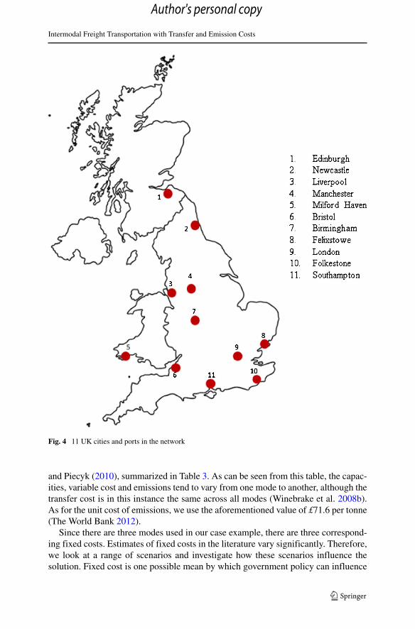
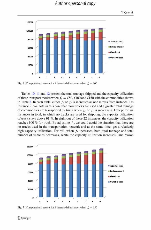
This section presents results obtained with intermodal transportation. The resultsshown in Figs. 5, 6 and 7 show the total cost, including variable cost, fixed cost, emis-sion cost and intermodal transfer cost for nine intermodal instances when ft = £50,£100 and £150, respectively. From these figures, we note that the variable cost, whichis around £75000, takes up the largest proportion of the total cost and it does notchange greatly across the 27 instances. Intermodal transfer cost takes up the leastproportion. For each ft , the total fixed cost increases when fr or fs is increasing.Hence, the total cost is also increasing. More details about the total cost and its com-ponents are presented in Table 9, which shows costs that are normalized to 1 againstbase case scenarios of ft = fr = fs , for all 27 instances.

It can be seen from Table 9 that when ft = £50, the normalized costs for the ninecorresponding instances is betwen 1.000 and 1.078. For each ft , the total fixed costis increasing as fr or fs is increasing. It is interesting that the variable cost staysrelatively stable even with the changing fixed costs, where the range of differenceis from 0.1 % to 2.3 %. For most instances, the emission cost slightly increases asfr or fs increases. The emission cost increases up to 11.6 %. We have mentionedin Section 3.1 that emission cost is measured by the product of distance, amount ofload and emission factors. We also know that emission factor for truck is the high-est, followed by ship and rail. So when fr or fs is increasing, total truck tonne-milesincrease, which results in an increase of the emission cost. Since rail and ship havelower emission factors than truck, reducing fr and fs helps reducing emission costin intermodal transportation. Transfer cost also does not change significantly acrossthe instances. The transfer cost is between 1.65 % and 3.1 % of the total cost, imply-ing that transfers are not an insignificant component of the intermodal tansportationchain, at least as far as the costs are concerned. Consolidation of loads or incen-tivizing certain low emission forms of transportation can be efficiently achieved inintermodal transportation.

Fig. 5 Computational results for 9 intermodal instances when ft = 50


Y. Qu et al.


Tables 10, 11 and 12 present the total tonnage shipped and the capacity utilizationof three transport modes when ft = £50, £100 and £150 with the commodities shownin Table 2. In each table, either fr or fs is increases as one moves from instance 1 toinstance 9. We note in this case that more trucks are used and a greater total tonnageof commodities are transported by truck when fr or fs is increasing. Except for sixinstances in total, in which no trucks are used for shipping, the capacity utilizationof truck stays above 91 %. In eight out of these 22 instances, the capacity utilizationreaches 100 % for truck. By adjusting ft , we could avoid the situation that there areno trucks used in the transportation network and at the same time, get a relativelyhigh capacity utilization. For rail, when fr increases, both total tonnage and totalnumber of vehicles decreases, while the capacity utilization increases. One reason




Table 9 Normalized costs for intermodal instances

ft fr fs Total Variable Fixed Emission Transfer

cost cost cost cost cost

£50 £50 £50 1.000 1.000 1.000 1.000 1.000

£150 1.011 1.004 1.281 0.997 0.925

£250 1.021 1.004 1.563 0.997 0.925

£150 £50 1.028 0.996 1.844 1.025 0.965

£150 1.041 1.001 2.125 1.026 0.890

£250 1.041 1.001 2.438 1.026 0.534

£250 £50 1.054 0.990 2.609 1.070 0.965

£150 1.067 0.993 2.891 1.070 0.965

£250 1.078 0.993 3.203 1.070 0.965

£100 £100 £100 1.000 1.000 1.000 1.000 1.000

£300 1.021 1.000 1.487 0.996 1.000

£500 1.039 1.023 1.744 1.003 0.559

£300 £100 1.062 0.995 2.359 1.044 1.129

£300 1.084 0.997 2.846 1.042 1.129

£500 1.106 1.013 3.128 1.057 0.963

£500 £100 1.115 0.987 3.795 1.103 0.982

£300 1.138 0.988 4.282 1.101 0.982

£500 1.160 1.005 4.564 1.116 0.816

£150 £150 £150 1.000 1.000 1.000 1.000 1.000

£450 1.030 1.009 1.436 0.998 0.840

£750 1.050 1.042 1.385 1.017 0.649

£450 £150 1.089 0.997 2.333 1.042 1.129

£450 1.122 0.997 2.846 1.042 1.129

£750 1.149 1.016 3.103 1.042 0.963

£750 £150 1.171 0.997 3.615 1.042 1.129

£450 1.204 0.997 4.128 1.042 1.129

£750 1.231 1.015 4.385 1.057 0.969

might be that it is more cost effective to travel further to consolidate onto fewervehicles when fr is high. When fr is low, using more vehicles on direct routes couldbe more attractive. The capacity utilization of rail across the 27 instances is greaterthan 77 % overall, and is greater than 84 % in 17 instances. When ft increases, thetotal tonnage transported by rail is increasing. By changing ft or fr , we might controlthe total tonnage shipped on rail. Since ships have large capacity, the average capacityutilization of ship is much less than that of truck and rail, with values around 20 %.Due to its large capacity, the number of ships used and total tonnage of commoditiestransported also do not change as much as trucks and ships.

As part of the computational experiments, we have conducted further tests wherevariable cost and capacity of rail are changed and demands are increased. In the case


Y. Qu et al.

Table 10 Comparison of the capacity utilization for 3 modes when ft = £50

Truck Rail Ship

Total Total Capacity Total Total Capacity Total Total Capacity

no. tonnage utilization(%) no. tonnage utilization(%) no. tonnage utilization(%)

1 26 741 98.28 27 8265 77.11 11 6306 19.30

2 26 741 98.28 29 9375 81.43 9 5196 19.44

3 26 741 98.28 29 9375 81.43 9 5196 19.44

4 34 939 95.23 24 7666 80.46 12 6323 17.74

5 34 939 95.23 24 8063 84.62 10 6013 20.25

6 34 939 95.23 24 8063 84.62 10 6013 20.25

7 45 1253 96.02 22 7352 84.18 12 6496 18.23

8 45 1253 96.02 22 7352 84.18 10 6410 21.58

9 45 1253 96.02 22 7352 84.18 10 6410 21.58

that the variable cost and capacity of rail are changed to £0.017 per ton-mile and3360 tonnes (Forkenbrock 2001), the results with the intermodal model suggested aunimodal transportation plan with rail being the only mode of transport used and shipvery rarely. The capacity utilization for rail is 18 % to 32 %. In the event that demandsare increased 10-fold, the results do not significantly change although the capacityutilization of rail and ship increases. In particular, rail has a much higher capacityutilization of more than 96 % and ship being more used with capacity utilization ofbetween 76 % and 88 %. Computational results for this case can be found in Table 14,15 and 16 presented in the Appendix.


Truck Rail Ship



1 0 0 N/A 29 9035 78.48 10 6257 21.07

2 0 0 N/A 31 9748 79.21 9 5544 20.74

3 0 0 N/A 33 10095 77.06 7 4463 21.47

4 6 174 100.00 25 8613 86.78 11 6939 21.24

5 6 174 100.00 25 8613 86.78 10 6766 22.78

6 7 186 91.63 25 8589 86.54 8 6647 27.98

7 17 476 96.55 24 8141 85.44 11 6641 20.33

8 17 476 96.55 24 8141 85.44 10 6468 21.78

9 18 488 93.49 24 8117 85.19 8 6349 26.72




Truck Rail Ship



1 0 0 N/A 29 9035 78.48 10 6257 21.07

2 0 0 N/A 32 9848 77.52 8 5033 21.18

3 0 0 N/A 34 10772 79.80 4 4078 34.33

4 6 174 100.00 25 8613 86.78 10 6766 22.78

5 6 174 100.00 25 8613 86.78 10 6766 22.78

6 3 87 100.00 26 8688 84.17 8 6647 27.98

7 6 174 100.00 25 8613 86.78 10 6766 22.78

8 6 174 100.00 25 8613 86.78 10 6766 22.78

9 6 174 100.00 25 8613 86.78 8 6671 28.08

5 Bi-criteria Analysis

In this paper, the multimode multicommodity network design problem has so far beentreated as a single-objective optimization problem. This was made possible by aggre-gating the two objective functions, one relevant to operational activities, and the otherto emissions, by attaching suitable cost coefficients to each. In this section, we showhow the model can be used to produce non-dominated solutions with regard to thetwo objectives, if they are treated as incommensurable. This analysis is particularlyrelevant if costs are not a prevailing factor, or are not readily available, as might be thecase for emission cost. In multi-objective optimization, a non-dominated, or Pareto-optimal, solution is where no objective can be improved without worsening at leaseone other objective (Coello and Lamont 2007). The set of Pareto-optimal solutionsform the Pareto-frontier. Decision-makers usually select a particular Pareto-optimalsolution based on their preferences on the objectives (Ghoseiri et al. 2004). One mayrefer to Palacio et al. (2013) for an application of a bicriteria optimization model to alocation problem arising in maritime logistics.

In order to find the trade-offs between minimizing total transportation cost and theamount of CO2 emissions in the multicommodity multimodal service network designproblem, we use the notation already shown in Table 1 and define the two objectivefunctions below:

(OBJ1) f1(x, y, z) =∑

k∈K

∑

(i,j)∈A

∑

m∈M

cmij x

kmij (20)

+∑

(i,j)∈A

∑

m∈M

f mij ym

ij (21)

+ 1

2w

∑

i∈N

∑

k∈K

(∑

m∈M

zkmi − hk

i

)(22)

(OBJ2) f2(x) =∑

k∈K

∑

(i,j)∈A

∑

m∈M

dmij emxkm

ij . (23)


Y. Qu et al.

In the above, f1(x, y, z) measures the total transportation cost, including variablecost, fixed cost and transfer cost, the details of which are given in Section 3.2. On theother hand, f2(x) measures the total CO2 emissions for all activities. Let S denotethe feasible set of solutions defined by the equality and inequality constraints (6)–(9),Eqs. 12 and 13 as described in Section 3.3.

A number of methods have been suggested to generate the Pareto frontier inmulti-objective programming, such as goal programming, bound objective functionformulations and genetic algorithms. In this paper, we use the ε-constraint method,which is easy to implement and effective. In this method, one of the objectives isoptimized, subject to other objective converted into a constraint by imposing appro-priate upper bounds on its value. The ε-constraint method can be implemented asfollows (Mavrotas 2009, Engau and Wiecek 2007). We first solve the followingsingle-objective optimization problem:

Minimize f2(x) (24)

subject to x ∈ S. (25)

Let an optimal solution vector of (24)–(25) be denoted by (x∗2 ). The minimized

amount of CO2 emissions is then fixed as f2(x∗2 ) = ε. Following this step, we solve

the following single-objective optimization model:

Minimize f1(x, y, z) (26)

subject to f2(x) ≤ ε (27)

x, y, z ∈ S. (28)

Let (x∗1 , y∗

1 , z∗1) denote an optimal solution to Eqs. 26–28. Furthermore, let q be thenumber of Pareto-optimal solutions that a decision-maker wishes to produce. Then,the value of ε is to be increased by ς at every iteration where:

ς = (f2(x∗1 ) − f2(x

∗2 ))/(q − 1). (29)

The method iterates by increasing the value of ε in this way (see Table 13), whereeach iteration generates another optimal solution. By repeatedly relaxing the upper

Table 13 Value of ε in the ε-constraint method

Iteration no. Value of ε

1 f ∗2

2 f ∗2 + ς

3 f ∗2 + 2ς

... ...

q − 1 f ∗2 + (q − 2)ς

q f2(x∗

1

)



Fig. 8 Pareto optimal curve of the bi-criteria model

bound on f2, and resolving f1 each time, solutions can be obtain to construct thePareto-frontier.

We now present a numerical example to illustrate the application of the ε-constraint method on the multimode multicommodity network design problem.The method is implemented in C and each sub-problem is solved to opti-mality by ILOG CPLEX Interactive Optimizer 12.4. Therefore, the solutionsgenerated are Pareto-optimal. The instances is based on the data presented inSection 4.1 with the fixed-cost scenario where ft = £50, fr = £150 andfs = £250.

Assuming q = 45, the stepsize is calculated as ς = 0.7 tonne. The resulting setof Pareto-optimal solutions are shown in Fig. 8.

Fig. 9 Normalized Pareto optimal curve of the bi-criteria model


Y. Qu et al.

To select the most preferred solution from this set of non-dominated solutions, wehave also implemented a normalized distance method, for which the two objectivesare normalized as follows:

f1(x, y, z) = f1(x, y, z) − f1(x∗

1 , y∗1 , z∗1

)

f1(x∗

2 , y∗2 , z∗2

) − f1(x∗

1 , y∗1 , z∗1

) ∈ [0, 1], (30)

f2(x) = f2(x) − f2(x∗

2

)

f2(x∗1 ) − f2

(x∗

2

) ∈ [0, 1], (31)

where f1 and f2 are the normalized value of OBJ1 and OBJ2, respectively. Assumingan ideal point (0, 0), as shown in Fig. 9, the solution that is closest can be consideredas the most preferred solution.

As seen in Fig. 9, the normalized solution that yields the minimum distance fromthe ideal point is f1 = 0.31 and f2 = 0.43. Mapping this on the original functions,the values of the corresponding solutions are OBJ1 = £85869.2 and OBJ2 = 83.1tonne.

6 Conclusions

In this paper, we have described an intermodal freight transportation model, whichextends the traditional service network design models by taking GHG emission costinto account. The model includes a nonlinear expression for transfer cost at inter-modal nodes, but one which can be linearized as shown in the paper. We have alsoshown how the problem can be formulated as a bi-objective optimization model. Thecomputational results suggest that the proposed model can provide cost-efficient andemission-efficient ways for transporting commodities. This makes it interesting forpractical applications.

One important detail to remember is that the adjusted fixed cost is used for thepurpose of sending the correct economic signals. We believe that it provides anopportunity for considerable cost reduction while adjusting fixed costs. By changingthe value of the fixed costs for the three modes of transport, the tradeoffs betweenemissions and transfer costs can be analyzed.

Acknowledgements Thanks are due to three reviewers for their valuable comments and suggestions onthe initial version of this paper. This study has been partially supported by funds provided by the Universityof Southampton which is gratefully acknowledged.

Appendix

Tables 14–16 list the capacity utilization for 3 transport modes when ft = £50, £100and £150 with 10 fold of commodities in Table 2.



Table 14 Comparison of capacity utilisation for 3 modes when ft = £50 and demand is increased 10-fold

Truck Rail Ship

Total Total Capacity Total Total Capacity Total Total Capacityno. tonnage utilization(%) no. tonnage utilization(%) No. tonnage utilization(%)

1 241 6970 99.73 207 79080 96.23 27 64370 80.272 245 7105 100.00 210 80624 96.71 25 62629 84.353 245 7105 100.00 211 80624 96.25 25 62614 84.334 289 8365 99.81 199 77805 98.48 28 63427 76.275 290 8380 99.64 200 77775 97.95 27 63355 79.016 292 8437 99.63 199 77718 98.37 27 63298 78.947 428 12370 99.66 188 73697 98.74 28 63120 75.908 430 12428 99.66 188 73630 98.65 27 63064 78.649 430 12443 99.78 188 73634 98.66 27 63092 78.68

Table 15 Comparison of capacity utilisation for 3 modes when ft = £100 and demand is increased10-fold

Truck Rail Ship

Total Total Capacity Total Total Capacity Total Total Capacityno. tonnage utilization(%) no. tonnage utilization(%) No. tonnage utilization(%)

1 0 0 N/A 225 86050 96.33 28 65670 78.972 0 0 N/A 229 87638 96.40 26 64100 83.013 0 0 N/A 229 87638 96.40 24 63042 88.444 10 279 96.21 220 85773 98.21 29 65583 76.145 11 308 96.55 220 85767 98.20 27 65211 81.326 10 279 96.21 221 85796 97.79 26 64625 83.697 22 627 98.28 217 85429 99.16 29 65671 76.258 39 1119 98.94 216 84935 99.05 27 65122 81.219 39 1119 98.94 216 84935 99.05 27 65122 81.21

Table 16 Comparison of capacity utilisation for 3 modes when ft = £150 and demand is increased10-fold

Truck Rail Ship

Total Total Capacity Total Total Capacity Total Total Capacityno. tonnage utilization(%) no. tonnage utilization(%) no. tonnage utilization(%)

1 0 0 N/A 225 86050 96.33 28 65670 78.972 0 0 N/A 229 87638 96.40 24 63042 88.443 0 0 N/A 229 87638 96.40 24 63042 88.444 5 134 92.41 220 86028 98.50 29 65865 76.475 12 337 96.84 219 85738 98.61 27 65324 81.466 5 134 92.41 220 86028 98.50 26 64530 83.577 15 424 97.47 217 85325 99.04 29 66285 76.968 16 453 97.63 217 85294 99.01 27 65919 82.209 16 453 97.63 217 85294 99.01 26 65125 84.34


Y. Qu et al.

References

Andersson E, Berg M, Nelldal B, Froidh O (2011) TOSCA: rail freight transport: techno-economic analy-sis of energy and greenhouse gas reductions. Tech. rep., KTH, Rail Vehicles, KTH, The KTH RailwayGroup, KTH, Traffic and Logistics

Arnold P, Peeters D, Thomas I (2004) Modelling a rail/road intermodal transportation system. Transp ResPart E: Logist Transp Rev 40(3):255–270

Balakrishnan A, Magnanti TL, Wong RT (1989) A dual-ascent procedure for large-scale uncapacitatednetwork design. Oper Res 37(5):716–740

Bauer J, Bektas T, Crainic TG (2009) Minimizing greenhouse gas emissions in intermodal freighttransport: an application to rail service design. J Oper Res Soc 61(3):530–542

Bektas T, Crainic TG (2007) A brief overview of intermodal transportation. In: Taylor GD (ed) Logisticsengineering handbook. CRC Press, Boca Raton

Ben-Ayed O, Blair CE, Boyce DE, LeBlanc LJ (1992) Construction of a real-world bilevel linearprogramming model of the highway network design problem. Ann Oper Res 34(1):219–254

Campbell JF, Ernst AT, Krishnamoorthy M (2002) Hub arc location problems: part I—introduction andresults. Manag Sci 51(10):1540–1555

Christiansen M, Fagerholt K, Nygreen B, Ronen D (2007) Maritime transportation. In: Barnhart C, LaporteG (eds) Transportation, handbooks in operations research and management science, vol 14. Elsevier,Amsterdam, pp 189–284

Coello CAC, Lamont GB (2007) Evolutionary algorithms for solving multi-objective problems. Springer,New Jersey

Correia I, Nickel S, Saldanha-da Gama F (2013) Multi-product capacitated single-allocation hub locationproblems: formulations and inequalities. Netw Spat Econ (in press)

Crainic TG (2000) Service network design in freight transportation. Eur J Oper Res 122(2):272–288Crainic TG, Kim K (2007) Intermodal transportation. In: Barnhart C, Laporte G (eds) Transportation,

handbooks in operations research and management science, vol 14. Elsevier, Amsterdam, pp 467–537Crainic TG, Laporte G (1997) Planning models for freight transportation. Eur J Oper Res 97(3):409–438Crainic TG, Rousseau JM (1986) Multicommodity, multimode freight transportation: a general model-

ing and algorithmic framework for the service network design problem. Transp Res B Methodol20(3):225–242

Demir E, Bektas T, Laporte G (2011) A comparative analysis of several vehicle emission models for roadfreight transportation. Transp Res D: Transp Environ 16(5):347–357

Department for Transport (2005) Truck specifications for best operational efficiency. Tech.rep., Department for Transport, London. Available at: http://www.dft.gov.uk/rmd/project.asp?intProjectID=12043. Accessed 28 Nov 2013

Department for Transport (2011) Transport statistics great britain 2011. Tech. rep., Depart-ment for Transport, London. Available at: https://www.gov.uk/government/publications/transport-statistics-great-britain-2011. Accessed 28 Nov 2013

Department for Transport (2012) Transport statistics great britain 2012. Tech. rep., Depart-ment for Transport, London. Available at: https://www.gov.uk/government/publications/transport-statistics-great-britain-2012. Accessed 28 Nov 2013

Ebery J, Krishnamoorthy M, Ernst A, Boland N (2000) The capacitated multiple allocation hub locationproblem: formulations and algorithms. Eur J Oper Res 120(3):614–631

Engau A, Wiecek MM (2007) Generating ε-efficient solutions in multiobjective programming. Eur J OperRes 177(3):1566–1579

Faulkner D (2004) Shipping safety: a matter of concern. Proc IMarEST-Part B-J Mar Des Oper2004(5):37–56

Forkenbrock DJ (2001) Comparison of external costs of rail and truck freight transportation. Transp ResA: Policy Pract 35(4):321–337

Ghoseiri K, Szidarovszky F, Asgharpour MJ (2004) A multi-objective train scheduling model and solution.Transp Res B Methodol 38(10):927–952

Holguın-Veras J, Jara-Dıaz S (2006) Preliminary insights into optimal pricing and space allocation atintermodal terminals with elastic arrivals and capacity constraint. Netw Spat Econ 6(1):25–38

Holguın-Veras J, Patil G (2008) A multicommodity integrated freight origin-estination synthesis model.Netw Spat Econ 8(2–3):309–326


http://www.dft.gov.uk/rmd/project.asp?intProjectID=12043

http://www.dft.gov.uk/rmd/project.asp?intProjectID=12043

https://www.gov.uk/government/publications/transport-statistics-great-b ritain-2011





Holmberg K, Yuan D (2000) A Lagrangian heuristic based branch-and-bound approach for the capacitatednetwork design problem. Oper Res 48(3):461–481

Janic M (2007) Modelling the full costs of an intermodal and road freight transport network. Transp ResD: Transp Environ 12(1):33–44

Janic M, Bontekoning Y (2002) Intermodal freight transport in europe: an overview and prospectiveresearch agenda. Proc Focus Group 1:1–21

Kuby M, Xu Z, Xie X (2001) Railway network design with multiple project stages and time sequencing.J Geogr Syst 3(1):25–47

Lane B (2006) Life cycle assessment of vehicle fuels and technologies. Tech., rep., Ecolane Trans-port Consultancy, Bristol. http://www.ecolane.co.uk/content/dcs/Camden LCA Report FINAL 1003 2006.pdf

Macharis C, Bontekoning YM (2004) Opportunities for or in intermodal freight transport research: areview. Eur J Oper Res 153(2):400–416

Magnanti TL, Wong RT (1984) Network design and transportation planning: models and algorithms.Transp Sci 18(1):1–55

Mavrotas G (2009) Effective implementation of the ε-constraint method in multi-objective mathematicalprogramming problems. Appl Math Comput 213(2):455–465

McKinnon A, Piecyk M (2010) Measuring and managing co2 emissions in european chemical transport.Tech. rep., Logistics Research Centre, Heriot-Watt University, Edinburgh,UK

Meng Q, Wang X (2011) Intermodal hub-and-spoke network design: incorporating multiple stakeholdersand multi-type containers. Transp Res B Methodol 45(4):724–742

Oliver J, Janssens-Maenhout G, Peters J (2012) Trends in global CO2 emissions: 2012 report. Tech,rep., PBL Netherlands Environmental Assessment Agency, Netherlands. http://edgar.jrc.ec.europa.eu/CO2REPORT2012.pdf

Palacio A, Adenso-Dıaz B, Lozano S, Furio S (2013) Bicriteria optimization model for locating maritimecontainer depots. Application to the port of valencia. Netw Spat Econ (in press)

Park D, Kim NS, Park H, Kim K (2012) Estimating trade-off among logistics cost, CO2 and time: a casestudy of container transportation systems in Korea. Int J Urban Sci 16(1):85–98

Steenbrink PA (1974) Transport network optimization in the Dutch integral transportation study. TranspRes 8(1):11–27

Szeto W, Jiang Y, Wang D, Sumalee A (2013) A sustainable road network design problem with land usetransportation interaction over time. Netw Spat Econ (in press)

The World Bank (2012) Carbon finance unit. Available at: http://www.worldbank.org/en/topic/climatefinance. Accessed 28 Nov 2013

Treitl S, Nolz P, Jammernegg W (2012) Incorporating environmental aspects in an inventory routingproblem. A case study from the petrochemical industry. Flex Serv Manuf J (in press)

Vidovic M, Zecevic S, Kilibarda M, Vlajic J, Bjelic N, Tadic S (2011) The p-hub model with hub-catchment areas, existing hubs, and simulation: a case study of serbian intermodal terminals. NetwSpat Econ 11(2):295–314

Winebrake JJ, Corbett JJ, Falzarano A, Hawker JS, Korfmacher K, Ketha S, Zilora S (2008a) Assess-ing energy, environmental, and economic tradeoffs in intermodal freight transportation. J Air WasteManag Assoc 58(8):1004–1013

Winebrake JJ, Corbett JJ, Hawker JS, Korfmacher K (2008b) Intermodal freight transport in the greatlakes: development and application of a great lakes geographic intermodal freight transport model.Tech. rep., Rochester, US

Yamada T, Russ BF, Castro J, Taniguchi E (2009) Designing multimodal freight transport networks: aheuristic approach and applications. Transp Sci 43(2):129–143

Zografos KG, Regan AC (2004) Current challenges for intermodal freight transport and logistics in europeand the united states. Transp Res Rec: J Transp Res Board 1873:70–78


http://www.ecolane.co.uk/content/dcs/Camden_LCA_Report_FINAL_10_03_2006.pdf

http://www.ecolane.co.uk/content/dcs/Camden_LCA_Report_FINAL_10_03_2006.pdf

http://edgar.jrc.ec.europa.eu/CO2REPORT2012.pdf

http://edgar.jrc.ec.europa.eu/CO2REPORT2012.pdf

http://www.worldbank.org/en/topic/climatefinance

http://www.worldbank.org/en/topic/climatefinance

Sustainability SI-Multimode Multicommodity Network Intermodal Transportation With Emission Costs

Documents

Transcript of Sustainability SI-Multimode Multicommodity Network Intermodal Transportation With Emission Costs