SUSTAINABILITY OF THE US CURRENT ACCOUNT …ageconsearch.umn.edu/bitstream/37640/2/ansari.pdf · by...

249SUSTAINABILITY OF THE US CURRENT ACCOUNT DEFICIT

Journal of Applied Economics, Vol. VII, No. 2 (Nov 2004), 249-269

SUSTAINABILITY OF THE US CURRENTACCOUNT DEFICIT: AN ECONOMETRICANALYSIS OF THE IMPACT OF CAPITAL

INFLOW ON DOMESTIC ECONOMY

MOHAMMED I. ANSARI*

Albany State University

Submitted September 2003; accepted February 2004

The purpose of this paper is to estimate, by using the recent econometric techniques of unitroot testing and Johansen-Juselius cointegration technique (1990), the impact of foreigncapital inflow on the volume and efficiency of domestic investment in the United Statesduring the period, 1973-1999. A battery of diagnostic tests is employed to check the validityand robustness of the estimated results. Evidence suggests that capital inflows have had asignificant positive effect on the volume of US investment, but the effect on the efficiencyof investment has been minimal. These findings imply that, while achieving current accountbalance is important, it is equally important to sustain and augment the beneficial impactof capital inflow by creating a more conducive investment climate. Given our limitedability to influence current account balance, this seems to be a more pragmatic policyoption for dealing with the US current account imbalance.

JEL classification codes: F21, F41, O51

Key words: current account, capital inflow

I. Introduction

The persistently growing US current account deficit has attracted a good

* The author is grateful to the Faculty Research Committee, Albany State University, forproviding funding for this project under its Title III Programs for Fall 2002. A preliminarydraft of this paper was presented in the 29th Annual Conference of the Academy ofEconomics and Finance, and a revised version was presented in the 5th Annual InternationalBusiness and Economics Conference. The author likes to express his gratitude to the tworeferees and the editor of this journal for making valuable comments and suggestions. Theusual disclaimer applies.

250 JOURNAL OF APPLIED ECONOMICS

deal of attention from researchers and policy makers alike. Many view the

situation as unsustainable and even downright calamitous.1 There are many

reasons why a rapidly rising current account deficit is looked at with such a

disdain. First, current account deficit complicates domestic demand

management policy. The concomitant rise in capital account surplus can feed

into booming equity market creating wealth effect. Further, pursuing a tight

monetary policy to dampen demand pressures, can create supply bottlenecks

by discouraging investment and exacerbate inflationary pressures. Thus,

current account imbalance can potentially confound and complicate

macroeconomic policy, making it harder to maintain price stability and achieve

long term economic growth. Second, many studies have shown that a nation’s

unfavorable balance of payment has the potential to constrain its long term

economic growth.2 Third, there is always a danger of a sudden and a large

scale withdrawal of foreign capital, creating, what Peter Drucker calls, the

looming transfer crisis (1988).

But a more realistic approach to the sustainability issue must take into

account the impact of foreign capital inflow on the national economy. Just as

a large and persistently growing current account deficit can have a detrimental

effect, a large and persistently growing capital account surplus, which mirrors

the current account balance, can have a beneficial effect on the economy. The

1 Lester Thurow says, “...to run a trade deficit, a country must borrow from the rest of theworld...as debts grow, interest payments grow...as time passes, the rate of debt accumulationspeeds up...compound interest eventually insures that the remained annual borrowingsbecome so large that the rest of the world will be unable to lend the necessary sums... whenthat happens, dramatic changes occur,” (1992, pp. 236-237). Paul Krugman goes one stepfurther and maintains that “the (U.S.) trade deficit remains huge; meanwhile foreignershave bought up a large quantities of U.S. assets at bargain prices, thanks to a weakerdollar...a financial squeeze to the U.S. due to a cutoff of foreign capital is not only a livepossibility, it is arguably already in process,” (1995, p. 36).

2 “In the long run, no country can grow faster than at the rate consistent with balance ofpayments equilibrium on current account, and if the real terms of trade do not changemuch, this rate is determined by the rate of growth of export volume divided by the incomeelasticity of demand for imports. Attempts to grow faster than this rate mean that exportscannot pay for imports, and the economy comes against a balance of payments constrainton demand, which affects the industrial sector’s ability to grow as fast as labor productivity,”(Thirlwall, 1982, p. 33).


balance sheets of many highly successful corporations show an extremely

high debt to equity ratio. But, so long as these corporations have a good cash

flow and earn a high rate of return on their investment, heavy debt burden

does not mire their future growth potential. To a large extent, the analogy

may apply to a country’s balance sheet. It is conceivable that the United States

has done well in recent years because of and not despite rising foreign debt.

Preliminary calculations show that the US economy has grown at an annual

average rate in excess of 3 percent over 1970 and 1999, considered to be the

country’s long term secular growth rate. This is also the period which marked

a rising trend in the current account deficit. It is noteworthy that the rate of

growth excluding 1991, the year of the previous recession, has been about

3.6 percent. During the same period, the US has experienced the fastest rate

of deterioration in the country’s current account balance. Are these just

coincidences and statistical artifacts or there is more to them than meets the

eye? The purpose of this study is to find some answers. More specifically, we

estimate econometric models to determine the impact of foreign capital inflow

on the volume and the efficiency of domestic investment. To avoid spurious

results, we employ recently developed and widely used time series

methodologies for establishing the statistical properties of the data set. A

battery of diagnostic tests is employed to verify the validity and robustness of

these results. These findings suggest that, while reducing the current account

deficit is important, it is equally important to augment the beneficial impact

of capital inflow. Given the limited ability to influence current account balance,

this seems to be a more pragmatic policy option for dealing with the US

current account imbalance.

The rest of the paper is organized as follows. Section II presents a synopsis

of the US current and capital account balance. Section III explains the literature,

the model, and the methodology. Empirical results are analyzed in section IV.

Section V consists of a few concluding remarks.

II. The US Current and Capital Account Balance: A Synopsis

The United States has seen significant structural changes in its external

economy over the past 50 years. It enjoyed the status of a creditor nation


during the 1950’s, 1960’s and a balanced status during much of the 1970’s.3

But it has gradually earned the status of the largest debtor nation in recent

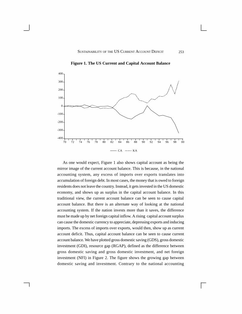
years. To obtain a visual impression of the magnitude of these changes, we

have shown the time series behavior of current account (CA) and capital

account (KA) balance in Figure 1. The figure clearly shows the transition as

the country moved from the position of equilibrium during much of the 1970’s

to a position of deficit, especially following a large appreciation of the dollar

in the first half of the 1980s. This trend is seen to have reversed itself in the

second half of the 1980s following an equally large depreciation of the dollar.

The 1991 recession further helped improve the balance. However, the declining

trend resumed and even accelerated thereafter. The longest peace time

expansion, coupled with the strengthening dollar, has caused the current

account deficit to reach an all time high in the 1990’s.4

It has often been pointed out that the dollar value of the deficit presents an

exaggerated picture as it does not account for the size of the economy. To

redress this, we computed the ratio of current account balance to total GDP.

This ratio has ranged from a high of about 1 percent in 1975 to a low of about

-3.6 percent in 1999, with an average of an about -1 percent over the sample

period. The years of external deficit has caused our foreign indebtedness to

swell. What is the critical level of foreign indebtedness for a country like the

USA? There is no clear cut answer to this question. Evidence shows that

many nations in the past, including Canada and Australia, have carried several

times higher debt burden than the US. At the risk of simplification, one might

say that external debt is limited only by total foreign wealth and the foreigner’s

ability and willingness to continue lending.

3 The large current account surplus of the 1950’s and 1960’s was made possible mainlybecause the country enjoyed a unique and enviable trade competitiveness position whichled to an unprecedented export boom. Faced with a growing challenge by major economieslike Japan and Germany, coupled with unfavorable exchange rate changes and the impactof large energy imports, the country began to see a deterioration in its external balance inthe 1970’s.

4 The gradual improvement in the US service account balance over the sample periodprovides one bright spot in this otherwise dismal scenario. See Ansari and Ojemakinde(2003) for a detailed discussion of the asymmetric behavior of the merchandise and serviceaccount balance.


Figure 1. The US Current and Capital Account Balance

-400

-300

-200

-100

0

100

200

300

400

70 72 74 76 78 80 82 84 86 88 90 92 94 96 98 00

CA KA

As one would expect, Figure 1 also shows capital account as being the

mirror image of the current account balance. This is because, in the national

accounting system, any excess of imports over exports translates into

accumulation of foreign debt. In most cases, the money that is owed to foreign

residents does not leave the country. Instead, it gets invested in the US domestic

economy, and shows up as surplus in the capital account balance. In this

traditional view, the current account balance can be seen to cause capital

account balance. But there is an alternate way of looking at the national

accounting system. If the nation invests more than it saves, the difference

must be made up by net foreign capital inflow. A rising capital account surplus

can cause the domestic currency to appreciate, depressing exports and inducing

imports. The excess of imports over exports, would then, show up as current

account deficit. Thus, capital account balance can be seen to cause current

account balance. We have plotted gross domestic saving (GDS), gross domestic

investment (GDI), resource gap (RGAP), defined as the difference between

gross domestic saving and gross domestic investment, and net foreign

investment (NFI) in Figure 2. The figure shows the growing gap between

domestic saving and investment. Contrary to the national accounting


framework in which resource gap and net foreign capital inflow should be

identical, Figure 2 shows some discrepancy. Statistical discrepancy in the

balance of payment account explains the observed difference between the

two. Here, resource gap (RGAP) reflects the amount of net foreign capital

inflow (NFI) that the country needs to restore equilibrium in the economy.

This discussion makes it clear that there is no a priori basis for assuming the

direction of causation one way or the other. However, since causality between

the two accounts is not the main focus of this paper, we abstain from any

further discussion of the subject.5

5 Results from a preliminary causality test for the US, not reported here, indicate thatcapital account balance has caused current account balance in the Granger sense.

Figure 2. Saving, Investment, and Resource Gap

-400

0

400

800

1200

1600

2000

1970 1972 1974 1976 1978 1980 1982 1984 1986 1988 1990 1992 1994 1996 1998

GDSGDI

RGAPNFI

III. Literature, Model, and Methodology

Most of the literature on the subject, both theoretical and empirical, has

evolved in the context of the developing countries. In the 1950’s and 1960’s

foreign capital, by and large, was seen to augment growth in the developing


countries both through its resource augmentation effect, and with certain

assumptions regarding capacity utilization, gestation period, and composition

of output, through favorable effect on the efficiency of domestic investment.

The resource augmentation effect is believed to take two forms. There is a

direct effect, which stems from the fact that foreign capital provides additional

investible funds, adding directly to total volume of domestic investment. But

foreign capital can also affect volume of domestic investment in another and

indirect way. To the extent foreign capital augments national income, it can

help generate additional domestic saving, which in turn, can cause domestic

investment to rise. The impact of foreign capital on the efficiency of domestic

investment can take many forms and can flow from many channels. For

instance, it can raise incremental output-capital ratio (IOCR), total factor

productivity (TFP), and labor productivity (LP). It has been argued that, by

helping reduce price distortions, foreign capital can facilitate pricing of inputs

and outputs to reflect relative scarcities, and thereby, enhance efficiency.

By the 1970’s the once one-sided view of foreign capital began to change.

It was, for instance, recognized that much of the benefits will be lost if foreign

capital is used to finance consumption. There is always a possibility that foreign

capital may cause governments to lax their tax efforts, increase consumption,

and induce the country to import more. It is also argued that foreign capital

may pre-empt private investment opportunities, crowding-out domestic

investment. Further, accompanied by wrong technology and inefficient

management, foreign capital can actually have adverse effect on the efficiency

of investment. It is easy to see that, given many and sometimes conflicting

possibilities, the impact of foreign capital on domestic economy becomes an

empirical issue.

In the past investigators have adopted several routes while trying to assess

the impact of foreign capital on domestic economy. Many researchers have

focused on the relationship between foreign capital and domestic saving, i.e.,

the resource effect. Others have tried to study the relationship between foreign

capital and output-capital ratio, i.e., the efficiency effect. Yet others have

focused on the relationship between foreign capital and economic growth

through capital formation. These studies seem to have produced mixed results.

Rahman (1968), Griffin and Enos (1970), and Areskoug (1973) are some of

the earlier studies falling into the first category. With some minor differences,


these studies found that foreign capital substituted for domestic saving only

partly, implying that foreign capital had a positive effect on domestic saving.

Weisskopf (1972), using both cross-section and time series data from less

developed countries, also reached a similar conclusion. However, Papanek

(1972), using pooled data in a disaggregated study, found that foreign capital

had a negative effect on domestic saving. Similarly, Fry (1984) using time-

series data from 1960 to 1980 for Bangladesh, Korea, Nepal and Thailand,

found that foreign capital had a net negative effect on domestic saving only

in Bangladesh. In another study, Gupta and Islam (1983), using cross-section

data for eighteen Asian countries, found a positive effect of foreign capital

on domestic saving with no substitution effect. Stoneman (1975), Papanek

(1973), Dowling and Hiemenz (1983), and Gupta and Islam (1985), using

pooled cross-section time series data, estimated a neoclassical production

function and found that foreign capital had a positive effect on capital formation

and hence on economic growth in many developing countries. Voivodas (1974)

and Go (1985) also found a positive effect of foreign capital on investment

and economic growth when they estimated an investment function using

foreign capital as an independent variable. Voivodas (1973), on the other

hand, using incremental output-capital ratio as a proxy for efficiency of

investment and pooled data from twenty developing countries, found that

foreign capital had a negative effect on the efficiency of investment.

Despite their contribution to the existing knowledge on the subject, most

of these studies suffered from two serious problems. First, invariably, all these

studies depended on a single equation model. It is well known fact that single

equation specifications suffer from a simultaneity problem. And second, none

of these studies paid sufficient attention to the issue of stationarity in the data

set. It is commonly agreed fact that most of the macroeconomic time series

data are non-stationary, which can render the estimated results invalid and

unreliable.

This study differs from the earlier studies in that we explicitly deal with

the issue of stationary. All data series are pre-tested to establish their time

series characteristics. Also, consistent with the objective of this paper, we

estimate vector autoregressive models. The resource effect of foreign capital,

for instance, is studied by estimating a three-variable VAR model with

domestic saving, domestic income, and foreign capital. Of course, the


specification of the VAR model depends on the actual time series

characteristics of the data set. If, for instance, the variables are integrated but

not cointegrated, a VAR in difference may provide an appropriate specification.

But if the variables are integrated and also cointegrated, then a vector error-

correction model (VECM) provides a more efficient specification. We estimate

a bivariate model with incremental output-capital ratio and foreign capital to

test for the efficiency effect of foreign capital.

The VAR methodology is so commonly used that only a brief discussion

is warranted here. A vector error-correction model retains all other benefits

of an unrestricted VAR. Like VAR, it is also a generalized reduced form

which helps detect the statistical relationship among the variables in the system.

It allows all variables to interact with itself and with each other, without having

to impose a theoretical structure on the estimates. Moreover, it provides a

convenient method of analyzing the impact of a given variable on itself and

on all others by using variance decompositions (VDCs) and impulse response

functions (IRFs). In estimating VECM, the residuals from the cointegrating

equations are included as error-correction terms. If the coefficients of the

error-correction terms are found to be statistically significant, it implies that

any deviation from long run equilibrium is corrected by short-run adjustment

process. Thus, the error-correction terms provide additional channels for

capturing causality.

It is widely known that many time series data suffer from non-stationarity

problem which may undermine the validity of the estimated parameters. For

these and other reasons, it is important to conduct a unit root test on the data

set. Since the idea is not new and the techniques are widely used, only a brief

description is presented here. A series is considered stationary if its mean,

variance and covariances are time-independent. The two most frequently used

unit root tests are the Dickey-Fuller (DF) and the Augmented Dickey-Fuller

(ADF) tests. The ADF test uses an equation of the following form:

p

dxt = α

0 + α

1 x

t-1 + Σ α

2i dx

t-i + e

t (1)

i = 1

where d is the first difference operator and et is a zero mean white noise error-

term. The null hypothesis that xt contains a unit root (is non-stationary) amounts


to testing H0: α

1 = 0. The null hypothesis is rejected if α

1 takes a negative value

and is significantly different from zero, in which case the series is consideredstationary. The lag structure is chosen such that the error-term, e

t becomes

white noise. The test statistic has a special distribution (Fuller, 1976). The DFtest is used by omitting the summation term in equation (1). In case a given

series turns out to be non-stationary (contains a unit root), these tests arerepeated using the series in its first difference. If the null hypothesis of unit

root is rejected, then the series is said to be integrated of order one, or I(1).Next, we employ the Johansen-Juselius cointegration method to test for the

existence of a long run equilibrium economic relationships among the variablesin the model, namely, sr, yr, and kr in the United States, during the period

1973Q1-1999Q4. In a bivariate case, each of the two series, xt and y

t can

individually be non-stationary, I(1), but a linear combination of the two, say,

zt = x

t - σ y

t, can either be non-stationary, I(1) or stationary, I(0). In general, two

variables are said to be cointegrated if both are integrated of order k, but a linear

combination of the two is integrated of order less than k. As a general rule, forcointegration all variables should have the same order of integration. The

rejection of the null hypothesis of no cointegration establishes the existence ofa long-run equilibrium relationship between variables in the system. This

methodology is essentially the one proposed by Johansen (1988) and Johansenand Juselius (1990), and is the most commonly used for this kind of problems.6

IV. Empirical Results

All estimations have been carried out using quarterly data covering the

period 1973Q1 to 1999Q4. The sample period is justified by data availability.All data series used in estimating the resource effect (sr, yr, kr) are in real terms.

Real domestic saving (sr) has been obtained by deflating nominal grossdomestic saving, taken from Bureau of Economic Analysis, Department of

Commerce, by the GDP deflator, 1995 = 100, from International FinancialStatistics. The real GDP data (yr) is in 1996 prices and was obtained from IFS,

CD-ROM. Similarly, real capital flow data (kr) was obtained by deflatingnominal capital flow data from IFS, CD-ROM, using the GDP deflator

6 The use of two-step Engle and Granger methodology for testing cointegration has beencriticized on several grounds. For a detailed discussion of this issue, see Murthy and Phillips(1996).


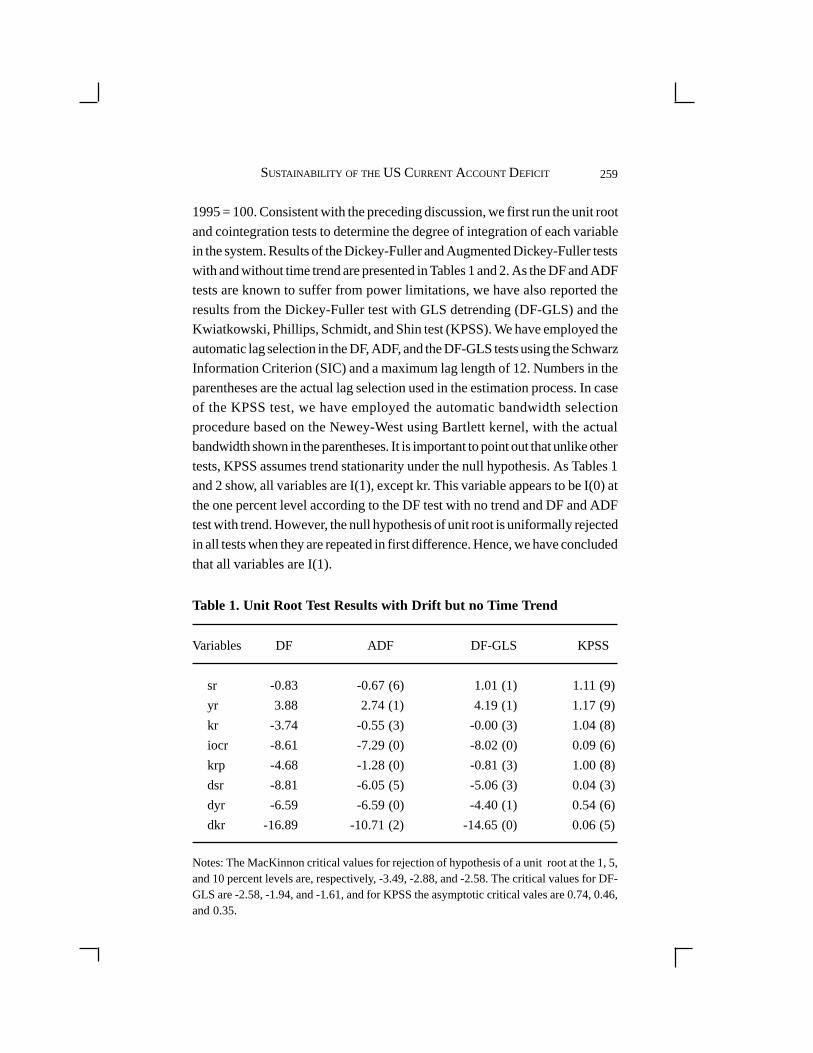
1995 = 100. Consistent with the preceding discussion, we first run the unit root

and cointegration tests to determine the degree of integration of each variablein the system. Results of the Dickey-Fuller and Augmented Dickey-Fuller tests

with and without time trend are presented in Tables 1 and 2. As the DF and ADFtests are known to suffer from power limitations, we have also reported the

results from the Dickey-Fuller test with GLS detrending (DF-GLS) and theKwiatkowski, Phillips, Schmidt, and Shin test (KPSS). We have employed the

automatic lag selection in the DF, ADF, and the DF-GLS tests using the SchwarzInformation Criterion (SIC) and a maximum lag length of 12. Numbers in the

parentheses are the actual lag selection used in the estimation process. In caseof the KPSS test, we have employed the automatic bandwidth selection

procedure based on the Newey-West using Bartlett kernel, with the actualbandwidth shown in the parentheses. It is important to point out that unlike other

tests, KPSS assumes trend stationarity under the null hypothesis. As Tables 1and 2 show, all variables are I(1), except kr. This variable appears to be I(0) at

the one percent level according to the DF test with no trend and DF and ADFtest with trend. However, the null hypothesis of unit root is uniformally rejected

in all tests when they are repeated in first difference. Hence, we have concluded

that all variables are I(1).

Table 1. Unit Root Test Results with Drift but no Time Trend

Variables DF ADF DF-GLS KPSS

sr -0.83 -0.67 (6) 1.01 (1) 1.11 (9)

yr 3.88 2.74 (1) 4.19 (1) 1.17 (9)

kr -3.74 -0.55 (3) -0.00 (3) 1.04 (8)

iocr -8.61 -7.29 (0) -8.02 (0) 0.09 (6)

krp -4.68 -1.28 (0) -0.81 (3) 1.00 (8)

dsr -8.81 -6.05 (5) -5.06 (3) 0.04 (3)

dyr -6.59 -6.59 (0) -4.40 (1) 0.54 (6)

dkr -16.89 -10.71 (2) -14.65 (0) 0.06 (5)

Notes: The MacKinnon critical values for rejection of hypothesis of a unit root at the 1, 5,and 10 percent levels are, respectively, -3.49, -2.88, and -2.58. The critical values for DF-GLS are -2.58, -1.94, and -1.61, and for KPSS the asymptotic critical vales are 0.74, 0.46,and 0.35.


Table 2. Unit Root Test Results with Drift and a Time Trend

Variables DF ADF

sr -2.30 -2.74 (3)

yr 0.57 -0.14 (1)

kr -7.01 -4.56 (0)

iocr -8.61 -7.26 (0)

krp -7.81 -7.81 (0)

dsr -8.77 -6.02 (5)

dyr -7.34 -6.59 (0)

dkr -16.82 -10.71 (2)

Notes: The MacKinnon critical values for rejection of hypothesis of a unit root for testwith drift and a time trend, at the 1, 5, and 10 percent levels are, respectively, -4.04, -3.45,and -3.15.

Next, we have used the Johansen and Juselius method to test for the

existence of a long run equilibrium relationships among the three variables

used in the model testing the resource effect, namely, sr, yr, and kr. The

estimation was carried out using one-period lag based on the Schwarz (SIC)

and Akaike (AIC) information criteria, with no deterministic trend and

restricted intercept. To enhance the robustness of the results, we have employed

both the trace and the maximum eigenvalue tests statistics. The critical values

are taken from Osterwald-Lenum (1992). The results of this test are shown in

Table 3. Looking at the table, we find that both the trace and eigenvalue

statistics exceed the critical values up to one cointegrating vector, implying

rejection of the null hypothesis and allowing us to conclude the existence of

two cointegrating vectors. This establishes the existence of a long run

equilibrium relationship among the three variables. It means that short term

deviations from this long run equilibrium will have an impact on the changes

in the dependent variable in a way which will bring the relationship back to

equilibrium once again. As Engle and Granger (1987) have shown, since

variables in the model are cointegrated, an error-correction model provides a

more efficient choice of methodology for testing the resource effect.


Table 3. Johansen and Juselius Cointegration Tests

Trace test Maximum eigenvalue test

Null Trace statistic Null Max. eigenvalue

r = 0 65.06 r = 0 36.65

(41.07) (26.81)

r ≤ 1 28.40 r = 1 20.97

(24.60) (20.20)

r ≤ 2 7.43 r = 2 7.43

(12.97) (12.97)

Note: Numbers in the parentheses are the one percent critical values.

A. Resource Effect of Foreign Capital

Engle and Granger (1987) have shown that if variables are integrated and

also cointegrated, they have a valid error-correction representation. In

estimating a vector error-correction model, cointegration approach helps

capture the dynamics of the short run relationships. Accordingly, we have

estimated a three-variable (sr, yr, kr) vector error-correction model using two

cointegrating vectors and an optimal lag structure of five periods, as determined

by the Akaike information criterion (AIC) and Schwarz information criterion

(SIC). The results of this estimation are presented in Table 4. As is the case

with unrestricted VAR, individual coefficients from the VECM model are

also hard to interpret. We have, therefore, analyzed the dynamic properties of

the model with the help of the impulse response functions and the variance

decompositions analysis. Consistent with the main thrust of the paper and to

capture the maximum impact of krt, on sr

t, we have placed kr

t first followed

by yrt and sr

t the last. Since the results from VAR models are known to be

sensitive to the ordering of the variables, we have tried different ordering, but

this did not alter the results in any significant ways. The impulse response

functions, not shown here to conserve space, indicate that a one-time one

standard deviation shock applied to yrt produced a positive impact on sr

t in

both short and long run. More importantly, a one-time one standard deviation


shock applied to krt produced a positive impact on sr

t, with the impact

magnifying over time. They also show a significant positive impact of krt on

yrt. This may be viewed as an evidence in support of our earlier contention

that foreign capital may augment domestic saving by augmenting domestic

income. It is important to point out that this indirect effect of krt on sr

t via yr

t

is not captured in a single equation model.

Table 4. Vector Error-correction Results with dsrt as the DependentVariable

Independent variables

Lag dyrt

dkrt

dsrt

1 0.017 -0.09 0.39

(0.28) (-0.72) (3.70)*

2 0.06 -0.11 -0.20

(0.86) (-0.81) (-1.98)***

3 0.00 -0.01 0.43

(0.00) (-0.07) (4.64)*

4 0.02 -0.36 -0.31

(0.32) (-2.95)* (-3.08)*

5 -0.05 0.11 0.01

(-0.80) (1.00) (0.15)

EC terms: v1t-1

= 0.006 v2t-1

= 0.23 AIC = 30.5 SC = 32.0 R2 = 0.45

(1.96)*** (2.26)**

Notes: Numbers in the parentheses are the t-values. * significant at the one percent level. **

significant at the five percent level. *** significant at the ten percent level.

Impulse response functions show the signs of the dynamic multipliers,

but they do not give any indication of their size and magnitude. For this, we

must rely on variance decompositions, as presented in Table 5. The table

shows that foreign capital inflow have had a delayed, but sharply rising impact

on srt, the proportion of variance explained by kr

t reaching over 28 percent


Table 5. Decomposition of Variance Error from VECM

Dependent Explained by innovation in:

variable yrt

krt

srt

srt

1 25 6.12 0.30 93.56

2 42 7.12 0.38 92.50

3 51 9.84 0.98 89.18

4 63 12.55 2.17 85.28

8 84 19.68 11.74 68.58

12 100 21.88 28.15 49.97

16 120 23.88 40.34 35.78

20 140 24.90 49.08 26.02

yrt

1 45 98.88 1.12 0.00

2 71 99.51 0.48 0.01

3 96 97.92 1.50 0.58

4 118 95.96 2.68 1.36

8 206 79.78 13.36 6.86

12 293 69.67 23.90 6.43

16 388 62.58 33.04 4.38

20 495 55.92 41.22 2.86

krt

1 30 0.00 100.00 0.00

2 32 0.42 99.58 0.00

3 33 2.40 97.60 0.00

4 34 4.78 95.14 0.08

8 40 7.66 90.78 1.56

12 45 9.76 88.80 1.44

16 50 11.53 87.21 1.26

20 55 12.80 85.98 1.22

Ordering: krt, yr

t, sr

t

Period S.E.


within three years and over 49 percent within five years. The impact of yrt on

srt, on the other hand, has been relatively modest in the beginning, reaching a

maximum of about 25 percent. Thus, both the impulse response functions

and the variance decompositions show a large and positive impact of krt on

srt. The table also shows, a large and a growing impact of kr

t on yr

t, the

proportion of explained variance error approaching over 40 percent. This is

in line with our earlier statement about the indirect effect of foreign capital

on domestic saving.

The coefficients of the two error-correction terms deserve a special mention.

As seen in Table 4, both coefficients of error-correction terms (EC) are

statistically significant. It means that the two independent variables (yrt, kr

t)

are related with the dependent variable (srt) in the Granger sense through the

error-correction terms. Whenever the actual value of srt deviates from its long

run equilibrium value, a change in yrt and kr

t helps bring it back to the long

term equilibrium value, other things being equal. It is in this sense that error-

correction terms provide additional channels of causation. It is worth noting

that both coefficients are positive. In a two-variable case, the sign of the EC

term is negative for bringing the system back to its long run equilibrium

whenever there is a short term deviation from the long run path. However in

a three or more variable model, the signs of the EC terms are indeterminate

and the feed back effects among the variables ensure the stability of the model

(Enders, 1995, p. 380, Rousseau and Wachtel, 1998). To sum, the results

from vector error-correction model are strong and consistent, implying a fair

degree of robustness.7

B. Efficiency Effect of Foreign Capital

As pointed out earlier in the paper, with certain assumptions, foreign capital

inflow is expected to generate significant efficiency effect on domestic

investment. This efficiency effect can take many forms, a change in incremental

output-capital ratio( IOCR) is one of them. For the purpose of this study, we

7 A pairwise Granger causality test based on the results from the vector-error-correctionmodel, not reported here to conserve space, also indicated a strong uni-directional causationfrom kr

t to sr

t, further enforcing the robustness of these results.


have defined this variable as the ratio of change in output (dy/y) to investment

rate (I/y), where y is real income, dy is change in real income, and I is

investment. We have used gross fixed capital formation, taken from

International Financial Statistics (IFS), CD-ROM and deflated by the implicit

price index, 1995 = 100, as the proxy for real investment. The following

equation has been estimated to test the efficiency effect.

iocrt = β

0 + β

1 krp

t + e

t (2)

where krpt is the ratio of total foreign capital inflow to total GDP, both in real

terms, and iocrt is incremental output-capital ratio, as defined above. As shown

in Tables 1 and 2, both variables are stationary I(0) according to various unit

root tests applied. Accordingly, we estimated equation (2) employing standard

regression techniques, without having to worry about the results being

spurious. It produced the following results,

iocrt = 0.05 + 0.11 krp

t, R2 = 0.08, DW = 2.04,

(0.85) (0.92)

with the numbers in the parentheses being the t-values. Judging by the size of

the adjusted R2, the model did not perform well. Also, the coefficient of krpt,

although has the expected sign, it is not found to be statistically significant.

From this one can deduce that the impact of foreign capital on the efficiency

of investment is not significant. To check the stability of the coefficient, we

employed the recursive least squares method. The plot of the coefficient is

produced in Figure 3. Looking at the picture, it appears that the coefficient

has experienced some improvement, implying that the impact of foreign capital

on efficiency of investment has been increasing over time. This equation was

also estimated with Almon distributed lag method to capture both the short

and the long term impact.

The results not produced here to conserve space, showed that ten out of

twelve short run coefficients had a positive sign, but none were statistically

significant. Similarly, the long run coefficient had the expected sign, but was

not found to be statistically significant. There are several plausible explanations

for somewhat muted efficiency effect of foreign capital. First, the impact of


foreign capital on the efficiency of investment is contingent upon certain

assumptions about capacity utilization rate, gestation period, and composition

of output. A violation of any or all of these assumptions can compromise the

expected results. Before drawing any definitive conclusions, therefore, one

has to do a thorough study of whether, in fact, some or all of these assumptions

were violated. Second, a non-violation of these assumptions does not guarantee

a positive efficiency effect of foreign capital inflow. Much will also depend

on the quality of management and the kind of technology which accompanies

foreign capital. The US being a highly developed country, it is quite likely

that foreign capital inflow did not bring any noticeable improvement in either

the quality of management or in the level and sophistication of technology.

V. Concluding Remarks

In this paper we set out to investigate the sustainability of the US current

account deficit by assessing the impact of capital inflow on the US economy.

The results seem to suggest that capital inflow have had a positive effect on

the economy both directly by increasing the availability of investible resources

Figure 3. Recursive Behavior of the Coefficient of Foreign Capital

-60

-40

-20

0

20

40

60

80

1976 1978 1980 1982 1984 1986 1988 1990 1992 1994 1996 1998

Recursive C(2) Estimates ± 2 S.E.


and indirectly by augmenting domestic income and saving. A battery of

diagnostic tests was employed to check the validity and robustness of these

results. The test on the efficiency effect of foreign capital, though produced

positive coefficient, was not found to be statistically significant. There are

several plausible explanations, as explained previously. The main implication

is that, while achieving current account balance is important, it is equally

important to sustain and augment the beneficial impact of capital inflow by

creating conducive investment climate. Given our limited ability to influence

current account balance, this seems to be a more pragmatic policy option for

dealing with the US current account imbalance.

References

Ansari, Mohammed I., and Abiodun Ojemakinde (2003), “Explaining

Asymmetry in the US Merchandise and Service Account Balance: Does

the Service Sector Hold the Key to the US Current Account Woes?,” The

International Trade Journal 17: 51-80.

Areskoug, Kaj (1973), “Foreign Capital Utilization and Economic Policies

in Developing Countries,” Review of Economics and Statistics 55: 182-

189.

Dickey, David A., and Wayne A. Fuller (1979), “Distribution of the Estimators

for Autoregressive Time Series with a Unit Root,” Journal of American

Statistical Association 74: 427-431.

Drucker, Peter (1988), “The Looming Transfer Crisis,” Institutional Investor

6/88: 29.

Enders, Walter (1995), Applied Econometric Time Series, New York, John

Wiley and Sons.

Engle, Robert F., and Clive W.J. Granger (1987), “Co-integration and Error

Correction: Representation, Estimation, and Testing,” Econometrica 55:

251-276.

Fry, Maxwell J. (1984), “Domestic Resource Mobilization through Financial

Development: Appendixes,” ADB, Economics Office, February.

Fuller, Wayne A. (1976), Introduction to Statistical Time Series, New York,

John Wiley and Sons.

Go, Evelyn (1985), “The Impact of Foreign Capital Inflow on Investment


and Economic Growth in Developing Asia,” ADB, Economics Office,

Report Series, no. 33.

Graham, Edward M., and Paul R. Krugman (1991), “Foreign Direct Investment

in the United States,” Institute for International Economics.

Gray, Peter H. (1982), “Macroeconomic Theories of Foreign Direct

Investment: An Assessment,” in A. M. Rugman, eds., New Theories of

the Multinational Enterprise, London, Groom Elm.

Griffin, Keith B., and John L. Enos (1970), “Foreign Assistance: Objectives

and Consequences,” Economic Development and Cultural Change 18:

313-327.

Gupta, Kanhaya L. and M. Anisul Islam (1983), Foreign Capital, Savings

and Growth, Boston, Reidel.

Higgins, Matthew, and Thomas Klitgaard (1998), “Viewing the Current

Account Deficit as Capital Inflow,” Current Issues in Economics and

Finance 4: 1-5.

Johansen, Soren (1988), “Statistical Analysis of Cointegration Vector,”

Journal of Economic Dynamics and Control 12: 231-254.

Johansen, Soren, and Katarina Juselius (1990), “Maximum Likelihood

Estimation and Inference on Cointegration with Applications to the

Demand for Money,” Oxford Bulletin of Economics and Statistics 52: 169-

210.

Krugman, Paul R. (1995), Currencies and Crises, Cambridge, MIT Press.

Lesage, James P. (1990), “A Comparison of the Forecasting Ability of ECM

and VAR Models,” Review of Economics and Statistics 72: 664-671

MacKinnon, James G. (1991), “Critical Values for Cointegration Tests,” in

Robert F. Engle and Clive W. J. Granger, eds., Long-run Economic

Relationships: Readings in Cointegration, Oxford, Oxford University

Press.

Murthy, N.R. Vasudeva, and Joseph M. Phillips (1996), “The Relationship

between Budget Deficits and Capital Inflows: Further Econometric

Evidence,” The Quarterly Review of Economics and Finance 36: 485-

494.

Papanek, Gustav F. (1972), “The Effect of Aid and other Resource Transfers

on Savings and Growth in Less Developed Countries,” Economic Journal

82: 934-950.


Papanek, Gustav F. (1973), “Aid, Foreign Private Investment, Savings and

Growth in Less Developed Countries,” Journal of Political Economy 81:

120-130.

Rahman, Md. Anisur (1968), “Foreign Capital and Domestic Saving: A Test

of Haavelmo’s Hypothesis with Cross-country Data,” Review of Economics

and Statistics 50: 137-138.

Rousseau, Peter L. and Paul Wachtel (1998), “Financial Intermediation and

Economic Performance: Historical Facts from Five Industrialized

Countries,” Journal of Money, Credit and Banking 30: 675-678.

Stoneman, Colin (1975), “Foreign Capital and Economic Growth,” World

Development 3: 11-26.

Thirlwall, Anthony P. (1982), “Deindustrialization in the United Kingdom,”

Lloyds Bank Review 144: 22-37.

Thurow, Lester (1992), Head to Head: The Coming Economic Battle Among

Japan, Europe, and America, New York, William Morrow and Company.

Voivodas, Constantin S. (1974), “Exports, Foreign Capital Inflow, and South

Korean Growth,” Economic Growth and Cultural Change 22: 480-484.

Weisskopf, Thomas E. (1972), “An Econometric Test of Alternative

Constraints on the Growth of Underdeveloped Countries,” Review of

Economics and Statistics 54: 67-78.

Weisskopf, Thomas E. (1972), “The Impact of Foreign Capital Inflow on

Domestic Savings in Underdeveloped Countries,” Journal of International

Economics 2: 25-38.

SUSTAINABILITY OF THE US CURRENT ACCOUNT …ageconsearch.umn.edu/bitstream/37640/2/ansari.pdf · by...

Documents

Transcript of SUSTAINABILITY OF THE US CURRENT ACCOUNT …ageconsearch.umn.edu/bitstream/37640/2/ansari.pdf · by...