Suspension Crystallization Monitoring using In Situ …jbr Suspension Crystallization Monitoring...

Suspension Crystallization Monitoring using In Situ Video

Microscopy, Model-based Object Recognition, and Maximum

Likelihood Estimation

by

Paul A. Larsen

A PRELIMINARY REPORT

SUBMITTED IN PARTIAL FULFILLMENT OF THE

REQUIREMENTS FOR ADMISSION TO CANDIDACY

FOR THE DEGREE OF

DOCTOR OF PHILOSOPHY

(Chemical and Biological Engineering)

at the

UNIVERSITY OF WISCONSIN–MADISON

2007

i

Suspension Crystallization Monitoring using In Situ Video

Microscopy, Model-based Object Recognition, and Maximum

Likelihood Estimation

Paul A. LarsenUnder the supervision of Professor James B. Rawlings

At the University of Wisconsin–Madison

Video imaging can provide a wealth of information about chemical processes. Extracting thatinformation in a way that enables better process understanding and control typically requiresmethods tailored to the particular application. For applications involving particulate processes,usually the goal is to measure the size and shape distributions of the particles. In many cases, theparticle shape is a marker for the particle’s polymorphic form, or internal structure. Measuringthe sizes and shapes of the particles requires image segmentation, or separating the objects ofinterest (i.e. the particles) from the image background. The information obtained by successfulsegmentation can be useful but can also be misleading unless the imaging measurement is fullyunderstood. Any imaging-based measurement is subject to sampling bias due to the finite size ofthe imaging frame. Sampling bias may also result due to the nature of the segmentation methodemployed. The degree to which these biases affect the obtained information depends on both theimaging system and the properties of the particle population.

To address the challenges associated with effective use of video imaging for particulateprocesses, this thesis focuses on the following areas:

1. Developing image analysis algorithms that enable segmentation of noisy, in situ video im-ages of crystallization processes.

2. Developing statistical estimators to overcome the sampling biases inherent in imaging-basedmeasurement.

3. Characterizing the reliability and feasibility of imaging-based particle size distribution mea-surement given imperfect image analysis and time constraints.

We have developed two image analysis algorithms. The first algorithm is designed toextract particle size and shape information from in situ images of suspended, high-aspect-ratiocrystals. This particular shape class arises frequently in pharmaceutical and specialty chemical

ii

applications and is problematic for conventional monitoring technologies that are based on theassumption that the particles are spherical. The second algorithm is designed to identify crystalshaving more complicated shapes. The effectiveness of both algorithms is demonstrated usingin situ images of crystallization processes and by comparing the algorithm results with resultsobtained by human operators. The algorithms are sufficiently fast to enable real-time monitoringfor typical cooling crystallization processes.

Using a statistical model of the particle imaging process, we have generated artificial im-ages of particle populations under a wide variety of imaging and process conditions, enabling usto explore the biases inherent in the imaging process and develop methods to compensate for suchbiases. Specifically, we have developed a maximum likelihood estimator to estimate the particlesize distribution of needle-like particles. We benchmark the estimator against the conventionalMiles-Lantuejoul approach using several case studies, showing that both methods adequatelycompensate for the finite-frame-size sampling bias. For needle-like particles, our estimator pro-vides better estimates than the Miles-Lantuejoul approach, but the Miles-Lantuejoul approach canbe applied to a wider class of shapes. Both methods assume perfect image segmentation, or thatevery particle appearing in the image is identified correctly.

Given that perfect image segmentation is a reasonable assumption only at low solids con-centrations, we have developed a descriptor that correlates with the reliability of the imaging-based measurement (i.e. the quality of the image segmentation) based on the amount of particleoverlap. We have demonstrated how both the Miles-Lantuejoul and maximum likelihood ap-proaches discussed above underestimate the number density of particles and have developed apractical approach for estimating the number density of particles for significant particle overlapand imperfect image analysis. The approach is developed for monodisperse particle systems.

Finally, we assess the feasibility of reconstructing a particle size distribution from imag-ing data given the time constraints imposed by image acquisition limitations and crystallizationkinetics.

iii

Contents

Abstract i

List of Tables vii

List of Figures viii

Chapter 1 Introduction 11.1 Crystallization overview . . . . . . . . . . . . . . . . . . . . . . . . . . . . . . . . . . . 11.2 Thesis overview . . . . . . . . . . . . . . . . . . . . . . . . . . . . . . . . . . . . . . . . 2

Chapter 2 Literature review 32.1 Crystallization tutorial . . . . . . . . . . . . . . . . . . . . . . . . . . . . . . . . . . . . 32.2 Crystallization process control in industry . . . . . . . . . . . . . . . . . . . . . . . . . 4

2.2.1 Process development . . . . . . . . . . . . . . . . . . . . . . . . . . . . . . . . . 42.2.2 Controlled, measured, and manipulated variables . . . . . . . . . . . . . . . . 52.2.3 Nonlinearities and constraints . . . . . . . . . . . . . . . . . . . . . . . . . . . 5

2.3 Advanced crystallizer control . . . . . . . . . . . . . . . . . . . . . . . . . . . . . . . . 62.3.1 Monitoring . . . . . . . . . . . . . . . . . . . . . . . . . . . . . . . . . . . . . . 62.3.2 Manipulated variables . . . . . . . . . . . . . . . . . . . . . . . . . . . . . . . . 82.3.3 Modeling . . . . . . . . . . . . . . . . . . . . . . . . . . . . . . . . . . . . . . . 92.3.4 Control . . . . . . . . . . . . . . . . . . . . . . . . . . . . . . . . . . . . . . . . . 10

2.4 The future of crystallization . . . . . . . . . . . . . . . . . . . . . . . . . . . . . . . . . 11

Chapter 3 Particle size distribution model 203.1 Model formulation . . . . . . . . . . . . . . . . . . . . . . . . . . . . . . . . . . . . . . 20

3.1.1 Population balance . . . . . . . . . . . . . . . . . . . . . . . . . . . . . . . . . . 203.1.2 Mass balance . . . . . . . . . . . . . . . . . . . . . . . . . . . . . . . . . . . . . 203.1.3 Energy balance . . . . . . . . . . . . . . . . . . . . . . . . . . . . . . . . . . . . 20

3.2 Model solution . . . . . . . . . . . . . . . . . . . . . . . . . . . . . . . . . . . . . . . . 203.2.1 Method of moments . . . . . . . . . . . . . . . . . . . . . . . . . . . . . . . . . 203.2.2 Orthogonal collocation . . . . . . . . . . . . . . . . . . . . . . . . . . . . . . . . 203.2.3 Parameter Estimation . . . . . . . . . . . . . . . . . . . . . . . . . . . . . . . . 24

iv

Chapter 4 Experimental 284.1 Crystallizer . . . . . . . . . . . . . . . . . . . . . . . . . . . . . . . . . . . . . . . . . . . 284.2 Measurements . . . . . . . . . . . . . . . . . . . . . . . . . . . . . . . . . . . . . . . . . 28

4.2.1 Temperature . . . . . . . . . . . . . . . . . . . . . . . . . . . . . . . . . . . . . . 284.2.2 Concentration . . . . . . . . . . . . . . . . . . . . . . . . . . . . . . . . . . . . . 284.2.3 Video images . . . . . . . . . . . . . . . . . . . . . . . . . . . . . . . . . . . . . 284.2.4 XRPD . . . . . . . . . . . . . . . . . . . . . . . . . . . . . . . . . . . . . . . . . . 284.2.5 Raman . . . . . . . . . . . . . . . . . . . . . . . . . . . . . . . . . . . . . . . . . 28

4.3 Data Acquisition and Control . . . . . . . . . . . . . . . . . . . . . . . . . . . . . . . . 304.3.1 Hardware . . . . . . . . . . . . . . . . . . . . . . . . . . . . . . . . . . . . . . . 304.3.2 Software . . . . . . . . . . . . . . . . . . . . . . . . . . . . . . . . . . . . . . . . 304.3.3 Temperature control . . . . . . . . . . . . . . . . . . . . . . . . . . . . . . . . . 30

4.4 Chemical Systems . . . . . . . . . . . . . . . . . . . . . . . . . . . . . . . . . . . . . . . 304.4.1 Industrial pharmaceutical . . . . . . . . . . . . . . . . . . . . . . . . . . . . . . 304.4.2 Glycine . . . . . . . . . . . . . . . . . . . . . . . . . . . . . . . . . . . . . . . . . 30

Chapter 5 Two-dimensional Object Recognition for High-Aspect-Ratio Particles 315.1 Image Analysis Algorithm Description . . . . . . . . . . . . . . . . . . . . . . . . . . . 32

5.1.1 Overview . . . . . . . . . . . . . . . . . . . . . . . . . . . . . . . . . . . . . . . 325.1.2 Linear Feature Detection. . . . . . . . . . . . . . . . . . . . . . . . . . . . . . . 335.1.3 Identification of Collinear Line Pairs . . . . . . . . . . . . . . . . . . . . . . . . 355.1.4 Identification of Parallel Line Pairs . . . . . . . . . . . . . . . . . . . . . . . . . 375.1.5 Clustering . . . . . . . . . . . . . . . . . . . . . . . . . . . . . . . . . . . . . . . 38

5.2 Experimental Results . . . . . . . . . . . . . . . . . . . . . . . . . . . . . . . . . . . . . 405.2.1 Algorithm Accuracy . . . . . . . . . . . . . . . . . . . . . . . . . . . . . . . . . 415.2.2 Algorithm speed . . . . . . . . . . . . . . . . . . . . . . . . . . . . . . . . . . . 48

5.3 Conclusion . . . . . . . . . . . . . . . . . . . . . . . . . . . . . . . . . . . . . . . . . . . 50

Chapter 6 Three-dimensional Object Recognition for Complex Crystal Shapes 526.1 Experimental . . . . . . . . . . . . . . . . . . . . . . . . . . . . . . . . . . . . . . . . . 536.2 Model-based recognition algorithm . . . . . . . . . . . . . . . . . . . . . . . . . . . . . 54

6.2.1 Preliminaries . . . . . . . . . . . . . . . . . . . . . . . . . . . . . . . . . . . . . 546.2.2 Linear feature detection . . . . . . . . . . . . . . . . . . . . . . . . . . . . . . . 566.2.3 Perceptual grouping . . . . . . . . . . . . . . . . . . . . . . . . . . . . . . . . . 566.2.4 Model-fitting . . . . . . . . . . . . . . . . . . . . . . . . . . . . . . . . . . . . . 576.2.5 Summary and example . . . . . . . . . . . . . . . . . . . . . . . . . . . . . . . 60

6.3 Results . . . . . . . . . . . . . . . . . . . . . . . . . . . . . . . . . . . . . . . . . . . . . 626.3.1 Visual evaluation . . . . . . . . . . . . . . . . . . . . . . . . . . . . . . . . . . . 626.3.2 Comparison with human analysis . . . . . . . . . . . . . . . . . . . . . . . . . 626.3.3 Algorithm speed . . . . . . . . . . . . . . . . . . . . . . . . . . . . . . . . . . . 66

6.4 Conclusions . . . . . . . . . . . . . . . . . . . . . . . . . . . . . . . . . . . . . . . . . . 67

v

6.5 Acknowledgment . . . . . . . . . . . . . . . . . . . . . . . . . . . . . . . . . . . . . . . 68

Chapter 7 Statistical estimation of PSD from imaging data 717.1 Introduction . . . . . . . . . . . . . . . . . . . . . . . . . . . . . . . . . . . . . . . . . . 717.2 Previous work . . . . . . . . . . . . . . . . . . . . . . . . . . . . . . . . . . . . . . . . . 727.3 Theory . . . . . . . . . . . . . . . . . . . . . . . . . . . . . . . . . . . . . . . . . . . . . 74

7.3.1 PSD Definition . . . . . . . . . . . . . . . . . . . . . . . . . . . . . . . . . . . . 747.3.2 Sampling model . . . . . . . . . . . . . . . . . . . . . . . . . . . . . . . . . . . 747.3.3 Maximum likelihood estimation of PSD . . . . . . . . . . . . . . . . . . . . . . 757.3.4 Confidence Intervals . . . . . . . . . . . . . . . . . . . . . . . . . . . . . . . . . 77

7.4 Simulation methods . . . . . . . . . . . . . . . . . . . . . . . . . . . . . . . . . . . . . . 787.5 Results . . . . . . . . . . . . . . . . . . . . . . . . . . . . . . . . . . . . . . . . . . . . . 80

7.5.1 Case study 1: monodisperse particles of length 0.5a . . . . . . . . . . . . . . . 827.5.2 Case study 2: uniform distribution on [0.1a 0.9a] . . . . . . . . . . . . . . . . . 837.5.3 Case study 3: normal distribution . . . . . . . . . . . . . . . . . . . . . . . . . 837.5.4 Case study 4: uniform distribution on [0.4a 2.0a] . . . . . . . . . . . . . . . . . 87

7.6 Conclusion . . . . . . . . . . . . . . . . . . . . . . . . . . . . . . . . . . . . . . . . . . . 897.7 Acknowledgment . . . . . . . . . . . . . . . . . . . . . . . . . . . . . . . . . . . . . . . 89

Chapter 8 Assessing the reliability of imaging-based, number density measurement 908.1 Introduction . . . . . . . . . . . . . . . . . . . . . . . . . . . . . . . . . . . . . . . . . . 908.2 Previous Work . . . . . . . . . . . . . . . . . . . . . . . . . . . . . . . . . . . . . . . . . 918.3 Theory . . . . . . . . . . . . . . . . . . . . . . . . . . . . . . . . . . . . . . . . . . . . . 92

8.3.1 Particulate system definition . . . . . . . . . . . . . . . . . . . . . . . . . . . . 928.3.2 Sampling and measurement definitions . . . . . . . . . . . . . . . . . . . . . . 928.3.3 Descriptor for number density reliability . . . . . . . . . . . . . . . . . . . . . 928.3.4 Estimation of number density . . . . . . . . . . . . . . . . . . . . . . . . . . . . 94

8.4 Simulation methods . . . . . . . . . . . . . . . . . . . . . . . . . . . . . . . . . . . . . . 958.4.1 Artificial image generation . . . . . . . . . . . . . . . . . . . . . . . . . . . . . 958.4.2 Justifications for two-dimensional system model . . . . . . . . . . . . . . . . . 978.4.3 Image analysis methods . . . . . . . . . . . . . . . . . . . . . . . . . . . . . . . 98

8.5 Results . . . . . . . . . . . . . . . . . . . . . . . . . . . . . . . . . . . . . . . . . . . . . 988.5.1 Descriptor comparison: MT versus D . . . . . . . . . . . . . . . . . . . . . . . 988.5.2 Estimation of number density . . . . . . . . . . . . . . . . . . . . . . . . . . . . 1008.5.3 Comments on implementation of maximum likelihood estimator . . . . . . . 103

8.6 Conclusion . . . . . . . . . . . . . . . . . . . . . . . . . . . . . . . . . . . . . . . . . . . 104

Chapter 9 Parameter Estimation Using Imaging Data OR Feasibility of PSD reconstructionin finite time 106

vi

Chapter 10 Conclusion 10710.1 Contributions . . . . . . . . . . . . . . . . . . . . . . . . . . . . . . . . . . . . . . . . . 10710.2 Future work . . . . . . . . . . . . . . . . . . . . . . . . . . . . . . . . . . . . . . . . . . 107

Appendix A Derivations for maximum likelihood estimation PSD 108A.1 Maximum likelihood estimation of PSD . . . . . . . . . . . . . . . . . . . . . . . . . . 108A.2 Derivation of probability densities . . . . . . . . . . . . . . . . . . . . . . . . . . . . . 109

A.2.1 Non-border particles . . . . . . . . . . . . . . . . . . . . . . . . . . . . . . . . . 109A.2.2 Border particles . . . . . . . . . . . . . . . . . . . . . . . . . . . . . . . . . . . . 112

A.3 Validation of Marginal Densities . . . . . . . . . . . . . . . . . . . . . . . . . . . . . . 115

Bibliography 125

Vita 132

vii

List of Tables5.1 Parameter values used to analyze images from crystallization experiment. . . . . . . 405.2 Comparison of mean sizes calculated from manual sizing of crystals and from au-

tomatic sizing. . . . . . . . . . . . . . . . . . . . . . . . . . . . . . . . . . . . . . . . . . 465.3 Computational requirements for analyzing different image sets (averaged over 10

images). The numbers in parentheses give the percentages of total cputime. Imagesare analyzed using a 2.2 GHz AMD Athlon 64 processor. . . . . . . . . . . . . . . . . 48

5.4 Computational requirements to achieve convergence of mean and variance. . . . . . 50

6.1 Summary of comparison between M-SHARC results and human operator resultsfor in situ video images obtained at low, medium, and high solids concentrations(100 images at each concentration). . . . . . . . . . . . . . . . . . . . . . . . . . . . . . 64

6.2 Average cputime required to analyze single image for three different image setsof increasing solids concentration. The first number in each number pair is thecputime in seconds. The second, parenthesized number gives the percentage oftotal cputime. . . . . . . . . . . . . . . . . . . . . . . . . . . . . . . . . . . . . . . . . . 67

8.1 Parameters used to simulate imaging of particle population at a given solids con-centration. . . . . . . . . . . . . . . . . . . . . . . . . . . . . . . . . . . . . . . . . . . . 97

8.2 Parameter values used to analyze images from crystallization experiment. . . . . . . 98

viii

List of Figures

S1 Depiction of a cooling, solution crystallization process. The process begins at pointA, at which the solution is undersaturated with respect to species i (ci < c∗i ). Theprocess is cooled to point B, at which the solution is supersaturated (ci > c∗i ). Nocrystals form at point B, however, because the activation energy for nucleation istoo high. As the process cools further, the supersaturation level increases and theactivation energy for nucleation decreases. At the metastable limit (point C), spon-taneous nucleation occurs, followed by crystal growth. The solute concentrationdecreases as solute molecules are transferred from the liquid phase to the growingcrystals until equilibrium is reached at point D, at which ci = c∗i . . . . . . . . . . . . . 12

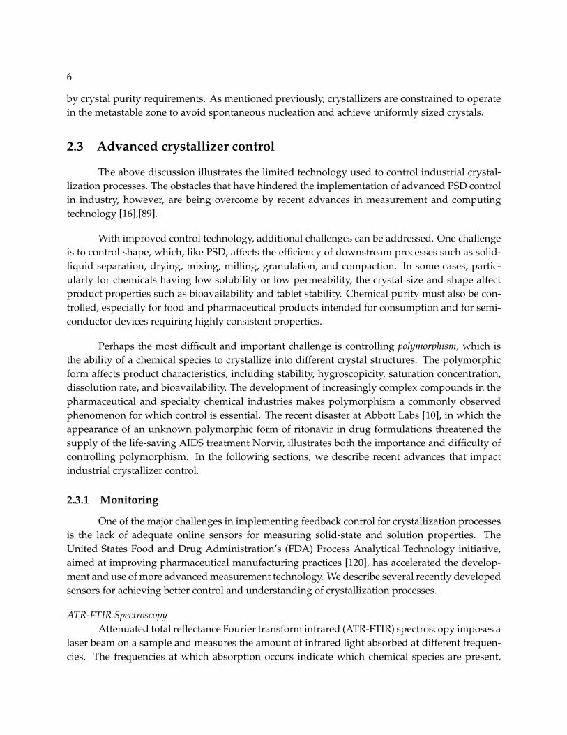
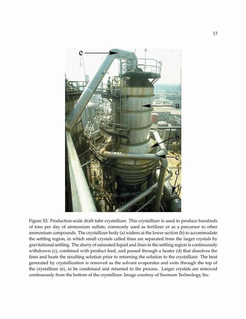
S2 Production-scale draft tube crystallizer. This crystallizer is used to produce hun-dreds of tons per day of ammonium sulfate, commonly used as fertilizer or as aprecursor to other ammonium compounds. The crystallizer body (a) widens at thelower section (b) to accommodate the settling region, in which small crystals calledfines are separated from the larger crystals by gravitational settling. The slurry ofsaturated liquid and fines in the settling region is continuously withdrawn (c), com-bined with product feed, and passed through a heater (d) that dissolves the finesand heats the resulting solution prior to returning the solution to the crystallizer.The heat generated by crystallization is removed as the solvent evaporates and exitsthrough the top of the crystallizer (e), to be condensed and returned to the process.Larger crystals are removed continuously from the bottom of the crystallizer. Imagecourtesy of Swenson Technology, Inc. . . . . . . . . . . . . . . . . . . . . . . . . . . . 13

S3 Production-scale draft tube baffle crystallizer. This crystallizer is used to producehundreds of tons per day of sodium chlorate, which is commonly used in herbi-cides. Image courtesy of Swenson Technology, Inc. . . . . . . . . . . . . . . . . . . . . 14

S4 Small crystallizer used for high potency drug manufacturing. The portal (a) pro-vides access to the crystallizer internals. The crystallizer widens at the lower section(b) to accommodate the crystallizer jacket, to which coolant (e) and heating fluid (h)lines are connected. Mixing is achieved using an impeller driven from below (c).The process feed enters from above (f) and exits below (d). The temperature sensoris inserted from above (g). Image courtesy of Ferro Pfanstiehl Laboratories, Inc. . . . 15

ix

S5 Upper section (top image), lower section (center image), and internals of batch crys-tallizer, showing the impeller and temperature sensor. This crystallizer is used forcontract pharmaceutical and specialty chemical manufacturing. Images courtesy ofAvecia, Ltd. . . . . . . . . . . . . . . . . . . . . . . . . . . . . . . . . . . . . . . . . . . 16

S6 Batch cooling crystallization. In this illustration, the process is cooled until it be-comes supersaturated and crystallization can occur. As the solute species depositonto the forming crystals, the solute concentration decreases. Supersaturation istherefore maintained by further cooling. As shown in (a), a well-controlled crystal-lization process operates in the metastable zone between the saturation concentra-tion and metastable limit, balancing the nucleation and growth rates to achieve thedesired crystal size distribution. As depicted in (b), disturbances such as impuritiescan shift the metastable zone, resulting in undesired nucleation that substantiallydegrades the resulting particle size distribution. . . . . . . . . . . . . . . . . . . . . . 17

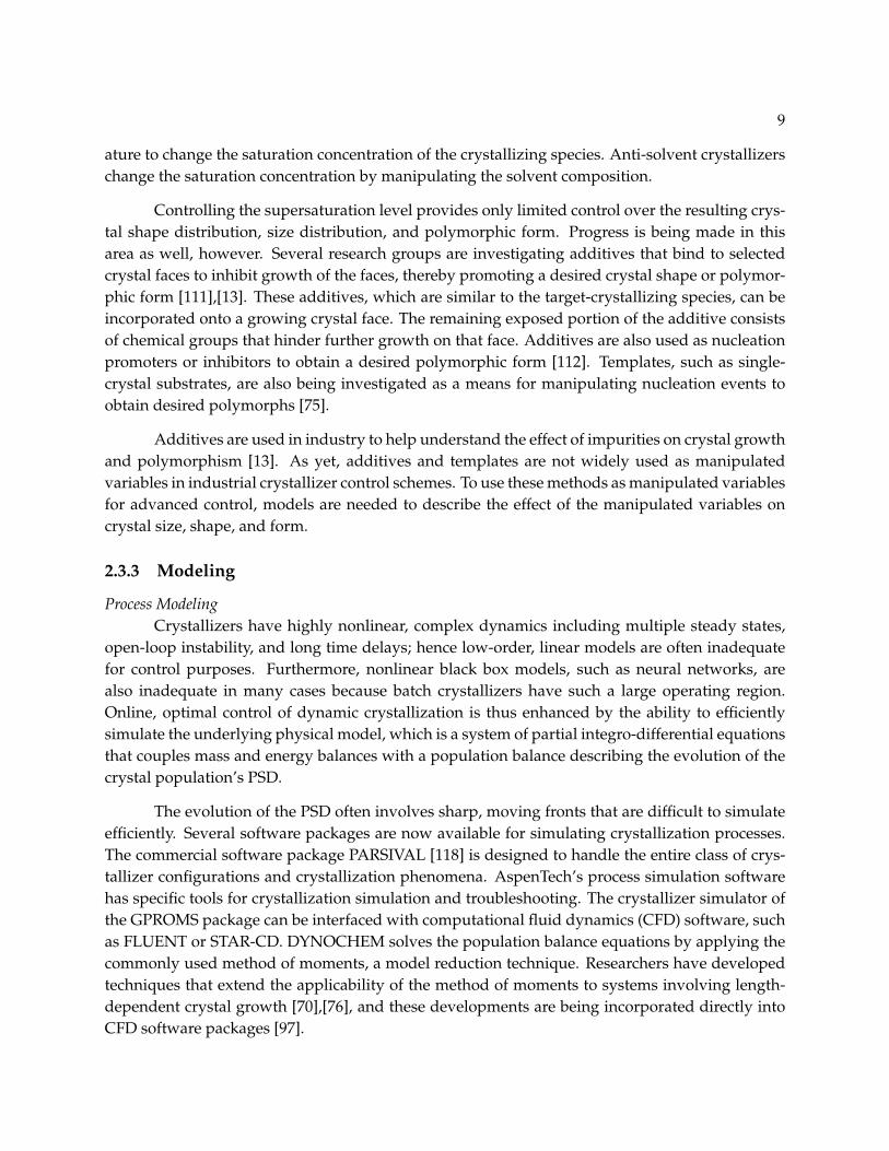
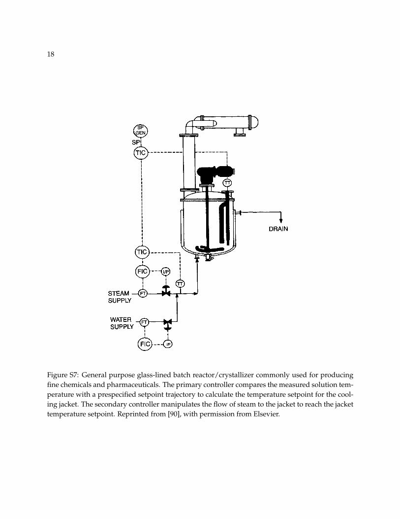
S7 General purpose glass-lined batch reactor/crystallizer commonly used for produc-ing fine chemicals and pharmaceuticals. The primary controller compares the mea-sured solution temperature with a prespecified setpoint trajectory to calculate thetemperature setpoint for the cooling jacket. The secondary controller manipulatesthe flow of steam to the jacket to reach the jacket temperature setpoint. Reprintedfrom [90], with permission from Elsevier. . . . . . . . . . . . . . . . . . . . . . . . . . 18

S8 Comparison of crystal-size measurements obtained using laser backscattering ver-sus those obtained using vision. Laser backscattering provides chord lengths (c1,c2, c3) while vision-based measurement provides projected lengths (l1, l2, l3) andprojected widths (w1, w2, w3). The chord-length measurement for each particle de-pends on its orientation with respect to the laser path (depicted above using the redarrow), while the projected length and width measurements are independent of in-plane orientation. Size measurements from both techniques are affected by particleorientation in depth. . . . . . . . . . . . . . . . . . . . . . . . . . . . . . . . . . . . . . 19

S1 Geometry of the quadratic function . . . . . . . . . . . . . . . . . . . . . . . . . . . . . 27

S1 Experimental setup for obtaining in situ crystallization images. . . . . . . . . . . . . 29

S1 Example of SHARC algorithm applied to an in situ image of suspended pharma-ceutical crystals. (a) A region of interest in the original image. (b) Linear features(ELSs) extracted from the original image. (c) ELSs (black lines) and lines represent-ing each collinear line pair (white lines). (d) Representative rectangles for clusters ofspatially-proximate parallel lines with roughly equal length. The lengths, widths,and aspect ratios of the rectangles are used as the crystal size and shape measure-ments. . . . . . . . . . . . . . . . . . . . . . . . . . . . . . . . . . . . . . . . . . . . . . . 34

x

S2 Depiction of different eight-bucket gradient direction quantizations used to labelpixels. For the quantization on the left, pixels having gradient direction in the rangeof 0 to 45 degrees are labeled as “1”, pixels with gradient direction in the range of 45to 90 degrees are labeled as “2”, and so forth. Quantization effects are mitigated byapplying a second quantization, such as that shown on the right, and subsequentlyresolving any conflicts between the results given by each quantization. . . . . . . . . 35

S3 Example of finding linear features using Burns line finder and blob analysis. (a)Grayscale image. (b) Regions of pixels having similar gradient orientation, deter-mined using the Burns line finder. (c) Best-fit ellipses for each region of pixels,determined using blob analysis. (d) Major axes of the best-fit ellipses imposed onthe original grayscale image. . . . . . . . . . . . . . . . . . . . . . . . . . . . . . . . . . 36

S4 Depiction of variables used in line pair classification scheme. . . . . . . . . . . . . . . 37

S5 Examples of valid and invalid parallel line pairs. The solid lines represent ELSs andthe dotted lines represent base lines (lines arising from instances of collinearity). In(a), the base lines 5 and 6 form a valid parallel pair, and the ELSs 3 and 4 also forma valid parallel pair. In (b), the parallel lines 4 and 5 are an invalid parallel pairbecause they both depend upon ELS 3. Similarly, in (c), base line 3 and ELS 1 forman invalid pair because both depend on ELS 1. . . . . . . . . . . . . . . . . . . . . . . 38

S6 Example of clustering procedure for valid parallel pairs. (a) ELSs (dark) and baselines (light) involved in at least one valid parallel pair. (b) The pair with the highestsignificance. (c) Lines that are parallel-paired (either directly or indirectly) witheither of the lines in the highest significance pair. (d) The bounding box calculatedfor the line cluster. . . . . . . . . . . . . . . . . . . . . . . . . . . . . . . . . . . . . . . . 39

S7 Temperature trajectory for crystallization experiment. The vertical lines indicate thetimes at which sets of video images were acquired. . . . . . . . . . . . . . . . . . . . . 40

S8 Algorithm performance on example image (set 3, frame 1). . . . . . . . . . . . . . . . 42




S12 Comparison of cumulative number fractions obtained from manual and automaticsizing of crystals for video image sets 3, 4, 5, and 6. Set 3 was manually sized bynine different operators. . . . . . . . . . . . . . . . . . . . . . . . . . . . . . . . . . . . 46

S13 Comparison of crystals sized manually (top) and using SHARC (bottom). . . . . . . 47

S14 Zoomed-in view of crystals that SHARC failed to identify correctly. From top tobottom, the crystal labels are two, eleven, and fifteen (according to labels in Fig-ure S13). Column (a): Original image. Column (b): ELS data. Column (c): ELSs andbase lines. Column (d): Result of clustering. . . . . . . . . . . . . . . . . . . . . . . . . 49

S1 Wire-Frame glycine crystal model. The parameters for the model are the crystalbody height, h, the width, w, and the pyramid height, t. . . . . . . . . . . . . . . . . . 54

xi

S2 Depiction of the perspective projection of the glycine model onto the image plane.For simplicity, the image plane is displayed in front of the camera. . . . . . . . . . . . 55

S3 Depiction of different viewpoint-invariant line groups (VIGs) used by M-SHARC.(a) Junction. (b) Parallel pair. (c) Parallel triple. (d) C-triple. (e) C-square. (f) Arrow. 57

S4 Depiction of two correspondence hypotheses. (a) Data line segments. (b) Hypothe-sis 1: Data lines i, j, and k correspond to model edges E1, E9, and E17, respectively.(c) Hypothesis 2: Data lines i, j, and k correspond to model edges E9, E17, and E19,respectively. . . . . . . . . . . . . . . . . . . . . . . . . . . . . . . . . . . . . . . . . . . 58

S5 Depiction of variables used in mismatch calculation for a single line correspondence. 60

S6 Result of applying M-SHARC to image of α-glycine crystal. (a) Original regionof interest. (b) Linear features extracted using Burns line finder (dark lines). (c)Linear features extracted using collinear grouping (light lines). (d) Most salient linegroup. (e) Model initialization. (f) Identification of additional correspondences. (g)Optimized model fit. (h) Invalidated VIGs. . . . . . . . . . . . . . . . . . . . . . . . . 61

S7 M-SHARC segmentation results for selected images acquired at low solids concen-tration (13 min. after appearance of crystals). . . . . . . . . . . . . . . . . . . . . . . . 63

S8 M-SHARC segmentation results for selected images acquired at medium solids con-centration (24 min. after appearance of crystals). . . . . . . . . . . . . . . . . . . . . . 64

S9 M-SHARC segmentation results for selected images acquired at high solids concen-tration (43 min. after appearance of crystals). . . . . . . . . . . . . . . . . . . . . . . . 65

S10 Illustration of comparison between human operator results and M-SHARC results.(a) Original image. (b) Outlines of crystals identified by human operator. (c) Out-lines of crystals identified by M-SHARC. (d) Result of comparison between humanoutlines and M-SHARC outlines. Crystals identified as false positives are outlinedin white while those identified as misses are outlined in black. . . . . . . . . . . . . . 66

S11 Comparison of Human and M-SHARC cumulative distribution functions for pro-jected area. Rows 1, 2, and 3 show results for the α-glycine experiment at low,medium, and high solids concentrations, respectively. Column 1: CDFs constructedusing only crystals classified as hits. Column 2: CDFs constructed using all crystals(i.e. the Human CDF is based on crystals classified as either hit or miss, while theM-SHARC CDF is based on crystals classified as either hit or false positive. . . . . . 69

S12 Results of linear feature detection for selected crystals missed by M-SHARC. Thepoor contrast for the crystals in row 1 is due to out-of-focus blur. The crystals inrow 2 also exhibit poor contrast despite being seemingly in-focus. The crystals inrow 3 show examples of agglomeration. The crystals in row 4 may be identifiablegiven further development of M-SHARC’s correspondence and model parameterestimation routines described in Sections 6.2.4 and 6.2.4. . . . . . . . . . . . . . . . . 70

S1 Depiction of methodology for calculating Miles-Lantuejoul M-values for particlesof different lengths observed in an image of dimension b× a. . . . . . . . . . . . . . . 73

xii

S2 Depiction of the perspective projection of a cylindrical particle onto the image plane.For simplicity, the image plane is displayed in front of the camera. . . . . . . . . . . . 79

S3 Depiction of CCD image. . . . . . . . . . . . . . . . . . . . . . . . . . . . . . . . . . . . 79S4 Example images for simulations of various particle populations. Row 1: monodis-

perse particles of length 0.5a, Nc=25. Row 2: particles uniformly distributed on[0.1a 0.9a]. Row 3: particles normally-distributed with µ = 0.5a and σ = 0.4a/3,Nc=25. Row 4: particles uniformly-distributed on [0.1a 2.0a], Nc=15. . . . . . . . . . 81

S5 Comparison of estimated sampling distributions for absolute PSD for monodis-perse particles. Results based on 1000 simulations, 10 size classes, Nc=25. (a) Re-sults for 10 images/simulation. (b) Results for 100 images/simulation. . . . . . . . . 82

S6 Fraction of confidence intervals containing the true parameter value versus confi-dence level. Results based on 1000 simulations, 10 size classes (results shown onlyfor size class corresponding to monodisperse particle size), Nc = 25. (a) Results for10 images/simulation. (b) Results for 100 images/simulation. . . . . . . . . . . . . . 83

S7 Relative efficiencies (eff(ρbi, ρMLi)) plotted versus size class for various numbers of

images per simulation: case study 2. . . . . . . . . . . . . . . . . . . . . . . . . . . . . 84S8 Fraction of confidence intervals containing true parameter values for different con-

fidence levels, N=100. (a) Size class 1 (smallest size class). (b) Size class 4. (c) Sizeclass 7. (d) Size class 10 (largest size class). . . . . . . . . . . . . . . . . . . . . . . . . . 85

S9 Fraction of confidence intervals containing true parameter values for different con-fidence levels, N=10. (a) Size class 1 (smallest size class). (b) Size class 4. (c) Sizeclass 7. (d) Size class 10 (largest size class). . . . . . . . . . . . . . . . . . . . . . . . . . 86

S10 Sampling distributions for the various size classes of a discrete normal distribution.N = 100. . . . . . . . . . . . . . . . . . . . . . . . . . . . . . . . . . . . . . . . . . . . . 87

S11 Relative efficiencies (eff(ρbi, ρMLi)) plotted versus size class for various numbers of

images per simulation: case study 3. . . . . . . . . . . . . . . . . . . . . . . . . . . . . 88S12 Comparison of sampling distributions for absolute PSD for particles distributed

uniformly on [0.4a 2.0a]. Results based on 200 simulations, 100 images/simulation,10 size classes, Nc=15. (a) Size class 1. (b) Size class 5. (c) Size class 9. (d) Size class10. (e) Lmax. . . . . . . . . . . . . . . . . . . . . . . . . . . . . . . . . . . . . . . . . . . 88

S1 Geometric representation of region in which particles of specific orientation andshape overlap. . . . . . . . . . . . . . . . . . . . . . . . . . . . . . . . . . . . . . . . . . 94

S2 Depiction of the perspective projection of a cylindrical particle onto the image plane.For simplicity, the image plane is displayed in front of the camera. . . . . . . . . . . . 96

S3 Depiction of CCD image. . . . . . . . . . . . . . . . . . . . . . . . . . . . . . . . . . . . 97S4 Comparison of images generated for two different monodisperse particle popula-

tions at the same solids concentration MT and at the same D. The top row showsthe images for particles with length 1/20th of the image dimension and the bot-tom row shows images for particles with length one-half the image dimension. Theaspect ratio of the particles is 10. . . . . . . . . . . . . . . . . . . . . . . . . . . . . . . 99

xiii

S5 Comparison of average number of overlaps per crystal for images simulated at con-stant D and at constants solids concentration for monodisperse populations of var-ious crystal sizes. . . . . . . . . . . . . . . . . . . . . . . . . . . . . . . . . . . . . . . . 99

S6 Comparison of percentage of particles missed by automated image analysis for im-ages simulated at constant D and at constants solids concentration for monodis-perse populations of various crystal sizes. . . . . . . . . . . . . . . . . . . . . . . . . . 100

S7 Examples of synthetic images generated at various D. The first, second, and thirdcolumn correspond to particle sizes L/a = 0.1, 0.3, and 0.5, respectively. . . . . . . . . 101

S8 Results of number density estimation using Miles-Lantuejoul method for variousparticle sizes and various levels of image difficulty. (a) Results for applying Miles-Lantuejoul method directly to image analysis output. (b) Results for empirical cor-rection of the Miles-Lantuejoul estimate based on estimated value of D. . . . . . . . 102

S9 Optimal fit for model of number of particles identified per image by automatedimage analysis. Also shown is the ideal model, or the expected number of isolatedparticles predicted for θ = 1 and the number of isolated particles observed in thesimulated images (ideal data). (a) L/a = 0.1, θ = 0.4; (b) L/a = 0.3, θ = 0.3; (c)L/a = 0.5, θ = 0.3. . . . . . . . . . . . . . . . . . . . . . . . . . . . . . . . . . . . . . . . 103

S10 Ratio of estimated density and true density versus image difficulty using SHARCdata and empirical correction factors calculated for each different particle size. . . . 104

S11 Likelihood of observing n non-overlapping particles with example images at lowand high number densities giving the same number of non-overlapping particles.Overlapping particles appear gray while non-overlapping particles appear white. . 105

S1 Depiction of hypothetical system of vertically-oriented particles randomly and uni-formly distributed in space. . . . . . . . . . . . . . . . . . . . . . . . . . . . . . . . . . 110

S2 Depiction of geometrical properties used to derive the non-border area functionAnb(l, θ). . . . . . . . . . . . . . . . . . . . . . . . . . . . . . . . . . . . . . . . . . . . . 111

S3 Depiction of hypothetical system of vertically-oriented particles randomly and uni-formly distributed in space. . . . . . . . . . . . . . . . . . . . . . . . . . . . . . . . . . 113

S4 Depiction of non-border area for arbitrary length and orientation. . . . . . . . . . . . 114

S5 Example images for simulations of various particle populations. Row 1: monodis-perse particles of length 0.5a, Nc=25. Row 2: particles uniformly distributed on[0.1a 0.9a]. Row 3: particles normally-distributed with µ = 0.5a and σ = 0.4a/3with Nc=25. Row 4: particles uniformly-distributed on [0.1a 2.0a], Nc=15. . . . . . . 117

S6 Comparison of theoretical and simulated marginal densities for randomly-oriented,monodisperse particles of length 0.5 and measured by partitioning [0.1 0.9] into tenbins. Results are for non-border particles. . . . . . . . . . . . . . . . . . . . . . . . . . 118

S7 Comparison of theoretical and simulated marginal densities for randomly-oriented,monodisperse particles of length 0.5 and measured by partitioning [0.1 0.9] into tenbins. Results are for border particles. . . . . . . . . . . . . . . . . . . . . . . . . . . . . 118

xiv

S8 Comparison of theoretical and simulated marginal densities for randomly-orientedparticles distributed uniformly on [0.1 0.9] and measured by partitioning [0.1 0.9]into ten bins. Results are for non-border particles. . . . . . . . . . . . . . . . . . . . . 119

S9 Comparison of theoretical and simulated marginal densities for randomly-orientedparticles distributed uniformly on [0.1 0.9] and measured by partitioning [0.1 0.9]into ten bins. Results are for border particles. . . . . . . . . . . . . . . . . . . . . . . . 120

S10 Comparison of theoretical and simulated marginal densities for randomly-orientedparticles distributed normally and measured by partitioning [0.1 0.9] into 10 bins.Results are for non-border particles. . . . . . . . . . . . . . . . . . . . . . . . . . . . . 121

S11 Comparison of theoretical and simulated marginal densities for randomly-orientedparticles distributed normally and measured by partitioning [0.1 0.9] into 10 bins.Results are for border particles. . . . . . . . . . . . . . . . . . . . . . . . . . . . . . . . 122

S12 Comparison of theoretical and simulated marginal densities for randomly-orientedparticles distributed uniformly on [0.4 2.0] and measured by partitioning [0.4 1.0]into 9 bins with a 10th bin spanning [1.0

√2]. Results are for non-border particles. . 123

S13 Comparison of theoretical and simulated marginal densities for randomly-orientedparticles distributed uniformly on [0.4 2.0] and measured by partitioning [0.4 1.0]into 9 bins with a 10th bin spanning [1.0

√2]. Results are for border particles. . . . . 124

1

Chapter 1

Introduction1.1 Crystallization overview

Crystallization plays a critical role in numerous industries for a variety of reasons. In thesemiconductor industry, for example, crystallization is used to grow long, cylindrical, single crys-tals of silicon with a mass of several hundred kilograms. These gigantic crystals, called boules, aresliced into thin wafers upon which integrated circuits are etched. Prior to etching, crystallizationis used to grow thin layers of crystalline, semiconductor material onto the silicon wafer using aprocess called chemical vapor deposition. In the food industry, crystallization is often used togive products the right texture, flavor, and shelf life. Crystallization is used to produce ice cream,frozen dried foods, chewing gum, butter, chocolate, salt, cheese, coffee, and bread [46]. Theseexamples highlight the utility of crystallization in creating solids with desirable and consistentproperties.

Crystallization is also widely used to separate and purify chemical species in the com-modity, petrochemical, specialty, and fine-chemical industries. In fact, DuPont, one of the world’slargest chemical manufacturers, estimated in 1988 [42] that approximately 70% of its products passthrough a crystallization or precipitation stage.

Crystallization is a critical process for the pharmaceutical industry. The vast majority ofpharmaceuticals are manufactured in solid, generally crystalline, form. Crystallization is usedto identify structure for use in drug design, to isolate chemical species from mixtures of reactionproducts, and to achieve consistent and controlled drug delivery.

Although each of the industries mentioned above is important to the U.S. economy, gener-ating 35% of the United States’ gross domestic product in 2003, the semiconductor and pharma-ceutical industries are particularly critical to the U.S. economy. Semiconductor Industry Associa-tion (SIA) President George Scalise stated in the SIA 2004 Annual Report that “the U.S. economy ishardwired to semiconductor innovation.” After suffering severe setbacks in 2001, the semiconduc-tor industry rebounded and is expected to maintain 8 to 10 percent growth in the coming years.According to the SIA, worldwide semiconductor sales in 2004 exceeded USD$213 billion, with theU.S. gaining nearly 47% of the market [98]. A 2004 study conducted by the Milken Institute [73]found that the biopharmaceutical industry directly employed over 400,000 people in 2003 whilegenerating 2.3 million additional jobs, making it responsible for over 2 percent of the total em-ployment in the United States. The study found furthermore that the biopharmaceutical industry

2

generated USD$115 billion dollars in total workers’ earnings in 2003, including USD$29.5 billiondirect impact (pharmaceutical company employees), USD$54.3 billion indirect impact (employeesof related companies, such as raw material suppliers or vendors), and USD$31.3 billion inducedimpact (employment as a result of direct and indirect spending).

Given the widespread use of crystallization in these industries, achieving good controlover crystallization processes is clearly an economically significant goal. In this article, we explainhow crystallization is controlled in industrial processes and what challenges must be overcome toachieve better control.

1.2 Thesis overview

3

Chapter 2

Literature review2.1 Crystallization tutorial

Crystallization is the formation of a solid state of matter in which the molecules are arranged ina regular pattern. Crystallization can be carried out by a variety of methods, but the conceptsand terminology relevant to most crystallization processes can be understood by examining themethod of solution crystallization. In solution crystallization, the physical system consists of oneor more solutes dissolved in a solvent. The system can be undersaturated, saturated, or supersatu-rated with respect to species i, depending on whether the solute concentration ci is less than, equalto, or greater than the saturation concentration c∗i . Crystallization occurs only if the system is super-saturated. The supersaturation level is the amount by which the solute concentration exceeds thesaturation concentration, and is commonly expressed as σ = ci−c∗i

c∗i, S = ci

c∗i, or ∆c = ci − c∗i . The

supersaturation level can be increased either by lowering the saturation concentration (for exam-ple, by cooling as depicted in Figure S1) or by increasing the solute concentration (by evaporatingthe solvent, for example).

Crystallization moves a supersaturated solution toward equilibrium by transferring solutemolecules from the liquid phase to the solid, crystalline phase. This process is initiated by nucle-ation, which is the birth or initial formation of a crystal. Nucleation occurs, however, only if thenecessary activation energy is supplied. A supersaturated solution in which the activation energyis too high for nucleation to occur is called metastable. As the supersaturation level increases, theactivation energy decreases. Thus spontaneous nucleation, also called primary nucleation, occursonly at sufficiently high levels of supersaturation, and the solute concentration at which this nu-cleation occurs is called the metastable limit. Since primary nucleation is difficult to control reliably,primary nucleation is often avoided by injecting crystal seeds into the supersaturated solution.

Crystal nuclei and seeds provide a surface for crystal growth to occur. Crystal growthinvolves solute molecules attaching themselves to the surfaces of the crystal according to the crys-talline structure. Crystals suspended in a well-mixed solution can collide with each other or withthe crystallizer internals, causing crystal attrition and breakage that results in additional nuclei.Nucleation of this type is called secondary nucleation.

The rates at which crystal nucleation and growth occur are functions of the supersatura-tion level. The goal of crystallizer control is to balance the nucleation and growth rates to achieve

4

the desired crystal size objective. Often, the size objective is to create large, uniformly sized crys-tals. Well-controlled crystallization processes operate in the metastable zone, between the saturationconcentration and the metastable limit, to promote crystal growth while minimizing undesirablenucleation.

2.2 Crystallization process control in industry

The objective of every industrial crystallization process is to create crystals that meet spec-ifications on size, shape, composition, and internal structure. This objective is achieved using avariety of methods and equipment configurations depending on the properties of the chemicalsystem, the end-product specifications, and the production scale. Continuous crystallizers, suchas those shown in Figures S2 and S3, are typically used for large-scale production, producinghundreds of tons per day. In the specialty chemical, fine chemical, and pharmaceutical industries,batch crystallizers (see figures S4 and S5) are often used to produce low-volume, high-value-addedchemicals.

2.2.1 Process development

The first step in developing a control system for solution crystallization is to determine thesaturation concentration and metastable limit of the target species over a range of temperatures,solvent compositions, and pH’s. The saturation concentration, also called solubility, representsthe minimum solute concentration for which crystal growth can occur. The metastable limit, onthe other hand, indicates the concentration above which undesirable spontaneous nucleation oc-curs (see the “Crystallization tutorial” sidebar). Spontaneous nucleation, which yields smaller,non-uniform crystals, can be avoided by injecting crystal “seeds” into the crystallizer to initial-ize crystal growth. The saturation concentration and metastable limit provide constraints on theoperating conditions of the process and determine the appropriate crystallization method. For ex-ample, chemical systems in which the solubility is highly sensitive to temperature are crystallizedusing cooling, while systems with low solubility temperature dependence employ anti-solvent orevaporation crystallization. Automation tools greatly reduce the amount of time, labor, and mate-rial previously required to characterize the solubility and metastable limit, enabling a wide rangeof conditions to be tested in a parallel fashion [11].

Once a crystallization method and solvents are chosen, kinetic studies are carried out on alarger scale (tens to hundreds of milliliters) to characterize crystal growth and nucleation rates andto develop an operating policy (see Figure S6) that is robust to variations in mixing, seeding, andimpurity levels. These studies minimize the difficulty in scaling up the process several orders ofmagnitude to the pilot scale. The operating policy is usually determined semi-quantitatively, us-ing trial-and-error or statistical-design-of-experiment approaches. Process robustness is achievedby adopting a conservative operating policy at low supersaturation levels that minimize nucle-ation events and thus achieve larger, more uniform crystals. Operating at low supersaturation

5

levels, far from the metastable limit, is important because the metastable limit is difficult to char-acterize and is affected by various process conditions that change upon scaleup, such as the sizeand type of vessel or impeller.

2.2.2 Controlled, measured, and manipulated variables

The primary concern of most industrial crystallization processes is generating crystals witha particle size distribution (PSD) that enables efficient downstream processing. The controlledvariable for most crystallization processes, however, is the supersaturation level, which is onlyindirectly related to the PSD. The supersaturation level affects the relative rates of nucleation andgrowth and thus determines the PSD. Because of its dependence on temperature and solutioncomposition, the supersaturation level can be manipulated using various process variables suchas the flow rate of the cooling medium to the crystallizer jacket and the flow rate of anti-solvent tothe crystallizer.

Process development studies use a wide range of measurement technology. This technol-ogy includes, for example, turbidity probes to detect the presence of solid material, laser scatter-ing to characterize particle size distributions, and spectroscopic or absorbance probes to measuresolute concentrations. However, large-scale, industrial crystallizers rarely have these advancedmeasurements available. In fact, controllers for most industrial crystallizers rely primarily on tem-perature, pressure, and flow rate measurements. For example, Figure S7 illustrates a commonlyused cascade control strategy that uses temperature feedback to follow a prespecified temperaturetrajectory. This control system is clearly not robust to deviations from the temperature trajectoryor disturbances affecting the saturation concentration and metastable limit, as depicted in Fig-ure S6(b).

2.2.3 Nonlinearities and constraints

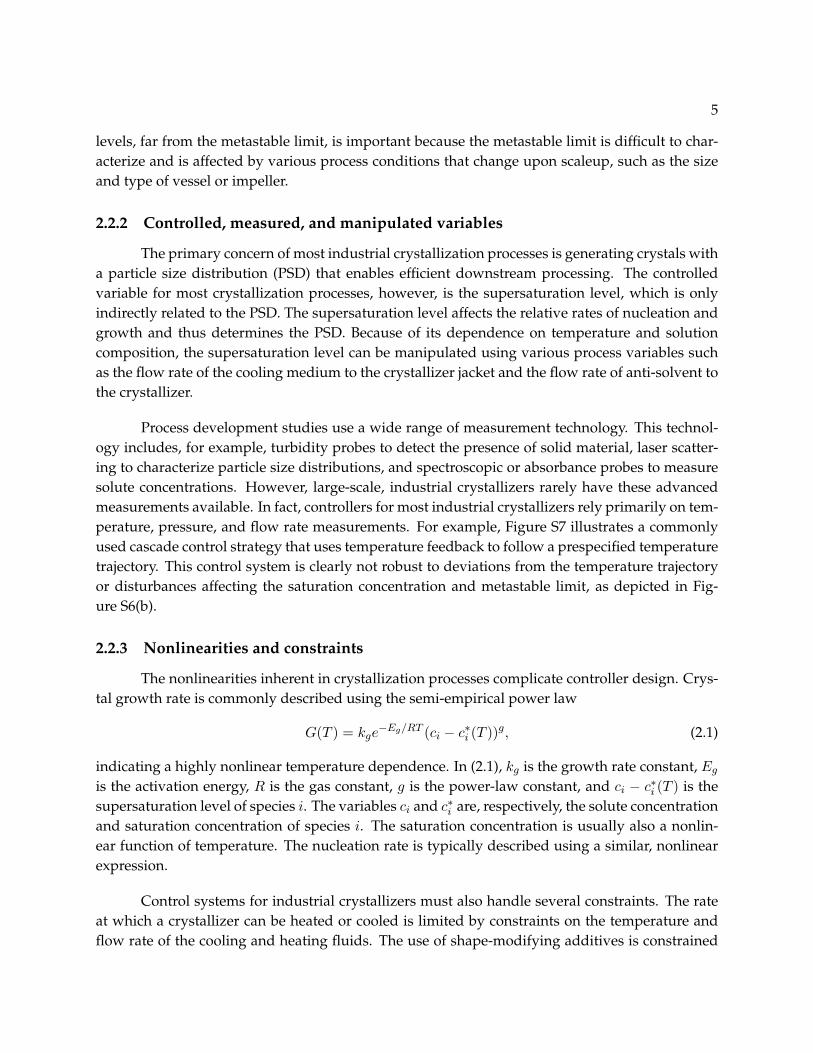
The nonlinearities inherent in crystallization processes complicate controller design. Crys-tal growth rate is commonly described using the semi-empirical power law

G(T ) = kge−Eg/RT (ci − c∗i (T ))g, (2.1)

indicating a highly nonlinear temperature dependence. In (2.1), kg is the growth rate constant, Eg

is the activation energy, R is the gas constant, g is the power-law constant, and ci − c∗i (T ) is thesupersaturation level of species i. The variables ci and c∗i are, respectively, the solute concentrationand saturation concentration of species i. The saturation concentration is usually also a nonlin-ear function of temperature. The nucleation rate is typically described using a similar, nonlinearexpression.

Control systems for industrial crystallizers must also handle several constraints. The rateat which a crystallizer can be heated or cooled is limited by constraints on the temperature andflow rate of the cooling and heating fluids. The use of shape-modifying additives is constrained

6

by crystal purity requirements. As mentioned previously, crystallizers are constrained to operatein the metastable zone to avoid spontaneous nucleation and achieve uniformly sized crystals.

2.3 Advanced crystallizer control

The above discussion illustrates the limited technology used to control industrial crystal-lization processes. The obstacles that have hindered the implementation of advanced PSD controlin industry, however, are being overcome by recent advances in measurement and computingtechnology [16],[89].

With improved control technology, additional challenges can be addressed. One challengeis to control shape, which, like PSD, affects the efficiency of downstream processes such as solid-liquid separation, drying, mixing, milling, granulation, and compaction. In some cases, partic-ularly for chemicals having low solubility or low permeability, the crystal size and shape affectproduct properties such as bioavailability and tablet stability. Chemical purity must also be con-trolled, especially for food and pharmaceutical products intended for consumption and for semi-conductor devices requiring highly consistent properties.

Perhaps the most difficult and important challenge is controlling polymorphism, which isthe ability of a chemical species to crystallize into different crystal structures. The polymorphicform affects product characteristics, including stability, hygroscopicity, saturation concentration,dissolution rate, and bioavailability. The development of increasingly complex compounds in thepharmaceutical and specialty chemical industries makes polymorphism a commonly observedphenomenon for which control is essential. The recent disaster at Abbott Labs [10], in which theappearance of an unknown polymorphic form of ritonavir in drug formulations threatened thesupply of the life-saving AIDS treatment Norvir, illustrates both the importance and difficulty ofcontrolling polymorphism. In the following sections, we describe recent advances that impactindustrial crystallizer control.

2.3.1 Monitoring

One of the major challenges in implementing feedback control for crystallization processesis the lack of adequate online sensors for measuring solid-state and solution properties. TheUnited States Food and Drug Administration’s (FDA) Process Analytical Technology initiative,aimed at improving pharmaceutical manufacturing practices [120], has accelerated the develop-ment and use of more advanced measurement technology. We describe several recently developedsensors for achieving better control and understanding of crystallization processes.

ATR-FTIR SpectroscopyAttenuated total reflectance Fourier transform infrared (ATR-FTIR) spectroscopy imposes a

laser beam on a sample and measures the amount of infrared light absorbed at different frequen-cies. The frequencies at which absorption occurs indicate which chemical species are present,

7

while the absorption magnitudes indicate the concentrations of these species. As demonstratedin [30] and [29], ATR-FTIR spectroscopy can be used to monitor solute concentration in a crystal-lization process in situ.

ATR-FTIR spectroscopy offers advantages over prior techniques, such as refractometry,densitometry, and conductivity measurements, for measuring solute concentration. Refractom-etry works only if there is a significant change in the refractive index with solute concentrationand is sensitive to air bubbles. Densitometry requires sampling of the crystal slurry and filteringout the crystals to accurately measure the liquid-phase density. This sampling process involvesan external loop that is sensitive to temperature fluctuations and subject to filter clogging. Con-ductivity measurements, which are useful only for electrolytes, require frequent re-calibration.ATR-FTIR spectroscopy overcomes these problems and can measure multiple solute concentra-tions. Calibration of ATR-FTIR is usually rapid [62] and thus well suited for batch processes andshort production runs. In [105], linear chemometrics is applied to estimate solute concentrationwith high accuracy (within 0.12%). Several applications for which ATR-FTIR monitoring is usefulare described in [34].

Unfortunately, ATR-FTIR spectroscopy is considerably more expensive than the alterna-tives. Another drawback of ATR-FTIR is the vulnerability of the IR probe’s optical material tochemical attack and fouling [28].

Raman spectroscopyRaman spectroscopy imposes a monochromatic laser beam on a sample and measures the

amount of light scattered at different wavelengths. The differences in wavelength between theincident light and the scattered light is a fingerprint for the types of chemical bonds in the sample.Raman spectroscopy has been used to make quantitative polymorphic composition measurementssince 1991 [25]. This technology has been applied to quantitative, in situ polymorphic compositionmonitoring in solution crystallization since 2000 [110]–[79].

Raman spectroscopy is well suited to in situ polymorphism monitoring for several rea-sons. Specifically, Raman analysis does not require sample preparation; the Raman signal can bepropagated with fiber optics for remote sensing; and Raman sampling probes are less chemicallysensitive than ATR-FTIR probes [28]. In addition, this technique can be used to monitor the solidand liquid phases simultaneously [32],[49].

Like ATR-FTIR, Raman-based technologies are expensive. Furthermore, calibration of theRaman signal for quantitative polymorphic composition measurements can be difficult becausethe signal intensity is affected by the particle size distribution. Hence Raman’s utility for quanti-tative monitoring depends on corrections for particle-size effects [81].

Near-Infrared SpectroscopyNear-infrared (NIR) spectroscopy is also used to quantitatively monitor polymorphic com-

position [78]. Like Raman, NIR is well suited for in situ analysis. The main drawback of NIR is that

8

calibration is difficult and time consuming. In some cases, however, coarse calibration is sufficientto extract the needed information [35].

Laser backscatteringLaser backscattering-based monitoring technology, such as Lasentec’s FBRM probe, has

proven useful for characterizing particle size and for determining saturation concentrations andmetastable limits [8],[9]. This sensor measures particle chord lengths (see Figure S8) by movinga laser beam at high velocity through the sample and recording the crossing times, that is, thetime durations over which light is backscattered as the laser passes over particles. The chordlength of each particle traversed by the laser is calculated as the product of the laser’s velocityand the crossing time of the particle. This technique allows rapid, calibration-free acquisition ofthousands of chord-length measurements to robustly construct a chord length distribution (CLD).Laser backscattering technology can be applied in situ under high solids concentrations.

Because laser-backscattering provides a measurement of only chord length, this techniquecannot be used to measure particle shape directly. Also, inferring the PSD from the CLD involvesthe solution of an ill-posed inversion problem. Although methods for solving this inversion prob-lem are developed in [63],[116], these methods depend on assumptions regarding particle shape.CLD thus provides only a qualitative indication of the underlying PSD characteristics.

Video MicroscopyVideo microscopy can be used to characterize both crystal size and shape. Furthermore, for

chemical systems in which the polymorphs exhibit different shapes, such as glycine in water, videomicroscopy can be used to monitor polymorphic composition [18]. Obtaining all three of thesemeasurements using a single probe reduces cost and simplifies the experimental setup. Videomicroscopy is also appealing because interpretation of image data is intuitive.

Several challenges associated with video microscopy have limited its application for parti-cle size and shape analysis. Most commercial video-microscopy-based analyzers require samplingto obtain images for automatic image analysis. Although in situ probes are available, their util-ity has mainly been limited to qualitative monitoring because the nature of the images, whichcontain blurred, out-of-focus, and overlapping particles, precludes the successful application ofimage analysis to automatically quantify particle size and shape. Furthermore, crystal-size mea-surements obtained from images depend on the orientation of the crystals with respect to thecamera, although the effect is less pronounced than for laser backscattering-based measurements(see Figure S8).

2.3.2 Manipulated variables

In advanced control implementations, the quality variables of interest (crystal size, shape,form, and purity) are indirectly controlled using manipulated variables that affect the supersatura-tion level in the crystallizer. For example, cooling crystallizers manipulate the crystallizer temper-

9

ature to change the saturation concentration of the crystallizing species. Anti-solvent crystallizerschange the saturation concentration by manipulating the solvent composition.

Controlling the supersaturation level provides only limited control over the resulting crys-tal shape distribution, size distribution, and polymorphic form. Progress is being made in thisarea as well, however. Several research groups are investigating additives that bind to selectedcrystal faces to inhibit growth of the faces, thereby promoting a desired crystal shape or polymor-phic form [111],[13]. These additives, which are similar to the target-crystallizing species, can beincorporated onto a growing crystal face. The remaining exposed portion of the additive consistsof chemical groups that hinder further growth on that face. Additives are also used as nucleationpromoters or inhibitors to obtain a desired polymorphic form [112]. Templates, such as single-crystal substrates, are also being investigated as a means for manipulating nucleation events toobtain desired polymorphs [75].

Additives are used in industry to help understand the effect of impurities on crystal growthand polymorphism [13]. As yet, additives and templates are not widely used as manipulatedvariables in industrial crystallizer control schemes. To use these methods as manipulated variablesfor advanced control, models are needed to describe the effect of the manipulated variables oncrystal size, shape, and form.

2.3.3 Modeling

Process ModelingCrystallizers have highly nonlinear, complex dynamics including multiple steady states,

open-loop instability, and long time delays; hence low-order, linear models are often inadequatefor control purposes. Furthermore, nonlinear black box models, such as neural networks, arealso inadequate in many cases because batch crystallizers have such a large operating region.Online, optimal control of dynamic crystallization is thus enhanced by the ability to efficientlysimulate the underlying physical model, which is a system of partial integro-differential equationsthat couples mass and energy balances with a population balance describing the evolution of thecrystal population’s PSD.

The evolution of the PSD often involves sharp, moving fronts that are difficult to simulateefficiently. Several software packages are now available for simulating crystallization processes.The commercial software package PARSIVAL [118] is designed to handle the entire class of crys-tallizer configurations and crystallization phenomena. AspenTech’s process simulation softwarehas specific tools for crystallization simulation and troubleshooting. The crystallizer simulator ofthe GPROMS package can be interfaced with computational fluid dynamics (CFD) software, suchas FLUENT or STAR-CD. DYNOCHEM solves the population balance equations by applying thecommonly used method of moments, a model reduction technique. Researchers have developedtechniques that extend the applicability of the method of moments to systems involving length-dependent crystal growth [70],[76], and these developments are being incorporated directly intoCFD software packages [97].

10

Shape ModelingModels and methods for predicting crystal shape based solely on knowledge of the internal

crystal structure are available in software packages such as CERIUS2 and HABIT [22]. These meth-ods provide accurate shape predictions for vapor-grown crystals but, for solution-grown crystals,do not take into account the effects of supersaturation, temperature, solvent, and additives orimpurities. Current shape-modeling research is focused on accounting for these effects [114]–[93].

Polymorphism ModelingThe ability to predict the crystal structure for a given molecule in a given environment

would represent a major advance in drug development. Although significant progress has beenmade in making these predictions [87],[24], this problem is far from being solved. Most ap-proaches seek to find the crystal structure that corresponds to the global minimum in lattice en-ergy, that is, the most thermodynamically stable form at zero Kelvin. These approaches neglectentropic contributions arising at higher temperatures as well as kinetic effects due to the experi-mental crystallization conditions. Current polymorphism modeling methods thus cannot reliablypredict the polymorphs that are observed experimentally.

2.3.4 Control

The developments described above impact the way crystallizer control is approached inindustry. In particular, the development of better measurement technology enables the appli-cation of simple but effective crystallizer control strategies. Most of these strategies focus onfeedback control of supersaturation using concentration (by means of ATR-FTIR) and tempera-ture measurements to follow a predefined supersaturation trajectory [64]–[38]. This approach isattractive because it can be implemented without characterizing the nucleation and growth kinet-ics, using only the saturation concentration and metastable zone width data. Furthermore, thisapproach results in a temperature profile that can be used in large-scale crystallizers that do nothave concentration-measurement capabilities.

Laser backscattering measurements are used to control the number of particles in the sys-tem [27]. This control strategy alternates between cooling and heating stages, allowing the heatingstage to continue until the particle count number measured by FBRM returns to its original valueupon seeding, indicating that all fine particles generated by secondary nucleation have been dis-solved. In [84], online crystal shape measurements obtained by means of optical microscopy andautomated image processing are used to manipulate impurity concentration and thereby con-trol crystal habit. The control schemes employed in these experimental studies are basic (usuallyPID or on-off control), illustrating that, given adequate measurement technology, simple controlschemes can often provide an adequate level of control capability.

More sophisticated control methods have also been demonstrated for batch crystallizers.Experimental results obtained in [74]–[117] demonstrate product improvement by using predic-tive, first-principles models to determine open-loop, optimal cooling and seeding policies. Closed-loop, optimal control of batch crystallizers is demonstrated using simulations in [92],[100].

11

For continuous crystallizers, various model-based, feedback controllers have been sug-gested. In [109], an H∞ controller based on a linearized distributed parameter model is shownto successfully stabilize oscillations in a simulated, continuous crystallizer using measurementsof the overall crystal mass, with the flow rate of fines (small crystals) to the dissolution unit asthe manipulated variable. In [100], a hybrid controller combining model predictive control with abounded controller is used to ensure closed-loop stability for continuous crystallizers.

2.4 The future of crystallization

As the chemical, pharmaceutical, electronics, and food industries continue to develop newproducts, crystallization will enjoy increasingly wide application as a means to separate and pu-rify chemical species and create solids with desirable properties. Sensor technology for crystalliz-ers will continue to improve, especially given the current emphasis by the FDA’s Process Analyt-ical Technology initiative. Industries that have used batch crystallizers to produce low-volume,high-value-added chemicals might choose to move to continuous crystallizers to reduce operatingcosts and enable more flexible and compact process design. Shape modeling and molecular mod-eling tools offer tremendous potential for enabling robust process design and control, and thesetools can be expected to advance rapidly given the amount of interest and research in this area.These developments will impact the way in which crystallization processes are designed and willenable more effective control of size distribution, shape, and polymorphic form, leading to thecreation of crystalline solids that are useful for a wide variety of applications.

12

Solu

teco

ncen

trat

ion

c i

ci < c∗i

Concentration, c∗i (T )Saturation

Temperature T

Metastable limit

Metastable zone

D

ABC

∆ci

B C DA

ci >> c∗i ci = c∗ici > c∗i

Figure S1: Depiction of a cooling, solution crystallization process. The process begins at pointA, at which the solution is undersaturated with respect to species i (ci < c∗i ). The process iscooled to point B, at which the solution is supersaturated (ci > c∗i ). No crystals form at point B,however, because the activation energy for nucleation is too high. As the process cools further,the supersaturation level increases and the activation energy for nucleation decreases. At themetastable limit (point C), spontaneous nucleation occurs, followed by crystal growth. The soluteconcentration decreases as solute molecules are transferred from the liquid phase to the growingcrystals until equilibrium is reached at point D, at which ci = c∗i .

13

Figure S2: Production-scale draft tube crystallizer. This crystallizer is used to produce hundredsof tons per day of ammonium sulfate, commonly used as fertilizer or as a precursor to otherammonium compounds. The crystallizer body (a) widens at the lower section (b) to accommodatethe settling region, in which small crystals called fines are separated from the larger crystals bygravitational settling. The slurry of saturated liquid and fines in the settling region is continuouslywithdrawn (c), combined with product feed, and passed through a heater (d) that dissolves thefines and heats the resulting solution prior to returning the solution to the crystallizer. The heatgenerated by crystallization is removed as the solvent evaporates and exits through the top ofthe crystallizer (e), to be condensed and returned to the process. Larger crystals are removedcontinuously from the bottom of the crystallizer. Image courtesy of Swenson Technology, Inc.

14

Figure S3: Production-scale draft tube baffle crystallizer. This crystallizer is used to produce hun-dreds of tons per day of sodium chlorate, which is commonly used in herbicides. Image courtesyof Swenson Technology, Inc.

15

Figure S4: Small crystallizer used for high potency drug manufacturing. The portal (a) providesaccess to the crystallizer internals. The crystallizer widens at the lower section (b) to accommodatethe crystallizer jacket, to which coolant (e) and heating fluid (h) lines are connected. Mixing isachieved using an impeller driven from below (c). The process feed enters from above (f) and exitsbelow (d). The temperature sensor is inserted from above (g). Image courtesy of Ferro PfanstiehlLaboratories, Inc.

16

Figure S5: Upper section (top image), lower section (center image), and internals of batch crystal-lizer, showing the impeller and temperature sensor. This crystallizer is used for contract pharma-ceutical and specialty chemical manufacturing. Images courtesy of Avecia, Ltd.

17So

lute

conc

entr

atio

n

Temperature

Supersaturation trajectory

Solubility

Metastable limit

Solu

teco

ncen

trat

ion

Temperature

Supersaturation trajectory

Solubility

Metastable limit

(a) (b)

Figure S6: Batch cooling crystallization. In this illustration, the process is cooled until it becomessupersaturated and crystallization can occur. As the solute species deposit onto the forming crys-tals, the solute concentration decreases. Supersaturation is therefore maintained by further cool-ing. As shown in (a), a well-controlled crystallization process operates in the metastable zonebetween the saturation concentration and metastable limit, balancing the nucleation and growthrates to achieve the desired crystal size distribution. As depicted in (b), disturbances such as impu-rities can shift the metastable zone, resulting in undesired nucleation that substantially degradesthe resulting particle size distribution.

18

Figure S7: General purpose glass-lined batch reactor/crystallizer commonly used for producingfine chemicals and pharmaceuticals. The primary controller compares the measured solution tem-perature with a prespecified setpoint trajectory to calculate the temperature setpoint for the cool-ing jacket. The secondary controller manipulates the flow of steam to the jacket to reach the jackettemperature setpoint. Reprinted from [90], with permission from Elsevier.

19

l1

l3l2

c3

c1 c2

w2w1

w3

Figure S8: Comparison of crystal-size measurements obtained using laser backscattering versusthose obtained using vision. Laser backscattering provides chord lengths (c1, c2, c3) while vision-based measurement provides projected lengths (l1, l2, l3) and projected widths (w1, w2, w3). Thechord-length measurement for each particle depends on its orientation with respect to the laserpath (depicted above using the red arrow), while the projected length and width measurementsare independent of in-plane orientation. Size measurements from both techniques are affected byparticle orientation in depth.

20

Chapter 3

Particle size distribution model3.1 Model formulation

3.1.1 Population balance

3.1.2 Mass balance

3.1.3 Energy balance

3.2 Model solution

3.2.1 Method of moments

3.2.2 Orthogonal collocation

The orthogonal collocation method, as explained in [108], consists of approximating the model so-lution at each time step as a nth order polynomial such that the spatial derivatives in equations ??and ?? can be approximated as linear combinations of the model solution values at n collocationlocations along the spatial domain, i.e.

dc

dz

∣∣∣∣zi

=nc∑

j=1

Aijcj (3.1)

d2c

dz2

∣∣∣∣zi

=nc∑

j=1

Bijcj (3.2)

(3.3)

in which cj = c(zj , t) and nc is the number of collocation points. This approximation reduces thePDE’s in equations ?? and ?? and the boundary conditions in ?? and ?? to the following set of

21

DAE’s:

0 = cil +u

ε

nc∑j=1

Aijcjl + Fkf (Kcil − qil) + DL

nc∑j=1

Bijcjl (3.4)

0 = qil − kf (q∗il − qil) (3.5)

0 = DL

nc∑j=1

A1jcjl +u

ε(cFl

− c1l) (3.6)

0 =nc∑

j=1

Ancjcjl (3.7)

in which i = 2, 3, . . . , nc and l = 1, 2, . . . , ns (ns is the number of species) for equations 3.4and 3.5 (the first subscript on the quantities c, c, q, and q refers to the index of the collocation point,or collocation location and the second subscript refers to the species). The COLLOC function isused to obtain the collocation locations (zj , j = 1, 2, . . . , nc) and the derivative matrices (A and B).The DASRT function, based on Petzold’s DASSL software [85], is used to integrate the DAE’s.

If the model solution involves steep concentration gradients, application of orthogonal col-location on the entire integration domain requires the use of a very high order polynomial to ap-proximate the solution, which usually leads to a highly oscillatory solution. Therefore, it may benecessary to divide up the integration domain into finite elements and apply collocation on eachelement while imposing certain constraints on the solution values and derivatives at the elements’boundaries, a procedure referred to as either “global spline collocation” [108] or “orthogonal collo-cation on finite elements” [36]. This method has been applied to the chromatography model bothby using stationary elements (a procedure termed “orthogonal collocation on fixed elements,” orOCFE) [67] and moving elements [121]. The latter approach requires the integration to be inter-rupted on a regular basis to examine the current model solution and determine optimal locationsfor the elements’ boundaries based on gradient information. These interruptions cause significanttime delays. The prior approach can also be slow since every element must be able to handle thesteep gradients, meaning that either each element must have a large number of collocation pointsor many elements must be used.

The approach used in this study is similar to the moving element approach mentionedabove with the difference that the elements’ boundary locations evolve in time according to an-alytical expressions. This precludes the necessity of continually interrupting the integration pro-cess, thereby resulting in much faster simulation. A similar formulation is used in [39] to simulatea fixed bed catalytic reactor.

Implementing this approach requires a change from the fixed coordinate z, which denotesaxial position along the entire column, to the moving coordinate z, which denotes axial positionwithin each finite element:

z(z, t) =z − Zk(t)

Zk+1(t)− Zk(t)=

z − Zk(t)∆k(t)

(3.8)

in which Zk+1 and Zk are, respectively, the upper and lower bounds of the kth moving element.Hence, the difference between them, ∆k, is the width of the kth element. Each boundary location

22

Zk evolves according to a pre-specified function gk (see Section ??):

dZk

dt= gk(t) (3.9)

The mobile and stationary phase concentrations are accordingly redefined as

c(z, t) = c(z, t) (3.10)

q(z, t) = q(z, t) (3.11)

q∗(c) = q∗(c) (3.12)

such that

∂c

∂t=

∂c

∂z

∂z

∂t+

∂c

∂t(3.13)

∂q

∂t=

∂q

∂z

∂z

∂t+

∂q

∂t(3.14)

∂c

∂z=

∂c

∂z

∂z

∂z(3.15)

It can be shown that

∂z

∂t= −z(gk+1 − gk) + gk

∆k(3.16)

∂z

∂z=

1∆k

(3.17)

Equations 3.13-3.17 can be substituted into equations ?? and ?? to obtain the model in the trans-formed coordinate system:

∂ci

∂t+

1∆k

(u

ε− z(gk+1 − gk)− gk

) ∂ci

∂z− DL

∆2k

∂2ci

∂z2

+1− ε

εkf (q∗i − qi) = 0 (3.18)

∂qi

∂t−(

z(gk+1 − gk) + gk

∆k

)∂qi

∂z− kf (q∗i − qi) = 0; (3.19)

The initial conditions are

c(z, 0) = 0 (3.20)

q(z, 0) = 0 (3.21)

Zk(0) =

0 k = 1, 2, . . . , nb − 1L k = nb

(3.22)

The boundary conditions are obtained by transforming the original boundary conditions atthe column inlet and outlet and imposing continuity and smoothness at the boundaries between

23

elements:

DL

Z2 − Z1

∂ci

∂z

∣∣∣∣z=0,t

= −u

ε

[ci(0−, t)− c1

i (0+, t)

](3.23)

∂cnei

∂z

∣∣∣∣z=1,t

= 0 (3.24)

cki (1, t) = ck+1

i (0, t), k = 1, 2, . . . ne − 1 (3.25)

1∆k

∂cki

∂z

∣∣∣∣z=1,t

=1

∆k+1

∂ck+1i

∂z

∣∣∣∣∣z=0,t

, k = 1, 2, . . . ne − 1 (3.26)

in which ci(0−, t) is defined as

ci(0−, t) =

cFi 0 < t ≤ tF0 t > tF

(3.27)

The introduction of a ∂q∂z term in the transformed coordinate system requires the specification of

a single boundary condition for q on each element. These are obtained by imposing continuity atthe boundaries between elements:

qki (1, t) = qk+1

i (0, t), k = 1, 2, . . . ne − 1 (3.28)

This leaves one more boundary condition to be specified at the column outlet. However, since thevalue of qi is not known at the outlet, it will have to suffice to use the following condition:

∂qnei

∂z

∣∣∣∣z=1,t

= 0 (3.29)

Application of the collocation procedure to these equations results in the following set ofDAE’s:

0 =dck

il

dt+

1∆k

(u

ε− zk

i (gk+1 − gk)− gk

) nkc∑

j=1

Akijc

kjl −

DL

∆2k

nkc∑

j=1

Bkijc

kjl

+1− ε

εkf

(q∗kil − qk

il

),

i = 2, 3, . . . , nkc − 1; k = 1, 2, . . . , ne (3.30)

0 =dqil

dt−(

zki (gk+1 − gk) + gk

∆k

) nkc∑

j=1

Akijq

kjl − kf

(q∗kil − qk

il

),

i = 1, 2, . . . , nkc − 1; k = 1, 2, . . . , ne (3.31)

24

0 =DL

∆1

n1c∑

j=1

A11jc

1jl +

u

ε

(cl(0−, t)− c1

1l))

(3.32)

0 =nne

c∑j=1

Aneij cne

jl (3.33)

0 = ckncl − ck+1

1l , k = 1, 2, . . . , ne − 1 (3.34)

0 =1

∆k

nkc∑

j=1

Akncjc

kjl −

1∆k+1

nk+1c∑

j=1

Ak+11j ck+1

jl , k = 1, 2, . . . , ne − 1 (3.35)

0 = qkncl − qk+1

1l , k = 1, 2, . . . , ne − 1 (3.36)

0 =nne

c∑j=1

Aneij qne

jl (3.37)

in which the superscripts and subscripts are interpreted as follows: ckil refers to the concentration

of species l at the ith collocation location of the kth element. Similarly, the superscript on thecollocation matrices refers to the element index.

3.2.3 Parameter Estimation

This section explains the general approach used in analyzing the CIAT parameter estimation prob-lem. The approach and derivations given in this section are summarized from Chemical ReactorAnalysis and Design Fundamentals [?] and are applicable to the case of a nonlinear differential equa-tion model of the form

dxdt

= f(x, θ) (3.38)

x(0) = g(x0, θ) (3.39)

y = h(x(θ), θ)) (3.40)

in which x represents the vector of states, y represents the vector of measurable variables, and θ

represents the vector of parameters being estimated.The goal of parameter estimation is two-fold: (1) To determine model parameter values

that allow the model to accurately predict experimental behavior, and (2) to determine the level ofconfidence in those values. To achieve the first goal, we seek to minimize an objective function ofthe form

Φ(θ) =∑

i

eTi Wei (3.41)

ei = yi − h(x(ti, θ), θ) (3.42)

in which ei represents the vector of differences between the data (yi) and the model predictions attime ti, and W is a symmetric, positive-definite matrix used to weight the data-model mismatch.The optimal value of θ, or the value of θ for which Equation 3.41 is minimized, will be denoted θ.

25

To achieve the second goal, we need to identify the range of values over which θ can varywithout causing a statistically significant change in objective function. That is, we are looking forvalues of θ for which

|Φ(θ)− Φ(θ)| ≤ s2npF (np, nd − np, α) (3.43)

in which s2 is the sample variance, np is the number of parameters being estimated, nd is thenumber of data points, α is the level of confidence (in this report, we use 95%), and F representsthe F-distribution. To convert the left hand side of Equation 3.43 into a more analytical form,we perform a second-order, multivariable Taylor series expansion of the objective function at theoptimal solution, θ. Assuming the gradient is zero at the optimal solution, we can rearrange theTaylor expansion to give

Φ(θ)− Φ(θ) ≈ 12

(θ − θ)TH∣∣θ=θ

(θ − θ) (3.44)

in which H, the Hessian, is the second derivative of the objective function with respect to themodel parameters (see Section ??). We combine Equations 3.43 and 3.44 to obtain an equation forcalculating approximate confidence intervals:

(θ − θ)TH∣∣θ=θ

(θ − θ) ≤ 2s2npF (np, nd − np, α) (3.45)

The most conservative confidence interval for each individual parameter is obtained by assumingthat the other parameters are at their optimal values, in which case Equation 3.45 can be rear-ranged to give

θi = θi ±√

2s2npF (np, nd − np, α)Vii (3.46)

in which Vii is the ith diagonal element of the inverse of the Hessian and the sample variance s2 iscalculated using

s2 =Φ(θ)

nd − np(3.47)

The Hessian is a square, symmetric matrix with elements given by

Hkj =∂2Φ

∂θk∂θj(3.48)

The calculation of the Hessian is facilitated by using the Gauss-Newton approximation, whichassumes the data-model mismatch is small and randomly distributed about zero. Using this ap-proximation, the Hessian can be calculated using

H = 2∑

i

(ST

i

∂hTi

∂xi+

∂hTi

∂θ

)W(

∂hi

∂θT+

∂hi

∂xTi

Si

)(3.49)

where, again, the subscript i represents the value of the variable at time ti and S is the time-varyingmatrix of sensitivities given by

Sjk(ti) =∂xj(ti, θ)

∂θk(3.50)

26

The Hessian is useful for analyzing confidence intervals not only because of its presence in Equa-tion 3.46, but also because its eigenvalues and eigenvectors give us information about the opti-mization surface. The connection between the eigenvalues, the eigenvectors, and the optimiza-tion surface (i.e. objective function surface) is demonstrated in Figure 3.2.3, which shows a plot ofEquation (3.44) for a two-parameter case (δθ has been substituted for θ − θ). The ellipse in Figure3.2.3 is a contour of the objective function at b = 2(Φ(θ)− Φ(θ)). The λ’s and the vectors v and wrepresent the eigenvalues and eigenvectors of the Hessian, respectively. This figure demonstratesthat, for a given change in objective function, we can move a long distance in the direction of vbut only a small distance in the direction of w. The two distances are inversely related to the cor-responding eigenvalues. In other words, the eigenvalues and eigenvectors of the Hessian tell ushow much, and in which direction, we can move the parameters before causing a given change inobjective function and therefore give us a quantitative and quick way to examine both correlationbetween parameters and confidence intervals. This information is useful for model reduction, asexplained in the following section.

Assume that, for a given case, an eigenvector/eigenvalue analysis (see Section ??) indicatesthat the data do not contain sufficient information to place tight confidence intervals on the abso-lute values of the parameters θ1 and θ2. However, the data seem to contain information regardinga correlation between these two parameters. In this case, the model can possibly be reduced suchthat a tight confidence interval can be found on the value of some combination of these parametersrather than their individual, absolute values. As explained by Bard [?], this is accomplished in thefollowing manner.

Let ε be the difference between objective values that we consider statistically insignificant.The values of θ that we will accept are those for which

|Φ(θ)− Φ(θ)| ≤ ε (3.51)

in which θ is the vector of optimal parameter values. We have already shown that

Φ(θ)− Φ(θ) ≈ 12

(δθ)TH∣∣θ=θ

(δθ) (3.52)

in which δθ is defined asδθ = θ − θ (3.53)

In δθ1-δθ2 space, Equation (3.52) gives an elliptical “indifference region” such as that shown inFigure 3.2.3. We can visit any point in the indifference region using the equation[

δθ1

δθ2

]= α

[v1

v2

]+ β

[w1

w2

](3.54)

in which v and w are the orthogonal, normalized eigenvectors of the Hessian, pointing in thedirection of the ellipse’s major and minor axes, respectively. Multiplying both sides by wT gives

w1δθ1 + w2δθ2 = β (3.55)

27

δθ1

δθ2

λb

12

2

λ1

b12v

w

Figure S1: Geometry of the quadratic function (δθ)TH∣∣θ=θ

(δθ) = b with Hv = λ1v and Hw =λ2w.

while multiplying both sides by vT gives

v1δθ1 + v2δθ2 = α (3.56)

The range on β is very limited, which indicates that the relationship (w1δθ1 + w2δθ2) is well-determined. On the other hand, the range on α is large, indicating that (v1δθ1 + v2δθ2) is poorlydetermined.

To obtain a confidence interval for β, we must assign α some arbitrary value, solve for θ1

and θ2 in terms of β, rewrite the model equations in terms of β, and proceed with the analysis asbefore. The confidence interval for β will depend slightly on the value assigned to α. We obtainthe most conservative confidence interval by assigning α to be zero.

28

Chapter 4

Experimental4.1 Crystallizer

The experimental setup for the crystallization experiments is depicted in Figure S1. The crystal-lizer is a 500 mL, flat-bottomed, jacketed, glass vessel (Wilmad-LabGlass). Mixing is achieved inthe crystallizer using a 3.8 cm marine-type stainless steel impeller driven by a motor controllerwith a speed range of 0 to 1250 revolutions per minute. A stainless steel draft tube is used toenhance mixing. The crystallizer temperature is controlled using automatic feedback control.

4.2 Measurements

4.2.1 Temperature

4.2.2 Concentration

4.2.3 Video images

4.2.4 XRPD

4.2.5 Raman

The imaging system used in this study was developed by researchers at GlaxoSmithKline and con-sists of a monochrome CCD video camera synchronized with a xenon strobe light and connectedto a local computer via a frame grabber. Images are acquired at a rate of 30 frames per second.The camera gives images of 480 x 640 pixels and is fitted with a lens of x2 magnification providinga 280 µm depth of field and 2.48 x 1.87 mm field of view. The camera and strobe are placed tothe side of the crystallizer roughly forty-five degrees apart and the images are taken through an“optical flat” attached to the side of the vessel to minimize distortion due to the curved surface ofthe vessel.

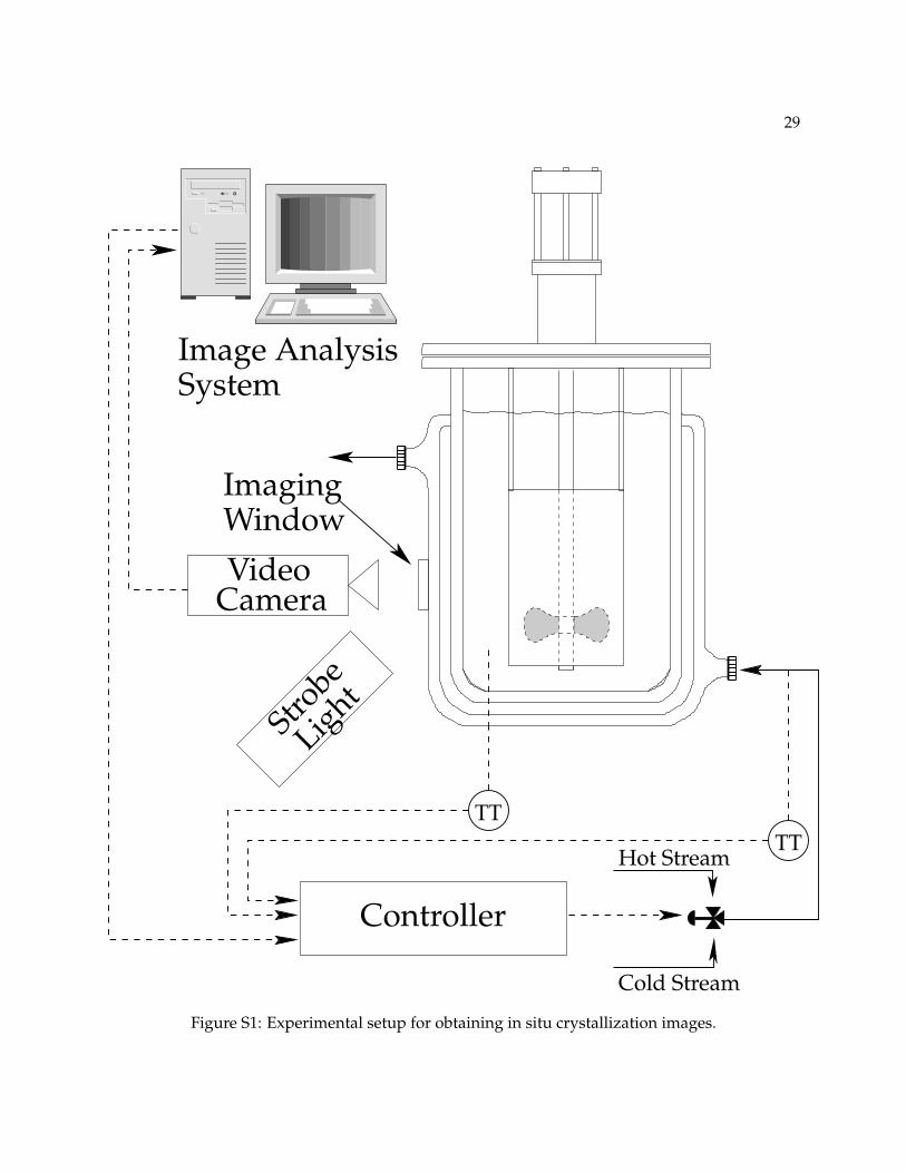
29

VideoCamera

ImagingWindow

Strobe

Light

Image AnalysisSystem

Controller

TTTT

Hot Stream

Cold Stream

Figure S1: Experimental setup for obtaining in situ crystallization images.

30

4.3 Data Acquisition and Control

4.3.1 Hardware

4.3.2 Software

4.3.3 Temperature control

4.4 Chemical Systems

4.4.1 Industrial pharmaceutical

4.4.2 Glycine

31

Chapter 5

Two-dimensional Object Recognition forHigh-Aspect-Ratio ParticlesSuspension crystallization processes often result in crystals having a high aspect ratio, a shapecommonly described as needle-like, rod-like, or acicular. High-aspect-ratio crystals are particu-larly commonplace in the specialty chemical and pharmaceutical industries as these industries de-velop complex, high-value-added chemical compounds. Controlling the particle size distribution(PSD) during crystallization of these compounds is critical, both to the efficiency of the down-stream manufacturing processes and to the quality of the end-product. However, conventionalPSD monitoring technologies, such as laser diffraction and laser backscattering, do not provide themonitoring capability necessary to achieve on-line PSD control for systems in which the particlesare highly non-spherical [15]. Laser diffraction overestimates the broadness of the spherical diam-eter distribution for high-aspect-ratio particles due to orientation effects and the spherical modelsused to interpret the diffraction data [119, 77]. The chord length distribution measured using laserbackscattering can be inverted theoretically to obtain the PSD for high-aspect-ratio particles, butthe inversion is highly ill-posed [116] and requires assumptions regarding the particle shape. Suc-cessful inversion has been demonstrated experimentally for spheres [50] and octahedra [116], buthas been demonstrated for high-aspect-ratio particles using simulations only [63].

Imaging offers the potential to extract both size and shape information and is thereforea promising and attractive approach for obtaining PSD’s for non-spherical particles. Several re-searchers have developed imaging-based methods for sizing elongated crystals [88, 96, 82, 83], butnone of these methods are sufficiently automated to be suitable for on-line monitoring and con-trol. Several commercial, imaging-based, on-line particle size and shape analyzers have recentlybecome available, such as Malvern’s Sysmex FPIA 3000 and Beckman-Coulter’s RapidVUE (see[3] for a survey of other imaging-based instruments). Most of these instruments require sampling,however, which is inconvenient, possibly hazardous, and raises concerns about whether the sam-ple is representative of the bulk slurry [3, 7].One exception is the Mettler Toledo Lasentec ParticleVision and Measurement (PVM) in situ probe. This probe is packaged with automatic image anal-ysis software that, although useful for some systems, does not give suitable results for systems ofneedle-like particles. The utility of in situ video microscopy has been limited primarily to quali-tative monitoring because the nature of in situ images, which contain blurred, out-of-focus, andoverlapping particles, has precluded the successful application of image analysis to automaticallyquantify particle size and shape [15].

The main barrier to successful automation of image analysis for in situ images is “segmen-

32

tation,” that is, separating the objects of interest from the background. Segmentation is simpli-fied if particles are imaged using transmitted light because the particle outlines are easily distin-guished [86]. To handle high solids concentrations, however, in situ imaging is constrained touse reflected light, so segmentation is more difficult. [19] presented a technique for automaticsegmentation of in-process suspension crystallizer images, but the technique was demonstratedonly on images that appear to have been acquired at low solids concentration where there are nooverlapping particles and the particles’ edges are well-defined. [55] used an in situ fluorescenceimaging method that caused the liquid phase of a fluidized bed to fluoresce while leaving the coalparticles opaque, thus enabling a gray-level theshold method to detect particle edges. However,for dense particle volume fractions, manual intervention was required to determine which of thesegmented particles could be used for sizing.

The goal of this work is to demonstrate robust and efficient segmentation for in situ imagesof high-aspect-ratio particles using a novel image analysis algorithm. To achieve this goal, weshow that the algorithm’s PSD measurements are consistent with measurements obtained throughmanual image analysis by human operators. The accuracy of the measured PSD, therefore, isestablished only with respect to the PSD measured by human operators. The absolute accuracyof the measured PSD depends on several factors, including the focal depth, the field of view, thesolids concentration, the PSD, the particle aspect ratio, and the hydrodynamics of the imagedvolume. A complete description of the effects of all of these factors on the absolute accuracy of themeasured PSD is beyond the scope of this paper but is a topic of current research in our laboratory.

The chapter is organized as follows. Section 6.2 describes the algorithm, and Section 5.2presents the experimental studies used to evaluate the algorithm’s accuracy and speed. Our find-ings are summarized in Section 8.6.

5.1 Image Analysis Algorithm Description

This section describes the image analysis algorithm developed for the purpose of analyzing insitu images of high-aspect-ratio crystals. The algorithm is referred to in this paper as SHARC(Segmentation for High-Aspect-Ratio Crystals) and has been implemented in MATLAB 7.1. Wepresent first an overview of SHARC and then describe in more detail each of SHARC’s compo-nents.

5.1.1 Overview

The SHARC algorithm is built on the assumption that a needle-shaped crystal can be modeledgeometrically as a group of two or more spatially-proximate lines with similar orientation andlength. The SHARC algorithm searches for image features satisfying this model in the follow-ing manner: First, SHARC detects linear features in the image, referred to as “elementary linesegments” or ELSs. Next, SHARC identifies collinear line pairs (lines that appear to belong to asingle crystal edge but have been broken up due to background noise, particle overlap, or crys-tal defects) and creates a representative line, called a “base line,” for each pair. Given both the

33

ELSs and the base lines, SHARC identifies pairs of spatially-proximate, parallel lines of similarlength. Finally, SHARC identifies consistent groups of parallel lines and clusters the constituentlines in each of these groups as belonging to a single crystal. The properties (e.g. length, aspectratio) of these line clusters are used as estimates of the properties of the crystals in the image. Fig-ure S1 shows the result of applying these steps to a small section of an in situ image of needle-likepharmaceutical crystals.

5.1.2 Linear Feature Detection.

Line segments are commonly used as inputs to higher-level processes in machine vision, andmany different methods have been developed for extracting line segments from images (see [53]for a review of these methods). SHARC uses the Burns line finder [17]. For our application, theBurns line finder is advantageous over the popular Hough transform-based methods for severalreasons. First, the Burns line finder is scale-independent, that is, it finds short lines just as easilyas it finds long lines. The Burns line finder also has lower computation and memory requirementsthan the Hough transform and finds line endpoints more easily. The Burns line finder is uniquein that it detects lines on the basis of image intensity gradient direction, whereas most line-findersare based on image intensity gradient magnitude. The Burns line finder is therefore able to detectsubtle linear features that would be missed by other line finders. This feature also means thatits performance is relatively insensitive to variations in contrast and brightness. This propertyis important for crystallization imaging because, as crystallization occurs, the increasing solidsconcentration causes more reflected light to reach the camera CCD, resulting in image intensityvariations. Such variations do not affect the performance of the Burns line finder.

We have modified slightly the Burns algorithm to enhance its performance for our partic-ular application, incorporating some of the speed-up suggestions given by [54]. Our implementa-tion consists of the following steps:

1. Calculate the direction and magnitude of the image intensity gradient at each pixel using aSobel gradient operator of size n∇ × n∇.

2. For each pixel with gradient magnitude above a small threshold ε|∇|, assign a gradient direc-tion label by coarsely quantizing the pixel’s gradient direction into one of nb sets of ranges,or “buckets,” as depicted in Figure S2.

3. Apply a connected components algorithm (CCA) to group identically-labeled, adjacent (in-cluding diagonally adjacent) pixels into “line support regions,” as depicted in Figure S3.

4. Filter line support regions that have a pixel area less than some pre-defined threshold εA.

5. Fit a line to each remaining line support region, as depicted in Figure S3.

To eliminate quantization effects, steps 2–4 are performed twice before proceeding to step5, each time using a different quantization in which the gradient direction partitioning is shifted byhalf the bucket size, as shown in Figure S2. This procedure results in each pixel being associated

34

(a) (b)

(c) (d)

Figure S1: Example of SHARC algorithm applied to an in situ image of suspended pharmaceuticalcrystals. (a) A region of interest in the original image. (b) Linear features (ELSs) extracted from theoriginal image. (c) ELSs (black lines) and lines representing each collinear line pair (white lines).(d) Representative rectangles for clusters of spatially-proximate parallel lines with roughly equallength. The lengths, widths, and aspect ratios of the rectangles are used as the crystal size andshape measurements.

with two different line support regions, and this conflict is resolved through a voting processdesigned to select the interpretation that results in the longest possible line support regions [17].To reduce computation time, SHARC carries out this voting process on the basis of the pixel areasof the conflicting line support regions, which in almost every case gives the same results as voting

35

23

14

5

6 7

81

23

4

5

67

8

Figure S2: Depiction of different eight-bucket gradient direction quantizations used to label pixels.For the quantization on the left, pixels having gradient direction in the range of 0 to 45 degrees arelabeled as “1”, pixels with gradient direction in the range of 45 to 90 degrees are labeled as “2”,and so forth. Quantization effects are mitigated by applying a second quantization, such as thatshown on the right, and subsequently resolving any conflicts between the results given by eachquantization.

based on length.The line-fitting method used in step 5 is standard blob analysis, available in most image

analysis packages. Blob analysis fits a line to each region of pixels by determining an ellipsehaving the same geometric moments as the region, as depicted in Figure S3. The ellipse’s majoraxis length, minor axis length, orientation, and centroid are used respectively as the length, width,orientation, and center of the corresponding line.

5.1.3 Identification of Collinear Line Pairs

During linear feature extraction, single edges are commonly broken up into multiple collinearlines. This problem is common for systems of needle-like crystals because the particles are of-ten touching or overlapping. Therefore, SHARC groups these collinear lines prior to searchingfor groups of parallel lines having similar length and orientation. The problem of collinear linegrouping has been studied extensively. [53] compare and evaluate a number of the availablemethods. SHARC uses a straightforward, computationally inexpensive method developed by[31]. Etemadi’s method involves projecting ELSs of similar orientation onto a common line todetermine if the lines satisfy simple spatial-proximity thresholds given by

|θ1 − θ2| < εθC, dPD < εPD(w1 + w2), dEP < εEP(LP

1 + LP2 ) (5.1)

in which dPD is the perpendicular distance between the two lines and dEP is the distance betweentheir nearest projected endpoints. θi and wi are, respectively, the orientation and width of linei calculated using blob analysis, and LP

i is the projected length of line i, calculated as describedbelow. εθC

, εPD, and εEP are user-specified thresholds.The perpendicular and endpoint distances and projected lengths are calculated, as depicted

in Figure S4, by projecting the two lines onto a “virtual line” whose position (xV , yV ) and orien-tation (θV ) are length-weighted averages of the positions and orientations of the constituent ELSs,

36

(a) (b)

(c) (d)

Figure S3: Example of finding linear features using Burns line finder and blob analysis. (a)Grayscale image. (b) Regions of pixels having similar gradient orientation, determined using theBurns line finder. (c) Best-fit ellipses for each region of pixels, determined using blob analysis. (d)Major axes of the best-fit ellipses imposed on the original grayscale image.

given by

xV =L1x1 + L2x2

L1 + L2, yV =

L1y1 + L2y2

L1 + L2, θV =

L1θ1 + L2θ2

L1 + L2(5.2)

in which Li, θi, xi, and yi are the length, orientation, horizontal centroid, and vertical centroid ofELS i, calculated using blob analysis. Given the position and orientation of the virtual line, theperpendicular distance between the two ELSs can be calculated as the sum of the perpendiculardistances of the ELSs centroids from the virtual line. The length of the virtual line, LV , is definedas the length of the shortest possible line containing all four projected endpoints.

For each line pair satisfying the collinearity criteria, the corresponding virtual line becomesa base line and is subsequently used in the identification of parallel pairs, as described in thefollowing section.

37

P4

P3

dPD

y

x

Line 2

Line 1

θ1

(x2, y2)(x1, y1)

dPD1

dPD2

θ2

dEP

Virtual Line

P2

LP2

LP1

θV

P1

(xV , yV )

Figure S4: Depiction of variables used in line pair classification scheme.

5.1.4 Identification of Parallel Line Pairs

Following collinear line pair identification, SHARC identifies pairs of parallel lines, or lines thathave similar orientation, are spatially proximate, and exhibit a high degree of overlap when pro-jected onto a common line. These line pairs satisfy the following criteria:

|θ1 − θ2| < εθP, dPD <

1εAR

Lmax, QP > εQ (5.3)

in which εθP, εAR, and εQ are user-specified thresholds for orientation difference, aspect ratio, and

pair “quality.” dPD is the perpendicular distance between the two lines, and LV is the length ofthe virtual line, as defined in the previous section. Lmax is the length of the longest line in the pair,and QP quantifies the “quality” of the pair. The quality metric used by SHARC, and suggestedby [31], is based on the degree of overlap of the two parallel lines, calculated using

QP =LP

1 + LP2

2LV(5.4)

in which the projected lengths LPi are computed as described in Section 5.1.3. This metric is simple

to compute and scale-independent, depending only on the relative lengths of the lines. Overlap-ping parallel pairs give a QP between 0.5 and 1, the latter value representing a perfectly overlap-ping pair.

If the parallel pair includes a base line comprising two collinear ELSs, it is possible thatthe two lines in the parallel pair share an ELS, in which case the pair is invalid and is discarded.Figure S5 depicts examples of valid and invalid parallel pairs.

Each parallel pair is ranked according to its significance, calculated as

S =L2

min

Lmax(5.5)

38

1

2

3

45

62

1

34

52

13

(a) (b) (c)

Figure S5: Examples of valid and invalid parallel line pairs. The solid lines represent ELSs and thedotted lines represent base lines (lines arising from instances of collinearity). In (a), the base lines5 and 6 form a valid parallel pair, and the ELSs 3 and 4 also form a valid parallel pair. In (b), theparallel lines 4 and 5 are an invalid parallel pair because they both depend upon ELS 3. Similarly,in (c), base line 3 and ELS 1 form an invalid pair because both depend on ELS 1.

in which S is the significance level and Lmin and Lmax are, respectively, the lengths of the shorterand longer lines in the pair. This significance measure is used to account for the fact that longerlines are less likely to have arisen by accident or due to noise and should thus be considered moresignificant. The significance ranking is used to order the subsequent line clustering procedurebut affects the results only when there is a conflict between two high quality pairs, or when twohigh quality pairs are mutually exclusive. These conflicts arise since SHARC identifies parallelpairs using both the ELSs and the base lines (for example, ELSs 3 and 4 in Figure S5(a) form avalid parallel pair but are also involved indirectly in the parallel pair of base lines 5 and 6). If agiven ELS is involved in two conflicting parallel pairs, the significance ranking is used in the lineclustering process to favor the interpretation that leads to the longer crystal.

5.1.5 Clustering

The objective of clustering is to group those lines that appear to belong to a single crystal. The clus-ters are formed by (1) identifying the most significant parallel pair on the basis of equation (5.5),(2) recursively identifying all other lines that are parallel-paired with at least one of the lines inthe current cluster, and (3) removing from the list of parallel pairs any pairs that include an ELSor base line associated with the newly-formed group. This process is iterated until the list of par-allel pairs is empty, after which all lines that are not included in any of the formed groups arediscarded.

The properties of each line cluster are calculated using the method described in Section 5.1.3,generalized to an arbitrary number of lines. That is, the cluster orientation is the length-weightedaverage of all lines in the cluster, the cluster length is the length of the shortest possible line con-taining all projected endpoints for all lines in the cluster, and the cluster width is the largest pos-sible perpendicular distance between the centroids of all lines in the cluster. Clusters having anaspect ratio below the user-defined threshold εAR are discarded.

39

(a) (b)

(c) (d)

Figure S6: Example of clustering procedure for valid parallel pairs. (a) ELSs (dark) and base lines(light) involved in at least one valid parallel pair. (b) The pair with the highest significance. (c)Lines that are parallel-paired (either directly or indirectly) with either of the lines in the highestsignificance pair. (d) The bounding box calculated for the line cluster.

Figure S6 illustrates the clustering procedure using the set of lines extracted in Figure S3.Figure S6(a) shows all lines involved in at least one valid parallel pair, including both ELSs andbase lines. The valid parallel pairs for this example are (10,14), (12,15), (18,19), (18,20), and (19,21).Lines 18, 19, 20, and 21 are base lines comprising the collinear pairs (9,15),(10,12),(12,14), and(14,15), respectively. Figure S6(b) shows that pair (18,20) has the highest significance and is there-fore analyzed first in the clustering order. Figure S6(c) shows the result of recursively identifyingall lines that are paired with lines in the cluster. That is, line 19 is identified in the first recursiondue to its pairing with line 18, and line 21 is identified in the second recursion due to its pair-ing with line 19. The rectangle in Figure S6(d) indicates the length, width, and orientation of theline cluster. The parallel pairs (10,14) and (12,15), each of which has at least one of its membersinvolved in the newly-formed grouping, are removed from the list of parallel pairs.

40

15

20

25

30

35

40

45

50

55

0 50 100 150 200 250 300

Tem

pera

ture

,[

C]

Time, [minutes]

t1 t2 t3 t4 t5 t6

Seeds injected

Figure S7: Temperature trajectory for crystallization experiment. The vertical lines indicate thetimes at which sets of video images were acquired.

Line finder Collinearity ParallelismParameters Thresholds Thresholds

n∇ 5 εθC20 degrees εθP

5 degreesε|∇| 1 εEP 0.5 εQ 0.85nb 6 buckets εPD 0.5 εAR 4.5εA 20 pixels

Table 5.1: Parameter values used to analyze images from crystallization experiment.

5.2 Experimental Results

To evaluate SHARC’s performance, a seeded, pharmaceutical crystallization was carried out dur-ing which several sets of video images were acquired. The images in each set were acquired overa few seconds only, such that we assume the properties of the crystal population are constant foreach image set. The temperature profile (following seed injection) for this crystallization is shownin Figure S7. The time at which each set of video images was acquired is indicated in Figure S7 bya vertical line and labeled as tj , the subscript indicating the image set number. The mixing speedfor this experiment was 550 RPM (1.1 m/s tip speed), sufficiently fast that the crystals could notbe tracked from one video frame to the next. The same parameter values were used to analyze allimages (see Table 8.2).

The following sections assess SHARC’s suitability for on-line monitoring and control withrespect to both accuracy and speed.

41

5.2.1 Algorithm Accuracy

Visual Evaluation

Figures S8–S11 show SHARC’s performance on selected images taken from video sets 3, 4, 5, and6. These figures demonstrate SHARC’s effectiveness for images having poor contrast and un-even background. These figures also demonstrate SHARC’s ability to detect crystals with poorly-defined edges, varying intensity levels, and a certain level of particle overlap.

Comparisons with Manual Sizing

We evaluate SHARC’s accuracy by comparing its PSD measurements with measurements ob-tained through manual image analysis by human operators. Although the human vision systemis clearly more reliable than current computer vision systems, manual image analysis introducesan undesirable level of subjectiveness into the measurement. The subjectiveness of manual sizingis magnified for in situ images because the crystals often appear blurry, overlapping, and out-of-focus. Thus, it can be difficult to decide whether or not a given crystal is sufficiently in focus andwell-defined to be sized accurately. To assess the subjectiveness involved in manually sizing insitu images and determine what constitutes “good” agreement between SHARC’s measurementand a manual measurement, we asked nine different people to manually size crystals for the sameten images from image set 3. We confirmed that ten images was sufficient to achieve convergenceof the overall mean size measurement for each operator. Table ?? shows the overall mean sizecalculated for all ten images for each operator, the total number of crystals found by each opera-tor, and the average percent difference in overall mean size between each operator and the otheroperators. This latter value is calculated for operator i using the equation

diffi =100

Nop − 1

Nop∑j=1

|xi − xj |xi+xj

2

(5.6)

Table ?? shows that the mean size varied by as much as 37% between operators, and the numberof crystals found varied by over 100% between operators, illustrating the large degree of subjec-tiveness associated with manual sizing of in situ images. However, the relatively small standarddeviation in overall mean size indicates that manual sizing constitutes a reasonably reliable stan-dard provided the measurement is performed by a sufficient number of operators.

Based on the results shown in Table ??, we define “good” agreement between SHARC’sresults and a set of manual results to mean that their individual means are within approximately12% of their combined mean value. Table 5.2.1 shows that the SHARC algorithm determines amean crystal size within 2% of that found by the nine manual operators, and Figure S12 shows agood match between the cumulative distribution function found by SHARC and the cumulativedistribution functions of the nine manual operators.

To evaluate SHARC’s ability to maintain accuracy for the duration of the experiment,twenty-five images from sets 4, 5, and 6 were analyzed both manually (by a single operator)and using SHARC. Table 5.2.1 shows that SHARC maintains good agreement with the results

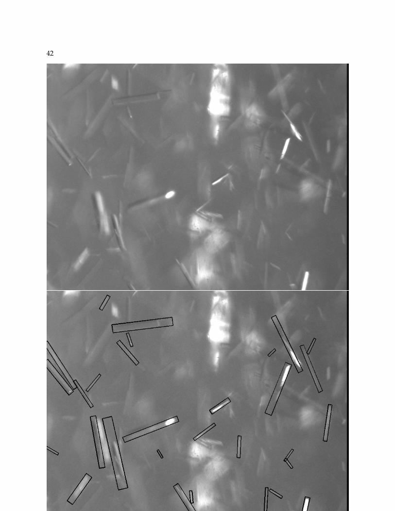
42

Figure S8: Algorithm performance on example image (set 3, frame 1).

43


44


45


46

Mean Size, [µm]Image set Manual Automatic % Difference

3 283 284 0.34 290 286 1.25 306 278 9.36 355 283 22.5

Table 5.2: Comparison of mean sizes calculated from manual sizing of crystals and from automaticsizing.

0

0.2

0.4

0.6

0.8

1

0 200 400 600 800 1000

Cum

ulat

ive

num

ber

frac

tion

Size, [µm]

SHARCManual

0

0.2

0.4

0.6

0.8

1

0 200 400 600 800 1000

Cum

ulat

ive

num

ber

frac

tion

Size, [µm]

SHARCManual

Set 3 Set 4

0

0.2

0.4

0.6

0.8

1

0 200 400 600 800 1000

Cum

ulat

ive

num

ber

frac

tion

Size, [µm]

SHARCManual

0

0.2

0.4

0.6

0.8

1

0 200 400 600 800 1000

Cum

ulat

ive

num

ber

frac

tion

Size, [µm]

SHARCManual

Set 5 Set 6

Figure S12: Comparison of cumulative number fractions obtained from manual and automaticsizing of crystals for video image sets 3, 4, 5, and 6. Set 3 was manually sized by nine differentoperators.

obtained manually for sets 4 and 5, but its performance declines somewhat for set 6. These sameconclusions can be drawn from Figure S12, which compares the cumulative distribution functionsobtained using both methods.

Figure S12 and Table 5.2.1 indicate that, as the solids concentration and degree of crystalattrition increase, SHARC either fails to identify a significant percentage of the larger crystalsor erroneously identifies smaller crystals. Figure S13 shows the results of manually sizing an

47

2

14

5

610

15

12

3

79

8

13

14

11

Figure S13: Comparison of crystals sized manually (top) and using SHARC (bottom).

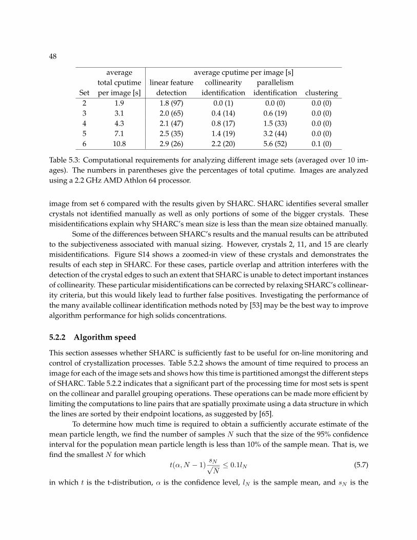
48

average average cputime per image [s]total cputime linear feature collinearity parallelism

Set per image [s] detection identification identification clustering2 1.9 1.8 (97) 0.0 (1) 0.0 (0) 0.0 (0)3 3.1 2.0 (65) 0.4 (14) 0.6 (19) 0.0 (0)4 4.3 2.1 (47) 0.8 (17) 1.5 (33) 0.0 (0)5 7.1 2.5 (35) 1.4 (19) 3.2 (44) 0.0 (0)6 10.8 2.9 (26) 2.2 (20) 5.6 (52) 0.1 (0)

Table 5.3: Computational requirements for analyzing different image sets (averaged over 10 im-ages). The numbers in parentheses give the percentages of total cputime. Images are analyzedusing a 2.2 GHz AMD Athlon 64 processor.

image from set 6 compared with the results given by SHARC. SHARC identifies several smallercrystals not identified manually as well as only portions of some of the bigger crystals. Thesemisidentifications explain why SHARC’s mean size is less than the mean size obtained manually.

Some of the differences between SHARC’s results and the manual results can be attributedto the subjectiveness associated with manual sizing. However, crystals 2, 11, and 15 are clearlymisidentifications. Figure S14 shows a zoomed-in view of these crystals and demonstrates theresults of each step in SHARC. For these cases, particle overlap and attrition interferes with thedetection of the crystal edges to such an extent that SHARC is unable to detect important instancesof collinearity. These particular misidentifications can be corrected by relaxing SHARC’s collinear-ity criteria, but this would likely lead to further false positives. Investigating the performance ofthe many available collinear identification methods noted by [53] may be the best way to improvealgorithm performance for high solids concentrations.

5.2.2 Algorithm speed

This section assesses whether SHARC is sufficiently fast to be useful for on-line monitoring andcontrol of crystallization processes. Table 5.2.2 shows the amount of time required to process animage for each of the image sets and shows how this time is partitioned amongst the different stepsof SHARC. Table 5.2.2 indicates that a significant part of the processing time for most sets is spenton the collinear and parallel grouping operations. These operations can be made more efficient bylimiting the computations to line pairs that are spatially proximate using a data structure in whichthe lines are sorted by their endpoint locations, as suggested by [65].

To determine how much time is required to obtain a sufficiently accurate estimate of themean particle length, we find the number of samples N such that the size of the 95% confidenceinterval for the population mean particle length is less than 10% of the sample mean. That is, wefind the smallest N for which

t(α, N − 1)sN√N≤ 0.1lN (5.7)

in which t is the t-distribution, α is the confidence level, lN is the sample mean, and sN is the

49

(a) (b) (c) (d)

Figure S14: Zoomed-in view of crystals that SHARC failed to identify correctly. From top tobottom, the crystal labels are two, eleven, and fifteen (according to labels in Figure S13). Column(a): Original image. Column (b): ELS data. Column (c): ELSs and base lines. Column (d): Resultof clustering.

50

average # of crystals cputime to cputime to# of crystals to converge converge to converge to

Set per image to mean mean [min.] variance [min.]2 1 93 1.9 18.53 25 163 0.3 1.84 28 129 0.3 2.25 30 106 0.4 3.46 38 143 0.7 4.2

Table 5.4: Computational requirements to achieve convergence of mean and variance.

sample standard deviation, defined as

lN =1N

N∑i=1

li (5.8)

sN =

√√√√ 1N − 1

N∑i=1

(li − lN )2 (5.9)

in which li is the length of particle i. Similarly, to determine how much time is required to obtaina sufficiently accurate estimate of the variance in particle length, we find N such that the size ofthe 95% confidence interval for the population variance is less than 10% of the sample variances2N , satisfying

N − 1χ2(α, N − 1)

− 1 ≤ 0.1 (5.10)

in which χ2 is the chi-squared distribution (see [101, p.75]). Equation 5.10 is satisfied for N = 889samples.

Given SHARC’s speed, the number of crystals per image, and the number of samples nec-essary to obtain sufficient measurement accuracy, we can calculate the rate at which SHARCprovides accurate mean and variance measurements. Table 5.4 indicates that SHARC requiresapproximately two minutes to measure the PSD mean and fifteen minutes to measure the PSDvariance. Given the time scales of most crystallization processes, SHARC is sufficiently fast toprovide measurements for a feedback control system based on measurements of the PSD meanand variance. If necessary, the measurement rate can be increased by implementing SHARC in acompiled language.

5.3 Conclusion

The SHARC algorithm can robustly and efficiently extract crystal size information from in situimages of suspended, high-aspect-ratio crystals for moderate solids concentrations, giving re-sults consistent with measurements obtained through manual image analysis by human opera-tors. SHARC’s performance declines for high solids concentrations and high levels of particle

51

attrition because the degree of particle overlap and the noise arising from attrited particulate mat-ter hinder the identification of the suspended crystals’ edges. Implementing improved methodsfor identifying instances of collinearity may enable suitable performance for these conditions.

The speed with which SHARC analyzes the images is suitable for real-time monitoring andcontrol of PSD mean and variance.

We gratefully acknowledge GlaxoSmithKline for providing the imaging system used inthis study. We also gratefully acknowledge the financial support of the industrial members of theTexas-Wisconsin Modeling and Control Consortium. Finally, we wish to thank Joshua, Jeremiah,and Mary Diaz, Aaron Lowe, Murali Rajamani, Ethan Mastny, Michael Benton, and ThomasKnotts, who willingly performed tedious manual sizing of the imaged crystals.

52

Chapter 6

Three-dimensional Object Recognitionfor Complex Crystal ShapesSolution crystallization processes are widely used in the pharmaceutical, food, and chemical in-dustries to create solids with desirable properties and separate or purify chemical species. Con-trolling the particle size distribution (PSD) and the distribution of particle shapes during crystal-lization is critical, both to the efficiency of the downstream manufacturing processes and to thequality of the end-product. However, conventional PSD monitoring technologies, such as laserdiffraction and laser backscattering, are based on assumptions of particle sphericity and thus donot provide the monitoring capability necessary to achieve on-line PSD control for systems inwhich the particles are highly non-spherical [119, 15]. Although methods have been developedfor inverting the chord length distribution (CLD) measured by laser backscattering to estimate thePSD [94, 116, 63], successful application of these methods has been demonstrated experimentallyonly for spheres [50] and octahedra [116]. Furthermore, it has been shown that the CLD inversionfor high-aspect-ratio particles is highly ill-posed [116]. Finally, laser backscattering cannot mea-sure the shape of individual particles and therefore cannot measure the distribution of particlesbetween different shape classes (e.g. number of needles relative to number of spheres) nor shapefactor distributions (e.g. distribution of aspect ratios).

The limitations inherent in laser-scattering-based monitoring technologies motivate the useof imaging-based methods, which allow direct visualization of particle size and shape. Obtainingquantitative information from imaging-based methods, however, requires image segmentation.Image segmentation means separating the objects of interest (e.g. the particles) from the back-ground. Most commercial, imaging-based, on-line particle size and shape analyzers solve thesegmentation problem by imaging the particulate slurry as it passes through a specially-designedflow cell under controlled lighting conditions [3, p. 167]. The images acquired in this way can besegmented using simple thresholding methods. The drawback is that this approach requires sam-pling, which is inconvenient, possibly hazardous, and raises concerns about whether the sampleis representative of the bulk slurry. Alternatively, the images can be acquired in situ. Robust andefficient segmentation of in situ images is challenging, however, for several reasons. First, in situimaging typically requires illumination by reflected light in order to handle high solids concen-trations. Thus, the particles appear in the image with non-uniform color and intensity such thatthresholding methods are ineffective. The use of reflected light can also result in poorly-definedparticle outlines, thus limiting the robustness of methods based on closing the particle outlines,such as the technique proposed by [19]. Second, the crystals can have a large variation in size and

53

are randomly-oriented in 3-D space, which means the projections of the crystals onto the imagingplane can take on a wide variety of shapes. Hough-transform-based methods [41, p. 587], whichhave been applied extensively to segment images of circular or elliptical particles and droplets,involve exhaustive searches over the particle location and shape parameter space and are there-fore computationally infeasible for randomly-oriented particles of complex shapes. The imagesegmentation problem is further complicated by particle agglomeration, overlap, breakage, andattrition, which result in occluded or poorly-defined particle boundaries.

Model-based object recognition is a widely-used approach to computer vision that has beendeveloped to enable automatic recognition of complex objects with unknown pose (i.e. orientationwith respect to the camera) in the presence of missing or occluded data [51, 65, 37, chapter 18]. Themodel-based object recognition approach is based on matching raw image features (such as arcsor lines) with one of several pre-defined models. The model-based approach does not involveexhaustive searches of the model parameter space and is therefore more efficient than purely top-down approaches (such as Hough-transform-based methods). Model-based object recognition ismore robust to noise than purely bottom-up approaches because it can be applied even if part ofthe object to be identified is occluded or missing. Furthermore, the model-based approach leads toalgorithms that can be implemented in a parallel fashion to enable real-time analysis. Algorithmsbased on this approach have been developed and applied to systems of circular particles [99],elliptical particles [47], and rectangular or needle-like particles [59].

This paper describes a model-based object recognition algorithm that can be applied to im-ages of crystals of any shape, provided the shape can be represented as a wire-frame model. Thewire-frame models used by the algorithm are parameterized. Thus, a single model can be usedto identify crystal objects exhibiting a wide range of sizes and shapes within a given shape class.The algorithm therefore enables the measurement of shape factor distributions. Furthermore, thealgorithm can be applied using multiple wire-frame models representing different shape classesto measure the distribution of particles between different shape classes. The algorithm’s effective-ness is demonstrated by comparing the algorithm results with those obtained by manual, humananalysis of in situ video images acquired at different solids concentrations during an α-glycinecooling crystallization experiment. The paper is organized as follows: Section 8.4 describes thecrystallization experiment. Section 6.2 describes the algorithm, and Section 8.5 discusses the algo-rithm’s accuracy and speed.

6.1 Experimental

The α-glycine crystallization was carried out by dissolving 180 g of glycine (p.a., Acros Organics)in 600 mL of deionized water at 55 C. The solution was cooled to 25 C at 5 C/hr. Sponta-neous nucleation was observed around 29 C. Three sets of video images were acquired duringthe course of the experiment, each set consisting of 100 images acquired at a rate of 30 frames persecond. Each set was acquired once a noticeable increase in the solids concentration had occurred.The first set of video images was acquired approximately 13 minutes after nucleation at low solidsconcentration with the draft tube in the middle of the crystallizer clearly visible. The second set

54

t

t

h

Y

X

Z

w

w

Figure S1: Wire-Frame glycine crystal model. The parameters for the model are the crystal bodyheight, h, the width, w, and the pyramid height, t.

of images was acquired approximately 24 minutes after nucleation at medium solids concentra-tion with the draft tube just barely visible. The final set of images was acquired 43 minutes afternucleation at high solids concentration with the draft tube completely obscured by the slurry. Thepolymorphic form of the observed crystals was confirmed using X-ray powder diffraction.

6.2 Model-based recognition algorithm

This section describes the model-based recognition algorithm designed to extract crystal size andshape information from in situ crystallization images. The algorithm is called M-SHARC (Model-based SHApe Recognition for Crystals) and has been implemented in MATLAB 7.0.

6.2.1 Preliminaries

The model-based object recognition framework involves matching a set of primitive features ex-tracted from an image (such as points, corners, or lines) to a pre-defined set of models. The prim-itive image features used by M-SHARC are lines, and the models are parameterized, wire-framemodels. Wire-frame models consist of a set of q vertices V = XK [pm]K=1...q and a set of r lines oredges E = EJJ=1...r. XK is a three-dimensional vector defined in a model-centered coordinatesystem as a function of the model internal parameters pm. EJ is a set of two labels pointing to thevertices in V that are connected by edge J . The model used in this study was designed to capturethe range of shapes exhibited by crystals of glycine, an amino acid of importance in the pharma-ceutical industry. The model, shown in Figure S1, has three internal parameters (pm = (h, w, t)),20 edges, and 10 vertices.

To fit the wire-frame model to the linear features in the image, the model must be pro-jected onto the image plane. This projection is computed by first applying rigid-body rotationsand translations to change each model point X from the model-centered coordinate frame to the

55

Zy

x

Zc

Optical axis

f

Yc

Xc

Image plane

Y

X

Figure S2: Depiction of the perspective projection of the glycine model onto the image plane. Forsimplicity, the image plane is displayed in front of the camera.

camera-centered coordinate frame:

Xc = RzRyRxX + T (6.1)

in which Rz, Ry, and Rx are rigid-body rotation matrices, which are functions of the in-planeorientation θz and the orientations in depth θy and θx, respectively. T = (tx, ty, tz) is a translationvector. Next, each model point is projected onto the image plane according to some imagingmodel. Under perspective projection, the transformation from a 3-D model point Xc = (Xc, Yc, Zc)to an image point x = (x, y) is given by

x =f

ZcXc, y =

f

ZcYc (6.2)

in which f is the focal length of the camera. Figure S2 depicts the perspective projection of theglycine model onto the image plane. M-SHARC uses the “weak perspective” imaging model,which accurately approximates perspective projection provided the depth of the imaged objects issmall relative to the distance of the objects from the camera. Under such imaging conditions, f/Zc

and tz can be assumed constant for all objects. In this work, we let f/Zc = 1 and tz = 0.The projection of the model onto the image plane is completed by determining the lines that

are visible for the given pose. Given a convex model, the visible model lines can be determined bycomputing an outward normal vector (in camera-centered coordinates) for each surface of the 3-Dmodel. The sign of the dot product of this normal vector with the camera’s optical axis determines

56

whether or not the surface is visible. The visible model lines are the lines that bound the visiblesurfaces.

The projection of the wire-frame model onto the image plane results in a set of projectedmodel lines EP = (MJ ,TJ , LJ)J=1...m in which MJ is a vector pointing from the origin of theimage coordinate system to the midpoint of the Jth model line, TJ is the unit tangent of the line,LJ is the length of the line, and m is the number of visible model lines. The set of data lines aredefined similarly as S = (mj , tj , lj)j=1...n, in which n is the number of lines detected by the linefinder.

M-SHARC follows the approach developed by [65, 66], consisting of three main steps: First,M-SHARC identifies linear features in the image. Second, M-SHARC identifies linear feature clus-ters that appear significant on the basis of viewpoint-independent relationships such as collinear-ity, parallelism, and end-point proximity. Third, M-SHARC fits a three-dimensional, wire-framemodel to each significant linear feature cluster. The following sections describe each of these steps.

6.2.2 Linear feature detection

The M-SHARC algorithm uses the line finder proposed by [17], incorporating some of the speed-up suggestions given by [54] (see [59] for details). The Burns line finder detects lines by identify-ing regions of pixels having similar image intensity gradient orientation. By detecting lines on thebasis of gradient orientation (as opposed to gradient magnitude), the Burns line finder’s perfor-mance is relatively insensitive to variations in contrast and brightness. This property is importantfor crystallization imaging because, as crystallization occurs, the increasing solids concentrationcauses more reflected light to reach the camera CCD, which increases the image brightness whiledecreasing the image contrast.

During linear feature extraction, single physical edges are commonly broken up into mul-tiple collinear lines due to particle overlap, noise, or poor lighting. A key component of the algo-rithm, therefore, is the grouping of these collinear lines prior to searching for viewpoint-invariantline groups. The M-SHARC algorithm uses the method developed by [31] because it is straightfor-ward to implement and relatively inexpensive computationally. The method uses simple thresh-olding on the angle, perpendicular distance, and endpoint distance between two lines to deter-mine whether or not the lines are collinear. If collinearity requirements are met, M-SHARC createsa new line based on the collinear pair but also retains the two original lines in case the instanceof collinearity is accidental. Therefore, subsequent grouping operations operate on both the linescreated from collinear grouping and all lines determined by the Burns line finder (whether or notthey are involved in a collinear group). Retaining the original lines involved in collinear groupsmakes M-SHARC’s performance less sensitive to the collinear grouping thresholds.

6.2.3 Perceptual grouping

Perceptual grouping refers to the task of organizing primitive objects, such as points or lines, intohigher-level, meaningful structures. These structures, or groups, are useful as visual cues for thelocation, size, and orientation of a given object in the image. Viewpoint-invariant groups (VIGs),

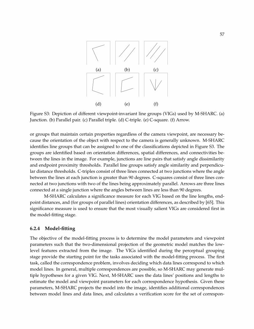
57

(a) (b) (c)

(d) (e) (f)

Figure S3: Depiction of different viewpoint-invariant line groups (VIGs) used by M-SHARC. (a)Junction. (b) Parallel pair. (c) Parallel triple. (d) C-triple. (e) C-square. (f) Arrow.

or groups that maintain certain properties regardless of the camera viewpoint, are necessary be-cause the orientation of the object with respect to the camera is generally unknown. M-SHARCidentifies line groups that can be assigned to one of the classifications depicted in Figure S3. Thegroups are identified based on orientation differences, spatial differences, and connectivities be-tween the lines in the image. For example, junctions are line pairs that satisfy angle dissimilarityand endpoint proximity thresholds. Parallel line groups satisfy angle similarity and perpendicu-lar distance thresholds. C-triples consist of three lines connected at two junctions where the anglebetween the lines at each junction is greater than 90 degrees. C-squares consist of three lines con-nected at two junctions with two of the lines being approximately parallel. Arrows are three linesconnected at a single junction where the angles between lines are less than 90 degrees.

M-SHARC calculates a significance measure for each VIG based on the line lengths, end-point distances, and (for groups of parallel lines) orientation differences, as described by [65]. Thissignificance measure is used to ensure that the most visually salient VIGs are considered first inthe model-fitting stage.

6.2.4 Model-fitting

The objective of the model-fitting process is to determine the model parameters and viewpointparameters such that the two-dimensional projection of the geometric model matches the low-level features extracted from the image. The VIGs identified during the perceptual groupingstage provide the starting point for the tasks associated with the model-fitting process. The firsttask, called the correspondence problem, involves deciding which data lines correspond to whichmodel lines. In general, multiple correspondences are possible, so M-SHARC may generate mul-tiple hypotheses for a given VIG. Next, M-SHARC uses the data lines’ positions and lengths toestimate the model and viewpoint parameters for each correspondence hypothesis. Given theseparameters, M-SHARC projects the model into the image, identifies additional correspondencesbetween model lines and data lines, and calculates a verification score for the set of correspon-

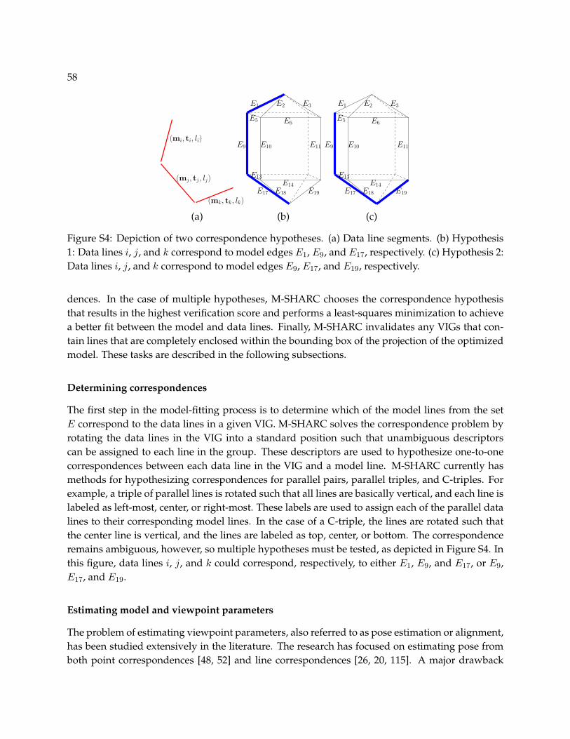
58

(mi, ti, li)

(mj, tj, lj)

(mk, tk, lk)

E11E10E9

E13E14

E19E18E17

E5 E6

E2 E3E1

E17 E18 E19

E14

E13

E9 E10 E11

E6E5

E1 E2 E3

(a) (b) (c)

Figure S4: Depiction of two correspondence hypotheses. (a) Data line segments. (b) Hypothesis1: Data lines i, j, and k correspond to model edges E1, E9, and E17, respectively. (c) Hypothesis 2:Data lines i, j, and k correspond to model edges E9, E17, and E19, respectively.

dences. In the case of multiple hypotheses, M-SHARC chooses the correspondence hypothesisthat results in the highest verification score and performs a least-squares minimization to achievea better fit between the model and data lines. Finally, M-SHARC invalidates any VIGs that con-tain lines that are completely enclosed within the bounding box of the projection of the optimizedmodel. These tasks are described in the following subsections.

Determining correspondences

The first step in the model-fitting process is to determine which of the model lines from the setE correspond to the data lines in a given VIG. M-SHARC solves the correspondence problem byrotating the data lines in the VIG into a standard position such that unambiguous descriptorscan be assigned to each line in the group. These descriptors are used to hypothesize one-to-onecorrespondences between each data line in the VIG and a model line. M-SHARC currently hasmethods for hypothesizing correspondences for parallel pairs, parallel triples, and C-triples. Forexample, a triple of parallel lines is rotated such that all lines are basically vertical, and each line islabeled as left-most, center, or right-most. These labels are used to assign each of the parallel datalines to their corresponding model lines. In the case of a C-triple, the lines are rotated such thatthe center line is vertical, and the lines are labeled as top, center, or bottom. The correspondenceremains ambiguous, however, so multiple hypotheses must be tested, as depicted in Figure S4. Inthis figure, data lines i, j, and k could correspond, respectively, to either E1, E9, and E17, or E9,E17, and E19.

Estimating model and viewpoint parameters

The problem of estimating viewpoint parameters, also referred to as pose estimation or alignment,has been studied extensively in the literature. The research has focused on estimating pose fromboth point correspondences [48, 52] and line correspondences [26, 20, 115]. A major drawback

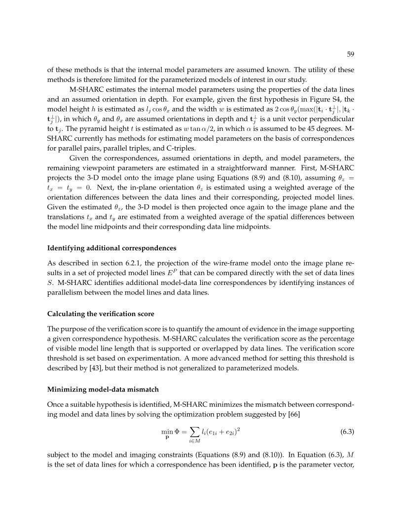
59

of these methods is that the internal model parameters are assumed known. The utility of thesemethods is therefore limited for the parameterized models of interest in our study.

M-SHARC estimates the internal model parameters using the properties of the data linesand an assumed orientation in depth. For example, given the first hypothesis in Figure S4, themodel height h is estimated as lj cos θx and the width w is estimated as 2 cos θy(max(|ti · t⊥j |, |tk ·t⊥j |), in which θy and θx are assumed orientations in depth and t⊥j is a unit vector perpendicularto tj . The pyramid height t is estimated as w tanα/2, in which α is assumed to be 45 degrees. M-SHARC currently has methods for estimating model parameters on the basis of correspondencesfor parallel pairs, parallel triples, and C-triples.

Given the correspondences, assumed orientations in depth, and model parameters, theremaining viewpoint parameters are estimated in a straightforward manner. First, M-SHARCprojects the 3-D model onto the image plane using Equations (8.9) and (8.10), assuming θz =tx = ty = 0. Next, the in-plane orientation θz is estimated using a weighted average of theorientation differences between the data lines and their corresponding, projected model lines.Given the estimated θz , the 3-D model is then projected once again to the image plane and thetranslations tx and ty are estimated from a weighted average of the spatial differences betweenthe model line midpoints and their corresponding data line midpoints.

Identifying additional correspondences

As described in section 6.2.1, the projection of the wire-frame model onto the image plane re-sults in a set of projected model lines EP that can be compared directly with the set of data linesS. M-SHARC identifies additional model-data line correspondences by identifying instances ofparallelism between the model lines and data lines.

Calculating the verification score

The purpose of the verification score is to quantify the amount of evidence in the image supportinga given correspondence hypothesis. M-SHARC calculates the verification score as the percentageof visible model line length that is supported or overlapped by data lines. The verification scorethreshold is set based on experimentation. A more advanced method for setting this threshold isdescribed by [43], but their method is not generalized to parameterized models.

Minimizing model-data mismatch

Once a suitable hypothesis is identified, M-SHARC minimizes the mismatch between correspond-ing model and data lines by solving the optimization problem suggested by [66]

minp

Φ =∑i∈M

li(e1i + e2i)2 (6.3)

subject to the model and imaging constraints (Equations (8.9) and (8.10)). In Equation (6.3), M

is the set of data lines for which a correspondence has been identified, p is the parameter vector,

60

Correspondingmodel line

li

Data line i

e1i

e2i

Figure S5: Depiction of variables used in mismatch calculation for a single line correspondence.

li is the length of data line i, and e1i and e2i are the perpendicular distances from data line i’sendpoints to the corresponding model line, as depicted in Figure S5. The parameter vector for theglycine model in Figure S1 is

p =[

h t w θx θy θz tx ty

](6.4)

Invalidating overlapping VIGs

The VIGs identified during M-SHARC’s perceptual grouping stage can overlap, sharing lines.We assume, however, that each line in the image can be attributed to only one crystal. Thus,once a model is successfully fit to a set of lines, any VIG that contains one or more of those linesis considered invalid. Furthermore, we assume that any line completely contained within thebounding box of an identified crystal has arisen due to unmodeled features of that crystal. Thus,any VIG that contains one or more of these lines is also considered invalid. M-SHARC does notattempt to fit a model to invalid VIGs.

Applying this constraint on overlapping VIGs is advantageous in that it significantly re-duces the number of VIGs investigated, thus increasing M-SHARC’s efficiency. Furthermore, ini-tial studies indicated that a large number of false positives are identified if VIG invalidation is notemployed. Thus, the overlapping crystal constraint serves to increase the algorithm’s accuracy aswell as reduce the computational burden such that the algorithm can run in real-time on a singleprocessor. However, this feature requires M-SHARC to investigate each VIG serially, starting withthe most significant VIG and proceeding to the least significant, such that M-SHARC currentlycannot be implemented in parallel.

6.2.5 Summary and example

The M-SHARC algorithm can be summarized using the following pseudo-code:

1. Detect linear features in image

2. Identify and sort viewpoint-invariant line groups (VIG)

For each VIG

If VIG is valid

61

(a) (b) (c) (d)

(e) (f) (g) (h)

Figure S6: Result of applying M-SHARC to image of α-glycine crystal. (a) Original region of inter-est. (b) Linear features extracted using Burns line finder (dark lines). (c) Linear features extractedusing collinear grouping (light lines). (d) Most salient line group. (e) Model initialization. (f)Identification of additional correspondences. (g) Optimized model fit. (h) Invalidated VIGs.

3. Generate correspondence hypotheses

For each hypothesis

4. Estimate model and viewpoint parameters

5. Project model into image

6. Search for additional correspondences

7. Compute verification score

Endfor

8. Select hypothesis with highest score

If (score > Verification threshold)

9. Minimize model-data mismatch

10. Save optimized model information

11. Invalidate overlapped VIGs

Endif

Endif

Endfor

Figure S6 shows the step-by-step results of applying the M-SHARC algorithm to a region ofinterest from an image of α-glycine crystals. This region of interest contains a large, well-definedcrystal that is partially overlapped by a small, poorly-defined crystal. Applying the line finder to

62

the image in Figure S6(a) produces the dark lines shown in Figure S6(b). Because of overlap by thesmaller crystal, a few of the edges of the larger crystal are broken up into two or more lines. Usingcollinear line grouping, these broken-up lines are combined into the single, light lines displayedin Figure S6(c). In the perceptual grouping stage, the line group that is identified as being mostsignificant is the triple of parallel lines shown in Figure S6(d). The lengths, spatial positions, andrelative distances between these lines provide the information necessary to estimate the internalmodel parameters and pose, resulting in the model projection shown in Figure S6(e). In this figure,the thin, solid lines are the visible model lines while the dashed lines are the non-visible modellines. Figure S6(f) shows the additional correspondences between model and data lines found byidentifying instances of parallelism between the visible model lines in Figure S6(e) and the datalines in Figure S6(c). Figure S6(g) shows the optimized model obtained by minimizing the per-pendicular distances between each of the model-data line correspondences. Finally Figure S6(h)indicates three of the VIGs that are invalidated due to overlap with the identified model.

6.3 Results

To assess our algorithm’s performance, we carried out an unseeded, α-glycine cooling crystalliza-tion. Following spontaneous nucleation, we acquired three sets of video images at varying solidsconcentrations with 100 images in each set. Given the rate of acquisition (30 frames per second),each set of images essentially represents a snapshot in time. All images were analyzed by M-SHARC using the same set of parameters. The VIGs used to initialize model-fitting were paralleltriples and C-triples.

6.3.1 Visual evaluation

Figures S7–S9 show the results of applying M-SHARC to images acquired at low, medium, andhigh solids concentrations. These figures demonstrate M-SHARC’s ability to identify crystals cov-ering a wide range of sizes and orientations. These figures also demonstrate M-SHARC’s abilityto handle poor image quality. Although several options exist for improving the images, such aslowering the mixing rate to decrease motion blur, successful image analysis of these low-qualityimages demonstrates M-SHARC’s robustness and helps ensure success in the rugged industrialenvironment.

6.3.2 Comparison with human analysis

To quantify M-SHARC’s performance, we compare its results with the results obtained by man-ual analysis of the images by human operators. All 300 images acquired during the α-glycinecrystallization were analyzed both by M-SHARC and by a human operator. The human operatorannotated the images using LabelMe, a database and web-based image annotation tool developedby [95]. The images and annotations are available to the general scientific community through theLabelMe website.

63

Figure S7: M-SHARC segmentation results for selected images acquired at low solids concentra-tion (13 min. after appearance of crystals).

Figure S10 illustrates how M-SHARC’s results are compared with the human operator’sresults. Figure S10(b) shows the crystal outlines determined by the human operator while Fig-ure S10(c) shows the outlines determined by M-SHARC. Each outline is simply a set of straightlines. If a sufficiently large set of correspondences can be found between the set of lines in an M-SHARC outline and the set of lines in a human outline, the crystal corresponding to those outlinesis classified as a hit. If a sufficiently large set of correspondences is not found between a givenM-SHARC outline and any other human outline, the crystal corresponding to the M-SHARC out-line is classified as a false positive. Similarly, a crystal identified by a human operator for which nocorresponding M-SHARC outline can be found is classified as a miss. In Figure S10(d), the falsepositives are displayed in white and the misses in black.

Table 6.1 shows the number of hits NH , misses NM , and false positives NFP identifiedby comparing M-SHARC’s results with the human operator’s results for each of the three sets ofvideo images, along with number and area fractions for the hits and false positives. The hit, miss,and false positive areas (AH , AM , and AFP , respectively) are calculated based on the areas of thepolygons defined by each crystal outline. For each level of solids concentration, the hit numberfraction is significantly less than the hit area fraction while the false positive number fraction iscomparable to the false positive area fraction. Thus, we would expect the number-based area dis-tribution to be biased towards larger particles. This expectation is verified by Figure S11, whichcompares the number-based cumulative distribution functions (CDFs) for particle area. As a stan-dard of comparison, Figure S11 also shows the CDFs constructed using only particles classifiedas hits. The confidence interval displayed in these figures is calculated using the Kolmogorov-

64

Figure S8: M-SHARC segmentation results for selected images acquired at medium solids concen-tration (24 min. after appearance of crystals).

Low Med. HighHits (NH ) 500 279 220Misses (NM ) 514 657 445False Positives (NFP ) 130 191 352Hit number fraction (NH/(NH + NM )) 0.49 0.30 0.33False Pos. number fraction (NFP /(NH + NFP )) 0.21 0.41 0.62Hit area fraction (AH/(AH + AM )) 0.63 0.38 0.31False Pos. area fraction (AFP /(AH + AFP )) 0.23 0.36 0.53

Table 6.1: Summary of comparison between M-SHARC results and human operator results for insitu video images obtained at low, medium, and high solids concentrations (100 images at eachconcentration).

Smirnov statistic [71, 23].To identify possible improvements to the M-SHARC algorithm, we examined the results of

M-SHARC’s subroutines (line finding, perceptual grouping, and model fitting) for the 100 largestmisses and the 100 largest false positives. Examination of the large misses reveals that many ofthe misses are particles that are somewhat blurry with low contrast edges that are difficult forM-SHARC’s line finder to identify (see row 1 in Figure S12). Despite the low contrast, the visualcues are sufficient that the outline of these particles can be discerned by a human operator. Par-ticles that are clearly in-focus also sometimes exhibit low contrast edges and cause difficulties forM-SHARC’s line finder (see row 2 in Figure S12). Particle agglomeration is another major source

65

Figure S9: M-SHARC segmentation results for selected images acquired at high solids concentra-tion (43 min. after appearance of crystals).

of difficulty for M-SHARC, causing the particle edges to be broken up at each point of agglomera-tion. For agglomerated particles, the line-finding routine results in a concentrated group of smalllinear features, complicating the perceptual grouping stage (see row 3 in Figure S12). The degreeof failure at the line-finding stage due to blur and agglomeration usually makes successful percep-tual grouping an unreasonable goal. In some cases, salient VIGs can be found but have not beenutilized because routines for solving the correspondence and model parameter estimation prob-lems have not yet been developed. Row 4 in Figure S12 gives two examples of crystals resultingin significant VIGs for which initialization routines have yet to be developed. The developmentof such routines may be the best approach to minimize the number of misses.

Examination of the 100 largest false positives showed that a large fraction (more than 1/3)of the false positives are agglomerated or blurry crystals. The ambiguity associated with deter-mining an outline for blurry and agglomerated crystals caused the human operators to pass overthese crystals. Whether or not these false positives should be counted as false positives is unclear.The other major source of false positives arises due to shortcomings in M-SHARC’s method ofverification. For many of the false positives, the model and data lines do not align well, indi-cating that the orientational and spatial offset thresholds used in the verification process are notsufficiently stringent. Another indication that more stringent thresholds are necessary in the veri-fication stage is that many of the false positives have only 3 or 4 data lines that correspond to themodel lines. Unfortunately, this is also true for many of the hits, partly because the wire-framemodel is only a rough approximation of the α-glycine shape. Perhaps using wire-frame model thatmore accurately represents the α-glycine shape would result in better fits for the hits, enabling the

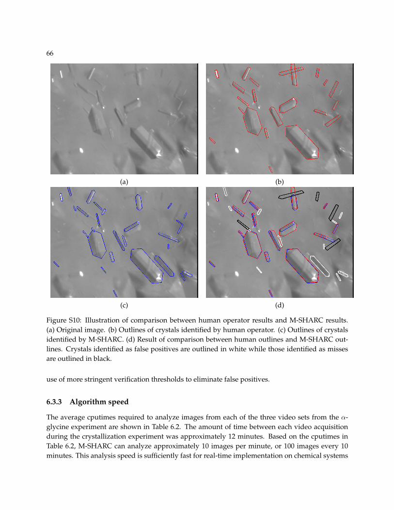
66

(a) (b)

(c) (d)

Figure S10: Illustration of comparison between human operator results and M-SHARC results.(a) Original image. (b) Outlines of crystals identified by human operator. (c) Outlines of crystalsidentified by M-SHARC. (d) Result of comparison between human outlines and M-SHARC out-lines. Crystals identified as false positives are outlined in white while those identified as missesare outlined in black.

use of more stringent verification thresholds to eliminate false positives.

6.3.3 Algorithm speed

The average cputimes required to analyze images from each of the three video sets from the α-glycine experiment are shown in Table 6.2. The amount of time between each video acquisitionduring the crystallization experiment was approximately 12 minutes. Based on the cputimes inTable 6.2, M-SHARC can analyze approximately 10 images per minute, or 100 images every 10minutes. This analysis speed is sufficiently fast for real-time implementation on chemical systems

67

Set Line Finding Group Finding Initialization Optimization Total1 2.6 (55) 1.2 (25) 0.2 (5) 0.7 (14) 4.82 3.3 (43) 3.3 (43) 0.3 (4) 0.7 (9) 7.63 3.3 (16) 15.4 (76) 0.4 (2) 1.0 (5) 20.2

Table 6.2: Average cputime required to analyze single image for three different image sets of in-creasing solids concentration. The first number in each number pair is the cputime in seconds.The second, parenthesized number gives the percentage of total cputime.

with crystallization dynamics similar to glycine.

The results presented in this paper are based on using a single wire-frame model. M-SHARC can be applied, however, using multiple models to represent different shape classes. Us-ing multiple models would affect the computational requirements in two ways. First, each ad-ditional model may require the identification of additional VIGs to serve as visual cues for thatmodel. However, the increase in computation time for the VIG identification stage may be smallbecause many VIGs are identified using the same set of logical decisions. For instance, to identifya C-triple, M-SHARC must determine whether a given triple of lines is connected at one or twojunctions. This same determination must be made to identify a C-square and an arrow. Second,the number of hypotheses would likely increase linearly with the number of models, resulting ina linear increase of computational requirements for the model initialization stage. In Table 6.2,the requirements for the initialization stage represent a small fraction of the total computationalrequirements, indicating that M-SHARC could accommodate several more models and remainsuitably fast for real-time implementation.

6.4 Conclusions

We have developed a model-based object recognition algorithm that is effective for extractingcrystal size and shape information from noisy, in situ crystallization images. The algorithm’saccuracy has been assessed by comparing its results with those obtained by manual, human anal-ysis of the images. At low solids concentrations, the algorithm identifies approximately half of thecrystals identified by humans, while at medium to high solids, the algorithm identifies approxi-mately one-third of the crystals. At low solids, false positives constitute approximately one-fifthof all identified crystals, while at medium to high concentrations the false positives constitute ap-proximately half of the identified crystals. Despite the misses and false positives, the algorithm’scumulative size distribution measurements compare favorably with measurements obtained byhumans but are biased towards larger particles. To improve the algorithm’s accuracy, furtherdevelopment should focus on the algorithm’s verification stage and on creating initialization rou-tines for additional viewpoint-invariant line groups. The algorithm is sufficiently fast to provideon-line measurements for typical cooling crystallization processes.

68

6.5 Acknowledgment

This material is based upon work supported by the National Science Foundation under Grant No.0540147. The authors gratefully acknowledge GlaxoSmithKline for providing the imaging systemused in this study and Dr. Karen Jones of the University of Wisconsin School of Pharmacy forXRPD analysis of the glycine crystals. The authors also express appreciation to Dr. Antonio Tor-ralba of the Massachussetts Institute of Technology Computer Science and Artificial IntelligenceLaboratory for enabling the use of the LabelMe database and Susan Larsen for her help in manu-ally tracing the crystals.

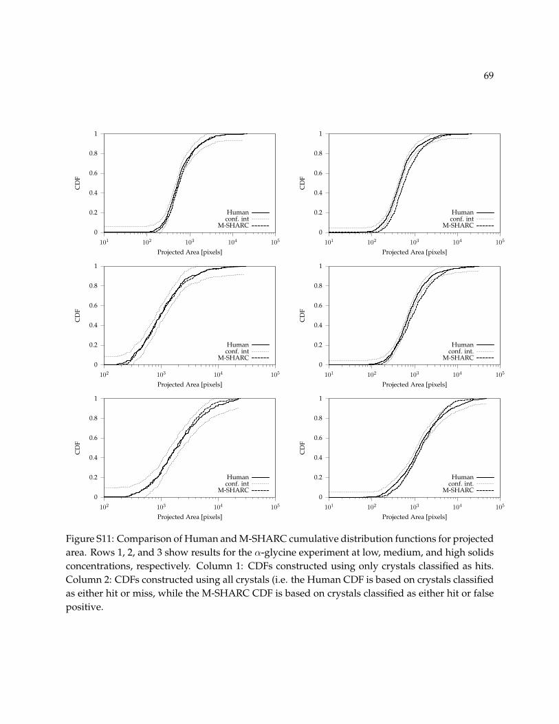
69

0

0.2

0.4

0.6

0.8

1

101 102 103 104 105

CD

F

Projected Area [pixels]

Humanconf. int

M-SHARC0

0.2

0.4

0.6

0.8

1

101 102 103 104 105

CD

F


Humanconf. int

M-SHARC

0

0.2

0.4

0.6

0.8

1

102 103 104 105

CD

F


Humanconf. int

M-SHARC0

0.2

0.4

0.6

0.8

1

101 102 103 104 105

CD

F


Humanconf. int.

M-SHARC

0

0.2

0.4

0.6

0.8

1

102 103 104 105

CD

F


Humanconf. int

M-SHARC0

0.2

0.4

0.6

0.8

1

101 102 103 104 105

CD

F


Humanconf. int.

M-SHARC

Figure S11: Comparison of Human and M-SHARC cumulative distribution functions for projectedarea. Rows 1, 2, and 3 show results for the α-glycine experiment at low, medium, and high solidsconcentrations, respectively. Column 1: CDFs constructed using only crystals classified as hits.Column 2: CDFs constructed using all crystals (i.e. the Human CDF is based on crystals classifiedas either hit or miss, while the M-SHARC CDF is based on crystals classified as either hit or falsepositive.

70

Figure S12: Results of linear feature detection for selected crystals missed by M-SHARC. Thepoor contrast for the crystals in row 1 is due to out-of-focus blur. The crystals in row 2 alsoexhibit poor contrast despite being seemingly in-focus. The crystals in row 3 show examplesof agglomeration. The crystals in row 4 may be identifiable given further development of M-SHARC’s correspondence and model parameter estimation routines described in Sections 6.2.4and 6.2.4.

71

Chapter 7

Statistical estimation of PSD fromimaging data7.1 Introduction

Particulate processes are ubiquitous in the chemical, food, and pharmaceutical industries. A fun-damental task for understanding and controlling particulate processes is measuring the particlesize distribution (PSD). Historically, this task has been accomplished by mechanical methods suchas sieving, but in the past several decades a wide variety of alternative technologies have beendeveloped to make PSD measurement more efficient and more accurate. These technologies in-clude, for example, forward laser light scattering and electrozone sensing. Unfortunately, thesemethods require sampling the particulate slurry, which is inconvenient and, in some cases, haz-ardous. Furthermore, obtaining a representative sample can be non-trivial. The difficulties asso-ciated with sampling have motivated the development of in situ sensors to measure PSD. Thesesensors include laser backscattering, ultrasonic spectroscopy, and in situ microscopy. Of thesein situ sensors, only microscopy allows direct observation of particle shape, which makes thismethod advantageous for systems in which the particles are non-spherical.

Two challenges must be addressed to use in situ microscopy for PSD measurement. Thefirst challenge is achieving image segmentation, or separating the objects of interest (e.g. the par-ticles) from the background. Methods for segmenting in situ images have been developed forcircular particles [99], arbitrarily-shaped particles [19], elliptical particles [47], needle-like parti-cles [59], and particles with shape that can be represented using a wireframe model [60].

The second challenge is to estimate the PSD given the size and shape information obtainedthrough successful image segmentation. Each segmented particle provides a single observation,which can be either censored or uncensored. A censored observation refers to an observation inwhich only partial information is obtained. For example, an observation of a particle touchingthe image border is censored because only a portion of the particle is visible. An observation ofa particle with one end partially occluded by another particle is also censored. An observationis uncensored only if the particle is enclosed entirely within the image frame, is not occluded byother particles, and is oriented in a plane perpendicular to the optical axis of the camera.

A natural approach to estimate the PSD is to count only those particles appearing entirelywithin the field of view, not touching the image boundary. This approach, called minus-sampling,introduces sampling bias because the probability of counting a particle depends on its size andshape. For example, a small particle randomly located in the image has a high probability of

72

appearing entirely within the field of view, while a sufficiently large particle randomly locatedin the image may have zero probability of appearing entirely within the field of view. Miles [72]presented the first treatment of spatial sampling bias, developing a minus-sampling estimator thatcorrects spatial sampling bias by weighting each observation by M−1, with M being related to thesampling probability of the observed particle. Miles derived formulas for M assuming a circularsampling region. Lantuejoul[57] extended Miles’ results by showing how to calculate M for arectangular sampling region.

The primary drawback of the Miles-Lantuejoul approach is that it uses only uncensoredobservations. If the size of the particles is large relative to the size of the image window, usingcensored observations (i.e. particles touching the image border) would be expected to result inimproved PSD estimation. The primary goal of this study is to develop a PSD estimator usingboth censored and uncensored observations and to evaluate the benefits and drawbacks of thisestimator relative to the Miles-Lantuejoul approach. We assume the censoring is due only to par-ticles touching the image border and not due to orientation or occlusion effects. A secondary goalis to develop practical methods for determining confidence intervals for the estimated PSD. Themethods developed in this study are intended for systems of high-aspect-ratio particles, which arecommonplace in the pharmaceutical and specialty chemical industries.

The paper is organized as follows. Section 8.2 describes previous work related to PSD esti-mation of high-aspect-ratio particles and describes the application of the Miles-Lantuejoul estima-tor. Section 8.3 presents the formulation of the maximum likelihood PSD estimator and Section 8.4describes the simulation studies used to test the estimator. Section 8.5 presents the results of thesesimulation studies, and Section 8.6 summarizes our findings. The full derivation of the maximumlikelihood estimator can be found in [58].

7.2 Previous work

PSD estimation for high-aspect-ratio particles using imaging-based measurements is related to theproblem of estimating the cumulative length distribution function H of line segments observedthrough a window, which has been investigated by several researchers. Laslett [61] was the firstto derive the log likelihood for this problem. Wijer [113] derived the non-parametric maximumlikelihood estimator (NPMLE) of H for a circular sampling region and an unknown orientationdistribution function K. For arbitrary convex sampling regions, Wijer shows how to estimateH assuming K is known. Van Der Laan[106] studies the NPMLE of H for the one-dimensionalline segment problem (i.e. all line segments have same orientation) for a non-convex samplingwindow, and Van Zwet[107] derives the NPMLE of H for the two-dimensional problem witha non-convex, highly irregular sampling region and known K. Svensson et al.[104] derive anestimator for a parametric length density function h using one-dimensional line segment datafrom a circular sampling region. Hall [45] derived an estimator for the intensity of a planar Poissonline segment process that is unbiased for any convex sampling region and any length distributionfunction. All of the above studies utilize both censored and uncensored observations. Baddeley [5]provides an excellent review of various spatial sampling estimation studies.

73

dF,h

b− dF,v

a− dF,h

dF,v

a

b

Mj

Lj

dF,v

dF,h

b− dF,v

a− dF,h

a

b

Lj

Mj

Figure S1: Depiction of methodology for calculating Miles-Lantuejoul M-values for particles ofdifferent lengths observed in an image of dimension b× a.

The goal of the current study is to estimate the particle size distribution f , which is relatedto but different than the cumulative distribution function H or corresponding density function h

for a line segment process. The PSD f(L) is the number of particles of length L per unit volumeand is related to H via the relation H(L ≤ l) =

∫ l0 f(L)dL/

∫∞0 f(L)dL. The approach commonly

used in practice to estimate the PSD from imaging-based measurements is the Miles-Lantuejoulmethod [72]. As there is some confusion amongst practitioners regarding the implementation ofthe Miles-Lantuejoul method, we describe the method here.

Let E2 be the Euclidean plane, and let D ⊂ E2 be a domain parameterized by (z, n, θn),in which z gives the center point of the domain, n gives the class, and θn is a vector giving theparameters necessary to completely specify a domain of class n. Let Q(x) ⊂ E2 be a samplingregion centered at x. For each domain D, define the set

Dα = x ∈ E2 : D ⊂ Q(x) (7.1)

Thus, Dα is a domain comprising all points at which the sampling region can be placed and en-close entirely the domain D.

Define MD = ADα, where A· denotes area. Let MDj, j = 1 . . . n be the M-valuescalculated for n observations of particles with lengths corresponding to size class i. Miles showedthat ρMLi =

∑j MDj is an unbiased estimator of ρi, the density of particles in size class i per

area, provided the minimum possible M-value for a particle in size class i is greater than zero.

In Miles’ original paper [72], he derived formulas for calculating M-values for arbitrarydomains assuming a circular sampling region. Later, Lantuejoul[57] extended Miles’ results byshowing how to calculate M for the rectangular sampling region typical of microscopy applica-tions. For an image of size a× b, the M-value of a particle is calculated by subtracting the verticaland horizontal Feret diameters of the particle (dF,v and dF,h) from, respectively, the vertical andhorizontal image dimensions b and a, as depicted in Figure S1.

74

7.3 Theory

7.3.1 PSD Definition

Consider a population of cylindrical or rod-like particles. The geometry of each particle is speci-fied in terms of the cylinder height h and radius r. Define the characteristic length for the popula-tion of particles as L = h.

Consider a slurry of volume V in which a solid phase of discrete particles is dispersedin a continuous fluid phase. Let f(L) denote the continuous PSD, or the number of particlesof characteristic length L per unit volume slurry. Number-based PSDs are typically measuredby discretizing the characteristic length scale into T non-overlapping bins or size classes. Wetherefore define the discrete PSD as

ρi =∫ Si+1

Si

f(l)dl, i = 1, . . . , T (7.2)

in which S = (S1, . . . , ST+1) is the vector of breaks between size classes.The relative PSD q is a vector with elements

qi =ρi∑Tj ρj

, i = 1, . . . , T (7.3)

In this paper, the term PSD is assumed to refer to the discrete, absolute PSD ρ unless specificallynoted otherwise.

7.3.2 Sampling model

The particle population is sampled using in situ imaging. Let VI ∈ V denote the imaging volume,and assume VI is a rectangular region of dimensions a× b× d, in which a is the horizontal imagedimension, b is the vertical image dimension, and d is the depth of field. a and b determine thefield of view, and we assume a ≥ b. A single random sample of the population consists of animage containing the two-dimensional projection of the portions of particles inside VI . We assumethe system is well-mixed such that the centroids of the particles are randomly and uniformlydistributed in space.

We assume the camera is positioned a fixed distance z0 from the imaging volume, and thatd z0. This assumption means the particles in the imaging volume are projected onto the imageplane according to the weak perspective projection model. In other words, the projected particlelengths measured in the image coordinate system can be related to the true projected particlelengths by applying a constant magnification factor m.

We assume all particles are oriented in a plane orthogonal to the camera’s optical axis. Thisassumption, together with the weak perspective assumption, essentially reduces the 3-D processto a 2-D process, thereby simplifying the analysis considerably. These assumptions are not usedonly for convenience, however, but rather to reflect the actual conditions under which in situimaging measurements are made in practice. To obtain useful in situ images in high solids con-centrations, the camera must have a small depth of field and be focused only a small depth into

75

the particulate slurry. It seems reasonable, therefore, to expect the shear flow at the slurry-sensorinterface to cause the particles to align orthogonal to the this interface, and thus orthogonal to thecamera’s optical axis.

7.3.3 Maximum likelihood estimation of PSD

Let Xk = (X1k, . . . , XTk) be a T -dimensional random vector in which Xik gives the number ofnon-border particles of size class i observed in image k. A non-border particle is a particle thatis completely enclosed within the imaging volume. A border particle, on the other hand, is onlypartially enclosed within the imaging volume such that only a portion of the particle is observable.For border particles, only the observed length (i.e. the length of the portion of the particle thatis inside the imaging volume) can be measured. Accordingly, we let Yk = (Y1k, . . . , YTk) be aT -dimensional random vector in which Yjk gives the number of border particles with observedlengths in size class j that are observed in image k. We denote the observed data, or the realizationsof the random vectors Xk and Yk, as xk and yk, respectively.

The particle population is represented completely by the vectors ρ = (ρi, . . . , ρT ) and S =(S1, . . . , ST+1) in which ρi represents the number of particles of size class i per unit volume andSi is the lower bound of size class i. Given the data x and y (the subscript k denoting the imageindex is removed for simplicity), the maximum likelihood estimator of ρ is defined as

ρb = arg maxρ

pXY (x1, y1, x2, y2, . . . , xT , yT |ρ) (7.4)

in which the subscript b indicates the use of border particle measurements and pXY is the jointprobability density for X and Y. In other words, we want to determine the value of ρ that maxi-mizes the probability of observing exactly x1 non-border particles of size class 1, y1 border particlesof size class 1, x2 non-border particles of size class 2, y2 border particles of size class 2, and so on.

A simplified expression for pXY can be obtained by noting that, at least at low solids con-centrations, the observations X1, Y1, . . . , XT , YT can be assumed to be independent. This as-sumption means that the observed number of particles of a given size class depends only on thedensity of particles in that same size class. At high solids concentrations, this assumption seemsunreasonable because the number of particle observations in a given size class is reduced dueto occlusions by particles in other size classes. At low concentrations, however, the likelihoodof occlusion is low. The independence assumption does not imply that the observations are notcorrelated. Rather, the assumption implies that any correlation between observations is due totheir dependence on a common set of parameters. As an example, if we observe a large num-ber of non-border particles, we would expect to also observe a large number of border particles.This correlation can be explained by noting that the probability densities for both border and non-border observations depend on a common parameter, namely, the density of particles. Given theindependence assumption, we express the likelihood function L(ρ) as

L(ρ) = pXY =T∏

i=1

pXi(xi|ρ)T∏

j=1

pYj (yj |ρ) (7.5)

76

in which pXi and pYj are the probability densities for the random variables Xi and Yj . The loglikelihood is defined as l(ρ) = log L(ρ). Maximizing the likelihood function is equivalent to min-imizing the log likelhood. Using Equation (A.2), the estimator in Equation (A.1) can therefore bereformulated as

ρb = arg minρ

T∑i=1

− log pXi(xi|ρ)−T∑

j=1

log pYj (yj |ρ) (7.6)

The probability densities pXi and pYj can be derived given the particle geometry and thespatial and orientational probability distributions. In [58], pXi and pYj are derived assuming theparticles have needle-like geometry, are uniformly distributed in space, and are uniformly dis-tributed in orientation. These derivations show that Xi ∼ Poisson(mXi), or that Xi has a Poissondistribution with parameter mXi = ρiαi, in which αi is a function of the field of view, depth offield, and the lower and upper bounds of size class i. Furthermore, Yj ∼ Poisson(mYj ), in whichmYj =

∑Ti=1 ρiβij

To extend the analysis to data collected from N images, we define two new random vectorsXΣ and YΣ for which XΣi =

∑Nk=1 Xik and YΣj =

∑Nk=1 Yjk. Here, the subscript k denotes the

image index. Given that Xik ∼ Poisson(mXi), it can be shown that XΣi ∼ Poisson(NmXi) [12, p.440]. Likewise, YΣj ∼ Poisson(NmYj ).

Differentiating Equation (A.3) with respect to ρ and equating with zero results in a set ofcoupled, nonlinear equations for which an analytical solution is not apparent. Equation (A.3) issolved using MATLAB’s nonlinear optimization solver FMINCON with initial values obtainedfrom Equation (7.7).

If the border particles are ignored, the estimator reduces to

ρ = arg minρ

T∑i=1

(− log pXi(xi|ρ))

In this case, we can solve for ρ analytically:

ρi =Xi

αi, i = 1, . . . , T (7.7)

The probability density for this estimator can be computed analytically as

pρi(ρi) = pρi(Xi/αi) = pXi(xi) (7.8)

with xi being a non-negative integer. It is straightforward to show that this estimator has thefollowing properties:

E[ρi] = ρi

V ar[ρi] = ρi/αi

For the case of multiple images, the maximum likelihood estimate is given by

ρi =XΣi

Nαi, i = 1, . . . , T (7.9)

77

which has the following properties:

E[ρi] = ρi

V ar[ρi] = ρi/(Nαi)

7.3.4 Confidence Intervals

Let χ = Z1,Z2, . . . ,ZN denote a dataset of N images, with Zk = (Xk,Yk) containing the datafor both border and non-border measurements for image k. Let Z1,Z2, . . . ,ZN be independentand identically distributed (i.i.d.) with distribution function F . Let F be the empirical distribu-tion function of the observed data. Let R(χ, F ) be a random vector giving the PSD estimatedusing either Miles-Lantuejoul or maximum likelihood. To construct confidence intervals for theestimated PSD, we require the distribution of R(χ, F ). This distribution, called the sampling dis-tribution, is unknown because F is unknown, being a function of the unknown PSD ρ. As N →∞,the limiting distribution of the maximum likelihood estimates is a multivariate normal with meanρ and covariance I(ρ)−1, where I(ρ) is the Fisher information matrix, defined as

I(ρ) = −E[l′′(ρ)]

in which l′′(ρ) is a T ×T matrix with the (i, j)th element given by ∂2l(ρ)∂ρi∂ρj

. Approximate confidenceintervals for individual parameter estimates can be calculated as ρi = ρi±σizα in which σi is the ithdiagonal element of the observed Fisher information matrix −l′′(ρ) and zα gives the appropriatequantile from the standard normal distribution for the confidence level α.

Given that the underlying distributions for Xk and Yk are Poisson, we expect the samplingdistributions to be non-normal in general. We therefore use bootstrapping [40, p.253] to approxi-mate the distribution of R(χ, F ) and construct confidence intervals. Let χ∗ = Z∗

1, . . . ,Z∗N denote

a bootstrap sample of the dataset χ. The elements of χ∗ are i.i.d. with distribution function F . Inother words, χ∗ is obtained by sampling χ N times where, for each of the N samples, the probabil-ity of selecting the data Zk is 1/N. We denote a set of B bootstrap samples as χ∗l = Z∗

l1, . . . ,Z∗lN

for l = 1, . . . , B. The empirical distribution function of R(χ∗l , F ) for l = 1, . . . , B approximates thedistribution function of R(χ, F ), enabling confidence intervals to be constructed.

For R(χ, F ) = ρ, the distribution function of R(χ∗, F ) is derived analytically using Equa-tion (7.8). For R(χ, F ) = ρb and R(χ, F ) = ρML, the distribution of R(χ∗, F ) is estimated usingB = 1000 bootstrap samples. The confidence intervals are obtained using the percentile method,which consists of reading the appropriate quantiles from the cumulative distribution of R(χ∗, F ).To calculate confidence intervals using the normal approximation, the observed Fisher informa-tion matrix −l′′(ρ), also called the Hessian, must be calculated. The (i, j)th element of this matrixis given by

− ∂l(ρ)∂ρi∂ρj

=XΣi

ρ2i

δij +T∑k

βjkβikYΣk

m2Yk

(7.10)

78

7.4 Simulation methods

To investigate the performance of the maximum likelihood estimator relative to the standardMiles-Lantuejoul approach, these estimators were applied in several case studies. In each casestudy, 1000 simulations were carried out. Each simulation consists of generating a set of artifi-cial images and applying the estimators to the particle length measurements obtained from theseimages. To generate an artificial image, we simulate the particle population in a local regionsurrounding the imaging volume VI . In this region, we model the particle population as a three-dimensional stochastic process Φ = (Xwi, Li,Θzi) on R3 × R+ × (−π/2, π/2] for i = 1, . . . , Nc.Xwi = (Xwi, Ywi, Zwi) gives the location of the centroid for particle i in the world coordinateframe, Li gives the length, Θzi gives the orientation around the z-axis of the world coordinateframe, and Nc gives the number of particles. Xwi, Li, Θzi, and Nc are distributed independently ofeach other. Xwi, Ywi, Zwi, and Θzi are distributed uniformly on [xmin, xmax], [ymin, ymax], [zmin, zmax],and (−π/2, π/2], respectively. Li has probability density function p(L). Nc has a Poisson distribu-tion with parameter λ = Nc(xmax − xmin)(ymax − ymin)/ab, in which Nc is the expected number ofcrystals per image, calculated from the PSD using

Nc = VI

∫ ∞

0f(l)dl

The size of the local region surrounding the imaging volume is defined by (xmin, xmax) = (−0.5Lmax, a+0.5Lmax) and (ymin, ymax) = (−0.5Lmax, b + 0.5Lmax), in which Lmax is defined as the size of thelargest particle in the population. If Lmax does not have a well-defined value, such as when thesimulated density function p(L) is normal, Lmax is assigned the value corresponding to the 0.997thquantile of the simulated distribution function.

Each particle has a cylindrical geometry with height Li and radius r, where r is assumedto be constant. Each particle is a convex, three-dimensional domain Pi ∈ V . To model the imagingprocess, Pi is projected onto an imaging plane using a camera model. This projection is computedby first applying rigid-body rotations and translations to change each point Xw in Pi from theworld coordinate frame to the camera coordinate frame:

Xc = RzRyRxXw + T (7.11)

in which Rz, Ry, and Rx are rigid-body rotation matrices, which are functions of the in-planeorientation θz and the orientations in depth θy and θx, respectively. T = (tx, ty, tz) is a translationvector. Next, each point is projected onto the image plane according to some imaging model.Under perspective projection, the transformation from a 3-D point Xc = (Xc, Yc, Zc) in cameracoordinates to an image point xc = (xc, yc) is given by

xc =fc

ZcXc, yc =

fc

ZcYc (7.12)

in which fc is the focal length of the camera. Figure S2 depicts the perspective projection of a cylin-drical particle onto the image plane. Finally, to model CCD imaging, the image plane coordinates

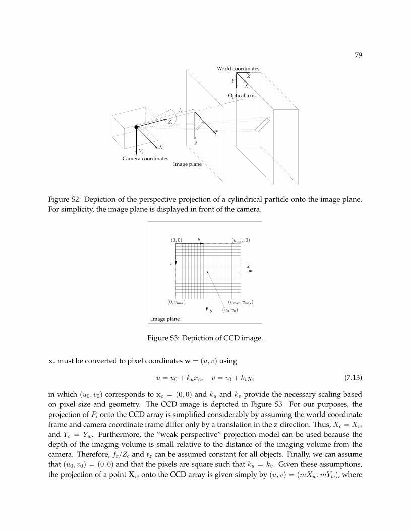
79

y

x

Zc

Optical axis

fc

Yc

Xc

Image plane

YX

Z

World coordinates

Camera coordinates

Figure S2: Depiction of the perspective projection of a cylindrical particle onto the image plane.For simplicity, the image plane is displayed in front of the camera.

x

y

Image plane

v

u

(u0, v0)

(umax, 0)

(0, vmax) (umax, vmax)

(0, 0)

Figure S3: Depiction of CCD image.

xc must be converted to pixel coordinates w = (u, v) using

u = u0 + kuxc, v = v0 + kvyc (7.13)

in which (u0, v0) corresponds to xc = (0, 0) and ku and kv provide the necessary scaling basedon pixel size and geometry. The CCD image is depicted in Figure S3. For our purposes, theprojection of Pi onto the CCD array is simplified considerably by assuming the world coordinateframe and camera coordinate frame differ only by a translation in the z-direction. Thus, Xc = Xw

and Yc = Yw. Furthermore, the “weak perspective” projection model can be used because thedepth of the imaging volume is small relative to the distance of the imaging volume from thecamera. Therefore, fc/Zc and tz can be assumed constant for all objects. Finally, we can assumethat (u0, v0) = (0, 0) and that the pixels are square such that ku = kv. Given these assumptions,the projection of a point Xw onto the CCD array is given simply by (u, v) = (mXw,mYw), where

80

m = kufc/Zc. The length of an observed particle therefore equals its length in pixels divided bythe factor m.

7.5 Results

Four different case studies were carried out to evaluate the effectiveness of the estimation meth-ods. Figure S5 shows example images generated for each of these case studies. Each of these im-ages has a horizontal image dimension of a=480 pixels and a vertical dimension of b=480 pixels.The first row displays four simulated images for monodisperse particles of length 0.5a with Nc=25crystals per image. The second row shows images of particles uniformly distributed on [0.1a 0.9a]with Nc=25. The third row shows images of particles normally-distributed with µ = 0.5a andσ = 0.4a/3 with Nc=25, and the fourth row shows example images for simulations of particlesuniformly-distributed on [0.1a 2.0a] with Nc=15.

81

Figure S4: Example images for simulations of various particle populations. Row 1: monodisperseparticles of length 0.5a, Nc=25. Row 2: particles uniformly distributed on [0.1a 0.9a]. Row 3:particles normally-distributed with µ = 0.5a and σ = 0.4a/3, Nc=25. Row 4: particles uniformly-distributed on [0.1a 2.0a], Nc=15.

82

0

50

100

150

200

250

300

20 22 24 26 28 30 32

coun

ts

ρi

MLE w/ bordersMLE

Miles

0

50

100

150

200

250

300

20 22 24 26 28 30 32

coun

ts

ρi

MLE w/ bordersMLE

Miles

(a) (b)

Figure S5: Comparison of estimated sampling distributions for absolute PSD for monodisperseparticles. Results based on 1000 simulations, 10 size classes, Nc=25. (a) Results for 10 im-ages/simulation. (b) Results for 100 images/simulation.

7.5.1 Case study 1: monodisperse particles of length 0.5a

In the first case study, the particle population consists of monodisperse particles of length 0.5a.The first row in Figure S5 shows example images from these simulations. The length scale is dis-cretized on [0.1a

√2a] into T=10 size classes with the fourth size class centered at 0.5a. The sam-

pling distributions for the various estimators are shown in Figure S5 for 1000 simulations using10 images/simulation and 100 images/simulation. Including the border particle measurementsprovides better estimates, as evidenced by the lower variance in the sampling distribution for ρb

relative to the other estimators. As a measure of the improvement gained by including the borderparticle measurements, we calculate the relative efficiency of ρbi

versus ρMLi for a given size classi as

eff(ρbi, ρMLi) =

MSE(ρMLi)MSE(ρbi

)(7.14)

in which MSE(T ) = var(T ) + [bias(T )]2 = E[(T − ρ)2] is the mean-squared error for estimator T .The MSE is estimated for size class i as

MSE(Ti) =1n

n∑j=1

(Tj − ρi)2 (7.15)

in which n is the number of simulations. The relative efficiency of the estimators appears relativelyindependent of the number of images per simulation, with values ranging between 3.5 and 4.0 asthe number of images per simulation is varied between 10 and 100. Thus, for this particular case,including the border particle measurements decreases the number of images required to obtain agiven accuracy by a factor of about four. For monodisperse systems in general, we would expectthe efficiency to be a monotonically increasing function of particle size.

Figure S6 demonstrates the effectiveness of the bootstrap approach for determining con-fidence intervals. Figure S6 is constructed by calculating bootstrap confidence intervals for 1000different simulations and determining what fraction of these confidence intervals contain the trueparameters for a given level of confidence, or α. The figure shows results for confidence intervals

83

00.10.20.30.40.50.60.70.80.9

1

0 0.1 0.2 0.3 0.4 0.5 0.6 0.7 0.8 0.9 1

frac

tion

insi

deα

inte

rval

α

expectedanalytical, MLEbootstrap, MLE

bootstrap, MLE w/ borders0

0.10.20.30.40.50.60.70.80.9

1

0 0.1 0.2 0.3 0.4 0.5 0.6 0.7 0.8 0.9 1

frac

tion

insi

deα

inte

rval

α


bootstrap, MLE w/ borders

(a) (b)

Figure S6: Fraction of confidence intervals containing the true parameter value versus confidencelevel. Results based on 1000 simulations, 10 size classes (results shown only for size class cor-responding to monodisperse particle size), Nc = 25. (a) Results for 10 images/simulation. (b)Results for 100 images/simulation.

based on the analytical sampling distribution of ρ (Equation (7.8) as well as sampling distributionsestimated using bootstrapping for both ρb and ρ. The fraction of confidence intervals containingthe true parameter corresponds closely to the expected value (i.e. the confidence level), even forthe case of only 10 images/simulation.

7.5.2 Case study 2: uniform distribution on [0.1a 0.9a]

In the second case study, the particle population consists of particles uniformly distributed on[0.1a 0.9a]. The second row in Figure S5 shows example images from these simulations. Thelength scale is discretized on [0.1a 0.9a] into T=10 size classes of equal size.

The efficiency of ρb relative to ρML, calculated using Equation (7.14), is plotted versus sizeclass in Figure S7. This plot indicates that including the border particle measurements does notappear to improve the estimation for the lower size classes but results in a significant increase inefficiency for the largest size class.

Figures S8 and S9 plot the fraction of bootstrap confidence intervals containing the truevalue of ρi for various size classes based on 100 images/simulation and 10 images/simulation.The bootstrap approach is effective for 100 images/simulation but underestimates the size of theconfidence interval for 10 images/simulation. Including the border particle measurements en-ables better determination of confidence intervals, particularly for the largest size class.

7.5.3 Case study 3: normal distribution

For the third case study, the particle population consists of particles with lengths distributed as anormal with µ = 0.5a and σ = 0.4a/3. The third row in Figure S5 shows example images fromthese simulations. The length scale is discretized on [µ − 3σ, µ + 3σ]=[0.1a 0.9a] into T=10 equi-

84

0.8

1

1.2

1.4

1.6

1.8

2

2.2

2.4

1 2 3 4 5 6 7 8 9 10

rela

tive

effic

ienc

y

size class

N=10N=30N=60

N=100

Figure S7: Relative efficiencies (eff(ρbi, ρMLi)) plotted versus size class for various numbers of

images per simulation: case study 2.

spaced size classes. Figure S10 illustrates the sampling distributions at the various size classes forρi. The x-y plane of Figure S10 shows the histogram generated for a normal distribution. The dis-crete sampling distributions, calculated using Equation (7.8), are plotted for each size class. Thisfigure indicates that the sampling distribution for a given size class can be adequately representedby a normal distribution provided the density of particles in that size class is sufficiently high.However, for the larger size classes, approximating the sampling distribution as a normal wouldlead to inaccurate confidence intervals.

85

0

0.1

0.2

0.3

0.4

0.5

0.6

0.7

0.8

0.9

1

0 0.1 0.2 0.3 0.4 0.5 0.6 0.7 0.8 0.9 1

frac

tion

insi

deα

inte

rval

α



0.1

0.2

0.3

0.4

0.5

0.6

0.7

0.8

0.9

1

0 0.1 0.2 0.3 0.4 0.5 0.6 0.7 0.8 0.9 1

frac

tion

insi

deα

inte

rval

α



(a) (b)

0

0.1

0.2

0.3

0.4

0.5

0.6

0.7

0.8

0.9

1

0 0.1 0.2 0.3 0.4 0.5 0.6 0.7 0.8 0.9 1

frac

tion

insi

deα

inte

rval

α



0.1

0.2

0.3

0.4

0.5

0.6

0.7

0.8

0.9

1

0 0.1 0.2 0.3 0.4 0.5 0.6 0.7 0.8 0.9 1

frac

tion

insi

deα

inte

rval

α



(c) (d)

Figure S8: Fraction of confidence intervals containing true parameter values for different confi-dence levels, N=100. (a) Size class 1 (smallest size class). (b) Size class 4. (c) Size class 7. (d) Sizeclass 10 (largest size class).

86

0

0.1

0.2

0.3

0.4

0.5

0.6

0.7

0.8

0.9

1

0 0.1 0.2 0.3 0.4 0.5 0.6 0.7 0.8 0.9 1

frac

tion

insi

deα

inte

rval

α



0.1

0.2

0.3

0.4

0.5

0.6

0.7

0.8

0.9

1

0 0.1 0.2 0.3 0.4 0.5 0.6 0.7 0.8 0.9 1

frac

tion

insi

deα

inte

rval

α



(a) (b)

0

0.1

0.2

0.3

0.4

0.5

0.6

0.7

0.8

0.9

1

0 0.1 0.2 0.3 0.4 0.5 0.6 0.7 0.8 0.9 1

frac

tion

insi

deα

inte

rval

α



0.1

0.2

0.3

0.4

0.5

0.6

0.7

0.8

0.9

1

0 0.1 0.2 0.3 0.4 0.5 0.6 0.7 0.8 0.9 1

frac

tion

insi

deα

inte

rval

α



(c) (d)

Figure S9: Fraction of confidence intervals containing true parameter values for different confi-dence levels, N=10. (a) Size class 1 (smallest size class). (b) Size class 4. (c) Size class 7. (d) Sizeclass 10 (largest size class).

87

01

23

45

67

02

46

8100

0.05

0.1

0.15

0.2

0.25

0.3

probability mass

absolute PSD size class

probability mass

Figure S10: Sampling distributions for the various size classes of a discrete normal distribution.N = 100.

Figure S11 plots eff(ρbi, ρMLi) for various numbers of images per simulation. Comparing

Figure S11 with Figure S7 indicates that the relative efficiency for a given size class is a function ofboth the size and the density of the particles in that size class.

7.5.4 Case study 4: uniform distribution on [0.4a 2.0a]

In the fourth case study, the particle population consists of particles uniformly distributed on [0.4a

2.0a]. The fourth row in Figure S5 shows example images from these simulations. The length scalewas discretized on [0.4a a] into T − 1 = 9 bins with the T th bin extending from a to Lmax. Lmax

was assumed unknown and estimated with initial value√

2a. That is, Equation (A.3) was solvedas before with the exception that the parameters mXi and mYj were updated at each iterationbased on the current estimate of Lmax. Figure S12 shows the sampling distributions for ρi for var-ious size classes, as well as the sampling distribution for Lmax. The MLE w/ borders approachis effective in estimating Lmax and the density of particles in the largest size class. It should beremembered, however, that the estimation is based on the assumption that the particles are uni-formly distributed across each size class. This assumption is suitable for finely discretized sizeclasses but is probably not suitable for the single, large, oversized size class. Thus, the estimatedvalue of Lmax should be used only as a rough estimate of the true value and as an indication for

88

1

1.1

1.2

1.3

1.4

1.5

1.6

1.7

1.8

1 2 3 4 5 6 7 8 9 10

rela

tive

effic

ienc

y

size class

N=10N=30N=60

N=100

Figure S11: Relative efficiencies (eff(ρbi, ρMLi)) plotted versus size class for various numbers of

images per simulation: case study 3.

0

20

40

60

80

100

0 0.2 0.4 0.6 0.8 1 1.2 1.4

MLE w/ bordersMLE

Miles

0

20

40

60

80

100

0 0.2 0.4 0.6 0.8 1 1.2 1.4

MLE w/ bordersMLE

Miles

0

20

40

60

80

100

0 0.2 0.4 0.6 0.8 1 1.2 1.4

MLE w/ bordersMLE

Miles

0

20

40

60

80

100

0 2 4 6 8 10 12

MLE w/ bordersMLE

Miles

0

20

40

60

80

100

1.4 1.6 1.8 2 2.2 2.4 2.6

MLE w/ borders

Figure S12: Comparison of sampling distributions for absolute PSD for particles distributed uni-formly on [0.4a 2.0a]. Results based on 200 simulations, 100 images/simulation, 10 size classes,Nc=15. (a) Size class 1. (b) Size class 5. (c) Size class 9. (d) Size class 10. (e) Lmax.

the appropriateness of the camera magnification.

89

7.6 Conclusion

The maximum likelihood estimator for imaging-based PSD measurement of zero-width, needle-like particles has been derived using both censored and uncensored observations (i.e. border andnon-border particles). The performance of the estimator has been compared with the standardMiles-Lantuejoul approach using four case studies that highlight several advantages of the MLEapproach. The case studies indicate that MLE is more efficient than Miles-Lantuejoul, particularlyif the particle population is monodisperse or contains particles that are large relative to the size ofthe image. Furthermore, MLE can estimate the number density of over-sized particles (particlesbigger than the image dimension) along with the size Lmax of the largest particle while the Miles-Lantuejoul approach can be applied only for particles smaller than the image dimension.

The limitations of the MLE approach should also be discussed. The primary limitation ofthe MLE derived in this paper is due to the assumption that the particles have needle-like geom-etry. The Miles-Lantuejoul approach, on the other hand, can be applied to a much wider class ofgeometries. Secondly, the MLE approach requires the solution of a nonlinear optimization prob-lem. Thus, confidence interval determination by bootstrapping can be computationally-intensive.Finally, it should be noted that the MLE estimates related to over-sized particles are obtained bymaking the rather unrealistic assumption that over-sized particles are uniformly distributed inlength on [a Lmax]. The estimates related to over-sized particles are therefore biased in general butmay be useful for identifying whether or not the camera magnification is suitable for the givensystem.

Several areas for future work are evident. Choosing the optimal number, location, andsize of bins for constructing histograms should be addressed. Integrating measurements takenat multiple scales or magnifications is also important. For systems of high-aspect-ratio particles,incorporating the width of border particles into the estimation could lead to increased efficiencyby narrowing down the number of size classes to which a border particle may correspond. Meth-ods for estimating the PSD when occlusion or overlap effects are not negligible are necessary forsystems at high solids concentrations.

7.7 Acknowledgment

This material is based upon work supported by the National Science Foundation under Grant No.0540147.

90

Chapter 8

Assessing the reliability ofimaging-based, number densitymeasurement8.1 Introduction

Advanced control of crystal shape, size distribution, and polymorphic form (internal lattice struc-ture) in suspension crystallization processes has been hindered by the limitations of available on-line sensors. High-speed, in situ video microscopy is a promising technology for measuring thesecritical solid-phase properties. Several challenges must be addressed to use in situ microscopyfor PSD measurement. The first challenge is achieving image segmentation, or separating the ob-jects of interest (e.g. the particles) from the background. Methods for segmenting in situ imageshave been developed for circular particles [99], arbitrarily-shaped particles [19], elliptical parti-cles [47], needle-like particles [59], and particles with shape that can be represented using a wire-frame model [60].

The second challenge is to estimate the PSD given the size and shape information obtainedthrough successful image segmentation. The estimation is complicated by the presence of twotypes of edge effects: sampling bias and censoring. Sampling bias occurs when the probabilityof observing an object depends on its size or shape. Sampling bias accompanies imaging-basedPSD measurement because particles that are large relative to the size of the image have a highprobability of intersecting the image boundary while smaller particles have a low probability ofintersecting the image boundary. Censoring occurs when only partial information is obtainedfor a given observation. For example, an observation of a particle touching the image borderreveals that the particle is at least as long as the observed length, but the true length is unknown.Miles [72] and Lantuejoul [57] derived an unbiased estimator of PSD that corrects sampling biasusing only uncensored observations. We [?] derived the maximum likelihood estimator for thePSD of high-aspect-ratio particles including censored observations. Both of these methods assumethe objects of interest are resting in a plane perpendicular to the optical axis of the camera. Ifthe particles are randomly oriented in three-dimensional space, the two-dimensional projectedlengths are less than or equal to the true lengths, resulting in another type of censoring for whichthese previous methods do not account. Baddeley [5] provides an excellent review of variousmethods for correcting edge effects under a variety of situations.

91

A third challenge lies at the interface of the two challenges just mentioned. The methodsfor PSD estimation in the presence of sampling bias and censoring are based on the assumptionthat image segmentation is perfect, or that every single particle appearing in the image is iden-tified correctly. Achieving perfect image segmentation is a realistic goal, however, only at lowsolids concentrations. At higher solids concentrations, a significant fraction of the particles maybe overlapping or occluded, which often results in these particles being missed by the automatedimage analysis algorithm. The density of particles is thus underestimated. The objective of thiswork is to address this third challenge by developing a semi-empirical, probabilistic model thatenables PSD estimation for imperfect image analysis. This paper also presents a descriptor thatcan be used to quantify the expected amount of particle overlap and thereby assess the reliabilityof the PSD estimate.

The paper is organized as follows. Section 8.2 presents previous work relevant to the scopeof this paper. Section 8.3 presents theory related to particle overlap probabilities, proposes a de-scriptor for measurement reliability, and presents an estimator for particle number density thataccounts for particle overlap. Section 8.4 describes the simulation studies used to determine theconditions for which SHARC gives an accurate PSD measurement. Section 8.5 presents the resultsof these simulation studies, and Section 8.6 summarizes our findings.

8.2 Previous Work

Armitage [4] was one of the first to investigate the effects of particle overlap on particle num-ber density estimation. Armitage derived formulas for the expected numbers of isolated clumps(groups of one or more overlapping particles) for circular and rectangular particles, and used theseformulas to estimate the mean clump size and number density of particles. Mack [68, 69] extendedArmitage’s results to three-dimensional particles of any convex shape, deriving formulas for theexpected numbers of clumps and isolated particles based on the perimeters and areas of the two-dimensional projections of the particles. Roach [91] summarized the work of Mack and Armitage,described several applications, and developed theory for specialized applications. Kellerer [56]was the first to account for edge effects and overlap simultaneously and derived a formula forthe expected number of clumps minus the number of enclosed voids (i.e. regions of the imagecompletely enclosed by particles). To model the complicated, random shapes that form due to therandom placement and overlap of simple geometric objects, the Boolean model [1, 6] can be used.

The methods cited above assume that a clear distinction can be made between the imagebackground and the objects of interest, or that the image can be segmented by simple threshold-ing. In some applications, however, more advanced image analysis is required, and modelingthe output of a complicated image analysis algorithm to enable statistical inference is non-trivial.For example, we previously developed a novel image analysis algorithm called SHARC that au-tomatically extracts particle size information from in situ images of needle-like crystals [59]. Us-ing images acquired during a pharmaceutical crystallization experiment, we demonstrated thatSHARC’s PSD measurements are consistent with measurements obtained through manual, hu-man analysis of the images, provided the images are acquired under suitable conditions. As a

92

model-based vision algorithm, SHARC can successfully identify overlapped particles providedthe degree of overlap is minor. Initial studies have shown that the methods cited above do notadequately model the output of the SHARC algorithm. In this work, we extend these methods toenable statistical inference for SHARC’s output. We expect the methodology developed here to beapplicable to other situations in which advanced image analysis is necessary to extract informa-tion from noisy images.

8.3 Theory

8.3.1 Particulate system definition

Consider a slurry of volume V in which a solid phase of discrete particles is dispersed in a contin-uous fluid phase. Let ρc be the solid phase density (mass solid/volume solid) and MT the slurrydensity (mass solid/volume slurry), or solids concentration. The volume solids concentration(volume solid/volume slurry) is given by MT /ρc. Let L be the characteristic length of a particleand define a shape factor kv such that the volume of a single particle is given by kvL

3. Let f(L)denote the PSD, or the number of particles of characteristic length L per unit volume slurry. Theith moment of the PSD is denoted µi =

∫∞0 f(L)LidL. Given the PSD, the slurry density can be

calculated as MT = ρckvµ3 assuming kv is independent of length. The zeroth moment, µ0, equalsthe number of particles per unit volume slurry. For a monodisperse system in which all particleshave the same length l, µ0 = MT /ρckvl

3.

8.3.2 Sampling and measurement definitions

Let VI ∈ V denote an imaging volume, and let I denote an image created by perspective projec-tion of VI onto a two-dimensional image plane. Let a and b denote the horizontal and verticaldimensions of VI , or the field of view, and let d denote the depth dimension of VI , or the depthof field. Thus, the volume of VI is given by abd, and the average number of particles per image isgiven by Nc = µ0abd.

Number-based PSDs are typically measured by discretizing the characteristic length scaleinto T non-overlapping bins or size classes. We therefore define the discrete PSD as

ρi =∫ Si+1

Si

f(l)dl, i = 1, . . . , T (8.1)

in which S = (S1, . . . , ST+1) is the vector of breaks between size classes. In this work, we consideronly monodisperse populations, so we represent the PSD for a given system using a single scalarvalue ρ. For a monodisperse system, ρ equals the number density.

8.3.3 Descriptor for number density reliability

Our goal is to estimate the number density of particles, and our hypothesis is that the quality orreliability of the estimate will correlate with the amount of particle overlap. We therefore want

93

to quantify the amount of particle overlap observed in the acquired images. We can calculatethe probability that a given particle will be overlapped by other particles as follows. Considera population of n identical particles randomly located within a system volume VS . The numberdensity of particles is given by n/VS . Let the particles be projected orthogonally onto a plane ofarea AS , giving a particle density per unit area of ρA = n/AS . Let K be a random variable givingthe number of times a given particle’s projection is overlapped by other particles’ projections.Assuming AS is sufficiently large that edge effects are negligible, the probability that the projectionof a given particle will be overlapped by the projection of a second, given particle is povp = Ω/AS ,in which Ω denotes the admissible area, or the area of the region inside which the second particle’sprojection overlaps the first particle’s projection. Thus, the probability that a given particle willbe overlapped by k particles is given by the binomial distribution with n Bernoulli trials and theprobability of success in each trial given by povp,

pK(k) =

(n

k

)pk

ovp(1− povp)n−k (8.2)

As n →∞ with ρA = n/AS constant, the binomial distribution converges to the Poisson distribu-tion with parameter λ = ρAΩ.

pK(k) =e−λλk

k!(8.3)

Thus, the probability that a given particle will be completely isolated is given by piso = pK(0) =exp(−ρAΩ).

As already mentioned, we expect the reliability of the PSD estimate to correlate with parti-cle overlap. Therefore, as an indicator of the reliability of the PSD estimate, we define the param-eter D as

D = − log(piso) = ρAΩ (8.4)

The area density ρA can be calculated as ρA = µ0d. The admissible area Ω depends on the particlegeometry. To illustrate how the admissible area can be calculated, consider the rectangular particleof length l and width w in the center of Figure S1. Next, consider a second particle of identicaldimensions placed in the image with orientation θ. If the midpoint of the second particle is placedanywhere inside the shaded region in Figure S1, the first and second particles overlap. This factis illustrated in Figure S1(b) using the various particles placed around the border of the shadedarea. Using straightforward geometric relationships (see Figure S1(a)), the area Aovp of this shadedregion can be shown to be

Aovp = (w(1 + sin θ) + l cos θ)(l(1 + sin θ) + w cos θ)− l2 cos θ sin θ − w2 cos θ sin θ (8.5)

and Ω is obtained by integrating over θ

Ω = E[Aovp] =1π

∫ π/2

−π/2Aovpdθ =

2π

(l2 + w2 + lw(2 + π)

)(8.6)

in which a uniform distribution in orientation has been assumed.

94

l(1 + sin θ)+w cos θ

w

w sin θ

w cos θ

l cos θ

l sin θ

l

Aovp

w(1 + sin θ) + l cos θ

w

l

Aovp

(a) (b)

Figure S1: Geometric representation of region in which particles of specific orientation and shapeoverlap.

Mack [68] (see also Roach [91, p.44]) derived a more general result that enables the calcu-lation of the admissible area Ω for any set of convex bodies of identical size and shape and havingrandom orientation. Mack’s surprisingly simple result gives Ω based on the area ap and perimetersp of a two-dimensional domain:

Ω = 2ap +s2p

2π(8.7)

8.3.4 Estimation of number density

Given our hypothesis that particle overlap is the primary cause of failure for image analysis-basedmeasurement, it seems reasonable to estimate the number density of particles based on the num-ber of completely isolated particles observed in the image. Letting X be a random variable givingthe number of observations of completely isolated, non-border particles, it can be shown that theprobability density for X is Poisson with parameter mX = ρANANB exp(−ρAΩ), in which N isthe number of images, ANB is the area of the region inside which a particle does not touch the im-age border, Ω is the admissible area defined above, and ρA is the area number density as definedabove. The maximum likelihood estimate of ρA is therefore

ρA = arg maxρA

e−mX mxX

x!(8.8)

in which x is the realization of X , or the measured number of isolated, non-border particles.The estimator given by Equation (8.8) is correct if the image analysis algorithm identi-

fies only isolated particles. Model-based image analysis algorithms, however, are designed toidentify the objects of interest even in the presence of overlap or occlusion. The number of par-ticles observed by a model-based image analysis algorithm is therefore greater than the number

95

of isolated particles, and Equation (8.8) can be expected to give bad estimates given such data.Assuming the number of particles identified by any given image analysis algorithm depends pri-marily on the amount of overlap, a reasonable model can be formulated based on the overlapmodel given above. Letting X denote the number of particles identified by an image analysisalgorithm, a reasonable form for the probability density of X would be Poisson with parametermX = ρANANB exp(−ρAΩθ), in which θ is an empirical parameter and the other variables are asdefined previously.

8.4 Simulation methods

This section describes the methods used to generate artificial images and analyze the images.

8.4.1 Artificial image generation

To generate an artificial image, we simulate the particle population in a local region surroundingthe imaging volume VI . In this region, we model the particle population as a three-dimensionalstochastic process Φ = (Xwi, Li,Θzi) on R3×R+×(−π/2, π/2] for i = 1, . . . , Nc. Xwi = (Xwi, Ywi, Zwi)gives the location of the centroid for particle i in the world coordinate frame, Li gives the length,Θzi gives the orientation around the z-axis of the world coordinate frame, and Nc gives the num-ber of particles. Xwi, Li, Θzi, and Nc are distributed independently of each other. Xwi, Ywi, Zwi,and Θzi are distributed uniformly on [xmin, xmax], [ymin, ymax], [zmin, zmax], and (−π/2, π/2], respec-tively. Li has probability density function p(L). Nc has a Poisson distribution with parameterλ = Nc(xmax − xmin)(ymax − ymin)/ab, in which Nc is the expected number of crystals per image,calculated from the PSD using

Nc = VI

∫ ∞

0f(l)dl

The size of the local region surrounding the imaging volume is defined by (xmin, xmax) = (−0.5Lmax, a+0.5Lmax) and (ymin, ymax) = (−0.5Lmax, b + 0.5Lmax), in which Lmax is defined as the size of thelargest particle in the population. If Lmax does not have a well-defined value, such as when thesimulated density function p(L) is normal, Lmax is assigned the value corresponding to the 0.997thquantile of the simulated distribution function.

Each particle is a convex, three-dimensional domain Pi ∈ V . To model the imaging process,Pi is projected onto an imaging plane using a camera model. This projection is computed by firstapplying rigid-body rotations and translations to change each point Xw in Pi from the worldcoordinate frame to the camera coordinate frame:

Xc = RzRyRxXw + T (8.9)

in which Rz, Ry, and Rx are rigid-body rotation matrices, which are functions of the in-planeorientation θz and the orientations in depth θy and θx, respectively. T = (tx, ty, tz) is a translationvector. Next, each point is projected onto the image plane according to some imaging model.

96

y

x

Zc

Optical axis

f

Yc

Xc

Image plane

YX

Z

World coordinates

Camera coordinates

Figure S2: Depiction of the perspective projection of a cylindrical particle onto the image plane.For simplicity, the image plane is displayed in front of the camera.

Under perspective projection, the transformation from a 3-D point Xc = (Xc, Yc, Zc) in cameracoordinates to an image point xc = (xc, yc) is given by

xc =fc

ZcXc, yc =

fc

ZcYc (8.10)

in which fc is the focal length of the camera. Figure S2 depicts the perspective projection of a cylin-drical particle onto the image plane. Finally, to model CCD imaging, the image plane coordinatesxc must be converted to pixel coordinates w = (u, v) using

u = u0 + kuxc, v = v0 + kvyc (8.11)

in which (u0, v0) corresponds to xc = (0, 0) and ku and kv provide the necessary scaling basedon pixel size and geometry. The CCD image is depicted in Figure S3. For our purposes, theprojection of Pi onto the CCD array is simplified considerably by assuming the world coordinateframe and camera coordinate frame differ only by a translation in the z-direction. Thus, Xc = Xw

and Yc = Yw. Furthermore, the “weak perspective” projection model can be used because thedepth of the imaging volume is small relative to the distance of the imaging volume from thecamera. Thus, fc/Zc and tz can be assumed constant for all objects. Finally, we can assume that(u0, v0) = (0, 0) and that the pixels are square such that ku = kv. Given these assumptions, theprojection of a point Xw onto the CCD array is given simply by (u, v) = (mX1,mY1), wherem = kufc/Zc.

The information required to generate an artificial image includes the image dimensions a

and b and magnification m, the length distribution p(L), the aspect ratio AR, and the number ofparticles per image λ. For simulations at a given solids concentration MT , λ is calculated as

λ =MT abd

ρc

∫∞0 p(L)kvL3dL

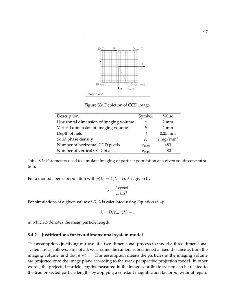
97

x

y

Image plane

v

u

(u0, v0)

(umax, 0)

(0, vmax) (umax, vmax)

(0, 0)

Figure S3: Depiction of CCD image.

Description Symbol ValueHorizontal dimension of imaging volume a 2 mmVertical dimension of imaging volume b 2 mmDepth of field d 0.25 mmSolid phase density ρc 2 mg/mm3

Number of horizontal CCD pixels umax 480Number of vertical CCD pixels vmax 480

Table 8.1: Parameters used to simulate imaging of particle population at a given solids concentra-tion.

For a monodisperse population with p(L) = δ(L− l), λ is given by

λ =MT abd

ρckvl3

For simulations at a given value of D, λ is calculated using Equation (8.4):

λ = D/povp(L) + 1

in which L denotes the mean particle length.

8.4.2 Justifications for two-dimensional system model

The assumptions justifying our use of a two-dimensional process to model a three-dimensionalsystem are as follows. First of all, we assume the camera is positioned a fixed distance z0 from theimaging volume, and that d z0. This assumption means the particles in the imaging volumeare projected onto the image plane according to the weak perspective projection model. In otherwords, the projected particle lengths measured in the image coordinate system can be related tothe true projected particle lengths by applying a constant magnification factor m, without regard

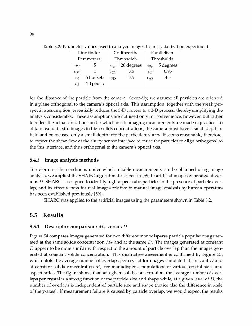
98

Table 8.2: Parameter values used to analyze images from crystallization experiment.Line finder Collinearity ParallelismParameters Thresholds Thresholds

n∇ 5 εθC20 degrees εθP

5 degreesε|∇| 1 εEP 0.5 εQ 0.85nb 6 buckets εPD 0.5 εAR 4.5εA 20 pixels

for the distance of the particle from the camera. Secondly, we assume all particles are orientedin a plane orthogonal to the camera’s optical axis. This assumption, together with the weak per-spective assumption, essentially reduces the 3-D process to a 2-D process, thereby simplifying theanalysis considerably. These assumptions are not used only for convenience, however, but ratherto reflect the actual conditions under which in situ imaging measurements are made in practice. Toobtain useful in situ images in high solids concentrations, the camera must have a small depth offield and be focused only a small depth into the particulate slurry. It seems reasonable, therefore,to expect the shear flow at the slurry-sensor interface to cause the particles to align orthogonal tothe this interface, and thus orthogonal to the camera’s optical axis.

8.4.3 Image analysis methods

To determine the conditions under which reliable measurements can be obtained using imageanalysis, we applied the SHARC algorithm described in [59] to artificial images generated at var-ious D. SHARC is designed to identify high-aspect-ratio particles in the presence of particle over-lap, and its effectiveness for real images relative to manual image analysis by human operatorshas been established previously [59].

SHARC was applied to the artificial images using the parameters shown in Table 8.2.

8.5 Results

8.5.1 Descriptor comparison: MT versus D

Figure S4 compares images generated for two different monodisperse particle populations gener-ated at the same solids concentration MT and at the same D. The images generated at constantD appear to be more similar with respect to the amount of particle overlap than the images gen-erated at constant solids concentration. This qualitative assessment is confirmed by Figure S5,which plots the average number of overlaps per crystal for images simulated at constant D andat constant solids concentration MT for monodisperse populations of various crystal sizes andaspect ratios. The figure shows that, at a given solids concentration, the average number of over-laps per crystal is a strong function of the particle size and shape while, at a given level of D, thenumber of overlaps is independent of particle size and shape (notice also the difference in scaleof the y-axes). If measurement failure is caused by particle overlap, we would expect the results

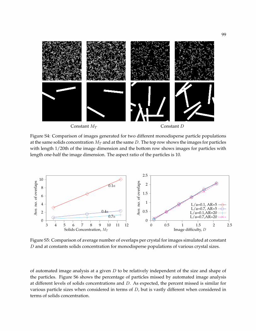
99

Constant MT Constant D

Figure S4: Comparison of images generated for two different monodisperse particle populationsat the same solids concentration MT and at the same D. The top row shows the images for particleswith length 1/20th of the image dimension and the bottom row shows images for particles withlength one-half the image dimension. The aspect ratio of the particles is 10.

0

2

4

6

8

10

3 4 5 6 7 8 9 10 11 12

Ave

.no.

ofov

erla

ps

Solids Concentration, MT

0.1a

0.4a

0.7a0

0.5

1

1.5

2

2.5

0 0.5 1 1.5 2 2.5

Ave

.no.

ofov

erla

ps

Image difficulty, D

L/a=0.1, AR=5L/a=0.7, AR=5L/a=0.1,AR=20L/a=0.7,AR=20

Figure S5: Comparison of average number of overlaps per crystal for images simulated at constantD and at constants solids concentration for monodisperse populations of various crystal sizes.

of automated image analysis at a given D to be relatively independent of the size and shape ofthe particles. Figure S6 shows the percentage of particles missed by automated image analysisat different levels of solids concentrations and D. As expected, the percent missed is similar forvarious particle sizes when considered in terms of D, but is vastly different when considered interms of solids concentration.

100

0

20

40

60

80

100

0 1 2 3 4 5 6

Perc

entm

isse

d

Solids concentration, MT

L/a = 0.10.40.7

0

20

40

60

80

100

0 0.5 1 1.5 2

Perc

entm

isse

d

Image difficulty, D

L/a = 0.10.40.7

(a) (b)

Figure S6: Comparison of percentage of particles missed by automated image analysis for imagessimulated at constant D and at constants solids concentration for monodisperse populations ofvarious crystal sizes.

8.5.2 Estimation of number density

In this section, we examine different methods for estimating the number density ρ. We first ex-amine the behavior of the Miles-Lantuejoul estimator, which corrects for edge effects but not forparticle overlap. Next, we examine the performance of the maximum likelihood estimator pre-sented in Section 8.3.4. The estimators are applied to data acquired by analyzing images usingSHARC. Example images for various levels of D and three different particle sizes (L/a = 0.1, 0.3,and 0.5) are shown in Figure S5.

Miles-Lantuejoul method

Figure S8 shows the ratio of the estimated and true number density as a function of D for var-ious particle sizes. In this figure, the number density of particles is estimated using the Miles-Lantuejoul method [72, 57], which does not account for overlap. The particle size and shapemeasurements are obtained using the SHARC algorithm. The estimator’s bias increases with D,or as the amount of overlap increases. Given the well-behaved and relatively size-independentcorrelation between ρ/ρ and D, one may attempt to correct ρ based on an estimated value of D.The result of such an approach is shown in Figure S8(b). The number density estimates for thisfigure are given by

ρ =ρML

g(D)

in which ρML denotes the Miles-Lantuejoul estimate, D is an estimate of D given by D = ρMLΩ,and g is an empirical function generated by fitting g(D) = exp(−θD) to the data in Figure S8(a).The parameter θ is determined using nonlinear least-squares minimization. This approach is inef-fective because D cannot be estimated independently of ρ, so both D and ρ are underestimated.

101

0.1

1.0

2.0

3.0

4.0

5.0

6.0

Figure S7: Examples of synthetic images generated at various D. The first, second, and thirdcolumn correspond to particle sizes L/a = 0.1, 0.3, and 0.5, respectively.

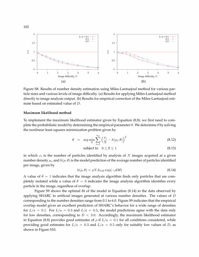
102

0

0.5

1

1.5

2

0 1 2 3 4 5 6

ρ/ρ

Image difficulty, D

L/a = 0.10.30.5

0

0.5

1

1.5

2

0 1 2 3 4 5 6

ρ/ρ

Image difficulty, D

L/a = 0.10.30.5

(a) (b)

Figure S8: Results of number density estimation using Miles-Lantuejoul method for various par-ticle sizes and various levels of image difficulty. (a) Results for applying Miles-Lantuejoul methoddirectly to image analysis output. (b) Results for empirical correction of the Miles-Lantuejoul esti-mate based on estimated value of D.

Maximum likelihood method

To implement the maximum likelihood estimator given by Equation (8.8), we first need to com-plete the probabilistic model by determining the empirical parameter θ. We determine θ by solvingthe nonlinear least squares minimization problem given by

θ = arg minθ

nd∑i=1

(xi

N− h(ρi, θ)

)2(8.12)

subject to 0 ≤ θ ≤ 1 (8.13)

in which xi is the number of particles identified by analysis of N images acquired at a givennumber density ρi, and h(ρ, θ) is the model prediction of the average number of particles identifiedper image, given by

h(ρ, θ) = ρNANB exp(−ρΩθ) (8.14)

A value of θ = 1 indicates that the image analysis algorithm finds only particles that are com-pletely isolated while a value of θ = 0 indicates the image analysis algorithm identifies everyparticle in the image, regardless of overlap.

Figure S9 shows the optimal fit of the model in Equation (8.14) to the data observed byapplying SHARC to artificial images generated at various number densities. The values of D

corresponding to the number densities range from 0.1 to 6.0. Figure S9 indicates that the empiricaloverlap model gives an excellent prediction of SHARC’s behavior for a wide range of densitiesfor L/a = 0.1. For L/a = 0.3 and L/a = 0.5, the model predictions agree with the data onlyfor low densities, corresponding to D < 3.0. Accordingly, the maximum likelihood estimatorin Equation (8.8) provides good estimates of ρ if L/a = 0.1 for all conditions considered, whileproviding good estimates for L/a = 0.3 and L/a = 0.5 only for suitably low values of D, asshown in Figure S10.

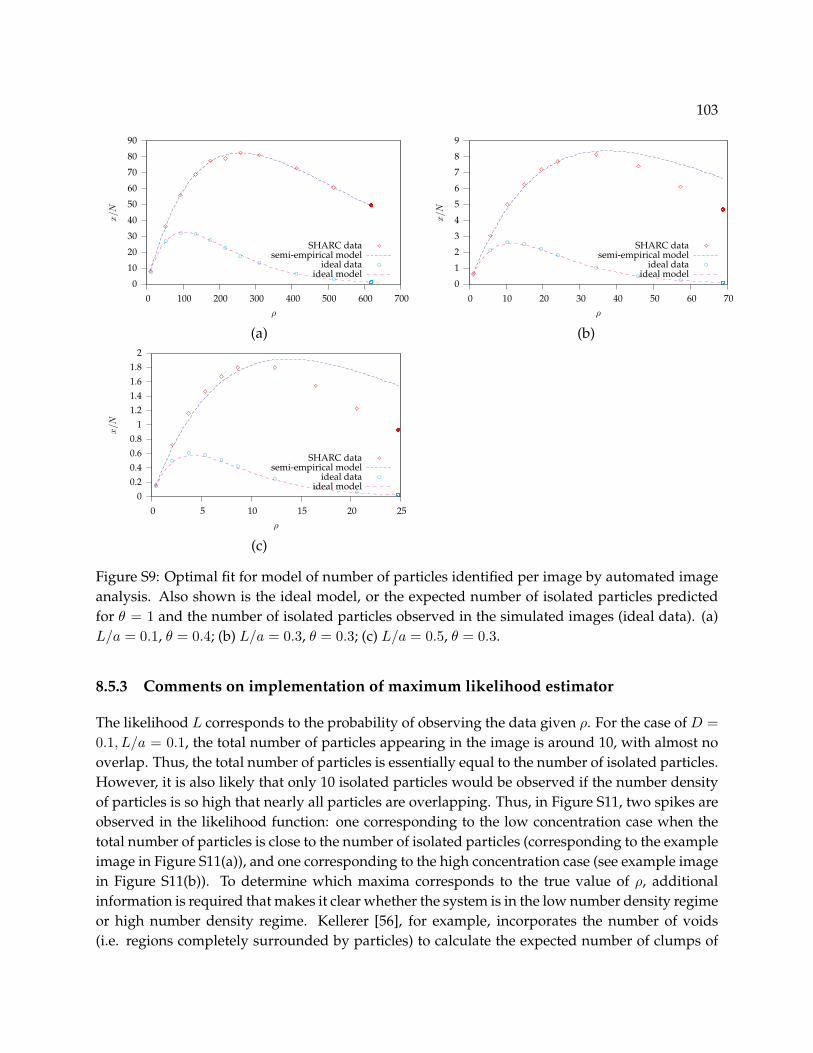
103

0

10

20

30

40

50

60

70

80

90

0 100 200 300 400 500 600 700

x/N

ρ

SHARC datasemi-empirical model

ideal dataideal model

0

1

2

3

4

5

6

7

8

9

0 10 20 30 40 50 60 70

x/N

ρ



(a) (b)

00.20.40.60.8

11.21.41.61.8

2

0 5 10 15 20 25

x/N

ρ



(c)

Figure S9: Optimal fit for model of number of particles identified per image by automated imageanalysis. Also shown is the ideal model, or the expected number of isolated particles predictedfor θ = 1 and the number of isolated particles observed in the simulated images (ideal data). (a)L/a = 0.1, θ = 0.4; (b) L/a = 0.3, θ = 0.3; (c) L/a = 0.5, θ = 0.3.

8.5.3 Comments on implementation of maximum likelihood estimator

The likelihood L corresponds to the probability of observing the data given ρ. For the case of D =0.1, L/a = 0.1, the total number of particles appearing in the image is around 10, with almost nooverlap. Thus, the total number of particles is essentially equal to the number of isolated particles.However, it is also likely that only 10 isolated particles would be observed if the number densityof particles is so high that nearly all particles are overlapping. Thus, in Figure S11, two spikes areobserved in the likelihood function: one corresponding to the low concentration case when thetotal number of particles is close to the number of isolated particles (corresponding to the exampleimage in Figure S11(a)), and one corresponding to the high concentration case (see example imagein Figure S11(b)). To determine which maxima corresponds to the true value of ρ, additionalinformation is required that makes it clear whether the system is in the low number density regimeor high number density regime. Kellerer [56], for example, incorporates the number of voids(i.e. regions completely surrounded by particles) to calculate the expected number of clumps of

104

0

0.5

1

1.5

2

0 1 2 3 4 5 6 7

ρ/ρ

Image difficulty, D

L/a = 0.1L/a = 0.3L/a = 0.5

Figure S10: Ratio of estimated density and true density versus image difficulty using SHARC dataand empirical correction factors calculated for each different particle size.

particles. The additional information available depends on the type of image analysis algorithmused. The first step of the SHARC algorithm is to identify lines in the image, and we use thenumber of lines identified by SHARC to determine which of the two peaks to choose. The correctpeak is defined as the peak corresponding to a value of ρ that predicts most nearly the number oflines identified by SHARC. A rough prediction of the number of lines is given by nl(ρ) = 4ρAI .

8.6 Conclusion

A practical approach has been developed for assessing the reliability of number density estimatesobtained using imaging measurements in the presence of particle overlap. The single dimen-sionless parameter D correlates with the measurement reliability based on the amount of particleoverlap. Thus, the parameter D can be used to estimate the errors in the measurements and to aidpractitioners in determining the sampling conditions necessary to obtain reliable measurement ofparticle number density.

It has been shown that the Miles-Lantuejoul estimator, which accounts for edge effects butnot particle overlap, underestimates the number density. A maximum likelihood estimator thataccounts for both edge effects and particle overlap has been presented. The estimator is basedon a semi-empirical model of the probability that a given particle will be correctly identified byautomatic image analysis. For a given particle size, a single empirical parameter is sufficient toenable effective number density estimation for a wide range of conditions, particularly for systemsin which the particles’ dimensions are significantly smaller than the image dimensions.

Various issues should be addressed in future work. Most importantly, an extension of the

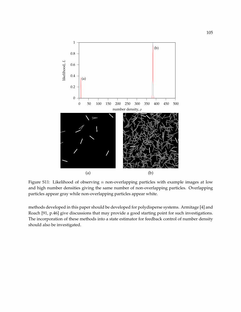
105

0

0.2

0.4

0.6

0.8

1

0 50 100 150 200 250 300 350 400 450 500

likel

ihoo

d,L

number density, ρ

(a)

(b)

(a) (b)

Figure S11: Likelihood of observing n non-overlapping particles with example images at lowand high number densities giving the same number of non-overlapping particles. Overlappingparticles appear gray while non-overlapping particles appear white.

methods developed in this paper should be developed for polydisperse systems. Armitage [4] andRoach [91, p.46] give discussions that may provide a good starting point for such investigations.The incorporation of these methods into a state estimator for feedback control of number densityshould also be investigated.

106

Chapter 9

Parameter Estimation Using ImagingData OR Feasibility of PSDreconstruction in finite time

107

Chapter 10

Conclusion10.1 Contributions

10.2 Future work

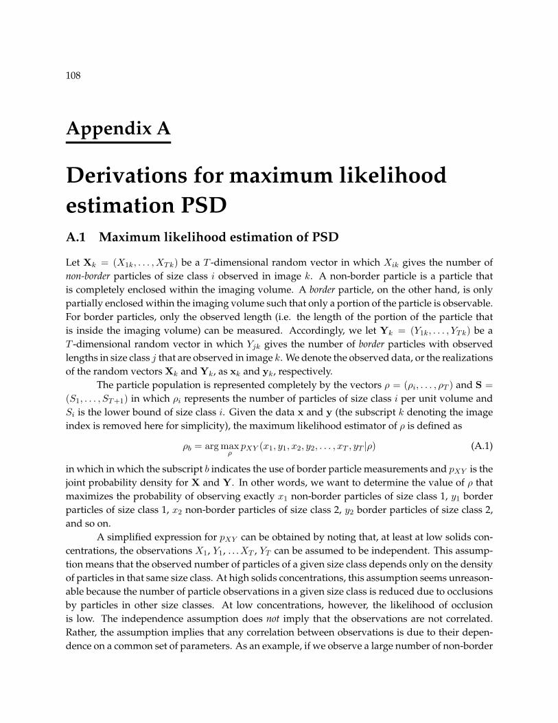
108

Appendix A

Derivations for maximum likelihoodestimation PSDA.1 Maximum likelihood estimation of PSD

Let Xk = (X1k, . . . , XTk) be a T -dimensional random vector in which Xik gives the number ofnon-border particles of size class i observed in image k. A non-border particle is a particle thatis completely enclosed within the imaging volume. A border particle, on the other hand, is onlypartially enclosed within the imaging volume such that only a portion of the particle is observable.For border particles, only the observed length (i.e. the length of the portion of the particle thatis inside the imaging volume) can be measured. Accordingly, we let Yk = (Y1k, . . . , YTk) be aT -dimensional random vector in which Yjk gives the number of border particles with observedlengths in size class j that are observed in image k. We denote the observed data, or the realizationsof the random vectors Xk and Yk, as xk and yk, respectively.

The particle population is represented completely by the vectors ρ = (ρi, . . . , ρT ) and S =(S1, . . . , ST+1) in which ρi represents the number of particles of size class i per unit volume andSi is the lower bound of size class i. Given the data x and y (the subscript k denoting the imageindex is removed here for simplicity), the maximum likelihood estimator of ρ is defined as

ρb = arg maxρ

pXY (x1, y1, x2, y2, . . . , xT , yT |ρ) (A.1)

in which in which the subscript b indicates the use of border particle measurements and pXY is thejoint probability density for X and Y. In other words, we want to determine the value of ρ thatmaximizes the probability of observing exactly x1 non-border particles of size class 1, y1 borderparticles of size class 1, x2 non-border particles of size class 2, y2 border particles of size class 2,and so on.

A simplified expression for pXY can be obtained by noting that, at least at low solids con-centrations, the observations X1, Y1, . . . XT , YT can be assumed to be independent. This assump-tion means that the observed number of particles of a given size class depends only on the densityof particles in that same size class. At high solids concentrations, this assumption seems unreason-able because the number of particle observations in a given size class is reduced due to occlusionsby particles in other size classes. At low concentrations, however, the likelihood of occlusionis low. The independence assumption does not imply that the observations are not correlated.Rather, the assumption implies that any correlation between observations is due to their depen-dence on a common set of parameters. As an example, if we observe a large number of non-border

109

particles, we would expect to also observe a large number of border particles. This correlation canbe explained by noting that the probability densities for both border and non-border observa-tions depend on a common parameter, namely, the density of particles. Given the independenceassumption, we express pXY as

pXY =T∏

i=1

pXi(xi|ρ)T∏

j=1

pYj (yj |ρ) (A.2)

in which pXi and pYj are the probability densities for the random variables Xi and Yj . UsingEquation (A.2), the estimator in Equation (A.1) can be reformulated as

ρb = arg minρ

T∑i=1

− log pXi(xi|ρ)−T∑

j=1

log pYj (yj |ρ) (A.3)

The probability densities pXi and pYj are derived in the following sections. These deriva-tions show that Xi ∼ Poisson(mXi), or that Xi has a Poisson distribution with parameter mXi =ρiαi, in which αi is a function of the field of view, depth of field, and the lower and upper boundsof size class i. Furthermore, Yj ∼ Poisson(mYj ), in which mYj =

∑Ti=1 ρiβij

A.2 Derivation of probability densities

The probability densities pXi and pYi in Equation (A.3) can be derived given the particle geom-etry and the spatial and orientational probability distributions. Here, we derive pXi and pYi forneedle-like particles assuming the particles are randomly, uniformly distributed, both in their 3-dimensional spatial location and in their orientation in the plane perpendicular to the optical axis.To simplify the discussion, we initially present the derivation assuming a 2-dimensional systemwith monodisperse, vertically-oriented particles. Later, we relax these assumptions and presentthe derivation for randomly-oriented, polydisperse particles in 3-dimensional space.

A.2.1 Non-border particles

Let S be a square domain in R2 with dimension B and area AS = B2. Let I be a rectangulardomain in R2 with horizontal and vertical dimensions a and b, respectively, and area AI = ab.Assume AI AS and I ∈ S. Let ntot be the total number of vertically-oriented particles withmidpoints randomly and uniformly distributed in S, and define ρ = ntot/AS as the density ofparticles per unit area. Let the length of all particles be l, with l < min (a, b), and define Anb as thearea of the domain in which particles are inside I but do not touch the border of I . Because theparticles are oriented vertically, it is easy to show that Anb = a(b − l), as depicted in Figure S1(a).Finally, let X be a random variable denoting the number of non-border particles appearing in I .Assuming the location of each particle in S is independent of the remaining particles’ locations,the probability that a specific particle will appear entirely within I is given by p = Anb/AS . Giventhe above assumptions, this probability is constant for all particles. The probability of observing x

110

l/2I

b

a

Anb

l/2l

S

a

l l

I

b

S

Ab

(a) (b)

Figure S1: Depiction of hypothetical system of vertically-oriented particles randomly and uni-formly distributed in space.

non-border particles in I is analogous to the probability of observing x successes in ntot Bernoullitrials in which the probability of success in each trial is p. Thus, X is a binomial random variablewith probability distribution

pX(x) =

(ntot

x

)px(1− p)ntot−x

Now, assume B →∞ while keeping ρ constant. Then ntot →∞ and p = Anb/AS = Anbρ/ntot → 0while Np = ρAnb remains constant. The limiting distribution of X is therefore Poisson

pX(x) =e−mX mx

X

x!, mX = ρAnb

To extend the analysis to polydisperse, randomly-oriented needles, we discretize the lengthscale into T size classes and let X = (X1, . . . , XT ) be a T -dimensional random vector in which Xi

gives the number of non-border particles of size class i observed in a single image. An orientation Θand length L are assigned to each particle, where Θ1,Θ2, . . . ,Θntot are i.i.d. with density functionpΘ(θ), θ ∈ [−π/2, π/2) and L1, L2, . . . , Lntot are i.i.d. with density function pL(l), l ∈ (0, inf). Θ andL are independent of each other and independent of the particle’s spatial location. We define S asthe T+1-dimensional vector of breaks between size classes. A particle of length l belongs to sizeclass i if Si ≤ l < Si+1. Let ∆i = Si+1 − Si. Our goal is to determine the probability that a particleof size class i will appear entirely inside the image I , given its density ρi. Following the approachused to solve the Buffon-Laplace needle problem [102, p. 4], Figure S2 shows geometrically thatfor a given orientation θ and length l, Anb(l, θ) can be calculated as

Anb(l, θ) =

(a− l cos θ)(b− l sin θ) 0 ≤ θ ≤ π/2(a− l cos θ)(b + l sin θ) −π/2 ≤ θ ≤ 0

(A.4)

111

l

Anb(l, θ)

a

b

θ

l/2 cos θ l/2 cos θ

l/2 sin θ

l/2 sin θ

Figure S2: Depiction of geometrical properties used to derive the non-border area functionAnb(l, θ).

The probability that a given particle in size class i will appear entirely within I is given by

pi =

∫ Si+1

Si

∫ π2

−π2

Anb(l, θ)pΘ(θ)pL(l)dθdl∫ Si+1

Si

∫ π2

−π2

ASpΘ(θ)pL(l)dθdl

(A.5)

Thus, the probability that a specific particle of size class i will appear entirely within the image isgiven by pi = αi/AS , where αi is the numerator in Equation (A.5). Following the same argumentsas above, we can show that for an infinitely large system, Xi is a Poisson random variable withparameter mXi = ρiαi.

Extending the analysis to three-dimensional space is trivial because we assume the parti-cles are oriented in the plane perpendicular to the camera’s optical axis and assume no interactionbetween particles. Thus, for a three-dimensional system, Xi is a Poisson random variable withparameter mXi = ρiαi, with αi = αid, in which d is the depth of field.

Assuming Θ is distributed uniformly and L is distributed uniformly across each size class,αi can be calculated as follows. Let ∆Si = Si+1 − Si, Smax =

√a2 + b2, ∆Si,max = Smax − Si, and

assume a > b. For Si+1 ≤ b,

αi =d

π∆Si

[13(S3

i+1 − S3i

)− (a + b)

(S2

i+1 − S2i

)+ abπ∆Si

]For b < Si, Si+1 ≤ a,

αi =d

π∆Si

[Si+1

(a√

S2i+1 − b2 + 2ab sin−

(b

Si+1

)− b

)· · ·

− Si

(a√

S2i − b2 + 2ab sin−

(b

Si

)+ b

)· · ·

+ab2 log

Si+1 +√

S2i+1 − b2

Si +√

S2i − b2

− a(S2

i+1 − S2i

)

112

For a ≤ Si, Si+1 ≤ Smax,

αi =d

π∆Si

Si+1

[a√

S2i+1 − b2 + b

√S2

i+1 − a2 + 2ab

(sin−

(b

Si+1

)− cos−

(a

Si+1

))]· · ·

− Si

[a√

S2i − b2 + b

√S2

i − a2 + 2ab

(sin−

(b

Si

)− cos−

(a

Si

))]· · ·

+ ab2 log

Si+1 +√

S2i+1 − b2

Si +√

S2i − b2

+ a2b log

Si+1 +√

S2i+1 − a2

Si +√

S2i − a2

· · ·−(a2 + b2)∆Si −

13(S3

i+1 − S3i

)For a ≤ Si ≤ Smax and Si+1 > Smax,

αi =d

π∆Si,max

Smax

[a√

S2max − b2 + b

√S2

max − a2 + 2ab

(sin−

(b

Smax

)− cos−

(a

Smax

))]· · ·

− Si

[a√

S2i − b2 + b

√S2

i − a2 + 2ab

(sin−

(b

Si

)− cos−

(a

Si

))]· · ·

+ ab2 log

Smax +√

S2max − b2

Si +√

S2i − b2

+ a2b log

Smax +√

S2max − a2

Si +√

S2i − a2

· · ·−(a2 + b2)∆Si,max −

13(S3

max − S3i

)

A.2.2 Border particles

As before, we simplify the discussion by first presenting the derivation of pYi for monodisperse,vertically-oriented particles. Let Y be a random variable denoting the total number of borderparticles appearing in I . Define Ab as the area of the domain in which particles touch the borderof I , as depicted in Figure S3(a). For the present system, Ab = 2al. The probability that a specificparticle will touch the border of I is given by p = Ab/AS . Following the same arguments as above,we can show that for an infinitely large system, Y is a Poisson random variable with parametermY = ρAb.

Now, assume we would like to incorporate additional information into our estimation bytaking into account not only the number of border particles, but also their observed lengths. Fora monodisperse population, these observed lengths can take on values anywhere between 0 andl. We therefore discretize the length scale on [0 l] and let j denote the size class corresponding tothe observed length. We define Yj as a random variable denoting the number of border particlesappearing in I with observed length in size class j. Figure S3(b) illustrates this approach fortwo size classes. In this figure, Ab1 is the area of the region in which particles produce observedlengths from 0 to l/2, corresponding to size class 1, while Ab2 is the area of the region in whichparticles produce observed lengths from l/2 to l, corresponding to size class 2. The probability

113

a

l l

I

b

S

Ab

a

l

b

S

Ab2

l

Ab1

I

S

Ab1 Ab2

(a) (b) (c)

Figure S3: Depiction of hypothetical system of vertically-oriented particles randomly and uni-formly distributed in space.

that a specific particle will touch the border of I and produce an observed length in size class j isp = Abj

/AS . Thus, Yj is a Poisson random variable with parameter mYj = ρAbj.

In Figure S3(b), Ab1 = Ab2 . This equality between the areas of different observed length sizeclasses does not hold in general, however, as illustrated in Figure S3(c). In this figure, we assumeall particles are oriented diagonally, at 45 degrees from the horizontal, and the figure illustratesthat Ab1 > Ab2 . Hence, in general, border particles are more likely to result in observed lengths inthe lower size classes.

To extend the analysis to polydisperse systems with random orientation, we define a newrandom variable Yij that gives the number of particles in size class i that intersect the image bor-der, producing an observed length in size class j. Given that the size class of each border particleis unknown, we define the random variable Yj as the total number of border particles produc-ing observed lengths in size class j, noting that Yj =

∑i Yij . Our approach is to determine the

probability density for Yij for all i and to use these densities to derive the probability density forYj .

We define the function Abj(l, θ) as the area of the region in which a particle of length l and

orientation θ produces an observed length corresponding to size class j. To calculate Abj(l, θ), it

is convenient to define an area function A(l, θ, l) as the area of the region in which particles oflength l and orientation θ either intersect or are enclosed within the image boundary and producean observed length greater than or equal to l. A(l, θ, l) can be calculated using the geometricrelationships shown in Figure S4: In this figure, the thick-lined, outer rectangle is the image region,and the inner rectangle is the region inside which a particle with length l and orientation θ willbe entirely enclosed within the image boundary, thus producing an observed length of exactlyl. A particle with its midpoint along the perimeter of the outermost hexagon would touch theimage boundary but give an observed length of 0. A particle with its midpoint anywhere insidethe innermost hexagon will produce an observed length greater than or equal to l. Using the

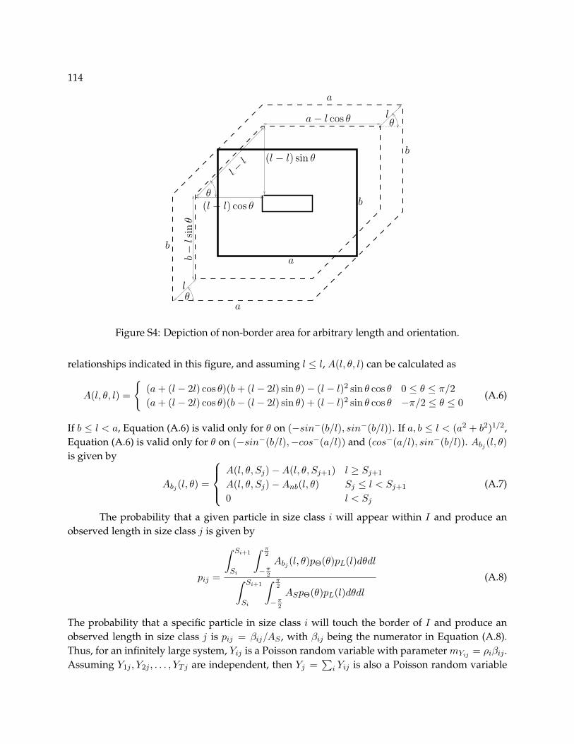
114

θl

a

b−

lsin

θ

b

(l − l) sin θ

a− l cos θ

a

lθ

b

b

a

(l − l) cos θ

l −l

θ

Figure S4: Depiction of non-border area for arbitrary length and orientation.

relationships indicated in this figure, and assuming l ≤ l, A(l, θ, l) can be calculated as

A(l, θ, l) =

(a + (l − 2l) cos θ)(b + (l − 2l) sin θ)− (l − l)2 sin θ cos θ 0 ≤ θ ≤ π/2(a + (l − 2l) cos θ)(b− (l − 2l) sin θ) + (l − l)2 sin θ cos θ −π/2 ≤ θ ≤ 0

(A.6)

If b ≤ l < a, Equation (A.6) is valid only for θ on (−sin−(b/l), sin−(b/l)). If a, b ≤ l < (a2 + b2)1/2,Equation (A.6) is valid only for θ on (−sin−(b/l),−cos−(a/l)) and (cos−(a/l), sin−(b/l)). Abj

(l, θ)is given by

Abj(l, θ) =

A(l, θ, Sj)−A(l, θ, Sj+1) l ≥ Sj+1

A(l, θ, Sj)−Anb(l, θ) Sj ≤ l < Sj+1

0 l < Sj

(A.7)

The probability that a given particle in size class i will appear within I and produce anobserved length in size class j is given by

pij =

∫ Si+1

Si

∫ π2

−π2

Abj(l, θ)pΘ(θ)pL(l)dθdl∫ Si+1

Si

∫ π2

−π2

ASpΘ(θ)pL(l)dθdl

(A.8)

The probability that a specific particle in size class i will touch the border of I and produce anobserved length in size class j is pij = βij/AS , with βij being the numerator in Equation (A.8).Thus, for an infinitely large system, Yij is a Poisson random variable with parameter mYij = ρiβij .Assuming Y1j , Y2j , . . . , YTj are independent, then Yj =

∑i Yij is also a Poisson random variable

115

with parameter mYj =∑

i ρiβij [12, p.440]. As in the non-border case, the analysis is extendedto three-dimensional space assuming the particles are oriented in the plane perpendicular to thecamera’s optical axis and that the particles do not interact. Thus, for a three-dimensional system,Yj is a Poisson random variable with parameter mYj =

∑i ρiβij , with βij = βijd.

Assuming Θ is distributed uniformly and L is distributed uniformly across each size class,βij is calculated as follows. Let the length scale discretization be the same for both border andnon-border particles. As before, let ∆Si = Si+1 − Si, Smax =

√a2 + b2, ∆Si,max = Smax − Si, and

assume a > b. Then βij is given by

βij =

A(i, Sj)−A(i, Sj+1) i > j

A(i, Sj)− αi i = j

0 i < j

(A.9)

in which A(i, S) is calculated as

A(i, S) =d

π∆Si

[∆Si

(2abγ1 − 4bSγ2 − 4aSγ3 + 3S2γ4

)+(S2

i+1 − S2i

)(bγ2 + aγ3 − Sγ4)

]

γ1 =

π/2 S < b

sin− (b/S) b < S < a

sin− (b/S)− cos− (a/S) a < S < Smax

sin− (b/Smax)− cos− (a/Smax) S > Smax

γ2 =

1 S < b

b/S b < S < a(b−

√S2 − a2

)/S a < S < Smax(

b−√

S2max − a2

)/Smax S > Smax

γ3 =

1 S < b

1−√

S2 − b2/S b < S < a(a−

√S2 − b2

)/S a < S < Smax(

a−√

S2max − b2

)/Smax S > Smax

γ4 =

1 S < b

b2/S2 b < S < a

(a2 + b2 − S2)/S2 a < S < Smax

(a2 + b2 − S2max)/S2

max S > Smax

A.3 Validation of Marginal Densities

To ensure the correctness of the probability densities derived in the previous section, four differentMonte Carlo simulations were carried out in which artificial images of particulate populationswere generated. Figure S5 shows example images generated for each simulation. Each of these

116

images has a horizontal image dimension of a=480 pixels and a vertical dimension of b=480 pixels.The first row displays four simulated images for monodisperse particles of length 0.5a with Nc=25crystals per image. The second row shows images of particles uniformly distributed on [0.1a 0.9a]with Nc=25. The third row shows images of particles normally-distributed with µ = 0.5a andσ = 0.4a/3 with Nc=25, and the fourth row shows example images for simulations of particlesuniformly-distributed on [0.1a 2.0a] with Nc=15. For each simulation, 20,000 artificial imageswere generated. Based on the observations in these 20,000 images, a histogram was generatedfor each size class giving the frequency of observations for both border and non-border particles.These histograms are compared with the theoretical marginal densities in Figures S6– S13.

117

Figure S5: Example images for simulations of various particle populations. Row 1: monodis-perse particles of length 0.5a, Nc=25. Row 2: particles uniformly distributed on [0.1a 0.9a]. Row3: particles normally-distributed with µ = 0.5a and σ = 0.4a/3 with Nc=25. Row 4: particlesuniformly-distributed on [0.1a 2.0a], Nc=15.

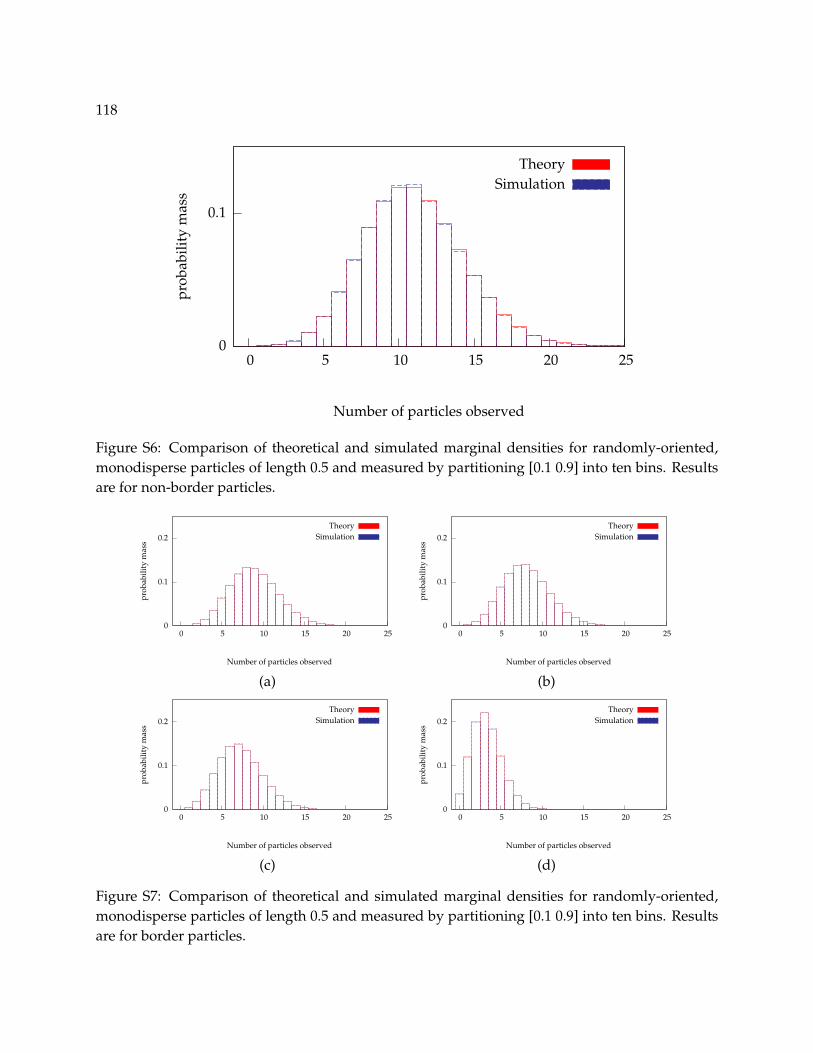
118

0

0.1

0 5 10 15 20 25

prob

abili

tym

ass

Number of particles observed

TheorySimulation

Figure S6: Comparison of theoretical and simulated marginal densities for randomly-oriented,monodisperse particles of length 0.5 and measured by partitioning [0.1 0.9] into ten bins. Resultsare for non-border particles.

0

0.1

0.2

0 5 10 15 20 25

prob

abili

tym

ass


TheorySimulation

0

0.1

0.2

0 5 10 15 20 25

prob

abili

tym

ass


TheorySimulation

(a) (b)

0

0.1

0.2

0 5 10 15 20 25

prob

abili

tym

ass


TheorySimulation

0

0.1

0.2

0 5 10 15 20 25

prob

abili

tym

ass


TheorySimulation

(c) (d)

Figure S7: Comparison of theoretical and simulated marginal densities for randomly-oriented,monodisperse particles of length 0.5 and measured by partitioning [0.1 0.9] into ten bins. Resultsare for border particles.

119

0

0.9

0 2 4 6 8 10 12 14 16

prob

abili

tym

ass


TheorySimulation

0

0.9

0 2 4 6 8 10 12 14 16

prob

abili

tym

ass


TheorySimulation

0

0.9

0 2 4 6 8 10 12 14 16

prob

abili

tym

ass


TheorySimulation

0

0.9

0 2 4 6 8 10 12 14 16pr

obab

ility

mas

s


TheorySimulation

0

0.9

0 2 4 6 8 10 12 14 16

prob

abili

tym

ass


TheorySimulation

0

0.9

0 2 4 6 8 10 12 14 16

prob

abili

tym

ass


TheorySimulation

0

0.9

0 2 4 6 8 10 12 14 16

prob

abili

tym

ass


TheorySimulation

0

0.9

0 2 4 6 8 10 12 14 16

prob

abili

tym

ass


TheorySimulation

0

0.9

0 2 4 6 8 10 12 14 16

prob

abili

tym

ass


TheorySimulation

0

0.9

0 2 4 6 8 10 12 14 16

prob

abili

tym

ass


TheorySimulation

Figure S8: Comparison of theoretical and simulated marginal densities for randomly-orientedparticles distributed uniformly on [0.1 0.9] and measured by partitioning [0.1 0.9] into ten bins.Results are for non-border particles.

120

0

0.9

0 2 4 6 8 10 12 14 16

prob

abili

tym

ass


TheorySimulation

0

0.9

0 2 4 6 8 10 12 14 16

prob

abili

tym

ass


TheorySimulation

0

0.9

0 2 4 6 8 10 12 14 16

prob

abili

tym

ass


TheorySimulation

0

0.9

0 2 4 6 8 10 12 14 16pr

obab

ility

mas

s


TheorySimulation

0

0.9

0 2 4 6 8 10 12 14 16

prob

abili

tym

ass


TheorySimulation

0

0.9

0 2 4 6 8 10 12 14 16

prob

abili

tym

ass


TheorySimulation

0

0.9

0 2 4 6 8 10 12 14 16

prob

abili

tym

ass


TheorySimulation

0

0.9

0 2 4 6 8 10 12 14 16

prob

abili

tym

ass


TheorySimulation

0

0.9

0 2 4 6 8 10 12 14 16

prob

abili

tym

ass


TheorySimulation

0

0.9

0 2 4 6 8 10 12 14 16

prob

abili

tym

ass


TheorySimulation

Figure S9: Comparison of theoretical and simulated marginal densities for randomly-orientedparticles distributed uniformly on [0.1 0.9] and measured by partitioning [0.1 0.9] into ten bins.Results are for border particles.

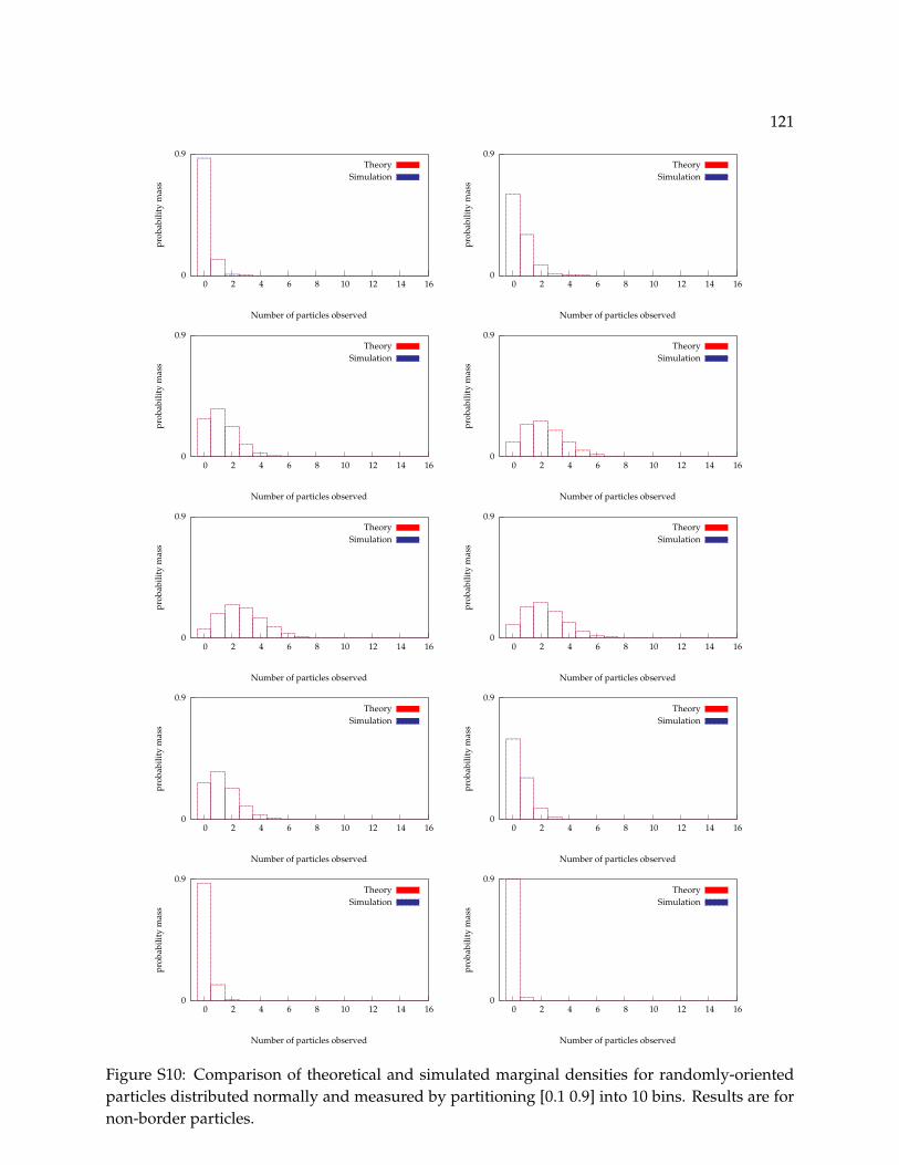
121

0

0.9

0 2 4 6 8 10 12 14 16

prob

abili

tym

ass


TheorySimulation

0

0.9

0 2 4 6 8 10 12 14 16

prob

abili

tym

ass


TheorySimulation

0

0.9

0 2 4 6 8 10 12 14 16

prob

abili

tym

ass


TheorySimulation

0

0.9

0 2 4 6 8 10 12 14 16pr

obab

ility

mas

s


TheorySimulation

0

0.9

0 2 4 6 8 10 12 14 16

prob

abili

tym

ass


TheorySimulation

0

0.9

0 2 4 6 8 10 12 14 16

prob

abili

tym

ass


TheorySimulation

0

0.9

0 2 4 6 8 10 12 14 16

prob

abili

tym

ass


TheorySimulation

0

0.9

0 2 4 6 8 10 12 14 16

prob

abili

tym

ass


TheorySimulation

0

0.9

0 2 4 6 8 10 12 14 16

prob

abili

tym

ass


TheorySimulation

0

0.9

0 2 4 6 8 10 12 14 16

prob

abili

tym

ass


TheorySimulation

Figure S10: Comparison of theoretical and simulated marginal densities for randomly-orientedparticles distributed normally and measured by partitioning [0.1 0.9] into 10 bins. Results are fornon-border particles.

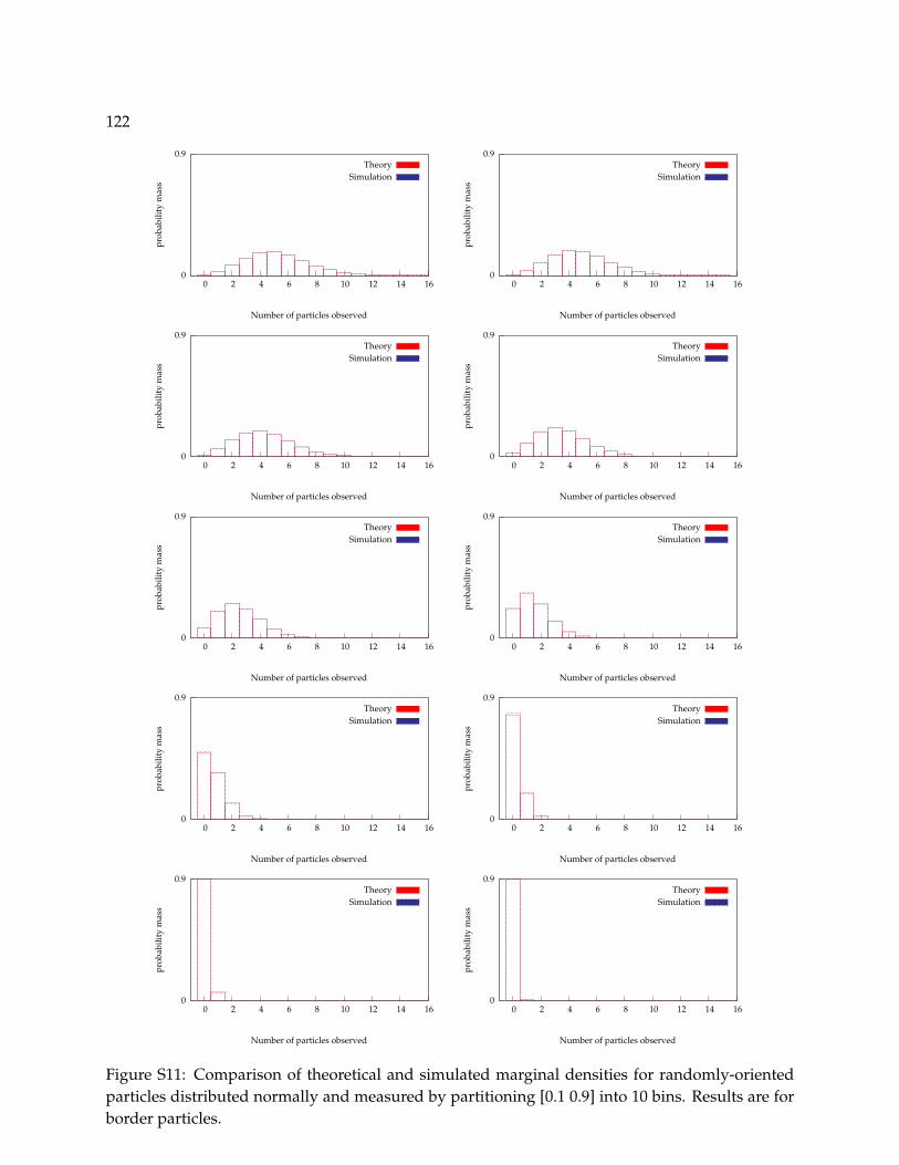
122

0

0.9

0 2 4 6 8 10 12 14 16

prob

abili

tym

ass


TheorySimulation

0

0.9

0 2 4 6 8 10 12 14 16

prob

abili

tym

ass


TheorySimulation

0

0.9

0 2 4 6 8 10 12 14 16

prob

abili

tym

ass


TheorySimulation

0

0.9

0 2 4 6 8 10 12 14 16pr

obab

ility

mas

s


TheorySimulation

0

0.9

0 2 4 6 8 10 12 14 16

prob

abili

tym

ass


TheorySimulation

0

0.9

0 2 4 6 8 10 12 14 16

prob

abili

tym

ass


TheorySimulation

0

0.9

0 2 4 6 8 10 12 14 16

prob

abili

tym

ass


TheorySimulation

0

0.9

0 2 4 6 8 10 12 14 16

prob

abili

tym

ass


TheorySimulation

0

0.9

0 2 4 6 8 10 12 14 16

prob

abili

tym

ass


TheorySimulation

0

0.9

0 2 4 6 8 10 12 14 16

prob

abili

tym

ass


TheorySimulation

Figure S11: Comparison of theoretical and simulated marginal densities for randomly-orientedparticles distributed normally and measured by partitioning [0.1 0.9] into 10 bins. Results are forborder particles.

123

0

0.9

0 2 4 6 8 10 12 14 16

prob

abili

tym

ass


TheorySimulation

0

0.9

0 2 4 6 8 10 12 14 16

prob

abili

tym

ass


TheorySimulation

0

0.9

0 2 4 6 8 10 12 14 16

prob

abili

tym

ass


TheorySimulation

0

0.9

0 2 4 6 8 10 12 14 16pr

obab

ility

mas

s


TheorySimulation

0

0.9

0 2 4 6 8 10 12 14 16

prob

abili

tym

ass


TheorySimulation

0

0.9

0 2 4 6 8 10 12 14 16

prob

abili

tym

ass


TheorySimulation

0

0.9

0 2 4 6 8 10 12 14 16

prob

abili

tym

ass


TheorySimulation

0

0.9

0 2 4 6 8 10 12 14 16

prob

abili

tym

ass


TheorySimulation

0

0.9

0 2 4 6 8 10 12 14 16

prob

abili

tym

ass


TheorySimulation

0

0.9

0 2 4 6 8 10 12 14 16

prob

abili

tym

ass


TheorySimulation

Figure S12: Comparison of theoretical and simulated marginal densities for randomly-orientedparticles distributed uniformly on [0.4 2.0] and measured by partitioning [0.4 1.0] into 9 bins witha 10th bin spanning [1.0

√2]. Results are for non-border particles.

124

0

0.9

0 2 4 6 8 10 12 14 16

prob

abili

tym

ass


TheorySimulation

0

0.9

0 2 4 6 8 10 12 14 16

prob

abili

tym

ass


TheorySimulation

0

0.9

0 2 4 6 8 10 12 14 16

prob

abili

tym

ass


TheorySimulation

0

0.9

0 2 4 6 8 10 12 14 16pr

obab

ility

mas

s


TheorySimulation

0

0.9

0 2 4 6 8 10 12 14 16

prob

abili

tym

ass


TheorySimulation

0

0.9

0 2 4 6 8 10 12 14 16

prob

abili

tym

ass


TheorySimulation

0

0.9

0 2 4 6 8 10 12 14 16

prob

abili

tym

ass


TheorySimulation

0

0.9

0 2 4 6 8 10 12 14 16

prob

abili

tym

ass


TheorySimulation

0

0.9

0 2 4 6 8 10 12 14 16

prob

abili

tym

ass


TheorySimulation

0

0.9

0 2 4 6 8 10 12 14 16

prob

abili

tym

ass


TheorySimulation

Figure S13: Comparison of theoretical and simulated marginal densities for randomly-orientedparticles distributed uniformly on [0.4 2.0] and measured by partitioning [0.4 1.0] into 9 bins witha 10th bin spanning [1.0

√2]. Results are for border particles.

125

Bibliography[1] Stochastic Geometry and Its Applications. John Wiley & Sons, Chichester, 1987.

[2] P. Agarwal and K. A. Berglund. In situ monitoring of calcium carbonate polymorphs during batch crystallizationin the presence of polymeric additives using Raman spectroscopy. Crystal Growth and Design, 3(6):941–946, 2003.

[3] T. Allen. Powder Sampling and Particle Size Determination. Elsevier, 2003.

[4] P. Armitage. An overlap problem arising in particle counting. Biometrika, 36(3/4):257–266, December 1949.

[5] A. J. Baddeley. Stochastic Geometry Likelihood and Computation, chapter Spatial sampling and censoring, pages37–78. Chapman and Hall/CRC, Boca Raton, FL, 1999.

[6] A. J. Baddeley. Stochastic Geometry Likelihood and Computation, chapter A crash course in stochastic geometry,pages 1–35. Chapman and Hall/CRC, Boca Raton, FL, 1999.

[7] P. Barrett. Selecting in-process particle-size analyzers. Chemical Engineering Progress, 99(8):26–32, August 2003.

[8] P. Barrett and B. Glennon. In-line FBRM monitoring of particle size in dilute agitated suspensions. Particle andParticle Systems Characterization, 16(5):207–211, 1999.

[9] P. Barrett and B. Glennon. Characterizing the metastable zone width and solubility curve using Lasentec FBRMand PVM. Chemical Engineering Research and Design, 80(A7):799–805, 2002.

[10] J. Bauer, S. Spanton, R. Henry, J. Quick, W. Dziki, W. Porter, and J. Morris. Ritonavir: An extraordinary exampleof conformational polymorphism. Pharmaceutical Research, 18(6):859–866, 2001.

[11] M. Birch, S. J. Fussell, P. D. Higginson, N. McDowall, and I. Marziano. Towards a PAT-based strategy for crystal-lization development. Organic Process Research & Development, 9(3):360–364, 2005.

[12] Y. M. M. Bishop, S. E. Fienberg, and P. W. Holland. Discrete Multivariate Analysis: Theory and Practice. The MITPress, Cambridge, Massachusetts, 1975.

[13] N. Blagden, R. Davey, R. Rowe, and R. Roberts. Disappearing polymorphs and the role of reaction by-products:The case of sulphathiazole. International Journal of Pharmaceutics, 172(1–2):169–177, 1998.

[14] S. Boerrigter, G. Josten, J. van de Streek, F. Hollander, J.Los, H. Cuppen, P. Bennema, and H. Meekes. MONTY:Monte Carlo crystal growth on any crystal structure in any crystallographic orientation; application to fats. Jour-nal of Physical Chemistry A, 108(27):5894–5902, 2004.

[15] R. D. Braatz. Advanced control of crystallization processes. Annual Reviews in Control, 26:87–99, 2002.

[16] R. D. Braatz and S. Hasebe. Particle size and shape control in crystallization processes. In Chemical ProcessControl—CPC 6, pages 307–327, Tucson, Arizona, January 2001.

[17] J. B. Burns, A. R. Hanson, and E. M. Riseman. Extracting straight lines. IEEE Transactions on Pattern Analysis andMachine Intelligence, 8(4):425–455, July 1986.

126

[18] J. Calderon De Anda, X. Wang, X. Lai, and K. Roberts. Classifying organic crystals via in-process image analysisand the use of monitoring charts to follow polymorphic and morphological changes. Journal of Process Control,15(7):785–797, 2005.

[19] J. Calderon De Anda, X. Wang, and K. Roberts. Multi-scale segmentation image analysis for the in-processmonitoring of particle shape with batch crystallizers. Chemical Engineering Science, 60:1053–1065, 2005.

[20] S. Christy and R. Horaud. Iterative pose computation from line correspondences. Computer Vision and ImageUnderstanding, 73(1):137–144, January 1999.

[21] S. H. Chung, D. L. Ma, and R. D. Braatz. Optimal seeding in batch crystallization. The Canadian Journal of ChemicalEngineering, 77(3):590–596, 1999.

[22] G. Clydesdale, R. Docherty, and K. J. Roberts. HABIT—a program for predicting the morphology of molecularcrystals. Computer Physics Communications, 64(2):311–328, 1991.

[23] W. W. Daniel. Applied Nonparametric Statistics. Houghton Mifflin Company, Boston, MA, 1978.

[24] S. Datta and D. J. W. Grant. Crystal structure of drugs: Advances in determination, prediction and engineering.Nature Reviews Drug Discovery, 3(1):42–57, January 2004.

[25] C. Deeley, R. Spragg, and T. Threlfall. A comparison of Fourier-Transform Infrared and Near-Infrared Fourier-Transform Raman-spectroscopy for quantitative measurements — An application in polymorphism. Spectrochim-ica Acta A, 47(9–10):1217–1223, 1991.

[26] M. Dhome, M. Richetin, J.-T. Lapreste, and G. Rives. Determination of the attitude of 3-D objects from a singleperspective view. IEEE Transactions on Pattern Analysis and Machine Intelligence, 11(12):1265–1278, December 1989.

[27] N. Doki, H. Seki, K. Takano, H. Asatani, M. Yokota, and N. Kubota. Process control of seeded batch coolingcrystallization of the metastable α-form glycine using an in-situ ATR-FTIR spectrometer and an in-situ FBRMparticle counter. Crystal Growth and Design, 4(5):949–953, 2004.

[28] W. Doyle. Technical note AN-923. A user’s guide to: spectroscopic analysis for industrial applications. Technicalreport, Axiom Analytical, Inc., Irvine, CA, January 2005.

[29] D. D. Dunuwila and K. A. Berglund. ATR FTIR spectroscopy for in situ measurement of supersaturation. Journalof Crystal Growth, 179(1–2):185–193, 1997.

[30] D. D. Dunuwila, L. B. Carroll II, and K. A. Berglund. An investigation of the applicability of attenuated total re-flection infrared spectroscopy for measurement of solubility and supersaturation of aqueous citric acid solutions.Journal of Crystal Growth, 137(3–4):561–568, 1994.

[31] A. Etemadi, J.-P. Schmidt, G. Matas, J. Illingworth, and J. Kittler. Low-level grouping of straight line segments.In Proceedings of the British Machine Vision Conference, 1991.

[32] J. A. Falcon and K. A. Berglund. Monitoring of antisolvent addition crystallization with Raman spectroscopy.Crystal Growth and Design, 3(6):947–952, 2003.

[33] L. Feng and K. A. Berglund. ATR-FTIR for determining optimal cooling curves for batch crystallization of succinicacid. Crystal Growth and Design, 2(5):449–452, 2002.

[34] G. Fevotte. New perspectives for the on-line monitoring of pharmaceutical crystallization processes using in situinfrared spectroscopy. International Journal of Pharmaceutics, 241(2):263–278, 2002.

[35] G. Fevotte, J. Calas, F. Puel, and C. Hoff. Applications of NIR spectroscopy to monitoring and analyzing the solidstate during industrial crystallization processes. International Journal of Pharmaceutics, 273(1–2):159–169, 2004.

127

[36] B. A. Finlayson. Nonlinear Analysis in Chemical Engineering. McGraw-Hill, New York, 1980.

[37] D. A. Forsyth and J. Ponce. Computer Vision: A Modern Approach. Prentice Hall series in artificial intelligence.Prentice Hall, New Jersey, 2003.

[38] M. Fujiwara, P. S. Chow, D. L. Ma, and R. D. Braatz. Paracetamol crystallization using laser backscattering andATR-FTIR spectroscopy: Metastability, agglomeration, and control. Crystal Growth and Design, 2(5):363–370, 2002.

[39] L. Gardini, A. Servida, M. Morbidelli, and S. Carra. Use of orthogonal collocation on finite elements with movingboundaries for fixed bed catalytic reactor simulation. Computers & Chemical Engineering, 9(1):1–17, 1985.

[40] G. H. Givens and J. A. Hoeting. Computational Statistics. Wiley Series in Probability and Statistics. John Wiley &Sons, New Jersey, 2005.

[41] R. C. Gonzalez and R. E. Woods. Digital Image Processing. Prentice Hall, second edition, 2002.

[42] D. A. Green. Particle formation and morphology control. DuPont Magazine, College Report supplement, Novem-ber/December 1988.

[43] W. Grimson and D. Huttenlocher. On the verification of hypothesized matches in model-based recognition. IEEETransactions on Pattern Analysis and Machine Intelligence, 13(12):1201–1213, 1989.

[44] H. Gron, A. Borissova, and K. Roberts. In-process ATR-FTIR spectroscopy for closed-loop supersaturation controlof a batch crystallizer producing monosodium glutamate crystals of defined size. Industrial and EngineeringChemistry Research, 42(1):198–206, 2003.

[45] P. Hall. Correcting segment counts for edge effects when estimating intensity. Biometrika, 72(2):459–63, 1985.

[46] R. W. Hartel. Crystallization in foods. In A. S. Myerson, editor, Handbook of industrial crystallization, pages 287–304.Butterworth-Heinemann, USA, 2nd edition, 2002.

[47] M. Honkanen, P. Saarenrinne, T. Stoor, and J. Niinimaki. Recognition of highly overlapping ellipse-like bubbleimages. Measurement Science and Technology, 16(9):1760–1770, 2005.

[48] R. Horaud, B. Conio, O. Leboulleux, and B. Lacolle. An analytic solution for the perspective 4-point problem.Computer Vision, Graphics, and Image Processing, 47:33–44, 1989.

[49] Y. Hu, J. K. Liang, A. S. Myerson, and L. S. Taylor. Crystallization monitoring by Raman spectroscopy: Simul-taneous measurement of desupersaturation profile and polymorphic form in flufenamic acid systems. Industrialand Engineering Chemistry Research, 44(5):1233–1240, 2005.

[50] E. J. Hukkanen and R. D. Braatz. Measurement of particle size distribution in suspension polymerization usingin situ laser backscattering. Sensors and Actuators B, 96:451–459, 2003.

[51] D. P. Huttenlocher. Recognition by alignment. In A. K. Jain and P. J. Flynn, editors, Three-dimensional objectrecognition systems, Advances in image communication, pages 311–326. Elsevier, Amsterdam, 1993.

[52] D. P. Huttenlocher and S. Ullman. Recognizing solid objects by alignment with an image. International Journal ofComputer Vision, 5(2):195–212, 1990.

[53] J.-H. Jang and K.-S. Hong. Fast line segment grouping method for finding globally more favorable line segments.Pattern Recognition, 35:2235–2247, 2002.

[54] P. Kahn, L. Kitchen, and E. Riseman. A fast line finder for vision-guided robot navigation. IEEE Transactions onPattern Analysis and Machine Intelligence, 12(11):1098–1102, November 1990.

128

[55] E. N. Kaufman and T. C. Scott. In situ visualization of coal particle distribution in a liquid fluidized bed usingfluorescence microscopy. Powder Technology, 78:239–246, 1994.

[56] A. Kellerer. On the number of clumps resulting from the overlap of randomly placed figures in a plane. Journalof Applied Probability, 20(1):126–135, 1983.

[57] C. Lantuejoul. Computation of the histograms of the number of edges and neighbours of cells in a tessellation. InR. Miles and J. Serra, editors, Geometrical Probability and Biological Structures: Buffon’s 200th Anniversary, number 23in Lecture Notes in Biomathematics, pages 323–329, Berlin-Heidelberg-New York, 1978. Springer-Verlag.

[58] P. A. Larsen and J. B. Rawlings. Derivations for maximum likelihood estimation of particle size distribution usingin situ video imaging. Technical Report 2007-01, TWMCC, Available at http://www.che.utexas.edu/twmcc/,March 2007.

[59] P. A. Larsen, J. B. Rawlings, and N. J. Ferrier. An algorithm for analyzing noisy, in situ images of high-aspect-aspect ratio crystals to monitor particle size distribution. Chemical Engineering Science, 61(16):5236–5248, 2006.

[60] P. A. Larsen, J. B. Rawlings, and N. J. Ferrier. Model-based object recognition to measure crystal size and shapedistributions from in situ video images. Chemical Engineering Science, 62:1430–1441, 2007.

[61] G. Laslett. The survival curve under monotone density constraints with application to two-dimensional linesegment processes. Biometrika, 69(1):153–160, 1982.

[62] F. Lewiner, J. P. Klein, F. Puel, and G. Fevotte. On-line ATR FTIR measurement of supersaturation during solutioncrystallization processes. Calibration and applications on three solute/solvent systems. Chemical EngineeringScience, 56(6):2069–2084, 2001.

[63] M. Li and D. Wilkinson. Determination of non-spherical particle size distribution from chord length measure-ments. Part 1: Theoretical analysis. Chemical Engineering Science, 60(12):3251–3265, 2005.

[64] V. Liotta and V. Sabesan. Monitoring and feedback control of supersaturation using ATR-FTIR to produce anactive pharmaceutical ingredient of a desired crystal size. Organic Process Research & Development, 8(3):488–494,2004.

[65] D. G. Lowe. Three-dimensional object recognition from single two-dimensional images. Artificial Intelligence,31(3):355–395, 1987.

[66] D. G. Lowe. Fitting parameterized three-dimensional models to images. IEEE Transactions on Pattern Analysis andMachine Intelligence, 13(5):441–450, 1991.

[67] Z. Ma and G. Guiochon. Application of orthogonal collocation on finite elements in the simulation of non-linearchromatography. Computers & Chemical Engineering, 15(6):415–426, 1991.

[68] C. Mack. The expected number of clumps when convex laminae are placed at random and with random orien-tation on a plane area. Proceedings of the Cambridge Philosophical Society, 50:581–585, 1954.

[69] C. Mack. On clumps formed when convex laminae or bodies are placed at random in two or three dimensions.Proceedings of the Cambridge Philosophical Society, 52:246–256, 1956.

[70] D. L. Marchisio, R. D. Vigil, and R. O. Fox. Quadrature method of moments for aggregation–breakage processes.Journal of Colloid and Interface Science, 258(2):322–334, 2003.

[71] F. J. Massey. The Kolmogorov-Smirnov test for goodness of fit. Journal of the Americal Statistical Association,46(253):68–78, March 1951.

129

[72] R. Miles. Stochastic Geometry, chapter On the elimination of edge effects in planar sampling, pages 228–247. JohnWiley & Sons, 1974.

[73] Milken Institute. Biopharmaceutical industry contributions to state and U.S. economies. Available atwww.milkeninstitute.org, 2004.

[74] S. M. Miller and J. B. Rawlings. Model identification and control strategies for batch cooling crystallizers. AIChEJournal, 40(8):1312–1327, August 1994.

[75] C. A. Mitchell, L. Yu, and M. D. Ward. Selective nucleation and discovery of organic polymorphs through epitaxywith single crystal substrates. Journal of the American Chemical Society, 123(44):10830–10839, 2001.

[76] S. Motz, S. Mannal, and E.-D. Gilles. Integral approximation—an approach to reduced models for particulateprocesses. Chemical Engineering Science, 59(5):987–1000, 2004.

[77] M. Naito, O. Hayakawa, K. Nakahira, H. Mori, and J. Tsubaki. Effect of particle shape on the particle sizedistribution measured with commercial equipment. Powder Technology, 100:52–60, 1998.

[78] T. Norris, P. K. Aldridge, and S. S. Sekulic. Determination of end-points for polymorph conversions of crystallineorganic compounds using on-line near-infrared spectroscopy. The Analyst, 122(6):549–552, 1997.

[79] L. E. O’Brien, P. Timmins, A. C. Williams, and P. York. Use of in situ FT-Raman spectroscopy to study the kineticsof the transformation of carbamazepine polymorphs. Journal of Pharmaceutical and Biomedical Analysis, 36(2):335–340, 2004.

[80] T. Ono, J. ter Horst, and P. Jansens. Quantitative measurement of the polymorphic transformation of L-glutamicacid using in-situ Raman spectroscopy. Crystal Growth and Design, 4(3):465–469, 2004.

[81] B. O’Sullivan, P. Barrett, G. Hsiao, A. Carr, and B. Glennon. In situ monitoring of polymorphic transitions. OrganicProcess Research & Development, 7(6):977–982, 2003.

[82] D. B. Patience. Crystal Engineering Through Particle Size and Shape Monitoring, Modeling, and Control. PhD thesis,University of Wisconsin–Madison, 2002.

[83] D. B. Patience, P. C. Dell’Orco, and J. B. Rawlings. Optimal operation of a seeded pharmaceutical crystallizationwith growth-dependent dispersion. Organic Process Research & Development, 8(4):609–615, 2004.

[84] D. B. Patience and J. B. Rawlings. Particle-shape monitoring and control in crystallization processes. AIChEJournal, 47(9):2125–2130, 2001.

[85] L. Petzold. Differential/algebraic equations are not ODE’s. SIAM Journal on Scientific and Statistical Computing,3(3):367–384, September 1982.

[86] M. Pons, H. Vivier, K. Belaroui, B. Bernard-Michel, F. Cordier, D. Oulhana, and J. Dodds. Particle morphology:from visualization to measurement. Powder Technology, 103:44–57, 1999.

[87] S. L. Price. The computational prediction of pharmaceutical crystal structures and polymorphism. Advanced DrugDelivery Reviews, 56(3):301–319, February 2004.

[88] F. Puel, P. Marchal, and J. Klein. Habit transient analysis in industrial crystallization using two dimensionalcrystal sizing technique. Chemical Engineering Research and Design, 75(A2):193–205, 1997.

[89] J. B. Rawlings, S. M. Miller, and W. R. Witkowski. Model identification and control of solution crystallizationprocesses: A review. Industrial and Engineering Chemistry Research, 32(7):1275–1296, July 1993.

130

[90] J. B. Rawlings, C. W. Sink, and S. M. Miller. Control of crystallization processes. In A. S. Myerson, editor, Handbookof industrial crystallization, pages 201–230. Butterworth-Heinemann, USA, 2nd edition, 2002.

[91] S. Roach. The Theory of Random Clumping. Methuen’s monographs on applied probability and statistics. Methuen& Company, London, 1968.

[92] S. Rohani and G. Zhang. On-line optimal control of a seeded batch cooling crystallizer. Chemical EngineeringScience, 58(9):1887–1896, 2003.

[93] A. L. Rohl. Computer prediction of crystal morphology. Current Opinion in Solid State & Material Science, 7(1):21–26, 2003.

[94] A. Ruf, J. Worlitschek, and M. Mazzotti. Modeling and experimental analysis of PSD measurements throughFBRM. Particle and Particle Systems Characterization, 17:167–179, 2000.

[95] B. C. Russell, A. Torralba, K. P. Murphy, and W. T. Freeman. LabelMe: a database and web-based tool for imageannotation. MIT AI Lab Memo, AIM-2005-025, September 2005.

[96] K. Sakamoto and R. W. Rousseau. Sizing elongated crystals using a width distribution function: Application toaspartame. Industrial and Engineering Chemistry Research, 39:3949–3952, 2000.

[97] J. Sanyal, D. L. Marchisio, R. O. Fox, and K. Dhanasekharan. On the comparison between population balancemodels for CFD simulation of bubble columns. Industrial and Engineering Chemistry Research, 44(14):5063–5072,2005.

[98] Semiconductor Industry Association. Total semiconductor world market sales and shares. Available at www.sia-online.org, 2005.

[99] L. Shen, X. Song, M. Iguchi, and F. Yamamoto. A method for recognizing particles in overlapped particle images.Pattern Recognition Letters, 21(1):21–30, January 2000.

[100] D. Shi, N. H. El-Farra, M. Li, P. Mhaskar, and P. D. Christofides. Predictive control of particle size distribution inparticulate processes. Chemical Engineering Science, 61(1):268–281, 2006.

[101] G. W. Snedecor and W. G. Cochran. Statistical Methods. Iowa State University Press, Ames, Iowa, 8 edition, 1989.

[102] H. Solomon. Geometric Probability. SIAM Publications, Philadelphia, PA, 1978.

[103] C. Starbuck, A. Spartalis, L. Wai, J. Wang, P. Fernandez, C. M. Lindemann, G. X. Zhou, and Z. Ge. Processoptimization of a complex pharmaceutical polymorphic system via in situ Raman spectroscopy. Crystal Growthand Design, 2(6):515–522, 2002.

[104] I. Svensson, S. Sjostedt-De Luna, and L. Bondesson. Estimation of wood fibre length distributions from censoreddata through an EM algorithm. Scandinavian Journal of Statistics, 33:503–522, 2006.

[105] T. Togkalidou, M. Fujiwara, S. Patel, and R. D. Braatz. Solute concentration prediction using chemometrics andATR-FTIR spectroscopy. Journal of Crystal Growth, 231(4):534–543, 2001.

[106] M. J. Van Der Laan. The two-interval line-segment problem. Scandinavian Journal of Statistics, 25:163–186, 1998.

[107] E. W. Van Zwet. Laslett’s line segment problem. Bernoulli, 10(3):377–396, 2004.

[108] J. Villadsen and M. L. Michelsen. Solution of Differential Equation Models by Polynomial Approximation. Prentice-Hall, Englewood Cliffs New Jersey, 1978.

131

[109] U. Vollmer and J. Raisch. Population balance modelling and H-infinity—controller design for a crystallizationprocess. Chemical Engineering Science, 57(20):4401–4414, 2002.

[110] F. Wang, J. A. Wachter, F. J. Antosz, and K. A. Berglund. An investigation of solvent-mediated polymorphic trans-formation of progesterone using in situ Raman spectroscopy. Organic Process Research & Development, 4(5):391–395, 2000.

[111] I. Weissbuch, L. Addadi, M. Lahav, and L. Leiserowitz. Molecular recognition at crystal interfaces. Science,253(5020):637–645, 1991.

[112] I. Weissbuch, M. Lahav, and L. Leiserowitz. Toward stereochemical control, monitoring, and understanding ofcrystal nucleation. Crystal Growth and Design, 3(2):125–150, 2003.

[113] B. Wijers. Nonparametric estimation for a windowed line-segment process. Stichting Mathematisch Centrum, Amster-dam, Netherlands, 1997.

[114] D. Winn and M. Doherty. A new technique for predicting the shape of solution-grown organic crystals. AIChEJournal, 44(11):2501–2514, 1998.

[115] K. C. Wong and J. Kittler. Recognition of polyhedral objects using triplets of projected spatial edges based on asingle perspective image. Pattern Recognition, 34:561–586, 2001.

[116] J. Worlitschek, T. Hocker, and M. Mazzotti. Restoration of PSD from chord length distribution data using themethod of projections onto convex sets. Particle and Particle Systems Characterization, 22(2):81–98, August 2005.

[117] J. Worlitschek and M. Mazzotti. Model-based optimization of particle size distribution in batch-cooling crystal-lization of paracetamol. Crystal Growth and Design, 4(5):891–903, 2004.

[118] M. Wulkow, A. Gerstlauer, and U. Nieken. Modeling and simulation of crystallization processes using PARSI-VAL. Chemical Engineering Science, 56(7):2575–2588, 2001.

[119] R. Xu and O. A. D. Guida. Comparison of sizing small particles using different technologies. Powder Technology,132:145–153, 2003.

[120] L. X. Yu, R. A. Lionberger, A. S. Raw, R. D’Costa, H. Wu, and A. S. Hussain. Applications of process analyticaltechnology to crystallization processes. Advanced Drug Delivery Reviews, 56(3):349–369, 2004.

[121] Q. Yu and N.-H. L. Wang. Computer simulations of the dynamics of multicomponent ion exchange and ad-sorption in fixed beds – gradient-directed moving finite element method. Computers & Chemical Engineering,13(8):915–926, 1989.

132

VitaPaul A. Larsen was born in Blackfoot, Idaho to Stephen and Susan Larsen. In June 1996, he grad-uated as valedictorian of his class from Snake River High School in Blackfoot. It has all beendownhill since then.

Permanent Address: 4909 Ascot Lane #R1Madison, WI 53711

This dissertation was prepared with LATEX 2ε1 by the author.

1This particular University of Wisconsin complient style was carved from The University of Texas at Austin stylesas written by Dinesh Das (LATEX 2ε), Khe–Sing The (LATEX), and John Eaton (LATEX). Knives and chisels wielded by JohnCampbell and Rock Matthews.

Suspension Crystallization Monitoring using In Situ …jbr Suspension Crystallization Monitoring...

Documents

Transcript of Suspension Crystallization Monitoring using In Situ …jbr Suspension Crystallization Monitoring...