Survival analysisCourse: Statistical Evaluation of Diagnostic and Predictive

Models

Thomas Alexander Gerds (University of Copenhagen)

Summer School, Barcelona, July 2, 2015

1 / 41

Risk dynamics

Dynamic = changing, able to change and to adapt

For the patient

I Environment

I Treatment

I Disease

For the modeller

I Prediction time-point

I Prediction horizon

I Event status, measurements of biomarkers, treatment,questionnaire results, etc.

2 / 41

The role of time

Prediction model timeline

Time point at whichpatient is provided

with prediction

Time pointattached to the prediction

baseline

followup

Origin (time 0) Horizon (time t)

Lost to followup, or (right) censored, means that patient was not followed until horizon time t.

Until time t, three things can happen:

I patient is event-freeI the event of interest has occurredI a competing event has occurred

3 / 41

Setup

I time origin = 0

I Survival time: T (time between 0 and an event)

I Covariate vector X ∈ Rp (age, sex, diabetes, stroke score,. . . )

I X must be measurable at time 0

Outcome at time t

Y(t) ∈ {0,1} 0 = survived t, 1 = dead between 0 and t

AimPredict survival status at time t with risk prediction model Rn

(X , t) 7→ [0, 1] Rn(t|X ) ≈ P(Y (t) = 1|X )

4 / 41

Predicting survival using a Cox regression model

From a �tted Cox regression model predictions of the survivalprobability at time t are obtained with the following formula:

SCox(t|X ) = exp

(−∫ t

0

α0(s) exp(β1 X1 + · · ·+ βK Xp)

)

I βk is the partial likelihood estimate of the log-hazard ratio

I α0 is the Efron or Breslow estimate of the baseline hazard rate

I Predictions are time-dependent

5 / 41

Preding survival using other tools

I parametric Cox regression (survival, rms)

I Aalen's non-parametric additive hazard model (timereg)

I penalized Cox regression (penalized)

I random survival forest (randomForestSRC)

I boosting (CoxBoost)

I Binomial regression (timereg, riskRegression)

6 / 41

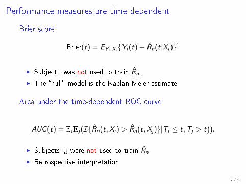
Performance measures are time-dependent

Brier score

Brier(t) = EYi ,Xi{Yi (t)− Rn(t|Xi )}2

I Subject i was not used to train Rn.

I The �null� model is the Kaplan-Meier estimate

Area under the time-dependent ROC curve

AUC (t) = EiEj(I{Rn(t,Xi ) > Rn(t,Xj)}|Ti ≤ t,Tj > t)).

I Subjects i,j were not used to train Rn.

I Retrospective interpretation

7 / 41

Uncensored observations

Time

Sta

tus

01

0 Ti

8 / 41

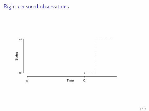
Right censored observations

Time

Sta

tus

01

0 Ci

9 / 41

Censored data problem

All performance parameters (expected Brier scores, concordanceprobabilities, etc.) depend on the unknown distribution of thefuture patients.

This data generating mechanism is best estimated by the empiricaldistribution of the validation data set.

However, when some patients are lost to follow-up (event-free)before the time horizon t, then their event status is unknown. Alsothe order of some pairs of patients is unknown (unusable).

In this case the performance parameters have to be estimated usingsome technique for right censored data to avoid bias.

10 / 41

Observations

Random variables

T event timeC censoring time

T = min(T ,C )∆ = 1{T ≤ C}X predictors

Assume (at least) that C is conditionally independent or T given X.

Otherwise the joint distribution of (T ,X ) is not identi�able fromthe observations.

11 / 41

Nuisance model

To deal with censoring, we need a second model (a nuisance) toestimate the distribution Ei of the validation data set. It is possible(but not recommended) to use the model whose performance isstudied.

However, when the aim is to compare two models, the nuisancemodel should de�nitely be independent of these two models.

Possible solutions:

I Inverse of probability of censoring weights (IPCW)

I Jackknife pseudo-values

Both depend on a model for the censoring distribution!

12 / 41

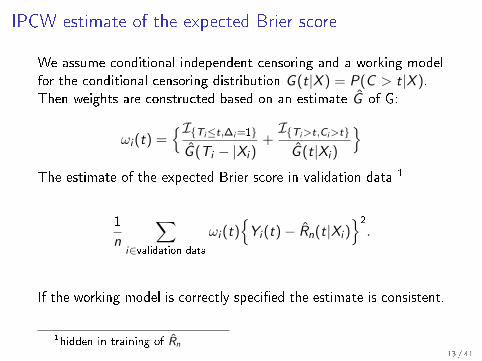
IPCW estimate of the expected Brier score

We assume conditional independent censoring and a working modelfor the conditional censoring distribution G (t|X ) = P(C > t|X ).Then weights are constructed based on an estimate G of G:

ωi (t) ={I{Ti≤t,∆i=1}

G (Ti − |Xi )+I{Ti>t,Ci>t}

G (t|Xi )

}The estimate of the expected Brier score in validation data 1

1

n

∑i∈validation data

ωi (t){Yi (t)− Rn(t|Xi )

}2

.

If the working model is correctly speci�ed the estimate is consistent.

1hidden in training of Rn13 / 41

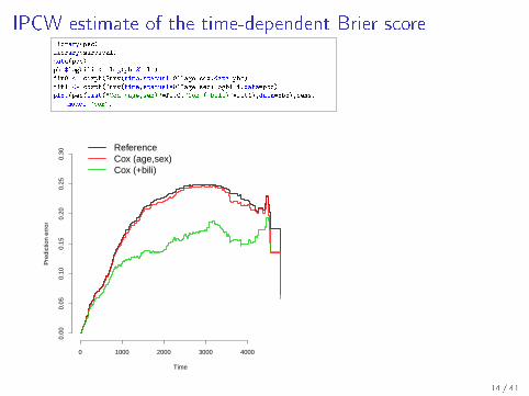
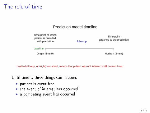
IPCW estimate of the time-dependent Brier scorelibrary(pec)

library(survival)

data(pbc)

pbc$logbili <- log(pbc$bili)

fit0 <- coxph(Surv(time,status!=0)~age+sex,data=pbc)

fit1 <- coxph(Surv(time,status!=0)~age+sex+logbili,data=pbc)

plot(pec(list("Cox (age,sex)"=fit0,"Cox (+bili)"=fit1),data=pbc),cens.

model="cox")

Time

Pre

dict

ion

erro

r

0 1000 2000 3000 4000

0.00

0.05

0.10

0.15

0.20

0.25

0.30

ReferenceCox (age,sex)Cox (+bili)

14 / 41

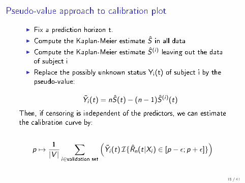
Pseudo-value approach to calibration plot

I Fix a prediction horizon t.

I Compute the Kaplan-Meier estimate S in all data

I Compute the Kaplan-Meier estimate S (i) leaving out the dataof subject i

I Replace the possibly unknown status Yi(t) of subject i by thepseudo-value:

Yi (t) = nS(t)− (n − 1)S (i)(t)

Then, if censoring is independent of the predictors, we can estimatethe calibration curve by:

p 7→ 1

|V |∑

i∈validation set

(Yi (t) I{Rn(t|Xi ) ∈ [p − ε; p + ε]}

)

15 / 41

Predicted event probability

0 % 25 % 50 % 75 % 100 %

Pse

udo−

obse

rved

eve

nt s

tatu

s

0 %

25 %

50 %

75 %

100 %

●

Calibration in the largebandwidth=1

Predicted event probability

0 % 25 % 50 % 75 % 100 %

Pse

udo−

obse

rved

eve

nt s

tatu

s

0 %

25 %

50 %

75 %

100 %

Localized calibrationbandwidth=0

Predicted event probability

0 % 25 % 50 % 75 % 100 %

Pse

udo−

obse

rved

eve

nt s

tatu

s

0 %

25 %

50 %

75 %

100 %

Kernel smootherautomatically selected

bandwidth= 0.194

Predicted event probability

0 % 25 % 50 % 75 % 100 %

Pse

udo−

obse

rved

eve

nt s

tatu

s

0 %

25 %

50 %

75 %

100 %

Kernel smootherbandwidth=0.1

16 / 41

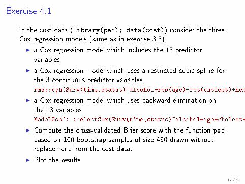
Exercise 4.1

In the cost data (library(pec); data(cost)) consider the threeCox regression models (same as in exercise 3.3)

I a Cox regression model which includes the 13 predictorvariables

I a Cox regression model which uses a restricted cubic spline forthe 3 continuous predictor variables.

rms::cph(Surv(time,status)~alcohol+rcs(age)+rcs(cholest)+hemor+...

I a Cox regression model which uses backward elimination onthe 13 variables

ModelGood:::selectCox(Surv(time,status)~alcohol+age+cholest+hemor+...

I Compute the cross-validated Brier score with the function pec

based on 100 bootstrap samples of size 450 drawn withoutreplacement from the cost data.

I Plot the results

17 / 41

Censored data & competing risks

It is sometimes not possible to observe very large or very smallvalues due to a detection limit.

In survival analysis the outcome is time-to-event and large valuesare not observed when the patient was lost-to-follow-up before theevent occurred.

Data are called right-censored when the event for a patient isunknown, but it is known that the event time exceeds a certainvalue.

A competing risk is an event after which it is clear that the patientwill never experience the event of interest.

18 / 41

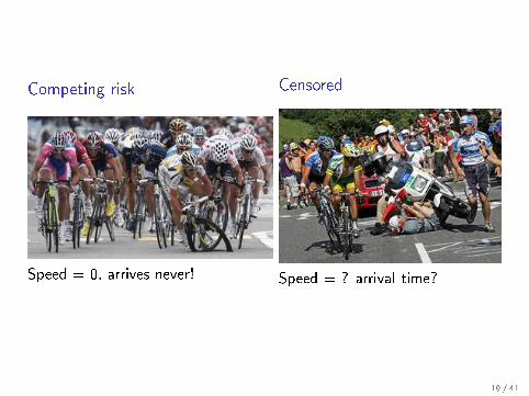
Competing risk

Speed = 0, arrives never!

Censored

Speed = ? arrival time?

19 / 41

Decision making in the presence of competing risks

Suppose a 40 year old and a 80 year old person need to decide foror against prophylactic coagulation therapy.

Suppose further the predicted risk of dying from cardiovasculardisease within the next 10 years for both persons is 12%. Howcould this happen?

One plausible explanation is that the 40 year old person has otherrisk factors that the 80 year old person does not have.

Another plausible explanation is that the 80 year old person has amuch higher risk to die due to non-cardiovascular disease within thenext 10 years than the 40 year old person.

20 / 41

Distinction between censored data and competing risks

What is the di�erence between censoring and (non-fatal)competing risks?

I Non-informative censoring does not change the event rates.

I A fatal competing risk changes the event rates from positiveto zero.

I Generally the occurrence of a competing risks changes theevent rate or changes the interest in the event (example:failure of a �lling in a primary tooth).

I In a competing risk model interest is in time to �rst event.What happens after the �rst event is not analysed.

I The e�ect of non-fatal events can also be studied in morecomplex multi-state models.

21 / 41

Competing risks

Any other event which changes the risk of the event being predictedmay be considered a separate state in a competing risk model.

Most commonly this would be dying from other causes.

Competing risks a�ect all stages of the process from the discoveryof markers over modelling and assessment of risk predictions tomedical decision making.

22 / 41

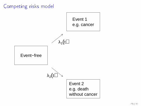
Competing risks model

Event−free

Event 1e.g. cancer

Event 2e.g. deathwithout cancer

λ1(t)

λ2(t)

23 / 41

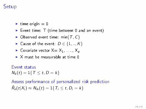
Setup

I time origin = 0

I Event time: T (time between 0 and an event)

I Observed event time: min(T ,C )

I Cause of the event: D ∈ {1, ..,K}I Covariate vector X= X1, . . . , Xp

I X must be measurable at time 0

Event statusNk(t) = 1{T ≤ t,D = k}

Assess performance of personalized risk prediction

Rn(t|Xi ) ≈ Nik(t) = 1{Ti ≤ t,Di = k}

24 / 41

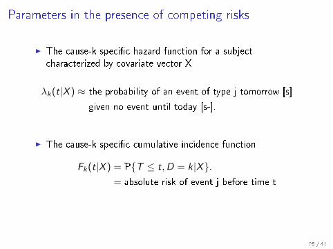
Parameters in the presence of competing risks

I The cause-k speci�c hazard function for a subjectcharacterized by covariate vector X

λk(t|X ) ≈ the probability of an event of type j tomorrow [s]

given no event until today [s-].

I The cause-k speci�c cumulative incidence function

Fk(t|X ) = P{T ≤ t,D = k |X}.= absolute risk of event j before time t

25 / 41

Prediction in the presence of competing risks

First pick a time origin at which it is of interest to predict thefuture status of a subject.

Until time t after the time origin three things can happen:

1. the event has occurred (e.g. cancer diagnosis)

2. a competing event has occurred (e.g. death without cancer)

3. the patient is alive and event-free.

When the individual observation period of a subject is shorter thantime t, the subject's event time is right censored.

26 / 41

Relation between hazards and absolute risks

Fk(t|X ) =∫ t

0

exp

(−∫ s

0

{λ1(u|X ) + · · ·+ λk(u|X )}du)

︸ ︷︷ ︸No event of any cause until s

λk(s|X )︸ ︷︷ ︸Event type j at s

ds.

I a covariate that reduces the cause-speci�c hazard of acompeting risk indirectly increases the cumulative incidence ofevent j .

I covariates found to change Fk are those that change any ofthe cause-speci�c hazard functions.

27 / 41

Di�erent tasks require di�erent methods

1. We focus on the cause-k speci�c hazard to identify variablesthat a�ect the biology of cause-k events:

I cause-speci�c log-rank test:

H0 : λk(t|A) = λk(t|B) = λk(t|C )I cause-speci�c Cox regressionI technique: treat competing events as if they were right

censored.

2. We focus on the cumulative incidence(s) to predict the risk(s)for patient counseling:

I Gray test:

H0 : Fk(t|A) = Fk(t|B) = Fk(t|C )I Combine cause-speci�c Cox regression modelsI Absolute risk regression modelI Fine-Gray regression model

28 / 41

Predicting event risk in presence of competing risks

The aim is to predict the absolute risk of an event of type 1, say,t-years after the time origin (or landmark):

F1(t|X) = cumulative incidence function

Common regression models for F1 are either based on:

F1(t|X ) =

∫ t

0

exp{− Λ1(s|X )− Λ2(s|X )

}Λ1(ds|X )

or

F1(t|X ) =

∫ t

0

P(min(T ,C ) > s|X )Λ1(ds|X )

G (s − |X )

29 / 41

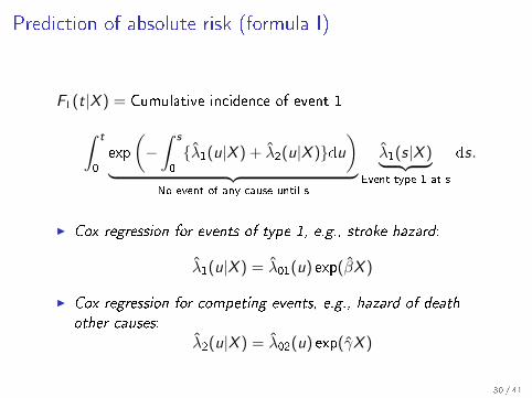
Prediction of absolute risk (formula I)

F1(t|X ) = Cumulative incidence of event 1∫ t

0

exp

(−∫ s

0

{λ1(u|X ) + λ2(u|X )}du)

︸ ︷︷ ︸No event of any cause until s

λ1(s|X )︸ ︷︷ ︸Event type 1 at s

ds.

I Cox regression for events of type 1, e.g., stroke hazard:

λ1(u|X ) = λ01(u) exp(βX )

I Cox regression for competing events, e.g., hazard of death

other causes:λ2(u|X ) = λ02(u) exp(γX )

30 / 41

Combination of cause-speci�c Cox regression

Remarks:

I A covariate that reduces the cause-speci�c hazard of acompeting risk indirectly increases the cumulative incidence ofevent j .

I covariates found to change the absolute risk of strokeI either change the cause-speci�c hazard of strokeI or change the cause-speci�c hazard of death other causesI or change both

Disadvantages:

I we need to model all competing risks or the overall survivalhazard function

I changes of the absolute risk depend on changes of a singlecovariate in a complicated way

31 / 41

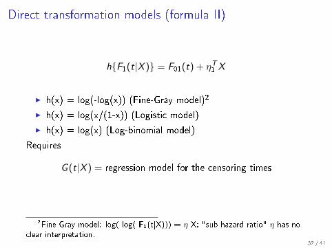
Direct transformation models (formula II)

h{F1(t|X )} = F01(t) + ηT1 X

I h(x) = log(-log(x)) (Fine-Gray model)2

I h(x) = log(x/(1-x)) (Logistic model)

I h(x) = log(x) (Log-binomial model)

Requires

G (t|X ) = regression model for the censoring times

2Fine-Gray model: log(-log(-F1(t|X))) = η X; "sub-hazard ratio" η has noclear interpretation.

32 / 41

Prediction of absolute risk (formula II)

It would be desirable to have a model in which the regressioncoe�cients β have the following interpretation:

The absolute risk of a stroke during the next 't' years changes with

a factor exp(β) for a one unit change of age, given �xed values for

the other predictor variables.

Absolute risk regression:3

F1(t|X ) = F01(t) exp(βX ) (Log-binomial model)

Disadvantages:

I estimation of β requires a (regression) model for theprobability of not being lost to followup, i.e., a regressionmodel for the censoring times.

I model has numerical problems with e�ects of continuouscovariates

3Absolute risk regression (Stat. med., 2012, 31, 3921�30)33 / 41

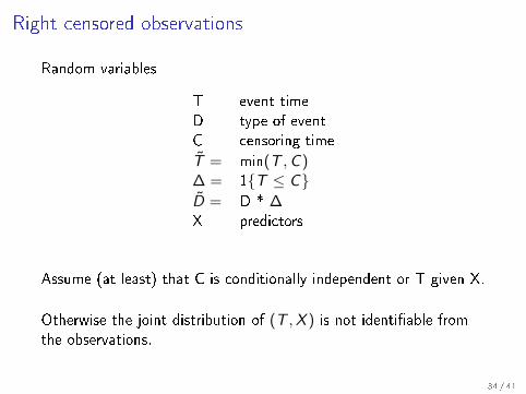
Right censored observations

Random variables

T event timeD type of eventC censoring time

T = min(T ,C )∆ = 1{T ≤ C}D = D * ∆X predictors

Assume (at least) that C is conditionally independent or T given X.

Otherwise the joint distribution of (T ,X ) is not identi�able fromthe observations.

34 / 41

Brier score in the presence of competing risks

Brier(t, k) = ET ,D,X{Nk(t)− Rn(t|Xi )}2

I Null model is Aalen-Johansen estimate

IPCW estimate of the expected Brier score (cause k)

We need a "working model" and a corresponding estimate G forthe conditional censoring distribution G (t|X ) = P(C > t|X )

1

n

∑i∈validation data

{I{Ti≤t,∆i=1}

G (Ti − |Xi )+I{Ti>t,Ci>t}

G (t|Xi )

}{Nik(t)−Rn(t|Xi )

}2

.

If the working model is correctly speci�ed the estimate is consistent.

35 / 41

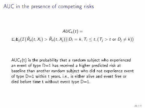
AUC in the presence of competing risks

AUCk(t) =

EiEj(I{Rn(t,Xi ) > Rn(t,Xj)}|Di = k,Ti ≤ t, (Tj > t or Dj 6= k))

AUC1(t) is the probability that a random subject who experiencedan event of type D=1 has received a higher predicted risk atbaseline than another random subject who did not experience eventof type D=1 within t years, i.e., is either alive and event free ordied before time t without event type D=1.

36 / 41

IPCW estimate of AUC (cause k)

Weights:

Wij ,1 =I{Ti<Tj ,Ti<Ci}

G (Ti − |Xi )G (Ti |Xj)

Wij ,2 =I{Ti≥Tj ,Dj 6=k,Tj≤Cj}

G (Ti − |Xi )G (Tj − |Xj)

IPCW estimate:∑i ,j∈validation data

(Wij ,1 + Wij ,2

)I{Rn(t,Xi )>Rn(t,Xj )}Nik(t)∑

i ,j∈validation data

(Wij ,1 + Wij ,2

)Nik(t)

Note: I{Rn(t,Xi )>Rn(t,Xj )} may change over time.

37 / 41

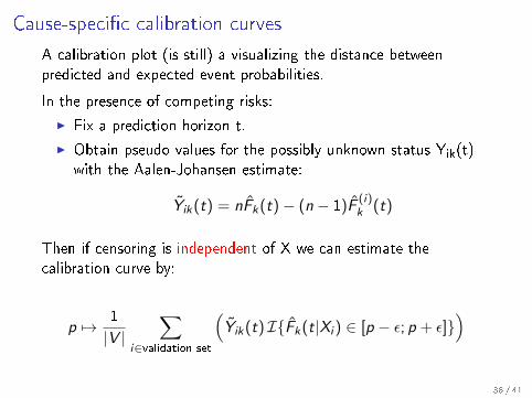
Cause-speci�c calibration curves

A calibration plot (is still) a visualizing the distance betweenpredicted and expected event probabilities.

In the presence of competing risks:

I Fix a prediction horizon t.

I Obtain pseudo values for the possibly unknown status Yik(t)with the Aalen-Johansen estimate:

Yik(t) = nFk(t)− (n − 1)F(i)k (t)

Then if censoring is independent of X we can estimate thecalibration curve by:

p 7→ 1

|V |∑

i∈validation set

(Yik(t) I{Fk(t|Xi ) ∈ [p − ε; p + ε]}

)

38 / 41

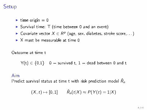
Example

●

●

●

●●

●

●

●

●

●

●

●●

●

●●

●

●

●

●

●●

●●

●

●

●●

●

●

●●

●

●

●●

●

●

●

●

●

●

●

●

●

●●

●●

●

●

●

●●●●

●

●●

●●●

●

●

●

●

●

●

●

●●

●

●

●

●

●

●

●

●

●●

●

●●●

●

●

●

●

●

●●

●

●

●

●

●

●

●

●

●●

●

●●●

●

●

●

●

●

●

●

●

●

●

●

●

●

●

●

●

●

●●

●

●

●

●

●

●

●●

●

●

●

●

●

●

●

●

●

●

●

●

●

●●

●

●

●

●

●

●

●

●●●

●●

●

●

●

●

●●●

●

●

●

●

●

●

● ●

●

●

●

●

●

●

●

●

●●

●●

●

●

●

●

●

●

●

●

●

●

●

●

●

●

●

●

●●

●

●●●

●

●●

●

●

●●

●

Multiple regressionwithout ERG status

2−yr prediction horizon

Risk reclassification

●

●

ERG status

NegativePositive

Multiple regressionwith ERG status

0 % 25 % 50 % 75 % 100 %

0 %

25 %

50 %

75 %

100 %

Multiple regression with ERG status

0 % 25 % 50 % 75 % 100 %

0 %

25 %

50 %

75 %

100 %

2−yr prediction horizon

Calibration

Observedprobabilities

Years on AS

0 1 2 3 4

0 %

10 %

20 %

30 %Reference (no predictor variables)Multiple regression without ERG statusMultiple regression with ERG status

Prediction error

Years on AS

0 1 2 3 4

40 %

50 %

75 %

100 % Reference (no predictor variables)Multiple regression without ERG statusMultiple regression with ERG status

Discrimination ability

39 / 41

Summary and conclusions

In survival analysis predictions and prediction performance aretime-dependent. Performance is a parameter (of the distribution ofthe validation data) which needs to be estimated usually in thepresence of right censored data.

With competing risks the way we do things need some slightadaptation, there are pitfalls, and some formula get more complex,but generally everything seems to be under control.

To interprete a prediction in most applications with competing riskswe have to build several models, one for each competing risk.

40 / 41

Exercise 4.2

I Work through the appendix of Absolute risk regression (seecourse homepage).

I In the pbc data library(survival); data(pbc)

I compute a cause-speci�c Cox regression model with thefunction CSC

I compute a Fine-Gray regression model for cause 2 with thefunction FGR

I predict the event risk of cause 2 with both methods, assessand compare their prediction performance. Hint: uselibrary(pec) for Brier score and library(timeROC) forROC and AUC.

41 / 41