Surveyor Handbook for River Campus 2014

River Campus Restoration Monitoring: Surveyor Handbook

University of Portland

Assembled by Katelin D. Stanley following the summer 2014 field season

1

Contents Introduction .............................................................................................................................................. 3

River Campus Riparian Zone Survey Area ................................................................................................. 3

Woody Plant Inventory ............................................................................................................................. 5

Objectives .............................................................................................................................................. 5

Timeline ................................................................................................................................................. 5

Materials ............................................................................................................................................... 5

Procedure .............................................................................................................................................. 5

Special Notes ......................................................................................................................................... 9

Identification ....................................................................................................................................... 10

Analysis and Presentation ................................................................................................................... 11

Suggested Comparative Analysis ........................................................................................................ 11

Avian Surveys .......................................................................................................................................... 12

Objectives ............................................................................................................................................ 12

Timeline ............................................................................................................................................... 12

Materials ............................................................................................................................................. 12

Procedure ............................................................................................................................................ 12

Data Collection .................................................................................................................................... 13

Special Notes ....................................................................................................................................... 14

Identification ....................................................................................................................................... 14



Invertebrate Surveys ............................................................................................................................... 16

Objectives ............................................................................................................................................ 16

Timeline ............................................................................................................................................... 16

Materials ............................................................................................................................................. 16

Procedure ............................................................................................................................................ 16

Data Collection .................................................................................................................................... 19

Special Notes ....................................................................................................................................... 20

Identification ....................................................................................................................................... 21



2

Vegetation Surveys ................................................................................................................................. 22

Timeline ............................................................................................................................................... 22

Materials ............................................................................................................................................. 22

Procedure ............................................................................................................................................ 22

Data Collection .................................................................................................................................... 24

Special Notes ....................................................................................................................................... 25

Identification ....................................................................................................................................... 25



Index of Figures and Tables .................................................................................................................... 28

3

Introduction The purpose of this research is to provide ecological data in terms of plant, avian, and insect

diversity over the course of several summer field seasons. In addition, data will be analyzed spatially and

temporally in order to monitor the health of the riparian zone and support recommendations for future

restoration and study, with the ultimate goal of improving this area to support native species such as

salmon. See the 2014 report of Stanley and Bauer for full introduction.

River Campus Riparian Zone Survey Area In May 2014, the riparian zone of the University of Portland River Campus was divided into 16

sections delineated by 16 transects (Figure 1). Transects were marked by placing flags at 50 meter

increments along the road edge (GPS coordinates in Table 1). An additional flag was placed at the

shoreline in line with the first flag so as to make a perpendicular line from the road to the Willamette

River. Notably, many of the flags at the shoreline were washed away by the end of the 2014 season.

Transects were numbered sequentially from 1-16, with transect 1 at the southernmost end.

Areas between transects were named, from South to North, as follows: Alpha, Bravo, Charlie,

Delta, Echo, Foxtrot, Golf, Hotel, India, Juliet, Kilo, Mike, November, Oscar (Figure 1). Sector Alpha was

the area between transects 1 and 2, Bravo between 2 and 3, et cetera. The sector between the

southernmost edge of the property and the first transect was labeled as sector Null (0), as it was

significantly smaller and rockier than the other fifteen sections and was not to be included in analysis

other than woody plant inventory.

Table 1: GPS coordinates of vegetation survey transects and avian point count locations Transect Latitude Longitude

1 45°34'18.896 N 122°43'57.822 W

2 45°34'19.975 N 122°43'59.606 W

3 45°34'21.034 N 122°44'01.337 W

4 45°34'21.867 N 122°44'03.319 W

5 45°34'23.238 N 122°44'04.144 W

6 45°34'24.803 N 122°44'03.655 W

7 45°34'25.763 N 122°44'05.491 W

8 45°34'26.678 N 122°44'07.287 W

9 45°34'27.904 N 122°44'08.754 W

10 45°34'28.714 N 122°44'10.763 W

11 45°34'29.754 N 122°44'12.000 W

12 45°34'29.641 N 122°44'14.168 W

13 45°34'29.306 N 122°44'16.260 W

14 45°34'30.283 N 122°44'18.110 W

15 45°34'31.751 N 122°44'17.942 W

16 45°34'32.551 N 122°44'16.870 W

Avian Point Count Locations

HAWK 45°34'31.935 N 122°44'17.889 W

IRON 45°34'27.287 N 122°44'07.783 W

THOR 45°34'20.735 N 122°44'01.036 W

4

Figure 1: Representation of River Campus riparian area division into designated transects and sectors. Yellow

circles correspond to avian point count locations: top = HAWK, center = IRON, bottom = THOR.

North

5

Woody Plant Inventory

Objectives

Produce a map of locations and conditions of all trees in the River Campus riparian zone

Tally the number, species, and conditions of woody plants in the River Campus riparian zone

Timeline

Inventory should be completed in late May, as close to the dates listed in Table 2 as possible

An additional shoreline walkthrough may be necessary in late July-August, depending on water

levels (see Special Notes: Willows)

Table 2: Dates of woody plant inventory for each field season. Please update this table every season.

Field Season Date Range

2014 May 21 - 27

2015

2016

2017

Materials

Data sheets

Pencil/pens

Field measuring tape

Woody plant inventory map

Condition descriptions table (Table 3)

Woody plant identification booklet, for reference

Procedure

1. Begin inventory with sector Null (0) and progress northward (Alpha Oscar).

2. Fill out the sector and date of survey on the data sheet.

3. Measure and record all four dimensions of the sector.

4. Both surveyors should walk side by side, beginning near the shoreline to observe every woody

plant. One surveyor should be responsible for all woody plants observed between him/her and

the shoreline (looking to the left, for example), while the other is responsible for all woody

plants observed between him/her and a given distance away (3-4 meters).

a. See the PowerPoint animation “How to Survey Woody Plants” for clarification

(summarized in Figure 2).

5. Tally the species and condition of each woody plant observed (see Table 3 for reference).

6. The locations of trees (see species under the heading “Trees” in Table 5) should be verified on

the woody plant inventory map. If the individual is still found in the same location and in the

same condition, give it a checkmark. If the individual is not found or is dead, cross it out with an

6

‘X’. If the individual has changed conditions, indicate this on the map with an appropriate letter

or color.

7. To ensure all woody plants are accounted for, it is suggested to cross the length of the sector a

minimum of three times (see Figure 2).

Figure 2: How to conduct woody plant inventory. The route which both surveyors follow is shown by the dotted

red arrows. The starting points for the surveyors are shown on the bottom right, along with their lines of sight

during the inventory (Surveyor 1 in blue and Surveyor 2 in orange). This pattern should be repeated every sector.

This figure can be better understood by viewing the “How to Survey Woody Plants” PowerPoint animation.

7

Table 3: Woody plant condition classifications and representative photographs

Condition Qualifications Example Photos

Poor - Visibly damaged/stressed

- Red, yellow, or otherwise discolored

foliage

- Heavy flowering/fruiting with minimal

vegetative growth

- Dead branches

Fair - Minor signs of damage or stress

- Some discoloration acceptable, but vegetative growth generally well formed and lacking damage

Good - Obviously healthy foliage, no

discoloration or damage - No signs of stress

8

Data Collection

A separate data sheet should be filled out for each sector (total of 16 data sheets) (Table 4)

Make sure to fill out the first section (date, dimensions, etc.) before beginning the survey

Table 4: Data sheet for woody plant inventory

Sector Date Shoreline width Roadside width N length S length

Poor Fair Good SHRUBS

Bald-hip rose Indian plum Nootka rose Oceanspray Pacific ninebark Red currant Red elderberry Red-osier dogwood Serviceberry Snowberry Twinberry Yellow currant WILLOWS Salix spp. TREES

Aspen Black cottonwood Cascara sagrada Columbian hawthorn Douglas fir Oregon ash Red alder Vine maple

9

A small segment of the woody plant inventory map is shown in Figure 3. Each tree (see species

under the heading “Trees” in Table 5) should be verified on the map. If the individual is still

found in the same location and in the same condition, give it a checkmark. If the individual is not

found or is dead, cross it out with an ‘X’. If the individual has changed conditions, indicate this

on the map with an appropriate letter or color.

Figure 3: Mapped locations and conditions of woody plants for sectors Alpha-Delta. (Green = good, yellow = fair,

orange = poor) (A = Oregon ash, AL = Red alder, AS = Quaking aspen, C = Cottonwood, CS = Cascara, DF = Douglas

fir, H = Columbian hawthorn, V = Vine maple)

Special Notes

Ash/Cottonwood Saplings

Oregon ash and black cottonwood are prolific natives of the area and thus may be observed

outside the regular planting lines. Regardless, they are to be included in the woody plant

inventory.

Large clusters of Oregon ash saplings can often be found along the shore or floating just

offshore, clinging to the sand by a couple strands of root. These are to be counted (or estimated,

if a very large quantity) and included in the tally.

Dead Plants

Completely dead individuals (only a stick visible, no leaves at all) should not be included in the

inventory.

Following the Pattern

Woody plants were planted in semi-regular intervals along rows, which can be useful in

predicting where you will next find an individual, especially when that individual may be hidden

beneath tall grasses or lupine. Hanna and Katie observed that there were four distinct rows of

plantings (disregarding the willow stakes).

Plants that Hide

Pay close attention to where woody plants might be. Because of their stunted growth, many get

lost under tall grasses or lupine and might therefore be overlooked (see note above).

10

Volunteer woody plants

Some woody plants not planted by UP have become established in the riparian zone as well.

These plants, except for Oregon ash and black cottonwood, should not be included in the

survey. Volunteers can be identified by location (not within the normal planting line), species

(not found in Table 5), and a lack of bark chips at the base.

Willows

Due to changing water levels, willows along the shoreline and submerged in the river should be

counted as best as possible given the water level at the time of inventory. You may need to

conduct a second inventory later in the season (late July to early August) in which you walk

along the bottom edge of the riparian zone and count the number of willow stakes which

present leaves.

Willows are generally only identified as Salix spp.

Identification

See Woody Plant Identification Booklet

Woody plants identified on River Campus during the summer 2014 season are shown in Table 5

Table 5: List of woody plant species identified on River Campus during the summer 2014 season

SHRUBS

Serviceberry Amelanchier alnifolia

Red-osier dogwood Cornus sericea

Ocean Spray Holodiscus discolor

Twinberry Lonicera involucrata

Indian plum Oemlaria cerasiformus

Pacific ninebark Physocarpus capitatus

Yellow flowering currant Ribes aureum

Red flowering currant Ribes sanguineum

Nootka rose Rosa nutkana

Red elderberry Sambucus racemosa

Snowberry Symphoricarpos albus

WILLOWS

Pacific willow Salix lasiandra

Scouler’s willow Salix scouleriana

Sitka willow Salix sitchensis

TREES

Vine maple Acer circinatum

Red alder Alnus rubra

Columbian hawthorn Crataegus columbiana

Oregon ash Fraxinus latifolia

Black cottonwood Populus trichocarpa

Douglas fir Pseudotsuga menziesii

Aspen Populus tremuloides

Cascara sagrada Rhamnus purshiana

Willows were only identified as

Salix spp. during the 2014 season

due to minimal growth. This list

represents species which were

reportedly planted.

11

Analysis and Presentation

Spreadsheet

The main analysis spreadsheet is titled “Woody Plant Inventory Data.”

Enter the data exactly as it appears on your data sheets. Each sector has its own tab/sheet in the

spreadsheet.

Once each tab has been populated, the data can be found summarized in the “Summary”

tab/sheet. This tab/sheet shows the total and percent survival of the inventoried woody plant

species and compares it to the reported total that was planted by UP.

The “Conditions Summary” tab/sheet will also be populated automatically once each sector

tab/sheet has been filled out. This will produce a pie chart that expresses the percentage of

plants in each health condition (poor, fair, or good).

Woody Plant Inventory Map

Using a copy of the original woody plant inventory map images, a new woody plant inventory

map should be constructed to show the most recent season’s survey.

Suggested Comparative Analysis

Compare planted totals to observed totals of woody plants across field seasons

Compare trends in woody plant condition across field seasons

Compare the inventory maps across field seasons to observed trends in woody plant mortality A

suggested method is to juxtapose the 2014 tree inventory data with a new list containing the

changes (indicated by X’s and condition changes on the map). Then pull any interesting statistics

from there such as:

a. Number of trees which improved in condition since last field season

b. Number of trees which have died since last field season

c. Any change in community composition (is any one species clearly doing better than the

others?)

12

Avian Surveys

Objectives

Provide a weekly snapshot of avian life utilizing the River Campus riparian zone using the avian

point count method

Timeline

Surveys should be conducted weekly at each of the three point count stations beginning in the

third week in May and ending in the third week of July (Table 6)

One set of weekly surveys should be conducted between 0800 and 1000 hours (8:00-10:00AM)

A second collection of weekly surveys may be conducted in which the time of the survey is

determined by random number generation.

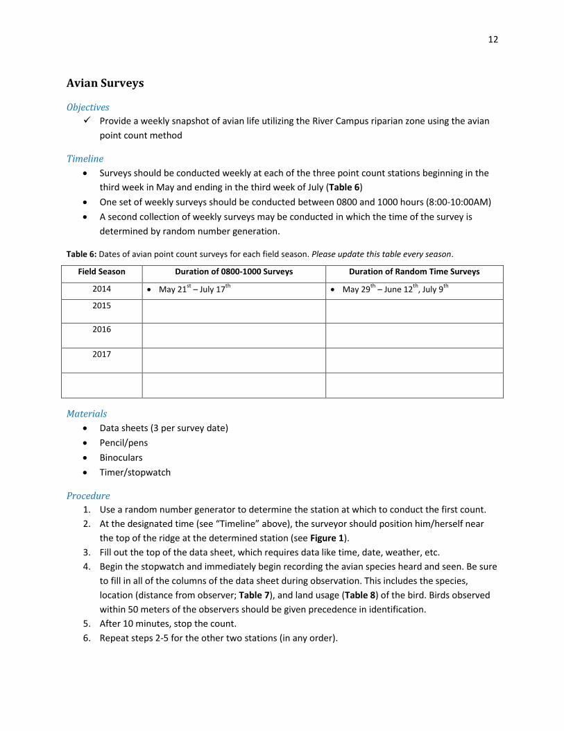
Table 6: Dates of avian point count surveys for each field season. Please update this table every season.

Field Season Duration of 0800-1000 Surveys Duration of Random Time Surveys

2014 May 21st

– July 17th

May 29th

– June 12th

, July 9th

2015

2016

2017

Materials

Data sheets (3 per survey date)

Pencil/pens

Binoculars

Timer/stopwatch

Procedure

1. Use a random number generator to determine the station at which to conduct the first count.

2. At the designated time (see “Timeline” above), the surveyor should position him/herself near

the top of the ridge at the determined station (see Figure 1).

3. Fill out the top of the data sheet, which requires data like time, date, weather, etc.

4. Begin the stopwatch and immediately begin recording the avian species heard and seen. Be sure

to fill in all of the columns of the data sheet during observation. This includes the species,

location (distance from observer; Table 7), and land usage (Table 8) of the bird. Birds observed

within 50 meters of the observers should be given precedence in identification.

5. After 10 minutes, stop the count.

6. Repeat steps 2-5 for the other two stations (in any order).

13

Table 7: Codes to use when indicating the location of observed birds in the “Location” column of the point count

data sheet.

Location Designation

Conditions

1 -Within 50 meters of observer OR -Within the riparian zone (area under restoration)

2 -50-100 meters away from observer

3 -Over 150 meters away from observer

Table 8: Codes to use when indicating the land usage of observed birds in the “Land Use” column of the point

count data sheet.

A air (flying)

G ground

P pier (manmade structures just offshore)

U unknown (bird heard, not seen)

V vegetation (on tree or shrub)

W water (swimming/floating)

Data Collection

A separate data sheet should be filled out for each point count location (total of 3 data sheets

per survey) (Table 9)

Make sure to fill out the first section (point, date, etc.) before beginning the survey

Table 9: Truncated data sheet for avian point count survey

Point Date Time Weather Wind

Species Location (1,2,3) Land Use (W,A,G,V,U,P)

1

2

3

4

5

6

7

8

etc.

0 Clear or few clouds

1 Partly cloudy

2 Mostly cloudy/overcast

3 Foggy

4 Drizzle

5 Rain

0 No wind

1 Slight breeze, not much leaf movement

2 Leaf movement

3 Leaf and small branch movement

4 Branch movement

5 Small tree/branch movement

6 Large tree/branch movement

Weather

Wind

14

Special Notes

Binoculars

Binoculars are helpful to use once the surveyor has written all of the individual birds down and

would like to identify the specific species of, for example, swallow.

Swallows

Swallows are difficult to identify due to their speed and abundance. It may be helpful to count

the individuals at the beginning of the count as UNSW and then identify them during or after the

count.

Using calls and songs of swallows may be useful for identification purposes, as each of the

different species has a characteristic call during flight.

Weather

Point counts should not be conducted during rainy, stormy, or excessively windy conditions.

Identification

Avian species identified on River Campus during the summer 2014 season are shown in Table 10

Avian species can be identified using their songs, calls, and visual characteristics. Good resources

to use for identification include:

Online Resources

o Cornell Lab of Ornithology Bird Guide: <www.allaboutbirds.org>

o Oregon Department of Fish and Wildlife, Oregon Wildlife Species:

<http://www.dfw.state.or.us/wildlife/diversity/species/index.asp >

Book Resources

o Burrows, R. and J. Gilligan. 2003. Birds of Oregon. Auburn, WA: Lone Pine Publishing.

o Sibley, D. A. 2003. The Sibley Field Guide to Birds of Western North America. New York

City, NY: Knopf Doubleday Publishing Group.

Table 10: List of avian species identified on River Campus during the summer 2014 season

Family Species Family Species

Accipitridae Red tailed hawk Emberizidae Oregon junco Alcedinidae Belted kingfisher Fringillidae American goldfinch Anatidae Canada goose House finch Mallard Hirundinidae Violet-green swallow Anatidae Common merganser Barn swallow Apodidae Vaux’s swift Cliff swallow Ardeidae Great blue heron Tree swallow

Bombycillidae Cedar waxwing Icteridae Brown headed cowbird Cardinalidae Lazuli bunting Laridae Gull spp. Cathartidae Turkey vulture Pandionidae Osprey

Charadriiae Killdeer Scolopacidae Spotted sandpiper Columbidae Mourning dove Sturnidae European starling Rock dove Trochilidae Hummingbird spp. Corvidae American crow Turdidae American robin Emberizidae White-crowned sparrow

15


Even if data concerning avian species outside the River Campus riparian zone was collected,

statistical analysis should only be performed using data from birds observed in location “1.”

Spreadsheet

The main analysis spreadsheet is titled “Avian Survey Data.”

Enter the data into each of the sheets labeled according to their survey point (HAWK, IRON, or

THOR). The number of individuals of each bird species should be placed in the “Tally” column

and the land usage of the individuals should be placed in the “Land Use” column.

If there are multiple different land uses for a species, input them in the same row separated by

commas.

Once the spreadsheet has been populated, the diversity indices, species richness, and species

evenness of each survey will be automatically calculated and can be found at the bottom of the

sheet.

In the bottom left, surrounded by a thick black border, is a summary table that lists the following

for all survey dates combined:

o Average diversity index (+ standard deviation and standard error of the mean)

o Average species richness (+ standard deviation and standard error of the mean)

o Average number of birds total (+ standard deviation and standard error of the mean)

o Average evenness (+ standard deviation and standard error of the mean)

If second weekly surveys at random times are conducted, their data should be entered into a

separate spreadsheet (a copy of the “Avian Survey Data” spreadsheet).

Tables to Include in Final Report:

List of avian species observed using the riparian zone

Average diversity index, species richness, number of birds total, and evenness + standard

deviation and standard error of the mean for the 0800-1000 surveys and random time surveys

(separately, if applicable)

Any comparative analysis


Compare the progression of avian activity between field seasons

Compare avian diversity, species richness, number of birds and evenness between survey points

and field seasons

Compare community composition between field seasons

16

Invertebrate Surveys

Objectives

Provide a snapshot of invertebrate diversity during the field season by capturing invertebrates

using three different methods in sequence

Timeline

Collections should be completed as close to the dates listed in Table 11 as possible

Table 11: Dates of invertebrate collection for each field season. Please update this table every season.

Field Season Date Range

2014 7 collections between June 6th and 11th

7 collections between July 7th and 17th

2015

2016

2017

Materials

Data sheets (1 per capture session)

Pencil/pens

Small plastic vials (100-150)

Plastic/paper bags and/or boxes to hold collections of vials

Sharpie

Tape (for labeling collections)

Two 38-cm sweep nets

Disposable gloves

Quadrat


Timer/watch

Procedure

One collection session is comprised of three methods employed consecutively:

ground/vegetation searching, targeted netting, and aerial sweeping.

A total of 14 collection sessions should be performed according to the timeline outlined above

Invertebrates should be stored for at least an hour in the freezer prior to sorting and counting

17

INSECT COLLECTION

Ground/vegetation searching

1. Use a random number generator to come up with:

a. Number “p” such that 1 ≤ p ≤ 16

i. This number should not be used more than once for invertebrate collection

sessions in one season. In other words, don’t visit a transect more than once to

collect invertebrates.

b. Number “q” such that 1 ≤ q ≤ maximum number of quadrats in transect “p”

2. Set the quadrat at transect “p” and quadrat number “q”

a. Start from the shoreline at odd-numbered transects and at the road for even-numbered

transects. For example, if p = 3 and q = 2, set up transect 3 and then place the quadrat at

5.5 m from the shoreline (0.5 m = quadrat 1, 5.5 m = quadrat 2).

3. Fill out the first three rows of the invertebrate datasheet.

4. Before starting the timer, make sure that each collector is wearing gloves (if preferred) and has

a nearby collection of plastic vials with which to capture invertebrates.

5. For exactly 10 minutes, both collectors (there must be two) should capture every possible insect

observed within the quadrat area into individual plastic vials. This may necessitate scooping the

insect with the vial, grabbing the insect with a (gloved) hand and placing it into the vial, trapping

the insect in the vial, or other creative methods to ensure collection.

a. If a semi-stationary colony is observed (of ants or aphids, for example), the number of

individuals may be counted instead of all captured.

b. If an insect proves difficult to capture due to speed, etc. note what type of insect it is in

the data notebook and approximately how many were observed but not captured.

6. Properly label the collection of vials (date, location, method of capture) and keep them separate

from collections obtained via other sampling methods by storing in paper/plastic bags or

containers.

Targeted Netting

1. Set up two transect measuring tapes, one at each border of the sector North of transect “p”

(determined above, see Table 12).

Table 12: Target/aerial collection sectors corresponding to given transect numbers as randomly determined for

ground/vegetation collection method

Transect number (p) Sector for collection Transect number (p) Sector for collection

1 Alpha 9 India

2 Bravo 10 Juliet 3 Charlie 11 Kilo

4 Delta 12 Lima 5 Echo 13 Mike

6 Foxtrot 14 November 7 Golf 15 Oscar

8 Hotel 16 Use sector that will not be surveyed

18

2. Before starting the timer, make sure that each collector (2) has gloves, a 38 cm sweep net, and a

sufficient collection of plastic vials on their person.

3. For exactly 10 minutes, both collectors should actively capture all conspicuous flying insects in

the allotted sector by chasing and sweeping them into the net. “Conspicuous flying insects”

generally include larger insects such as flies, wasps, grasshoppers, ladybugs, flying beetles, bees,

moths, butterflies, etc. Note that some of these (grasshoppers, beetles) may fly for a short time

before landing in the sector, but they may be included in collection.

a. The best way to capture a flying insect is to sweep sideways where it is flying, then

constrict the net with your hand to trap the insect in the end of the net.

b. If the pursuit of a single individual insect occupies 45-60 seconds of the allotted time,

stop chasing it and simply record its presence.

4. Seal each insect in an individual vial.

a. You may try inserting a vial into the end of the net (where the insect is trapped),

cornering the insect with the vial by manipulating it from outside the net, and then

closing the vial with both hands still outside the net.



containers.

6. Record the presence and relative abundance of other insects observed but not captured during

the 10 minute collection time. This is especially important for bees, as you will not be able to

capture them all (see “Bees” in Special Notes).

Aerial Sweeping

1. Use the same sector as was delineated for targeted netting.

2. For 5 minutes, both collectors should continuously sweep the air with nets in a side-to-side

figure-8 motion while walking a random path within the sector.

3. Immediately after the allotted time is done, constrict the net with one hand as close to the

mouth of the net as possible to trap all insects inside.

4. Collect all of the insects in the net into plastic vials. Methods with previous success include:

a. Have one collector hold the mouth of the net loosely constricted in one hand while

slowly pulling it inside out with the other hand. While the first collector does this, the

second collector traps all the insects which emerge from the opening at the first

collector’s hand.

b. In case of a very large collection of gnats, you may wish to collect the larger insects first

via method “a,” then collect all of the remaining insects by quickly inverting the net

inside a plastic bag, shaking to loosen the insects, and then tying off the bag.

c. If there are many bees active in the sector, it is acceptable to count the captured bees

(carefully recording this number) and then release them once all collection sessions are

done.

5. Double-check the net for any missed insects.



containers.

19

INSECT PRESERVATION

1. Place all collected insects (carefully labeled and distinguishable from all other collection dates

and methods) in a freezer for at least an hour before sorting.

INSECT SORTING AND COUNTING

1. Once the insects are frozen, dump all the individual vials from one collection date and method

into a plastic petri dish.

2. Carefully label a pillbox with the date, location, and method of collection of the sample.

3. Label each chamber of the pillbox with the name of an invertebrate order found in your sample

(you will need to glance at your sample first to do this).

4. Sort the insects according to taxonomic order (see “Identification”) into the appropriately

labeled pillbox, placing the orders in separate chambers.

5. Once all the insects in the sample are sorted, count the number of individuals in each order

using a counter and record this data in the invertebrate collection spreadsheet.

Data Collection

A separate data sheet should be filled out for each collection session (total of 14 data sheets)

(Table 13)

o Before beginning collection, rows 1-3 of the datasheet should be filled out.

o After this, only the bottom row (21) will be used during the collection session to record

invertebrates that are observed but not captured.

o Rows 5-20 are filled out when counting the number of invertebrates after freezing and

sorting.

See Table 12 for determining which sector in which to capture insects during aerial/targeted

netting

20

Table 13: Datasheet for capture and counting of invertebrates

1 Sector/Transect/Quadrat

2 Date/Time

3 Weather conditions

4 Aerial Ground Target

5 Acari

6 Araneae

7 Chilopoda

8 Coleoptera

9 Collembola

10 Diptera

11 Hemiptera

12 Homoptera

13 Hymenoptera

14 Lepidoptera

15 Neuroptera

16 Odonata

17 Opilones

18 Orthoptera

19 Thysanoptera

20 Unknown

21 Observed but not captured

Special Notes

Bees

During the later months, honeybees and bumblebees become so abundant that capturing them

during targeted netting would consume all of the allotted 10 minutes. When this is the case,

note their abundance under “insects observed but not captured during targeted collection” and

focus on capturing other species

Bonus Captures

During targeted netting, it is acceptable to collect an insect from inside your net even if it was

not the one you were targeting. However, this should be done only sparingly and most of the

time should be spent hunting for insects, not collecting “bonus captures” in vials.

Time of Day

Though no randomization procedure was developed due to collector availability, the time of

insect capture should vary between the hours of 0900 and 1600.

21

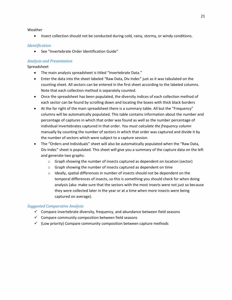
Weather

Insect collection should not be conducted during cold, rainy, stormy, or windy conditions.

Identification

See “Invertebrate Order Identification Guide”


Spreadsheet

The main analysis spreadsheet is titled “Invertebrate Data.”

Enter the data into the sheet labeled “Raw Data, Div Indec” just as it was tabulated on the

counting sheet. All sectors can be entered in the first sheet according to the labeled columns.

Note that each collection method is separately counted.

Once the spreadsheet has been populated, the diversity indices of each collection method of

each sector can be found by scrolling down and locating the boxes with thick black borders

At the far right of the main spreadsheet there is a summary table. All but the “Frequency”

columns will be automatically populated. This table contains information about the number and

percentage of captures in which that order was found as well as the number percentage of

individual invertebrates captured in that order. You must calculate the frequency column

manually by counting the number of sectors in which that order was captured and divide it by

the number of sectors which were subject to a capture session.

The “Orders and Individuals” sheet will also be automatically populated when the “Raw Data,

Div Indec” sheet is populated. This sheet will give you a summary of the capture data on the left

and generate two graphs:

o Graph showing the number of insects captured as dependent on location (sector)

o Graph showing the number of insects captured as dependent on time

o Ideally, spatial differences in number of insects should not be dependent on the

temporal differences of insects, so this is something you should check for when doing

analysis (aka: make sure that the sectors with the most insects were not just so because

they were collected later in the year or at a time when more insects were being

captured on average).


Compare invertebrate diversity, frequency, and abundance between field seasons


(Low priority) Compare community composition between capture methods

22

Vegetation Surveys

Timeline

Transects must be surveyed no earlier than June 1st and no later than the second week in July

(see Table 14).

Ideally, half of the transects should be surveyed in June and the other half in July.

Transects should be surveyed in random order (pairwise is acceptable, as long as pairs are

randomized).

A walkthrough should be conducted in early August to find any other species that were not

observed/recorded during the quadrat-transect surveys. This is also a good time to take pictures

of any special observations.

Table 14: Dates of vegetation survey for each field season. Please update this table every season.

Field Season Dates

2014 7 transects between June 9th

and 18th

9 transects between July 7th

and 11th

2015

2016

2017

Materials

Data sheets (one per quadrat, so usually an average of five per transect)

Pencil/pens

Sharpie/marker

Camera


Quadrat

Plant press, newspaper, and blotting paper for collecting vouchers

Identification booklet, for reference (see caution in special notes)

Procedure

1. ***IMPORTANT*** Prior to starting surveys, make sure both surveyors are comfortable

identifying plants and estimating percent cover (see “Before Surveying” in the Special Notes

section of this manual, as well as the Identification section for instructions on becoming

proficient in plant ID).

23

2. Use a random number generator to determine the order in which the surveys will be conducted.

Pairwise surveying is acceptable (for example, if the random number generator says 3, you may

survey transects 3 and 4).

3. Lay the field measuring tape along the line of the transect, beginning at the top flag/marker and

running downslope so the tape is perpendicular to the shoreline.

4. Flip a coin to determine whether you will start the survey with the quadrat placed to the North

or the South of the transect tape.

5. For odd-numbered transects, begin the survey at the shoreline of the transect. For even-

numbered transects, begin the survey at the top ridge of the transect.

6. Place the quadrat so that two edges are perpendicular to the transect tape and two are parallel

and/or touching the transect tape on the side determined by the coin toss.

7. Fill out the top section of the data sheet (distance of quadrat, transect, etc.)

8. Use a sharpie or dark marker to write the transect and quadrat numbers on the back of the data

sheet. Position the data sheet such that it is visible while taking a photograph of the quadrat

while facing the transect tape. Photograph the quadrat.

9. Carefully estimate the percent cover of each plant species found within the quadrat. This will

involve squatting or kneeling beside the quadrat and potentially pushing taller plants out of the

way to examine closer to the soil. There are multiple techniques to find percent cover

depending on the distribution of the species:

a. Each surveyor independently estimates percent cover of a species (make sure you

observe the entire area thoroughly) and then confers with the other. Useful for

determining percent cover of:

i. Grasses

ii. Lupine

iii. Sweetclover

iv. Spreading plants (black medic, etc.)

v. Prolific plants (white clover, hare’s foot clover, oxeye daisy, etc.)

b. Surveyors come up with an estimate together by counting the locations/coverage of

individuals. Useful for determining percent cover of:

i. Willowherbs

ii. Sparse weedy species (mullein, yarrow, etc.)

**If a plant is unknown/unidentified, give it a working “morpho-name” (so that you can identify

it in subsequent quadrats), take a picture of it, and (if possible) collect a voucher specimen from

outside the quadrat for later identification. Make sure to carefully label the voucher specimen.

10. Once the first quadrat is surveyed, determine its mid-point (for example, if you laid the quadrat

starting at 0.0 m, the midpoint would be 0.5 m) and move the quadrat down the transect tape 5

m from this point (with its new midpoint at 5.5 m, for instance).

11. Place the quadrat on the opposite side of the transect tape than the previous quadrat.

12. Repeat steps 7-11 until the midpoint of the next quadrat is beyond the extent of the transect

(you have reached the bottom/top of the transect).

24

13. In early August, conduct a walkthrough of the site and collect voucher specimens of any species

that were not previously observed and/or recorded during the quadrat-transect surveys. This

will probably take about 2.5-3 hours. Photography is also encouraged.

Data Collection

A separate data sheet (Table 15) should be completed for each quadrat

Fill out the first table before starting to estimate percent cover

Don’t forget to take a photo before you survey!

The surveyors should come up with a standardized way to indicate observed species which can

be understood by outside observers, such as using common names. When a plant is not

identifiable, you may use a “morpho-name” as long as you:

o Carefully record which voucher corresponds to which “morpho-name”

o Consistently use the “morpho-name” among different quadrats/transects

o Do not use the “morpho-name” for different species

Table 15: Truncated quadrat data sheet for vegetation survey

Date Transect # Distance from shore

Distance from top ridge

N/S

Species/Code Percent Cover Notes (Phenology, health, etc.)

This is where you should write

any special notes about the

plants you are observing such

as if they are flowering, if they

appear odd (explain why), if

they are hosting insects or

parasites

25

Special Notes

Before Surveying

Do not start vegetation surveys if surveyors are not comfortable identifying the common River

Campus plants. Proper identification the first time around is imperative to accurate data

collection.

Practice the surveying technique together in a random location on River Campus to ensure that

both surveyors have similar estimates of percent cover.

It may be helpful to divide the quadrat into 100 segments using string during the first practice

rounds so that if there is any disagreement about estimations, you can count the number of

squares in which the plant species is found.

Grasses

Grasses should be identified to genus, based on prior experience and practice.

Identification Booklet: Caution

The identification booklet is useful for reference, but do not become complacent and rely on it

for identification. Many species are very similar (and some similar species have not yet been

observed on River Campus), so you should be absolutely sure of the identification of a species

before recording it as such. If surveyors are not confident of the identification of a species, it is

best to leave it as spp.

Not all individuals of a species look alike; be aware for morphological plasticity!

Scientific and Common Names

The scientific names used in this study are according to the most updated taxonomy as found on

ThePlantList.org (with the exception of Navarretia squarrosa due to low confidence).

The common names used in this study are according to the Oregon Flora Project.

Make sure you check your names by these two resources to ensure consistency, for there are

often several common and scientific names issued to the same species.

Identification

Introductory identification material can be found in the “Common Plants of River Campus”

preliminary identification guide

Prior to recording data, surveyors should familiarize themselves with the plant species growing

in the River Campus riparian zone by:

o Collecting and identifying voucher specimens

o Examining extant herbarium specimens for species characteristics

o Photographing and identifying plants

o Perusing identification literature including:

The Oregon Flora Project photo gallery

(http://www.oregonflora.org/gallery.php)

Pojar, J. and A. Mackinnon. 2004. Plants of the Pacific Northwest Coast:

Washington, Oregon, British Columbia, and Alaska, revised ed. Auburn, WA:

Lone Pine Publishing.

Hitchcock, L. and A. Cronquist. 1973. Flora of the Pacific Northwest, an

illustrated manual. Seattle, WA: University of Washington Press.

http://www.oregonflora.org/gallery.php

26

Other weed identification guides available from the library such as:

Taylor, R. 1990. Northwest weeds: the ugly and beautiful villains of

fields, gardens, and roadsides. Missoula, MT: Mountain Press Pub. Co.

Royer, F. 1999. Weeds of the northern U.S. and Canada: a guide for

identification. Renton, WA: Lone Pine Publishing. Edmonton: University

of Alberta Press.

Kaufman, S. and W. Kaufman. 2012. Invasive plants: a guide to

identification, impacts, and control of common North American Species.

Mechanicsburg, PA: Stackpole Books.

Other important identification resources include:

o The Plant List (theplantlist.org)

o Encyclopedia of Life (eol.org)

o Hoyt Arboretum, particularly their taxonomist Erin Riggs


Spreadsheet

The main analysis spreadsheet is titled “Vegetation Survey Data Diversity Indices.” Important

aspects of this table:

o This table automatically generates diversity index, species richness, and total cover for

each quadrat, as well as average diversity index, species richness, and total cover (+

standard deviation and standard error of the mean) for each transect.

o Also generated are six graphs which show the following:

Average diversity index per transect

Average diversity index per transect according to date surveyed

Average species richness per transect

Average species richness per transect according to date surveyed

Average total cover per quadrat per transect

Average total cover per quadrat per transect according to date surveyed

These graphs, especially when assessed by linear regression (view the R2 value), should

elucidate any spatial or temporal trends of these parameters. We hope to see no

temporal trends because this might indicate that our methods are producing a time

bias.

o To enter a new species, you will have to insert an entire new row. (Make sure you

double check the calculations at the bottom after you do this to ensure that the whole

column is being included in calculations.)

o To enter a new quadrat, you must copy all four columns of a pre-existing quadrat

section. Then you must change all the calculations at the bottom of the sheet to account

for the additional value to add to the average value calculations and to the graphs.

o To delete a quadrat, you must delete all four associated columns completely. Then

check all of the calculations to make sure the correct averages are being calculated.

27

Tables to Include in Final Report

Table of plant species observed in the River Campus riparian zone according to family with

scientific name, common name, and exotic/native status indicated (see Example Table 16)

Example Table 16: Beginning of a list of plant species found in the riparian zone of UP River Campus. Species

indicated in bold are those reportedly planted or seeded by UP Physical Plant. Non-woody species which were

discovered during a walkthrough but not in surveyed quadrats are indicated in the “outside quadrat” column.

Family Scientific Name Common Name Exotic/Native Outside Quadrat

Adoxaceae Sambucus racemosa Red elderberry N

Amaranthaceae Amaranthus retroflexus Rough pigweed E *

Dysphania ambrosioides Mexican tea E *

Table of species frequencies (along with scientific name, common name, exotic/native status)

observed within quadrats, arranged from most frequent to least frequent. Unknowns observed

in only one quadrat can be excluded (see Example Table 17).

Example Table 17: Species observed within quadrats arranged according to frequency, defined as the percentage

of quadrats in which the species was observed. Unknowns which were observed in only one quadrat are excluded.

Frequency Species Common Name Exotic/Native

93 Agrostis spp. Bentgrass E

93 Lolium spp. Ryegrass E

87 Trifolium repens White clover E

Table of average and median percent cover for non-woody plants found in more than one

quadrat (along with scientific name, common name, and number of quadrats in which that

species was found) (see Example Table 18).

Example Table 18: Average percent cover for non-woody plants which were found in more than one quadrat, as

well as the number of quadrats in which that species was observed

Average % Cover

Median % Cover

Scientific name Common Name Number of Quadrats

57 40 Melilotus albus White sweetclover 20

44 40 Agrostis spp. Bentgrass 71

42 30 Lolium spp. Ryegrass 71


Compare plant diversity and abundance between field seasons


Compare spatial trends in diversity and abundance throughout River Campus

28

Index of Figures and Tables Table 1: GPS coordinates of vegetation survey transects and avian point count locations

Figure 1: Representation of River Campus riparian area division into designated transects and sectors.

Table 2: Dates of woody plant inventory for each field season.

Figure 2: How to conduct woody plant inventory.

Table 3: Woody plant condition classifications and representative photographs

Table 4: Data sheet for woody plant inventory

Figure 3: Mapped locations and conditions of woody plants for sectors Alpha-Delta.

Table 5: List of woody plant species identified on River Campus during the summer 2014 season

Table 6: Dates of avian point count surveys for each field season

Table 7: Codes to use when indicating the location of observed birds in the “Location” column of the point

count data sheet

Table 8: Codes to use when indicating the land usage of observed birds in the “Land Use” column of the

point count data sheet

Table 9: Truncated data sheet for avian point count survey

Table 10: List of avian species identified on River Campus during the summer 2014 season

Table 11: Dates of invertebrate collection for each field season.

Table 12: Target/aerial collection sectors corresponding to given transect numbers as randomly

determined for ground/vegetation collection method

Table 13: Datasheet for capture and counting of invertebrates

Table 14: Dates of vegetation survey for each field season

Table 15: Truncated quadrat data sheet for vegetation survey

Example Table 16: Beginning of a list of plant species found in the riparian zone of UP River Campus

Example Table 17: Species observed within quadrats arranged according to frequency

Example Table 18: Average percent cover for non-woody plants which were found in more than one quadrat

3

4

5

6

7

8

9

10

12

13

13

13

14

16

17

20

22

24

27

27

27

Surveyor Handbook for River Campus 2014

Documents

Transcript of Surveyor Handbook for River Campus 2014