Surv. Math. Ind. (1995) 4: 279-317 Surveys on Mathematics...

Surv. Math. Ind. (1995) 4: 279-317 Surveys on Mathematics for Industry © Springer-Verlag 1995 Printed in Austria

A stabilized finite element formulation for the Reynolds-averaged Navier-Stokes equations

Thomas J.R. Hughes and Kenneth Jansen, Stanford

Summary. Stabilized finite element methods for the Navier-Stokes equations have matured into a powerful set of theoretical and algorithmic tools. These tools are described and further extended to account for turbulence. A one-equation model which preserves the symmetry of the system's advective and diffusive matrices has been developed. This model is based on the work of Norris and Reynolds and utilizes a transport equation for the turbulent velocity scale q and an algebraic relation for the turbulent length scale l. From these two quantities an eddy viscosity can be calculated. This model has been implemented by way of a Galerkin/least-squares finite element method. Solutions are presented which verify the good behavior of the formulation.

AMS Subject Classifications: 65M60, 76MIO.

Keywords: Stabilized finite element methods; Navier-Stokes equations.

1 Introduction

Finite element technologies have been applied to fluid dynamrcs problems for some time now. The early work focused on Galerkin 's method and various attempts to improve its stability while retaining its basic character. In the late 1970s a new approach was introduced, namely, "stabili zed methods," such as SUPG and Galerkin/least-s quares. These methods have been applied to many areas in fluid dynamics including compressible flow, hypersonic flow, chemically reacting flow and lately to turbulent flow.

Before discussing turbulence we review (in Sect. 2) the methodology of stabil i zed methods. In Sect. 3 we present the Reynolds-averaged Navier -Stokes (RANS) e quations, the governing e quations for turbulent flow. These e quations are assem bled in Sect. 4 where we obtain a symmetric advective -diffusive system. When the system is written in this form it gives rise to a discrete entropy production statement. In Sect. 5 we discuss the implementation of a particular model and the impact of the methodology on it. Numerical examples are given in Sect. 6 and conclusions drawn in Sect. 7.

2 Methodology

2.1 Fundamental technologies

1. Symmetric advective diffusive systems can be written as

(1)

2£0 Thomas J.R. Hughes and Kenneth Jansen

where Ao(V) = 8U/8V symmetric, positive -definite Ai(V) = 8Ffdv /8V symmetric

K(V) = [Kij] symmetric, positive-semidefinite

(1) provides a unified framework for diverse classes of flow phenomena and also an intimate link with the none quilibrium thermodynamical foundations of fluid mech anical systems. Methods developed for such systems have wide applicability, see, e.g., Hughes et al. [3, 12, 14]. 2. Entropy variables, described by Godunov [7], transform fluid dynamical sys tems to their canonical symmetric advective-diffusive form, and lead to automatic, discrete entropy production for appropriately constructed finite element methods which amounts to the fundamental non -linear stability condition of the underlying theory, see Hughes et al. [12]. 3. Unstructured space -time discreti zations, advocated by Johnson [18], unify and extend notions such as arbitrary Lagrangian- Eulerian methods (ALE), free Lagrangian methods and methods based on characteristics and/or Riemann sol vers involving exact transport plus projection from one mesh to another. A space time discreti zation is shown in Fig. 1 illustrating the domains P/i and Qn as the space time surface and volume, respectively. 4. Discontinuous Galerkin method in time [19] serves as the point of departure in the variational formulation and is represented by

0 = Ln ( - W,tOU(V) - W, ioFidv(V) + W , ioF?iff(V) - WoY )dQ

+ L (W(t;+dOU(V(t;+d) - W(t,nOU(V(t;)))dQ (2)

- tn W 0 ( - Ffdv(V) + F?iff (V) ) ni dP.

5. Stabili zed methods. Stabili zing terms are a necessary addition to (2) since the Galerkin formulation is known to have stability problems (see Fig. 2). SUPG and Galerkin/least-s quares terms, such as

(/iedn f ( ) ( ) + e�l Q� oPW 'r oPV -Y dQ (3)

are added to (2) to provide least-s quares control of so -called "residuals," which are computable measures of the error in a finite element method (a concept that does not exist in finite difference methods), see Hughes and Brooks [11]. Here

(4)

A stabilized finite element formulation 281

Q"

I tn

]111111111115�-

/,,-1 t,,-l

to

Fig. 1. Space-time discretization of two successive time slabs

and 1: is an m x m symmetric positive-semidefinite matrix of intrinsic time scales, (see Hughes and Mallet [13]) and Q� is the space-time domain of the e-th element . 6. Non-linear discontinuity capturing operators are residual-based non-linear viscosities, which control solution behavior about discontinuities and sharp layers. As seen in Fig . 2 when the solution contains discontinuities the following term should be added to (2) and (3)

(lIeI)" f + � v"gijW " A V ·dQ L.. " 0 ,1

e= 1 Q� where the nonlinear viscosity is given by

and

(5)

(6)

Note that this viscosity depends on the residual s quared and is therefore small when resolution is ade quate . This technology clarifies and extends a fundamental

282 Thomas J.R. Hughes and Kenneth Jansen

1-a b c

Fig. 2. Oscillations present in Galerkin's method (aJ are largely removed by stabilized methods (b) and remaining overshoots/undershoots are removed by the discontinuity capturing operator (e)

concept originated by Von Neumann and Richtmyer [27], that of linear and nonlinear artificial diffusion. The important difference here is that the artificial diffusion vanishes in regions of ade quate resolution acting only where re quired.

Remark: These two technologies lead to a uni que combination of higher order accuracy and stability. This has been shown mathematically and verified numer ically. This result is a fundamental solution to the basic problem of CFD, namely combining accuracy and stability in one method. Figure 2 schematically illustrates the effect of the different parts of the variational formulation when a solution is discontinuous.

2.2 Algorithmic procedures

1. Predictor -(multi)corrector algorithms are useful for time accurate calculations. These methods have been traditionally used to achieve high accuracy in explicit calculations. Implicit linear (or higher order) space -time methods also benefit from these concepts as the full system can become quite large here owing to the multiple variables per time step. Predictor -multicorrector algorithms can reduce the si ze of the implicit system re quiring solution while retaining the higher order accuracy of the method; see Shakib [24]. 2. Generali zed minimal residual (OMRES) algorithm is an iterative solution proce dure which constructs a small Krylov space to minimi ze the residual of the solution

A(u)p = R(u). (7)

Each Krylov vector re quires a matrix vector product. Compressible flows seem to be well suited for this type of a solution algorithm as is evident by the si ze of the Krylov space re quired, typically less than 15; see Shakib [24]. 3. Nodal block -diagonal preconditioning. Figure 3 schematically illustrates the effect of this procedure. The result is better convergence of the OMRES algorithm. 4. Element -by-element data structures are exploited in the following ways :

Preconditioning is performed more efficiently by utili zing the element -by -ele ment data structure. In addition to the diagonal scaling described above, two other forms have been studied by Shakib [24, 25], nonsymmetric Cholesky and Gauss-Seidel. For most of the problems considered thus far Gauss-Seidel performs best.

A stabilized finite element formulation

D Fig. 3 Fig. 4

283

Fig. 5

Fig. 3. The nodal block diagonals are used to scale the system improving GMRES convergence

Fig. 4. Element by element data structures obviate the need to assemble the LHS matrix

Fig. 5. By breaking the problem into smaller pieces communication time can be greatly reduced

- Matrix -vector products can be performed very efficiently without ever storing the assembled matrix (see Fig. 4).

5. Matrix-free (GMRES) algorithm eliminates the need for matrix representation in the matrix -vector product. The matrix -vector product can be accurately approximated by two residual evaluations, i.e.,

( ) R(u + ep ) - R(u) Au P = . e (8)

This reduces memory re quirements, especially in three dimensions; see Johan et al. [17]. Preconditioning this algorithm is accomplished through an analytic approximation since the matrix is never formed. This preconditioner has performed well. 6. Multi -element group domain decomposition allows the problem to be par titioned such that a different solver type can be used in each region, see Shakib et al. [25]. The two GMRES algorithms previously described could be used with explicit and direct methods, all in the same problem. When making solver choices there is o ften a tradeoff between memory needs and computational needs. This approach allows the user to maximi ze their resources; see Shakib [24]. 7. Parallel implementation of these methods has necessitated further algorithm development. Besides the obvious communications and solver issues this work spawned the development of highly efficient spectral partitioning algorithms (see Fig. 5) which can greatly reduce the amount of time used for communication; see Johan [16].

3 Reynolds-averaged Navier-Stokes equations

3.1 Averaging operators

We will use two types of averages. The first is a simple ensemble average which we denote with an overbar

_ 1 N

¢ (to) = lim - L ¢ (to). N-oo N 1

(9)


A second averaging operator that is particularly useful for compressible flows is the Favre or mass-weighted averaging operator which we denote with a tilde

_ 1 N

¢ (to) = lim -_ L p¢ (to)· N .... oo pN 1

The fluctuations are defined by

¢ " = ¢ - ¢ ¢ ' = ¢ - q;

3.2 Averaged equations

Applying (9) to the Navier-Stokes e quation results in

-- -- - - [ vise - " { - � ' } J [pUJ . 1 + [PUiUj + pbijL = /-l (Sij(U) + Sij(U )) - PUi Uj . /

2 S .. (U) = ii· . + ii· . - - b .. iik k lJ t, J ]. l 3 lJ "

"--'

(10)

(11)

(12)

(13 )

where Sij is the deviatoric strain-rate tensor and pu;' u'j is the Reynolds stress tensor . This term is commonly modeled via an eddy viscosity assumption

- � , vise (-) 2 -k� - PUi Uj = /-IT Sij U - '3 P Vij

. "--'

(14)

where /-lyse is the eddy viscosity and k = 1/2(u;'u;,) is the turbulent kinetic energy . Another common assumption at this level of modeling is to neglect single fluctuations, i .e ., ¢ " on the grounds that they are small for moderately compressible flows . These assumptions, as well as those that follow for the energy e quation, are discussed in detail in Vandromme [26J, Jansen et al . [15J, and the references therein .

The exact Reynolds-averaged energy e quation is

p� "--' - -u�'U�'U'l' - ii P-U" U'l'

2 I I m m

+ /-lvise(Slm(U")iim + Slm(U)U;:') + KT:; ] (15) .l


where the total energy etot is the sum of thermal and kinetic energies

_ _ uJli etot = e + 2 + k . (16)

The following additional modeling assumptions are invoked : _____ II vise

p¢" ui' = - ;;4> ¢,; gradient diffusion, (17)

Sij(u" )ui' = k,j k diffusion, (18) � �

pui' + pe" u i' = cppT" Ui' pressure and energy fluctuations. (19)

Employing these, we obtain the modeled RANS e quations

P,t + [pu;],; = 0

[pU;],t + [PU;Uj + (p + {�Pk } ) bij Ij = [ (f1ViSC + {f1¥SC } )S ij ( U) 1 [petotL + [puietot + (p + {�Pk } ) UJ

i = [(f1ViSC + {f1¥sc } ) UijS ;j( U)

+ (K+ {KT })fi

+ { (f1ViSC + ,%:C) k,;} 1 (20)

where _ _ U;U; etot = e + 2 + k ,

f1 ¥sc KT = Cp -- .

PrT

(21)

Note that in braces are the contributions of the modeled terms. This system is not closed because of the introduction of the turbulent kinetic energy, k. There exists an exact transport e quation for k, namely,

[pkL + [puikJ,; = !?2 + pflJ - pc. + % (22)

where

!?2 = ["ViSCS " (U II)UII - �p-U�UIIJ r 'J J 2 J J ' .'

"

� flJ = - PUi'U'j Ui, j,

(23)


in which f2 stands for diffusion, [ljJ for production, s for dissipation, and % for the "compressible terms " which will be neglected. Applying the modeling assumptions we obtain the modeled turbulent kinetic energy e quation

As we will observe later, to obtain a symmetric advective -diffusive system it is necessary to introduce the following variable change

q=fi which, when substituted into (24), results in

[( /1ViSe ) ] [pqJ., + [pUiq],; = /1 vise + ;'k q,i

,i + Y',

Y' = �([ljJ - S) + /1 vise + /1T q,iq,i.

- ( ViSe ) q Prk q

4 Entropy production

Equations (20) and (26) constitute an advective -diffusion system

Vl 1 V2 Ul

u = V3 =.0

U2 V4 U3 Vs elOl V6 q

o

o

(25)

(26)

(27)

(28)

(29)

(30)

Fdiff = I

where

and

where


0 'li '2i '3i 'ijUj

0

0 0 0 0 0 0 0 + + 0 ( pViSe )

p vise + _T_ qq, i - qi PrK

0 ( pViSe ) p vise + _T_ q, i

PrK

o - [tpq2J,1 - [tpq2J,2 - [tpq2J,3 - [tpq2UJ,i

Yq

'ij = (p vise + p¥se)SiAIi),

qi = -(K + KT)'i,i

O? _ - /1ll - + vise + PT q,lq,l 1 1 ( ViSe ) . . J. --p:7 --pe p ---q q q Prd q

- /1ll vise S ( -) - 1 - 2-P:7 = liT . . U U· . - - pq U· . I"" IJ I,J 3 1,1

287

(31)

(32)

(33)

(34)

(35)

and e is the rate of kinetic energy dissipation. The definition of e, the eddy viscosity, p¥se, and the turbulent thermal conductivity, KT, are model specific and will be given in Sect. 5. Note that [/' contains the gradients of Ii and q, and therefore this organi zation of the e quations does not strictly adhere to the standard definition of an advective-diffusive system. Note also the appearance of source terms for the momentum and energy e quation. Traditionally this term has been absorbed into the pressure, e.g., see Jansen et al. [15J, or simply neglected, see Mohammadi and Pironneau [21] . This has been justified by observing the si ze of the contribution and by numerical experience. In this analysis we are careful to retain these terms as they play a role in entropy production.


4.1 Symmetrization

Consider the generali zed entropy function JIf, JIf = JIf(U) = - ps(U) (36)

where s is the usual entropy associated with a general divarient fluid but calculated with the time averaged variables present in our system. The use of the "hat " notation is to make clear that this quantity arises not from averaging entropy explicitly, but rather it is defined through the combination of the other averaged thermodynamic variables in the following Gibb 's relation

1 d s = --;o(d e + pd O). T (37)

The hat over the specific volume v is to make clear that this is not the ensemble average of v, rather it is the inverse of the ensemble average of p

We introduce a change of variables U H V defined by

VT = aJlf au

which re quires the following two relations, derived from (37),

resulting in

1 V = --;0 T

(as ) ae v

1 T (as ) p

ao e

= T

- 1 q

(38)

(39)

(40)

where fl = e + pO - Ts is the chemical potential per unit mass; see Chalot et al. [3] for details of the derivation procedure.


As a specific example of the general procedure, we consider an ideal gas. Here the entropy takes on the explicit form

s(U) = In (;y) = In Cy - l)p(etot ;y hiiJi; + qZ)))

The change of variables U f--+ V yields

or in terms of U

where

1 V = -e

1 V = -pe

-1 q

pe(y + 1 - s) - Us Uz U3 U4

- U1 U6

UZ + UZ + UZ + U2 -- U 2 3 4 6 pe = s - 2U1

(41)

(42)

(43)

(44)

We proceed to convert (28) to a quasi-linear form based on entropy variables,

where

Ao = U,v

f/ = f/(V, V V)

(45)

(46)

(47)

(48)


and Kij is formed such that

(49)

The details of the above matrices are presented in Jansen et al. [15]. These matrices possess the following properties:

1. Ao is symmetric and positive -definite. 2. Ai is symmetric. 3 . K = [Kij] is symmetric and positive -semidefinite.

4.2 Clausius-Duhem (in) equality

The system can be shown to satisfy an (in)e quality analogous to the ClausiusDuhem (in)e quality for the unaveraged Navier-Stokes e quations. Consider the dot product of V with (45)

V· [Ao V,I + A;V,i = (Kij V,J,i + 9"]. (50)

Applying the product rule of differentiation to the diffusivity term and rearranging yields

The right -hand side of (51) can be shown to be non -positive.

V,i=

This allows us to write

V,i· Kij V,j = V,i· F1iff

). l J , l vise vise "" .... ""' (U.. u.f.) [ ( 2 )] = f - f2 (f.1 + f.1T ) U;,j + Uj,; -"3 (jijUm,m

( f'i) [_ ("visc visc ) (_ - 2 (j - )] + f2 Ujlf< + f.1T Ui,j + Uj,i -"3 ijUm,m

(52)


+ q�_q_., vise+f1T .

( . l' .) [( ViSe) J T T2 f1 PrK q. I ( ii j . i ) vise vise ( _ _ 2 _ ) = ---;;;;- ( II + liT ) U· ·+ U· ·--<5··U

T '" ,.. I. J J. I 3 IJ m.m ( 1' .) -+ y'; (K + KT)T.i

+ ( q .i) ( vise + f1¥

se) . T f1

PrK q. I

f1 vise ( _ _ _ _ 4 _ _ ) = ----= (U· · + U· ·)(U· . + U· .) --U· ·U 2T I. J J. I I. J J. I 3 1.1 m.m

1' . 1' . +

.1 .1 K 1'2 1' . 1' .

+ .1 .1 KT 1' 2

291

(53)

= __ ' _ + ( + ) _.1_.1 + vise I. J IJ + vise + _,.. T_ � Yi(1i Ii) 1' . 1' . (ii .. S .. (Ii)) ( IIViSe) q .q. - K KT -2 f1T - f1

P -T T T rK T

;;:::0

where we have defined the viscous dissipation as follows

Y(1i Ii) = � (ii·· + ii· ·)(ii· . + ii· .) - -ii· ·ii vise ( 4 ) , 2 I. J J. I I. J J. I 3 I. I m. m

Likewise from the advective flux we obtain ( - - - - 2) [ J adv etot P A u/u/ q __ V· F·· = --;;;;-+ ----;;;; + -s - ---=---= pu· I. I T P T T T ' . i

+ (�) [ [P-ii.] ·ii· + p-ii·ii· . + P- .J T I .1 J I J. I . J

(54)


A - _ - _ ( p P,i e'i) - S[pUJ,i + PUi T p2 - T

(55)

Moreover, one can show that

V-AoV,t = Yr.t (56)

V-Ffiff = -(K +_ KT)T,i T - - 2 - - vise J1 T 1 ( 1 ( ViSe)) V-/f = T pfl} + 3Pq Ui, i -pB + J1 + PrK q,iq,i

1 (Vise _ _ _ (Vise J1YJse) ) = T J1 T Sij(U)Ui,j -pB + J1 + PrK q,iq,i '

Substituting (53)-(58) into (51), and cancelling like terms we find

(57)

(58)

( -(K+KT)T.) ( Y(lili)) T·T· P-B yt' + [ yt'- .] . - " = - -'- -(+ )-'-' -" --,r U, " T . T K KT T2 T' " (59) :::; O.

Note that the right-hand side of (53) cancels everything except the B term. Thus the B term is the sole contribution of the source to (59).

An interpretation of (59) is that the rate of growth of a convex function of the solution, yt'(U), is bounded from above. Appropriately defined finite element methods inherit the fundamental stability property possessed by solutions of (45) (see Hughes et al. [12], Mallet [20], and Shakib [24]).

Setting yt' = -ps in (59) leads to the local form of the Clausius-Duhem (in)e quality which governs entropy production for the system :

-A - A - ( -(K + KT)T'i) ( Y(Ii, Ii)) T,iT,i (PB) (pS),t + (pSUJ.i + T ,i = -----y:- + (K + KT)

T2 + T ' (60)

� o.

This (in)e quality has the same basic structure as the Clausius-Duhem (in)e quality associated with the unaveraged Navier-Stokes e quations but has noteworthy differences :


1. The entropy, 8, is associated with the averaged variables present in our system and was defined through (37). This is not an average of the instantaneous entropy, rather the entropy associated with the averaging of the instantaneous mass mo mentum and energy e quations. Therefore the first two terms of (60) represent the transport of this entropy. 2. The third term on the le ft-hand side contains molecular and turbulent conduc tivities. 3. The first term on the right-hand side is the usual viscous dissipation function, Y(ii, ii), which operates on the averaged velocity field rather than the instantaneous velocity field. The counterpart for the fluctuating velocity field is in fact the last term, pc, i.e.,

(61)

4. Finally, the molecular thermal dissipation on the right-hand side is augmented with a turbulent thermal dissipation.

4.3 Other Clausius-Duhem like equalities

The (in)e quality shown in (60) can be contrasted with two other (in)e qualities. The first is the same (in)e quality without modeling (i.e., perform the same operations as before but on the unmodeled RANS e quations) which takes the following form

1 � - """'" [p-U�f e" + pU�fJ ' T I

1 ,1 (62)

1 [2Y( - -;;) -" [-T" J J + T u, u + p, iUi + K , i ,i .

The second is the Favre average of the instantaneous Clausius-Duhem (in)e quality, see Favre [5 J, ([ - KT' J � ) [ Y(U U)J [ T.r 'J (ps), t + (psil;), i + T + pu ;' s"

,i = ----t- + K �2 ' I • (63)

where the instantaneous entropy has been decomposed into its mass-weighted mean and fluctuating parts (i.e., s = s + s" ) .

It is important to note that averaging and (50) do not commute, that is, the exact RANS e quations (20) give rise to the entropy of the exact RANS (62). The Reynolds-average of the exact entropy (63) on the other hand is not logically connected to RANS e quations (20) as (63) contains many correlations not present in the RANS e quations.

The (in)e quality given by (63) is deceptively simple. It is in fact quite a complex relation when one considers that T and u [and therefore Y(u, u )] have mean and


fluctuating components appearing in the numerator and the denominator making it impossible to completely isolate the steady and fluctuating portions.

Under the assumption that T" � f (which allows the denominator to be approximated as l/T � (1 -T" /f)/f) ( - Kf· �) Y(ii Ii) PB f·f . Y(ii u") (ps) t + (psi1;) i + --_-" - pUi'S" = -_-' - + --z + K � + 2 :. , , T ,i T T T T

Y(U;; T" _ [K �;] 'i (�') (64)

- " " - + " " [KT"· ] . (T" ) [KT"·]· f f f '

It is interesting to examine the difference between the entropy of the averaged Navier-Stokes and the entropy of the averaged instantaneous Clausius-Duhem (in)e quality [i.e., (62)-(6 4)]. Let

I1s= s -s.

Subtracting (6 4) from (62) results in

1 [ "T" ] [Kf,;],i (T" ) (pl1s),t + (pI1Si1;},i = -T PUi S,i - f f

_ [KT:';],i (T" ) _ Y( u, u)T" f f f2

(65)

(66)

Therefore the entropies differ only by terms containing the ratio of the fluctuating temperature to the mean temperature. As long as this ratio is small and/or uncorrelated with the other variables the difference between the two forms of entropy should be small.

5 Implementational issues

5.1 Norris-Reynolds model

The preceding developments are applicable to any q e quation model. To close the model we must define the eddy viscosity, J.1.J!sc, the turbulent thermal conductivity, /(T, and the turbulent kinetic energy dissipation, B. In our work we have employed the Norris-Reynolds model [22]. This model is defined by the following relations (see Jansen et al. [15] for further details).


Table 1. Various model constants

Model Co C1 C2 C3 C4 Cs PrK

Norris-Reynolds 0.133 0.039 3.0 0.014 0.0593 2.697 1.0 Modified 0.11 0.39 3.73 0.014 0.0593 2.835 1.0

(67)

R =

pqy Y j1visc'

where y is the normal distance to the wall, b is the boundary layer thickness and the constants are given in Table 1 . These constants are determined by limiting behavior at walls, log layer e quilibrium and performance on a variety of problems . The model was developed for boundary layers around solid boundaries but the length scale can be altered·to accommodate wakes as well, see Jansen et al . [15] .

For the Norris-Reynolds model proposed above the dissipation is given by

which results in the following entropy production e quality

( - A) + (-'-.) . + .' = _' _ + (+ ) _'_' _,I (-(K+KT)t.) ( Y(UU)) 1'.1'.

ps t psu" - - K KT -2 ' , T ,i T T

where

(�) (PC4q3 C4CSJ1Viscq2 ) + l' 1 +

F .

KT = _P_- (1 - e�). (c Clql) -C3pQY PrT

Clearly for positive q, I, and y the model is entropy producing .

5.2 Stabilization with turbulence source terms

(68)

(69)

(70)

Turbulence modeling, with its notorious source terms, re quires the careful imple mentation of the full residual in the second slot of the Galerkin/least-s quares operator (3). The calculation of the 't matrix follows the work of Shakib [24], with the only changes emanating from repeating the derivation for the changed matrices

1.0

0.8

0.6

0.4

-s. 0.2

0

-0.2

-0.4

a 0 4 10 X

1.0

0.8

0.6

0.4

-s. 0.2

0

-0.2

-0.4

b 0 2 4 X

6 8 10

1.0

0.8

0.6

0.4

-s. 0.2

0

-0.2

-0.4

C 2 4 X

8 10

1.0

0.8

0.6

0.4

-s. 0.2

0

-0.2

-0.4

d 0 2 4 X

10


and variables given in Jansen et al. [15]. The source term does not explicitly appear in the calculation o f 'to

The importance o f the Galerkin/least -s quares term historically has been to enhance stability. In turbulence, due to the strong source terms, we find that this term also results in higher accuracy, even in regions where Galerkin 's method is stable without it. This phenomenon is illustrated with the one -dimensional scalar advection -diffusion model problem with a. forcing function,

U¢ .x - K¢,xx = f for x E (0, 10) (71)

where ¢ is unknown, u is the advective velocity, and K is the diffusion coefficient. It is well known that, in the absence o f a forcing function, methods utili zing an "exact " artificial diffusion can interpolate the exact solution. GLS is one such method. Galerkin can also be made "exact " by modi fying the diffusivity with artificial diffusion. This additional diffusivity stabili zes Galerkin 's method which is known to be unstable for

uLlx rx = 2 K � 1.0 (72)

where rx is the element Peclet number. As stated above we are more interested in the accuracy o f solutions when there

is a forcing function present. We will be comparing three methods : Galerkin, Galerkin with "exact " artificial diffusion, and GLS. These methods will be tested by the following forcing function

f . (6 nx ) = Sln -10

and the following boundary conditions

¢(o) = 0 ,

¢(l) = 1 .

(73)

(74)

The first case shown in Fig. 6a is for rx = 2 .5 . As predicted by (72) Galerkin is unstable, displaying pathological oscillations near the right boundary. These oscillations get catastrophically worse for larger rx. As for Galerkin with artificial diffusion, the artificial diffusion that is added did in fact stabili ze the solution but at the expense o f accuracy. GLS, on the other hand, is stable and nearly a nodal interpolant. Reducing rx to 1.25 reduces the amplitude o f the instability as can be seen in Fig. 6b. Further reducing rx to 0.5 in Fig. 6c yields an interesting result. Galerkin, though now stable, is still less accurate than GLS. Finally, in Fig. 6d, we see that GLS is still nearly interpolating the solution while the other two methods

Fig. 6. One-dimensional scalar advection-diffusion f = sin (W), a ex = 2.S, b ex = 1.2S, c ex = O.S, d ex = 0.2S. - 0 - Galerkin, -'- 0 -'- artificial diffuson, -6- GLS, - exact


slowly approach the exact solution. Clearly the upwind weighting o f the forcing function, as can be shown through (3), not only makes GLS stable and consistent but also more accurate.

5.3 Discontinuity capturing

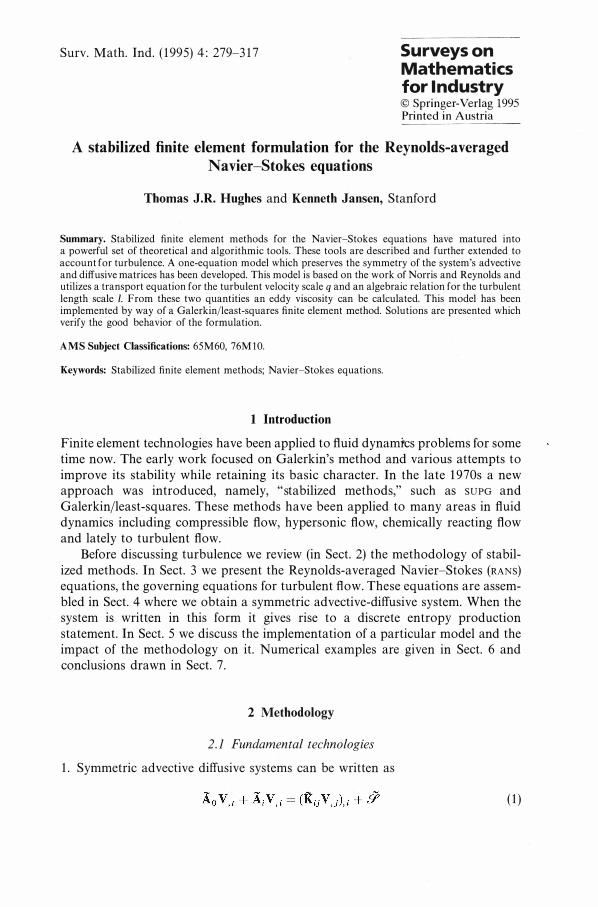
The discontinuity capturing operator was originally developed to control local oscillations in the neighborhood o f shocks for compressible flow, but has been found to be use ful for turbulent flows as well. For example, the turbulent velocity scale takes on values o f the order o f 0.1 when inside the boundary layer but quickly dies off to freestream values o fthe order o f 0.001; see Fig. 7 . This change takes place so quickly that on very coarse meshes (28 x 24 elements in the problem shown in Fig. 7) the method sometimes undershoots to negative values. Note that the GLS operator is o f little help in this situation as the gradient is normal to the streamline or upwind direction. These undershoots are not catastrophic to the global solution but they can easily be avoided without sacrificing accuracy. The effect o f the discontinuity capturing operator can be observed in Fig. 8a. Note that the under shoot is removed with minimal effect on the remainder o f the boundary layer. There is practically no effect in the near wall region where the accuracy o f this variable is crucial to production o f turbulent kinetic energy, fJJ, and eddy viscosity, as seen in Fig. 8b. The effect on skin friction is also seen to be negligible in Fig. 9 .

Implementation o f the discontinuity capturing operator directly followed the work o f Shakib with again changes only arising from the changes to the matrices and variables given in Jansen et al. [15].

0.12

0.10

0.08

0.06

0.04

0.02

0.02 0.04 0.06 0.08 0.10

y

Fig. 7. Undershoot of turbulent velocity scale on coarse mesh (28 x 24 element) flat plate at ReL = 2 x 106


3.0

2.5

2.0 '\ "-

1.5 � + \ '"

1.0 \ \

0.5 \ D-.. ----

0

-0.5 0 0 5 1.0 1.5 2.0 2.5 3.0

a y+ x 10-3

10

+", 1

10 100 1000

b Fig.8. a Turbulent velocity scale profile in wall coordinates on a coarse mesh (28 x 24 element) fiat plate

at ReL = 2 x 106, with and without discontinuity capturing. b A closeup

6 Numerical examples

To verify the formulation and implementation a variety of test problems are studied in this section. These problems range from the simple and well understood flat plate solutions to complex transonic airfoil calculations. Throughout this spectrum of problems the method will be shown to give high quality results, o ften on meshes considered too crude to give reasonable solutions.

All of the problems that will be described in this section were run on a CONvEx -C l computer in double precision (64 bits per floating point), using 2 x 2 Gaussian quadrature for the bilinear elements and 3 -point quadrature for linear triangular elements. Each problem is run using the 1: and vh described in previous


8

7

6

'"' 5

0 \ .-< \ x 4

----..... \.) 3

2

o L-� __ -L __ � __ L-� __ � __ �� __ � __ � __ �� o 0.2 0.4 0 .6 0.8 1 .0 1.2

x

Fig. 9. Effect of discontinuity capturing operator on skin friction, Cf, for a coarse mesh (28 x 24 element) flat plate at ReL = 2 x 106• -- GLS, - - - GLS + vh

sections with linear -in -space constant -in -time elements. They are started either from a freestream or a laminar boundary layer solution. The freestream turbulence is set at

(75)

The following in formation pertains to solver specific in formation that will be most use ful to people familiar with Shakib 's work [24]. It is included to give a general overview o f the numerical experience with these e quations. Local time stepping is used for all problems. For all but the Mach 5 case a CFL o f 10 is used. For the Mach 5 case the CFL number is reduced to 2 as is also done for laminar flow. The GMRES Krylov space is set at 15 with a potential for 4 restarts, but typically 10 or less Krylov vectors are used be fore the algorithm converged to solve the tolerance which is set at 0.1. No element -by -element preconditioning is needed as block diagonal preconditioning was found to be ade quate. A global residual reduction o f 10-4_10-5, combined with steady skin friction, signaled global convergence.

6.1 Flat plate boundary layer: nearly incompressible case

The first problem considered is a nearly incompressible high Reynolds number flow over a flat plate; see Fig. 10 for a complete problem description. By running the compressible code at M = 0.01 we can approximate incompressible flow. The discreti zation used for this calculation is shown in Fig. 11. There are 60 elements normal to the wall with the thinnest element measuring 2.0 x 10-6 meters corres ponding to a y + = 0.5. There are 80 elements in the streamwise direction with a concentration o f points at the sharp tip o f the plate. Here a laminar boundary layer begins its growth along the length o f the plate until at some point the flow undergoes a transition to turbulence. The exact point o f transition depends on

p=p= Ul = UOO

U2 = 0

q= q= o

Tj2 = T,2 = 0


p=p=

Uj = U2 = q = 0 T,2 = 0

Fig. 10. Nearly incompressible flow over a Ilat plate. M = 0.01, ReL = 12 x 106

301

p=p=

x

Fig. 1 1 . Nearly incompressible flow over a flat plate. The discretization shown here contains 80 x 60 elements

many factors . To circumvent this difficulty turbulence modelers o ften compare results based on variables other than x; see White [28] . For example the skin friction C f is usually plotted versus Reo, the Reynolds number based on the momentum thickness, e, which is defined as

(76)

where the superscript e denotes the edge o f the boundary layer . The skin friction is plotted in this fashion in Fig. 12 . The computed turbulent solution follows the Blasius solution, which is exact for laminar flow, until the point o f transition a fter which it quickly joins the empirical branch . This line is a plot o f the KarmanSch onherr correlation

1 2 - = 17 .08 ( lOglO Reo) + 25 .111og1o Reo + 6 .012 Cf

(77)

302 Thomas lR. Hughes and Kenneth Jansen

7

6

5

3 6 9 12 15 18 Rea x 10-3

Fig. 12. Nearly incompressible flow over a flat plate. Coefficient of friction vs. momentum thickness Reynolds number. Theory: -- Blasius, - - - empirical; computation: 0 turbulent, 0 laminar

which was found by examining a large body of experimental results; see [10]. A plot of the laminar skin friction (i.e., no turbulence modeling) is also included in Fig. 12 to validate the accuracy of the compressible code in a nearly incompressible problem. This figure also provides the uninitiated reader with a chance to observe the magnitude of the difference between laminar and turbulent solutions for the same geometry and flow conditions.

The velocity profile of a turbulent boundary layer has been the topic of a great deal of study. The profiles are typically plotted in so called logarithmic wall coordinates where

+ U U =Ut

U = ftw t -P

(78)

where v = /1visc/p is the kinematic viscosity, Ow is the shear stress at the wall; see [28] for background. In these coordinates the boundary layer can be broken into four distinct regions as shown in Fig. 13. Leaving the wall, the first region is the law of the wall region (y+ < 5) where

(79)

Then from 5 < y + < 50 the buffer layer provides a smooth transition to the log law (50 < y + < � 1000, the upper limit depends on the degree to which the boundary

30

25

20

15 +

;l 10

5

0

-5 . 1


u+ = ln�f) + 5.2

K"

I A /AA

iA �.I!f' I Buffer

._._ 1>.-."". layer

Law of the wall

10

Log law

100

Wake region

1000

303

10000

Fig. 13. Nearly incompressible flow over a flat plate. Boundary layer velocity profile description. /::, Computation, Reo = 1 7, 277

+ ;l

25

20

15

1 0

5

o -5

-10

-15 ��--��

.1 10 100 1 000 1 0000

Fig. 14. Nearly incompressible flow over a flat plate. Velocity profiles in logarithmic wall coordinates at various values of momentum thickness Reynolds numbers: li: 1 7,277, 0 13,523, 0 9,543, /::, 5,201.

- . - Wall law, ----- log law

layer has developed) where

(80)

in which % = 0 .41 and the offset B = 5.2. The last region is known as the wake region.

To ascertain the quality of the computed results, the law of the wall (79) and the log law (80) are plotted with the computed solution at various values of Reo in


3.0

2.5

2.0 0

+ \ "" 1.5 � \ \

1.0 q b \ 0.5 \

6 0

0 2 4 6 8 1 0

a y+ x 10-3 10

+"" 1

.1 L-__ �� ____ �� __ � __ �� . 1 10 100 b

Fig. 15. a Nearly incompressible flow over a nat plate. Turbulent velocity scale profiles in wall coordinates at various momentum thickness Reynolds numbers: -6- 1 7, 277, - - z - - 13,523,

- 0 - 9,543, -0- 5,201. b A closeup. Symbols as in a

Fig. 18. The agreement is quite good everywhere but is best for the high values of Reo where the log law region is the largest.

To gain insight into the behavior of the turbulent velocity scale we look to Fig. 15a and b and note that by definition

+ q q = -Ur (81)

As expected q + (and therefore q) is linear near the wall, approaches a maximum near y + = 30, and then returns to the free stream value at the edge of the boundary layer. This steep return to a value near zero can create difficulties for methods which are not strongly diffusive. The problem can be remedied by incorporating the discontinuity capturing operator presented in Shakib [24]. This operator only affects regions with strong gradients, posing no threat to the accuracy in smooth reglOns.


Refinement studies The mesh employed (see Fig. 11) is viewed as moderately fine. The first layer of nodes next to the wall is at y + = 0.5. To study the effect of mesh spacing, the closest point to the wall is allowed to vary while adjusting the remaining nodes to insure a smoothly varying element si ze (i .e., a new mesh is generated for each change of the closest point to the wall). Figure 16a illustrates the effect of near -wall refinement on the velocity profiles. There is very little variation in the results from y + = 0.25 to y + = 2.0, suggesting the solution is normal direction "grid independent ". When the first node is at y + = 5.0, there is some change in the solution but the results are still quite good considering the coarseness of the mesh in the near -wall region. The coefficient of friction is similarly unaffected over this range of refinements as seen in Fig. 16b. Each level of refinement is plotted against the Karman-Sch onherr

30

20

1 0 +

;l

0

-10

-20 .1

a 8

6

4 '" 0 .-<

X 2 ..., C,)

0

0

0

0

0 0

b

. � /'

/ -x - _ . _ - - - - - -

' - ' - ' - ' - ' � ·6 / A' 0

. _ . _ . _ . ¢- ' - /0 D.

. 0 ' ..-0 , D. . _ . - 0- ' - �

. -D. ' ,A'

10 100

y+

• •

X X X <> <> <> 0

3 6 . 9

Reo x 10-3

1 000 1 0000

12 15 18

Fig. 16. Nearly incompressible flow over a flat plate. The effect of varying the normal direction element size a on the boundary layer velocity profile, b on the coefficient of friction. y + : • 5.00, x 200, () 1.00,

D 0.50, 6 0.25


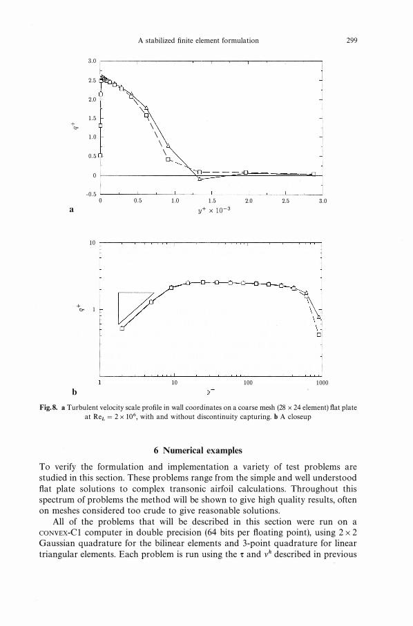
1/11 1/ 1/ 1/1/ 1/11 1/1/ 1/1/1/ 1/1/ III! II 1/ 11 Vii 1/11 1/11 1/11 II II I1I1 I II/II 1/ III/ I1I1 II I1I1 I1I1I1 1/11 1/ I1I1 I1I1 IJ 1/11 II I1I1 I1I1 1/ 111/ 1111 II 1111 l1li11 II I1I1 1/ 111/ II II V I/V 1/ 1/1/ 1/ 1/ VII II 1/1111 II

Fig. 17. Nearly incompressible flow over a flat plate. Triangle discretization

relation given in (77). The laminar branch of the solution is cut from the figure for the sake of clarity.

The quality of the solution on meshes with such coarse near -wall resolution is an important factor when considering the efficiency of a method. Many turbulence models re quire y + ::;; 0.2 to fully resolve the turbulence effects. The benefits are not only limited to a reduction in the number of nodal points (or elements) re quired to resolve a flow. Perhaps more important is the increase in the allowable time step, which is based on the element si ze, resulting in faster convergence to steady state.

Coarse near -wall solution accuracy can be attributed to the choice of q as a turbulent variable. Recall that in Fig. 15b, q was seen to be linear until y + :::::; 5. Likewise the turbulent length scale is also linear near the wall. Thus the scales responsible for turbulence modeling are accurately resolved by linear elements with at least one point at y + ::;; 5. Finally, with the correct turbulence effects, linear elements can also accurately resolve the velocity profile since it too is linear in this region. It should be noted that q may deviate from linearity sooner in more complicated flows thus re quiring more refinement to establish normal direction grid independence.

High aspect -ratio triangle calculation The mesh given in Fig. 11 contains very high aspect -ratio elements. A large portion of the elements have aspect ratios exceeding 4,000, with some approach ing 14,000. It has been proposed that meshes using triangular elements with such high aspect ratios would give poor results. To test this proposal a mesh is generated by subdividing each quadrilateral from Fig. 11 into two triangles. The elements are characteri zed by two angles near 90 ° and one very small angle. The mesh is shown in Fig. 17. This mesh is used to solve the problem described in Fig. 10. The solution is practically identical to the quadrilateral solution as can be observed in Fig. 18a and b. There is actually slightly better agreement in the low -Reynolds number turbulent region. The drawback of this discreti zation is the doubling in the number of elements, resulting in a longer time to solve the problem.

6.2 Flat plate boundary layer: compressible case

The effect of compressibility on turbulence is studied next by repeating the flat plate calculations for various Mach numbers between 0.5 and 5.0. The Mach


7

6

2 � 1 �� 0

0 3 6 9 12 15 18

a Re8 x 10-3

30

25

20

15 + ;3

1 0 0

,Do 5 /

.0 , .0 0 _ _ _ _ 0- -

-5 . 1 1 0 100 1000 1 0000

b y+

Fig. 18. Nearly incompressible flow over a flat plate. a Coefficient of friction, b boundary layer profile calculated with high aspect ratio triangle mesh. a Theory: -- Blasius, - - - empirical; computa

tion: 0 laminar, 0 triangles

5 calculation is generall y considered the limit for this t ype of modeling; see Bradshaw [1] . When the flow is subsonic at the in flow, the boundar y conditions are the same as in Fig . 10 . However, for supersonic in flow conditions the boundar y conditions change to those described in Fig . 19.

Compressibilit y causes a large drop in skin friction over most of the flow as can be seen in Fig. 20. Included with the calculations are two sets of data. The first data clustered around the Mach 5 calculations are values found b y participants in the Collaborative Testing of Turbulence Models (CTTM) stud y at Reo = 10,000; see Bradshaw et al. [2]. The calculation is within the scatter of these results. The second data are values according to the van Driest transformation (described in [ lJ) for the calculated Mach numbers at Reo = 10,000 . It is important to note that the constants described in Table 1 are not modified .

308

p = p=

Ul = UOO U2 = 0

q = q=

T = T=

712 = T,2 = 0

Thomas J.R. Hughes and Kenneth Jansen

p = p=

Boundary layer \ Transition

U, = U2 = q = 0 T,2 = 0

Fig. 19. Supersonic compressible flow over a flat plate. M = M oo :2: 1, ReL = 18 x 106

4.0 J:I I.

3 .5 11

3 .0 Ij � r'·, . � 'b 2.5 I ....... . _ -----<J'--_______ -=

.-< i ' - - ' -x 2 .0

' - ' - ' - ' -<> _ ' _ _ ' _ _ _ . _ _ _ _ . _ .... C,) 1 .5 1 . 0

1 i " . - - - - - - - - - - - - - - - - -1 - - - - - - - - - - - - - - -

0.5 0 0 3 6 9 12 15 18

Reo x 10-3

Fig. 20. Compressible flow over a flat plate. The effect of varying Mach number on the coefficient of friction (-- 0.5, - . - 2.0, - - - 5.0, li: CTTM M = 5, 0 Van Driest)

Bradshaw e t a L [2] sugges t tha t some improvemen t can be made by allowing these cons tan ts to become func tions of the turbulen t Mach number

M =

Ur r C

(82)

where c is the speed of sound . This concep t will be lef t for la ter research as the resul ts shown here are qui te accep table when compared wi th o ther researchers; Bradshaw e t al. [2] .

M = 0.0 1

� p = Poo


Y I� ________

--u--. n_=_o-

Boundary layer \ P = Pex

u = u(y) � ______ ;;;;;;�� ___ � q = q(y) 1m x

1 . 0 U j = U2 = q = 0, T,2 = 0 3 .5

Fig. 21 . Increasingly adverse gradient flow. Refm = 1.7 X 106

6.3 Increasingly adverse pressure gradient

309

A much more challenging problem is presen ted by Samuel and Jouber t [23]; see Fig. 21. The changing area o f this duc t crea tes an increasingly adverse pressure gradien t which in turn drama tically affec ts the boundary layer and the turbulence wi thin. I t should be no ted tha t algebraic models no t specifically tuned for this problem are unable to accura tely solve i t.

The firs t difficul ty wi th a problem like this is se tting the correc t boundary condi tions. Samuel and Jouber t [23] give pressure a t the wall, veloci ty profiles and Reynolds shear s tress profiles be tween 0.855 ::;; x ::;; 3.5. Un for tuna tely the com ple te geome try is no t given. This in forma tion is no t necessary for boundary layer codes which were the me thod o f choice a t the time o f the experimen t. The in forma tion given does no t lend i tsel f to a well -posed problem descrip tion for a Navier -S tokes solver. The bes t tha t can be done is to find the geome try which resul ts in the correc t pressure dis tribu tion (see Fig. 22a) and then s tar t wi th the experimen tal boundary layer a t the in flow be fore curva ture s tar ts (x < 1.0). Con sidering the above uncer tain ty, the coefficien t o f fric tion plo t shown in Fig. 22b is qui te good. The experimen tal da ta are resul ts from using three me thods, Clauser plo ts, Pres ton tube, and a floa ting elemen t. The solu tion s trays significan tly only a t the las t experimen tal poin t, x = 3.38. Examina tion o f o ther researchers ' solu tions made possible by Bradshaw e t al. [2] indica tes tha t this error is no t uncommon, sugges ting a physical difference be tween the modeled problem and the experimen t.

6.4 Transonic flow around a NA CA 0012 airfoil

The nex t problem considered is transonic flow abou t a NA CA 0012 air foil; see Fig. 23 for a comple te problem descrip tion. This flow is sligh tly supersonic near the leading edge o f the upper sur face. The discre ti za tion used to calcula te this flow employs s truc tured quadrila teral elemen ts near the air foil and in the wake while using uns truc tured triangles in the remaining compu ta tional domain; see Fig. 24a for the full domain and Fig. 24b for a closeup o f the body. The regions o f the flow affec ted by turbulence coincide wi th the s truc tured domain thereby simpli fying calcula tion o f dis tance to the wall and boundary layer thickness.


0.6

0.5

0.4

0.3

0" 0.2

0.1

0 11

11 11 11 11 11

-0.1 0 2 3 4

a x

x

<>

o

x <> 0

1 .5 2.0 2.5 3.0 3.5

x

Fig. 22. Increasingly adverse pressure gradient flow. a The coefficient of pressure vs. position in channel. [:, Experiment, -- computation. b The coefficient of friction vs. position in channel. The computation (--) is compared with various methods of experimental measurement. x floating element,

o Clauser plots, 0 Preston tube

Figure 25a shows results for coefficient of pressure, Cp, that are in excellent agreement with ex perimental data of Harris [8]. It is worth noting that the laminar solution to this problem is unsteady and contains regions of massive se paration. The additional diffusivity due to turbulence results in an attached flow des pite the adverse pressure gradient present a fter the suction peak.

The coefficient of friction, Cf , is plotted in Fig. 25b. Ex perimental data are not available for Cf and therefore only a qualitative discussion of the results is a ppro priate. On the to p of the airfoil the skin friction rises and then falls in the first five percent of the chord, consistent with laminar flow. Then at five percent of chord, while the pressure gradient is still strongly favorable, the transition takes place causing a significant rise in the skin friction. Shortly a fter transition the pressure gradient becomes adverse, accelerating the reduction in skin friction over

Re, = 9 X 106

Moo = 0 . 7

a = 1 .490

! •• • • •••• ••• : . • • . • • �


u, = U2 = q = 0

T,;n; = 0

Fig. 23. Transonic flow around a NACA 001 2 airfoil

311

Fig. 24. Transonic flow around a NACA 001 2 airfoil. a Complete domain discretization; 13,177 nodes, 10,480 quadrilaterals, 5,086 triangles. b Structured grid refinement near the air foil

the remaining chord length. The bottom of the airfoil is quite similar but with the transition at ten percent of chord . By contrasting the two surfaces we note the higher peak on the upper surface is associated with the more favorable pressure gradient found there . Similarly, after transition the pressure gradient is more

3 1 2 Thomas J.R. Hughes and Kenneth Jansen

- l . 2

Top -0.8

-0 . 4

CJ" 0

� Bottom 0 . 4

0 . 8

l.2 0 0.2 0.4 0 . 6 0 .8 l . 0 a x

10

8 '" 0 6 .--< Top x

"-, 4 CJ

2

0 0 0 .2 0 .4 0 .6 0 .8 l . 0

10

8 '"' 0 6 .--< Bottom X

4 cJ

2

0 0 0.2 0.4 0 .6 0.8 l . 0 b x

Fig. 25. Transonic flow around a NACA 001 2 airfoil. a Coefficient of pressure (-- computation; 6 , ... experiment), b coefficient o f friction distribution o n the airfoil

adverse on the upper surface causing a more rapid decrease in the coefficient of friction.

6.5 Transonic flow around an RAE 2822 airfoil

The final problem considered in this text is transonic flow around a R A E 2822 airfoil. This flow is similar to the NA CA problem described in Fig. 23 with the following changes. The Reynolds number based on chord is 6.5 x 10 6. The Mach number is 0.725. The angle of attack is 2.92 °.

This problem was chosen as a test case for the "Viscous Transonic Workshop " of 1987. Many solutions are compared in Holst [9]. It was common, among the modelers, to vary the angle of attack to achieve better agreement with the experi mental data of Cook et al. [4]. A closeup of the mesh used to solve this problem is


Fig. 26. Transonic flow around an RAE 2822 airfoil. Closeup of "infinite" domain mesh

given in Fig. 26. Here we have again emplo yed quadrilaterals in the boundar y la yer and triangles elsewhere. In Fig. 27a we present the coefficient of pressure distribu tion along the surface obtained with our method using the experimental angle of attack , 2.92 °. The agreement is quite good with the exception of the shock position. The skin friction on the upper and lower surfaces are presented in Fig. 27b. The solution again compares well with the few data points provided.

The calculation is run on a infinite domain mesh similar to Fig. 24a. The basis for changing the angle of attack is to attempt to correct for the in fluence of the wind tunnel walls , which in this problem are quite close. The boundar y condition for the walls of the wind tunnel is quite di fficult since slats in the wind tunnel are opened to bleed off the blockage effect of the airfoil. In attempting to make their experiment more like an "infinite field " the experiments have created a complicated 3 D problem. Consider the following quote from Garner et al. [6 J :

The boundaries of the ventilated wind tunnel in fluence the flow about the model in a similar manner to the boundaries of the more conventional closed or open -jet tunnel. Indeed , these two t ypes ma y often be regarded as the extreme limits with which the amount of wall ventilation ma y be varied.

This quote , while discouraging in the sense that common 2 D boundar y condi tions cannot replicate the experiment , offers the option of bracketing the experi mental solution with the two extreme limits of a ventilated wind tunnel : an infinite solution and a closed tunnel solution. A closed tunnel solution is obtained if we assume no flow through the walls. This solution is shown in Fig. 28 where the shock is seen to move to the other side of the experimental data. The discreti zation used in this calculation is shown in Fig. 29. This result confirms the quotes contention that ventilated wind tunnels are somewhere between closed tunnels and open -jets , what we call infinite field calculations. It appears that bracketing the

3 1 4 Thomas J.R. Hughes and Kenneth Jansen

-1.6

-1.2

-0.8

-0.4

,-:>"

0.4

0.8

1.2 0 0.2 0.4 0.6 0.8 1 . 0 a x

'"' Top

0 4 .--<

x

G'

0 0 0.2 0.4 0.6 0.8 1.0

6

'" Bottom 0 4 .--<

x

G'

0

b 0 0.2 0.4 0.6 0.8 1.0 x

Fig. 27. Transonic flow around an RAE 2822 airfoil. a Coefficient of pressure (-- computation; 6 , ... experiment), b coefficient o f friction (-- computation, 6 experiment) distribution o n the airfoil

in an "infinite" domain

solution is the best that can be obtained with a 2D solution. The 3D simulation would be very expensive due to the resolution re quirements near the very thin slats.

7 Conclusions

In this text we have seen that the careful analysis built into the new methodology leads to a very robust solver. The analytical tools have been extended to the Reynolds -averaged Navier -Stokes e quations, the governing e quations of turbu lence. The new developments in the method were discussed in the context of a specific model. Simple flat plate flows were used to study model characteristics

A stabilized finite element formulation 3 1 5

- 1 . 6

- 1 . 2

-0 . 8

- 0 . 4

C,)'" 0

0.4

0 .8

1 .2 0 0.2 0 .4 0 . 6 0 .8 1 .0

x

Fig. 28. Transonic flow around an RAE 2822 airfoil in a closed wind tunnel. Coefficient of pressure distribution on the airfoil. Computation (---) performed with a domain bounded by a solid wall. 6 ,

... Experiment

Fig. 29. Transonic flow around an RAE 2822 airfoil. Full domain of closed tunnel mesh

and mesh re quirements. The key findings were :

(i) The q e qu ation is not ill beh aved ne ar a solid w all . (ii) This formul ation is mesh independent when the first point off the w all is at

y+ ::;; 5 (iii) High aspect r atio elements perform well, even when tri angles are used .

More complex flows were also solved to demonstr ate the bro ad applic ability of the model . These flows included fl at pl ate compressible bound ary l ayers, adverse pressure gr adient flows and tr ansonic flow around airfoils. Throughout, good results were obt ained with no adjustment of the modeling const ants .

Acknowledgements

The authors would like to express their appreciation to Peter Bradshaw for insightful guidance into turbulence modeling. We would like to thank Frederic Chalot and Jim Stewart for their mesh

3 1 6 Thomas 1.R. Hughes and Kenneth Jansen

generation help (Jim Stewart provided assistance with the NASA Langley mesh generator used for the RAE 2822 airfoil problem), and Guillermo Hauke, Zdenek Johan, William e. Reynolds and Farzin Shakib for their helpful comments. This work was supported by NASA Langley Research Center under grant NASA-NAG- I -36 1 and the Office of Naval Research under grant 2DJA804.

References

1 . Bradshaw, P. : Compressible turbulent shear layers. Annu. Rev. Fluid Mech. 9 : 33-54 (1 977). 2. Bradshaw, P., Launder, B.E., Lumley, 1.1. : Collaborative testing of turbulence models. AIAA Pap.

9 1 -02 1 5 ( 1991 ). 3. Chalot, F., Hughes, T.J.R., Shakib, F. : Symmetrization of conservation laws with entropy for

high-temperature hypersonic computations. Compu!. Sys!. Eng. 1 : 495-521 ( 1 990). 4. Cook, P.H., McDonald, M.A., Firmin, M.e.P. : Aerofoil RAE 2822 - pressure distributions, and

boundary layer wake measurements. AGARD Advis. Rep. 138 ( 1 979). 5 . Favre, A. : Formulation of the statistical equations of turbulent flows with variable density. In:

Gatski, T.B. (ed.): Studies in turbulence. Springer Berlin Heidelberg, New York Tokyo, pp. 324-34 1 ( 1 992).

6. Garner, H.e., Rogers, E.W.E., Acum, W.E.A., Maskell, E.e.: Subsonic wind tunnel wall corrections. AGARDograph 1 09 : 3 5 1 ( 1966).

7 . Godunov, S.K.: The problem of a generalized solution in the theory of quasilinear equations and in gas dynamics. Russ. Math. Surv. 1 7 : 145-1 56 ( 1 962).

8. Harris, e.D.: Two-dimensional aerodynamics characteristics of the NACA 001 2 airfoil in the Langley 8-foot transonic pressure tunnel. NASA TM 8 1 927 ( 1 98 1 ).

9. Holst, T.L. : Viscous transonic airfoil transonic workshop compendium of results. AIAA Pap. 87-1460 ( 1987).

1 0. Hopkins, E.J., Inouye, M.: An evaluation of theories for predicting turbulent skin friction and heat transfer on flat plates at supersonic and hypersonic Mach numbers. AIAA J. 9 : 993-1003 ( 1 971) .

1 1 . Hughes, TJ.R. , Brooks, A.N. : A multidimensional upwind scheme with no crosswind diffusion. In: Hughes, TJ.R. (ed.): Finite element methods for convection dominated flows. ASME, New York (AMD, vol. 34) ( 1 979).

1 2. Hughes, TJ.R., Franca, L.P., Mallet, M. : A new finite element formulation for computational fluid dynamics: I . Symmetric forms of the compressible Euler and Navier-Stokes equations and the second law of thermodynamics. Compu!. Methods Appl. Mech. Eng. 54 : 223-234 ( 1 986).

13. Hughes, T.J.R., Mallet, M.: A new finite element formulation for computational fluid dynamics: III. The generalized streamline operator for multidimensional advective-diffusive systems. Compu!. Methods Appl. Mech. Eng. 54 : 223-234 ( 1 986).

14. Hughes, TJ.R., Franca, L.P., Hulbert, G.: A new finite element formulation for computational fluid dynamics: VIII. The Galerkin/least-squares method for advective-diffusive equations. Compu!. Methods. Appl. Mech. Eng. 73 : 1 73-189 ( 1 989).

1 5 . Jansen, K., Johan, Z., Hughes, TJ.R.: Implementation of a one-equation turbulence model within a stabilized finite element formulation of a symmetric advective-diffusive system. Compu!. Methods Appl. Mech. Eng. 105 : 405-433 ( 1993).

16 . Johan, Z. : Data parallel finite element techniques for large-scale computational fluid dynamics. Ph.D. thesis, Stanford University, Stanford, Calif., U.S.A. ( 1 992).

1 7. Johan, Z., Hughes, TJ.R., Shakib, F. : A globally convergent matrix-free algorithm for implicit time-marching schemes arising in finite element analysis in fluids. Compu!. Methods Appl. Mech. Eng. 87 : 281-304 ( 199 1 ).

1 8 . Johnson, e., Navert, U., Pitkiiranta, J.: Finite elements methods for linear hyperbolic problems. Compu!. Methods. Appl. Mech. Eng. 45 : 285-3 1 2 ( 1984).

19. Lesaint, P., Raviart, P.: On a finite element method for solving the neutron transport equation. In: de Boor, e. (ed.): Mathematical aspects of finite elements in partial differential equations. Academic Press, New York, pp. 89-123 ( 1974).

20. Mallet, M.: A finite element method for computational fluid dynamics. Ph.D. thesis. Stanford University, Stanford, Calif., U.S.A. ( 1 985) .

21 . Mohammadi, B., Pironneau, 0.: Analysis of the K-e turbulence model, Masson/Wiley, Paris/New York ( 1 994).

22. Norris, L.H., Reynolds, W.e.: Channel flow with a moving wavy boundary. Report FM- IO, Department of Mechanical Engineering, Stanford University, Stanford, Calif. ( 1 975).

23. Samuel, A.E., Joubert, P.N.: A boundary layer developing in an increasingly adverse pressure gradien!. J. Fluid Mech. 66 : 48 1-505 ( 1974).

A stabilized finite element formulation 3 1 7

24. Shakib, F. : Finite element analysis o f the compressible Euler and Navier-Stokes equations. Ph.D. thesis. Stanford University, Stanford, Calif., U.S.A. ( 1 989).

25 . Shakib, F., Hughes, TJ.R., Johan, Z. : A multi-element group preconditioned GM-RES algorithm for nonsymmetric systems arising in finite element analysis. Compu!. Methods App!. Mech. Eng. 75 : 4 1 5-456 ( 1 989).

26. Vandromme, D.: Introduction to turbulence modeling, Von Karman Lecture Series, 1 99 1 -02, Belgium ( 199 1 ).

27. Von Neumann, J., Richtmyer, R.D.: A method for the numerical calculation of hydrodynamic shocks. 1. App!. Phys. 2 1 : 232-237 ( 1950).

28. White, F. : Viscous fluid flow. McGraw-Hill, New York ( 1974).

Authors' address: Dr. Thomas 1.R. Hughes and Kenneth Jansen, Division of Applied Mechanics, Durand Building, Stanford University, Stanford, CA 94305, U.S.A.

Communicated by J. Periaux

Surv. Math. Ind. (1995) 4: 279-317 Surveys on Mathematics...

Documents

Transcript of Surv. Math. Ind. (1995) 4: 279-317 Surveys on Mathematics...