Surfer - sciencesoftware.cz fileUninstalling Surfer 3 A Note about the Documentation 3 Three-Minute...

Surfer®13Powerful contouring, gridding & surface mapping system

Quick Start Guide

Surfer® Quick Start GuideContouring and 3D Surface Mapping

for Scientists and Engineers

Golden Software, LLC809 14th Street, Golden, Colorado 80401-1866, U.S.A.

Phone: 303-279-1021 Fax: 303-279-0909www.GoldenSoftware.com

Surfer® Registration Information

Your Surfer serial number is located on the CD cover or in the email download instructions, depending on how you purchased Surfer.

Register your Surfer serial number online at www.GoldenSoftware.com. This information will not be redistributed.

Registration entitles you to free technical support, free minor updates, and upgrade pricing on future Surfer releases. The serial number is required when you run Surfer the first time, contact technical support, or purchase Surfer upgrades.

For future reference, write your serial number on the line below.

_________________________________

COPYRIGHT NOTICE

Copyright Golden Software, LLC 2015

The Surfer® program is furnished under a license agreement. The Surfer software and quick start guide may be used or copied only in accordance with the terms of the agreement. It is against the law to copy the software or quick start guide on any medium except as specifically allowed in the license agreement. Contents are subject to change without notice.

Surfer is a registered trademark of Golden Software, LLC. All other trademarks are the property of their respective owners.

July 2015

i

Quick Start Guide

Table of ContentsIntroduction to Surfer 1

Who Uses Surfer? 2System Requirements 2Installation Directions 2

Installing Surfer 2Uninstalling Surfer 3

A Note about the Documentation 3Three-Minute Tour 4

Example Surfer Files 4Graticule.srf 4Axes.srf 4

Using Surfer 5Using Scripter 5Example Scripter Files 5

Surfer User Interface 6Changing the Window Layout 8

Displaying Managers 8Auto-Hiding Managers 8Docking Managers 8Customizing Toolbars and Buttons 8

Plot Window 8Menu Commands 9Toolbars 9Status Bar 9Object Manager 9Property Manager 10

Worksheet Window 12Grid Node Editor 12

File Types 13Data Files 13Grid Files 14Base Map Files 14Surfer Files 14

Gridding 14Grid Menu Commands 14Creating a Grid File 14

Gridding Methods 15Grid Line Geometry 15Convex Hull 15Grid Z Limits 16Z Transform 16Breaklines 16Faults 17

Map Types 17Base Map 17

ii

Surfer

Contour Map 18Image Map 18Shaded Relief Map 18Vector Map 18Post Map and Classed Post Map 18Watershed Map 193D Surface Map 193D Wireframe Map 19Viewshed Layer 19

Map Layers 19Coordinate Systems 20

Source Coordinate System - Map Layer 20Target Coordinate System - Map 21Using Coordinate Systems with Multiple Map Layers 21

Tutorial 22Tutorial Lesson Overview 22Using the Tutorial with the Demo Version 22Starting Surfer 23Lesson 1 - Viewing and Creating Data 23

Opening an Existing Data File 23Adding New Data 24Creating a New Data File 24Saving the Data File 25

Lesson 2 - Creating a Grid File 25Lesson 3 - Creating a Contour Map 27

Changing Contour Levels 28Changing Contour Line Properties 28Changing Contour Fill Properties 29Setting Advanced Contour Level Properties 30Adding, Deleting, and Moving Contour Labels 32

Lesson 4 - Modifying an Axis 32Adding an Axis Title 33Changing the Tick Label Properties 33

Lesson 5 - Posting Data Points and Working with Layers 34Adding a Post Map Layer 34Editing the Post Map 35Adding Labels to the Post Map 36Moving Individual Post Map Labels 36

Lesson 6 - Creating a Profile 37Lesson 7 - Saving a Map 37Lesson 8 - Creating a 3D Surface Map 38

Creating a 3D Surface Map 38Adding a Mesh 39Changing the 3D Surface Layer Colors 39Adding a Map Layer 40

Lesson 9 - Adding Transparency, Color Scales, and Titles 40Creating a Filled Contour Map 41

iii

Quick Start Guide

Applying Opacity 41Adding and Editing a Color Scale Bar 42Downloading an Online Base Map Layer 42Adding a Map Title 43

Lesson 10 - Creating Maps from Different Coordinate Systems 43Creating the First Map 44Creating a New Map and Assigning a Coordinate System 44Setting the Target Coordinate System 45Changing the Axis Label Format 45

Printing the Online Help 46Getting Help 47

Internet Resources 47Technical Support 48Contact Information 48

Index 49

Surfer

1

Quick Start Guide

Introduction to SurferWelcome to Surfer, a powerful contouring, gridding, and surface mapping package for scientists, engineers, educators, or anyone who needs to generate maps quickly and easily. Producing publication quality maps has never been quicker or easier. Adding multiple map layers and objects, customizing the map display, and annotating with text creates attractive and informative maps. Virtually all aspects of your maps can be customized to produce the exact presentation you want.

Surfer is a grid-based mapping program that interpolates irregularly spaced XYZ data into a regularly spaced grid. Grids may also be imported or downloaded from other sources, such as the United States Geological Survey (USGS). The grid is used to produce different types of maps including contour, vector, image, shaded relief, watershed, viewshed, 3D surface, and 3D wireframe maps. Produce the map that best represents your data with Surfer’s many gridding and mapping options.

An extensive suite of gridding methods is available in Surfer. The variety of available methods provides different interpretations of your data and allows you to choose the most appropriate method for your needs. In addition, data metrics present information about your gridded data. Surface area, projected planar area, and volumetric calculations can be performed quickly in Surfer.

The grid files can be edited, combined, filtered, sliced, queried, and mathematically transformed. For example, grids can be sliced to create cross-sectional profiles, or you can create an isopach map from two grid files. You will need the original surface grid file and the surface grid file after a volume of material was removed. Use the Grid | Math command to subtract the two surfaces to create an isopach map. The resulting map displays how much material has been removed in all areas.

The ScripterTM program, included with Surfer, is useful in creating, editing, and running script files that automate Surfer procedures. By writing and running script files, simple mundane tasks or complex system integration tasks can be performed precisely and repetitively without direct interaction. Surfer also supports ActiveX Automation using any compatible client, such as Visual BASIC. These two automation capabilities allow Surfer to be used as a data visualization and map generation post-processor for any scientific modeling system.

New Features in Surfer 13 are summarized:• Online at: www.GoldenSoftware.com/products/surfer#what-s-new• In the program, click Help | Contents and click on the New Features page in the

Introduction book

2

Surfer

Who Uses Surfer?People from many different disciplines use Surfer. Since 1984, over 100,000 scientists and engineers worldwide have discovered Surfer’s power and simplicity. Surfer’s outstanding gridding and contouring capabilities have made Surfer the software of choice for working with XYZ data. Over the years, Surfer users have included hydrologists, engineers, geologists, archeologists, oceanographers, biologists, foresters, geophysicists, medical researchers, climatologists, educators, students, and more! Anyone wanting to visualize their XYZ data with striking clarity and accuracy will benefit from Surfer’s powerful features!

System RequirementsThe following are the minimum system requirements for Surfer:• Windows XP SP2 or SP3, Vista, 7, 8 (excluding RT), and higher• 512MB RAM minimum for simple data sets, 1GB RAM recommended• At least 500MB of free hard disk space• 1024 x 768 or higher monitor resolution with a minimum 16-bit color depth

Installation DirectionsInstalling Surfer requires logging onto the computer with an account that has Administrator rights. Golden Software does not recommend installing Surfer 13 over any previous versions of Surfer. Surfer 13 can coexist with older versions (e.g. Surfer 12) as long as both versions are installed in different directories. By default the program installation directories are different. For detailed installation directions see the Readme.rtf file.

Installing SurferTo install Surfer from a CD,1. Insert the Surfer CD into the CD-ROM drive. The install program automatically

begins on most computers. If the installation does not begin automatically, double-click on the Autorun.exe file located on the Surfer CD.

2. Choose Install Surfer from the Surfer Auto Setup dialog to begin the installation.

To install Surfer from a download,1. Download Surfer according to the emailed directions you received.2. Double-click on the downloaded file to begin the installation process.

3

Quick Start Guide

Updating SurferTo update Surfer, open the program and click the Help | Check for Update command. The Internet Update program will check Golden Software’s servers for any free updates. If there is an update for your version of Surfer (e.g. Surfer 13.0 to Surfer 13.1), you will be prompted to download the update.

Uninstalling SurferWindows XP: To uninstall Surfer, go to the Control Panel and double-click Add/Remove Programs. Select Surfer 13 from the list of installed applications. Click the Remove button to uninstall Surfer 13.

Windows Vista: To uninstall Surfer when using the Regular Control Panel Home, click the Uninstall a program link. Select Surfer 13 from the list of installed applications. Click the Uninstall button to uninstall Surfer 13.

To uninstall Surfer when using the Classic View Control Panel, double-click Programs and Features. Select Surfer 13 from the list of installed applications. Click the Uninstall button to uninstall Surfer 13.

Windows 7: To uninstall Surfer go to the Control Panel and click the Uninstall a program link. Select Surfer 13 from the list of installed applications. Click the Uninstall button to uninstall Surfer 13.

Windows 8: From the Start screen, right-click the Surfer 13 tile and click the Uninstall button at the bottom of the screen. Alternatively, right-click anywhere on the Start screen and click All apps at the bottom of the screen. Right-click the Surfer 13 tile and click Uninstall at the bottom of the screen.

A Note about the DocumentationThe Surfer documentation includes this quick start guide and the online help. Use the Help | Contents command in the program to access the detailed online help. Information about each command and feature of Surfer is included in the online help. In the event the information you need cannot be located in the online help, other sources of Surfer help include our support forum, knowledge base, FAQs, newsletters, blog, and contacting our technical support engineers. You can purchase the full PDF user’s guide that includes all of the documentation for the program. This PDF user’s guide can be printed by the user, if desired. The guide can be purchased on the Golden Software website at www.GoldenSoftware.com.

4

Surfer

Various font styles are used throughout the Surfer documentation. Bold text indicates menu commands, dialog names, window names, and page names. Italic text indicates items within a manager or dialog such as group names, options, and field names. For example, the Save As dialog contains a Save as type drop-down list. Bold and italic text occasionally may be used for emphasis.

In addition, menu commands appear as File | Open. This means, “click the File menu at the top of the Surfer window and click the Open command on the File menu list.” The first word is the menu name, followed by the command within the menu list.

Three-Minute TourWe have included several example files so that you can quickly see some of Surfer’s capabilities. Only a few example files are discussed here, and these examples do not include all of Surfer’s many map types and features. The Object Manager is a good source of information as to what is included in each file.

Example Surfer FilesTo view the example Surfer files,1. Open Surfer.2. Click the File | Open command.3. Click on an .SRF file located in the Samples

folder. By default the Surfer Samples folder is located in C:\Program Files\Golden Software\Surfer 13\Samples.

4. Click Open and the file opens.

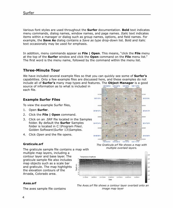
Graticule.srf

The graticule sample file contains a map with multiple map layers, including a contour layer and base layer. The graticule sample file also includes map objects such as a scale bar and graticule. The map highlights the elevation contours of the Arvada, Colorado area.

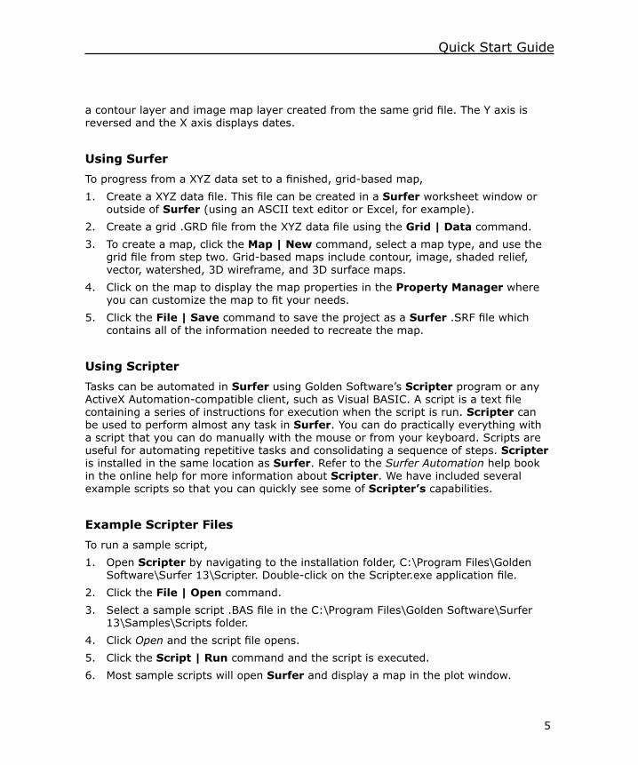
Axes.srf

The axes sample file contains

The Graticule.srf file shows a map with multiple overlaid layers.

The Axes.srf file shows a contour layer overlaid onto an image map layer

5

Quick Start Guide

a contour layer and image map layer created from the same grid file. The Y axis is reversed and the X axis displays dates.

Using SurferTo progress from a XYZ data set to a finished, grid-based map,1. Create a XYZ data file. This file can be created in a Surfer worksheet window or

outside of Surfer (using an ASCII text editor or Excel, for example).2. Create a grid .GRD file from the XYZ data file using the Grid | Data command.3. To create a map, click the Map | New command, select a map type, and use the

grid file from step two. Grid-based maps include contour, image, shaded relief, vector, watershed, 3D wireframe, and 3D surface maps.

4. Click on the map to display the map properties in the Property Manager where you can customize the map to fit your needs.

5. Click the File | Save command to save the project as a Surfer .SRF file which contains all of the information needed to recreate the map.

Using ScripterTasks can be automated in Surfer using Golden Software’s Scripter program or any ActiveX Automation-compatible client, such as Visual BASIC. A script is a text file containing a series of instructions for execution when the script is run. Scripter can be used to perform almost any task in Surfer. You can do practically everything with a script that you can do manually with the mouse or from your keyboard. Scripts are useful for automating repetitive tasks and consolidating a sequence of steps. Scripter is installed in the same location as Surfer. Refer to the Surfer Automation help book in the online help for more information about Scripter. We have included several example scripts so that you can quickly see some of Scripter’s capabilities.

Example Scripter FilesTo run a sample script,1. Open Scripter by navigating to the installation folder, C:\Program Files\Golden

Software\Surfer 13\Scripter. Double-click on the Scripter.exe application file.2. Click the File | Open command.3. Select a sample script .BAS file in the C:\Program Files\Golden Software\Surfer

13\Samples\Scripts folder.4. Click Open and the script file opens.5. Click the Script | Run command and the script is executed.6. Most sample scripts will open Surfer and display a map in the plot window.

6

Surfer

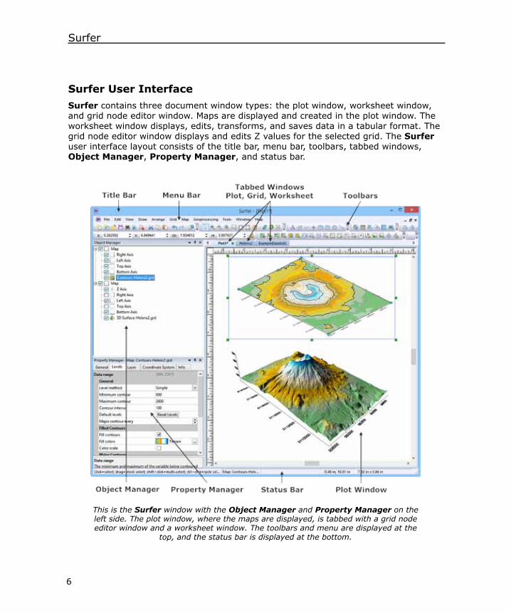
Surfer User InterfaceSurfer contains three document window types: the plot window, worksheet window, and grid node editor window. Maps are displayed and created in the plot window. The worksheet window displays, edits, transforms, and saves data in a tabular format. The grid node editor window displays and edits Z values for the selected grid. The Surfer user interface layout consists of the title bar, menu bar, toolbars, tabbed windows, Object Manager, Property Manager, and status bar.

This is the Surfer window with the Object Manager and Property Manager on the left side. The plot window, where the maps are displayed, is tabbed with a grid node editor window and a worksheet window. The toolbars and menu are displayed at the

top, and the status bar is displayed at the bottom.

7

Quick Start Guide

The following table summarized the function of each component of the Surfer layout.

Component Name

Component Function

Title Bar The title bar displays the program name plus the saved Surfer .SRF file name, if any. An asterisk (*) after the file name indicates the file has been modified since it was last saved.

Menu Bar The menu bar contains the commands used to run Surfer.Toolbars The toolbars contain Surfer tool buttons, which are shortcuts to

menu commands. Move the cursor over each button to display a tool tip describing the command. Toolbars can be customized with the Tools | Customize command. Toolbars can be docked or floating.

Tabbed Windows Multiple plot windows, worksheet windows, and grid windows can be displayed as tabs. Click on the tab to display that window.

Object Manager The Object Manager contains a hierarchical list of the objects in a Surfer plot window. These objects can be selected, added, arranged, edited, and renamed in the Object Manager. The Object Manager is initially docked on the left side above the Property Manager. Changes made in the Object Manager are immediately reflected in the plot window. The Object Manager can be dragged and placed at any location on the screen.

Property Manager The Property Manager allows you to edit any of the properties of a selected object. Multiple objects can be edited at the same time by selecting all of the objects and changing the shared properties. Changes made in the Property Manager are immediately reflected in the plot window.

Status Bar The status bar displays information about the activity in Surfer. The status bar is divided into five sections. The sections display basic plot commands and descriptions, the name of the selected object, the cursor map coordinates, the cursor page coordinates, and the dimensions of the selected object.

The status bar also indicates the progress of a procedure, such as gridding. The percent of completion and time remaining are displayed.

8

Surfer

Changing the Window LayoutThe windows, toolbars, managers, and menu bar display in a docked view by default; however, they can also be displayed as floating windows. The visibility, size, and position of each item may also be changed. Refer to the Changing the Windows Layout topic in the online help for more information on layout options.

Displaying Managers

Click the appropriate View | Managers command to display the various managers. The manager is visible when the button is pressed. The manager is hidden when the button is not pressed.

Auto-Hiding Managers

You can increase the view window space by minimizing the managers. To hide the manager, click the button in the upper right corner of the manager when the manager is docked. When the manager is hidden, place the cursor directly over the tab to display the manager again. Click the button to return the manager to a docked position.

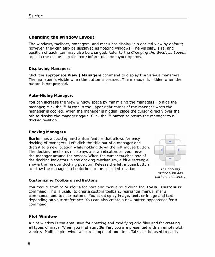
Docking Managers

Surfer has a docking mechanism feature that allows for easy docking of managers. Left-click the title bar of a manager and drag it to a new location while holding down the left mouse button. The docking mechanism displays arrow indicators as you move the manager around the screen. When the cursor touches one of the docking indicators in the docking mechanism, a blue rectangle shows the window docking position. Release the left mouse button to allow the manager to be docked in the specified location.

Customizing Toolbars and Buttons

You may customize Surfer’s toolbars and menus by clicking the Tools | Customize command. This is useful to create custom toolbars, rearrange menus, menu commands, and toolbar buttons. You can display image, text, or image and text depending on your preference. You can also create a new button appearance for a command.

Plot WindowA plot window is the area used for creating and modifying grid files and for creating all types of maps. When you first start Surfer, you are presented with an empty plot window. Multiple plot windows can be open at one time. Tabs can be used to easily

The docking mechanism has

docking indicators.

9

Quick Start Guide

move between multiple plot windows. If you need to change the display of tabs click the Tools | Options command. Select User Interface on the left side of the dialog. Set the MDI tab style on the right side. Setting this value to None turns the display of tabs off.

Menu Commands

The menus contain commands that allow you to add, edit, and control the objects on the plot window page. See the Introduction help book in the online help for the Menu Commands help book that detail the various menu commands.

Toolbars

Toolbars display buttons that represent menu commands for easier access. Use the View | Toolbars commands to show or hide a toolbar. A check mark is displayed next to visible toolbars. Hold the cursor over any button on the toolbar to display the function of the button as a screen tip. A more detailed description is displayed in the status bar at the bottom of the window.

Status Bar

The status bar is located at the bottom of the window. Use the View | Status Bar command to show or hide the status bar. The status bar displays information about the current command or activity in Surfer. The status bar is divided into five sections. The left section displays information about the selected command or item in the Property Manager. The second section shows the selected object name. The middle section shows the cursor coordinates in map units, if the cursor is placed above a map. The fourth section shows the cursor coordinates in page units of inches or centimeters. The right section displays the dimensions of the selected object.

Object Manager

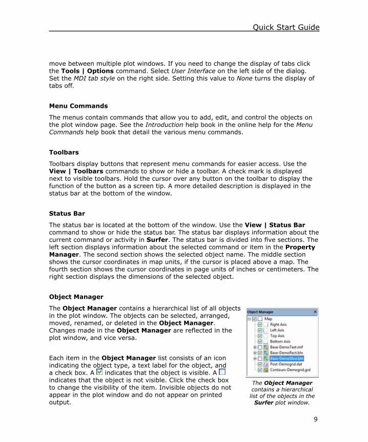
The Object Manager contains a hierarchical list of all objects in the plot window. The objects can be selected, arranged, moved, renamed, or deleted in the Object Manager. Changes made in the Object Manager are reflected in the plot window, and vice versa.

Each item in the Object Manager list consists of an icon indicating the object type, a text label for the object, and a check box. A indicates that the object is visible. A indicates that the object is not visible. Click the check box to change the visibility of the item. Invisible objects do not appear in the plot window and do not appear on printed output.

The Object Manager contains a hierarchical list of the objects in the

Surfer plot window.

10

Surfer

If an object contains sub-objects, a or button displays to the left of the object name. Click on the or button to expand or collapse the list. For example, a map object contains a map type, such as a contour layer, and normally four axes. The Map can contain many other objects. To expand the Map tree to see the axes and map layers, click on the button next to Map. To collapse the Map tree, click on the button next to Map.

Click on the object name to select an object and display its properties in the Property Manager. The selection handles in the plot window change to indicate the selected item and the status bar displays the name of the selected object. To select multiple objects in the Object Manager, hold down the CTRL key and click on each object.

To edit an object’s text ID, select the object and then click again on the selected item (two slow clicks) to edit the text ID associated with an object. You must allow enough time between the two clicks so it is not interpreted as a double-click. Enter the new name into the box. Alternatively, you can right-click on an object name and select Rename Object, click the Edit | Rename Object command, or press F2 on the keyboard. Enter an ID in the Rename Object dialog and click OK.

To change the display order of the objects with the mouse, select an object and drag it to a new position in the list above or below an object at the same level in the tree. The cursor changes to a black arrow if the object can be moved to the cursor location or a red circle with a diagonal line if the object cannot be moved to the indicated location. For example, a 3D surface map layer cannot be moved to a map that contains a 3D wireframe layer but can be moved into a map that only contains a contour map layer. In addition to dragging objects in the Object Manager, the order can be changed with the Arrange | Order Objects commands.

To delete an object, select the object and press the DELETE key. To move a map layer from one map to a new map, click on the map layer and click Map | Break Apart Layer. Alternatively right-click on the map layer and select Break Apart Layer.

Property Manager

The Property Manager allows you to edit the properties of an object, such as a contour map or axis. The Property Manager contains a list of all properties for the selected object. The Property Manager can be left open so that the properties of the selected object are always visible. When the Property Manager is hidden or closed, double-clicking on an object opens the Property Manager with the properties for the selected object displayed. Information about the object properties is located in the online help.

11

Quick Start Guide

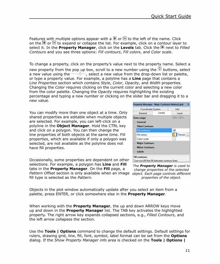
Features with multiple options appear with a or to the left of the name. Click on the or to expand or collapse the list. For example, click on a contour layer to select it. In the Property Manager, click on the Levels tab. Click the next to Filled Contours and you see three options: Fill contours, Fill colors, and Color scale.

To change a property, click on the property’s value next to the property name. Select a new property from the pop up box, scroll to a new number using the buttons, select a new value using the , select a new value from the drop-down list or palette, or type a property value. For example, a polyline has a Line page that contains a Line Properties section which contains Style, Color, Opacity, and Width properties. Changing the Color requires clicking on the current color and selecting a new color from the color palette. Changing the Opacity requires highlighting the existing percentage and typing a new number or clicking on the slider bar and dragging it to a new value.

You can modify more than one object at a time. Only shared properties are editable when multiple objects are selected. For example, you can left-click on a polyline in the Object Manager. Hold the CTRL key and click on a polygon. You can then change the line properties of both objects at the same time. Fill properties, which are available if only a polygon was selected, are not available as the polyline does not have fill properties.

Occasionally, some properties are dependent on other selections. For example, a polygon has Line and Fill tabs in the Property Manager. On the Fill page, a Pattern Offset section is only available when an image fill type is selected as the Pattern.

Objects in the plot window automatically update after you select an item from a palette, press ENTER, or click somewhere else in the Property Manager.

When working with the Property Manager, the up and down ARROW keys move up and down in the Property Manager list. The TAB key activates the highlighted property. The right arrow key expands collapsed sections, e.g., Filled Contours, and the left arrow collapses the section.

Use the Tools | Options command to change the default settings. Default settings for rulers, drawing grid, line, fill, font, symbol, label format can be set from the Options dialog. If the Show Property Manager info area is checked on the Tools | Options |

The Property Manager is used to change properties of the selected

object. Each page controls different properties of the object.

12

Surfer

User Interface page, a short help statement for each selected command will appear in the Property Manager.

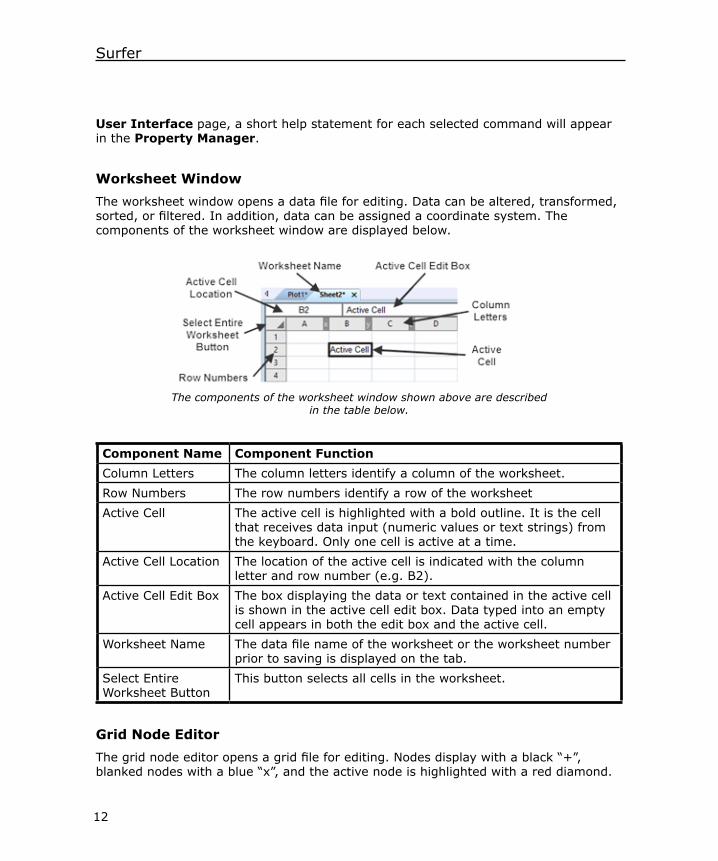
Worksheet WindowThe worksheet window opens a data file for editing. Data can be altered, transformed, sorted, or filtered. In addition, data can be assigned a coordinate system. The components of the worksheet window are displayed below.

Component Name Component FunctionColumn Letters The column letters identify a column of the worksheet.Row Numbers The row numbers identify a row of the worksheetActive Cell The active cell is highlighted with a bold outline. It is the cell

that receives data input (numeric values or text strings) from the keyboard. Only one cell is active at a time.

Active Cell Location The location of the active cell is indicated with the column letter and row number (e.g. B2).

Active Cell Edit Box The box displaying the data or text contained in the active cell is shown in the active cell edit box. Data typed into an empty cell appears in both the edit box and the active cell.

Worksheet Name The data file name of the worksheet or the worksheet number prior to saving is displayed on the tab.

Select Entire Worksheet Button

This button selects all cells in the worksheet.

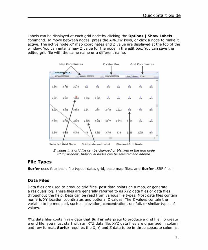
Grid Node EditorThe grid node editor opens a grid file for editing. Nodes display with a black “+”, blanked nodes with a blue “x”, and the active node is highlighted with a red diamond.

The components of the worksheet window shown above are described in the table below.

13

Quick Start Guide

Labels can be displayed at each grid node by clicking the Options | Show Labels command. To move between nodes, press the ARROW keys, or click a node to make it active. The active node XY map coordinates and Z value are displayed at the top of the window. You can enter a new Z value for the node in the edit box. You can save the edited grid file with the same name or a different name.

File TypesSurfer uses four basic file types: data, grid, base map files, and Surfer .SRF files.

Data FilesData files are used to produce grid files, post data points on a map, or generate a residuals log. These files are generally referred to as XYZ data files or data files throughout the help. Data can be read from various file types. Most data files contain numeric XY location coordinates and optional Z values. The Z values contain the variable to be modeled, such as elevation, concentration, rainfall, or similar types of values.

XYZ data files contain raw data that Surfer interprets to produce a grid file. To create a grid file, you must start with an XYZ data file. XYZ data files are organized in column and row format. Surfer requires the X, Y, and Z data to be in three separate columns.

Z values in a grid file can be changed or blanked in the grid node editor window. Individual nodes can be selected and altered.

14

Surfer

Grid FilesGrid files produce several different types of grid-based maps, are used to perform grid calculations, and to carry out grid operations. Grid files are a regularly spaced rectangular array of Z values in columns and rows. Grid files can be created in Surfer using the Grid | Data command or can be imported from a wide variety of sources.

Base Map FilesBase map files contain XY location data such as aerial photography, state boundaries, rivers, or point locations. Base map files can be used to create layers overlaid on other map types, or to specify the limits for blanking, faults, breaklines, or slice calculations Base map files can be created from a wide variety of vector and image formats.

Surfer FilesSurfer .SRF files preserve all the objects and object settings contained in a plot window. Maps, grid files, base map files, and data files are all included in the .SRF.

GriddingGridding is the process of taking irregularly spaced XYZ data and generating a regularly spaced grid of Z values at each grid node by interpolating or extrapolating the data values. In addition to gridding data, Surfer can also use a variety of other grid files directly. For a list of these, refer to the online help.

A grid is a rectangular region comprised of evenly spaced rows and columns. The intersection of a row and column is called a grid node. Rows contain grid nodes with the same Y coordinate. Columns contain grid nodes with the same X coordinate. Contour, image, shaded relief, vector, viewshed, watershed, 3D surface, and 3D wireframe map layers all require grids in Surfer.

Grid Menu CommandsThere are many ways to manipulate grid files in Surfer. The Grid menu contains commands used to blank, convert, create, extract, filter, mosaic, slice, smooth, and transform grid files. In addition, volume calculations, variogram generation, calculus operations, cross section creation, and residual calculations can be performed using the commands under the Grid menu.

Creating a Grid FileClick the Grid | Data command to grid data in Surfer. With this command, you can specify the parameters for the particular gridding method and the extents of the grid.

15

Quick Start Guide

The gridding methods define the way in which the XYZ data are interpolated when producing a grid file.

Gridding Methods

Gridding the data produces a regularly spaced, rectangular array of Z values from irregularly spaced XYZ data. The term irregularly spaced means that the points follow no particular pattern over the extent of the map, so there are many holes where data are missing. Gridding fills in these holes by extrapolating or interpolating Z values at those locations where no data exists. The gridding method determines the mathematical algorithms used to compute the Z value at each grid node. Each method results in a different representation of your data. It is advantageous to test each method with a typical data set to determine the gridding method that provides you with the most satisfying interpretation of your data.

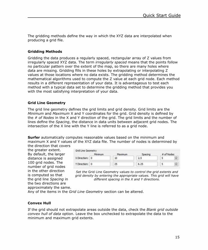
Grid Line Geometry

The grid line geometry defines the grid limits and grid density. Grid limits are the Minimum and Maximum X and Y coordinates for the grid. Grid density is defined by the # of Nodes in the X and Y direction of the grid. The grid limits and the number of lines define the Spacing, the distance in data units between adjacent grid nodes. The intersection of the X line with the Y line is referred to as a grid node.

Surfer automatically computes reasonable values based on the minimum and maximum X and Y values of the XYZ data file. The number of nodes is determined by the direction that covers the greater extent. By default, the larger distance is assigned 100 grid nodes. The number of grid nodes in the other direction is computed so that the grid line Spacing in the two directions are approximately the same. Any of the items in the Grid Line Geometry section can be altered.

Convex Hull

If the grid should not extrapolate areas outside the data, check the Blank grid outside convex hull of data option. Leave the box unchecked to extrapolate the data to the minimum and maximum grid extents.

Set the Grid Line Geometry values to control the grid extents and grid density by entering the appropriate values. This grid will have

different spacing in the X and Y directions.

16

Surfer

The Inflate convex hull by option expands or contracts the convex hull. When set to zero, the boundary connects the outside data points exactly. When set to a positive value, the area blanked is moved outside the convex hull boundary by the number of map units specified. When set to a negative value, the area blanked is moved inside the convex hull boundary by the number of map units specified. Values are in horizontal (X) map units. When the value is set to a large positive value, the contours will extend all the way to the minimum and maximum X and Y limits of the grid. When the value is set to a large negative value, the entire grid will be blanked, resulting in no grid file being created.

Grid Z Limits

Some gridding methods result in values smaller than the data minimum or larger than the data maximum. For example, negative values cannot exist for many physical properties, such as concentration, but a grid created with the Kriging gridding method may include negative Z values. If the grid Z values should be limited to a minimum value, such as 0 or the data minimum, click the current selection next to Minimum and select Data min or Custom. Click the current selection next to Maximum and select Data max or Custom to limit the grid Z values to a maximum value. Any interpolated value outside the specified range will be automatically changed to the user-defined limit.

Z Transform

The Z Transform option changes how the Z values are gridded. Linear uses the Z values in the worksheet for gridding. No transformation is applied to the Z values. The Log, save as log takes the log (base 10) of the Z values and uses the log value for gridding. The grid is then saved with the log (base 10) values. The Log, save as linear takes the log (base 10) of the Z values and uses the log value for gridding. The grid is then converted back to the linear Z values by taking the antilog of the gridded results. The grid is then saved with the linear values.

Breaklines

Breaklines are used when gridding to show discontinuity in the grid. A breakline is a three-dimensional .BLN boundary file that defines a line with X, Y, and Z values at each vertex. When the gridding algorithm sees a breakline, it calculates the Z value of the nearest point along the breakline, and uses that value in combination with nearby data points to calculate the grid node value. Surfer uses linear interpolation to determine the values between breakline vertices when gridding. Breaklines are not barriers to information flow, and the gridding algorithm can cross the breakline to use a point on the other side of the breakline. If a point lies on the breakline, the value of the breakline takes precedence over the point. Breakline applications include defining streamlines, ridges, and other breaks in the slope.

17

Quick Start Guide

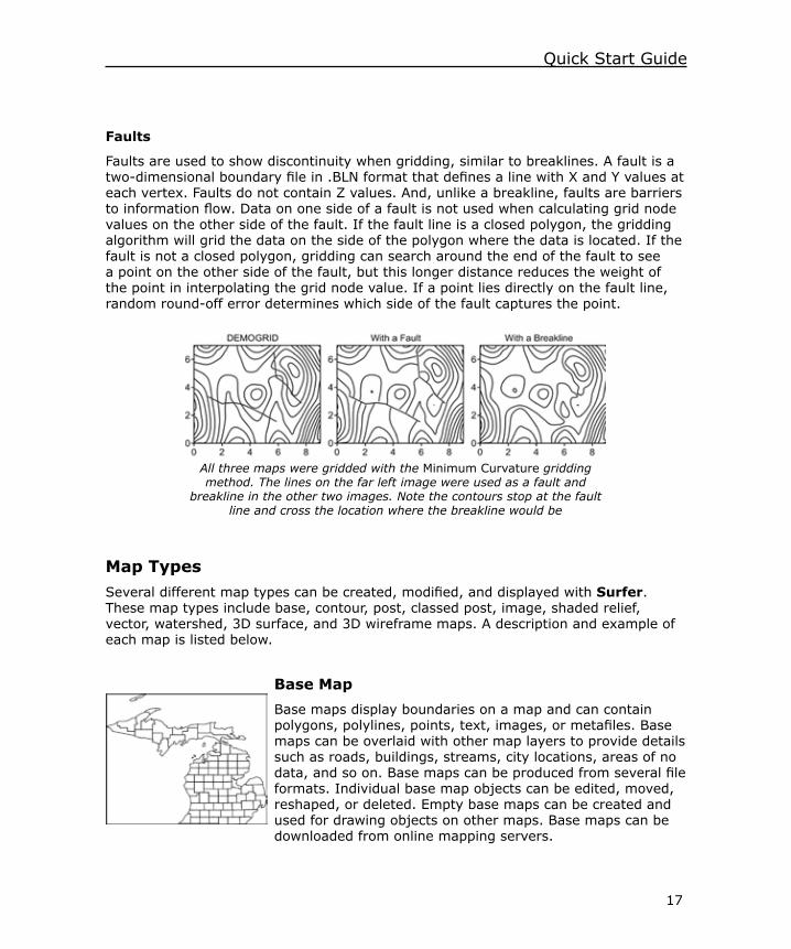
Faults

Faults are used to show discontinuity when gridding, similar to breaklines. A fault is a two-dimensional boundary file in .BLN format that defines a line with X and Y values at each vertex. Faults do not contain Z values. And, unlike a breakline, faults are barriers to information flow. Data on one side of a fault is not used when calculating grid node values on the other side of the fault. If the fault line is a closed polygon, the gridding algorithm will grid the data on the side of the polygon where the data is located. If the fault is not a closed polygon, gridding can search around the end of the fault to see a point on the other side of the fault, but this longer distance reduces the weight of the point in interpolating the grid node value. If a point lies directly on the fault line, random round-off error determines which side of the fault captures the point.

Map TypesSeveral different map types can be created, modified, and displayed with Surfer. These map types include base, contour, post, classed post, image, shaded relief, vector, watershed, 3D surface, and 3D wireframe maps. A description and example of each map is listed below.

Base MapBase maps display boundaries on a map and can contain polygons, polylines, points, text, images, or metafiles. Base maps can be overlaid with other map layers to provide details such as roads, buildings, streams, city locations, areas of no data, and so on. Base maps can be produced from several file formats. Individual base map objects can be edited, moved, reshaped, or deleted. Empty base maps can be created and used for drawing objects on other maps. Base maps can be downloaded from online mapping servers.

All three maps were gridded with the Minimum Curvature gridding method. The lines on the far left image were used as a fault and

breakline in the other two images. Note the contours stop at the fault line and cross the location where the breakline would be

18

Surfer

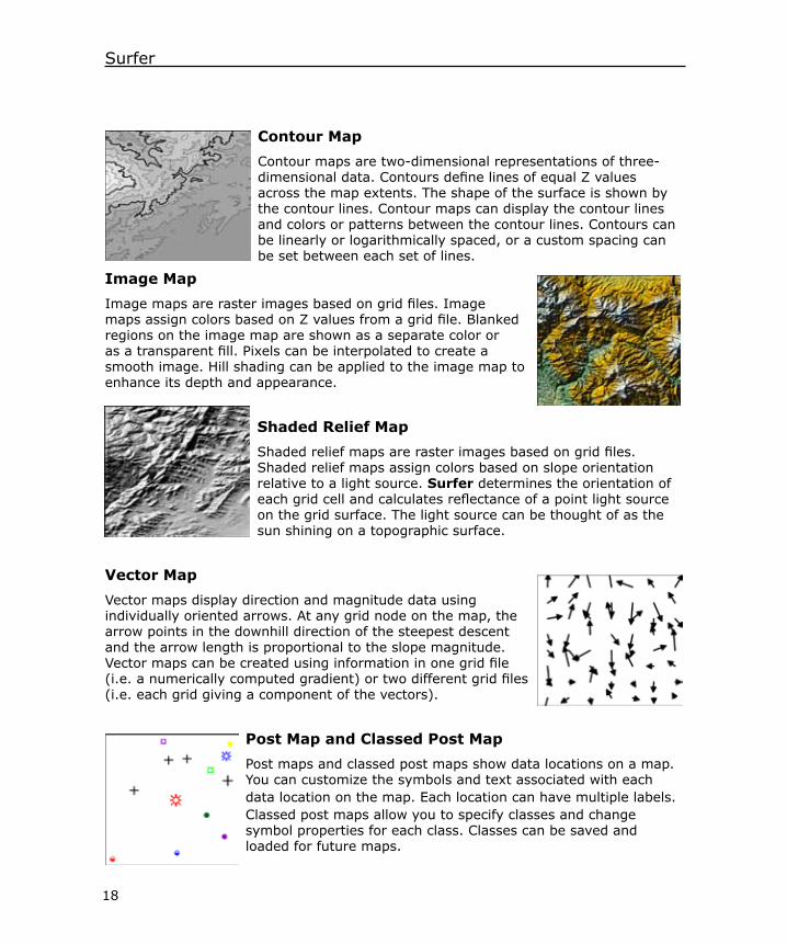
Contour MapContour maps are two-dimensional representations of three-dimensional data. Contours define lines of equal Z values across the map extents. The shape of the surface is shown by the contour lines. Contour maps can display the contour lines and colors or patterns between the contour lines. Contours can be linearly or logarithmically spaced, or a custom spacing can be set between each set of lines.

Image MapImage maps are raster images based on grid files. Image maps assign colors based on Z values from a grid file. Blanked regions on the image map are shown as a separate color or as a transparent fill. Pixels can be interpolated to create a smooth image. Hill shading can be applied to the image map to enhance its depth and appearance.

Shaded Relief MapShaded relief maps are raster images based on grid files. Shaded relief maps assign colors based on slope orientation relative to a light source. Surfer determines the orientation of each grid cell and calculates reflectance of a point light source on the grid surface. The light source can be thought of as the sun shining on a topographic surface.

Vector MapVector maps display direction and magnitude data using individually oriented arrows. At any grid node on the map, the arrow points in the downhill direction of the steepest descent and the arrow length is proportional to the slope magnitude. Vector maps can be created using information in one grid file (i.e. a numerically computed gradient) or two different grid files (i.e. each grid giving a component of the vectors).

Post Map and Classed Post MapPost maps and classed post maps show data locations on a map. You can customize the symbols and text associated with each data location on the map. Each location can have multiple labels. Classed post maps allow you to specify classes and change symbol properties for each class. Classes can be saved and loaded for future maps.

19

Quick Start Guide

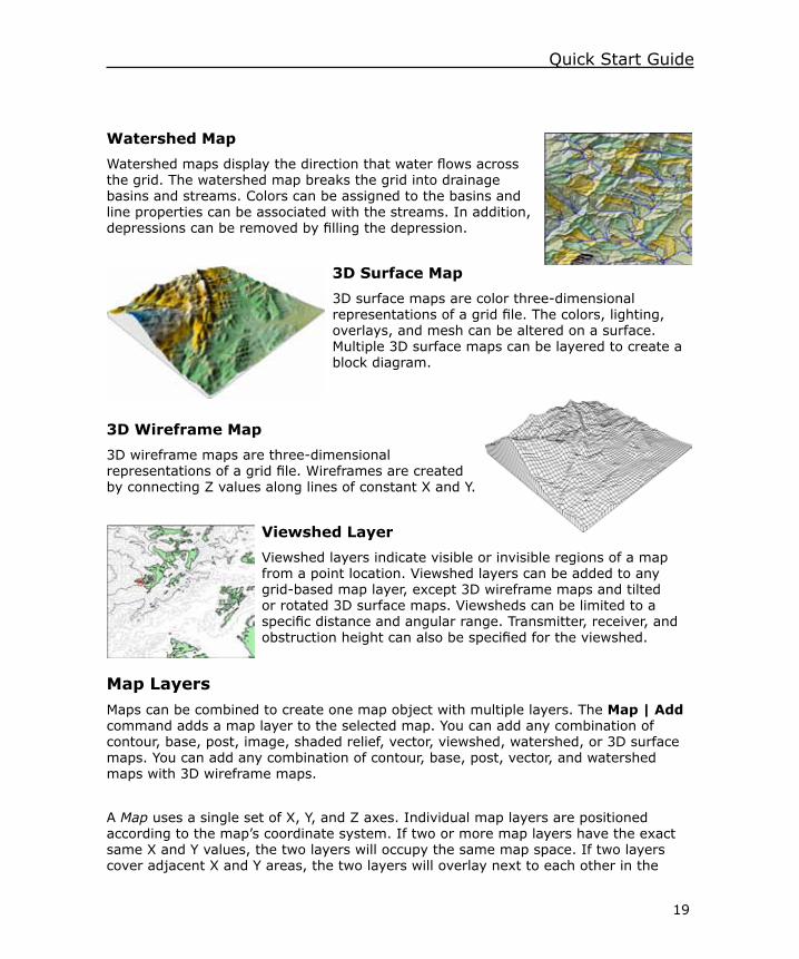
Watershed MapWatershed maps display the direction that water flows across the grid. The watershed map breaks the grid into drainage basins and streams. Colors can be assigned to the basins and line properties can be associated with the streams. In addition, depressions can be removed by filling the depression.

3D Surface Map3D surface maps are color three-dimensional representations of a grid file. The colors, lighting, overlays, and mesh can be altered on a surface. Multiple 3D surface maps can be layered to create a block diagram.

3D Wireframe Map3D wireframe maps are three-dimensional representations of a grid file. Wireframes are created by connecting Z values along lines of constant X and Y.

Viewshed LayerViewshed layers indicate visible or invisible regions of a map from a point location. Viewshed layers can be added to any grid-based map layer, except 3D wireframe maps and tilted or rotated 3D surface maps. Viewsheds can be limited to a specific distance and angular range. Transmitter, receiver, and obstruction height can also be specified for the viewshed.

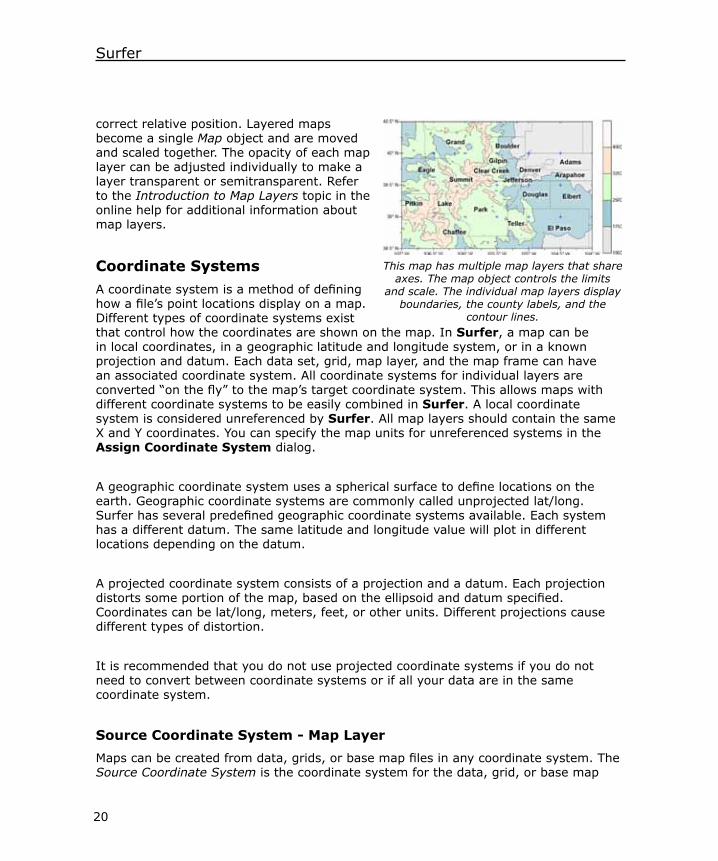
Map LayersMaps can be combined to create one map object with multiple layers. The Map | Add command adds a map layer to the selected map. You can add any combination of contour, base, post, image, shaded relief, vector, viewshed, watershed, or 3D surface maps. You can add any combination of contour, base, post, vector, and watershed maps with 3D wireframe maps.

A Map uses a single set of X, Y, and Z axes. Individual map layers are positioned according to the map’s coordinate system. If two or more map layers have the exact same X and Y values, the two layers will occupy the same map space. If two layers cover adjacent X and Y areas, the two layers will overlay next to each other in the

20

Surfer

correct relative position. Layered maps become a single Map object and are moved and scaled together. The opacity of each map layer can be adjusted individually to make a layer transparent or semitransparent. Refer to the Introduction to Map Layers topic in the online help for additional information about map layers.

Coordinate SystemsA coordinate system is a method of defining how a file’s point locations display on a map. Different types of coordinate systems exist that control how the coordinates are shown on the map. In Surfer, a map can be in local coordinates, in a geographic latitude and longitude system, or in a known projection and datum. Each data set, grid, map layer, and the map frame can have an associated coordinate system. All coordinate systems for individual layers are converted “on the fly” to the map’s target coordinate system. This allows maps with different coordinate systems to be easily combined in Surfer. A local coordinate system is considered unreferenced by Surfer. All map layers should contain the same X and Y coordinates. You can specify the map units for unreferenced systems in the Assign Coordinate System dialog.

A geographic coordinate system uses a spherical surface to define locations on the earth. Geographic coordinate systems are commonly called unprojected lat/long. Surfer has several predefined geographic coordinate systems available. Each system has a different datum. The same latitude and longitude value will plot in different locations depending on the datum.

A projected coordinate system consists of a projection and a datum. Each projection distorts some portion of the map, based on the ellipsoid and datum specified. Coordinates can be lat/long, meters, feet, or other units. Different projections cause different types of distortion.

It is recommended that you do not use projected coordinate systems if you do not need to convert between coordinate systems or if all your data are in the same coordinate system.

Source Coordinate System - Map LayerMaps can be created from data, grids, or base map files in any coordinate system. The Source Coordinate System is the coordinate system for the data, grid, or base map

This map has multiple map layers that share axes. The map object controls the limits

and scale. The individual map layers display boundaries, the county labels, and the

contour lines.

21

Quick Start Guide

file used to create the map layer. Each map layer can reference a different projection and datum. When a map layer has a source coordinate system different than what you want the map to display, the map is converted to the map’s Target Coordinate System.

3D surface maps and wireframe maps do not have an associated coordinate system. When a map with a coordinate system is overlaid onto either of these map types, the map coordinate system is removed and the maps are displayed in the Cartesian coordinates.

Target Coordinate System - MapMaps can be displayed in any coordinate system. The map is displayed in the coordinate system defined as the Target Coordinate System. A coordinate system normally has a defined projection and datum. When a map layer uses a different Source Coordinate System than the map’s Target Coordinate System, the map layer is converted to the map’s Target Coordinate System.

Using Coordinate Systems with Multiple Map LayersThe standard procedure for creating maps in a specific coordinate system are,1. Create the map by clicking on the appropriate Map | New command.2. Click on the map layer to select it. In the Property Manager, click on the

Coordinate System tab.3. If the Coordinate system is not correct, click the Set button next to Coordinate

system. The Assign Coordinate System dialog opens.4. Make any changes in the dialog. This is the initial coordinate system for the map

layer. When finished making changes, click OK.5. To change the coordinate system in which the map is displayed, click on the Map

object in the Object Manager. 6. In the Property Manager, click on the Coordinate System tab.7. If the Coordinate system is not the desired output system, click the Change button

to set the desired target coordinate system. When finished, click OK.8. All of the map layers are converted on the fly to the target coordinate system. The

entire map is now displayed in the desired target system.

Surfer does not require a map projection be defined. Maps can be created from unreferenced data, grid, and map layers. As long as all map layers have the same X and Y ranges, coordinate systems do not need to be specified. If you do not specify a source coordinate system for each map layer, it is highly recommended that you do not change the target coordinate system. Changes to the target coordinate system for the map can cause the unreferenced map layers to appear incorrectly or to not appear.

22

Surfer

TutorialThe tutorial is designed to introduce basic Surfer features and should take less than an hour to complete. After you have completed the tutorial, you will have the skills needed to create maps in Surfer using your own data. The tutorial can be accessed in the program using the Help | Tutorial command.

Tutorial Lesson OverviewThe following is an overview of lessons included in the tutorial:• Lesson 1 - Viewing and Creating Data opens and edits an existing data file and

creates a new data file.• Lesson 2 - Creating a Grid File creates a grid file, the basis for most map types in

Surfer.• Lesson 3 - Creating a Contour Map creates and edits a contour map.• Lesson 4 - Modifying an Axis edits the axis tick labels and axis title.• Lesson 5 - Posting Data Points and Working with Map Layers adds a post map

layer, displaying data points on the contour map. Both maps share the same axes, limits, and scaling.

• Lesson 6 - Creating a Profile shows how to create a profile line on the contour map and automatically display the profile.

• Lesson 7 - Saving a Map shows how to save the Surfer project.• Lesson 8 - Creating a 3D Surface Map creates and edits a 3D surface map.• Lesson 9 - Adding Transparency, Color Scales, and Titles changes the transparency

of objects, adds a color scale, and adds a map title.• Lesson 10 - Creating Maps from Different Coordinate Systems loads multiple map

layers from different coordinate systems and changes the final target coordinate system.

The lessons should be completed in order; however, they do not need to be completed at the same time. Advanced lessons are available in Surfer by clicking Help | Tutorial. The advanced lessons are optional, but we encourage you to read through them to provide additional detailed knowledge about Surfer’s features.

Using the Tutorial with the Demo VersionSome Surfer features are disabled in the demo version, which means that some steps, such as Lesson 7, cannot be completed by users running the demo version. This is noted in the tutorial lessons.

23

Quick Start Guide

Starting SurferTo begin a Surfer session,1. Navigate to the installation folder, which is C:\Program Files\Golden Software\

Surfer 13, by default.2. Double-click on the Surfer.exe application file.3. The Welcome dialog appears. Click New Plot to open a new blank plot window.4. A new empty plot window opens in Surfer. This is the work area where you can

produce grid files, maps, and modify grids.

If this is the first time that you have opened Surfer, you will be prompted for your serial number. Your serial number is located on the CD cover, or in the email download instructions, depending on how you purchased Surfer.

Lesson 1 - Viewing and Creating DataAn XYZ data file is a file containing at least three columns of data values. The first two columns are the X and Y coordinates for the data points. The third column is the Z value assigned to the XY point. Frequently, the X, Y, and Z data are stored in columns A, B, and C, respectively, though this is not required. Data files can contain header information, labels, point identifiers, filter information, and multiple columns of additional data.

Opening an Existing Data File

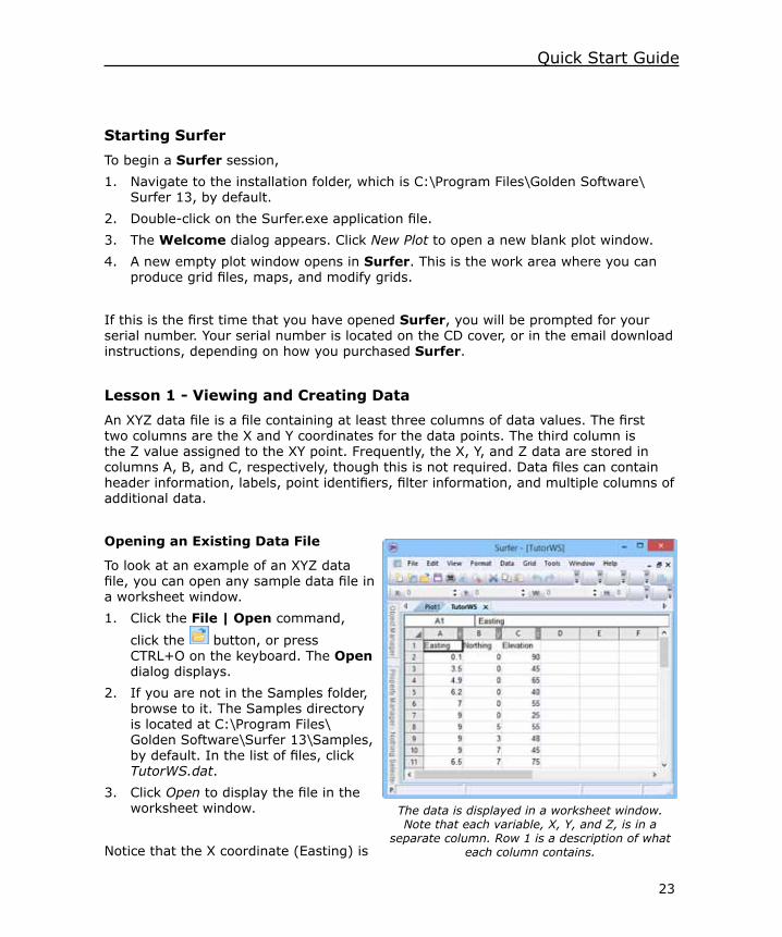
To look at an example of an XYZ data file, you can open any sample data file in a worksheet window.1. Click the File | Open command,

click the button, or press CTRL+O on the keyboard. The Open dialog displays.

2. If you are not in the Samples folder, browse to it. The Samples directory is located at C:\Program Files\Golden Software\Surfer 13\Samples, by default. In the list of files, click TutorWS.dat.

3. Click Open to display the file in the worksheet window.

Notice that the X coordinate (Easting) is

The data is displayed in a worksheet window. Note that each variable, X, Y, and Z, is in a

separate column. Row 1 is a description of what each column contains.

24

Surfer

in column A, the Y coordinate (Northing) is in column B, and the Z value (Elevation) is in column C. Although it is not required, row 1 contains header text, which is helpful in identifying which column contains which data. When a header row exists, the information in the header row is used in the Property Manager when selecting worksheet columns.

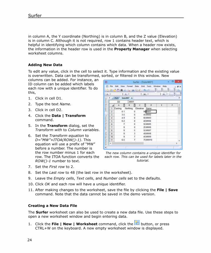
Adding New Data

To edit any value, click in the cell to select it. Type information and the existing value is overwritten. Data can be transformed, sorted, or filtered in this window. New columns can be added. For instance, an ID column can be added which labels each row with a unique identifier. To do this,1. Click in cell D1.2. Type the text Name.3. Click in cell D2.4. Click the Data | Transform

command.5. In the Transform dialog, set the

Transform with to Column variables.6. Set the Transform equation to

D=“MW”+ITOA(ROW()-1). This equation will use a prefix of “MW” before a number. The number is the row number minus 1 for each row. The ITOA function converts the ROW()-1 number to text.

7. Set the First row to 2.8. Set the Last row to 48 (the last row in the worksheet).9. Leave the Empty cells, Text cells, and Number cells set to the defaults.10. Click OK and each row will have a unique identifier.11. After making changes to the worksheet, save the file by clicking the File | Save

command. Note that the data cannot be saved in the demo version.

Creating a New Data File

The Surfer worksheet can also be used to create a new data file. Use these steps to open a new worksheet window and begin entering data.

1. Click the File | New | Worksheet command, click the button, or press CTRL+W on the keyboard. A new empty worksheet window is displayed.

The new column contains a unique identifier for each row. This can be used for labels later in the

tutorial.

25

Quick Start Guide

2. Data are entered into the active cell of the worksheet. The active cell is selected by clicking on the cell or by using the arrow keys to move between cells. When a cell is active, enter a value or text, and the information is displayed in both the active cell and the active cell edit box.

3. To preserve the typed data in the active cell, move to a new cell by clicking a new cell with the mouse, pressing one of the arrow keys, or pressing ENTER. Press the ESC key to cancel without entering the data.

Refer to the Worksheet Window section on page 12 of this guide for additional information about the various parts of the worksheet window.

Saving the Data File

When all of the data has been entered, the data can be saved in a variety of formats. Note that the data cannot be saved in the demo version.

1. Click the File | Save command, click the button, or press CTRL+S on the keyboard. The Save As dialog is displayed if the data was not previously saved.

2. In the Save as type list, choose the DAT Data (*.dat) option.3. Type the name of the file into the File name box.4. Click the Save button and the Data Export Options dialog opens.5. Accept the defaults in the Data Export Options dialog and click OK.6. The file is saved in the Data .DAT format with the file name you specified. The

name of the data file appears in the title bar and on the worksheet tab.

Lesson 2 - Creating a Grid FileGrid files are required to produce a grid-based map. Grid-based maps include contour, image, shaded relief, vector, viewshed, watershed, 3D wireframe, and 3D surface map layers. Grid files are created using the Grid | Data command. The Grid | Data command requires data in three columns: one column containing X data, one column containing Y data, and one column containing Z data. We will use the TutorWS.dat sample file with this lesson.1. In the plot or worksheet window, click the Grid | Data command.2. In the Open Data dialog, click the TutorWS.dat Samples file in the Open

worksheets section of the dialog by clicking once on the file name. The name appears in the File name box below the list of data files.

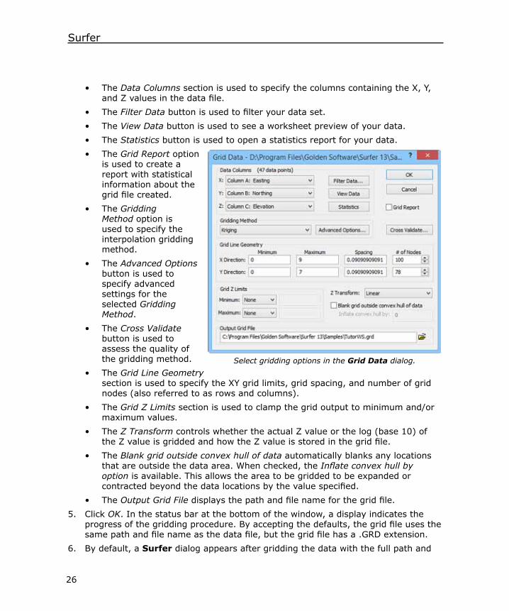
3. Click Open.4. The Grid Data dialog is displayed, where the gridding parameters and preferences

are controlled. Take a moment to look over the various options in the dialog. Do not make any changes at this time, as the default parameters create an acceptable grid file.

26

Surfer

• The Data Columns section is used to specify the columns containing the X, Y, and Z values in the data file.

• The Filter Data button is used to filter your data set.• The View Data button is used to see a worksheet preview of your data.• The Statistics button is used to open a statistics report for your data.• The Grid Report option

is used to create a report with statistical information about the grid file created.

• The Gridding Method option is used to specify the interpolation gridding method.

• The Advanced Options button is used to specify advanced settings for the selected Gridding Method.

• The Cross Validate button is used to assess the quality of the gridding method.

• The Grid Line Geometry section is used to specify the XY grid limits, grid spacing, and number of grid nodes (also referred to as rows and columns).

• The Grid Z Limits section is used to clamp the grid output to minimum and/or maximum values.

• The Z Transform controls whether the actual Z value or the log (base 10) of the Z value is gridded and how the Z value is stored in the grid file.

• The Blank grid outside convex hull of data automatically blanks any locations that are outside the data area. When checked, the Inflate convex hull by option is available. This allows the area to be gridded to be expanded or contracted beyond the data locations by the value specified.

• The Output Grid File displays the path and file name for the grid file.5. Click OK. In the status bar at the bottom of the window, a display indicates the

progress of the gridding procedure. By accepting the defaults, the grid file uses the same path and file name as the data file, but the grid file has a .GRD extension.

6. By default, a Surfer dialog appears after gridding the data with the full path and

Select gridding options in the Grid Data dialog.

27

Quick Start Guide

file name of the grid file that was created. Click OK to close the dialog.7. If Grid Report was checked, a detailed gridding report is displayed. You can

minimize or close this report.

Lesson 3 - Creating a Contour MapA contour map is a plot of three values. The first two dimensions are the X and Y coordinates. Changing the X and Y coordinates changes the size or limits of the map. The third dimension is the Z value, represented by lines of equal value on the map. The shape of the surface is shown by the contour lines.

Contour maps are used for a variety of applications. You can contour any Z value of data. If you have multiple Z values for your X, Y values, you can create multiple contour maps. For example, you could create a contour map for X, Y, Z (elevation) to show the topography of your study area. You could then create a contour map for X, Y, Z (concentration) to show the concentration values across your study area. The Z value could be temperature, concentration, frequency, or any other numeric column of data.

The Map | New | Contour Map command creates a contour map based on a grid file. This lesson will create a contour map from the .GRD file created in Lesson 2 - Creating a Grid File.1. If you have the worksheet window open, click the Window | Plot1 command,

or click on the Plot1 tab. Alternatively, you can create a new plot window with the File | New | Plot command.

2. Click the Map | New | Contour Map command or

click the button.3. The Open Grid dialog

is displayed. Select the TutorWS.grd file created in Lesson 2 - Creating a Grid File by clicking once on its name. The file name is entered in the File name box.

4. Click Open and the map is created using the default contour map properties.5. If you want the contour map to fill the window, click the View | Fit to Window

command, click the button, or press CTRL+D on the keyboard. Alternatively, if you have a wheel mouse, roll the wheel forward to zoom in on the contour map. Click and hold the wheel button straight down while you move the mouse to pan around the screen.

Click on the Plot1 tab to view Plot1 in the plot window.

28

Surfer

Changing Contour Levels

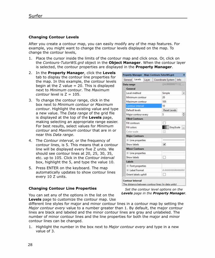
After you create a contour map, you can easily modify any of the map features. For example, you might want to change the contour levels displayed on the map. To change the contour levels,1. Place the cursor inside the limits of the contour map and click once. Or, click on

the Contours-TutorWS.grd object in the Object Manager. When the contour layer is selected, the contour properties are displayed in the Property Manager.

2. In the Property Manager, click the Levels tab to display the contour line properties for the map. In this example, the contour levels begin at the Z value = 20. This is displayed next to Minimum contour. The Maximum contour level is Z = 105.

3. To change the contour range, click in the box next to Minimum contour or Maximum contour. Highlight the existing value and type a new value. The Data range of the grid file is displayed at the top of the Levels page, making selecting an appropriate range easier. For best results, select values for Minimum contour and Maximum contour that are in or near this Data range.

4. The Contour interval, or the frequency of contour lines, is 5. This means that a contour line will be displayed every five Z units. We should see contour lines at 20, 25, 30, 35, etc. up to 105. Click in the Contour interval box, highlight the 5, and type the value 10.

5. Press ENTER on the keyboard. The map automatically updates to show contour lines every 10 Z units.

Changing Contour Line Properties

You can set any of the options in the list on the Levels page to customize the contour map. Use different line styles for major and minor contour lines in a contour map by setting the Major contour every value to a number greater than 1. By default, the major contour lines are black and labeled and the minor contour lines are gray and unlabeled. The number of minor contour lines and the line properties for both the major and minor contour lines can be changed.1. Highlight the number in the box next to Major contour every and type in a new

value of 3.

Set the contour level options on the Levels page in the Property Manager.

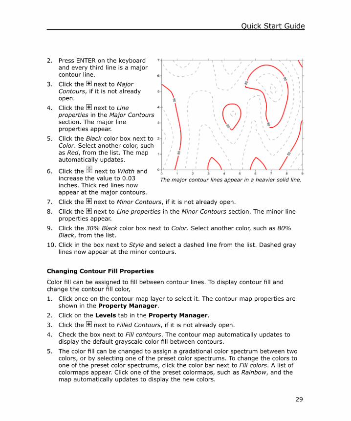
29

Quick Start Guide

2. Press ENTER on the keyboard and every third line is a major contour line.

3. Click the next to Major Contours, if it is not already open.

4. Click the next to Line properties in the Major Contours section. The major line properties appear.

5. Click the Black color box next to Color. Select another color, such as Red, from the list. The map automatically updates.

6. Click the next to Width and increase the value to 0.03 inches. Thick red lines now appear at the major contours.

7. Click the next to Minor Contours, if it is not already open.8. Click the next to Line properties in the Minor Contours section. The minor line

properties appear.9. Click the 30% Black color box next to Color. Select another color, such as 80%

Black, from the list.10. Click in the box next to Style and select a dashed line from the list. Dashed gray

lines now appear at the minor contours.

Changing Contour Fill Properties

Color fill can be assigned to fill between contour lines. To display contour fill and change the contour fill color,1. Click once on the contour map layer to select it. The contour map properties are

shown in the Property Manager.2. Click on the Levels tab in the Property Manager.3. Click the next to Filled Contours, if it is not already open.4. Check the box next to Fill contours. The contour map automatically updates to

display the default grayscale color fill between contours.5. The color fill can be changed to assign a gradational color spectrum between two

colors, or by selecting one of the preset color spectrums. To change the colors to one of the preset color spectrums, click the color bar next to Fill colors. A list of colormaps appear. Click one of the preset colormaps, such as Rainbow, and the map automatically updates to display the new colors.

The major contour lines appear in a heavier solid line.

30

Surfer

6. If only a minimum and maximum color are desired, click the button next to the colormap beside Fill colors. The Colormap dialog appears.

7. The Colormap dialog allows you to select colors to assign to specific Z values. Click the colormap next to Presets. Select GrayScale from the list.

8. Click on the left node below the color spectrum. This selects the minimum color node.

9. Click on the color button next to Color and select the color Blue in the color list. The color scale now ranges from Blue to White. Alternatively, you could select an existing color spectrum from the Presets list, or a custom colormap by clicking the Load button.

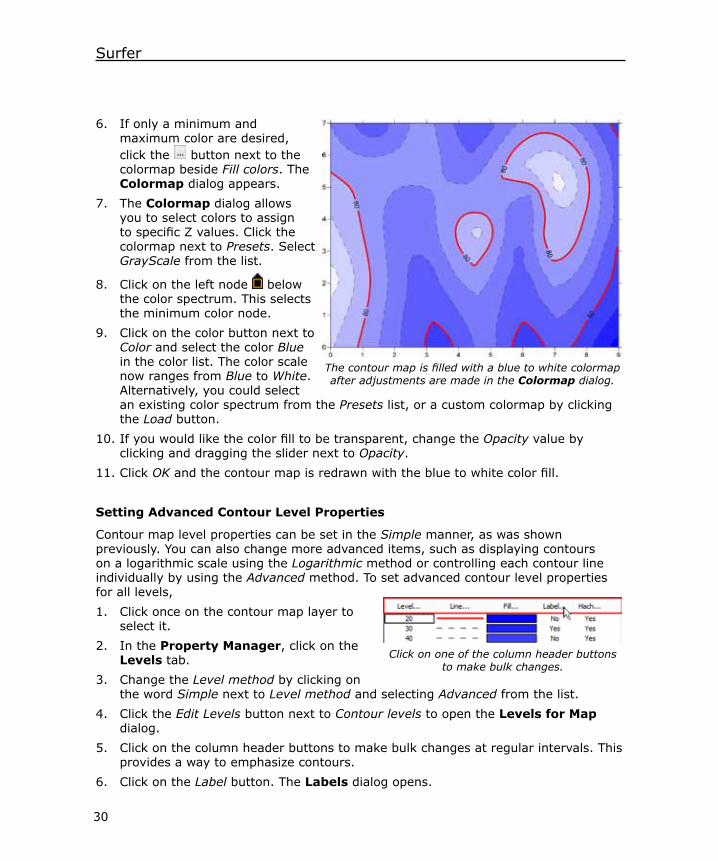
10. If you would like the color fill to be transparent, change the Opacity value by clicking and dragging the slider next to Opacity.

11. Click OK and the contour map is redrawn with the blue to white color fill.

Setting Advanced Contour Level Properties

Contour map level properties can be set in the Simple manner, as was shown previously. You can also change more advanced items, such as displaying contours on a logarithmic scale using the Logarithmic method or controlling each contour line individually by using the Advanced method. To set advanced contour level properties for all levels,1. Click once on the contour map layer to

select it.2. In the Property Manager, click on the

Levels tab.3. Change the Level method by clicking on

the word Simple next to Level method and selecting Advanced from the list.4. Click the Edit Levels button next to Contour levels to open the Levels for Map

dialog.5. Click on the column header buttons to make bulk changes at regular intervals. This

provides a way to emphasize contours.6. Click on the Label button. The Labels dialog opens.

The contour map is filled with a blue to white colormap after adjustments are made in the Colormap dialog.

Click on one of the column header buttons to make bulk changes.

31

Quick Start Guide

7. Change the First value to 2, the Set value to 1, and the Skip value to 2.• The First value tells Surfer which contour line to first change. This will set the

label for the second contour line (Z=30).• The Set value tells Surfer how many contour lines to set with this style. This

says to set one line with the label format.• The Skip value tells Surfer how many lines to skip before setting the next

contour line. This says to skip the next two contour lines. So, the Z=40 and Z=50 contours are not set.

• The next contour line Z = 60 uses the label format. Z=70 and Z=80 are skipped. Z=90 is set. Z=100 is skipped.

8. Click the Font button. The Font Properties dialog opens.9. Set the Size (points) to 12.10. Set the Foreground color and opacity color to White.11. Click OK.12. Click OK in the Labels dialog. Notice how the label status is changed in the Levels

for Map dialog.13. Click on the Hach button. The Hachures dialog opens.14. Set the First to 1, the Set to 1, and the Skip to 0. This will set all contour lines to

show the hachure setting.15. Check the Hachure Closed Contours Only box, if it is not already checked.16. Change the Direction to Uphill.17. Click OK. This changes all of the items under Hach to Yes. All closed contours will

have hachure marks.18. Click OK and the bulk changes are made to the contour map.

To set advanced contour level properties for individual levels,1. Click once on the contour map layer to select it.2. In the Property Manager, click

on the Levels tab.3. Make sure that the Level method is

set to Advanced.4. Click the Edit Levels button next to

Contour levels to open the Levels for Map dialog.

5. In the Levels for Map dialog, you can double-click an individual Z value in the list underneath the Level button to change the Z value for that particular contour level. Double-click on the number 60.

6. In the Z Level dialog, highlight the value 60 and type 65.

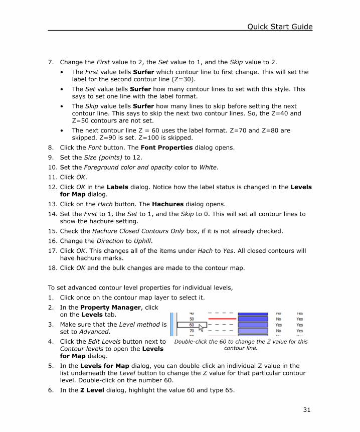
Double-click the 60 to change the Z value for this contour line.

32

Surfer

7. Click OK and the contour line changes to 65.8. You can also double-click the line style for an individual level to modify the line

properties for the selected level. This provides a way to emphasize individual contour levels on the map. Double-click on the line style next to the 70.

9. In the Line Properties dialog, change the Style to a solid line by clicking on the existing dashed line and selecting the Solid line from the list.

10. Click OK.11. Let’s add a single contour line halfway between two existing values. Click on the

number 65 under the Level column.12. Click the Add button. The value 57.5 is added between the 50 and the 65.13. Click OK and the individual settings are made to the contour map.

Adding, Deleting, and Moving Contour Labels

Contour label locations can be changed on an individual basis. Labels can be added, deleted, or moved. To add, delete, and move contour labels,1. Click once on the contour map layer to select it.2. Click the Map | Edit Contour Labels command or right-click on the contour map

layer and select Edit Contour Labels. The cursor changes to to indicate that you are in edit mode. Contour labels have rectangular boxes around them in edit mode.

3. To delete a label, click on the label and press the DELETE key on the keyboard. For example, left-click on one of the center 65 labels and press the DELETE key on your keyboard.

4. To add a label, press and hold the CTRL key on the keyboard. The cursor changes

to to indicate you are able to add a new label. Left-click the location on the contour line where you want the new label to be located. Add several contour labels by clicking on the contour lines.

5. To move a contour label, left-click on the label, hold down the left mouse button, and drag the label. Release the left mouse button to complete the label movement.

6. To duplicate a label, hold the CTRL key on the keyboard while clicking and dragging with the left mouse button on an existing label. Drag the duplicate label to a new location along the line.

7. To exit the Edit Contour Labels mode, press the ESC key.

Lesson 4 - Modifying an AxisEvery contour map is created with four map axes: the bottom, right, top, and left axes. 3D maps have an additional Z axis. Additional X, Y, or Z axes can be added to a map with the Map | Add command. You can control the display of each axis

33

Quick Start Guide

independently of the other axes on the map. In this example, we will change the axis label spacing and add an axis title.

Adding an Axis Title

To add an axis title to an axis,1. Move the cursor over one of the axis tick labels on the bottom X axis and left-click

the mouse. In the status bar at the bottom of the plot window, the words “Map: Bottom Axis” are displayed. The Bottom Axis object is selected in the Object Manager. This indicates that you have selected the bottom axis of the map. Additionally, blue circle handles appear at each end of the axis, and green square handles appear surrounding the entire map. This indicates that the axis is a “sub-object” of the entire map.

2. The bottom axis properties are displayed in the Property Manager. Click on the General tab.

3. Click the next to Title to open the Title section, if it is not already open.4. Click in the box next to Title text. Type Bottom Axis and press the ENTER key on

the keyboard. This places a title on the selected axis. Alternatively, click the button. Type the text in the Text Editor and click OK.

5. If you cannot see the axis title, click the View | Zoom | Selected command. The map automatically increases its size to fill the plot window.

Changing the Tick Label Properties

All properties of the axis are editable, including the tick label format and frequency. To change the axis tick labels,1. In the Property Manager, click on the Scaling tab to display the axis scaling

options.2. In the Major interval box, highlight the value 1 and type the value 1.5.3. Press ENTER on the keyboard and the spacing automatically updates on the map

axis to show 1.5 units between tick marks.4. Click on the General tab in the Property Manager. 5. Click the next to Labels, if it is not already open.6. Click the next to Label Format to open the Label Format section.7. In the Label Format

section, click on the existing option for Type and select Fixed from the list.

8. Highlight the existing value next to Decimal

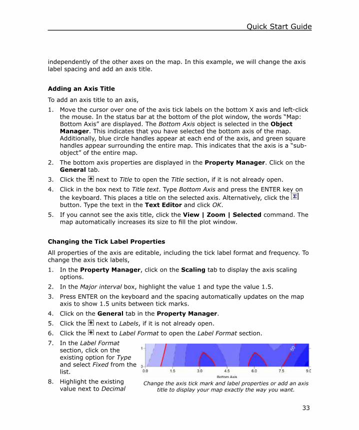
Change the axis tick mark and label properties or add an axis title to display your map exactly the way you want.

34

Surfer

digits and type the value 1.9. Press ENTER on the keyboard. This indicates that only one digit follows the decimal

point for the axis tick labels.10. The map is updated immediately after every change, showing the axis tick

spacing, labels, and the axis title.

Lesson 5 - Posting Data Points and Working with LayersPost maps are created by placing symbols representing data points at the X, Y data point locations on a map. Posting data points on a map can be useful in determining the distribution of data points, as well as placing data or text information at specific points on the map. Data files contain the X, Y coordinates used to position the points on the map. Data files can also contain the labels associated with each point.

Multiple map layers can be added to an existing map to display a variety of map types. The map uses a single set of axes and the map layers are positioned according to the target coordinate system. For example, you can add a post map layer with the location and station names of each data collection station to a contour map of weather data.

When a new post map is created with Map | New | Post Map it is independent of any other maps in the current plot window. When the two maps are displayed, two sets of axes are also displayed, one set for each map. When you select a map and click the Map | Add command, a new map layer can be added to the selected map.

If two maps already existed, a map layer can be dragged to a different map object in the Object Manager. Alternatively, select both maps and click the Map | Overlay Maps command. All selected map layers are moved to a single map object.

Adding a Post Map Layer

If you have not already completed Lesson 1 - Viewing and Creating Data, do so now. This lesson adds a worksheet column that is used for the post map labels.1. Click once on Contours-TutorWS.grd layer in the Object Manager to select it.2. Click the Map | Add | Post Layer command, or right-click on the contour map

and select Add | Post Layer.3. In the Open Data dialog, select TutorWS.dat from the Open worksheets section.

If the TutorWS.dat file is not already open, select it from the Samples folder.4. Click Open.

Notice in the Object Manager that the post map layer has been added to the Map. The two map layers now share the same set of axes. Changes made to the map

35

Quick Start Guide

properties will affect both the contour map layer and the post map layer.

Editing the Post Map

Once you have created a post map layer, you can customize the post map properties. Symbols in a post map can all be the same or can be selected with a worksheet column. Symbol sizes can all be the same or have proportional sizes. Symbol colors can all be the same or have color based on a column. To change the post map properties,1. Click on the Post-TutorWS.dat layer in the Object

Manager or in the plot window.2. In the Property Manager, click on the Symbol

tab.3. Click the next to Symbol, if it is not already

open.4. Click the next to Symbol properties to open the Symbol properties section.5. Next to the Symbol, click on the existing symbol. Click on the filled diamond

symbol (Symbol set: GSI Default Symbols, Number: 6) in the list.6. Next to Fill color, click on the existing color. In the list, select the Cyan color. The

symbol is now cyan with a black outline.7. Fill opacity and Line opacity can be adjusted to create semi-transparent symbols

by dragging the next to Fill opacity or Line opacity, if desired.8. Click the next to Symbol Size, if necessary.9. Highlight the value next to the Symbol size option and type 0.09 in.10. Press ENTER on the keyboard. The symbols update with the new symbol size.11. Click the next to Symbol Color, if necessary.12. To change the symbol colors based on a worksheet value, click on the None next

to the Color column option and select Column C: Elevation.13. Verify that the Color method is set to Numeric via colormap.14. Click the colormap next to the Symbol colors and select the desired colormap,

such as Terrain.

If the post map is not visible, ensure that the post layer is on top of the contour layer in the Object Manager. The order the layers are listed in a map object is the order the map layers are drawn in the plot window. To move a map layer, left-click and drag up or down in the map object. Alternatively, select the map layer and use the Arrange | Order Objects command or right-click and select Order Objects.

The post map Symbol page of the Property Manager.

36

Surfer

Adding Labels to the Post Map

You can add labels to the data points on post maps and classed post maps. Multiple labels can be added to display all of the information desired in the map. To add labels,1. Click on the Post-TutorWS.dat layer in the Object Manager to select it.2. In the Property Manager, click on the Labels tab.3. Click the next to Label Set 1, if the section is not already open.4. Next to Worksheet column, click

the word None and select Column C: Elevation from the list.

5. For the Position relative to symbol option, click on the existing option and select Below from the list.

6. Click the Add button next to the Add label set option to add a second label to the post map.

7. Next to Worksheet column, click the word None and select Column D: Name from the list.

8. For the Position relative to symbol option, click on the existing option and select Above from the list.

9. Click the next to Font properties to open the Font properties section.

10. Change the Background opacity to 33%. This places a semi-transparent white box around the names.

Moving Individual Post Map Labels

You can move individual labels of post maps and classed post maps with the Map | Edit Post Labels command. A customizable leader line is automatically added from the data point label to the symbol. To move individual labels,1. Select the Post-TutorWS.dat layer in the Object Manager.2. Click the Map | Edit Post Labels command or right-click on the selected map and

select Edit Post Labels. The cursor will change to to indicate you are now in post label editing mode.

3. Left-click on a label, hold the left mouse button down, and drag the label to a new location. With the left mouse button held down, the arrow keyboard keys can be used to nudge the label location. Release the left mouse button to place the label in the new location. A leader line will be added from the point location to the new

Customize the post map by adding multiple labels with different properties

37

Quick Start Guide

label location by default. The leader line visibility and line properties are controlled on the Labels page in the Property Manager when the post layer is selected.

4. Press the ESC key to exit the post label editing mode.

Lesson 6 - Creating a ProfileThe ability to slice a grid file in Surfer to create a file of data points along a specified line of section is a very powerful tool. The sliced data can be visually displayed as a profile in Surfer, or multiple profiles can be combined to display a cross section. Sometimes, a simpler process is desired because the data is not the end result. If being able to visually see the profile on the map and on a graph is the desire, the Map | Add | Profile command provides an excellent quick method. To start off, you must first have a grid file of your surface data. The profile line will be drawn directly on the map. To create the profile,1. Click once on the contour map layer to select it.

2. Click the Map | Add | Profile command. The cursor changes to to indicate that you are in the drawing mode.

3. Click inside the contour map near the (0,4) and (9,4) coordinate locations. The exact coordinates of the cursor are displayed in the status bar for reference.

4. After the second point has been clicked, a line connects the points. Press ENTER on the keyboard to end drawing mode.

5. Click the View | Fit to Window command to see the entire map and profile.

The base map layer is automatically added to the Map object and the profile graph is automatically created. The properties can be edited by clicking on the Profile 1 object in the Object Manager.

Lesson 7 - Saving a MapWhen you have completed the map in the plot window, you can save the map to a Surfer .SRF file. Surfer .SRF files contain all the information necessary to reproduce the project. When you save a map as a .SRF file, all the scaling, formatting, and map properties are preserved in the file. An asterisk (*) next to the file name in the title bar and plot window tab indicates the file has been modified and the modifications have not yet been saved.

The profile graph showing the elevation change across the drawn line is automatically created when

the line is completed.

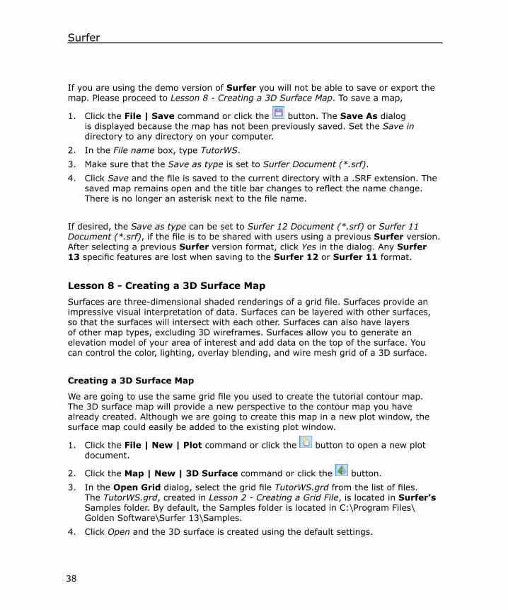
38

Surfer

If you are using the demo version of Surfer you will not be able to save or export the map. Please proceed to Lesson 8 - Creating a 3D Surface Map. To save a map,

1. Click the File | Save command or click the button. The Save As dialog is displayed because the map has not been previously saved. Set the Save in directory to any directory on your computer.

2. In the File name box, type TutorWS.3. Make sure that the Save as type is set to Surfer Document (*.srf).4. Click Save and the file is saved to the current directory with a .SRF extension. The

saved map remains open and the title bar changes to reflect the name change. There is no longer an asterisk next to the file name.

If desired, the Save as type can be set to Surfer 12 Document (*.srf) or Surfer 11 Document (*.srf), if the file is to be shared with users using a previous Surfer version. After selecting a previous Surfer version format, click Yes in the dialog. Any Surfer 13 specific features are lost when saving to the Surfer 12 or Surfer 11 format.

Lesson 8 - Creating a 3D Surface MapSurfaces are three-dimensional shaded renderings of a grid file. Surfaces provide an impressive visual interpretation of data. Surfaces can be layered with other surfaces, so that the surfaces will intersect with each other. Surfaces can also have layers of other map types, excluding 3D wireframes. Surfaces allow you to generate an elevation model of your area of interest and add data on the top of the surface. You can control the color, lighting, overlay blending, and wire mesh grid of a 3D surface.

Creating a 3D Surface Map

We are going to use the same grid file you used to create the tutorial contour map. The 3D surface map will provide a new perspective to the contour map you have already created. Although we are going to create this map in a new plot window, the surface map could easily be added to the existing plot window.

1. Click the File | New | Plot command or click the button to open a new plot document.

2. Click the Map | New | 3D Surface command or click the button.3. In the Open Grid dialog, select the grid file TutorWS.grd from the list of files.

The TutorWS.grd, created in Lesson 2 - Creating a Grid File, is located in Surfer’s Samples folder. By default, the Samples folder is located in C:\Program Files\ Golden Software\Surfer 13\Samples.

4. Click Open and the 3D surface is created using the default settings.

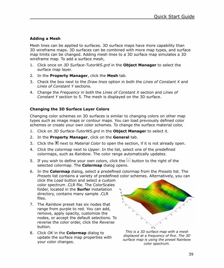
39

Quick Start Guide

Adding a Mesh

Mesh lines can be applied to surfaces. 3D surface maps have more capability than 3D wireframe maps. 3D surfaces can be combined with more map types, and surface map limits can be changed. Adding mesh lines to a 3D surface map simulates a 3D wireframe map. To add a surface mesh,1. Click once on 3D Surface-TutorWS.grd in the Object Manager to select the

surface map layer.2. In the Property Manager, click the Mesh tab.3. Check the box next to the Draw lines option in both the Lines of Constant X and

Lines of Constant Y sections.4. Change the Frequency in both the Lines of Constant X section and Lines of

Constant Y section to 5. The mesh is displayed on the 3D surface.

Changing the 3D Surface Layer Colors

Changing color schemes on 3D surfaces is similar to changing colors on other map types such as image maps or contour maps. You can load previously defined color schemes or create your own color schemes. To change the surface material color,1. Click on 3D Surface-TutorWS.grd in the Object Manager to select it.2. In the Property Manager, click on the General tab.3. Click the next to Material Color to open the section, if it is not already open.4. Click the colormap next to Upper. In the list, select one of the predefined

colormaps, such as Rainbow. The color range automatically updates.

5. If you wish to define your own colors, click the button to the right of the selected colormap. The Colormap dialog opens.

6. In the Colormap dialog, select a predefined colormap from the Presets list. The Presets list contains a variety of predefined color schemes. Alternatively, you can click the Load button and select a custom color spectrum .CLR file. The ColorScales folder, located in the Surfer installation directory, contains many sample .CLR files.

7. The Rainbow preset has six nodes that range from purple to red. You can add, remove, apply opacity, customize the nodes, or accept the default selections. To reverse the color order, click the Reverse button.

8. Click OK in the Colormap dialog to update the surface map properties with your color changes.

This is a 3D surface map with a mesh displayed at a frequency of five. The 3D surface map is using the preset Rainbow

color spectrum.

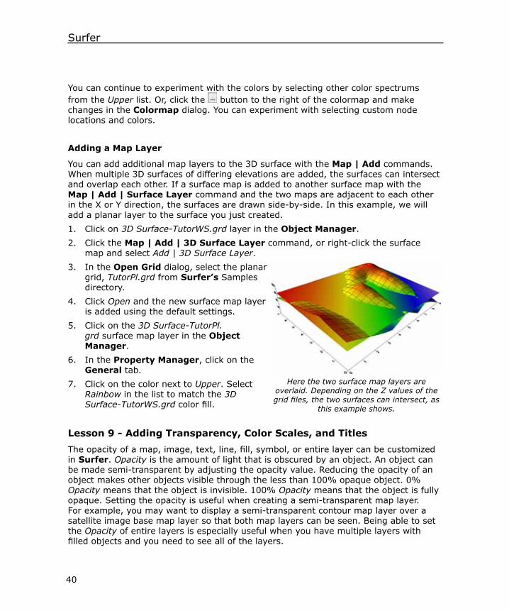
40

Surfer

You can continue to experiment with the colors by selecting other color spectrums from the Upper list. Or, click the button to the right of the colormap and make changes in the Colormap dialog. You can experiment with selecting custom node locations and colors.

Adding a Map Layer

You can add additional map layers to the 3D surface with the Map | Add commands. When multiple 3D surfaces of differing elevations are added, the surfaces can intersect and overlap each other. If a surface map is added to another surface map with the Map | Add | Surface Layer command and the two maps are adjacent to each other in the X or Y direction, the surfaces are drawn side-by-side. In this example, we will add a planar layer to the surface you just created.1. Click on 3D Surface-TutorWS.grd layer in the Object Manager.2. Click the Map | Add | 3D Surface Layer command, or right-click the surface

map and select Add | 3D Surface Layer.3. In the Open Grid dialog, select the planar

grid, TutorPl.grd from Surfer’s Samples directory.

4. Click Open and the new surface map layer is added using the default settings.

5. Click on the 3D Surface-TutorPl.grd surface map layer in the Object Manager.

6. In the Property Manager, click on the General tab.

7. Click on the color next to Upper. Select Rainbow in the list to match the 3D Surface-TutorWS.grd color fill.

Lesson 9 - Adding Transparency, Color Scales, and TitlesThe opacity of a map, image, text, line, fill, symbol, or entire layer can be customized in Surfer. Opacity is the amount of light that is obscured by an object. An object can be made semi-transparent by adjusting the opacity value. Reducing the opacity of an object makes other objects visible through the less than 100% opaque object. 0% Opacity means that the object is invisible. 100% Opacity means that the object is fully opaque. Setting the opacity is useful when creating a semi-transparent map layer. For example, you may want to display a semi-transparent contour map layer over a satellite image base map layer so that both map layers can be seen. Being able to set the Opacity of entire layers is especially useful when you have multiple layers with filled objects and you need to see all of the layers.

Here the two surface map layers are overlaid. Depending on the Z values of the grid files, the two surfaces can intersect, as

this example shows.

41

Quick Start Guide

Creating a Filled Contour Map

To create a contour map,

1. Click the File | New | Plot command or the button to create a new plot window.

2. Click the Map | New | Contour Map command.3. Select the grid file Golden.grd from the list of files in the Open Grid dialog. The

Golden.grd file is located in Surfer’s Samples folder.4. Click Open. The map is created using the default settings. Some settings are

persistent while Surfer is open. If you’ve completed Lesson 3 - Creating a Contour Map in the same session, the map created in this step will have uphill hachures and white-text contour labels.

5. Click on the contour map layer to select it.6. In the Property Manager, click on the Levels tab.7. Set the Level method to Simple, if it is not already Simple.8. Click the next to Filled Contours to open the Filled Contours section, if it is not

already open.9. Check the box next to Fill contours to fill the contours with the default colormap.10. Click the next to Labels to open the Labels section, if it is not already open.11. Click the next to Font properties.12. If the Foreground color is not Black, click the current color and select Black from

the color palette.

Applying Opacity

You can adjust the Opacity value of a map layer, or of individual fill, text, lines, or symbols when the appropriate object is selected. The properties are displayed in the Property Manager. To add transparency to the filled contours,1. Click on the contour map layer to select it.2. Click on the Levels tab in the Property Manager.

3. Click the button next to Fill colors. The Colormap dialog opens.4. Click on the current selection in the Presets list and select Terrain.5. Verify the Apply opacity to ALL nodes check box is checked.6. Highlight the existing 100% value next to the Opacity option and type 30.7. Click OK in the Colormap dialog. The Terrain colormap and 30% opacity setting

is applied to the contour layer’s Fill colors. Notice Custom is displayed in the Fill colors field.

42

Surfer

Adding and Editing a Color Scale Bar

Color scales are legends that show the fill colors. Color scales are available for contour, 3D wireframe, 3D surface, image, and vector maps. The color scale displays the colors assigned to levels in a filled contour map or 3D wireframe, the colors used in an image map or 3D surface, and the fill assigned to vector symbols. To add a color scale and color scale title to the contour map,1. Click on the contour map layer to select it.2. Click on the Levels tab in the Property Manager.3. Click the next to Filled Contours to open the Filled Contours section, if it is not

already open.4. Check the box next to Color scale. A default color scale is created. A new Color

Scale object is added to the Object Manager.5. Click on Color Scale in the Object Manager to select the color scale.6. In the Property Manager, click on the General tab.7. Click the next to Title if the section is not already open.8. To add a title to the color scale bar, click the in the empty box next to Title text. 9. In the Title text field, type Elevation (Feet).10. Press ENTER. The title is added with the default settings.11. Change the title position by clicking the current selection next to Position. Select

Top from the Position list.12. Notice the color scale title moves to the top of the color scale, and the text

orientation automatically changes to horizontal.

Downloading an Online Base Map Layer

A base map layer can be added below the existing semi-transparent contour layer to enhance the map’s appearance. To add a base map layer from an online server,1. With the Map selected, click the Map | Add | Base Layer from Server command

or the button to download an image base map from a web mapping server.

2. In the Download Online Maps dialog, click the next to Imagery.

3. Click the next to the NAIP Color Imagery for US server name.4. Click on the USGS_EROS_Ortho_NAIP layer.5. Notice the Specify Latitude/Longitude extents option is selected with the

boundaries of the selected Map.6. In the Select Image Resolution to Download section, the default setting is

sufficient for this tutorial. Dragging the slider to the right increases the image resolution. The farther to the right the slider is located, the better the resolution and the larger the image. Clicking on one of the lines in the middle toward the

43

Quick Start Guide

left side of the slider downloads a map of sufficient quality that is smaller in size.

7. Click OK and the base layer downloads. The base layer is automatically placed behind the contour layer.

8. Click No if prompted to change the map limits in a Surfer dialog.

Adding a Map Title

Adding a title to a map is a great way to stay organized and create publication quality maps. To add a title to the tutorial map,1. Click on the Top Axis in the Object

Manager to select it.2. In the Property Manager, click on the

General tab.3. Click the next to Title, if the section is

not already open.

4. In the box next to Title text, click the button to open the Text Editor.5. Type Tutorial Map and press the ENTER key on the keyboard.6. On the second line, we will use a dynamic predefined instruction to insert the

current date. Click the button.7. In the Date/Time Format Builder dialog, select the desired date/time format in

the Predefined date/time formats list. For instance, select MM/dd/yy.8. Click Insert. The selected format replaces the previous format in the Date/Time

format (edit to change) box.9. Click OK in the Date/Time Format Builder dialog. Today’s date is added to the

Text Editor.10. Highlight the date in the Text Editor.

11. Click the button to make the highlighted text bold.12. Change the Size (points) to 14. The size is located immediately to the right of the

font name.13. Click OK to close the Text Editor. The map updates to display the map title.

Lesson 10 - Creating Maps from Different Coordinate SystemsMap layers from different coordinate systems can be created in the same map object. Surfer converts the source coordinate system for each map layer to the target coordinate system for the entire map. The axes display the target coordinate system.

The map contains semi-transparent filled contours on a base layer. A color scale and

title were added next to the map.

44

Surfer

Creating the First Map

1. Click the File | New | Plot command or the button to create a new plot.

2. Click the Map | New | Contour Map command or the button to create the first map layer, a new contour map.

3. In the Open Grid dialog, click the Diablo.grd file in the Surfer Samples directory.4. Click Open.5. Click the Contours-Diablo.grd layer in the Object Manager to select the contour

layer.6. In the Property Manager, click on the Coordinate System tab. Note that the

contour layer was imported with a coordinate system already specified. This map layer is in State Plane 1927 - California III (Meters), as shown in the Name field.

Creating a New Map and Assigning a Coordinate System

Maps can be created without predefined coordinate systems and assigned the correct coordinate system in the map properties.

1. Click the Map | New | Post Map command or the button to create a post map. This creates a new map with separate axes.

2. In the Open Data dialog, click the Diablo Example.dat file in the Surfer Samples directory.

3. Click Open.4. Click on the Map that contains the post map. Drag it in the plot window so that the

two maps are side by side. Note that the axes on the two maps have very different coordinates.

5. Click on Post-Diablo Example.dat in the Object Manager to select the post layer.6. In the Property Manager, click on the Coordinate System tab. Note that the

post map does not have a predefined coordinate system.7. Click the Set button to define the coordinate system for the post map. Since we

know this coordinate system, we can set it.8. We can use the search bar to reduce the number of projections listed in the

Assign Coordinate System dialog, since we know the map coordinate system. In the Search for text or EPSG code box, type UTM Zone 10N.

9. Press ENTER or click the button.10. In the Assign Coordinate System dialog, click the next to Predefined to open

the Predefined section.11. Click the next to Projected Systems to open the Projected Systems section.12. Click the next to UTM to open the UTM section.

45

Quick Start Guide

13. Click the next to North America to open the North America section.14. Click on North America NAD27 UTM Zone 10N to select it.15. Click OK. On the Coordinate System page, the post layer shows a defined

coordinate system next to Name.16. In the Object Manager, click and drag the Post-Diablo Example.dat layer into the

Map object that contains the Contours-Diablo.grd layer. The two map layers are now overlaid. You can see the posted symbols are located on the contour lines, despite the different coordinate systems.

Setting the Target Coordinate System

The target coordinate system is the system displayed on the map axes. Once the map layer is defined, the target coordinate system can be changed to any desired coordinate system. To change the target coordinate system,1. Click on the Map object in the Object Manager.2. In the Property Manager, click on the Coordinate System tab.3. Click the Change button.4. In the Assign Coordinate System dialog, click the next to Predefined to open

the Predefined section.5. Click the next to Geographic (lat/lon) to open the Geographic (lat/lon) section.6. Click on World Geodetic System 1984 to select it.7. Click OK. On the Coordinate System page, the map now has a different

coordinate system than either of the map layers. Notice that the axes are now showing latitude and longitude values, as well.

Notice the above section, we did not use the search function in the Assign Coordinate System dialog. We had to scroll to the top of the Coordinate Systems list to locate the Predefined section, and we had to scroll to the bottom of the Geographic (lat/lon) section to select World Geodetic System 1984.

When searching in the Assign Coordinate System dialog, the search string must exactly match a portion of the desired coordinate system name or EPSG code. However, the search string does not need to be the complete name or EPSG code. For example, searching for System 1984 will return the World Geodetic System 1984 coordinate system, but searching for World 1984 returns no results.

Changing the Axis Label Format

The axis labels can be displayed in a variety of number formats. In this section, we will change the axis labels to Degrees, Minutes, Seconds format.

46

Surfer

1. Click on the Left Axis object in the Object Manager.

2. In the Property Manager, click on the General tab to view the General page.

3. Click the next to Labels.4. Click the next to Label Format.5. Click the current option next to Type and

select DMS (Lat/long) from the list.6. Click on the Bottom Axis object in the

Object Manager.7. Repeat steps 2 through 5.8. Click on the Scaling tab in the Property

Manager.9. Highlight the value next to Major interval

and type 0.03.10. The axis labels are now in DMS format.

Printing the Online HelpThe online help topics may be printed. You can print a single topic, a section of the table of contents, or all topics in the table of contents. Open the online help by clicking the Help | Contents command in the Surfer window.

To print one topic, click the topic you wish to print and click the button. If the Contents page is open in the help navigation pane, the Print Topics dialog appears. Select Print the selected topic and click OK.

To print one book, the Tutorial for example, click the Contents tab on the left side of the help window. Click on the book you want to print, such as the Tutorial book, to

select the book. Click the button. In the Print Topics dialog, select Print the selected heading and all subtopics and click OK. All the topics included in the book are printed.

To print all of the topics in the help file table of contents, select the top-level book in

the help book, Surfer 13. Click the button. In the Print Topics dialog, select Print the selected heading and all subtopics and click OK. All the topics included in the online help table of contents are printed.WARNING: Printing the entire help file takes hundreds of letter-sized sheets of paper

The final map displays two overlaid map layers, each in a different source coordinate

system. The map axes display the target coordinate system, and the labels are in

Degrees, Minutes, Seconds format.

47

Quick Start Guide

and is very time consuming to print. There is no table of contents or index printed with the file.

You can purchase the full PDF user’s guide that includes all of the documentation for the program. This PDF user’s guide can be printed by the user, if desired. The guide can be purchased on the Golden Software website at www.GoldenSoftware.com.

Getting HelpThe quick start guide is a quick way to learn the basics in Surfer. There are also other sources of help with Surfer.

Extensive information about Surfer is located in the online help. To access the online help, choose the Help | Contents command. You can navigate help using the Contents, Index, Search, and Favorites pages in the navigation pane to the left of the topic page.

Surfer also contains context-sensitive help. Highlight a menu command, window region, or dialog, press the F1 key, and help is displayed for the highlighted item. You may also access context-sensitive help by pressing SHIFT+F1 or clicking on

the button on the toolbar. Then, click on a menu command, toolbar button, or screen region to view information specific to that item. The help window opens with

information about the selected item. In most dialogs, click the button in the dialog title bar or click the Help button to obtain help for that dialog.

Internet ResourcesThere are several Internet help resources.• Direct links to the Golden Software home page (www.GoldenSoftware.com), the

Surfer product page, frequently asked questions, and the knowledge base are available by clicking Help | Golden Software on the Web.

• The Help | Feedback commands send a problem report, suggestion, or information request by email directly to Surfer technical support.

• Click the Forums button in the online help to post a question or comment to our public support forums.

• Click the Knowledge Base button in the online help to search for an answer in our frequently updated knowledge base.

• Browse newsletter articles on our website at www.GoldenSoftware.com/newsletter.• Browse FAQs at www.GoldenSoftware.com/products/surfer#faqs.

48

Surfer

• Watch training videos and past webinars at www.GoldenSoftware.com/products/surfer#training-videos.

• Read through our blog items at www.GoldenSoftware.com/blog.

Technical SupportGolden Software’s technical support is free to registered users of Golden Software products. Our technical support staff is trained to help you find answers to your questions quickly and accurately. We are happy to answer all of your questions about any of our products, both before and after your purchase. We also welcome suggestions for improvements to our software and encourage you to contact us with any ideas you may have for adding new features and capabilities to our programs.

Technical support is available Monday through Friday 8:00 AM to 5:00 PM Mountain Time, excluding major United States holidays. We respond to email, phone, and fax technical questions within one business day. When contacting us with your question, have the following information available:• Your Surfer serial number (located on the CD shipping cover or in Help | About

Surfer)• Your Surfer version number, found in Help | About Surfer• The operating system you are using (i.e. Windows XP, Vista, 7, 8, or higher)• Whether you are using a 32-bit or 64-bit Surfer program and operating system

If you encounter problems with Surfer, you are welcome to send an email message to Golden Software using the Help | Feedback | Problem Report command. This message is delivered directly to [email protected]. Report the steps you perform when the problem occurs and include the full text of any error messages that are displayed. You are welcome to attach a .ZIP file (10 MB maximum) containing the .SRF file and other files that illustrate the problem or contact technical support if you have very large zipped attachments to send.

Contact InformationTelephone: 303-279-1021Fax: 303-279-0909Email: [email protected]: www.GoldenSoftware.com (includes FAQs, knowledge base, support forum, training videos, newsletters, blogs, downloads, and more!)Mail: Golden Software, LLC; 809 14th Street; Golden, Colorado 80401-1866; USA

49

Quick Start Guide

Index3D surface map 19, 38

3D wireframe map 19

A

active cell 12, 24, 25

arrange objects 10

assign coordinate system 20, 44

automation 1, 5

axis 32, 33, 34

B

base map 14, 17

from server 45

blank grid outside data 15, 26

bold text 4

boundary files 14

breakline 16, 17

C

classed post map 18

colormap 30, 39, 40

commands 4, 7, 8, 9, 14, 47

contact information 48

context-sensitive help 47

contour

fill 29

interval 28

levels 28, 32

map 18, 30, 41

contour map 18

coordinates 9, 13, 15

coordinate system 20, 44, 45

layer 20

map 21

creating a grid file 25

creating a map 5, 27

cross section 37

customize 8

D

data file 13, 23

date formatted axis 4

date/time format 43

demo 22

descending axis 4

docking 8

documentation 3, 46

E

edit labels 32, 36

email 48

example files 4

Excel 5

F

F1 key 47

faults 17

feedback 47

file types 13

forum 3, 47

full user’s guide 3, 47

G

Golden Software on the web 47

graticule 4

grid

definition 14

density 15

files 14

limits 15

line geometry 15

menu 14

node 14

spacing 15

utilities 14

gridding 14, 26

breaklines 16

faults 17

methods 1, 15, 26

overview 15

grid files 14, 25

grid line geometry 15

grid node editor 6, 12

H

help 3, 47

button 47

contents 1, 3, 46, 47

feedback 47, 48

Golden Software on the web 47

online 3, 46

print 46

problem report 48

tutorial 22

I

image map 18

information request 47

install 2

internet help 47

italic text 4

K

knowledge base 3, 47

L

label 30, 31, 32, 36

layers 1, 17, 34

coordinate system 20

50

Surfer

levels 28, 30

line spacing 15

M

mailing address 48

managers 8

map

coordinate system 21

create 5

layers 1, 19, 34, 40

types 17

menus 4, 7

mesh 19, 39

N

new features 1

O

object manager 7, 9

online help 3, 46, 47

opacity 19, 41

open

Scripter 41

Surfer 23

options 11

P

plot window 6, 8, 25

post map 18, 34, 35

print

help 46

tutorial 46

problem report 47, 48

profile 37

projected systems 20, 44

property manager 7, 10

Q

quick overview 4

R

rename 10

requirements 2

S

sample files 4

save 25, 37

Scripter 1, 5

serial number 23, 48

shaded relief map 18, 42

slice 37

slider 11

source coordinate system 20

SRF 4, 14

starting Scripter 5

starting Surfer 23

status bar 7, 9

suggestion 47

support forum 3, 47

surface map 19, 38

system requirements 2

T

tabs

document 7

property manager 10

target coordinate system 21

technical support 48

text editor 43

three-minute tour 4

time format 43

title bar 7

toolbars 7, 9

tour 4

transparency 19, 40

tutorial 22

U

uninstalll 3

update 3

up/down button 11

user’s guide 3, 47

using

Scripter 5

Surfer 5

V

vector map 18

version number 48

volume 14

W

watershed map 19

web 48

wireframe map 19

worksheet window 6, 12

X

XYZ data 5, 12, 13, 14

Z

z values

breaklines 16

contour 18

data files 13

faults 17

gridding 14

grid files 14

image 18

wireframe 19

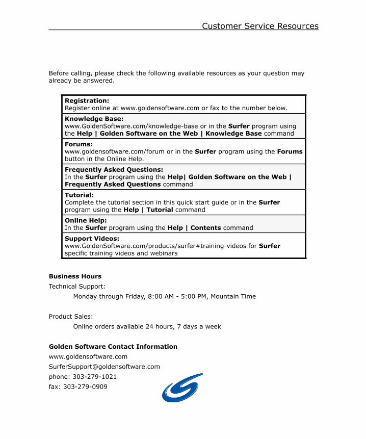
Customer Service Resources

Before calling, please check the following available resources as your question may already be answered.

Business HoursTechnical Support: Monday through Friday, 8:00 AM - 5:00 PM, Mountain Time

Product Sales: Online orders available 24 hours, 7 days a week

Golden Software Contact Informationwww.goldensoftware.comSurferSupport@goldensoftware.comphone: 303-279-1021fax: 303-279-0909

Registration: Register online at www.goldensoftware.com or fax to the number below.

Knowledge Base: www.GoldenSoftware.com/knowledge-base or in the Surfer program using the Help | Golden Software on the Web | Knowledge Base command

Forums: www.goldensoftware.com/forum or in the Surfer program using the Forums button in the Online Help.

Frequently Asked Questions: In the Surfer program using the Help| Golden Software on the Web | Frequently Asked Questions command

Tutorial: Complete the tutorial section in this quick start guide or in the Surfer program using the Help | Tutorial command

Online Help: In the Surfer program using the Help | Contents command

Support Videos: www.GoldenSoftware.com/products/surfer#training-videos for Surfer specific training videos and webinars

www.goldensoftware.com

© Copyright 2015 Golden Software, LLC. All Rights Reserved. Golden Software®, the Golden Software® mark, Surfer® and the Surfer® logo marks are owned by Golden Software and may be registered. All other trademarks and logos are the property of their respective companies. Software developed in the USA.

Golden Software, LLC809 14th StreetGolden, Colorado 80401 USA

Phone +1 303 279 1021Fax +1 303 279 0909

www.goldensoftware.com

Surfer - sciencesoftware.cz fileUninstalling Surfer 3 A Note about the Documentation 3 Three-Minute...

Documents

Transcript of Surfer - sciencesoftware.cz fileUninstalling Surfer 3 A Note about the Documentation 3 Three-Minute...