Supremal Multiscale Signal Analysis

8/9/2019 Supremal Multiscale Signal Analysis

http://slidepdf.com/reader/full/supremal-multiscale-signal-analysis 1/27

SUPREMAL MULTISCALE SIGNAL ANALYSIS∗

ULISSES BRAGA-NETO† AND JOHN GOUTSIAS‡

SIAM J. MATH. ANAL. c 2004 Society for Industrial and Applied MathematicsVol. 36, No. 1, pp. 94–120

Abstract. We introduce a novel approach to nonlinear signal analysis, which is referred to assupremal multiscale analysis. The proposed approach provides a rigorous mathematical foundationfor a class of nonlinear multiscale signal analysis schemes and leads to a decomposition that caneffectively be used in signal processing and analysis. Moreover, it is related to the supremal scale-spaces proposed by Heijmans and van den Boomgaard and is similar in flavor to the well-knownlinear multiresolution theory of Mallat and Meyer. In this framework, linear concepts such as vectorspaces, projections, and linear operators are replaced by conceptually analogous nonlinear notions.

We use supremal multiscale analysis to construct a multiscale image decomposition scheme basedon two mathematical concepts that play a key role in the analysis and interpretation of images byvision systems, namely, regional maxima and connectivity. The resulting scheme is referred to asskyline supremal multiscale analysis and satisfies several useful properties desired by any multiscaleimage analysis tool. It is grayscale invariant, as well as translation and scale invariant. Moreover,it progressively removes connected components from the level sets of an image without introducingnew ones. But, most importantly, it decomposes the regional maxima of an image in a natural causalhierarchy by gradually removing these maxima without introducing new ones.

Image decomposition by skyline supremal multiscale analysis can be used to construct nonlinear

tools for image processing and analysis that provide solutions to problems where traditional lineartechniques are ineffective. We discuss one such tool and illustrate its use in ob ject-based extractionand denoising.

Key words. complete lattices, connectivity, connected operators, mathematical morphology,multiscale signal approximation, multiscale signal analysis, nonlinear signal analysis, scale-spaces,object-based image analysis

AMS subject classifications. 68U10, 94A08, 94A12

DOI. 10.1137/S0036141002409945

1. Introduction. An important methodology for signal processing and analysisrepresents a signal at multiple scales. This methodology is based on the fundamen-tal observation that information pertaining to features of interest in a signal is not

confined to a particular scale, but it may span several scales. In order to effectivelycharacterize such information, it is necessary to gradually simplify the signal, bymeans of a scale-dependent operator, which monotonically removes features of inter-est as the scale increases. The resulting evolution of a signal from fine to coarse scalesis known as a scale-space (e.g., see [1, 2, 18, 21, 22, 42]).

Although early scale-space techniques were based on linear operators, it has beenincreasingly recognized that these techniques severely limit the capability of scale-spaces to accurately represent features of interest at coarser scales. For this reason,scale-space techniques based on nonlinear operators (or nonlinear partial differentialequations) have appeared in the literature (e.g., see [1, 2, 32, 38, 41]). It is noticeable

∗Received by the editors June 20, 2002; accepted for publication (in revised form) October 10,2003; published electronically June 22, 2004. This work was supported by the Office of Naval

Research, Mathematical, Computer, and Information Sciences Division, under ONR grants N00014-90-1345 and N00014-01-1-0027.

http://www.siam.org/journals/sima/36-1/40994.html†Section of Clinical Cancer Genetics, University of Texas MD Anderson Cancer Center, Houston,

TX 77030 and Department of Electrical Engineering, Texas A&M University, College Station, TX77840 ([email protected]). This author was supported by the CNPq Scholarship 200725196-3 of the Brazilian government.

‡Center for Imaging Science and Department of Electrical and Computer Engineering, The JohnsHopkins University, Baltimore, MD 21218 ([email protected]).

94



SUPREMAL MULTISCALE SIGNAL ANALYSIS 95

that several of these techniques are based on morphological operators [1, 2, 3, 8, 9, 10,15, 17, 28, 29, 37, 38].

On the other hand, a popular approach for multiscale signal processing and anal-ysis is based on the multiresolution theory of Mallat [23, 24, 25] and Meyer [30].

According to this approach, approximations of a given signal at various scales (orresolutions) can be computed by means of orthogonal projections of the signal on asequence of approximation spaces. The signal is then represented by means of a coarseapproximation plus added details. The details are computed by means of orthogonalprojections of the given signal on a sequence of detail spaces, with the detail spacesbeing orthogonal complements to the corresponding approximation spaces. At finerscales, the approximation error tends to zero, and a signal is spanned by spaces of successive details at all resolutions. This approach has naturally led to popular tech-niques for signal processing and analysis based on wavelet decompositions and filterbanks (e.g., see [25, 39]).

The basic assumption behind the multiresolution theory of Mallat and Meyeris that signals reside in a vector space (namely, the space L2(R) of finite energyfunctions), with the approximation and detail spaces being subspaces of this vectorspace. Therefore, the theory is applied to linear multiscale tools for signal analysis. Anattempt to conceptualize this approach in a nonlinear setting has appeared in [13, 14].However, the discussion in [13, 14] on this issue is only preliminary.

To accomplish this goal, it is necessary (among other things) to extend linearconcepts such as vector spaces, orthogonal projections, orthogonal spaces, and linearoperators to a nonlinear setting. One way to do this is to assume that the signal spaceis a complete lattice (i.e., a nonempty collection of partially ordered elements such thatany subcollection has a supremum and an infimum [4]). Complete lattices form thealgebraic foundation of mathematical morphology [16], which assumes that signalsare not combined by means of numerical addition and subtraction but by meansof supremum and infimum. In mathematical morphology, an operator is “linear”if it commutes over suprema or infima. In the former case, the operator is called a

dilation , whereas, in the latter case, it is called an erosion . Many linear concepts, suchas convolution, can be recast in terms of suprema and infima (e.g., see [12, 26, 27]).

In this paper, we introduce a novel approach to nonlinear signal analysis thatprovides a rigorous mathematical foundation for a class of nonlinear multiscale signalanalysis schemes and leads to a decomposition that can effectively be used for sig-nal processing and analysis. The proposed approach, which we refer to as supremal multiscale analysis , is related to the supremal scale-spaces proposed by Heijmans andvan den Boomgaard in [15] and is similar in flavor to the well-known linear multires-olution theory of Mallat and Meyer. In this framework, vector spaces are replacedby sup-closed spaces, projections are replaced by idempotent operators, orthogonalprojections are replaced by sup-projections, orthogonal spaces are replaced by sup-orthogonal spaces, and linear operators are replaced by morphological operators.

We use supremal multiscale analysis to construct a multiscale image decomposi-tion scheme, based on morphological reconstruction operators, which selectively re-moves regional maxima from a signal. Perhaps the most important feature of theproposed scheme, which is referred to as skyline supremal multiscale analysis , is itsconstruction by means of two mathematical concepts that play a key role in the anal-ysis and interpretation of images by vision systems, namely, regional maxima andconnectivity (e.g., see [17, 20, 34]). This scheme represents a signal as the supremumof a coarse approximation and details. The coarse approximation preserves regional



96 ULISSES BRAGA-NETO AND JOHN GOUTSIAS

maxima that are at some level σ or above, while it flattens the rest. In addition, thedetails preserve regional maxima with values in nonoverlapping subintervals of (0 , σ)and flatten the rest. The skyline supremal multiscale analysis is shown to satisfya number of useful properties desired by any multiscale signal analysis tool. It is

grayscale, translation, and scale invariant. Moreover, it progressively removes con-nected components from the level sets of a signal without introducing new ones. But,most importantly, it decomposes the regional maxima of a signal in a natural causalhierarchy by gradually removing these maxima without introducing new ones.

Image decomposition by skyline supremal multiscale analysis can be used to con-struct nonlinear tools for image processing and analysis that can provide solutionsto some problems where traditional linear techniques are ineffective. We discuss onesuch tool and illustrate its effectiveness in object-based extraction and denoising.

This paper is structured as follows. In section 2, we provide a brief overview of basic mathematical concepts used throughout the paper and introduce our notation.In section 3, we introduce our framework for nonlinear multiscale analysis, which leadsto the concepts of supremal multiscale approximation and supremal multiscale anal-ysis. We also establish a relationship between the supremal multiscale approximation

and scale-spaces and present two binary examples that illustrate these concepts. Insection 4, we present the skyline supremal multiscale analysis scheme, constructedby means of morphological reconstruction operators, which decomposes the regionalmaxima of a signal in a natural causal hierarchy by selectively removing these maximawithout introducing new ones. We show that the proposed scheme is indeed a supre-mal multiscale analysis, and we study its main properties. In section 5, we presentexamples that illustrate the use of the proposed multiscale approach in two imageprocessing and analysis problems: object-based extraction and denoising. In the firstcase, the skyline supremal multiscale decomposition scheme is used to extract objectsof interest, by placing them on individual frames, and enhance their presence by sup-pressing (flattening) surrounding details. In the second case, the scheme is used torestore an image corrupted by structured (more than a pixel thick) “pepper” noise.Finally, we summarize our conclusions in section 6.

2. Mathematical preliminaries. In this section, we review basic mathemati-cal concepts and introduce our notation. For a more detailed exposition, the readeris referred to [4, 5, 6, 7, 16, 35, 36].

A partially ordered set or, briefly, a poset , is a nonempty set furnished with abinary partial order relation ≤ (i.e., a binary order relation that is reflexive, antisym-metric, and transitive). A complete lattice (L, ≤) is a poset such that every familyM ⊆ L has an infimum

M and a supremum

M in L. Every complete lattice

(L, ≤) has a least element O and a greatest element I , given by O =

L and I =

L,respectively. In this paper, whenever we use the term “lattice” we mean “completelattice.” In addition, we often refer to “lattice L” when there is no confusion as tothe underlying partial order.

The following are some examples of lattices.

Example 1.(a) The collection P (E ) of all subsets of a set E , with set inclusion as the par-

tial order. The infimum and supremum are set intersection and set union,respectively. This lattice is used as a mathematical model for binary imagesdefined on E .

(b) The collection G (Rd) of all open subsets of the Euclidean space Rd, with setinclusion as the partial order. The infimum is the topological interior of set




intersection, whereas the supremum is set union. This lattice can also be usedas a mathematical model for binary images on E . In this case, it is assumedthat images do not include their boundary.

(c) The set R = R ∪ {−∞, ∞} of extended real numbers and the set Z = Z ∪

{−∞, ∞} of extended integers, as well as any closed subinterval of those,with the usual numerical ordering as the partial order. The infimum andsupremum are given by the usual numerical infimum and supremum. Theseare chains (i.e., totally ordered lattices), which are used for modeling imagevalues.

(d) The collection Fun(E, T ) of all functions from a set E into a lattice T , withthe partial order f ≤ g if f (v) ≤T g(v), for all v ∈ E , where “≤T ” is thepartial order relation on T . The infimum and supremum are the pointwiseinfimum and supremum, given, respectively, by (

f α)(v) =

f α(v) and

(

f α)(v) =

f α(v), for all v ∈ E , where the infimum and supremum onthe right-hand side are in T . When T is a chain, this lattice is used as amathematical model for grayscale images defined on E .

(e) The collection Funu(E, T ) of all upper semicontinuous (u.s.c.) functions [19]from a topological space E into a lattice T , with the partial order f ≤ gif f (v) ≤T g(v), for v ∈ E . The infimum is the usual pointwise infi-mum, given by (

uf α)(v) =

f α(v), for v ∈ E . However, the supremum

is given by (uf α) (v) =

{t ∈ T | v ∈

X t(f α)}, for v ∈ E , where

X t(f ) = {v ∈ E | f (v) ≥ t} is the level set of f at level t, and A denotesthe closure of a set A [7, Prop. 4.2.6]. Nevertheless, it can be shown thatthe supremum of any finite family of u.s.c. functions corresponds to the usualpointwise supremum. In general, whenever

f α is u.s.c., then

uf α =

f α

so that the supremum in lattice Funu(E, R) can, and often does, reduce tothe usual pointwise supremum. When T is a chain, this lattice is also usedas a mathematical model for grayscale images defined on E . In this case,however, images are assumed to satisfy the property of upper semicontinuity.

The level sets of a function f ∈ Fun(E, T ) satisfy the following properties:(a) X t(f ) ⊆ X s(f ) if t ≥ s; (b) f ≤ g if and only if X t(f ) ⊆ X t(g) for all t ∈ T (inparticular, f = g if and only if X t(f ) = X t(g) for all t ∈ T ); (c) for t ∈ T , we havethat X t(

f α) =

X t(f α), whereas X t(

f α) =

X t(f α) if {f α} is a finite family or

if T is finite; (d) f ∈ Funu(E, T ) if and only if the sets X t(f ) are closed in E for allt ∈ T .

Given a family M ⊆ L, we denote by M | ∨ the family sup-generated by M,i.e., the family consisting of all elements of L that are obtained by taking suprema of elements of M. The family M is said to be sup-closed if M = M | ∨ (in particular,M must be nonempty, since O =

∅ ∈ M).

A subset S of a lattice L is called a sup-generating family for L if every elementof L can be written as the supremum of elements in S ; i.e., L = S | ∨ . An elementof the sup-generating family S is called a sup-generator . It is assumed here that O is

not a sup-generator; i.e., O /∈ S . For example, the lattice P (E ) of binary images issup-generated by the points in E . We define the family S (A) = {x ∈ S | x ≤ A} forA ∈ L. Clearly, A is sup-generated by S (A).

An operator ψ on a lattice L is a mapping ψ : L → L. The invariance domain of ψ is defined as Inv(ψ) = {A ∈ L | ψ(A) = A}. An operator ψ is said to be increasing ,if A ≤ B ⇒ ψ(A) ≤ ψ(B), for all A, B ∈ L; antiextensive , if ψ(A) ≤ A, for allA ∈ L; idempotent , if ψψ(A) = ψ(A), for all A ∈ L. If ψ distributes over infima,




it is called an erosion , whereas, if it distributes over suprema, it is called a dilation .If ψ is increasing, antiextensive, and idempotent, it is called an opening . It can beshown (e.g., see [33]) that if {γ α} is a family of openings, then

γ α is an opening

as well, with Inv( γ α) = Inv(γ α) | ∨ . Given a poset K, the family of openings

{γ α | α ∈ K} is a granulometry if γ α1 ≤ γ α2 for α1 ≥ α2.The translation Ah of a set A ∈ P (E ) is another set in P (E ), given by Ah = {v +

h | v ∈ A}. The translation-invariant erosion of A ∈ P (E ) by a structuring element B ∈ P (E ) is defined as B(A) = AB = {h ∈ E | Bh ⊆ A}. Similarly, the translation-invariant dilation of A by B is defined as δ B(A) = A ⊕ B =

{Bh | h ∈ A}. It can

be shown that the operator θB(A) = A ◦ B = (A B) ⊕ B =h∈E {Bh | Bh ⊆ A} is

an opening. This operator is referred to as a structural opening . If A ∈ Inv(θB), wesay that A is B -open .

An increasing operator ψ on L is said to be ↓-continuous if, for every totallyordered subset K of L that contains at most a countable number of elements, we havethat

ψ

K

=

A∈Kψ(A).

If ψ is an ↓-continuous operator on a lattice L and if {A(s) | s ∈ R} is a decreasingfamily of elements in L, then [7, Prop. 2.2.10]

(2.1) ψ

s<t

A(s)

=s<t

ψ(A(s)) ∀ t ∈ R.

Consider now a lattice L, with a sup-generating family S . A family C ⊆ L iscalled a connectivity class in L if the following conditions are satisfied:

(i) O ∈ C ;

(ii) S ⊆ C ;

(iii) for a family {C α} in C such that C α = O, we have that C α ∈ C .

The family C generates a connectivity in L, and the elements in C are said to beconnected .

Classical topological and graph-theoretic connectivities correspond to connectiv-ity classes, and so do several examples of fuzzy connectivity [5, 7]. Moreover, basedon the notion of connectivity class, many new interesting examples of connectivitycan be defined [5, 6, 7, 35, 36].

We say that C is a connected component of A ∈ L if C ∈ C , C ≤ A, andthere is no C ∈ C different from C such that C ≤ C ≤ A. In other words, aconnected component of an object is a maximal connected part of the object. Theset of connected components of A is denoted by C (A).

We can define an operator γ x(A) that extracts connected components from ele-ments A ∈ L by

γ x(A) = {C ∈ C | x ≤ C ≤ A}, A ∈ L, x ∈ S .

It can be seen that this operator is an opening; it is called the connectivity opening associated with C . It can also be checked that γ x(A) ∈ C . As a matter of fact, γ x(A)is the connected component C of A marked by x (i.e., such that x ≤ C ).

It is natural to extend connectivity openings to operators that extract connectedcomponents marked by arbitrary markers, not just sup-generators. This gives rise




f

(a)

~( | )ρ f g

(b)

g

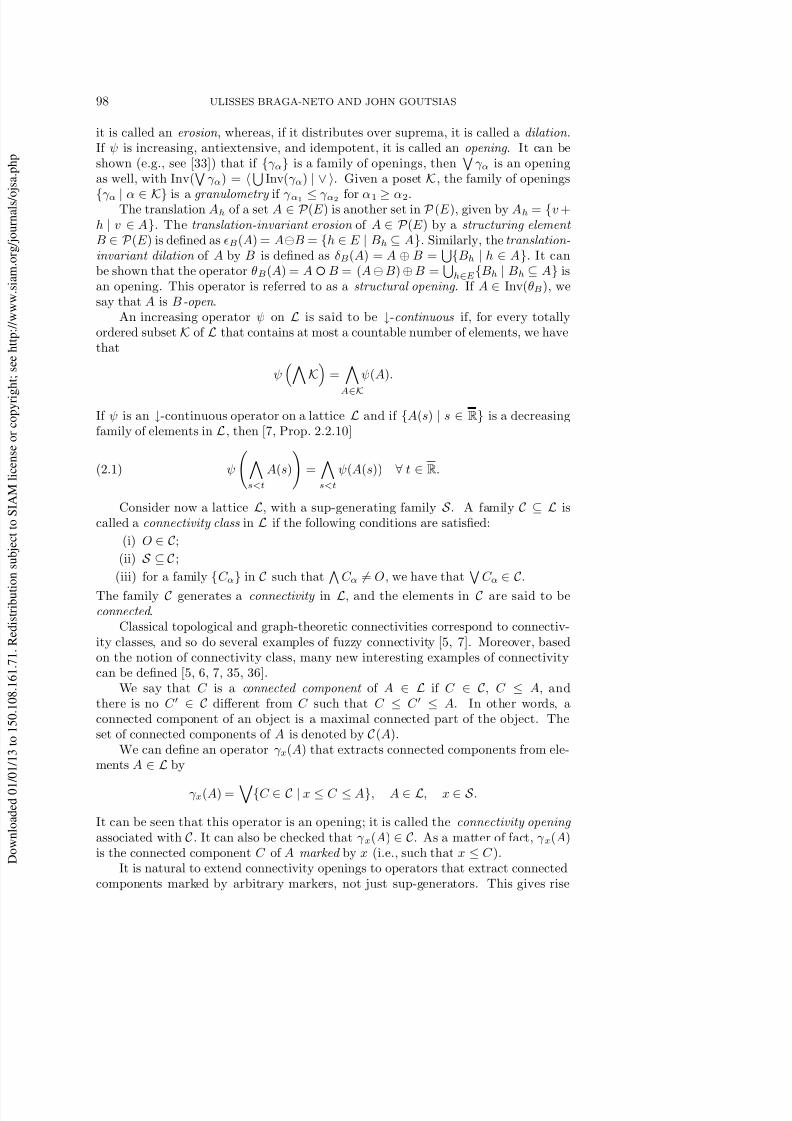
Fig. 1. (a) Original image f and a marker g. (b) The grayscale reconstruction ρ (f | g),according to the usual topological connectivity of the Euclidean real line.

to the reconstruction operator associated with a connectivity class C . For a markerM ∈ L, the reconstruction ρ(A | M ) of a given A ∈ L from M is defined by

ρ(A | M ) =

x∈S (M )γ x(A) =

{C ∈ C (A) | C ∧ M = O}.

The second equality above can be easily verified [6, 7]. Hence, the reconstructionoperator ρ(A | M ) extracts the connected components of A that “intersect” marker M .Being a supremum of openings, the operator ρ(· | M ) is an opening on L for a fixedmarker M ∈ L. When M reduces to a sup-generator x, the reconstruction ρ(A | x)reduces to the connectivity opening γ x(A), provided that x ≤ A.

Given a connectivity class C in the binary lattice P (E ) and the associated recon-struction operator ρ: P (E )×P (E ) → P (E ), we can define an operator ρ: Fun(E, T )×Fun(E, T ) → Fun(E, T ) by

(2.2)

ρ (f | g)(v) =

{t ∈ T | v ∈ ρ(X t(f ) | X t(g))}, v ∈ E.

It can be shown that ρ (· | g) is an opening on Fun(E, T ) for a fixed marker g ∈Fun(E, T ). If we assume that T is a chain, then the operator ρ(f | g) in (2.2) is knownas the grayscale reconstruction of f from marker g associated with the connectivityclass C . The grayscale reconstruction is a very useful operator in applications [40].Figure 1 illustrates the grayscale reconstruction operator in the one-dimensional case.

3. Supremal scale-spaces and multiscale analysis. In this section, we in-troduce a framework for nonlinear multiscale signal analysis, which is related to thesupremal scale-spaces introduced by Heijmans and van den Boomgaard [15]. The pro-posed framework is referred to as supremal multiscale analysis and leads to a nonlinearmultiscale signal representation scheme that decomposes a signal into the supremumof a coarse approximation and details. We show that supremal multiscale analysissatisfies a number of properties, which are similar in flavor to properties satisfied bythe well-known linear multiresolution signal analysis scheme of Mallat [23, 24, 25] andMeyer [30]. As a matter of fact, we derive the supremal multiscale analysis scheme byusing nonlinear analogues of certain linear concepts (e.g., vector spaces, orthogonalprojections, and orthogonal complements).

We assume that signals of interest reside in a complete lattice (V , ≤). An operatorφ on V is said to be a projection if it is idempotent [14, 31]. Furthermore, we say thatφ is a projection on U ⊆ V if Ran(φ) = U and φ is idempotent on U (in which caseInv(φ) = Ran(φ) = U ), where Ran(φ) denotes the range of operator φ. In the linear




multiresolution framework proposed in [23, 24, 25, 30], approximations of signalsat various scales are computed by means of orthogonal projections on a sequenceof approximation spaces. An orthogonal projection of a signal f ∈ V on a vectorsubspace U ⊆ V is defined as the signal φ(f ) ∈ U that minimizes the norm f − g

over all signals g ∈ U . Note that the range of this operator is U and that the operatoris idempotent; therefore, it is a projection on U . In the nonlinear framework proposedhere, V is not a vector space in general. Therefore, we introduce the alternative notionof sup-projection, which is conceptually analogous to an orthogonal projection.

Definition 3.1. Let U ⊆ V such that U is sup-closed in V . The operator

(3.1) φ(f ) =

{g ∈ U | g ≤ f }, f ∈ V ,

defines the sup-projection of f on U .The sup-closure requirement and (3.1) imply that Ran(φ) = U and that φ is idem-

potent on U ; therefore, φ is a projection on U . The requirement that U must besup-closed is analogous to the linear requirement that U must be a vector space (i.e.,closed under linear combinations). Note that (3.1) implies that φ(f ) is the “closest”

element to f in U , in the sense of the underlying partial order. Hence, a sup-projectionis a nonlinear analogue of an orthogonal projection.

A fundamental aspect of (linear) multiresolution analysis is that distinct signalapproximations can be obtained from each other by means of scaling (this is knownas the “dilation” property). In order to formulate this idea in a nonlinear setting, weuse a general definition of scaling, proposed in [15]. In what follows, id denotes theidentity operator.

Definition 3.2. A family S = {st | t ∈ (0, ∞)} of operators on a lattice V is a scaling if

(i) s1 = id,(ii) srst = srt for r, t ∈ (0, ∞).This definition implies that S is a commutative group, where the inverse s−1t of

st is given by s−1

t = s1/t for t ∈ (0, ∞). Moreover, if S = {st | t ∈ (0, ∞)} is a scalingon V , then so is S p = {stp | t ∈ (0, ∞)}, p ∈ R [15].Example 2.

(a) For V = P (Rd), the scaling {tA | t ∈ (0, ∞)}, where tA = {tv | v ∈ A}, forA ∈ V , is known as the spatial scaling .

(b) For V = Fun(E, R), the scalings {tf (·) | t ∈ (0, ∞)}, {f (·/t) | t ∈ (0, ∞)},and {tf (·/t) | t ∈ (0, ∞)} are known as the gray-level , spatial , and umbral scalings , respectively.

In practice, useful scalings consist of increasing operators. We refer to these asincreasing scalings . For example, all scalings considered in Example 2 are increasing.The following result shows that scalings are increasing if and only if they consist of dilations.

Proposition 3.3. A scaling S = {st | t ∈ (0, ∞)} on a lattice V is increasing if

and only if st is a dilation for every t ∈ (0, ∞).Proof . The reverse implication follows trivially from the fact that every dilation

is an increasing operator [16]. We show the direct implication. Given t ∈ (0, ∞) and{f α} ⊆ V , we have that st(

f α) ≥

st(f α), since st is increasing. To show the

reverse inequality, note that s−1t (

st(f α)) ≥

s−1t st(f α) =

f α, since s−1t = s1/tis increasing. Applying st on both sides of this inequality gives sts

−1t (

st(f α)) =st(f α) ≥ st(

f α). Therefore, st(

f α) =

st(f α), and st is a dilation on V .




We now introduce an axiomatic formulation for supremal multiscale approxima-tions, which compute approximations of signals at various scales by means of sup-projections on a sequence of approximation spaces.

Definition 3.4. Let S be a scaling on a lattice V . A family {V σ | σ ∈ (0, ∞)}

of sup-closed subsets of V is said to be a supremal multiscale S -approximation of V if the following properties are satisfied:

1. The sequence {V σ | σ ∈ (0, ∞)} is decreasing; i.e.,

(3.2) V τ ⊆ V σ for τ ≥ σ.

This implies that an approximation at scale σ contains all necessary infor-mation to compute an approximation at a coarser scale τ ≥ σ.

2. The sequence {V σ | σ ∈ (0, ∞)} “converges” to V , as σ → 0+, in the sense that

(3.3) limσ→0+

V σ

σ∈(0,∞)

V σ | ∨

= V .

This implies that any signal can be recovered by the supremum of its approx-imations at sufficiently small scales.

3. ( S -invariance). We have that

(3.4) f ∈ V σ ⇔ sτ/σ(f ) ∈ V τ for σ, τ ∈ (0, ∞).

This means that an approximation space V σ can be obtained from another approximation space V τ , and vice-versa, by means of scaling.

The previous properties are similar in flavor to properties satisfied by the linearmultiresolution analysis scheme of Mallat and Meyer. The approximation of a signalf ∈ V at scale σ ∈ (0, ∞) is given by the sup-projection of f on the approximationspace V σ, which therefore must be sup-closed. This is the nonlinear analogue of the assumption that the approximation spaces are vector subspaces. The inclusionproperty specified by (3.2) is also true in the linear case. The convergence requirementspecified by (3.3) is similar to the one in the linear case, except that linear closure isreplaced by sup-closure. Finally, the scaling requirement specified by (3.4) is similarto the one in the linear case. However, a very important property of the linear caseis the existence of vector bases for the approximation spaces. This is an inherentlylinear property and has no counterpart in a nonlinear setting.

Note that the sup-closure assumption implies that, for σ ∈ (0, ∞), V σ is a completelattice under the partial order of V [16, Prop. 2.12]. The proof of the following resultis straightforward.

Proposition 3.5. The family {V σ | σ ∈ (0, ∞)} is a supremal multiscale S -approximation of V if and only if the family {V σp | σ ∈ (0, ∞)}, p ∈ R, is a supremal multiscale S p-approximation of V .

For each σ ∈ (0, ∞), let us define the approximation operator φσ on V as theoperator that maps an element f ∈ V to its sup-projection on V σ; i.e.,

(3.5) φσ(f ) =

{g ∈ V σ | g ≤ f }, f ∈ V , σ ∈ (0, ∞).

The operator φσ provides the approximation of a signal in V at scale σ. The followingfundamental result implies that a supremal multiscale approximation can be specifiedby its approximation operators.




Proposition 3.6. Let {V σ | σ ∈ (0, ∞)} be a supremal multiscale S -approximation of V , where S is an increasing scaling. The family {φσ | σ ∈ (0, ∞)} of approximation operators is such that Inv(φσ) = V σ, for σ ∈ (0, ∞), and

(i) the family {φσ | σ ∈ (0, ∞)} is a granulometry on V ,

(ii) σ∈(0,∞) φσ = id,(iii) φσ = sσ/τ φτ s

−1σ/τ

for σ, τ ∈ (0, ∞).

Conversely, if {φσ | σ ∈ (0, ∞)} is a family of operators on V that satisfies the pre-vious properties (i)–(iii), then {V σ = Inv(φσ) | σ ∈ (0, ∞)} is a supremal multiscale S -approximation of V , with approximation operators that coincide with {φσ | σ ∈ (0, ∞)}.

Proof . For f ∈ Inv(φσ), we have that f = φσ(f ) =

{g ∈ V σ | g ≤ f } ⇒f ∈ V σ | ∨ = V σ, since V σ is sup-closed, so that Inv(φσ) ⊆ V σ. The reverseinclusion follows easily from (3.5); hence, Inv(φσ) = V σ. We now show (i). From(3.5), it is clear that φσ is increasing and antiextensive. This implies that φσφσ ≤φσ. On the other hand, (3.5) implies that g ∈ V σ, g ≤ f ⇒ g ≤ φσ(f ) so thatφσ(f ) =

{g ∈ V σ | g ≤ f } ≤

{g ∈ V σ | g ≤ φσ(f )} = φσφσ(f ) for f ∈ V .

Therefore, φσ is idempotent, and hence it is an opening. For τ ≥ σ, we have that

Inv(φτ ) = V τ ⊆ V σ = Inv(φσ), which implies that φτ ≤ φσ [16, Thm. 3.24]. Therefore,{φσ | σ ∈ (0, ∞)} is a granulometry on V . To show (ii), we use the fact that thesupremum

θα of openings is an opening, with Inv(

θα) =

Inv(θα) | ∨ . Hence,

Inv(σ∈(0,∞) φσ) =

σ∈(0,∞) Inv(φσ) | ∨ =

σ∈(0,∞) V σ | ∨ = V = Inv(id). But,

since id is an opening and two openings are equal if and only if their domains of invariance are equal [16, Thm. 3.24], we get that

σ∈(0,∞) φσ = id. We now show (iii).

For f ∈ V , we have that φσ(f ) =

{g ∈ V σ | g ≤ f } =

{sσ/τ (h) | h ∈ V τ , sσ/τ (h) ≤

f } = sσ/τ (

{h | h ∈ V τ , h ≤ s−1σ/τ (f )}) = sσ/τ φτ s−1σ/τ (f ), since sσ/τ is a dilation (see

Proposition 3.3). Therefore, φσ = sσ/τ φτ s−1σ/τ for σ, τ ∈ (0, ∞).

We now show the converse implication. Note that, for each σ ∈ (0, ∞), V σ =Inv(φσ) is sup-closed, since φσ is an opening. Equation (3.2) follows from the factthat φσ ≤ φτ for σ ≥ τ [16, Thm. 3.24]. Equation (3.3) follows from V = Inv(id) =

Inv(σ∈(0,∞) φσ) = σ∈(0,∞) V σ | ∨ . To verify (3.4), note that f ∈ V σ ⇔ f =φσ(f ) = sσ/τ φτ s−1σ/τ (f ) ⇔ sτ/σ(f ) = φτ sτ/σ(f ) ⇔ sτ/σ(f ) ∈ V τ for σ, τ ∈ (0, ∞).

Finally, if {φσ | σ ∈ (0, ∞)} are the approximation operators associated with {V σ |σ ∈ (0, ∞)}, then Inv(φσ) = V σ = Inv(φσ) ⇔ φσ = φσ for σ ∈ (0, ∞) (see [16,Thm. 3.24]).

The following proposition shows that we can build supremal multiscale approxi-mations by using unions of existing ones.

Proposition 3.7. Let S be an increasing scaling. If, for each α, {V ασ | σ ∈(0, ∞)} is a supremal multiscale S -approximation of V , with approximation operators {φασ | σ ∈ (0, ∞)}, then {

α V ασ | ∨ | σ ∈ (0, ∞)} is a supremal multiscale S -

approximation of V as well, with approximation operators {α φασ | σ ∈ (0, ∞)}.

Proof . Equations (3.2) and (3.3) are easy to show; therefore, we show only (3.4).Let V σ = α V ασ | ∨ for σ ∈ (0, ∞). For f ∈ V σ, we have that f = f β, where eachf β belongs to some V ασ . Therefore, sτ/σ(f β) ∈ V τ , for each β and τ ∈ (0, ∞). Since V τ is sup-closed and since sτ/σ is a dilation (see Proposition 3.3), we have that sτ/σ(f ) =sτ/σ(

f β) =

sτ/σ(f β) ∈ V τ , as required. Now let φσ be the approximation operator

associated with V σ. Since Inv(φασ) = V ασ , we have that Inv(φσ) = V σ = α V ασ | ∨ =

Inv(α φασ). Since two openings are equal if and only if their domains of invariance are

equal [16, Thm. 3.24] and since α φασ is an opening, we conclude that φσ =

α φασ ,

as required.




To illustrate the concept of supremal multiscale approximation, we now providetwo binary examples. A grayscale supremal multiscale approximation scheme will bediscussed in the next section.

Example 3.

(a) Let V = G (Rd

) be the lattice of open subsets of the Euclidean space, andconsider the spaces

(3.6) V σ = {A ∈ V | A is σB-open}, σ ∈ (0, ∞),

where B ∈ V is a bounded convex structuring element (e.g., an open ball of unit radius). In (3.6), σB = {σb | b ∈ B }. The family {V σ | σ ∈ (0, ∞)} isa supremal multiscale S -approximation of V , where S is the spatial scaling:V σ is sup-closed, for σ ∈ (0, ∞), and (3.2) and (3.4) are clearly satisfied,whereas (3.3) follows from the facts that B = {(σB)v | v ∈ Rd, σ ∈ (0, ∞)} ⊂σ∈(0,∞) V σ and B is a basis for the Euclidean topology. In this case, the

approximation operators are the structural openings

φσ(A) = A ◦ σB, A ∈ V , σ ∈ (0, ∞).

(b) Let V = G (Rd), furnished with a connectivity class C , and consider the opening by reconstruction operators :

(3.7) φσ(A) = ρ(A | A ◦ σB), A ∈ V , σ ∈ (0, ∞),

where B ∈ V is a bounded structuring element. It can be shown that theinvariance domain of φσ is given by

(3.8) V σ(A) = {A ∈ V | C ◦ σB = ∅ ∀ C ∈ C (A)}, σ ∈ (0, ∞).

The family {V σ | σ ∈ (0, ∞)} is a supremal multiscale S -approximation of V ,where S is the spatial scaling. Properties (i) and (iii) of Proposition 3.6 areclearly satisfied. Now we have that φσ(A) = {C ∈ C (A) | C ∩ (A σB) =

∅} = {C ∈ C (A) | ∃ v ∈ C such that (σB)v ⊆ A}. Since A is open, for anyC ∈ C (A) and v ∈ C , we can find a σ such that (σB)v ⊆ A so that C ⊆ φσ(A).It then follows that A =

σ∈(0,∞) φσ(A), which shows property (ii). The

approximation operators {φσ | σ ∈ (0, ∞)} are, of course, given by (3.7).We now show that supremal multiscale approximations and scale-spaces are re-

lated. The following definition introduces the notion of supremal scale-space in theterminology of [15].

Definition 3.8. Let V be a lattice, and let S be a scaling on V . A family {φσ | σ ∈ (0, ∞)} of operators on V is said to be a supremal S -scale-space if

(i) φσφτ = φσ∨τ for σ, τ ∈ (0, ∞),(ii) φσsσ = sσφ1 for σ ∈ (0, ∞).We have the following result.Proposition 3.9. Let {V σ | σ ∈ (0, ∞)} be a supremal multiscale S -approximation

of V , where S is an increasing scaling. The family {φσ | σ ∈ (0, ∞)} of approximation operators, given by (3.5), is a supremal S -scale-space.

Proof . Properties (i) and (ii) of a supremal scale-space follow directly from prop-erties (i) and (iii) in Proposition 3.6.

Therefore, given a signal f ∈ V , its approximations {φσ(f ) | σ ∈ (0, ∞)} forma scale-space, where increasing scale corresponds to an “evolution” of f towards de-creasing levels of “detail.” Several scale-spaces that coincide with or are similar to the




two binary supremal multiscale approximation schemes of Example 3 have appearedin [3, 8, 9, 10, 15, 17, 28, 29, 37].

We now proceed to derive a nonlinear multiscale signal analysis scheme based onsupremal multiscale approximations.

In linear orthogonal wavelet decomposition schemes, given two approximationspaces V σ+1 ⊆ V σ, one defines a detail space W σ+1 (also called a wavelet space ) as theorthogonal complement of V σ+1 in V σ, given by

(3.9) W σ+1 = {f ∈ V σ | f ⊥ V σ+1}.

From the fact that V σ and V σ+1 are vector spaces, it follows that W σ+1 is a vectorspace as well. Moreover, W σ+1 ⊆ V σ and W σ+1 ⊥ V σ+1.

In vector analysis, a space V is said to be the direct sum of two subspaces V 1and V 2, which is denoted by V = V 1 ⊕ V 2, if

(3.10) V = {f + g | f ∈ V 1 and g ∈ V 2} and V 1 ∩ V 2 = {O}.

A fundamental property of linear wavelet analysis is that V σ = V σ+1 ⊕ W σ+1; i.e., theapproximation space at scale σ is the direct sum of the approximation and detail spacesat scale σ + 1 (which, in this case, is also an orthogonal sum, since W σ+1 ⊥ V σ+1).

In order to formulate similar ideas in a nonlinear setting, we need to define non-linear analogues of the notions of “orthogonal complement” and “direct sum.” Asignal f is said to be sup-orthogonal to a sup-closed space V if its sup-projection onV is O . Therefore, a signal f is sup-orthogonal to an approximation space V σ if andonly if φσ(f ) = O. A space W is said to be sup-orthogonal to V if every signal in W issup-orthogonal to V . Note that this implies that W and V cannot have any commonelements other than {O}. Given two approximation spaces V σ and V τ , with τ > σ,we define a detail space W σ,τ as the sup-orthogonal complement of V τ in V σ, given by

(3.11) W σ,τ = {f ∈ V σ | φτ (f ) = O}, τ > σ.

Note that this is the nonlinear analogue of (3.9). Moreover, we say that a space V isthe direct sup-sum of two subspaces V 1 and V 2, which we denote by V = V 1 ∨ V 2, if

V = V 1 ∪ V 2 | ∨ and V 1 ∩ V 2 = {O}.

This is the analogue of (3.10), where vector summation is replaced by supremum.

We now have the following definition.

Definition 3.10. Let {V σ | σ ∈ (0, ∞)} be a supremal multiscale S -approximation of V . If the detail spaces W σ,τ , given by (3.11), satisfy the property

(3.12) V σ = V τ ∨ W σ,τ for σ ∈ (0, ∞), τ ∈ (σ, ∞),

then {V σ, W σ,τ | σ ∈ (0, ∞), τ ∈ (σ, ∞)} is said to be a supremal multiscale S -analysisof V .

It follows that, in a supremal multiscale analysis, for every σ ∈ (0, ∞), τ ∈ (σ, ∞),we have that

(a) V τ , W σ,τ ⊆ V σ,(b) W σ,τ is sup-orthogonal to V τ ,(c) V σ is the direct sup-sum of V τ and W σ,τ .




These properties are the nonlinear analogues of similar properties satisfied by theapproximation and detail spaces in linear orthogonal wavelet analysis.

Next, we define the notion of detail operator.Definition 3.11. Let {V σ, W σ,τ | σ ∈ (0, ∞), τ ∈ (σ, ∞)} be a supremal multi-

scale S -analysis of V . If ψσ,τ is a projection on W σ,τ and

(3.13) φσ = φτ ∨ ψσ,τ for σ ∈ (0, ∞), τ ∈ (σ, ∞),

then {ψσ,τ | σ ∈ (0, ∞), τ ∈ (σ, ∞)} is a family of detail operators of the supremal multiscale S -analysis.

From (3.13), it follows that an approximation φσ(f ) of a signal f ∈ V can bedecomposed, in a unique way, as the supremum of a sup-projection φτ (f ) on V τ and a projection ψσ,τ (f ) on W σ,τ . Furthermore, ψσ,τ (f ) is sup-orthogonal to V τ ;i.e., φτ ψσ,τ (f ) = O. Therefore, the approximation of f at scale σ has a uniquedecomposition as the supremum of the approximation signal at scale τ and a sup-orthogonal detail signal, which contains information about f that is present at scale σbut is removed at the coarser scale τ . Finally, by applying the supremum

σ∈(0,τ ) on

both sides of (3.13) and by using properties (i) and (ii) of Proposition 3.6, we get

(3.14) f = φτ (f ) ∨σ∈(0,τ )

ψσ,τ (f ) for τ ∈ (0, ∞).

This shows that a signal f ∈ V can be uniquely decomposed in terms of a scaledsignal φτ (f ) at scale τ ∈ (0, ∞) and detail signals ψσ,τ (f ), σ ∈ (0, τ ). It is worthwhilenoticing that the decomposition suggested by (3.14) is conceptually analogous to thewell-known wavelet decomposition.

Note that, for τ ≥ τ , we have φτ ψσ,τ (f ) ≤ φτ ψσ,τ (f ) = O ⇒ φτ ψσ,τ (f ) = O .Therefore, a detail signal ψσ,τ (f ) is sup-orthogonal to all approximation spaces V τ ,τ ≥ τ .

In practice, a multiscale signal decomposition scheme can be constructed by se-lecting initial and final approximation scales σ and τ and a set of intermediary scales

σ0 = σ, σ1, . . . , σN −1, σN = τ such that σk < σk+1 for k = 0, 1, . . . , N − 1. Then, byrepeatedly applying (3.13), we get

(3.15) φσ(f ) = φτ (f ) ∨

0≤k≤N −1

ψσk,σk+1(f ), τ > σ,

which provides a decomposition of the approximation φσ(f ) of a signal f into thesequence {φτ (f ), ψσ,σ1(f ), ψσ1,σ2(f ), . . . , ψσN −1,τ (f )}. Clearly, all detail signals aresup-orthogonal to the final approximation space V τ ; i.e., φτ ψσk,σk+1(f ) = O for k =0, 1, . . . , N − 1.

Example 4.

(a) Let V = G (Rd), and consider the supremal multiscale approximation of V given in Example 3(a). Using (3.6) and (3.11), we get

W σ,τ = {A ∈ V | A ◦ σB = A and A ◦ τ B = ∅}, τ > σ.

Clearly, V σ = V τ ∪ W σ,τ | ∨ and V σ ∩ W σ,τ = {∅}. Therefore, (3.12) issatisfied so that {V σ, W σ,τ | σ ∈ (0, ∞), τ ∈ (σ, ∞)} is a supremal multiscaleS -analysis of V , where S is the spatial scaling. If B is a structuring elementthat contains the origin, then the operators

ψσ,τ (A) = A ◦ σB A τ B, τ > σ,




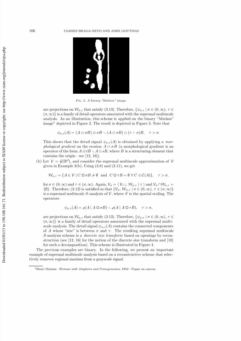
Fig. 2. A binary “Matisse” image.

are projections on W σ,τ that satisfy (3.13). Therefore, {ψσ,τ | σ ∈ (0, ∞), τ ∈(σ, ∞)} is a family of detail operators associated with the supremal multiscale

analysis. As an illustration, this scheme is applied on the binary “Matisse”image1 depicted in Figure 2. The result is depicted in Figure 3. Note that

ψσ,τ (A) = (A σB) ⊕ σB (A σB) (τ − σ)B, τ > σ.

This shows that the detail signal ψσ,τ (A) is obtained by applying a mor-phological gradient on the erosion A σB (a morphological gradient is anoperator of the form A ⊕ tB A sB, where B is a structuring element thatcontains the origin—see [12, 16]).

(b) Let V = G (Rd), and consider the supremal multiscale approximation of V given in Example 3(b). Using (3.8) and (3.11), we get

W σ,τ = {A ∈ V | C ◦ σB = ∅ and C ◦ τ B = ∅ ∀ C ∈ C (A)}, τ > σ,

for σ ∈ (0, ∞) and τ ∈ (σ, ∞). Again, V σ = V τ ∪ W σ,τ | ∨ and V σ∩W σ,τ ={∅}. Therefore, (3.12) is satisfied so that {V σ, W σ,τ | σ ∈ (0, ∞), τ ∈ (σ, ∞)}is a supremal multiscale S -analysis of V , where S is the spatial scaling. Theoperators

ψσ,τ (A) = ρ(A | A ◦ σB) ρ(A | A ◦ τ B), τ > σ,

are projections on W σ,τ that satisfy (3.13). Therefore, {ψσ,τ | σ ∈ (0, ∞), τ ∈(σ, ∞)} is a family of detail operators associated with the supremal multi-scale analysis. The detail signal ψσ,τ (A) contains the connected componentsof A whose “size” is between σ and τ . The resulting supremal multiscaleS -analysis scheme is a discrete size transform based on openings by recon-

struction (see [12, 16] for the notion of the discrete size transform and [10]for such a decomposition). This scheme is illustrated in Figure 4.

The previous examples are binary. In the following, we present an importantexample of supremal multiscale analysis based on a reconstructive scheme that selec-tively removes regional maxima from a grayscale signal.

1Henri Matisse: Woman with Amphora and Pomegranates, 1952—Paper on canvas.




ψ1 2, ( )A

ψ 2 3, ( )A

φ2 ( )A

φ3 ( )A

φ1( )A

φ4 ( )A ψ 3 4, ( )A

Fig. 3. An illustration of supremal multiscale analysis of a binary “Matisse” image A depicted in Figure 2 based on structural openings. Note that φk(A) = φk+1(A) ∪ ψk,k+1(A), for k = 1, 2, 3,and φ1(A) = φ4(A) ∪ ψ1,2(A) ∪ ψ2,3(A) ∪ ψ3,4(A), in accordance with (3.13) and (3.15). In thisexample, B is a disk structuring element of unit radius.




ψ1 2, ( )A

ψ 2 3, ( )A

φ2 ( )A

φ3 ( )A

φ1( )A

φ4 ( )A ψ 3 4, ( )A

Fig. 4. An illustration of supremal multiscale analysis of the binary “Matisse” image A depicted in Figure 2 based on openings by reconstruction. Note that φk(A) = φk+1(A) ∪ ψk,k+1(A), for k = 1, 2, 3, and φ 1(A) = φ4(A) ∪ ψ1,2(A) ∪ ψ2,3(A) ∪ ψ3,4(A), in accordance with (3.13) and (3.15).In this example, B is a disk structuring element of unit radius.




f s

t

R

X f t( )

X f s( )

Fig. 5. A signal f with a regional maximum R at level t. Note that R is a connected component of X t(f ), that R ∩ X s(f ) = ∅, for s > t, and that f is constant over R. The usual topological connectivity of the Euclidean real line is assumed.

4. Skyline supremal multiscale analysis. Recall the lattice Funu(E, T ) of u.s.c. functions, discussed in Example 1(e). Here we adopt as the lattice V of signalsof interest the lattice V = Funu(E, R+) of nonnegative u.s.c. real-valued functionsdefined on a topological space E . We are making the following basic assumption.

Assumption 1. We assume that E is a compact Hausdorff space with a countablebasis. Moreover, we assume that E is furnished with a connectivity class C ⊆ P (E )such that we have the following:

(a) A ∈ C implies that A ∈ C (in this case, the connectivity class C is said to becompatible with the topology of E [6]).

(b) The connectivity openings {γ x | x ∈ E }, associated with C , are ↓-continuousoperators on F (E ) (i.e., on the collection of all closed subsets of E ).

(c) For each A ∈ F (E ), γ x(A) is an u.s.c. function from A into F (E ).For example, one may assume E to be a connected, closed, and bounded subset

of Rd, with the Euclidean topology, and take C to be the connectivity class consistingof the usual Euclidean connected subsets of E . It has been shown in [6] that thischoice satisfies all conditions stated in Assumption 1.

Next, we give a precise definition of a regional maximum of a signal in V .Definition 4.1. A set R ⊆ E is a regional maximum of f ∈ Funu(E, R+) at

level t ∈ R+ if R is a connected component of X t(f ) and R ∩ X s(f ) = ∅ for all s > t.Therefore, regional maxima depend on the underlying connectivity assumed. See

Figure 5 for an illustration. A regional maximum is always a closed set, since X t(f )is closed and C is compatible [7]. It is easy to see that a signal f ∈ Funu(E, R+)is constant over a regional maximum R; we denote this constant value by f (R). Inaddition, we denote by R(f ) the set of all regional maxima of a signal f and by Rt(f )the set of all regional maxima of f at level t or above; i.e., Rt(f ) = {R ∈ R(f ) |f (R) ≥ t} for t ∈ R+.

We have the following result regarding regional maxima.Proposition 4.2.

(a) Any function f ∈ Funu(E, R+) has at least one regional maximum.(b) A function f ∈ Funu(E, R+) has exactly one regional maximum if and only

if X t(f ) ∈ C for all t ∈ R+.Proof . (a) From Weierstrass’s theorem of real analysis [19] and the facts that E

is compact and f is an u.s.c. function, f achieves its supremum in E ; i.e., there is a




point x0 ∈ E such that f (x0) =

{f (x) | x ∈ E }. It is clear that X t(f ) = ∅ for allt > f (x0). Hence, R = γ x0(X f (x0)(f )) is a regional maximum of f at level f (x0).

(b) We show that f has two or more regional maxima if and only if X t(f ) ∈ C ,for some t ∈ R+, which is the contrapositive of the assertion. To show the direct

implication, assume that R1 and R2 are two regional maxima of f . If f (R1) =f (R2) = t, then X t(f ) ∈ C . Otherwise, let f (R1) = t1 > t2 = f (R2). We havethat R1 ⊆ X t1(f ) ⊆ X t2(f ). But R2 ∩ X t1(f ) = ∅ ⇒ R1 ∩ R2 = ∅ so that R2 mustbe a strict subset of X t2(f ), which implies that X t2(f ) ∈ C . To show the converseimplication, assume that X t(f ) ∈ C , for some t ∈ R+, and let C 1 and C 2 be twoconnected components of X t(f ). Sets C 1 and C 2 are closed subsets of the compactspace E ; thus C 1 and C 2 are themselves compact [11]. Hence, the restrictions f 1and f 2 of f to C 1 and C 2, respectively, are u.s.c. functions defined on compact setsso that each achieves its supremum, say, at points x1 ∈ R1 and x2 ∈ R2. Clearly,the corresponding regional maxima of f 1 and f 2 at f (x1) and f (x2), respectively, aredistinct regional maxima of f .

Part (a) of the previous proposition shows that the set R(f ) of regional maximaof f is nonempty, whereas part (b) indicates that the notions of regional maxima and

connectivity of level sets are closely related.Recall from section 2 the grayscale reconstruction operator associated with a

connectivity class C ⊆ P (E ). This operator will be central for our purposes. Thenext fundamental result shows that a signal f ∈ Funu(E, R+) can be “reconstructed”from the grayscale reconstructions of f “marked” by each of its regional maxima.Before that, we need the following definition: A cylinder hA,t of base A ⊆ E andheight t ∈ R+ is a function in Funu(E, R+) defined by

hA,t(x) =

t if x ∈ A,0 otherwise

for x ∈ E .

Proposition 4.3. Let f ∈ Funu(E, R+). For each R ∈ R(f ), we have that g = ρ(f | hR,f (R)) ∈ Funu(E, R+), and R(g) = {R}, with g (R) = f (R). Moreover,

(4.1) f =u

{ρ(f | hR,f (R)) | R ∈ R(f )}.

Proof . From the definition of ρ in (2.2), we can write

(4.2) g(v) = ρ(f | hR,f (R))(v) =

{t ∈ R+ | v ∈ ρ( X t(f ) | X t(hR,f (R)))}, v ∈ E.

Note that X t(hR,f (R)) = R, if t ≤ f (R), and X t(hR,f (R)) = ∅ if t > f (R). Also,X t(f ) ∩ R = ∅ for t > f (R). Hence, ρ(X t(f ) | X t(hR,f (R))) = ρ(X t(f ) | R) for

all t ∈ R+. Moreover, R is connected so that it must be contained in one of theconnected components of X t(f ), and, therefore, ρ(X t(f ) | R) = γ x(X t(f )) for somex ∈ R. Thus, (4.2) becomes g(v) =

{t ∈ R+ | v ∈ γ x(X t(f ))} for v ∈ E . Hence,

X t(g) = s<t γ x(X s(f )) = γ x s<tX s(f ) = γ x(X t(f )), for all t ∈ R+, from the↓-continuity of γ x on F (E ) and (2.1). In other words, X t(g) is a closed (by thecompatibility of C ) connected set, for all t ∈ R+, so that, by Proposition 4.2(b), g isu.s.c. and has a single regional maximum. In addition, we have that X t(g) = R, fort = f (R), and X t(g) = ∅, for t > f (R), so that R is the only regional maximum of gat level g(R) = f (R). This shows the first part of the result. Note that the right-handside of (4.1) makes sense, since ρ(f | hR,f (R)) is a function in Funu(E, R+) for eachR ∈ R(f ). Let C be a connected component of any nonempty level set X t(f ) of f . It




follows from the fact that any closed subset of a compact space is compact and fromthe compatibility of C that C is compact. In addition, the restriction of f to C isan u.s.c. function; hence, C contains some regional maximum R ∈ Rt(f ). Moreover,the definition of regional maximum implies that each R ∈ Rt(f ) must be contained

in some component C of X t(f ). Since X t(f ) equals the union of its components, weconclude that X t(f ) =

R∈Rt(f )

ρ(X t(f ) | R). But, by definition, any R ∈ R(f )

Rt(f ) does not intersect X t(f ). Hence, X t(f ) = R∈R(f ) ρ(X t(f ) | R). In addition,

from our previous discussion, we have that X t( ρ(f | hR,f (R))) = ρ(X t(f ) | R) for all

t ∈ R+. It follows from the last two equations and the fact X t(f ) = s<t

X s(f α)

that [7]

X t

u

{ρ(f | hR,f (R)) | R ∈ R(f )}

=s<t

R∈R(f )

X t( ρ(f | hR,f (R)))

=s<t

R∈R(f )

ρ(X s(f ) | R)

= s<t

X s(f ) = s<t

X s(f ) = X t(f ),

for all t ∈ R+, which implies (4.1).Now consider the subsets V σ of V given by

(4.3) V σ = {O} ∪ {f ∈ V | R(f ) = Rσ(f )}, σ ∈ (0, ∞).

In other words, V σ consists of the least signal O and all signals whose regional maximaare at level σ or above. The following is a fundamental result for our purposes.

Proposition 4.4. The space V σ is sup-closed in Funu(E, R+) for σ ∈ (0, ∞).Proof . First, note that

∅ = O ∈ V σ for every σ ∈ (0, ∞). For a given σ ∈ (0, ∞),

let {f α} be a family of functions in Funu(E, R+) such that {f α} ⊆ V σ. We can assume,

without loss of generality, that f α = O for all α. Hence, Rσ(f α) = R(f α) = ∅, foreach f α, which implies that X t(f α) = ∅ for all t ≤ σ. Let f = uf α. We have

that X t(f ) = s<t

X s(f α) ⊇

X t(f α) [7]. Therefore, X t(f ) = ∅ for all t ≤ σ.

Suppose that R is a regional maximum of f at a level r < σ. By definition, we havethat R ∩ X t(f ) = ∅ for all t > r. Therefore, the sets R and T = X σ(f ) are closednonempty disjoint sets. Moreover, since E is a compact Hausdorff space, there existdisjoint open sets U and V such that R ⊂ U and T ⊂ V [11]. Now, given x ∈ R,

we have that R = γ x(X r(f )) = γ x(s<r

X s(f α)) =

s<r γ x(

X s(f α)) from the

↓-continuity of γ x on F (E ) and (2.1). Let C (s) = γ x(

X s(f α)) for s < r. Notethat {C (s)}s<r is a decreasing family of nonempty closed sets in the compact spaceE , and

s<r C (s) ⊂ U . It follows that there is some p < r such that C ( p) ⊂ U

[7, Prop. 2.3.7]. Since γ x(A) is an u.s.c. function from A into F (E ), we can applyProposition 4.1.14 in [7] to conclude that there is some connected component C of X p(f α) such that C ⊂ U . Clearly, this implies that there is some index α suchthat a connected component C of X p(f α) is contained in U . This follows from thefact that each component of

Aα must contain at least one component of some Aα .

However, note that T = X σ(f ) ⊇

X σ(f α) implies that X σ(f α) ⊂ V for all α. Hence,C ∩ X σ(f α) = ∅ so that function f α has a regional maximum inside C at some levelbelow t, which is a contradiction. Therefore, f =

uf α must not have any regional

maxima below level σ ; i.e., f ∈ V σ, as required.




We can now use the previous result to show that the family {V σ | σ ∈ (0, ∞)} isa supremal multiscale approximation of V .

Proposition 4.5. The family {V σ | σ ∈ (0, ∞)}, given by (4.3), is a supremal multiscale S -approximation of V for the gray-level scaling S = {tf (·) | t ∈ (0, ∞)}.

Proof . From Proposition 4.4, V σ is sup-closed in V for each σ ∈ (0, ∞). Inaddition, (3.2) is clearly satisfied, whereas (3.4) is a direct consequence of the factthat X τ (f ) = X tτ (tf ), which implies that R is a regional maximum of f at level τ if and only if R is a regional maximum of tf at level tτ . To show (3.3), note thatProposition 4.3 implies that, for a given f ∈ V , ρ(f | hR,f (R)) ∈ V f (R) for each R ∈R(f ). Moreover, it implies that f =

u{ρ(f | hR,f (R)) | R ∈ R(f )} ∈

V σ | ∨u ,

from which we obtain the desired result.The next result provides an expression for the associated approximation operators.Proposition 4.6. Let {V σ | σ ∈ (0, ∞)} be the supremal multiscale approxima-

tion of V , given by (4.3). The associated approximation operators are given by

(4.4) φσ(f ) =u

{

ρ(f | hR,f (R)) | R ∈ Rσ(f )}, f ∈ V , σ ∈ R+.

Proof . Let σ ∈ (0, ∞), and consider the operator θ(f ) = u{ ρ(f | hR,f (R)) | R ∈Rσ(f )} for f ∈ V . Note that Proposition 4.3 guarantees that θ is an operator on V .We show that φσ(f ) =

u{g ∈ V σ | g ≤ f } = θ(f ) for f ∈ V . First, we show that θ is

an increasing operator. Let f , g ∈ V such that f ≤ g. Consider a regional maximumR ∈ Rσ(f ) at level t = f (R). Since R ∈ C and R ⊆ X t(f ) ⊆ X t(g), we must havethat R ⊆ C for some connected component C of X t(g). As argued in the proof of Proposition 4.3, there is a regional maximum R ∈ Rσ(g) such that R ⊆ C . Forany s ≤ t, it is clear that ρ(X s(g) | R) = ρ(X s(g) | R), since both R and R arecontained in the same connected component of X s(g) that contains C . This impliesthat X s( ρ(f | hR,f (R))) = ρ(X s(f ) | R) ⊆ ρ(X s(g) | R) = ρ(X s(g) | R) = X s( ρ(g |hR,g(R))), for all s ≤ f (R), where we have used the fact that ρ(· | R) is an openingand thus is increasing. Since X s(

ρ(f | hR,f (R))) = ∅, for s > f (R), we conclude that

ρ(f | hR,f (R)) ≤ ρ(g | hR,g(R)). This implies that θ(f ) ≤ θ(g) so that θ is increasing.

Now let f ∈ V . If Rσ(f ) = ∅, then clearly θ(f ) = φσ(f ) = O. Hence, we can assumethat Rσ(f ) = ∅. We have that φσ(f ) ∈ V σ; hence Rσ(φσ(f )) = R(φσ(f )). It followsfrom Proposition 4.3 that φσ(f ) = θ(φσ(f )). But, since θ is increasing and φσ isantiextensive, we have that θ(φσ(f )) ≤ θ(f ). Therefore, φσ(f ) ≤ θ(f ). To show theconverse inequality, note that Proposition 4.3 implies that ρ(f | hR,f (R)) ∈ V σ foreach R ∈ Rσ(f ). Since V σ is sup-closed, we must have θ(f ) ∈ V σ. Combined withthe fact that θ(f ) ≤ f , this implies that θ(f ) ≤ φσ(f ). Hence, φσ(f ) = θ(f ).

Given a signal f ∈ V , its approximation φσ(f ), obtained from f by means of (4.4),preserves the regional maxima of f that are at level σ or above, while it flattens therest. As the scale σ increases, only the highest peaks in the signal survive. In thisscale-space, evolution towards decreasing levels of detail is akin to viewing a cityskyline as one moves away from it: near the city, the shorter buildings are visible, butfar away only the tallest buildings can be discerned. This is illustrated in Figure 6. Forthis reason, we refer to this scheme as a skyline supremal multiscale approximation ,whereas the associated scale-space is referred to as a skyline supremal scale-space .

In addition to being grayscale, translation, and scale invariant, the most strikingproperty of the skyline supremal scale-space is that, by construction, it decomposesthe regional maxima of a function f in a natural causal hierarchy. As σ increases, thescaling operator φσ removes regional maxima from f without introducing new ones.Moreover, as σ increases, the scaling operator φσ progressively removes connected




φσ1( )f

φσ2( )f

σ2

σ1

σ0

φσ0( )f

ψ σ0 1,σ ( )f

ψ σ σ1 2, ( )f

f

∗∗

∗

∗

σ1

σ0

σ2

σ1

σ1

σ0

σ2

∗

∗

∗

∗

∗

∗

∗

∗

∗

Fig. 6. Skyline supremal multiscale analysis of a one-dimensional signal f . Note that the scaling φσ(f ) preserves the regional maxima (depicted by ∗) of f that are at level σ or above, while it flattens the rest. Moreover, the detail signal ψσ,τ (f ) preserves the regional maxima of f with values in [σ, τ ) and flattens the rest. Finally, φσk (f ) = φσk+1(f ) ∨ ψσk,σk+1(f ), for k = 0, 1, and φσ0(f ) = φσ2(f ) ∨ ψσ0,σ1(f ) ∨ ψσ1,σ2(f ), in accordance with (3.13) an d (3.15), respectively.

components from the level sets X t(f ) of f without introducing new ones. Theseproperties are much desired by any useful scale-space scheme [3, 18, 21, 22, 41].

We now derive the corresponding supremal multiscale analysis. From (3.11), (4.3),and (4.4), we have that

W σ,τ = {O} ∪ {f ∈ V | R(f ) = Rσ(f ) Rτ (f )}, τ > σ.

It is easy to check that (3.12) is satisfied so that {V σ, W σ,τ | σ ∈ (0, ∞), τ ∈ (σ, ∞)}is a supremal multiscale S -analysis of V , where S is the gray-level scaling. This isreferred to as the skyline supremal multiscale analysis of V . The operators

ψσ,τ (f ) =u

{ρ(f | hR,f (R)) | R ∈ Rs(f ) Rτ (f )}, τ > σ,




f

τ

σ

Fig. 7. The function f ∈ V σ is level-σ connected, but it is not level-τ connected. The usual topological connectivity of the Euclidean real line is assumed for the underlying binary connectivity class C.

are projections on W σ,τ . Therefore, these are detail operators associated with theskyline supremal multiscale analysis scheme. The detail signal ψσ,τ (f ) preserves theregional maxima of f with values in [σ, τ ) and flattens the rest. This is illustrated in

Figure 6.From our previous discussion, it is clear that (4.3) satisfies (3.2) and (3.3), regard-

less of the choice of scaling. Whether or not (3.4) is satisfied depends on the choice of scaling and the choice of the connectivity class C , since the concept of regional maxi-mum depends on the underlying connectivity class. In the case of gray-level scaling,our results hold true for any choice of connectivity class C . However, in the cases of spatial and umbral scalings, the results are valid if C is invariant to spatial scalings,i.e., if A ∈ C ⇔ tA ∈ C , for all A ∈ F (E ) and t ∈ (0, ∞). Topological connectivityclearly satisfies this property.

Additional insight can be gained by realizing that each approximation space V σconstitutes a complete lattice, under the partial order of V , with supremum

σand

infimum

σ

, given by

σf α = u

f α,σf α = φσ

f α

=u

ρ f α | hR,(f α)(R)

| R ∈ Rσ

f α

.

In this framework,σf α = O if and only if

f α has no regional maxima at level σ or

above. Hence, even if the signals {f α} have nonzero pointwise infimum, they can stillhave zero infimum in V σ.

It has been shown in [7] that the family

S σ = {δ v,t | t ≥ σ} ∪ {f ∈ V | R(f ) = {R}, f (R) = σ}

is sup-generating in V s. Moreover, assuming this sup-generating family, we can define

a connectivity class C σ on V σ, given by [7]

C σ = {f ∈ V σ | X t(f ) ∈ C ∀ t ≤ σ}.

We call this the level-σ connectivity class . In this framework, a function f ∈ V σis level-σ connected if all level sets below level σ are connected, according to theconnectivity class C . Loosely speaking, this means that f is not allowed to have any“disconnecting dips” below level σ . See Figure 7 for an illustration.




multiscale

decomposition filtering

image

restitution

multiscale object-based filtering

f f ( )D f ˆ ( )D f

Fig. 8. Block diagram for multiscale object-based filtering.

The connected components of a function f ∈ V σ are associated with the regionalmaxima of f contained in the connected components of the level set X σ(f ). For eachC ∈ C (X σ(f )), there corresponds a grayscale level-σ connected component f C of f ,given by

f C = u{ρ(f | hR,f (R)) | R ∈ Rσ(f ) and R ⊆ C }.

Therefore, we can write the approximation signal φσ(f ) as the supremum of grayscaleconnected components; i.e.,

φσ(f ) =u

{f C | C ∈ C (X σ(f ))}, σ ∈ (0, ∞).

These grayscale connected components are “mutually disjoint,” in the sense that, forα = β , we have that φσ(f C α ∧ f C β ) = O, which says that the infimum f C α ∧ f C βhas no regional maxima above level σ . This is similar to the linear case, in which theorthogonal projection of a function f over a linear approximation space V σ is obtainedwith an expansion in terms of the orthogonal scaling basis [25].

5. Multiscale object-based filtering. Several image processing and analysistasks are geared towards identifying objects of interest and manipulating those ob-

jects to achieve a desired result. For example, if we want to remove certain objectsfrom a scene, we should first identify those objects and then extract them from thescene with operators that do not affect other objects. This task is referred to asobject-based filtering and can be effectively implemented by the three-step multiscaleapproach depicted in Figure 8. The first step performs a multiscale decompositionof an image f into a finite collection D(f ) = {f 1, f 2, . . . , f N } of images that containobjects of interest in f at various scales such that f can be uniquely reconstructedfrom D(f ). The images in D(f ) are then processed individually by the filtering step.

This produces a new multiscale decomposition D(f ), which is then used to restitute

the filtered image f . Note that D( f ) = D(f ).In this paper, we assume that objects of interest are identified by their intensity

distribution and, more precisely, by the regional maxima of such intensities. Moreover,we assume that regional maxima associated with similar objects have similar values.In this case, we are interested in a technique that identifies the regional maxima of animage f and decomposes f into a finite collection D(f ) = {f 1, f 2, . . . , f N }, with eachimage f k containing all regional maxima of f with similar values, such that f can beuniquely reconstructed from D(f ). This naturally leads to the previously discussedskyline supremal multiscale analysis scheme.

We specify a finite collection {σk | k ∈ I } of scales, where I = {0, 1, . . . , N },such that φσ0(f ) = f and σk < σk+1, and decompose the grayscale image f into the




collection D(f ) = {ψσk,σk+1(f ) | k ∈ I }, where ψσN ,σN +1(f ) φσN

(f ). The image f can be uniquely reconstructed from such decomposition, since (recall (3.15))

f = φσ0(f ) = k∈I ψσk,σk+1(f ).

Recall that ψσk,σk+1(f ) contains the regional maxima of f with values in [σk, σk+1)with all other regional maxima suppressed (flattened), whereas φσN

(f ) contains theregional maxima of f that are above level σN with all other regional maxima sup-pressed.

During the filtering step, a subset J ⊆ I is determined, and then the images{ψσj,σj+1(f ) | j ∈ J } are processed to produce a new collection { ψσj ,σj+1(f ) |

j ∈ J }. The output of the filtering step depicted in Figure 8 is given by D(f ) =

{ψσk,σk+1(f ), ψσj ,σj+1(f ) | k ∈ I J, j ∈ J }, and the new filtered image f is obtainedby means of

f = k∈I J ψσk,σk+1(f ) ∨ j∈J ψσj,σj+1(f ).

We illustrate the previous filtering approach with two examples. Figure 9(a)depicts a grayscale MRI “tumor” image f that contains several objects, including alarge tumor on the right-hand side and a small tumor slightly above it.2 Our objectiveis to extract the tumors and place them on two different image frames. Moreover,we would like to enhance their presence by flattening surrounding details. We setσk = k + 1, for k = 0, 1, . . . , N − 1, where N is the maximum grayscale value in f (inthis case, N = 255). The skyline supremal multiscale decomposition of the “tumor”image f reveals that most information related to the small tumor is contained inthe detail images ψk,k+1(f ), 153 ≤ k ≤ 173, whereas most information related tothe large tumor is contained in the detail images ψk,k+1(f ), 206 ≤ k ≤ 212. Thisobservation leads to a “filtering” step in Figure 8 that preserves the previous detail

images and sets the rest equal to zero. The images f , obtained by the “restitution”step of Figure 8, are depicted in Figures 9(b) and (c). The results indicate that, asexpected, the skyline supremal multiscale decomposition scheme successfully extractsthe two tumors and flattens surrounding details.

Figure 10 depicts a grayscale ”boat” image f that has been corrupted by “pepper”noise. The noise consists of black spots (that may be more than one pixel thick), whichare randomly distributed over the entire image. Our objective is to remove the noisefrom the image depicted in Figure 10(b) and recover a sufficiently good approximationof the original image depicted in Figure 10(a). This is the classical problem of image denoising .

As before, we set σk = k + 1, for k = 0, 1, . . . , N − 1, where N = 255. Skylinesupremal multiscale analysis of the noisy “boat” image f depicted in Figure 10(b)reveals that most information related to noise is contained in image φN (N − f ),since the black spots in f show as narrow bright peaks of amplitude N in the negativeimage N − f . This observation leads to a “filtering” step in Figure 8 that preserves alldetail images but replaces φN (N − f ) with its grayscale reconstruction ρ(φN (N − f ) |φN (N − f ) ◦ B), where B is a disk structuring element of radius 4. The structuralopening φN (N − f ) ◦ B removes most peaks in φN (N − f ) due to noise and provides

2The image is courtesy of Christos Davatzikos.




(a) (b) (c)

Fig. 9. (a) A grayscale MRI “tumor” image. (b) Extraction of the small tumor and flattening of surrounding details. (c) Extraction of the large tumor and flattening of surrounding details.

a marker for the reconstruction of the “noise-free” part of φN (N − f ). The image f ,

obtained by subtracting the result of the “restitution” step of Figure 8 from N , isdepicted in the first row of Figure 11(a).

On the other hand, the first row of Figure 11(b) depicts the result obtainedfrom a conventional morphological denoising approach that subtracts the grayscalereconstruction ρ(N − f | (N − f ) ◦ B), applied on the negative noisy image N − f ,from N . Although, at first glance, the two results seem to be similar, the detailsdepicted in the second row of Figure 11 reveal that they are different in quality.Although noise has been equally suppressed in both cases, the result depicted inFigure 11(b) shows that direct application of grayscale reconstruction on the noisyimage may result in excessive smoothing of important features (e.g., the masts andthe letters on the stern). Clearly, a denoising approach based on skyline supremalmultiscale analysis is more preferable in this case.

6. Conclusion. In this paper, we have presented a new approach to nonlinearmultiscale signal analysis. The proposed scheme is related to the concept of supremalscale-spaces, introduced by Heijmans and van den Boomgaard, and is referred to assupremal multiscale analysis. To develop this approach, we have extended (amongother things) the concepts of (orthogonal) vector spaces, (orthogonal) projections,and linear operators to a nonlinear setting. We have accomplished this by employingthe theory of complete lattices in conjunction with mathematical morphology and byreplacing numerical addition with supremum. We have also proposed a particularsupremal multiscale analysis scheme that is based on morphological reconstructionoperators. This approach, which is referred to as skyline supremal multiscale analysis,decomposes the regional maxima of a signal in a natural causal hierarchy by graduallyremoving these maxima without introducing new ones. More precisely, the skylinesupremal multiscale analysis scheme represents a signal as the supremum of a coarse

approximation and details. The coarse approximation preserves the regional maximaabove some level σ , while it flattens the rest. On the other hand, the details preserveregional maxima with values in nonoverlapping subintervals of (0, σ) and flatten therest. We show that this scheme is grayscale, translation, and scale invariant, and itprogressively removes connected components from the level sets of a signal withoutintroducing new ones. We believe that skyline supremal multiscale analysis can beeffectively used for multiscale signal decomposition, representation, and analysis.




(a) (b)

Fig. 10. (a) An original grayscale “boat” image. (b) A noisy copy of the image depicted in (a).

(a) (b)

Fig. 11. Denoising results obtained: (a) by skyline supremal multiscale analysis and grayscale reconstruction of φN (N − f ) from its structural opening φN (N − f )◦B, and (b) by grayscale recon-struction of N − f from its structural opening (N − f )◦B.




REFERENCES

[1] L. Alvarez, F. Guichard, P.-L. Lions, and J.-M. Morel, Axioms and fundamental equationsof image processing , Arch. Rational Mech. Anal., 123 (1993), pp. 199–257.

[2] L. Alvarez and J.-M. Morel, Formalization and computational aspects of image analysis, inActa Numerica, Cambridge University Press, Cambridge, UK, 1994, pp. 1–59.

[3] J. A. Bangham, P. D. Ling, and R. Harvey, Scale-space from nonlinear filters, IEEE Trans-actions on Pattern Analysis and Machine Intelligence, 18 (1996), pp. 520–528.

[4] G. Birkhoff, Lattice Theory , 3rd ed., Amer. Math. Soc. Colloq. Publ. 25, AMS, Providence,RI, 1967.

[5] U. M. Braga-Neto and J. Goutsias, Connectivity on complete lattices: New results, Com-puter Vision and Image Understanding, 85 (2002), pp. 22–53.

[6] U. M. Braga-Neto and J. Goutsias, A theoretical tour of connectivity in image processing and analysis, J. Math. Imaging Vision, 19 (2003), pp. 5–31.

[7] U. M. Braga-Neto, Connectivity in Image Processing and Analysis: Theory, Multiscale Ex-tensions, and Applications, Ph.D. thesis, Center for Imaging Science and Department of Electrical and Computer Engineering, The Johns Hopkins University, Baltimore, MD, 2001.

[8] R. W. Brockett and P. Maragos, Evolution equations for continuous-scale morphological filtering , IEEE Trans. Signal Process., 42 (1994), pp. 3377–3386.

[9] M.-H. Chen and P.-F. Yan, A multiscaling approach based on morphological filtering , IEEETransactions on Pattern Analysis and Machine Intelligence, 11 (1989), pp. 694–700.

[10] A. Doulamis, N. Doulamis, and P. Maragos, Generalized multiscale connected operatorswith applications to granulometric image analysis, in Proceedings of the InternationalConference on Image Processing, Thessaloniki, Greece, 2001, pp. 684–687.

[11] J. Dugundji, Topology , Allyn and Bacon, Boston, MA, 1966.[12] J. Goutsias and S. Batman, Morphological methods for biomedical image analysis, in Hand-

book of Medical Imaging. Volume 2. Medical Image Processing and Analysis, M. Sonkaand J. M. Fitzpatrick, eds., SPIE Press, Bellingham, WA, 2000, pp. 175–272.

[13] J. Goutsias and H. J. A. M. Heijmans, Nonlinear multiresolution signal decomposition schemes – Part I: Morphological pyramids, IEEE Trans. Image Process., 9 (2000), pp. 1862–1876.

[14] H. J. A. M. Heijmans and J. Goutsias, Nonlinear multiresolution signal decomposition schemes – Part II: Morphological wavelets, IEEE Trans. Image Process., 9 (2000), pp. 1897–1913.

[15] H. J. A. M. Heijmans and R. van den Boomgaard, Algebraic framework for linear and morphological scale-spaces, Journal of Visual Communication and Image Representation,13 (2002), pp. 269–301.

[16] H. J. A. M. Heijmans, Morphological Image Operators, Academic Press, Boston, MA, 1994.[17] P. T. Jackway and M. Deriche, Scale-space properties of the multiscale morphological

dilation-erosion , IEEE Transactions on Pattern Analysis and Machine Intelligence, 18(1996), pp. 38–51.

[18] J. J. Koenderink, The structure of images, Biol. Cybernet., 50 (1984), pp. 363–370.[19] A. Kolmogorov and S. Fomin, Introductory Real Analysis, Dover, New York, 1975.[20] L. M. Lifshitz and S. M. Pizer, A multiresolution hierarchical approach to image segmen-

tation based on intensity extrema , IEEE Transactions on Pattern Analysis and MachineIntelligence, 12 (1990), pp. 529–540.

[21] T. Lindeberg, Scale-space theory: A basic tool for analysing structures at different scales, J.Appl. Stat., 21 (1994), pp. 225–270.

[22] T. Lindeberg, Scale-Space Theory in Computer Vision , Kluwer Academic Publishers, Boston,MA, 1994.

[23] S. G. Mallat, Multiresolution approximations and wavelet orthonormal bases of L2(R), Trans.Amer. Math. Soc., 315 (1989), pp. 69–87.

[24] S. G. Mallat, A theory for multiresolution signal decomposition: The wavelet representation ,

IEEE Transactions on Pattern Analysis and Machine Intelligence, 11 (1989), pp. 674–693.[25] S. Mallat, A Wavelet Tour of Signal Processing , 2nd ed., Academic Press, San Diego, CA,

1999.[26] P. Maragos and R. W. Schafer, Morphological filters - Part I: Their set-theoretic analysis

and relations to linear shift-invariant filters, IEEE Transactions on Acoustics, Speech, andSignal Processing, 35 (1987), pp. 1153–1169.

[27] P. Maragos and R. W. Schafer, Morphological systems for multidimensional signal process-ing , Proceedings of the IEEE, 78 (1990), pp. 690–710.

[28] P. Maragos, Pattern spectrum and multiscale shape representation , IEEE Transactions on




Pattern Analysis and Machine Intelligence, 11 (1989), pp. 701–716.[29] F. Meyer and P. Maragos, Morphological scale-space representation with levelings, in Scale-

Space Theories in Computer Vision, Lecture Notes in Comput. Sci. 1682, M. Nielsen,P. Johansen, O. F. Olsen, and J. Weickert, eds., Springer-Verlag, Berlin, 1999, pp. 187–198.

[30] Y. Meyer, Ondelettes et Operateurs, Herman, Paris, 1990.[31] A. W. Naylor and G. R. Sell, Linear Operator Theory in Engineering and Science , Springer-

Verlag, New York, 1982.[32] P. Perona and J. Malik, Scale-space and edge detection using anisotropic diffusion , IEEE

Transactions on Pattern Analysis and Machine Intelligence, 12 (1990), pp. 629–639.[33] C. Ronse, Openings: Main Properties, and How to Construct Them , unpublished manuscript,

1991.[34] P. Salembier, A. Oliveras, and L. Garrido, Antiextensive connected operators for image

and sequence processing , IEEE Trans. Image Process., 7 (1998), pp. 555–570.[35] J. Serra, Connectivity on complete lattices, J. Math. Imaging Vision, 9 (1998), pp. 231–251.[36] J. Serra, Connections for sets and functions, Fund. Inform., 41 (2000), pp. 147–186.[37] C. S. Tzafestas and P. Maragos, Shape connectivity: Multiscale analysis and application to

generalized granulometries, J. Math. Imaging Vision, 17 (2002), pp. 109–129.[38] R. van den Boomgaard and A. Smeulders, The morphological structure of images: The

differential equations of morphological scale-space , IEEE Transactions on Pattern Analysisand Machine Intelligence, 16 (1994), pp. 1101–1113.

[39] M. Vetterli and J. Kovacevic, Wavelets and Subband Coding , Prentice–Hall, EnglewoodCliffs, NJ, 1995.[40] L. Vincent, Morphological grayscale reconstruction in image analysis: Applications and effi-

cient algorithms, IEEE Trans. Image Process., 2 (1993), pp. 176–201.[41] J. Weickert, Anisotropic Diffusion in Image Processing , Teubner-Verlag, Stuttgart, 1998.[42] A. P. Witkin, Scale-space filtering , in Proceedings of the 8th International Joint Conference

on Artificial Intelligence, Palo Alto, CA, 1983, Morgan Kaufmann, San Francisco, 1983,pp. 1019–1022.

Supremal Multiscale Signal Analysis

Documents

Transcript of Supremal Multiscale Signal Analysis