..

Supporting Valid Time: An Historical Algebra

TR87-008

August 1987

Edwin McKenzie Richard Snodgrass

The University of North Carolina at Chapel Hill Department of Computer Science CB#3175, Sitterson Hall Chapel Hill, NC 27599-3175

UNC is an Equal Opportunity/Affirmative Action Institution .

Abstract

We define an historical algebra for historical relations. This historical algebra, a

straightforward extension of the conventional relational algebra, supports valid time, the

time when an object or relationship in the enterprise being modeled is valid. Historical

versions of the five relational operators union, difference, cartesian product, selection,

. and projection are defined and a new operator, historical derivation, is introduced. The

algebra includes aggregates and is shown to have the expressive power of the temporal

query language TQuel. The algebra is consistent with the user-oriented model of historical

relations as space-filling objects and satisfies all but one of the associative, commutative,

and distributive tautologies involving union, difference, and cartesian product.

i

Contents

1 Approach

2 An Historical Algebra for ffistorical Relations

2.1 Historical Relation .. • • 0 • •

2.2 Historical Operators

2.2.1 Union • 0 0 •

2.2.2 Difference . .

2.2.3 Cartesian Product

2.2.4 Selection

2.2.5 Projection .

2.2.6 Historical Derivation .. .

2.3 Aggregates ......... .

2.3.1 Partitioning Function

2.3.2 Non-unique Aggregates

2.3.3 Unique Aggregates ...

2.3.4 Expressions in Aggregates .

2.4 Preservation of the Value-equivalence Property ...

2.5 Summary . . . . . . . . . . . . . . . . . . . • . . . .

3 Equivalence with TQuel

3.1 TQuel Retrieve Statement .

3.2 Correspondence with the Historical Algebra .

3.3 TQuel Aggregates ............. .

3.3.1 TQuel Aggregates in the Target List

ii

1

2

2

4

5

5

6

7

7

9

12

14

15

18

18

19

21

21

22

24

29

33

..

3.3.2 TQuel Aggregates in the Inner Where Clause

3.3.3 TQuel Aggregates in the Inner When Clause

3.3.4 TQuel Aggregates in the Outer Where Clause .

3.3.5 TQuel Aggregates in the Outer When Clause

3.3.6 Multiply-nested Aggregation

3.4 Correspondence Theorems . . . . . .

4 Review of Design Decisions

4.1 Time-stamped Attributes

4.2 Set-valued Time-stamps

4.3 Single-valued Attributes

5 Summary and Future Work

6 Acknowledgements

7 Bibliography

A Notational Conventions

B Auxiliary Functions

iii

36

37

38

38

38

39

39

40

40

• 0 •• 0 42

42

43

43

46

48

,•

Time is a universal attribute of both events and objects in the real world. Events occur at specific points in time; objects and the relationships among objects exist over time. The ability to model this temporal dimension of the real world is essential to many computer system applications (e.g., econometrics, banking, inventory control, medical records, and airline reservations). Unfortu­nately, conventional database management systems do not support the time-varying aspects of the real world. Conventional databases can be viewed as snapshot databases in that they represent the state of the real world at one particular point in time. As a database is changed to reflect changes in the real world, out-of-date information, representing past states of the real world, is deleted. The need for database support for time-varying information has received increasing attention; in the last five years, more that 80 articles relating time to information processing have been published [McKenzie 1986].

In previous papers, we identified three orthogonal kinds of time that a database management system (DBMS) needs to support: valid time, transaction time, and user-defined time [Snodgrass & Ahn 1985, Snodgrass & Ahn 1986]. Valid time concerns modeling time-varying reality. The valid time of, say, an event is the clock time at which the event occurred in the real world, independent of the recording of that event in some database. Transaction time, on the other hand, concerns the storage of information in the database. The transaction time of an event is the transaction number (an integer) of the transaction that stored the information about the event in the database. User-defined time is an uninterpreted domain for which the DBMS supports the operations of input, output, and perhaps comparison. As its name implies, the semantics of user-defined time is provided by the user or application program. These three types of time are orthogonal in the support required of the DBMS.

In this paper we propose extending the relational algebra [Codd 1970] to enable it to handle valid time. The relational algebra already supports user-defined time in that user-defined time is simply another domain, such as integer or character string, provided by the DBMS [Bontempo 1983, Overmyer & Stonebraker 1982, Tandem 1983]. The relational algebra, however, supports neither valid time nor transaction time. Hence, for clarity, we refer to the relational algebra hereafter as the snapshot algebra and our proposed algebra, which supports valid time, as an historical algebra. We do not consider here any extension of the snapshot algebra or our historical algebra to support transaction time. Elsewhere [McKenzie & Snodgrass 1987A] we describe an approach for adding transaction time to the snapshot algebra and show that this approach applies without change to all historical algebras supporting valid time. This approach for adding transaction time to the snapshot algebra and historical algebras also provides for scheme evolution [McKenzie & Snodgrass 1987B]. Because valid time and transaction time are orthogonal, we are able to study each type of time in isolation.

1 Approach

To extend the snapshot algebra to support valid time, we define formally an historical algebra. We provide formal definitions for an historical relation, six algebraic operators, and two histori­cal aggregate functions. We then show that the algebra has the expressive power of the TQuel (Temporal QUEry Language) [Snodgrass 1987] facilities that support valid time.

1

The algebra reflects our basic design goal to define an historical algebra that has as many of the most desirable properties of an historical algebra as possible. For example, we wanted the historical algebra to be a straightforward extension of the snapshot algebra so that relations and algebraic expressions in the snapshot algebra would have equivalent counterparts in the historical algebra. Yet, we also wanted the algebra to support historical queries and adhere to the user-oriented model of historical relations as space-filling objects, where the additional, third dimension is valid time. Hence, we did not restrict historical relations to first-normal form, insist on time-stamping of entire tuples, or require that time-stamps be atomic-valued because each of these restrictions would have prevented the algebra from having other, more highly desirable properties. All design decisions (e.g., to time-stamp attributes rather than tuples) were made so that the resulting algebra would possess a maximal set of desirable properties.· In Section 4 we briefly discuss our major design decisions and the importance of those decisions in determining the algebra's properties. A detailed discussion of desirable properties of historical algebras as well as an evaluation of our algebra and the historical algebras proposed by others, using the identified properties as evaluation criteria, can be found elsewhere [McKenzie &: Snodgrass 1987C].

Efficient direct implementation of the algebra was not one of our primary design objectives. Rather, our goal was to define an algebra that preserves the associative, commutative, and dis­tributive properties of the snapshot algebra in order that optimization strategies developed for the snapshot algebra can be applied in implementations of the historical algebra. Our formulation of the algebraic operators would be inefficient if mapped directly into an implementation. While we can envision more efficient implementations, incorporating such efficiencies in the semantics would have made it much more complex. Finally, we expect that new optimization strategies, unique to the historical algebra, also will be used in its implementation.

In the nl)xt section we define our historical algebra. Thlln Wll show that the algebra has the expr!lssivll powllr of thll TQuel calculus. We conclud!l the papllr with a discussion of thll major design decisions Wll made in defining the algebra. Thll notational conventions used in the paper are described in Appendix A.

2 An Historical Algebra for Historical Relations

The algebra presented in this section is an extension of the snapshot algebra. As such, it retains the basic restrictions on attribute values found in the snapshot algebra. Neither set-valued attributes nor tuples with duplicate attribute values are allowed. Valid time is represented by a set-valued time-stamp that is associated with individual attributes. A time-stamp represents possibly disjoint intervals and the time-stamps assigned to two attributes in a given tuple need not be identical.

2.1 Historical Relation

Assume that we are given a relation scheme defined as a finite set of attribute names )J = { N~o ... , N,.}. Corresponding to each attribute name Na, 1 :::; a :::; m, is a domain Va, an arbitrary, non­empty, finite or denumerable set [Maier 83]. Let the positive integers be the domain T, where each

2

..

element of T represents a time quantum [Anderson 82]. Assume that, if t1 immediately precedes t2 in the linear ordering ofT, then t1 represents the interval [t~, t2). The granularity of time (e.g., nanosecond, month, year) associated with T is arbitrary. Note that because time is a continuous function, all measures of time can be viewed as measures of intervals. Hence, when we speak of a "point in time," we actually refer to an interval whose duration is determined by the granularity of the measure of time being used to specify that "point in time." Also, let the domain ~(T) be the power set of T. An element of ~(T) is then a set of integers, each of which represents an interval of unit duration. Also, any group of consecutive integers t1, ... , tn appearing in an element of SJ(T), together represent the interval [t~, tn + 1).

H we let value range over the domain .01 u .• · • U D.,. and valid range over the domain ~(T), we can define an historical tuple p as a mapping from the set of attribute names to the set of ordered pairs ( ualue, valid),

p : J.l -> (D1 u · · · u .0,., ~(T))

with the following restrictions:

• 'Ia, 1 :5 a :5 m, value(p(Na)) ED. and

• 3a, 1 :5 a :5 m, valid(p(Na)) # 0.

Hereafter, we will refer to p(N.) simply as p4 , where a denotes attribute Na in scheme J./, when there is no ambiguity of meaning. Note that it is possible for all but one attribute to have an empty time-stamp.

Let P be the domain of all tuples over the attribute names of the relation scheme }./ and the domains .0~, ... , D.,., and ~(T). Define two tuples, p, p1 E P, to be ualue-equivalent if and only if 'Ia, 1 :5 a :5 m, ualue(p.) = value(p~). An historical relation h is then defined as a finite set of historical tuples, with the restriction that no two tuples in the relation are value-equivalent. )( represents the domain of all historical relations on the relation scheme.

EXAMPLE. Assume that we are given the relation scheme Student = {Name, Course} and the following set of tuples over this relation scheme. For this and all later examples, assume that the granularity of time is a semester relative to the Fall semester 1980. Hence, 1 represents the Fall semester 1980, 2 represents the Spring semester 1981, etc.

S = { ((Phil, {1,3}), (English, {1,3})) ,

((Norman, {1,2}), (English, {1,2})),

((Norman, {5,6}), (Calculus, {5,6})),

((Phil, {4}), (English, {4})) }

For notational convenience we enclose each attribute value in parentheses and each tuple in angular brackets (i.e., ( ) ). We assume the natural mapping between attribute names and attribute values (e.g., Name-+ (Phil, {1,3}), and Course-+ (English, {1,3})). Note that Sis not an historical

3

..

relation because there are value-equivalent tuples in the set (the first and fourth tuples are value­equivalent). If we replace the two value-equivalent tuples in S with a single tuple, then the new set sl is an historical relation.

S1 = { {(Phil, {1,3,4}), (English, {1,3,4})),

{(Norman, {1, 2} ), (English, {1, 2})) ,

{(Norman, {5,6}), (Calculus, {5,6})) }

2.2 Historical Operators

D

We present eight operators that serve to define the historical algebra. Five of these operators - union, difference, cartesian product, projection, and selection - are analogous to the five operators that serve to define the snapshot algebra for snapshot relations [Ullman 82]. Each of these five operators on historical relations is represented as op to distinguish it from its snapshot algebra counterpart op. Historical derivation is a new operator that replaces the time-stamp of each attribute in a tuple with a new time-stamp, where the new time-stamps are computed from the existing time-stamps of the tuple's attributes. The remaining two operators, aggregation and unique aggregation, compute aggregates. After defining the operators, we show that all eight preserve the value-equivalence property of historical relations.

EXAMPLE. The three relations S1, S2, and S3 are used in the examples that accompany the definitions of the operators. S2, like S1, is an historical relation over the relation scheme Student = {Name, Course}. Ss is an historical relation over the relation scheme Home= {Name, State}. While the attributes of a tuple in s~, S2, and Ss have the same time-stamp, in general, attributes within a tuple can have different time-stamps.

S2 = { {(Phil, {3,4}), (English, {3,4})),

{(Norman, {7}), (Calculus, {7})),

{(Tom, {5,6}), (English, {5,6})) }

S3 = { {(Phil, {1,2,3}), (Kansas, {1,2,3})),

{(Phil, {4,5,6}), (Virginia, {4,5,6})),

{(Norman, {1,2,5,6}), (Virginia, {1,2,5,6})),

{(Norman, {7, 8}), (Texas, {7,8})) }

4

D

..

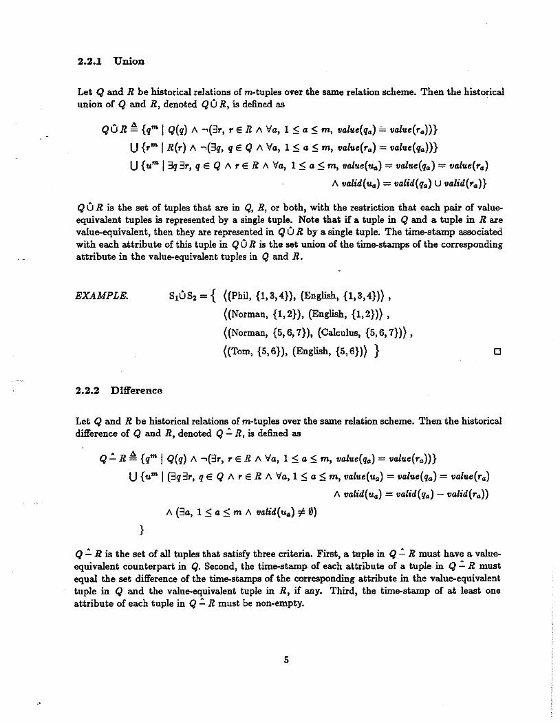
2.2.1 Union

Let q and R be historical relations of m-tuples over the same relation scheme. Then the historical union of q and R, denoted q 0 R, is defined as

qOR ~ {qm I CJ(q) /1. ~(3r, r E R /1. Va, 1:::; a:::; m, 11alue(q4 ) = 11alue(r4 ))}

U {rm I R(r) /1. -.(3q, q E CJ /1. Va, 1:::; a:::; m, 11alue(r4 ) = 11alue(q4 ))}

U { um l3q 3r, q E q /1. r E R /1. Va, 1 5 a 5 m, 11alue(u4 ) = 11alue(q4 ) = 11alue(r4 )

/1. 11alid(u4 ) = 11alid(q4 ) U 11alid(r4 )}

q 0 R is the set of tuples that are in Q, R, or both, with the restriction that each pair of value­equivalent tuples is represented by a single tuple. Note that if a tuple in q and a tuple in R are value-equivalent, then they are represented in q 0 R by a single tuple. The time-stamp associated with each attribute of this tuple in q 0 R is the set union of the time-stamps of the corresponding attribute in the value-equivalent tuples in q and R.

EXAMPLE.

2.2.2 Difference

s10S2 = { ((Phil, {1,3,4}), (English, {1,3,4})},

((Norman, {1,2}), (English, {1,2})},

((Norman, {5,6, 7}), (Calculus, {5,6, 7})},

((Tom, {5,6}), (English, {5,6})} } 0

Let q and R be historical relations of m-tuples over the same relation scheme. Then the historical difference of q and R, denoted q .:. R, is defined as

q.:. R ~ {qm I CJ(q) /1. ~(3r, r E R II Va, 1 :::; a 5 m, 11alue(q4 ) = 11alue(r4 ))}

U {um I (3q3r, q E q /1. r E R /1. Va, 1 5 a :5 m, 11alue(u4 ) = 11alue(q4 ) = 11alue(r4 )

/1. 11alid(u4 ) = 11alid(q4 )- llalid(ra))

/1. (3a, 1 :5 a :5 m /1. 11alid( u4 ) # 0)

}

q .:. R is the set of all tuples that satisfy three criteria. First, a tuple in q .:. R must have a value­equivalent counterpart in q. Second, the time-stamp of each attribute of a tuple in q.:. R must equal the set difference of the time-stamps of the corresponding attribute in the value-equivalent tuple in q and the value-equivalent tuple in R, if any. Third, the time-stamp of at least one attribute of each tuple in q .:. R must be non-empty.

5

.•

EXAMPLE. St.: S2 = { ((Phil, {1}), (English, {1})} ,

((Norman, {1,2}), (English, {1,2})) ,

((Norman, {5,6}), (Calculus, {5,6})} } D

· 2.2.3 Cartesian Product

Let Q be an historical relation of mt·tuples and R be an historical relation of m2-tuples. Then Q X R, the historical cartesian product of Q and R, is defined as

QxR~ {u"'•+m•l (3q, q E Q II 'Ia, 1 ~a :5 mt, ualue(ua) = ualue(qa) II ualid(ua) = ualid(qa))

II (3r, r E R II 'Ia, 1 ~a~ m2, ualue(um,+a) = ualue(ra) II ualid(Um,+a) = ualid(ra))

}

The cartesian product operator for historical relations is identical to the cartesian product operator for snapshot relations. Q x R is the set of (mt + m2)-tuples whose components u1, ... , Um, form a tuple in Q and whose components ""'•+1> ... , Um1+mo form a tuple in R.

EXAMPLE.

S1x S3 = { ((Phil, {1,3,4}), (English, {1,3,4}), (Phil, {1,2,3}), (Kansas, {1,2,3})},

((Phil, {1,3,4}), (English, {1,3,4}), (Phil, {4,5,6}), (Virginia, {4,5,6})},

((Phil, {1,3,4}), (English, {1,3,4}), (Norman, {1,2,5,6}), (Virginia, {1,2,5,6})},

((Phil, {1,3,4}), (English, {1,3,4}), (Norman, {7,8}), (Texas, {7,8})},

((Norman, {1,2}), (English, {1,2}), (Phil, {1,2,3}), (Kansas, {1,2,3})},

((Norman, {1,2}), (English, {1,2}), (Phil, {4,5,6}), (Virginia, {4,5,6})},

((Norman, {1,2}), (English, {1,2}), (Norman, {1,2,5,6}), (Virginia, {1,2,5,6})},

{(Norman, {1,2}), (English, {1,2}), (Norman, {7,8}), (Texas, {7,8})),

((Norman, {5,6}), (Calculus, {5,6}), (Phil, {1,2,3}), (Kansas, {1,2,3})},

((Norman, {5,6}), (Calculus, {5,6}), (Phil, {4,5,6}), (Virginia, {4,5,6})},

((Norman, {5,6}), (Calculus, {5,6}), (Norman, {1,2,5,6}), (Virginia, {1,2,5,6})},

((Norman, {5,6}), (Calculus, {5,6}), (Norman, {7,8}), (Texas, {7,8})) }

Let this be relation S4 over the relation scheme {SName, Course, HName, State}. D

6

,•

2.2.4 Selection

Let R be an historical relation of m-tuples. Also, let F be a boolean function involving

• Attribute names N1, ... , N.,.;

• Constants from the domains Dr. ... , /).,.;

• Relational operators <, =, >;and

• Logical operators 11, V, and ~

where, to evaluate F for a tuple r, r E R, we substitute the value components of the attributes of r for all occurrences of their corresponding attribute names in F. Then the historical selection of R, denoted by iTF(R), is defined as

iTF(R) A {r"' I r E R 1\ F( va/ue(ri), ... , va/ue(r.,.))}

Thus, u is identical to IT in the snapshot algebra. iTF(R) is simply the set of tuples in R for which F is true.

EXAMPLE.

USNamo=HName(S4) =

{ ((Phil, {1,3,4}), (English, {1,3,4}), {Phil, {1,2,3}), (Kansas, {1,2,3})),

((Phil, {1,3,4}), (English, {1,3,4}), (Phil, {4,5,6}), (Virginia, {4,5,6})),

((Norman, {1,2}), (English, {1,2}), (Norman, {1,2,5,6}), (Virginia, {1,2,5,6})),

((Norman, {1,2}), (English, {1,2}), (Norman, {7,8}), (Texas, {7,8})),

((Norman, {5,6}), {Calculus, {5,6}), (Norman, {1,2,5,6}), (Virginia, {1,2,5,6})),

((Norman, {5,6}), (Calculus, {5,6}), (Norman, {7,8}), (Texas, {7,8})) }

Let this be relation S5 over the relation scheme {SName, Course, HName, State}. D

2.2.5 Projection

Let R be an historical relation of m-tuples and let a1, ... , a,. be distinct integers in the range 1 tom. Then the historical projection of R, denoted by ifN.,, ... , N •• (R), is defined as

7

..

iN.1

, ••• ,Non (R) ~ { un J {Ill, 1 ~ 1-s; n, Vt, t E valid(u1),

3r,(rER

}

)

II Vh, 1 -s; h ~ n, value(u~o) = value(r.,)

II t E valid(r.,))

II (Vr, (r E R II VI, 1 ~I~ n, value(r01 ) = value(u,)),

Vh, 1 -s; h -s; n, valid(r.,) ~ valid(u~o)

)

II (31, 1 ~I~ n II valid(ul) # 0)

Like the projection operator for snapshot relation, the projection operator for historical relations retains, for each tuple, only the tuple components that correspond to the attribute names in {N • ., ... , N.n}. All other tuple components are removed. Value-equivalent tuples in the resulting set are then combined and tuples that have an empty valid component for all tuple components are removed.

EXAMPLE. isN.,..,state(Ss) = { ((Phil, {1,3,4}), (Kansas, {1,2,3})),

{(Phil, {1,3,4}), (Virginia, {4,5,6})),

{(Norman, {1,2,5,6}), (Virginia, {1,2,5,6})),

{(Norman, {1,2,5,6}), (Texas, {7,8})) }

Let this be relation Se over the relation scheme EnroUment = {Name, State}. Also assume that in this relation the time-stamp associated with the value of the attribute Name represents the interval(s) when the specified student was enrolled and that the time-stamp associated with the value of the attribute State represents the interva!(s) when the student was a resident of the specified state. 0

The operator i also supports projections on expressions. For an arbitrary n, let Evalue~, 1 -s; I -s; n, be an arbitrary expression involving the attribute names N., 1 -s; a -s; m. Evalue1 is evaluated, for a tuple r, r E R, by substituting the value components of the attributes of r for all occurrences of their corresponding attribute names in Evalue,. Also, let Evalid~, 1 ~ I -s; n, be an arbitrary expression involving the attribute names N., 1 -s; a -s; m, where Evalid1 is evaluated for a tuple r, r E R, by substituting the valid components of the attributes of r for all occurrences of their corresponding attribute names in Evalid,. In addition, assume that evaluation of Evalue1 for every tuple r produces an element of the domain Db, 1 -s; b -s; m, and that evaluation of Evalid1 produces an element of the domain ~(T). Then the definition of i, now denoted by i(Evalue1 , Evalidt), ... , (Evolu<n, Evalid.) (R), is constructed from the definition above simply by substituting Evalue~o(r) for value(r.,), Evalid~o(r) for valid(r.,), Evalue1(r) for value(r • .), and Evalid,(r) for valid(r.1). Note that this definition of the i operator is simply a more general

8

..

version of the definition presented earlier, where N.,, 1 ~ l ~ n, is assumed to be the ordered pair of expressions (N.,, N.,).

2.2.6 Historical Derivation

The historical derivation operator 6 is a new operator that does not have an analogous snapshot operator. It replaces the time-stamp of each attribute in a tuple with a new time-stamp, where the new time-stamps are computed from the existing time-stamps of the tuple's attributes. 6 is effectively a combination of selection and projection on a tuple's attribute time-stamps.

Several functions, defined on the domains T and ~(T), are used either directly or indirectly in the definition of the historical derivation operator. Before defining the derivation operator itself, we describe informally these auxiliary functions. Formal definitions appear in Appendix B.

FIRST takes a set of times from the domain ~(T) and maps it into the earliest time in the set.

LAST takes a set of times from the domain ~(T) and maps it into the latest time in the set.

PRED is the predecessor function on the domain T. It maps a time into its immediate predecessor in the linear ordering of all times.

SUCC is the successor function on the domain T. It maps a time into its immediate successor in the linear ordering of all times.

EXTEND maps two times into the set of times that represents the interval between the first time and the second time.

INTERVAL maps a set of times into the set of intervals containing the minimum number of non-disjoint intervals represented by the input set. Each time in the input set appears in exactly one interval in the output set and each interval in the output set is itself represented by a set of times.

EXAMPLE. Consider the following tuple taken from the relation S6 defined previously:

then

r= ((Norman, {1,2,5,6}), (Texas, {7,8})}

INTERVAL(valid(r(Name))) = { {1, 2}, {5, 6}}

INTERVAL(valid(r(State))) = {{7, 8}} 0

Given these auxiliary functions, we can now define the historical derivation operator on his­torical relations. Let R be an historical relation of m-tuples. Let v., 1 ~ a ~ m, be temporal functions involving

9

.•

• Attribute names N1, ... , Nm;

• Constants from the domain I of non-disjoint intervals defined in Appendix B;

• Functions FffiST, LAST, and EXTEND; and

• Set operators u, n, and -;

and let G be a boolean function involving

• Temporal functions, as just described;

• Relational operators <, =,and >; and

• Logical operators A, V, and ~.

The functions G and V.,, 1 :s; a :s; m, are always evaluated for a specific assignment of non­disjoint intervals to attribute names N1. ... , Nm. G evaluates to either true or false and v. evaluates to an element of ~(T). For a tuple r, r E R, and intervals IN., 1 :s; c :s; m, IN. E INTERVAL( valid(r.)), we evaluate G(IN., ... , IN.) by substituting IN. for all occurrences of Nc in G. Likewise, we evaluate V.(IN., ... , IN.) by substituting IN. for all occurrences of N. in v.. H any one of r's attribute values has a disjoint tinle-stamp, there will be multiple distinct evaluations of G (and V.,) for r, one for each possible assignment of intervals to attribute names, each resulting in a value of true or false for G (and a set of tinle quanta for V.,).

We can now define the derivation of the historical relation R, denoted 6a, v,, ... , v. (R), as

6a, v1 , .•. , Vm (R) ~ {um l3r, (r E R

II Va, 1 :s; a :s; m,

(value( u.,) = value( r .,)

II (Vt, t E valid(u.,),

)

3IN1 • •• 3IN., (IN, E INTERVAL(valid(r1)) A .. ·

II IN. E INTERVAL( valid(rm))

A G(IN., ... , IN.)

II t E V0 (IN., ... , INm)

)

A (VIN, ... VIN., (IN, E INTERVAL(validh)) II .. ·

II INm E INTERVAL(valid(rm))

II G(IN., ... , INm)),

V.(IN., ... , INm) ~ valid(u.)

10

.•

)) 1\ 3a, 1.::; a.::; m 1\ valid(u.) =f. 0

)}

For a tuple r, r E R, the historical derivation operator determines new time-stamps for r's at­tributes. The historical derivation function first determines all possible assignments of intervals to attribute names for which the boolean function G is true. For each assignment of intervals to attribute names for which G is true, the operator evaluates v., 1 .::; a .::; m. The sets of times resulting from the evaluations of v. are then combined to form a new time-stamp for attribute N •. For notational convenience, we assume that if only one V-function is provided, it applies to all attributes.

EXAMPLES.

D(NamenStat•)=Name,Name(Ss) = { {(Phil, {1}), (Kansas,{1})},

{(Norman, {1,2,5,6}), (Virginia, {1,2,5,6})),}

In this example, G is (Name 0 State) = Name and V1 and V2 are both Name. A student tu­ple s, s E Sa, satisfies condition G if the student had at least one interval of enrollment (i.e., IName E INTERVAL(valid(s(Name)))) during which his home state (i.e, State) did not change (i.e., (INamenlstate) =I Name, where lstat• E INTERVAL(valid(s(State)))). The new time-stamp for each attribute of a tuple that satisfies G for some assignment of intervals lName and lstat• is simply the union of the lName intervals from each assignment of intervals that satisfy G. In the first tuple in Ss, there are three intervals, two assigned to the attribute Name ({1}, {3,4}) and one assigned to the attribute State ({1,2,3}). From this tuple, we find that Phil was a resident of

Kansas during his first interval of enrollment (G({1}, {1,2,3}) = {1} n {1,2,3} '!:. {1}) but was a resident of Kansas during only part of his second interval of enrollment (G({3,4}, {1,2,3}) = {3, 4}n{1,2,3} =f. {3,4}). Hence, this tuple's attributes are assigned a time-stamp of {1} in there­sulting relation. From the second tuple in Ss we find that Phil was not a resident of Virginia during his first interval of enrollment (G({1}, {4, 5, 6}) = {1} n {4, 5,6} =f. {1}) and lived in Virginia dur­ing only part of his second interval of enrollment (G({3,4}, {4,5,6}) = {3,4} n {4, 5,6} =f. {3,4}). Hence, the time-stamp for this tuple's attributes would be assigned the empty set in the result­ing relation except the definition of the historical derivation operator disallows tuples whose at­tributes all have an empty time-stamp. This tuple is therefore eliminated and does not appear in the resulting relation. From the third tuple in Ss we find that Norman was a resident of Vir-

ginia during both of his intervals of enrollment (G({1,2}, {1,2}) = {1,2} n {1,2} '!:. {1,2} and

G({5, 6}, {5, 6}) = {5,6}n{5, 6} '!:. {5, 6} ). Hence, this tuple's attributes are assigned a time-stamp of {1, 2, 5, 6} in the resulting relation. From the fourth tuple in Ss we find that Norman was not a resident of Texas at any time during his enrollment (G({1,2}, {7,8}) = {1,2}n{7,8} =f. {1,2} and G({5,6}, {7,8}) = {5,6} n{7,8} =f. {5,6}); this tuple is therefore eliminated from the resulting relation.

11

6(No,..nStote);>!N..,.ei\(No,..nStote);t0,NomenStote{Sa) = { ({Phil, {3}), {Kansas, {3})),

({Phil, {4}), {Virginia, {4})) }

A student tuples, s E Sa, satisfies condition G if the student had at least one interval of enrollment during which his home state changed. The new time-stamp for each tuple that satisfies G for some assignment of intervals lN4 ,.. and lstote is the union of I Nom• n lstote from each assignment of intervals that satisfy G. From the first tuple in S6 we find that Phil had one interval of enrollment

. ~ ~ during which his home state changed (i.e., {3,4} n {1,2,3} f. {3,4} and {3,4} n {1,2,3} f. 0). Hence, this tuple's attributes are assigned a time-stamp of {3,4} n {1,2,3} = {3} in the resulting relation. From the second tuple in Sa we find that Phil had one interval of enrollment during which his home state changed. Hence, this tuple's attributes are assigned a time-stamp of { 4} in the resulting relation. Note that Norman does not satisfy the restriction; his home state was the same during his two periods of enrollment. Hence, the third and fourth tuples are eliminated from the resulting relation. D

Note that the historical derivation operator actually performs two functions. First, it performs a selection function on the valid component of a tuple's attributes. For a tuple r, if G is false when an interval from the valid component of each of r's attributes is substituted for each occurrence of its corresponding attribute name in G, then the temporal information represented by that combination of intervals is not used in the calculation of the new time-stamps for r's attributes. Secondly, the derivation operator calculates a new time-stamp for attribute N4 , 1 ::;; a ::;; m, from those combinations of intervals for which G is true, using V4 • If Vt, . '., Vm are all the same function, the tuple is effectively converted from attribute time-stamping to tuple time-stamping.

The derivation operator is necessarily complex because we allow set-valued time-stamps; it would have been less complex if we had disallowed set-valued time-stamps. Then the derivation operator could have been replaced by two simpler operators, analogous to the selection and projec­tion operators, that would have performed tuple selection and attribute projection in terms of the valid components, rather than the value components, of attributes. But, as we will see in Section 4, disallowing set-valued time-stamps would have required that the algebra support value-equivalent tuples, which would have prevented the algebra from having several other, more highly desirable properties.

2.3 Aggregates

Aggregates allow users to summarize information· contained in a relation. Aggregates are catego­rized as either scalar aggregates or aggregate functions. Scalar aggregates return a single scalar value that is the result of applying the aggregate to a specified attribute of a snapshot relation. Aggregate functions, however, return a set of scalar values, each value the result of applying the aggregate to a specified attribute of those tuples in a snapshot relation having the same values for certain attributes. Database management systems based on the relational model typically provide several aggregate operators. For example, Ingres [Stonebraker et a!. 1976] provides a count, sum,

12

,•

average, minimum, maximum, and any aggregate operator. Ingres also provides two versions of the count, sum, and average operators, one that aggregates over all values of an attribute and one that aggregates over only the unique values of an attribute.

Several researchers have investigated aggregates in time-oriented relational databases [Ben­Zvi 1982, Jones eta!. 1979, Navathe & Ahmed 1986, Snodgrass, eta!. 1987, Tansel, et al. 1985]. Their work reflects the consensus that aggregates when applied to historical relations should return not a scalar value, but a distribution of scalar values over time. Jones, et a!. also introduced the concepts of instantaneous aggregates and cumulative aggregates. Instantaneous aggregates return, for each time t, a value computed only from the tuples valid at time t. Cumulative aggregates return, for each time t, a value computed from all tuples valid at any time up to and including t, regardless of whether the tuples are still valid at time t. Note that a time t has meaning only when defined in terms of the time granularity. Hence, instantaneous aggregates can be viewed as aggregates over an interval whose duration is determined by the granularity of the measure of time being used. Others have generalized the definition of instantaneous and cumulative aggregates by introducing the concept of moving aggregation windows [Navathe & Ahmed 1986]. For an aggregation window function w from the domain T into the non-negative integers, an aggregate returns, for each time t, a value computed from tuples valid either at time t or at some time in the interval of length w(t) immediately preceding time t. Hence, an instantaneous aggregate is an aggregate with an aggregation window function w(t) = 0 and a cumulative aggregate is an aggregate with an aggregation window function w(t) = oo.

Klug introduced an approach to handle aggregates in the snapshot algebra [Klug 1982]. His approach makes it possible to define aggregates in a rigorous way. We use his approach to define two historical aggregate functions for our algebra:

• A, that calculates non-unique aggregates, and -• AU, that calculates unique aggregates.

These two historical aggregate functions serve as the historical counterpart of both scalar aggregates and aggregate functions.

The historical aggregate functions must contend with a variety of demands that surface as parameters (subscripts) to the functions. First, a specific aggregate (e.g., count) must be specified. Secondly, the attribute over which the aggregate is to be applied must be stated and the aggregation window function must be indicated. Finally, to accommodate partitioning, where the aggregate is applied to partitions of a relation, a set of partitioning attributes must be given. These demands complicate the definitions of A and Au, but at the same time ensure some degree of generality to these operators.

For both definitions, let R be an historical relation of m-tuples over the relation scheme NR = {Nb ... , N,.}. Also let a, c1, ... , c,. be distinct integers in the range 1 tom and Q be an historical relation over the relation scheme Nq, with the restrictions that Nq ~ NR and {Na, N • ., ... , N •• } ~ Nq. Finally, let X= {N • ., ... , N •• }. If X is empty, our historical aggregate functions simply calculate a single distribution of scalar values over time for an arbitrary aggregate applied to attribute Na of relation R. If X is not empty, our historical aggregate functions calculate, for

13

,•

each subtuple in Q formed from the attributes X, a distribution of scalar values over time for an arbitrary aggregate applied to attribute N ~ of the subset of tuples in R whose values for attributes X match the values for attributes X of the tuple in Q. Hence, X corresponds to the by-list of an aggregate function in conventional database query languages. Assume, as does Klug, that for each aggregate operation (e.g., count) we have a family of scalar aggregates that performs the indicated aggregation on R (e.g., COUNTN, COUNTN., ••• , COUNTN. where COUNTN., 1 :5 a :5 m, counts the (possibly duplicate) values of attribute N4 of R). We will define our historical aggregate functions in terms of these scalar aggregates.

2.3.1 Partitioning Function

Before defining the historical aggregate functions A and AU, we define a partitioning function that will be used in their definitions.

a PARTITION(R, q, t, w, N~, X)=

{um I (3r), (r E R 1\ Ill, 1:51:5 n, tlalue(rc1) = tlalue(q.,)

1\ lfd, 1 :5 d :5 m, tlalue(ud) = t1a/ue(r4)

1\ lfd, 1 :5 d :5 m,

((1ft', t' E t~alid(ud),

)

3Id, (IdE INTERVAL(t~alid(r4))

)

1\ t- w(t) < 1--+ (I4 n EXTEND(!, t) #- 0)

1\ t- w(t) ~ 1--+ (Id n EXTEND(t- w(t), t) #- 0)

1\ t1 E !4

1\ (lfld, (IdE INTERVAL(t~alid(rd))

))

1\ t- w(t) < 1--+ (Id n EXTEND(!, t) #- 0)

1\ t- w(t) ~ 1--+ (Id n EXTEND(t- w(t), t) #- 0))

!4 ~ tlalid(u.)

1\ t1a/id( u~) #- 0

1\ VI, 1 :5 I :5 n, 11alid(u.,) #- 0

)}

where q E Q, t E T, w is an aggregation window function, and 1 :5 a :5 m. This function retrieves from R those tuples that have the same value component for attribute N., 1 :5 I :5 n, as q and

14

have time t or some time in the interval of length w(t) immediately preceding tin the time-stamp of attributes N4 , N • ., .. . , and N ••. Note that the time-stamp of attribute Na, 1 :5 d :5 m, in the resulting relation is constructed from those intervals in the time-stamp of attribute Na in R that contain timet or some time in the interval of length w(t) immediately preceding t. The predicates t- w(t) < 1 -+ • • • and t-w(t) 2:: 1 -+ • • • are used here to ensure that PARTITION is well-defined as EXTEND is defined only for elements in the domain T.

EXAMPLES.

PARTITION(Se, ( ), 5, O, Name, 0)= { ((Norman, {5,6}), (Virginia, {5,6}))

((Norman, {5, 6}), (Texas, 0)} }

Because time 5 is specified and the aggregation window function, denoted by zero, is the constant function w(t) = 0, tuples are selected whose time-stamp for attribute Name overlaps time 5. Only the third and fourth tuples in Ss satisfy this requirement. The partitioning function here effectively returns the tuples for those students who were enrolled in school at time 5. Note that the time-stamp of each attribute in the selected tuples has been restricted to the interval from the attribute's original time-stamp overlapping time 5, if any.

PARTITION(Ss, ((Phil, {1,3,4}), (Virginia, {4,5,6})), 5, 0, Name, {State})=

{ ((Norman, {5,6}), (Virginia, {5,6})} }

where Q is here assumed to be S6 • Tuples are selected for those students who were enrolled in school and a resident of Phil's state (Virginia) at time 5. Only the third tuple in Ss satisfies this requirement. Although Phil was a resident of Virginia at time 5, he was not enrolled in school at time 5. Hence, the second tuple in Ss is not included in this partition.

PARTITION(Ss, ((Phil, {1,3,4}), (Virginia, {4,5,6})), 5, 1, Name, {State})=

{ ((Phil, {3,4}), (Virginia, {4,5,6})}

((Norman, {5,6}), (Virginia, {5,6})} }

Here tuples are selected for those students who were enrolled in school and a resident of Virginia within a year (w(t) = 1) oftime 5. Both the second and third tuples in Se satisfy this requirement. The second tuple in Ss is now included in the partition because Phil was a resident of Virginia and enrolled in school at time 4. 0 ·

2.3.2 Non-unique Aggregates

The historical aggregate function A calculates, for each tuple in Q, a distribution of scalar values over time for an arbitrary aggregate applied to attribute N 4 of the subset of tuples in R whose

15

..

value component for attribute Nc., 1 $ l $ n, matches the value component for attribute Nc1 of the tuple in Q. If X is empty, A simply calculates a single distribution of scalar values over time for the aggregate applied to attribute N4 of R. If we let I represent an arbitrary family of scalar aggregates and w represent an aggregation window function, then we can define A on the historical relations Q and R, denoted by AJ,w,N.,x(Q, R), as

Af,..,,N.,x(Q, R) ~

Ov,, ter(1fxu{N.,.} ({q II (y, {t}) I q E Q

At- w(t) < 1-+ (1lalid(q4 ) nEXTEND(1, t) # 0

A Y l, 1 $ l $ n,

1lalid(q.,) nEXTEND(l, t) # 0)

At- w(t) ;?; 1-+ ( valid(q4 ) n EXTEND(t- w(t), t) # 0

II Yl, 1$1$ n,

1Jalid(q.1) nEXTEND(t- w(t), t) # 0)

A y = IN.(q, t, PARTITION(R, q, t, w, N4 , X))

}))

where "II" denotes concatenation and N499 is the attribute name assigned the aggregate value (y, {t}). If X is not empty, function A first associates with each timet the partition of relation Q whose tuples have t, or a time in the interval of length w(t) immediately preceding t, in the valid component of attributes N4 , N.,, .. . , and Nc.· For each of these partitions, A then constructs a set of historical tuples. Each tuple in the set contains all the attributes X of a tuple q in the partition and a new attribute. This new attribute's valid component is the time t corresponding to the partition and its value component is the scalar value returned by the aggregate IN., when IN. is applied to the partition of R whose tuples have value components that match q's value components for attributes X and whose valid components for attributes N4 , Nc,, ... , and N •• overlap either t or the interval of length w(t) immediately preceding t. Then A performs an historical union of the resulting sets of historical tuples to produce a distribution of aggregate values over time for each tuple in Q. If X is empty, A constructs for each time t an historical relation that is either empty or contains a single tuple. If the valid component of attribute N4 of no tuple r in R overlaps t or the interval of length w(t) immediately preceding t, then the historical relation is empty. Otherwise, the historical relation contains a single tuple whose valid component is the time t and whose value component is the scalar value returned by the aggregate IN., when IN. is applied to the partition of R whose tuples have a valid component for attribute N4 that overlaps either tor the interval of length w( t) immediately preceding t. Then A performs an historical union of the resulting sets of historical tuples to produce a single distribution of aggregate values over time.

Note that a tuple and a time are passed as parameters to the scalar aggregate IN., along with a partition of R, in the definition of A. Although most aggregate operators can be defined in terms of a single parameter, the partition of R, the additional parameters are present because aggregates that evaluate to events or intervals, one of which is defined in Section 3.3, require them.

16

.•

EXAMPLES. AcoUNT,o,state,0(*state(Ss), Ss) = { ((1, {3,4,7,8})},

((2, {1,2,5,6})) }

The function A computes the number of states in which enrolled students resided. Because w(t) = 0 and the time granularity of Se is a semester, the resulting relation represents aggregation by semester. Hence, the aggregate is in effect an instantaneous aggregate. For the interval {1, 2}, there were two states (Kansas in the first tuple and Virginia in the third tuple). For the interval {3,4}, there was one state (Kansas in the first tuple at time 3 and Virginia in the second tuple at time 4). For the interval {5,6}, there also was only one state (Virginia), but it appeared in both the second and third tuples. It was counted twice because the scalar aggregates embedded within A aggregate over duplicate values. For the interval {7,8}, there was only one state (Texas in the fourth tuple).

AcoUNT,l, State, 0(*state(Sa), Ss) = { ((1, {8, 9})),

((2, {1,2,3,4,5,6}))'

((3, {7})) }

Again, A computes the number of states in which enrolled students resided, but now w(t) = 1. Hence, the resulting relation now represents aggregation by year (assuming two semesters per year). Although nine does not appear in the time-stamp of attribute State in any tuple in Se, a count of one is recorded at time 9 because a tuple, the fourth tuple in Se, falls into the aggregation window at time 9.

AcoUNT,oo,State,0(,rstate(Ss), Ss) = { ((2, {1,2,3})),

((3, {4,5,6}))'

((4, {7,8, ... })) }

Now, with w(t) = oo, A computes a cumulative aggregate of the number of states in which enrolled students resided.

AcoUNT,O,Name,{State}(Ss, Ss) = { ((Kansas, {1,2,3}), (1, {1,2,3}))

((Virginia, {1,2,4,5,6}), (1, {1,2,4}))

{(Virginia, {1,2,4,5,6}), (2, {5,6}))

((Texas, {7,8}), (1, {7,8})) }

Here, A computes the instantaneous aggregate of the number of enrolled students who resided in each state. In effect, the aggregate is computed for each subset of tuples in Ss having the same value for the attribute State. For example, the first tuple is computed by selecting all the tuples in S6 with a state of Kansas and then performing the aggregate on this (smaller) set. 0

17

..

2.3.3 Unique Aggregates

The function A allows its embedded scalar aggregates to aggregate over duplicate attribute values. We now define an historical aggregate function Ali, identical to A with one exception; it restricts its embedded scalar aggregates to aggregation over unique attribute values. We define Ali on the historical relations Q and R, denoted by Ali/,.,, N., x( Q, R), as

- " AU1,w,N.,x(Q, R) =

Uvt,IET(irxu{N • .,} ({q II (y, {t}) I q E Q

1\ t- w(t) < 1-+ ( valid(qa) n EXTEND(!, t) # 0

1\ V 1, 1 ~ 1 ~ n,

valid(q,1) n EXTEND(!, t) # 0)

1\ t- w(t) ~ 1-+ (va1id(q4 ) nEXTEND(t- w(t), t) # 0

1\ V 1, 1 ~ 1 ~ n,

valid(q,,) nEXTEND(t- w(t), t) # 0)

1\ y = fN.(q, t, 5true,t(irN.(PARTITION(R, q, t, w, N 4 , X))))

}))

This definition differs from that of A only in that the historical projection on attribute N 4 of PARTITION( ... ) followed by the historical derivation eliminates duplicate values of the aggre­gated attribute before the scalar aggregation is preformed.

EXAMPLE. WcoUNT,O,Siate,0(irstate(Ss), Ss) = { ((1, {3,4,5,6,7,8})},

((2, {1,2})} }

This relation differs from the non-unique variant only during the interval {5,6}. Here, Virginia is correctly counted only once, even though there are two tuples valid during this interval with a state of Virginia. 0

2.3.4 Expressions in Aggregates

The functions A and Ali allow expressions to be aggregated and support aggregation by arbitrary expressions. Let Eaggregate be an arbitrary expression involving u historical aggregate functions. Also, assume that the v1" historical aggregate function applies the scalar aggregate /. to attribute Na, where the ag1regation window function is w., and the partitioning attributes are X •. Then the definition of A, now denoted by

18

is constructed from the definition of A above simply by substituting y = Eaggregate1 for y = !N.(- . . ). Eaggregate' is Eaggregate where each reference to the uth aggregate has been replaced by the expression fuN.,(q, t, PARTEION(R, q, t, w., Na., x.)). With these changes, A allows expressions to be aggregated. AU can be modified similarly.

If A and AiJ are to support aggregation by arbitrary expressions, changes must be made to the definitions of PARTITION, A, and Ail given above. First, let Eualue,, 1 ~ I ~ o, be an expression involving the attribute names Nc., ... , Nc •. Eualue1 is evaluated for a tuple r, r E R, by substituting the value components of the attributes of r for all occurrences of their corresponding attribute names in Eualue,. Secondly, let X = {Eualue1, ... , Eualue0 } and dt, ... , dp be the distinct integers in the range 1 to m sucli that Nd,, 1 ~ h ~ p, appears in at least one Eualue1, 1 ~I~ o. Then new definitions of PARTITION, A, and AiJ are constructed from the definitions above simply by substituting the predicate 'VI, 1 ~ I~ o, Eualue,(r) = Eualue1(q) for the predicate VI, 1 ~I~ n, value(rc1) = ualue(q.,) and the predicate VI, 1 ~I~ p, ualid(ud,) =j:. 0 for the predicate VI, 1 ~I~ n, ualid(u.,) =j:. 0 in the definition of PARTITION and substituting p for nand valid(%) for valid(qc1) in the definitions of A and Ail. With these changes, A and AiJ support aggregation by arbitrary expressions.

2.4 Preservation of the Value-equivalence Property

Theorem 1 The operators 0, :.., x, fr, i, o, A, and AiJ all preserue the value-equiualence property of historical relations.

PROOF. For the operators 0, :.., x, fr, and owe show that the contrapositive of the theorem holds, that is, if there are value-equivalent tuples in an operator's output relation, then there are value-equivalent tuples in at least one of its input relations. For the operators i, A, and Ail, we show by contradiction that there cannot be value-equivalent tuples in their output relations.

Case 1. 0. Assume that Q 0 R contains at least two value-equivalent tuples. From the definition of 0, each tuple in Q 0 R has a value-equivalent tuple in Q, R, or both. If two value-equivalent tuples u1 and u2 in Q 0 R do not have a value-equivalent tuple in R, then both are tuples in Q. Similarly, if they do not have a value-equivalent tuple in Q, then both are tuples in R. If they have a value-equivalent tuple in both Q and R, then each was constructed from a value-equivalent tuple in Q and a value-equivalent tuple in R. If both u1 and u2 had been constructed from the same tuple in Q and the same tuple in R, then u1 and u2 would be, by definition, the same tuple. Hence, they were constructed from different value-equivalent tuples in Q, R, or both.

Case £. :.. . Assume that Q :.. R contains at least two value-equivalent tuples. From the definition of:.., each tuple in Q:.. R has a value-equivalent tuple in Q but not in R or a value-equivalent tuple in both Q and R. If two value-equivalent tuples u1 and u2 in Q :.. R do not have a value-equivalent tuple in R, then both are tuples in Q. If they have a value-equivalent tuple in both Q and R, then each was constructed from a value-equivalent tuple in Q and a value-equivalent tuple in R. If both u1 and u2 had been constructed from the same tuple in Q and the same tuple in R, then u1 and u2 would be, by definition, the same tuple. Hence, they were constructed from different value-equivalent tuples in Q, R, or both.

19

..

Case 9. X. Assume that Q X R contains at least two value-equivalent tuples. From the definition of X, each tuple in Q X R is constructed from a tuple in Q and a tuple in R. If two value-equivalent tuples u1 and u2 in Q X R had been constructed from the same tuple in Q and the same tuple in R, then u1 and u2 would be, by definition, the same tuple. Hence, they were constructed from different value-equivalent tuples in Q, R, or both.

Case .4. u. Assume that up(R) contains at least two value-equivalent tuples. From the definition of u, each tuple in up(R) is a tuple in R. Hence, any two value-equivalent tuples in up(R) are also tuples in R.

Case 5. ii". Assume that ii"N.,, ... , N • .(R) contains at least two value-equivalent tuples. For any two such tuples there will be at least one time that appears in the time-stamp of an attribute of one tuple but not the other tuple; otherwise, they would be identical. Hence, let u1 and u2 be two value-equivalent tuples in ii"N.,, ... , N.A (R) such that there is a timet in the time-stamp of attribute Na., 1 ~ l ~ n, of u1 but not u2. From the first clause of the definition of ii", there is a tuple r, r E R, that has t in the time-stamp of attribute N41 and the same value for attributes N41 , ... , Na. as u1. But, from the second clause of the definition, the time-stamp of attribute N 41 of tuple r is a subset of the time-stamp of attribute N 41 of u2, as r also has the same value for attributes N41 , ••• , N4 A as u2. Hence, t is in the time-stamp of attribute Na, of u2, contradicting the assumption that tis in the time-stamp of attribute N 41 of u1 but not fl:. Similarly, we arrive at a contradiction if we assume that there is a time t in the time-stamp of attribute Na., 1 ~ l ~ n, of u2 but not u1. Hence, u1 and u2 have identical attribute time-stamps, which implies that they are the same tuple, contradicting the assumption that ii"N.,, ... ,N.A (R) contains at least two value­equivalent tuples. Note that the output relation of ii", unlike the output relations of 0, ..:, x, and u, would not contain value-equivalent tuples even if there were value-equivalent tuples in its input relation.

Case 6. 6. Assume that 6a, v, ... , vm(R) contains at least two value-equivalent tuples, u1 and u2. From the definition of 6, each tuple in 6a, v, ... , Vm (R) is constructed from one value-equivalent tuple in R. If u1 and u2 were constructed from the same value-equivalent tuple r, r E R, then they would be the same tuple, as 6 requires not only that every time t in the time-stamp of attribute Na, 1 ~ a~ m, of either u1 or u2 be in V4( ... ) and satisfy G( .. . ) for some assignment of intervals from the time-stamps of r's attributes to attribute names but that V4 ( •• • ) be a subset of the time-stamp of attribute N4 of both Ut and u2. Hence, u1 and u2 were constructed from different value-equivalent tuples in R.

Case 7. A. Assume that .A,,.,, N.,x(Q, R) contains at least two value-equivalent tuples. From Case 1 above, if .A,, w, N., x(Q, R) contains value-equivalent tuples, then the input relation to A's outermost 0 operator contains value-equivalent tuples. But, this relation is the output of ii", whose output relation was shown in Case 5 above never to contain value-equivalent tuples. Hence, our assumption that .A,, .. ,N.,x(Q, R) contains at least two value-equivalent tuples is contradicted.

Case 8. Au. Simply replace A with AU in Case 7. I

20

,•

2.5 Summary

We first introduced historical relations, in which attribute values are associated with set-valued time-stamps. We then defined eight historical operators:

• Five operators are analogous to the five standard snapshot operators: union (0), difference (.:),cartesian product (x), selection (<7), and projection (ii-).

• Historical derivation ( c5) effectively performs selection and projection on the valid-time dimen­. sion by replacing the time-stamp of each attribute of selected tuples with a new time-stamp.

• Aggregation (A) and unique aggregation (AU) serve to compute a distribution of single values over time for a collection of tuples.

We should mention several other operators that can exist harmoniously with these eight op­erators. Intersection (n), quotient (.f.), natural join (M), and 9-join (~) can all be defined in terms of the five basic operators, in an identical fashion to the definition of their snapshot coun­terparts. Finally, the historical rollback operator (p), defined elsewhere [McKenzie & Snodgrass 1987A], serves to generalize the algebra to handle temporal relations incorporating both valid and transaction time.

3 Equivalence with TQuel

We now show that the historical algebra defined above has the expressive power of the TQuel (Temporal QUEry Language) [Snodgrass 1987] facilities that support valid time. TQuel is a version of Que! [Held et al. 1975], the calculus-based query language for the Ingres relational database management system [Stonebraker et al. 1976], augmented to handle both valid time and transaction time. Two new syntactic and semantic constructs are provided to support valid time. The valid clause is the temporal analogue to Quel's target list; it is used to specify the value of the valid time for tuples in the derived relation. This clause consists of the keywords valid from to and two temporal expressions, each consisting of tuple variables, temporal constants, and the temporal constructors begin of, end of, overlap, and extend. The when clause is the temporal analogue to Que! 's where clause. This clause consists of the keyword when followed by a temporal predicate consisting of temporal expressions, the temporal predicate operators precede, overlap, and equal, and the logical operators or, and, and not. (Note that overlap is overloaded; it may be either a temporal constructor or a temporal predicate operator, with context differentiating the uses.) A third new construct, the as-of clause, is provided to handle transaction time but will not be considered here. We will generally limit our discussion of TQuel to its facilities for handling valid time.

Unlike our historical algebra, which assumes attribute time-stamping, TQuel assumes tuple time-stamping. The formal semantics of TQuel conceptually embeds its temporal relations in snapshot relations; such an embedding is done purely for convenience in developing the semantics. TQuel represents valid time by adding two time values to each tuple to specify the time when the

21

tuple became valid (i.e., From) and the time when the tuple became invalid (i.e., To). Also unlike our historical algebra, TQuel allows value-equivalent tuples in a relation but assumes that value­equivalent tuples are coalesced (i.e., tuples with identical values for the explicit attributes neither overlap nor are adjacent in time). AB we will see shortly, it is possible to convert the embedded, coalesced snapshot relations used in TQuel's formal semantics to historical relations.

3.1 TQuel Retrieve Statement

ABsume that we are given the k snapshot relations ~ •... , R~ whose schemes are respectively,

For notational convenience, we associate " 1 " with TQuel relations, tuple variables, and ex­

pressions to differentiate them from their counterparts in the historical algebra and assume that N1,1> ... , Nk,m• are unique. Furthermore, let it, i2, ... , i,. be integers, not necessarily distinct, in the range 1 to k and a1, 1 ~ l ~ n, be a distinct integer in the range 1 to m;1 • Then, the TQuel retrieve statement has the following syntax

range of r~ is .R~

range of r~ is R~

retrieve into R~+l (N.t;+l,l = r~1 .Nit, 41 • ••• , N~;+t,n = r~n·Nin,a,.)

valid from tJ to X

where .P when r

This statement computes a new relation R~+l over the relational scheme

Its tuple calculus statement has the following form

22

(1)

..

~+1 = { u"+2 I (3r\.)· · · (3r~)

(r{ E R{ 1\ • • • 1\ r~ E Rl,

1\ u(Nk+l, I)= ri, (N;1,a1 ) 1\ • • • 1\ u(Nk+l,n) = ,-:n (N;n,an)

1\ u(Fromk+l) = .P~((rHFrom1), rHTo1)), ... , (r~(Fromk), r~(Tok)))

1\ u(Tok+l) = .P~((rHFrom1), rHTo1)), ... , (r~(Fromk), t1,(Tok))) (2)

1\ Before(u(Fromk+l), u(Tok+l))

1\ .P~(rHN1,1), ... , r~(Nk,m1 ))

"r~((rHFromt), rHToi)), ... , (r~(Fromk), rHTok)))

)}

where Before is the "<" predicate on integers, the ordered pair (rl(From;), rl(To;)), 1::; i::; k, represents the interval fr:<From;), rl(To;)), and .P~, 'P'u, 'P'x, and r~ are the denotations described below of .p, v, x, and T respectively .

.P~ is obtained by replacing each occurrence of an attribute reference rl.N;, a. 1 ::; i ::; k, 1 ::; a :5 m;, in .p with rHN;,a) and each occurrence of a logical operator with its corresponding logical predicate. That is,

and~ 1\,

or-+ v, and

not --+ ..., •

.P~ and .P~ are obtained by replacing each occurrence of a tuple variable rl in v and X with the ordered pair (rl(From;), rl(To;)) and each occurrence of a temporal constructor with a corre­sponding function. That is,

,-: -+ (rl(From;), rl(To;))

begin of I -+ beginof(I),

end of I -+ endof(I),

I1 overlap I2 -+ o11erlap(Il> I2), and

h extend !, -+ eztend(I1, I2)

where beginof, endof, ot1erlap, and extend are functions on the domain I. Formal definitions for these functions are presented elsewhere [Snodgrass 1987].

r~ is obtained by replacing each occurrence of a logical operator in T with its corresponding logical predicate according to the rules given for its replacement in .p, replacing each occurrence of

23

..

a tuple variable or temporal constructor according to the rules given for their replacement in 11 and x, and replacing each occurrence of a temporal predicate operator with an analogous predicate on intervals. That is,

It precede I2 --> precede(lt, I2),

It overlap I2 --> overlap( It, I2), and

It equal I2 --> equal(It, I2)

where precede, overlap, and equal are predicates on the domain I. Formal definitions for these predicates are presented elsewhere [Snodgrass 1987].

3.2 Correspondence with the Historical Algebra

To compare the expressive power of TQuel and the historical algebra presented in Section 2, we first relate relations in the two systems, then expressions in the new TQuel clauses, and finally the retrieve statement with algebraic expressions.

Definition 1 The transformation function T maps a TQuel embedded snapshot relation over the scheme {Nt, ... , N,., From, To} into its equivalent historical relation, valid in our historical algebra over the scheme {Nt, ... , N,.}.

T(R') ~ {u"' I (\fa, 1::; a::; m, \ft, t E valid(u(Na)),

)

3r', (r' E R'

A \fc, 1 ::; c::; m, value(u(N.)) = r1(N.)

AtE EXTEND(r'(From), SUCC(r'( To)))

)

A ('v'r', (r' E R' A \fa, 1 ::; a::; m, r'(N.) = ualue(u(N.))),

\fc, 1::; c::; m, EXTEND(r'(From), SUCC(r'(To))) ~ valid(u(N.)))

)}

The first clause of this definition ensures that eaclt tuple in T(R') has at least one value-equivalent tuple in R. The second clause in the definition ensures that each subset of value-equivalent tuples in R is represented by a single tuple in T(R'). Note also that the same time-stamp is assigned to each attribute of a tuple in T(R'). This time-stamp is simply the union of the time-stamps of the tuple's value-equivalent tuples in R'. Because TQuel assumes that value-equivalent tuples are coalesced, the time-stamp of each tuple in R' is a distinguishable interval of time in the attribute time-stamps of its value-equivalent counterpart in T(R'), as shown by the following lemma.

24

..

Lemma 1 Vr, r E T(R'), 'Ia, 1 $a$ m, VI, I EINTERVAL(valid(r(N.))),

3r', (r' E R'

/\ Vc, 1::;; c::;; m, value(r(N.)) = r'(Nc)

/\I= EXTEND(r'(From), SUCC(r'(To)))

)

PROOF. Apply the definitions of coalescing and INTERVAL toT and simplify. I

Definition 2 We define a m+2-tuple TQuel relation R' and am-tuple relation R in our historical algebra to be equivalent if, and only if, R = T(R'). In addition, we define a TQuel query and an expression in our historical algebra. to be equivalent if, and only if, they evaluate to equivalent relations.

Let w.,, ~.,and ~x be the denotations in our algebra of t/r, v, and X respectively. w., is obtained by replacing each occurrence of rl(N;, 0 ), 1::;; i $ k, 1 $a$ m;, in VI~ with N;, •. ~u and ~X are obtained by replacing each occurrence of an ordered pair (rl(From;), rl(To;)), 1 $ i $ k, in~~ and ~~ with N;,1 and each occurrence of a TQuel function with its algebraic equivalent. That is,

(r;(From;), r;(To;)) -+ N;,1,

beginof(I) -+ FffiST(I),

endof(I) -+ LAST(!),

overlap(It. I2) -+ It n !2, and

eztend(I1, h) -+ EXTEND(FIRST(lt), LAST( h)).

Also let r, be the denotation in our algebra of r. r, is obtained by replacing each occurrence of an ordered pair (rl(From;), rl(To;)) and each occurrence of a TQuel function in r~ with its algebraic equivalent according to the rules above and each occurrence of the predicates precede, overlay, and equal with its algebraic equivalent. That is,

precede( it, I2) -+ LAST(ft) < FIRST(I2) V LAST(I1) = FffiST(I2),

overlap(ft, I2) -+ It n I2 # 0, and

equal( It, h) -+ It= I2.

Note from the definition of T( R') that a tuple in T( R') has the same time-stamp for each of its attributes. Hence, although we require that each occurrences of an ordered pair (rl(From;), rl( To;)) in~~' ~X' and r~ be replaced with the same attribute name (i.e., N;, 1), we could have specified any attribute of relation R;.

We will need the following two lemmas in the equivalence proof to be presented shortly.

25

Lemma 2 <Pv, <Px, and r r are semantically equivalent to <P~, <P~, and r~ respectively. That is, the result of evaluating <P~, <P~, and r~ for tuples rl, rl E .RJ, 1 :5 i :5 k, is the same as the result of evaluating <Pv, <Px, and r, for the intervals I;, I; = EXTEND(rl(From;), SUCC(rl(To;))) substituted for the attribute name Ni,l·

PROOF. The semantic equivalence follows directly from the definitions of the functions used in ~. <P~, and 'r~ [Snodgrass 1987]. I

Lemma 3 t E EXTEND(<P~( ... ), SUCC(<P'x(· .. ))) --+ Before(<P~( .. . ), <P'x(· . . )).

PROOF. It follows directly from the definition of EXTEND, given in Appendix B, that t E EXTEND(<P~( ... ), SUCC(<P~( ... ))) implies <P~( ... ) :5 t < <P~( ... )), which in turn implies Before(<P~( .. . ), <P~( ... )) I

Having defined the algebraic equivalents of TQuel relations and expressions in the new TQuel clauses, we can now define th·e algebraic equivalent of a TQuel retrieve statement. Every Que! retrieve statement (a target list and where clause) is equivalent to an algebraic expression that represents cartesian product of the relations associated with tuple variables, followed by selection by the where-clause pr~dicate, and then projection on the attributes in the target list. Similarly, every TQuel retrieve statement is equivalent to an algebraic expression that represents cartesian product of the referenced relations, followed by selection by the where-clause predicate, historical derivation as specified by the when and valid clauses, and then projection on the attributes in the target list.

Theorem 2 Every TQuel retrieve statement of the form of (1) found on page 22 is equivalent to an expression in our historical algebra of the form

R = 1l-N;1,.

1, ..• ,N;., • .(Or,,EXTEND(~ •• sucq~xll(ut~,.(T(RDx ... xT(R~)))). (3)

PROOF. To prove that Rand R~+l are temporally equivalent, we must show that R = T(R~+l). From set theory and the definition ofT, it follows that Rand T(R~+l) are equal if, and only if, the following holds.

('v'r, r E R, Va, 1 :5 a :5 n, Vt, t E valid(r(N.)),

3r~+l, ( r~+l E R~+l

A Vc, 1 :5 c :5 n, value(r(Nc)) = r~+l(Nk+l,c)

AtE EXTEND(r~+l(Fromk+l), SUCC(r~+l(Tok+l)))

)

)

26

(4)

..

Vc, 1 5 c 5 n,

EXTEND(r~+l(FromHt), SUCC(r~+1(To&+l))) ~ ualid(r(N.))

)

· To prove the validity of (4), we show that the tuple calculus for R reduces to (4). First, construct · the tuple calculus statement for R from the definitions of the historical operators x, & , S, and ;r,

using straightforward substitution, change of variable, and simplification (i.e., the definition of T(Rl_)x ... xT(R~) obtained from the x operator is substituted for references to the historical relation in the definition of & , etc.).

1 {r"l (Vc, 1 5 c 5 n, Vt, t E 11alid(r(N.)),

2 (3rt)··· (3rk)(3lt) · · · (3Ik),

3

5

6

7

8

9

10

(r1 E T(Rl_) 1\ • • • 1\ rk E T(~)

1\ It E INTERVAL(ualid(r1(N1,1))) 1\ •••

1\ l& E INTERVAL( 11alidh(N&, 1)))

1\ VI, 1 515 n, 1Jalue(r(N1)) = ualue(r;1(N;1,a.))

1\ .P.p( ualue{rt(N1,1)), ... , !Jalue(r&(Nk,m•)))

"r,(ft, ... , Ik)

1\ t E EXTEND(ci>u(lt, ... , 1&), SUCC(ci>x(lt, ... , l&)))

))

u 1\ ((Vrt)·· · (Vr&)(Vlt) ···(VI&)

12 (r1 E T(RD 1\ ••• 1\ rk E T(R~)

13 1\ It E INTERVAL(11aiid{rt(N1,1))) 1\ • • •

u 1\ l& E INTERVAL(11aiid(r&(N&, 1)))

15 1\ VI, 1 51 5 n, 1Jalue(r;1(N;1, 01 )) = 11alue(r(N1))

16 1\ .P.p( ualue(rt(N1,1)), ... , 11alue(rk(Nk,m•)))

11 "r,(I1, ... ,I&)

18 ),

19 Vc, 1 5 c 5 n,

20 EXTEND(ci>u(lt, ... , Ik), SUCC(ci>x(II. ... , !&))) ~ 11alid(r(N.))

21 )

22 1\ (3c, 1 5 c 5 n 1\ ua/id(r(N.)) f= 0)

27

(5)

..

23 }

The three main clauses in the above calculus statement correspond to the three clauses in the definition of i, which appears on page 8. The X operator contributes the phrase r1 E T(RD A··· A rc E T(~) that appears in lines 3 and 12 of the calculus statement. The u operator contributes the predicate found on lines 7 and 16 and the 8 operator contributes the predicates found on lines ~5, 8'-9, 13-14, and 17-20.

We now use the definitions and lemmas presented earlier, along with set theory, to reduce the tuple calculus for R to (4). The first clause in (5), along with Lemma 1, implies that

Vr, r E R, Vc, 1 ~ c ~ n, Vt, t E valid(r(N.)),

(3rD · · · (3r~),

(r~ E Ri A··· A r~ E ~

A Vl, 1 ~I~ n, value(r(N,)) = ~1 (N;1 , 01 )

A llf1/l(r~(N1,1), ... , ~(Nl:,m•)) (6)

A r ,(EXTEND(r~ (From1), SUCC(r~ ( To1))), ... ,

EXTEND(r~(Froml:), SUCC(~(Toc))))

AtE EXTEND(~v(EXTEND(rHFroml), SUCC(rHTo1))), ... ,

EXTEND(r~(Fromc), SUCC(rH Tol:)))),

SUCC(~x(EXTEND(rHFroml), SUCC(rH To1))), ... ,

EXTEND(~(Froml:), SUCC(r~(Toc)))))

)))

Applying Lemma 2 to (6) results in

Vr, r E R, Vc, 1 ~ c ~ n, Vt, t E valid(r(N.)),

(3rD· · · (3r~),

(ri ERiA•••Ar~ E R~

A VI, 1 ~I~ n, value(r(Nz)) = rl,(N;,,.,)

A llf~(r~(N1,1), ... , r~(Nk,m•))

A r~((rHFroml), rHTol)), ... , (r~(From.), rHToc)))

AtE EXTEND(~~((rHFrom1), rH To1)), ... , (rHFroml:), rH Tol:))),

SUCC(~~((rHFroml), rHTol)), ... , (r~(Froml:), r~(Tol:))))

)))

28

(7)

,•

The third clause of (5) on page 27 implies that lfr, r E R, (3c)(3t), 1 ~ c ~ n, t E valid(r(N.)). Hence, applying Lemma 3 and the tuple calculus statement for Rk+! in (2) on page 23 to (7) results in

lfr, r E R, lfc, 1 :5 c ~ n, 1ft, t E valid(r(N.)),

3rk+l• (rk+l E Rk+l

1\ lfl, 1 :5 I :5 n, value(r(Nz)) = rk+l(Nk+l,l)

1\ t E EXTEND(rk+1(From), SUCC(rk+!(To)))

)

Thus, the first clause of ( 4) is shown to hold. A similar argument can be made, starting with the second main clause of (5), to show that the second clause of (4) holds. Since (4) holds, Rand Rk+l are equivalent and the historical algebra expression is equivalent to the indicated TQuel retrieve statement. I

3.3 TQuel Aggregates

TQuel aggregates (Snodgrass, et a!. 1987] are a superset of the Que! aggregates. Hence, each of Quel's six non-unique aggregates (i.e., count, any, sum, avg, min, and max) and three unique aggregates (i.e., countU, sumU, and avgU) has a TQuel counterpart. The TQuel version of each of these aggregates performs the same fundamental operation as its Que! counterpart, with one significant difference. Because an historical relation represents the changing value of its attributes and aggregates are computed from the entire relation, aggregates in TQuel return a distribution of values over time. Hence, while in Que! an aggregate with no by-list returns a single value, in TQuel the same aggregate returns a sequence of values, each assigned its valid times. When there is a by-list, an aggregate in TQuel returns a sequence of values for each value of the attributes in the by-list.

Several aggregates are only found in TQuel: standard deviation ( stdev and stdevU), average time increment (avgti), the variability oftime spacing (varts), oldest value (first), newest value (last), From-To interval with the earliest From time (earliest), and From-To interval with the latest From time (latest).

Each TQuel aggregate has a counterpart in our historical algebra. The algebraic equivalents of TQuel aggregates are defined in terms of the historical aggregate functions A and AU, which were defined in Section 2.3. Before defining the algebraic equivalents of TQuel aggregates in the context of a TQuel retrieve statement however, we consider the families of scalar aggregates that appear as parameters to A and AU in the algebraic equivalents of TQuel aggregates. Each aggregate in one of these families of scalar aggregates returns, for a partition of historical relation R at time t, the same value returned by its analogous TQuel scalar aggregate for a partition of relation R' at timet, where R = T(R').

We define here the families of scalar aggregates that appear as parameters to A and AU in the

29

•'

algebraic equivalents of the TQuel aggregates count, countU, first, and earliest. We present these definitions to illustrate our approach for defining the families of scalar aggregates that appear in the algebraic equivalents of TQuel aggregates. The approach can be used to define the families of scalar aggregates found in the algebraic equivalents of the other TQuel aggregates as well. The aggregates count and countU illustrate how conventional aggregate operators, now applied to historical relations, can be handled. The aggregate first is an example of an aggregate that evaluates to a non-temporal domain such as character but uses an attribute's valid time in a way different from the conventional aggregate operators. Finally, earliest illustrates an aggregate that evaluates to an interval.

For the definitions that follow, let R be an historical relation of m-tuples over the relation scheme Jl = {N1, ... , N,.} and Q be an historical relation over an arbitrary subscheme of Jl.

Although the scalar aggregate COUNT, introduced on page 14, is sufficient to define the algebraic equivalent of the TQuel aggregates count and countU for an aggregation window of length zero (i.e., an instantaneous aggregate), it is not sufficient to define the algebraic equivalent of count and countU for an aggregation window of any other length. Hence, we define another family of scalar aggregates COUNTINTN., 1 ::5 a :5 m, that accommodates aggregation windows of arbitrary length by counting intervals rather than values.

COUNTINTN.(q, t, R) = L IINTERVAL(valid(ra))l rER

where Na is an attribute of both Q and R, q E Q, and t E T. Recall that INTERVAL, formally defined in Appendix B, returns the set of intervals contained in its argument. Hence, COUNTINT

simply sums the number of intervals in the time-stamp of attribute N. of each tuple in R.

Next, we consider the TQuel aggregate first. This aggregate requires a family of scalar aggregate functions FIRSTVALUEN., 1 ::5 a ::5 m, where FIRSTVALUEN. produces the oldest value of attribute N •. That is,

FIRSTVALUEN.(q, t, R) E {u I R f. 0-+ 3r, (r E R

)

A Vr', r' E R, FffiST(r(N.)) ::5 FffiST(r'(N.))

Au= value(r(N.))

A R = 0-+ u = NULLVALUE(Na)

}

where NULLVALUE is an auxiliary function that returns a special null value for the domain associated with its argument. Note that the set { u I ... } need not be a singleton set. If there are two or more elements in the set, FIRSTVALUE returns only one element, that element being selected arbitrarily. This procedure is the same as that used by the TQuel aggregate first to select the

30

oldest value of an attribute when there are multiple values that satisfy the selection criteria. If R is empty, FIRSTVALUE returns a special null value for the domain associated with attribute N •.

Finally, we define the algebraic equivalent of the TQuel aggregate earliest. Unlike other TQuel aggregates, which produce a distribution of scalar values over time, earliest produces a distribution of intervals over time. Defining an algebraic equivalent for this aggregate is slightly more complicated owing to this distinction. We first introduce a family of auxiliary functions ORDERINTN., 1 :;; a :;; m, which orders chronologically all distinguishable intervals in the time-stamp of attribute N. for tuples of historical relation R.

S ~ ORDERINTN.(R) +-+ ('v'r)('v'I), (r E R 1\ IE INTERVAL(11alid(r(N0 )))),

311, 1 :;; 11:;; lSI A s. =I

"'v'11, 1 :;; 11 :;; lSI,

(3r)(3I), (r ERA IE INTERVAL(ualid(r(N.))) A Sv =I)

"'v'u, 2:;; ":;; lSI,

(FIRST(Su-1) < FIRST(Su)

v (FIRST(Su-1) = FIRST(Su) A LAST(Su-1) < LAST(Su)))

where Sis a sequence of length lSI and Su is the 11th element of S. Evaluating ORDERINTN.(R) results in a sequence of the intervals appearing in the time-stamp of attribute N,. of tuples in R. The intervals are ordered from earliest starting time to latest starting time. When two or more intervals have the same starting time, they are ordered from the earliest stopping time to the latest stopping time. The first clause states that each interval in the time-stamp of attribute N,. of a tuple in R appears in S, the second clause states that no additional intervals are present, and the third clause provides the ordering conditions.

Now, we can define a family of scalar aggregate functions POSlTIONN., 1 :;; a :;; m, where POSITIONN. first identifies, for a tuple q and timet, the interval in the valid component of attribute N,. in q that overlaps t and then calculates the position of that interval in ORDERINTN.(R), for an historical relation R. If no interval in the valid component of attribute N,. overlaps t or the interval is not in ORDERINTN.(R), POSITIONN. returns zero.

POSITIONN.(q, t, R) = u +-+ ((3/)(3Su), (IE 1NTERVAL(11alid(q(N,.)))

" 1:;; 1/:;; IORDERINTN.(R)I

1\ Sv E ORDERINTN.(R)

/\tEl 1\ I=Su)

)->u=u

A (('v'I)('v'S.), (IE INTERVAL(ualid(q(N.)))

"1:;; tl:;; IORDERINTN.(R)I

31

,•

)-+u=O

1\ Su E ORDERINTN.(R)

), t ¢ I v I f. s.

Note that POSITION, unlike COUNTINT and FmSTVALUE, requires parameters q and t, as well as R.

Now assume that we are given a family of scalar aggregate functions SMALLESTN., 1 ~ a ~ m, where SMALLESTN. produces the smallest value of numeric attribute N4 • That is,

SMALLESTN. (q, t, R) = u .,_. R f. 0 -+ 3r, (r E R

)

1\ Vr', r' E R, value(r(N0 )) ~ value(r'(Na))

1\ u = value(r(Na))

/\R=0-+u=O

The families of scalar aggregates POSITION and SMALLEST are both needed to define the algebraic equivalent of the TQuel aggregate earliest for attribute N0 of relation R'. First, POSITION is used to assign each interval in the time-stamp of attribute No of a tuple in T(R') to an integer repre­senting t~e interval's relative position in the chronological ordering of intervals. Then, SMALLEST

is used to determine, from this assignment of intervals to integers, the times, if any, when each interval was the earliest interval. H we assume an aggregation window function w( t) = 0 and an empty set of by-clause attributes, the algebraic equivalent of the TQuel aggregate earliest for attribute N • ofrelation R' is

over the scheme )/earliest= {Nearlie.d,l' Nearliest,2} where

(9)

over the scheme Jlpo!Jition = {Npo!Jition}·

EXAMPLE. If we assume an aggregation window function w(t) = 0 and an empty set of by-clause attributes, then earliest for attribute State of relation Sa is

32

..

{ {(1, {1,2}), {1, {1,2}))'

{(2, {3}), (2, {1,2,3}))'

{(3, {4,5,6}), (3, {4,5,6}))'

{(5, {7,8}), (5, {7,8})) }

where ilpontion is

uN,o,ition ;f. o(AposiTION, oo, Stat•, 0(Ss, Ss)) =

{ {(1, {1, 2} )) '

{(2, {1,2,3}))'

{(3, {4,5,6}))'

{(4, {5, 6} )) '

{(5, {7, 8} )) } 0

As illustrated in this example, the algebraic equivalent of earliest is a two-attribute historical relation. The valid component of the first attribute is the time when the valid component of the second attribute was the earliest interval. Also note that the value component of both attributes is the position of the valid component of the second attribute in ORDERINTN.(R) .

. 3.3.1 TQuel Aggregates in the Target List

In Section 3.2 we showed the algebraic equivalent of the TQuel retrieve statement without aggre­gates. We now show the algebraic equivalent of a TQuel retrieve statement with aggregates in its target list. We consider changes to the algebraic expression to support one non-unique aggregate in the target list only; similar changes would be needed for each additional aggregate in the target liSt.

Once again assume that we are given the k snapshot relations R~, ... , R~ whose schemes are respectively,

where, for notational convenience, we assume that Nu, ... , Nk,m• are unique. Also, let

33

ii, i2, ... , i,. and jh j2, ... , jp be integers, not necessarily distinct, in the range 1 to k, indicating the tuple variables (possibly repeated) appearing in the target list and aggregate, respectively;

a~, 1 :$ I :$ n, be an integer in the range 1 to m;, indicating the attribute names appearing in the target list where (\fu)(lf11), (1 :$ u :$ n 1\ 1 :$ 11 :$ n 1\ u oft 11 1\ iu = i 0), au oft a.;

ch, 1 :$ h :$ p, be an integer in the range 1 to m;,, indicating the attribute names appearing in the aggregate where (\fu)(\f11), (1 :$ u :$ p 1\ 1 :$ 11 :$ p 1\ u oft 11 1\ iu = j.), Cu oft c.; and

JI, ]2, •.. , Jz be the distinct integers in ii, j:, ... , jp where 31. = iJ., indicating the z (non-repeated) tuple variables appearing in the aggregate. .

Then, the TQuel retrieve statement with the aggregate If in the target list has the following syntax

range of r~ is R~

range of r~ is ~

retrieve into Rt+t (Nk+l,l = r;1 .Ni1 , 41 , ••• , Nll:+t,n = r:" .N;n,Gn,

valid from t1 to X

where .P when r

Nk+l,n+t = /{ Cr}1.Ni!,c1 by rj

2.N;2 ,c2 , ••• , rjP.N;p,cp

for WI

where .PI when 11))

This statement computes a new relation R~+I over the relational scheme

(10)

The for clause specifies an aggregation window function for the aggregate If. WI contains one or more keywords that determine, along with the tinle granularity of ~' ... , R~, the length of the aggregation window at each time t. The keywords each instant represent the aggregation window function w(t) = 0 (i.e., an instantaneous aggregate) and the keyword ever represents the aggregation window function w(t) = oo (i.e., a cumulative aggregate). The length of the aggregation window specified by other keywords (e.g., each day, each week, each year) is a function of the underlying time granularity of the database. For example, if the tinle granularity

34

,•

is a day, then w = each week translates to the aggregation window function w(t) = 6. Also, the aggregation window function need not be a constant function. For example, if the time granularity

. is a day, then w =each month translates to the aggregation window function w, where w(t) = 31 if t corresponds to January 31 and w(t) = 28 if t corresponds to February 28. We let Ow, be the function denoted by w1 and the time granularity of R~, ... , R~.

Every TQuel retrieve statement of the form of (10) is equivalent to an expression in our historical ·algebra of the form

where

R = i'N;1,a.p ... , N;,.,IJ,.,, Na.111 ,p(SrT, EXTEND(~v,SUCC("x)) n N,1,t n ··· n N,~,t n No111 ,p (

U'fl• "N;, .•• =N····· •" ... "N;, .• ,=N······-· (T(~)x .•• xT(R~) x.Ra991 ))) (11)

llagg, = Af,, Ow1 , N;.,.,, {N;,,.2

, ... , N;,,,,}(ii'N;,,,1 , ... , N;,,,, (T(~1)X · • · xT(Rj.)),

Sr.,. N,, .•. .... N,.,m,. (u'fl+• (T(~)x • • • xT(R;.nn (12)

over the scheme Jlagg1 = {Na.gg1,t, ... , N4991 ,p}, where Vu, 1:::;: u:::; p- 1, Nagg1 ,u = N;.+1 ,c•+t

and Nagg,,p is the attribute name associated with the aggregate value. Here we assume that 11 is the family of scalar aggregates (e.g., COUNTINT) corresponding to the family of TQuel aggregates· If (e.g., count). Expression (12) applies the where and when predicates to the cartesian product of the relations associated with tuples variables appearing in the aggregate, and applies the aggregate operator to the result. Expression (11) differs only slightly from the expression (3) on page 26 for a retrieve statement without aggregates. The expanded selection operator provides the necessary linkage between the attributes in the aggregate's by-list and corresponding attributes in the base relations. The expanded derivation operator imposes the TQuel restriction that the valid time of tuples in the derived relation be the intersection of the valid time specified in the valid clause, the valid times of the tuples in the base relations participating in the aggregation, and the valid time

. of the aggregate itself. Of course, if If is a unique aggregate, then AU should be used instead of A in (12).

Two changes to (11) are required to handle special cases. First, if a tuple variable J,., 1 :S u :5 z, does not appear outside the aggregate If in (10), then N.,_, 1 does not appear in the second subscript of the S operator. Also, if ; 1 appears neither outside the aggregate If in (10) nor in its by clause, then Ragg, is replaced by

Ragg1 0 { ( (NULLVALUE(NJ!,t), {t I Vr, r E Ra91., r ¢ valid(r(N.91,,))}))}

The first change removes the restriction that the valid time of a tuple in the derived relation must intersect the valid time of at least one tuple in the base relation associated with tuple variable J,.. The second change, ensures that a value (possibly a distinguished null value) for the aggregate is specified at each time t, t E T.

35

..

3.3.2 TQuel Aggregates in the Inner Where Clause

Aggregates may also appear in the where, when, and valid clauses of a TQuel retrieve statement. We now show the algebraic equivalents of TQuel retrieve statements with aggregates in these clauses, first presenting the algebraic equivalent of a TQuel retrieve statement with an aggregate in_ an inner where clause. Assume that a TQuel aggregate /~ appears in .P1 in (10) and let

g1, g2 , ••• , 9g be integers, not necessarily distinct, in the range 1 to k, indicating the (possibly repeated) tuple variables appearing in the nested aggregate where Y9u, 1 ~ u ~ y, 3j0 , 1 ~ t1 ~ p, 9u =j.;

dh 1 ~ I ~ y, be an integer in the range 1 to m 91 , indicating the attribute names appearing in thenestedaggregatewhere(Vu)(Vv), (1 ~ u~ y/\1 ~ v ~ yAu# t>A9u =9u),du i: d.; and

01, gz, ... , Uz be the distinct integers in 91, 92, ... , 9g where 01 = 91> indicating the z (non­repeated) tuple variables in the aggregate.

Then, f~ in .P1 has the following syntax

IHF,,.Ng,, d, by ·~2·Ng2,d2 ••••• ·~.·Ng,,<f,

for w2

where .Pz when r2)

As this TQuel retrieve statement is complicated, containing a nested aggregate with a full com­plement of by, for, where, and when clauses, we should expect a somewhat complicated algebraic equivalent.

When modified to account for f~ in ,Pt, the algebraic equivalent of/{, given in (12), becomes,

Ragg• = 1rNj2 ,c2 , ... , N;,,~:,, Na.,g1 (.All, Ow1, N;1, 01 , {Nh,m.it+l' Ni<J,(J2, ... , N;,,t:,}(

ii"N;,,.,, N;,,m;,w N;,,,2, ... , N; •••• (T(~,)x{ {(1, T)} }x · · · xT(Rj.)),

ifN1hl• ... , N,1,mJ+l' Nn, 1• ... , NJ:a,mJs {

Sr Y'l' N,, .•. ... , N, •. ,.,, •. N, •. .... ,.+1 n NGfiii'J••· Nl'J,lt ... , N,s,m,. I NGflf12• lt ... , N.,,2 •• (

tr,.;1 AN12,d2 =NIP.rlf2 ,1/\ ··· AN,11 ,d,=Na.grJ2oY-1 (

T(~,)x{ ( (1, T)) }x ... xT(Rj.)xRa992 )})))

36

(13)

..

where the attribute name N4991 here refers to the aggregate produced in A by h, the reference to the aggregate /~ in .Pt is replaced by a reference to N 4992, u• and

Ragb = Af2, n~,. N,l,dl' {N,,,42' ... , N,,,ct,}(i-N,l,dl' ... , N,,.~ (T(.Rb)X. a a XT(R~.)),

Sr,,, N,,,,, ... , No.,m,. (iT9+> (T(.Rh)x · · · xT(~.))))

over the scheme Nagg, = {Nagg,,b ... , Na..,,u}, and h is the family of scalar aggregates corre­sponding to the family of TQuel aggregates /~.

{ ( (1, T)}} is a constant relation containing a single tuple whose value component may be an arbitrary value from an arbitrary domain. Here, we effectively add an additional attribute to RJ, and then use the attribute as an implicit by-list attribute to restrict tuples in the partition of T(Rj,)x .. · xT(Rj.) at timet to only those tuples that satisfy the predicate in .Pt involving the aggregate /~ at time t.

3.3.3 TQuel Aggregates in the Inner When Clause

Assume now that the aggregate /~ appears in '1 in (11) rather than in .Pt· The only aggregates that can appear in Tt are earliest and latest. Therefore, if we let R4992 be the two-attribute algebraic equivalent of f~, then the algebraic equivalent of f{ would be the same as that given in (13) for an aggregate in the inner where clause, with one exception. The reference to f~ in r 1 is replaced by a reference to Nagg,, u+t. not Nagg,, u· The valid component of Nagg,, u is the time when the valid component of Nagg,,u+l was the oldest interval, hence Nagg,,u+t is used in evaluating Tt.

If we assume that /~ is earliest, then Ragg, is

Rag~ = lrNo.,,2 ,,=NG.,fi'Jo'll+l (.A'sMALLESTN,1

, 41 , Ow2, N.,o•itiotu {N12,d2, ... , N,.,,"'}(

iN,.,,,. •• , N.,,.., .... , N••·'• (R,. •• ;n.,.XT(~,)x · · · xT(R~.)), (14)

&9,, (R,. •• ;t;.,.xT(R~,)x • • • xT(R~.))))

X ( Rpo•ilion U { ( (0, T)} }))

over the scheme Nagg, = {Nagg,,t, ... , Nogg,,u+t} where

(15)

Expression (14), while structurally equivalent to expression (8) on page 32, is considerably more complex because of the presence of by, when, and where clauses in the nested aggregate.

37

..

The attributes of A's first argument now include the attributes appearing in the by clause and the attributes of A's second argument include the attributes of relations associated with tuple variables appearing in the aggregate. Also, tuples in the second argument are now required to satisfy the where predicate and, for some interval in the time-stamp of attribute N9,,d, the when predicate. Finally, because TQuel assumes earliest and latest return T for an empty partition of R!, the tuple ( (0, T)} is added to ilpo•ition so that T will be considered the earliest interval at those times when the partition of A's second argument is empty. Recall that SMALLEST, defined on page 32, returns zero when passed an empty relation.

3.3.4 TQuel Aggregates in the Outer Where Clause

Assume that the TQuel aggregate If appears in .P in (10) rather than in the target list. Then, the algebraic equivalent of the TQuel retrieve statement is

R = irN;l,al' ... , N;n.•n (Sr,., EXTEND(~v,SUCC(~x>l n N,l,l n ... n N,s,l n NG'IrlltP (

U'ft.IIN;,,,2=N.,..,,II···IIN;,.,,=N.,.,,,-• (T(RDx · · · xT(R~)XRa991 )))

where the reference to If in .P is replaced by a reference to N4991 ,p· Note that the only other change from expression (11) is the elimination of attribute N4991 ,p from the projection, since the aggregate does not appear in the target list.

3.3.5 TQuel Aggregates in the Outer When Clause

Assume now that the aggregate If appears in r in (10). Then, the algebraic equivalent of the TQuel retrieve statement is

R = i'N;1 ,a.1 , .•• , N;.,u.a.n (Or,., EXTEND(~o,SUCC(~x)) n N,1 ,t n ··· n N1s,l n Nag111 ,p (

U'ft.IIN;,,,2 =N.,.,. 1 11 .. ·11N;,,.,=N.,.,,,_1 (T(RDx · · · xT(RDxRa99,)))

where the reference to I{ in r is replaced by a reference to N49g.,p+l· If the aggregate If is in t1 or X rather than r, analogous changes would be required.

3.3.6 Multiply-nested Aggregation

The approach described above for handling aggregates in the inner where and when clauses can be used to handle aggregates in a qualifying where or when clause of an aggregate in the outer where, when, or valid clauses. This method of converting TQuel aggregates to their algebraic equivalents, when there is an aggregate in a qualifying clause, can also handle an arbitrary level of nesting of aggregates.

38

..

3.4 Correspondence Theorems

Now that all possible locations for aggregates in a TQuel retrieve statement have been examined, we can assert that

Theorem 3 EtJery TQuel retrietJe statement has an equitJalent expression in our historical algebra.

PROOF. Induct on the number of aggregates appearing in the statement to arrive at an equivalent algebraic expression, applying the replacements discussed above in Sections 3.3.1 through 3.3.5, as appropriate. Incorporate the handling of transaction time via the rollback operator (p) as discussed elsewhere [McKenzie & Snodgrass 1987 A]. Construct a tuple calculus expression for the retrieve statement and the algebraic expression, then prove equivalence using the technique used in the proof of Th~orem 2. While the proof is aided by the presence of auxiliary relations in the tuple calculus semantics for aggregates (Snodgrass 1987], it is still cumbersome and offers little additional insight. I

In a similar fashion, by also using the modify ..state and modify ..scheme commands described elsewhere [McKenzie & Snodgrass 1987B], one can construct equivalent algebraic statements for the TQuel create, delete, append, replace, and destroy statements.

Theorem 4 The historical algebra defined here '8 strictly more powerful than TQueL

PROOF. The previous theorem shows that the expressive power of the algebra is as great as that of TQuel. Now, for two TQuel relations R~ and R!J, consider the algebraic expression T(RD x T(R!J). Because the semantics of TQuel requires that tuples rather than attributes be time-stamped, this algebraic expression has no counterpart in TQuel. Hence, the algebra is strictly more powerful than TQuel. I

4 Review of Design Decisions

In defining the historical algebra presented in Section 2, we were faced with three major design ·decisions: whether to time-stamp tuples or attributes, whether to allow single-valued or set-valued time-stamps, and whether to allow single-valued or set-valued attributes. We discuss here our choices and the importance of those choices in determining the properties of the algebra. We also mention the choices to these design decisions made by the developers of seven other historical algebras: Ben-Zvi's Time Relational Model [Ben-Zvi 1982], Clifford's proposed extension to the snapshot algebra (Clifford & Croker 1987], Gadia's homogeneous and multihomogeneous historical algebras [Gadia 1984, Gadia 1986], Jones' extension to the snapshot algebra to support time­oriented operations for LEGOL (Jones et a!. 1979], Tansel's historical algebra [Tansel 1986], and Navathe's historical algebra [Navathe & Ahmed 1986]. A detailed review and evaluation of historical algebras, using desirable properties as evaluation criteria, can be found elsewhere [McKenzie & Snodgrass 1987CJ.

39

..

4.1 Time-stamped Attributes

We decided to time-stamp attributes rather than tuples to support historical queries. We wanted the algebra to allow for the derivation of information valid at a timet from information in underlying relations valid at other times, much as the snapshot algebra allows for the derivation of information about entities or relationships from information in underlying relations about other entities or relationships. This requirement implies that the algebra allow units of related information, possibly valid at disjoint times, to be combined into a single related unit of information possibly valid at some other times. Support for such a capability required that we define a cartesian product operator that concatenates tuples, independent of their valid times, and preserves, in the resulting tuple, the valid-time information for each of the underlying tuples. Only by time-stamping attributes could we define a cartesian product operator with this property and maintain closure under cartesian product.

Tansel and Gadia also time-stamp attributes. Only Tansel's algebra and Gadia's multihomo­geneous model, however, allow tuples with disjoint attribute time-stamps; Gadia's homongeneous model requires that a tuple's attribute time-stamps be identical. Clifford assigns a time-stamp, termed a lifespan, to each tuple in a relation and to each attribute in the relation's scheme. The lifespan of each attribute of a tuple is then computed as the intersection of the tuple's lifespan and the attribute's lifespan, as specified in the relation's scheme. Ben-Zvi, Jones, and Navathe all time-stamp tuples only.

4.2 Set-valued Time-stamps

We decided to allow set-valued attribute time-stamps for several reasons. First, we wanted the algebra to support the user-oriented conceptual view of historical relations as 3-dimensional ob­jects [Ariav 1986, Clifford & Tansel 1985] and each historical operator to have an interpretation, consistent with its semantics, in accordance with this conceptual framework. That is, we wanted the definitions of the algebraic operations to be consistent with the conceptual view that historical operators manipulate space-filling objects. For example, the difference operator should take two space-filling objects (i.e., historical relations) and produce a object that represents the mass (i.e., total historical information) present in the first object but not present in the second object. Note that this description of operations on historical relations as "volume" operations on 3-dimensional objects is consistent not only with the conceptual view of historical relations as space-filling ob­jects but also with the semantics of the individual snapshot algebraic operations as operations on 2-dimensional tables, extended to account for the additional dimension represented by valid time. Secondly, we wanted the algebra to satisfy the following commutative, associative, and distributive tautologies involving union, difference, and cartesian product that are defined in set theory [En­derton 1977] as well as the non-conditional commutative laws involving selection and projection presented by Ullman [Ullman 1982], while supporting the definition of historical intersection in terms of historical difference.

q0R=R0q qxR=Rxq

40

..

dF1 (&F2 (R)) = dF2 (dF1 (R))

QO(ROS) = (QOR)Os

Q x (R x S) = (Q x R) x S

Q x (ROS) = (Q x R)O(QxS)

&F(QOR) = &F(Q)O&F(R)

dF(Q.::.R) = dF(Q)- &F(R)

!rx(QOR) = !rx(Q)Oix(R)

QnR=Q.::.(q.::.R)

We specifically did not include one tautology, the distributive property of cartesian product over difference, in this list because it is inconsistent with the conceptual view of operations on historical relations as "volume" operations on space-filling objects [McKenzie & Snodgrass 1987C]. Finally, we wanted there to be a unique representation for each historical relation to keep the semantics of the algebra as simple as possible.

H we had decided to disallow set-valued attribute time-stamps, then we would had to have pre­mitted value-equivalent tuples to model accurately real-world temporal relationships. Yet, value­equivalent tuples, because they spread temporal relationships among attributes across tuples, would have caused problems in defining an algebra with the above properties. H value-equivalent tuples had been allowed (and set-valued attribute time-stamps disallowed), a unique representation for each historical relation could not have been specified without imposing inter-tuple restrictions on the attribute time-stamps of value-equivalent tuples. Also, historical operators, in particular the difference operator, that would have satisfied both the conceptual view of historical operations as "volume" operations on space-filling objects and the above tautologies, while preventing loss of information about temporal relationships as an operator side-effect, could not have been defined.

By allowing set-valued attribute time-stamps (and disallowing value-equivalent tuples), we were able to define an algebra that has the desired properties. Because value-equivalent tuples are disallowed, each historical relation is guaranteed to have a unique representation. In addition, the definitions of historical operators given in Section 2 are consistent with the conceptual view of historical operations as "volume" operations on space-filling objects, and the algebra satisfies the ten tautologies listed above.

The decision to allow set-valued attribute time-stamps unfortunately prevented the algebra from having other less desirable, but nonetheless desirable, properties. If we had not allowed set-valued attribute time-stamps, we could have retained the first-normal-form property of the snapshot algebra. Also, we could have replaced the single complex historical derivation operator with two simple operators, one performing historical selection and the other performing historical projection.

Clifford and Gadia also allow set-valued time-stamps. Ben-Zvi, Jones, Navathe, and Tansel all allow only single-valued time-stamps.

41

4.3 Single-valued Attributes

We decided to restrict attributes to single values to retain in our algebra the commutative properties of the selection operator found in the snapshot algebra. If we had allowed set-valued attributes, without imposing intra-tuple restrictions on attribute time-stamps, then we would had to have combined the functions of the selection and historical derivation operators into a single, more powerful operator. This consolidation would have been necessary to ensure that the temporal predicate in the current historical derivation operator was considered to be true for an assignment of intervals to attribute names only when the predicate in the current selection operator held for the attribute values associated with those intervals. This new operator would have satisfied the commutative properties of the current selection operator only in restricted cases. Hence we would have limited the usefulness of key optimization strategies in future implementations of our algebra.

Ben-Zvi, Jones, and Navathe also restrict attributes to single values. Clifford, Gadia, and Tansel, however, allow set-valued attribute values.

5 Summary and Future Work

This paper makes two contributions. First, an historical algebra is defined as a straightforward ex­tension of the conventional relational algebra. Secondly, the algebra is shown to have the expressive power of the temporal query language TQuel.

The design of an historical algebra is a surprisingly difficult task. Although defining an algebra that has a given property is easy, it is much more difficult to define an algebra that has many desirable properties. We found that many subtle issues arise when attempting to define an algebra that satisfies several design goals. Also, all desirable properties of historical algebras are not compatible [McKenzie & Snodgrars 1987C). Hence, the best that can be hoped for is not an algebra with all possible desirable properties but an algebra with a maximal subset of the most desirable properties.

The historical algebra defined in Section 2 has what we consider to be the most desirable prop­erties of an historical algebra.. First, the algebra is a straightforward extension of the snapshot algebra. Each relation and algebraic expression in the snapshot algebra has an equivalent coun­terpart in the historical algebra. Expressions in the snapshot algebra can be converted to their historical equivalent simply by replacing each snapshot operator with its corresponding historical operator and converting the referenced snapshot relations to historical relations by assigning all attributes the same time-stamp. The historical_operators 0, .:, X, u, and if all reduce to their snapshot counterparts when all attribute time-stamps are the same. The algebra is also consistent with the conceptual view of historical relations as 3-dimensional, space-filling objects and the view of operations on historical relations as "volume" operations. In addition, the algebra supports historical queries, has the expressive power of a non-procedural temporal query language, includes aggregates, does not exhibit temporal data loss as an operator side-effect, and has a unique repre­sentation for each historical relation. Finally, the algebra satisfies all but one of the commutative, associative, and distributive tautologies involving union, difference, and cartesian product as well

42

..

as the non-conditional commutative laws involving selection and projection. No other historical algebra to our knowledge has all these properties.

The obvious future work is an implementation of the algebra as defined in Section 2 and de­velopment of optimization strategies. At this point, we feel that the formal definition of tempera! databases and their query languages has yielded many results (c.f., [McKenzie 1986]), while im­plementation issues such as access methods, physical storage structures, and novel storage devices remain largely unexplored.

6 Acknowledgements

Research by the first author was sponsored in part by the United States Air Force. Research by the second author was sponsored in part by an IBM Faculty Development Award and in part by the Office of Naval Research under contract N00014-86-K-0680. The work was also supported by NSF grant DCR-8402339.

7 Bibliography

[Ariav 1986] Ariav, G. A Temporally Oriented Data Model. ACM Transactions on Database Sys­tems, 11, No. 4, Dec. 1986, pp. 499-527.

[Ben-Zvi 1982] Ben-Zvi, J. The Time Relational Model. PhD. Diss. Computer Science Department, UCLA, 1982.

[Bontempo 1983] Bontempo, C. J. Feature Analysis of Query-By-Example, in Relational Database Systems. New York: Springer-Verlag, 1983. pp. 409-433.

[Clifford & Tansel 1985] Clifford, J. and A.U. Tansel. On an Algebra for Historical Relational Databases: Two Views, in Proceedings of ACM SIGMOD International Conference on Man­agement of Data, Ed. S. Navathe. Association for Computing Machinery. Austin, TX: May 1985, pp. 247-265.

[Clifford & Croker 1987] Clifford, J. and A. Croker. The Historical Data Model (HRDM} and Alge­bra Based on Lifespans, in Proceedings of the International Conference on Data Engineering, IEEE Computer Society. Los Angeles, CA: Feb. 1987.

[Codd 1970] Codd, E.F. A Relational Model of Data for Large Shared Data Bank. Communications of the Association of Computing Machinery, 13, No. 6, June 1970, pp. 377-387.

[Enderton 1977] Enderton, H.B. Elements of Set Theory. New York, N.Y.: Academic Press, Inc., 1977.

[Gadia 1984] Gadia, S.K. A Homogeneous Relational Model and Query Languages for Temporal

43

Databases. 1984. (Unpublished paper.)

{Gadia 1986] Gadia, S.K. Toward a Multihomogeneous Model for a Temporal Database, in Proceed­ings of the International Conference on Data Engineering, IEEE Computer Society. Los Angeles, CA: IEEE Computer Society Press, Feb. 1986, pp. 390-397.

[Held eta!. 1975] Held, G.D., M. Stonebraker and E. Wong. INGRES-A Relational Data Base Management System. Proceedings of the AFIPS 1915 National Computer Conference, 44, May 1975, pp. 409-416.

{Jones et a!. 1979] Jones, S., P. Mason and R. Stamper. LEGOL 2.0: A Relational Specification Language for Complez Rules. Information Systems, 4, No. 4, Nov. 1979, pp. 293-305.

[Klug 1982] Klug, A. Equivalence of Relational Algebra and Relational Calculus Query Languages Having Aggregate Functions. Journal of the Association of Computing Machinery, 29, No. 3, July 1982, pp. 699-717.

[McKenzie 1986] McKenzie, E. Bibliography: Temporal Databases. ACM SIGMOD Record, 15, No. 4, Dec. 1986, pp. 40-52.

[McKenzie & Snodgrass 1987A] McKenzie, E. and R. Snodgrass. Eztending the Relational Algebra to Support Transaction Time, in Proceedings of A CM SIGMOD International Conference on Management of Data, Ed. U. Dayal and I. Traiger. Association for Computing Machinery. San Francisco, CA: May 1987, pp. 467-478.

[McKenzie & Snodgrass l987B] McKenzie, E. and R. Snodgrass. Scheme Evolution and the Rela­tional Algebra. Technical Report TR87-003. Computer Science Department, University of North Carolina at Chapel Hill. May 1987.

[McKenzie & Snodgrass 1987CJ McKenzie, E. and R. Snodgrass. A Survey of Historical Algebras. Technical Report TR87-020. Computer Science Department, University of North Carolina at Chapel Hill. Sep. 1987.

[Navathe & Ahmed 1986] Navathe, S.B. and R. Ahmed. A Temporal Relational Model and a Query Language. UF-CIS Technical Report TR-85-16. Computer and Information Sciences Department, University of Fiorida. Apr. 1986.

[Overmyer & Stonebraker 1982] Overmyer, R. and M. Stonebraker. Implementation of a Time Ezpert in a Database System. ACM SIGMOD Record, 12, No. 3, Apr. 1982, pp. 51-59.

[Snodgrass & Ahn 1985] Snodgrass, R. and I. Ahn. A Tazonomy of Time in Databases, in Proceed­ings of ACM SIGMOD International Conference on Management of Data, Ed. S. Navathe. Association for Computing Machinery. Austin, TX: May 1985, pp. 236-246.

[Snodgrass & Ahn 1986] Snodgrass, R. and I. Ahn. Temporal Databases. IEEE Computer, 19, No. 9, Sep. 1986, pp. 35-42.

[Snodgrass 1987] Snodgrass, R. The Temporal Query Language TQuel. A CM Transactions on

44

Database Systems, 12, No. 2, June 1987, pp. 247-298.

(Snodgrass, et a!. 1987] Snodgrass, R., S. Gomez and E. McKenzie. Aggregates in the Temporal Query Language TQuel. TempiS Technical Report 16. Computer Science Department, University of North Carolina at Chapel Hill. July 1987.

(Stonebraker et a!. 1976] Stonebraker, M., E. Wong, P. Kreps and G. Held. The Design and Implementation of INGRES. ACM Transactions on Database Systems, 1, No. 3, Sep. 1976, pp. 189-222.

(Tandem 1983) Tandem Computers, Inc. ENFORM Reference Manual. Cupertino, CA, 1983.

(Tansel, et a!. 1985) Tansel, A.U., M.E. Arkun and G. Ozsoyoglu. Time-By-Example Query Language for Historical Databases. Technical Report. Bernard M. Baruch College, CUNY. 1985.

(Tansel1986] Tansel, A.U. Adding Time Dimension to Relational Model and Extending Relational Algebra. Information Systems, 11, No. 4 (1986), pp. 343-355.

(Ullman 1982] Ullman, J.D. Principles of Database Systems, Second Edition. Potomac, Maryland: Computer Science Press, 1982.

45

A Notational Conventions

This appendix describes the notational conventions used in this paper.

Notation

0

X

8

.A ;w a, b, c, d

Va

F

I G

g, I, J

h, I

I

I

m, m;

N, N;

n

~(!)

~(T)

p,y

Q,R,R;

Usage

Historical union operator

Historical difference operator

Historical cartesian product operator

Historical selection operator

Historical projection operator

Historical derivation operator

Historical aggregation function for non-unique aggregates

Historical aggregation function for unique aggregates

Attribute variables

Arbitrary flat domain associated with attribute Na

Predicate in the historical selection operator

Scalar aggregate

Predicate in the historical derivation operator

Relation variables

Variables ranging over attributes in target list, by-list, or aggregate

Domain of intervals

Interval

Interval from the time-stamp of attribute Na

Shorthand for IN.

Number of relations

Number of attributes in relation schemes N, N;

Relation schemes

Attribute names

Length of target list or by-list

Power set of I

Power set of T

Number of attributes appearing in an aggregate

Historical relations

46

Q, R' R! ' ' .

q' r' r~ ' ' . T

T

t

"•"

tJalid(r(Na))

tJalid(ra)

tJalue(r(Na))

tJa/ue(ra)

w

X

:z:,z

Historical tuple variables

TQuel relations

TQuel tuple variables

Time Domain

·Subset ofT

Element ofT

Temporary variables

Temporal function in the historical derivation operator

Time-stamp of attribute Na of tuple r

Shorthand for va/id(r(Na))

Value component of attribute Na of tuple r

Shorthand for va/ue(r(Na))

Aggregation window function

Set of by-list attributes in an aggregate

Number of tuple variables appearing in an aggregate

47

..

B Auxiliary Functions

We used several auxiliary functions in the definition of the historical derivation operator. We present here formal definitions for each of those auxiliary functions.

FIRST takes a set of times from the domain ~(T) and maps it into the earliest time in the set.

FIRST : SJ(T) -+ T u l.

T=0 FIRST(T) ~

{

J..

t, t E T II Vt', t! E T, t :5 t! otherwise

LAST takes a set of times from the domain ~(T) and maps it into the latest time in the set.

LAST: ~(T)-+ T uJ..

T=0 LAST(T) £

{

J..

t, t E T II 'It', t1 E T, t 2: t1 otherwise

PRED is the predecessor function on the domain T. It maps a time into its immediate predecessor in the linear ordering of all times.

PRED : T -+ T u l.

{

J.. PRED(t) £

tp, tp E T II tp < t II Vt', t1 E T II t1 < t, t1 :5 tp

t=FIRST(T)

otherwise

SUCC is the successor function on the domain T. It maps a time into its immediate successor in the linear ordering of all times.

SUCC: T -+T

SUCC(t) £ ts, ts E T II ts > t II Vt1, t1 E T II t' > t, t' 2: ts

Let the domain I be the subset of ~(T) that represents all possible non-disjoint intervals of time.

I£ {I I IE SJ(T) II 'It, t E I ..... FIRST( I) :5 t :5 LAST(I)}

48

Note that I includes intervals of length 1. Also let ~(I) be the power set of I. While I c ~(T), each element of ~(I) is a set, each of whose elements are also elements of ~(T).

EXTEND maps two times into the set of times that represents the interval between the first time and the second time.

EXTEND : T x T -+ I u .L

otherwise

INTERVAL maps a set of times into the set of intervals containing the minimum number of non-disjoint intervals represented by the input set. Each time in the input set appears in exactly one interval in the output set and each interval in the output set is itself represented by a set of times.

INTERVAL partitions a set of times into its corresponding set of intervals where each interval is itself represented by a set of times.

INTERVAL: ~(T)--+ ~(I) u 0

INTERVAL(T) ~ l ;I I Vt, t E I, t E T . 1\ PRED(t) E T-+ PRED(t) E I 1\ SUCC(t) E T-> SUCC(t) E I}

T=0

otherwise

Note that INTERVAL partitions a set of times into the minimum number of non-disjoint intervals represented by the set; each time in T appears in exactly one interval.

49