Support Vector Machines

Outline

• Transform a linear learner into a non-linear learner

• Kernels can make high-dimensional spaces tractable

• Kernels can make non-vectorial data tractable

Non-Linear Problems

Problem: • some tasks have non-linear structure • no hyperplane is sufficiently accurate How can SVMs learn non-linear classification rules?

Ofer Melnik, http://www.demo.cs.brandeis.edu/pr/DIBA

Extending the Hypothesis Space Idea: add more features

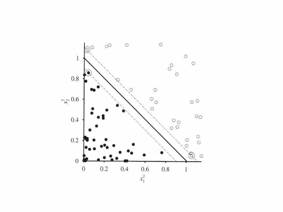
Learn linear rule in feature space. Example:

The separating hyperplane in feature space is

degree two polynomial in input space.

Transformation

• Instead of x1, x2 use

How do we find these features?

• F(x) =

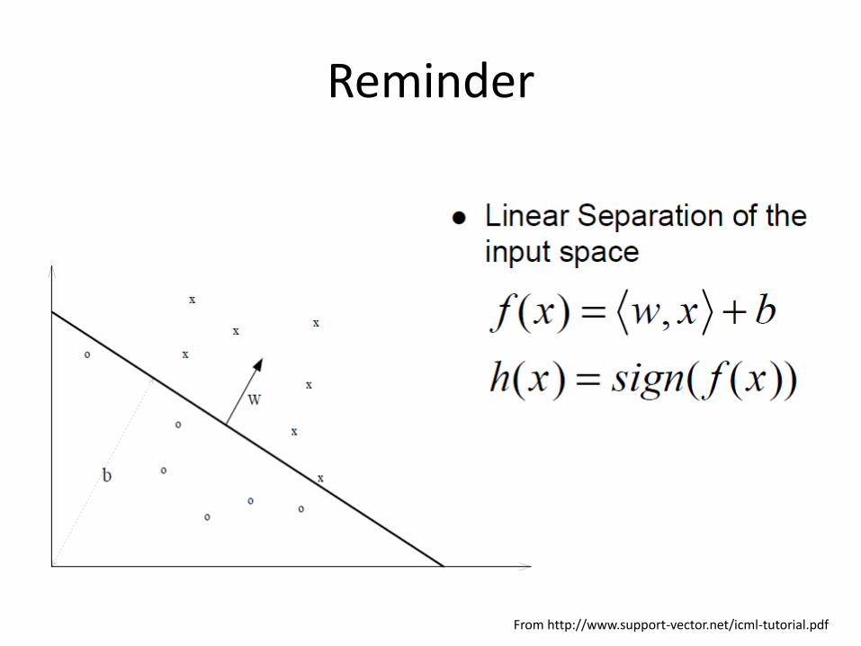
Reminder

From http://www.support-vector.net/icml-tutorial.pdf

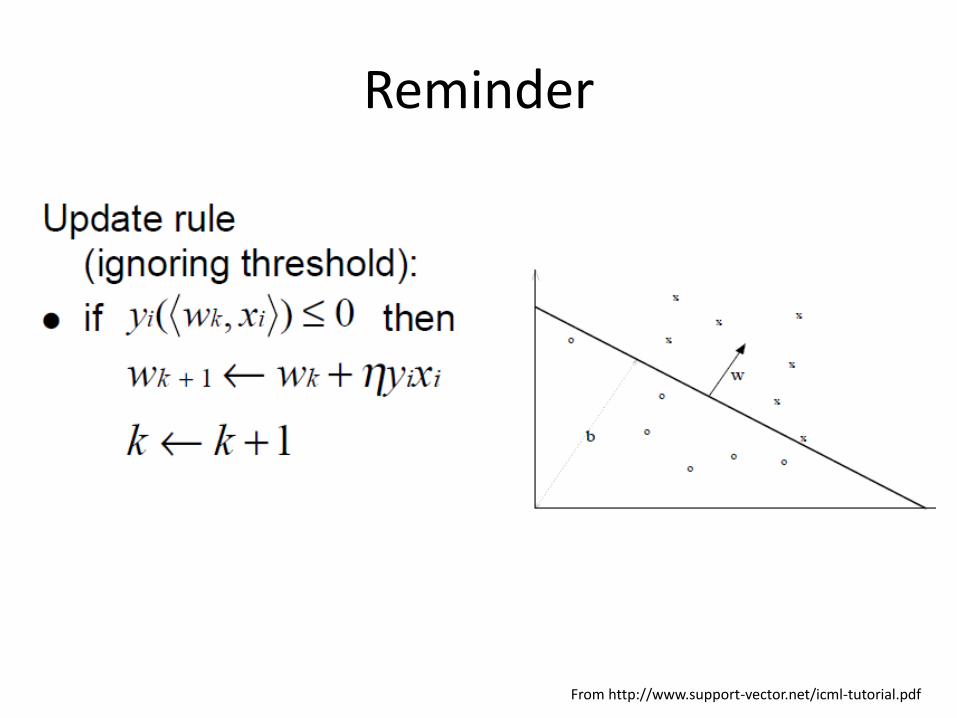
Reminder

From http://www.support-vector.net/icml-tutorial.pdf

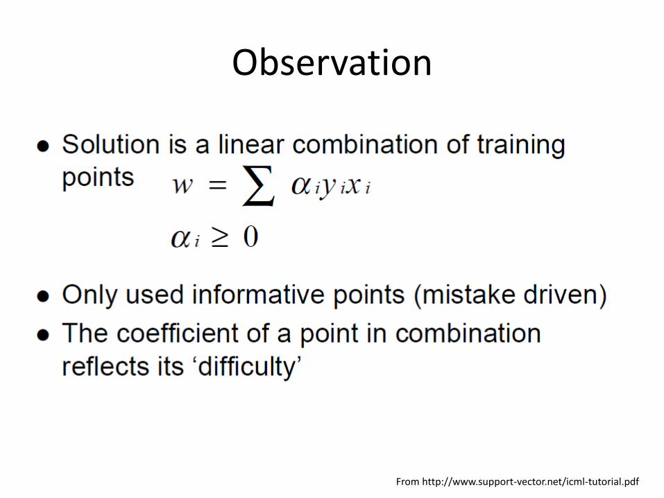
Observation

From http://www.support-vector.net/icml-tutorial.pdf

Dual Representation

From http://www.support-vector.net/icml-tutorial.pdf

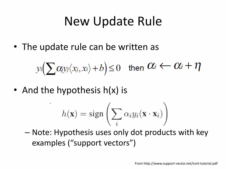
New Update Rule

• The update rule can be written as

• And the hypothesis h(x) is

– Note: Hypothesis uses only dot products with key examples (“support vectors”)

From http://www.support-vector.net/icml-tutorial.pdf

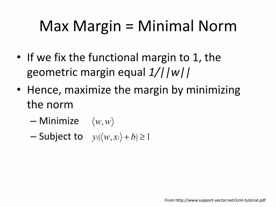
Max Margin = Minimal Norm

• If we fix the functional margin to 1, the geometric margin equal 1/||w||

• Hence, maximize the margin by minimizing the norm

– Minimize

– Subject to

From http://www.support-vector.net/icml-tutorial.pdf

How to find the ’s?

From http://www.support-vector.net/icml-tutorial.pdf

Using Kernels: Implicit features

• We need to compute <xi,xj> many times

– Or <F(xi),F(xj)> if we use features F(x)

• But what if we wound a set of features F(x) such that F(xi) F(xj) = (xixj)

2 ?

– Then we only need to compute (xixj)2

– We don’t even need to know what F is (!)

Implicit features: Example

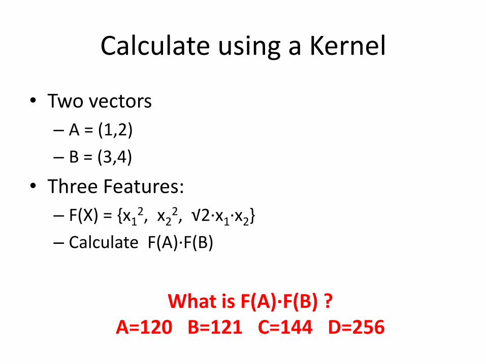
Calculate using a Kernel

• Two vectors

– A = (1,2)

– B = (3,4)

• Three Features:

– F(X) = {x12, x2

2, √2·x1·x2}

– Calculate F(A)·F(B)

What is F(A)·F(B) ? A=120 B=121 C=144 D=256

Calculate without using a Kernel

• A = (1,2), B = (3,4)

• F(X) = {x12, x2

2, √2·x1·x2}

– A=(1,2) F(A)={12, 22, √2·1·2} = {1, 4, 2√2}

– B=(3,4) F(B)={32, 42, √2·3·4} = {9, 16, 12√2}

• F(A)·F(B) = 1·9+4·16+2·12·2 = 121

Calculate using a Kernel

• A = (1,2), B = (3,4), F(X) = {x12, x2

2, √2·x1·x2}

• F(A)·F(B) = (A·B)2 = (1·3+2·4)2= 112 = 121

• We didn’t need to explicitly calculate or even know about the terms in F at all! – just that F(A)·F(B) = (A·B)2

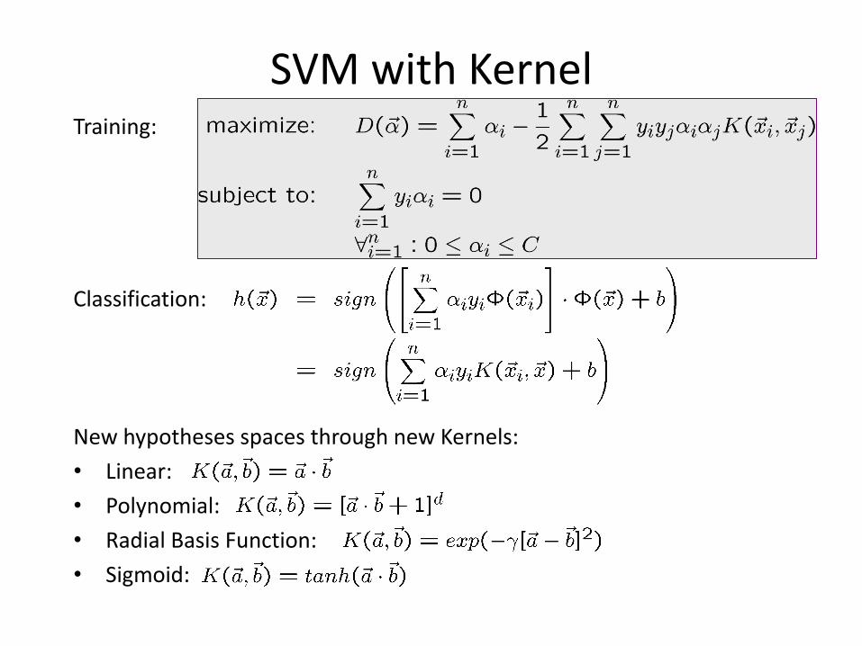
SVM with Kernel Training:

Classification:

New hypotheses spaces through new Kernels:

• Linear:

• Polynomial:

• Radial Basis Function:

• Sigmoid:

Solution with Gaussian Kernels

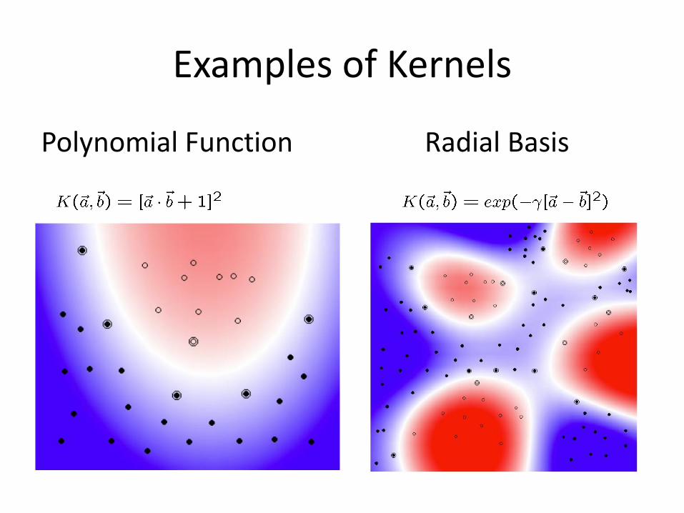
Examples of Kernels

Polynomial Function Radial Basis

Kernels for Non-Vectorial Data

Kernels for Non-Vectorial Data • Applications with Non-Vectorial Input Data classify non-vectorial objects – Protein classification (x is string of amino acids)

– Drug activity prediction (x is molecule structure)

– Information extraction (x is sentence of words)

– Etc.

• Applications with Non-Vectorial Output Data predict non-vectorial objects – Natural Language Parsing (y is parse tree)

– Noun-Phrase Co-reference Resolution (y is clustering)

– Search engines (y is ranking)

Kernels can compute inner products efficiently!

Properties of SVMs with Kernels

• Expressiveness – Can represent any boolean function (for appropriate

choice of kernel)

– Can represent any sufficiently “smooth” function to arbitrary accuracy (for appropriate choice of kernel)

• Computational – Objective function has no local optima (only one global)

– Independent of dimensionality of feature space

• Design decisions – Kernel type and parameters

– Value of C

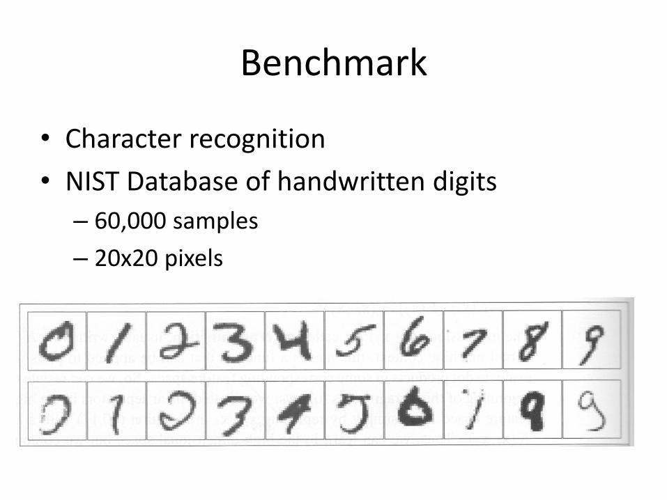
Benchmark

• Character recognition

• NIST Database of handwritten digits

– 60,000 samples

– 20x20 pixels

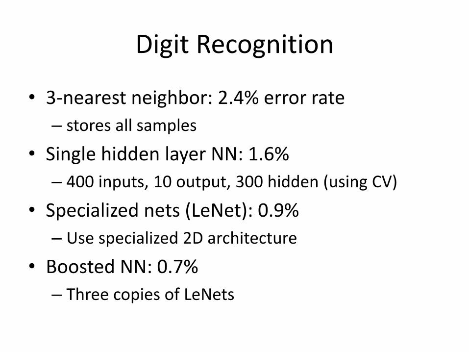
Digit Recognition

• 3-nearest neighbor: 2.4% error rate

– stores all samples

• Single hidden layer NN: 1.6%

– 400 inputs, 10 output, 300 hidden (using CV)

• Specialized nets (LeNet): 0.9%

– Use specialized 2D architecture

• Boosted NN: 0.7%

– Three copies of LeNets

Digit Recognition

• SVM: 1.1%

– Compare to specialized LeNet 0.9%

• Specialized SVM: 0.56%

• Shape Matching: 0.63%

– Machine vision techniques

• Humans?

– A=0.1% B=0.5% C=1% D=2.5% E=5%

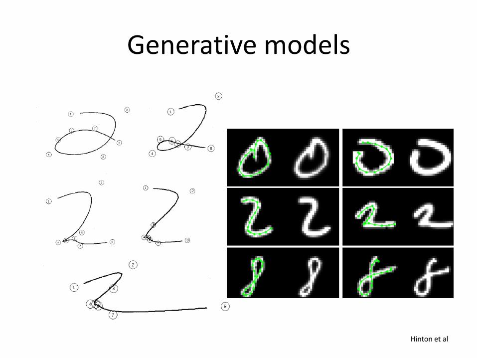
Generative models

Hinton et al

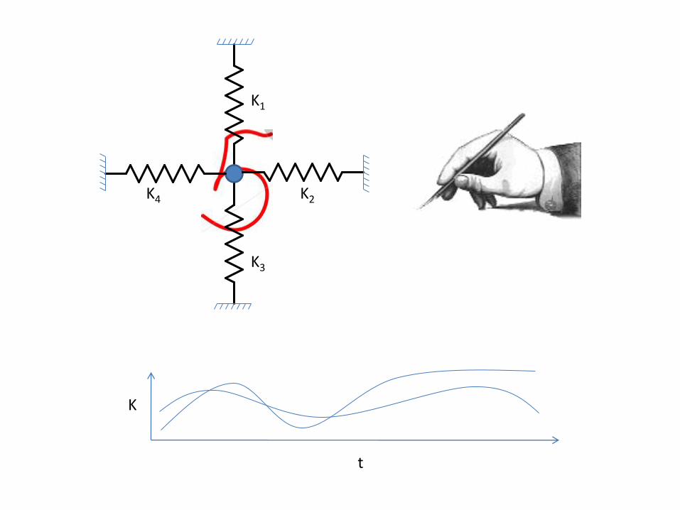
K1

K2

K3

K4

K

t